Post Syndicated from Explosm.net original https://explosm.net/comics/my-car
New Cyanide and Happiness Comic
Post Syndicated from Explosm.net original https://explosm.net/comics/my-car
New Cyanide and Happiness Comic
Post Syndicated from Werner Gunter original https://aws.amazon.com/blogs/big-data/amazon-redshift-multi-region-disaster-recovery/
Modern enterprises trust Amazon Redshift to power their most demanding analytics workloads and increasingly require multi-Region disaster recovery to protect those workloads against Regional disruptions. From real-time fraud detection and regulatory reporting to customer-facing dashboards processing millions of transactions daily, organizations are designing for resilience from day one. In financial services, for example, regulatory frameworks increasingly mandate geographic redundancy for data infrastructure, making cross-Region disaster recovery (DR) not only a technical consideration but a compliance requirement. A well-designed DR strategy keeps your analytics infrastructure available and responsive regardless of Regional disruptions, protecting revenue streams, maintaining regulatory standing, and preserving customer trust.
In our previous blog post, Implement disaster recovery with Amazon Redshift, we covered node-level recovery, Availability Zone (AZ) recovery, Multi-AZ deployments, cross-Region backup setup, CNAME implementation, Amazon Redshift Spectrum and Redshift Data sharing considerations.
In this post, we walk through the core concepts of cross-Region disaster recovery, introduce a framework for assessing your requirements, and then dive deep into three primary DR strategies for Amazon Redshift: Active-Passive, Active-Active, and a Hybrid approach. For each strategy, we cover architecture, trade-offs, implementation guidance, and cost considerations so you can make an informed decision for your workload.
Disaster recovery includes the set of policies, tools, and procedures that enable an organization to restore critical systems and data after an incident. It helps maintain business continuity during events such as a regional AWS outage, accidental data deletion, infrastructure failure, or a security event.
Any DR strategy depends on two key metrics:
These two numbers drive all architectural decisions for DR and understanding them helps clarify the trade-offs between various DR strategies.
Before selecting a strategy, you need to assess your workload’s criticality and your organization’s tolerance for data loss and downtime. Ask yourself:
The following table serves as a quick reference to match your requirements to a DR strategy:
| Requirement | Recommended strategy |
| RPO: 10–30 min, RTO: 1–2 hours, cost-sensitive | Active-Passive |
| RPO: Near-zero, RTO: Minutes, mission-critical | Active-Active |
| Mixed criticality across data tiers | Hybrid |
The following decision tree helps you select the right disaster recovery strategy based on your workload’s RPO and RTO requirements.
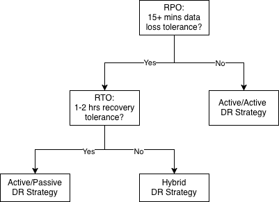
Regardless of which strategy you choose, the following practices apply universally to Amazon Redshift DR implementations.
Use multi-Region AWS KMS keys: Encrypt your Amazon Redshift clusters and S3 data with multi-Region AWS Key Management Service (AWS KMS) keys. This avoids the need to re-encrypt data during failover, which can add significant time to your RTO. Note that AWS KMS allows only one replica of a multi-Region key per AWS Region within the same partition. This is a service-level constraint. In most DR scenarios, a single multi-Region key per Region is sufficient since all resources in that Region can share the same key.
Automate with infrastructure as code: Define all DR Region infrastructure with infrastructure as code (IaC), such as Terraform, AWS CloudFormation, or AWS Cloud Development Kit (AWS CDK). IaC supports consistency between Regions, removes manual configuration errors, and enables rapid provisioning during failover. For organizations using Terraform Enterprise, verify that your workspace configuration supports multi-Region deployments.
Implement comprehensive monitoring. Use Amazon CloudWatch alarms where possible:
Early detection of replication failures is critical. A silent replication failure discovered during a disaster is far worse than one caught proactively. For detailed metrics monitoring configuration, see the Amazon CloudWatch alarms user guide.
Test quarterly. DR plans that aren’t tested regularly are more likely to fail during an actual disaster. Conduct quarterly failover tests that measure actual RTO and RPO against your targets. Validate data consistency post-failover. Document lessons learned and update your runbooks accordingly.
Use Amazon Redshift Spectrum. For cold and warm data tiers, you can query data directly in Amazon S3 without loading it into Amazon Redshift. This can reduce your data restoration requirements during failover. Remember that your cluster and S3 bucket must be in the same Region. Recreate external schemas in the DR Region pointing to your replicated S3 data. For Amazon Redshift Serverless endpoints and Redshift provisioned clusters without Spectrum, the DR strategy relies on snapshot replication and cross-Region restore. The same principles apply regardless of whether you use RA3 or RG (Graviton) node types.
In an active-passive configuration, your primary AWS Region runs the end-to-end workload, including data ingestion, processing, and serving data through Amazon Redshift. Amazon Redshift replicates data to the DR Region using its built-in cross-Region snapshot feature. During a disaster, you restore clusters from replicated snapshots in the DR Region.
RPO: 15 minutes plus time for data replication | RTO: 1–2 hours | Cost: Low
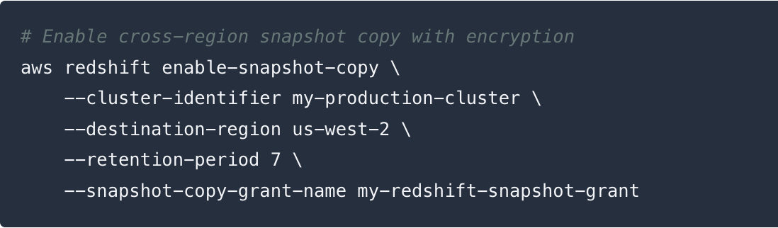
By default, Amazon Redshift provisioned clusters take a new snapshot every 8 hours, or whenever 5 GB of data changes are detected on any single node, whichever comes first. The 5 GB threshold is evaluated per node independently.
Amazon Redshift offers automated snapshots of your cluster at no extra storage cost in both your primary and DR Regions. You will incur charges for the data transfer when Amazon Redshift copies snapshots across Regions. The initial cross-Region copy is a full snapshot transfer. Subsequent copies are incremental, transferring only the changed blocks since the last snapshot, which significantly reduces transfer time and cost.
You can override the default and set a custom schedule, with a minimum frequency of once per hour. However, this is only useful in one scenario:
| Cluster type | Recommendation |
| ≥ 5 GB of changes per node per hour | Keep the default — already snapshotting frequently enough |
| < 5 GB of changes per node per hour | Customize the schedule to take snapshots more often |
If you need a guaranteed RPO of less than 1 hour (for example, every 15 minutes), or need to retain backups beyond 35 days, use manual snapshots scheduled at the frequency you want. Manual snapshots incur additional storage charges but are retained until explicitly deleted.
| Automatic snapshots | Manual snapshots | |
| Frequency | Every 8 hours or 5 GB change (customizable to run hourly) | Any frequency you choose |
| Best for | RPO ≥ 1 hour | RPO < 1 hour (for example, 15 min) |
| Cost | No additional cost (included with cluster) | Additional storage charges. |
| Retention | 1–35 days (configurable) | Until explicitly deleted |
| Cross-Region copy | Supported (incremental) | Supported (incremental) |
The following diagram illustrates the Active-Passive DR architecture.
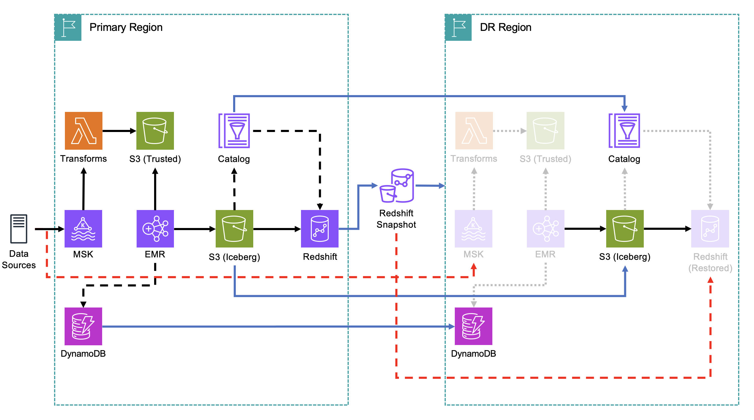
The Active-Passive strategy keeps compute resources in the DR Region ready to be spun up from snapshots when needed. When replicating data, consider the other services that are part of your end-to-end data pipeline. In the Amazon Redshift data sharing model, the producer cluster creates and owns the data, while consumer clusters read from the producer through data shares. In a DR context, the producer is restored first in the DR Region, then consumer clusters are resumed to serve read workloads.
DR Region (Passive) components:
Failover sequence (20–60 minutes):
In an Active-Active configuration, both your primary and DR Regions run fully operational data pipelines simultaneously. Data is ingested, processed, and served in both Regions at all times. Failover becomes a matter of redirecting traffic rather than restoring infrastructure. This reduces RTO to minutes.
RPO: Near-zero | RTO: < 1 hour (often minutes) | Cost: High
The following diagram illustrates the Active-Active DR architecture. Active-Active requires mirroring your entire pipeline, from ingestion through serving, across both Regions.
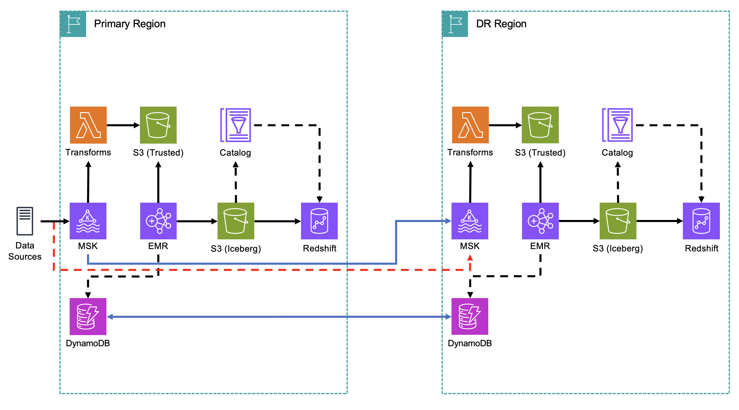
Real-time replication layer:
DR Region (Active) components:
Failover sequence (minutes):
Because the DR Region’s pipeline is already running, there is no infrastructure provisioning delay. Failover is primarily a configuration change.
Active-Active essentially doubles your infrastructure costs. You are running full Amazon MSK, Amazon EMR, and Amazon Redshift clusters in both Regions simultaneously. For large-scale deployments (1+ PB), this represents a significant ongoing investment. The business case rests on the cost of downtime exceeding the cost of duplicate infrastructure. This is a calculation that often favors Active-Active for customer-facing or regulatory workloads.
Not all data in your warehouse is equally critical. Some real-time insights and regulatory reports demand near-zero RPO, while historical trend analyses and archived compliance data can tolerate hours of recovery time. A Hybrid approach applies different DR strategies to different data tiers, optimizing cost while protecting what matters most.
RPO: Varies by tier | RTO: 30 minutes – 2 hours | Cost: Medium
The following diagram illustrates the Hybrid DR architecture.
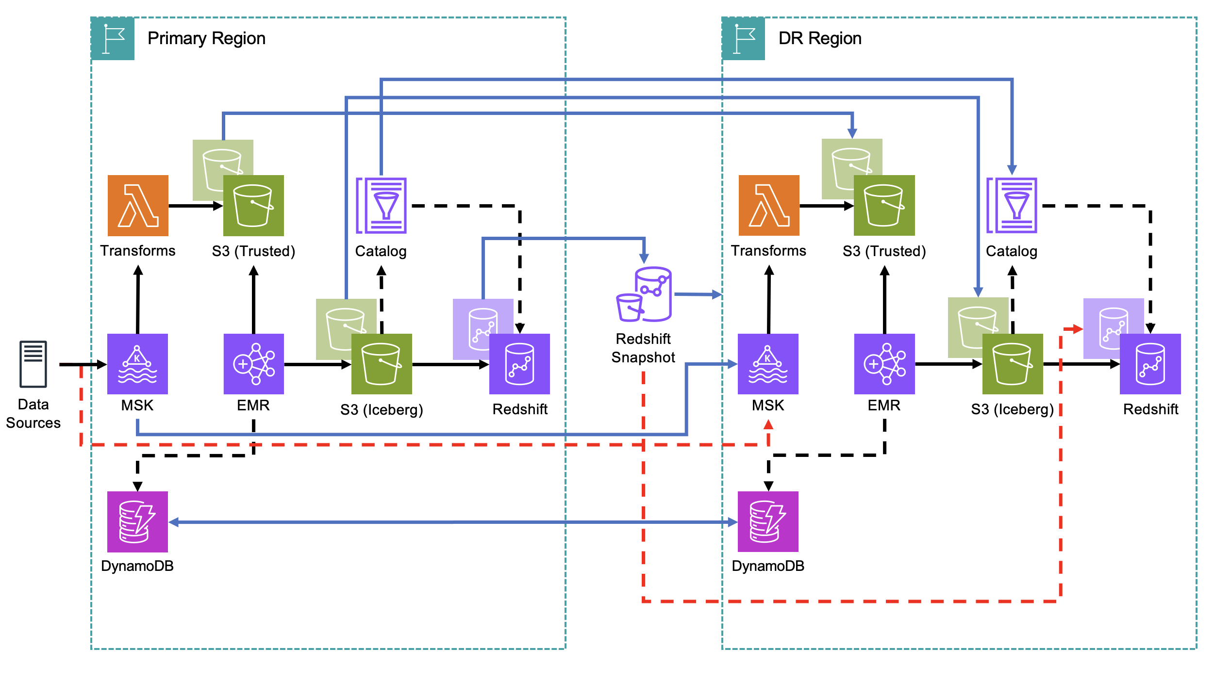
The Hybrid strategy requires a data model that supports clear separation at the schema or table level, with different recovery objectives applied per tier.
Tier 1: Hot data (Active-Active):
Tier 2: Warm data (Active-Passive):
Tier 3: Cold data (S3 replication only):
Schedule quarterly DR tests that include:
Disaster recovery for Amazon Redshift is not a one-size-fits-all problem. The right strategy depends on your RPO and RTO requirements, your data’s criticality, your ability to replay data from upstream sources, and your cost tolerance.
Whichever strategy you choose, the fundamentals remain the same: replicate early in the pipeline, automate your infrastructure, monitor replication health continuously, and test your failover procedures regularly. DR is not a project you complete. You maintain it as an ongoing practice.
Post Syndicated from Huyam Hasan original https://aws.amazon.com/blogs/big-data/streamline-apache-kafka-cluster-operations-and-migrations-with-agent-skills-for-amazon-msk/
Amazon Managed Streaming for Apache Kafka (Amazon MSK) manages core operational tasks for running Apache Kafka, including cluster provisioning, patching, high availability, and more. But operating Kafka clusters at scale still involves decisions that benefit from deep domain knowledge. For example, where do I start investigating application latency? How do I right-size a cluster to balance performance and cost? How do I analyze my applications, cluster configurations, and other requirements to support a smooth migration from self-managed Kafka to Amazon MSK?
With the new Agent Skills for Amazon MSK, you can access AI-assisted guidance for operations and migration planning directly in your development environment. Two complementary skills, managing-amazon-msk and migrate-to-msk, encode domain expertise based on AWS best practices, structured troubleshooting workflows, and programmatic sizing and compatibility analysis.
In this post, we walk through installing both skills and demonstrate their key capabilities. These include diagnosing a performance issue, sizing a cluster with cost breakdowns, and migration planning from self-managed Kafka to Amazon MSK including discovery, compatibility assessment, and target sizing.
Baseline large language models encode knowledge from their training data. That data can go stale as services evolve, and it often lacks the specific, contextual detail a task needs. As a result, a general-purpose assistant can produce answers that sound convincing but are factually wrong (hallucinations). For example, Amazon MSK Provisioned clusters come in two broker types, Standard and Express. Both broker types include their own considerations to achieve your performance, latency, availability, and durability requirements. Because training data mixes the two together, general-purpose assistants routinely conflate them and apply advice to the incorrect broker type.
These skills solve this problem by encoding the correct context for Amazon MSK broker operations, performance management, client configuration, and migrations, aligned with AWS best practices. This helps agents give more accurate, contextual guidance.
The two Amazon MSK Agent Skills cover the full lifecycle of Amazon MSK cluster ownership:
Operations expertise for Amazon MSK Provisioned clusters with both Standard and Express broker types:
| Workflow | What it does |
| Performance troubleshooting | Structured decision tree: CPU saturation, batch size analysis, Amazon Elastic Block Store (Amazon EBS) throughput entitlements (Standard), Express brokers entitlements |
| Consumer lag diagnosis | Determines if lag is broker-side, partition-level (hot keys), or client-side. Provides targeted fixes |
| Storage management | Amazon EBS expansion, auto scaling, retention planning, tiered storage (Standard only) |
| Cluster sizing and pricing | Programmatic right-sizing and cost estimate tool comparing all Standard and Express instance types with cost breakdowns |
| Monitoring and alarms | Set up actionable Amazon CloudWatch alarms with broker-type-aware thresholds that follow best practices for monitoring |
| Maintenance operations | Rolling restart impact analysis, patching and broker upgrades, version upgrade planning, and transient failure analysis (distinguishing expected maintenance disruptions from real issues). |
Migration planning from self-managed Apache Kafka to Amazon MSK in three phases:
| Phase | What it does |
| Discovery | Inventories your source cluster from infrastructure as code (IaC) files, Kafka CLI output, or manual input. Produces a standardized cluster-config.json |
| Assessment | Five-pillar compatibility check (topology, version, configs, auth, quotas) plus target cluster sizing using the AWS-published Amazon MSK Sizing and Pricing workbook |
| Simulation (Optional) | Deploys temporary Amazon MSK cluster and Amazon EC2 load-generation fleet in your account to test performance under synthetic load before you migrate. Produces an Amazon CloudWatch dashboard with throughput, broker health, latency, and consumer lag metrics. |
After assessment, the skill provides guidance on using Amazon MSK Replicator for the actual data migration to your new Amazon MSK cluster.
To use the tool, you need:
Both skills are available in the Agent Toolkit for AWS on the GitHub website.
After initial setup following the steps in the Agent Toolkit instructions, install the Amazon MSK skills with:
For more information on managing skills, refer to Managing skills with the AWS CLI in the Agent Toolkit for AWS User Guide.
Verify MCP installation by checking the MCP server status in your IDE’s MCP panel.
Verify skill installation with:
You should see both skills listed for your detected agents. To confirm they’re active, ask your AI assistant an Amazon MSK question, and it should load the skill to engage with broker-type-aware guidance.
During your evaluation of Amazon MSK your team notices elevated produce latency. You ask the AI assistant for help,
“Our Amazon MSK Express broker cluster is experiencing high produce latency that we think is related to our client application. The producer code is in this working directory. Can you help diagnose?”
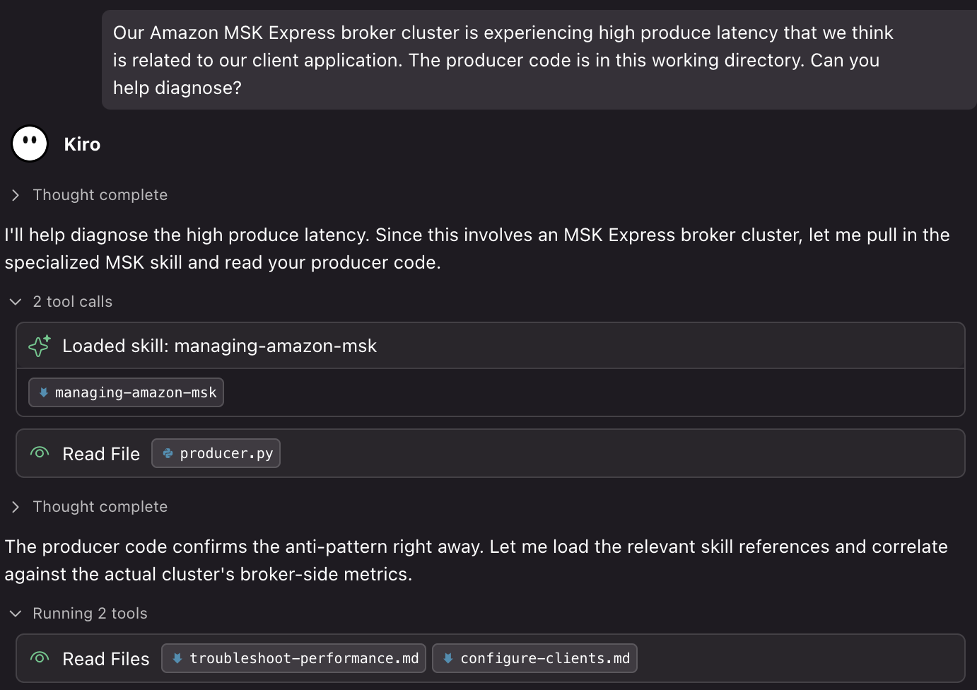
The agent immediately identifies that this question would be well suited for the managing-amazon-msk-skill and activates it. In the same step, the agent opens your producer code to diagnose the real client configuration. The skill ships with reference guides, and the agent selects the two that matter for this specific problem. It then maps your application code directly onto the skill’s diagnostic workflow, landing on a diagnosis:
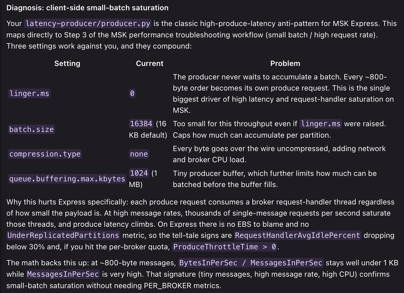
The skill identifies three compounding anti-patterns in the configuration, specifically linger.ms=0, an undersized batch.size, and compression.type=none. It then explains why they negatively impact Kafka cluster performance: every tiny message becomes its own produce request, saturating broker request-handler threads. Based on these observations, the skill delivers a targeted solution:
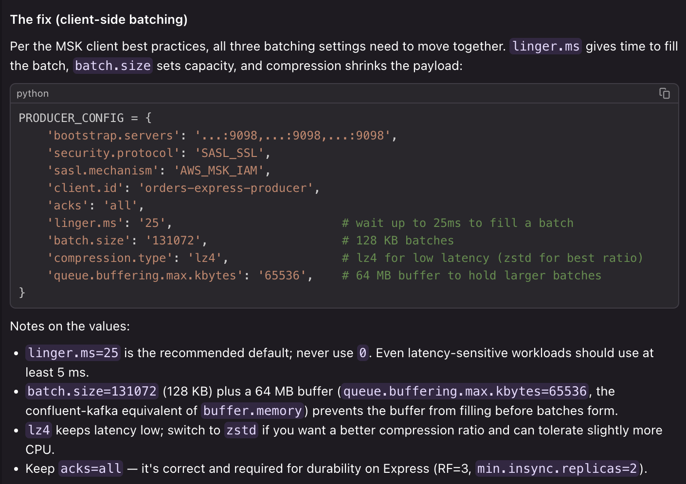
The skill uses best practice client-configuration references to provide specific recommendations to improve your application. It then goes on to provide additional context, considerations, and the Amazon CloudWatch metrics to observe to verify that the configurations have improved your end-to-end performance.
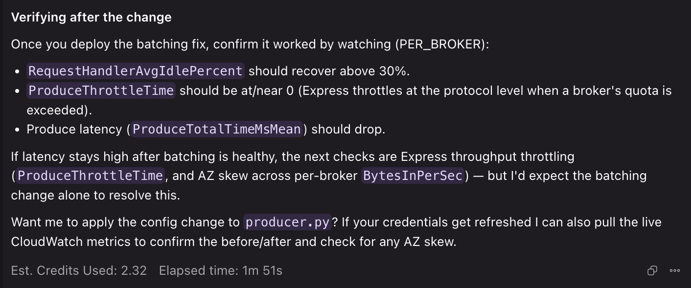
You can try this yourself by bringing your own producer code and letting the skill diagnose it. If you give it access to the AWS CLI the agent can pull live Amazon CloudWatch metrics from your actual cluster. This lets it correlate broker-side signals with what it sees in your client configuration for a more complete diagnosis.
The migrate-to-msk skill guides you through a structured migration from self-managed Apache Kafka to Amazon MSK in three phases: discovery, assessment, and optional simulation. When you prompt the skill, it launches the discovery phase.
In this scenario, you point the skill at your infrastructure as code (IaC) files describing a self-managed Kafka deployment:
“Here’s our Kafka infrastructure, can you help us plan a migration to Amazon MSK Express brokers?”
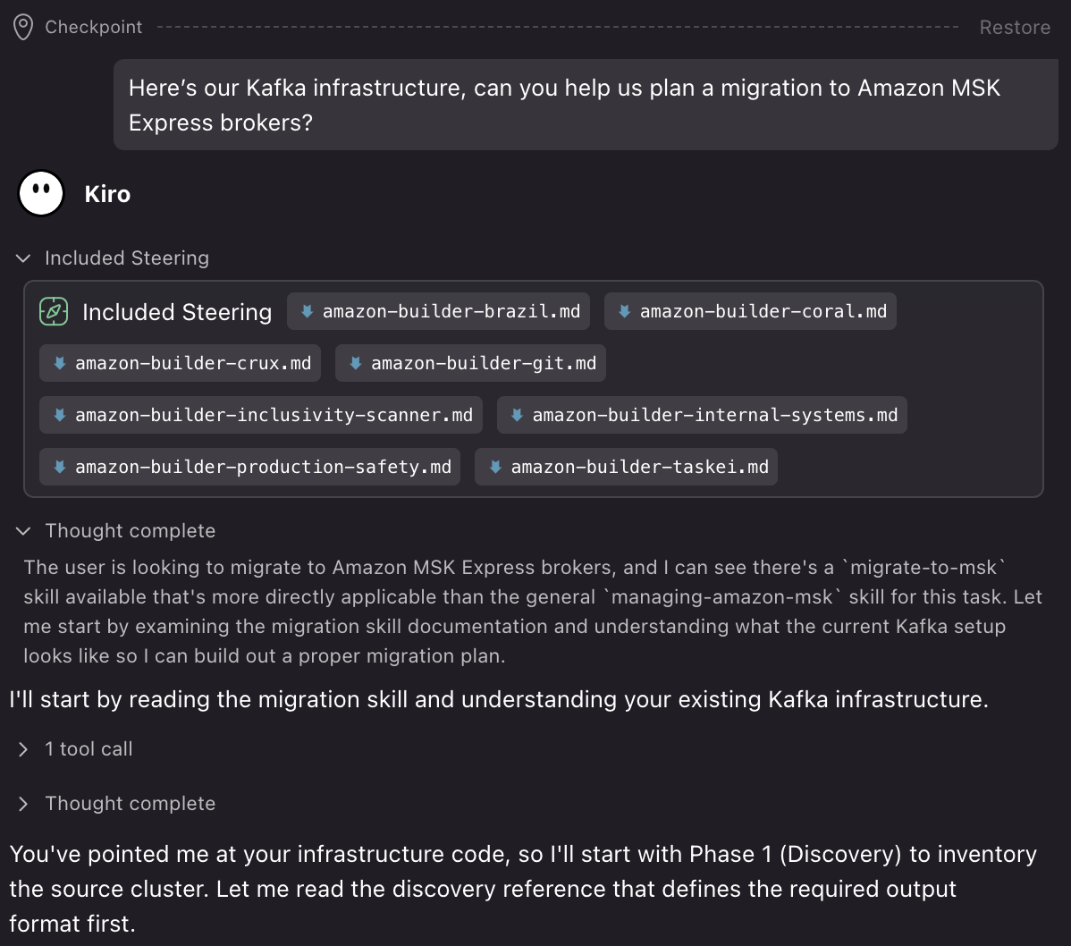
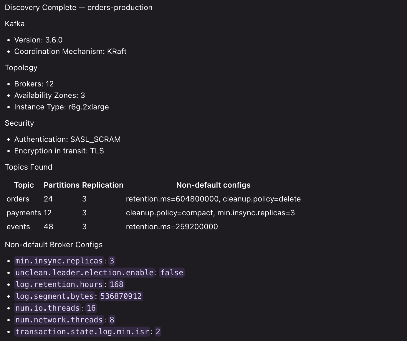
The skill pulls static details: broker topology, versions, security configuration, and topic definitions directly from your IaC files.
For runtime values the skill can’t derive from IaC, such as actual peak throughput or consumer-group count, the skill identifies these as flagged gaps. For each gap, the skill provides the specific Kafka CLI commands you can run against your live cluster to capture those values.
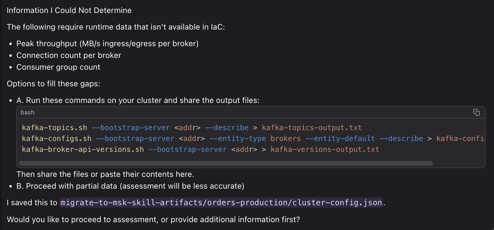
The skill supports discovery from multiple source types: Terraform, CDK, CloudFormation, Docker Compose, Kubernetes manifests, or manual input in conversation.
With discovery complete, the assessment phase runs two independent analyses against your current cluster infrastructure.
Compatibility assessment evaluates your source cluster across five pillars:
| Pillar | What it checks |
| Topology | AZ count, broker count, KRaft or ZooKeeper |
| Kafka version | Source version against Amazon MSK supported set (3.6, 3.8, 3.9) |
| Configs | Broker and topic configs against Amazon MSK’s editable/enforced/range-restricted sets |
| Auth | Authentication mechanism compatibility |
| Quotas | Peak workload against Amazon MSK per-broker ceilings |
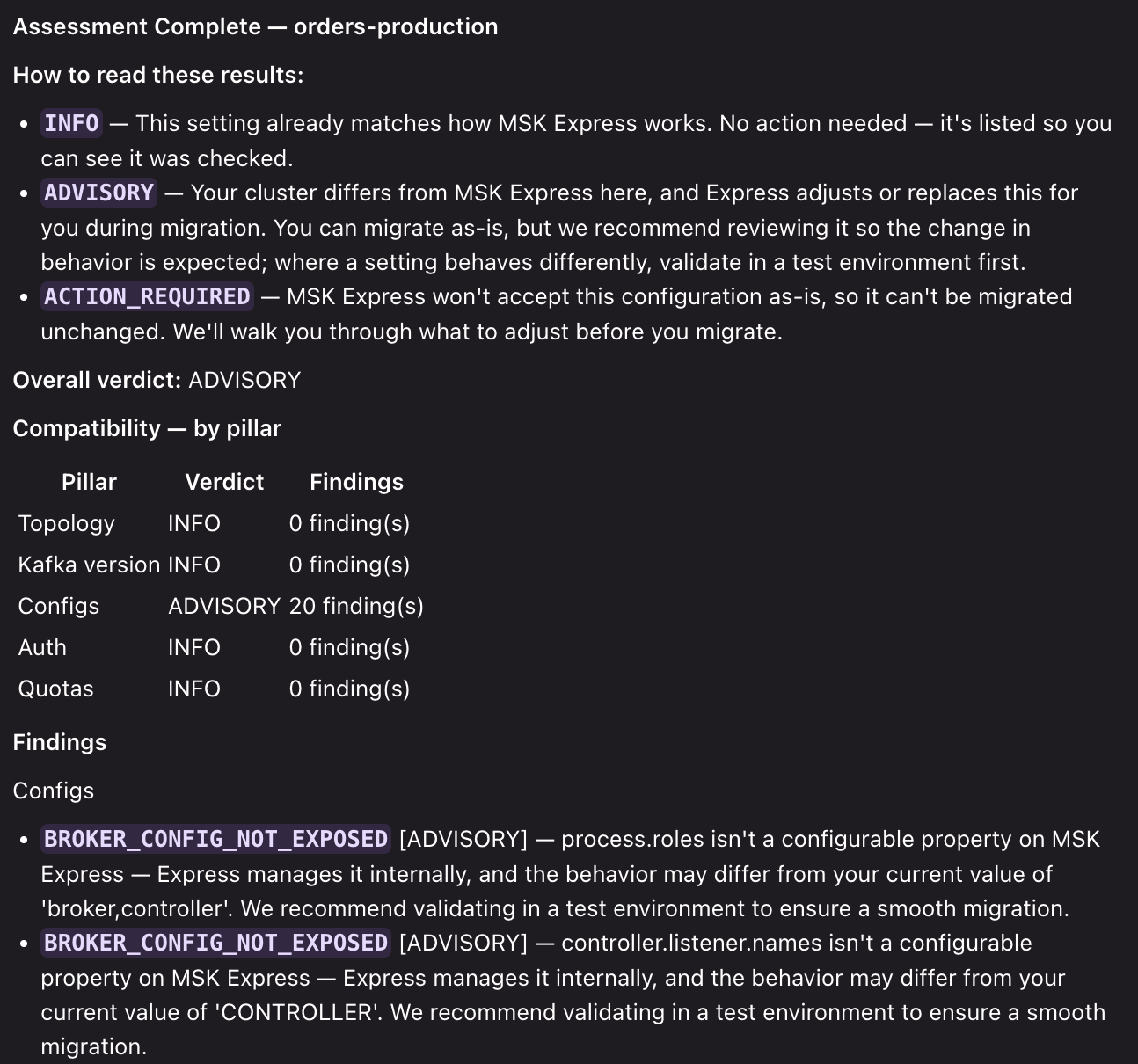
Each pillar produces one of the following finding types:
| Verdict | Meaning |
INFO |
Already aligns with Amazon MSK. No action needed. |
ADVISORY |
Amazon MSK handles this differently, but migration can proceed. Review so the behavior change is expected. |
ACTION_REQUIRED |
Amazon MSK will not accept this in its current form. Remediation recommended. |
Target sizing uses your current cluster’s usage metrics to perform right-sizing for Amazon MSK, including instance type, broker count, and projected monthly cost for your workload. This gives you a shareable artifact to use for sizing against different inputs and assumptions.
Next, you ask the skill to run the assessment:
“Assess my cluster for Amazon MSK Express broker compatibility and size the target”:
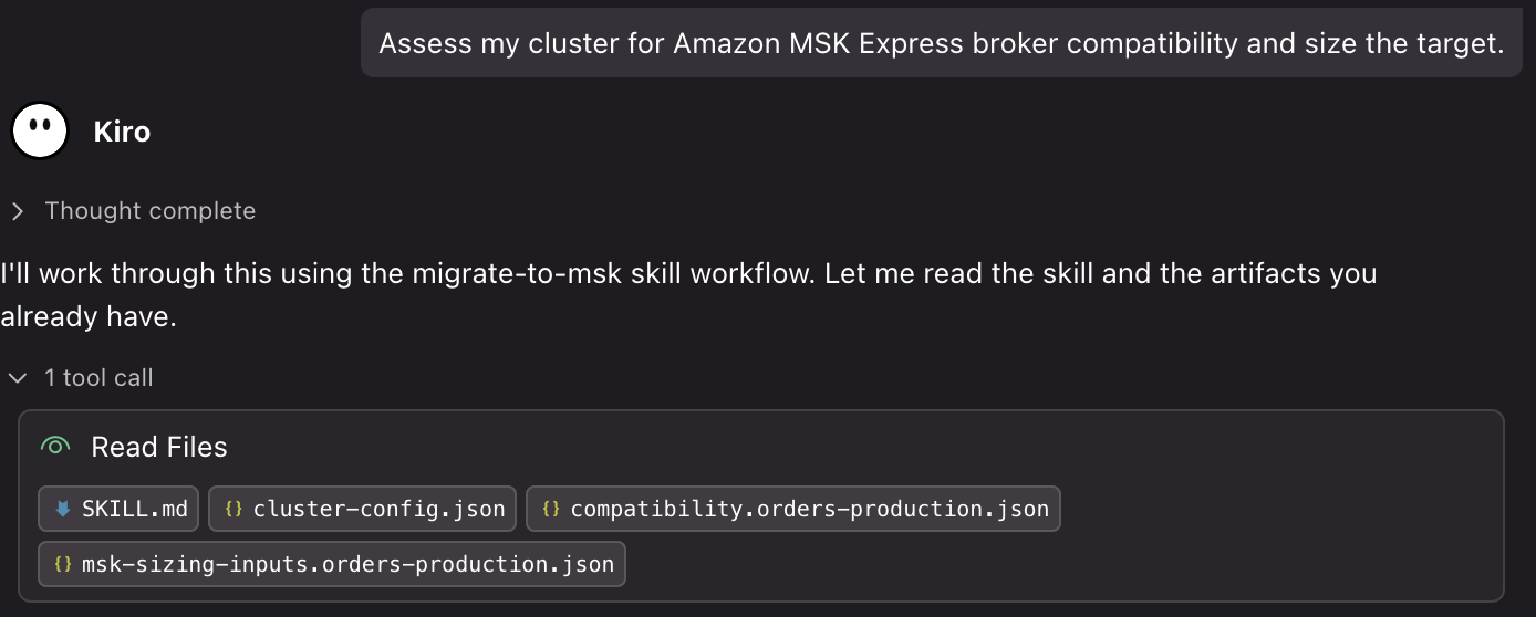
The skill runs both analyses against your cluster configuration. It outputs a compatibility report, sizing inputs, and sizing outputs, giving you a complete picture of what needs attention before migration and what your target cluster should look like.
Once you’ve validated compatibility and provisioned your Amazon MSK Express brokers, Amazon MSK Replicator handles the actual data migration. Amazon MSK Replicator is the native AWS solution for replicating data between Amazon MSK Provisioned clusters. For migrations, it supports replication of data from self-managed Apache Kafka clusters (including on-premises, self-hosted on AWS, or other cloud providers) to Amazon MSK Provisioned clusters.
With assessment complete, you can optionally ask the skill to guide you through setting up a live test environment:
“Can we run a simulation to see how Amazon MSK Express brokers handle our workload before we commit to migrating?”
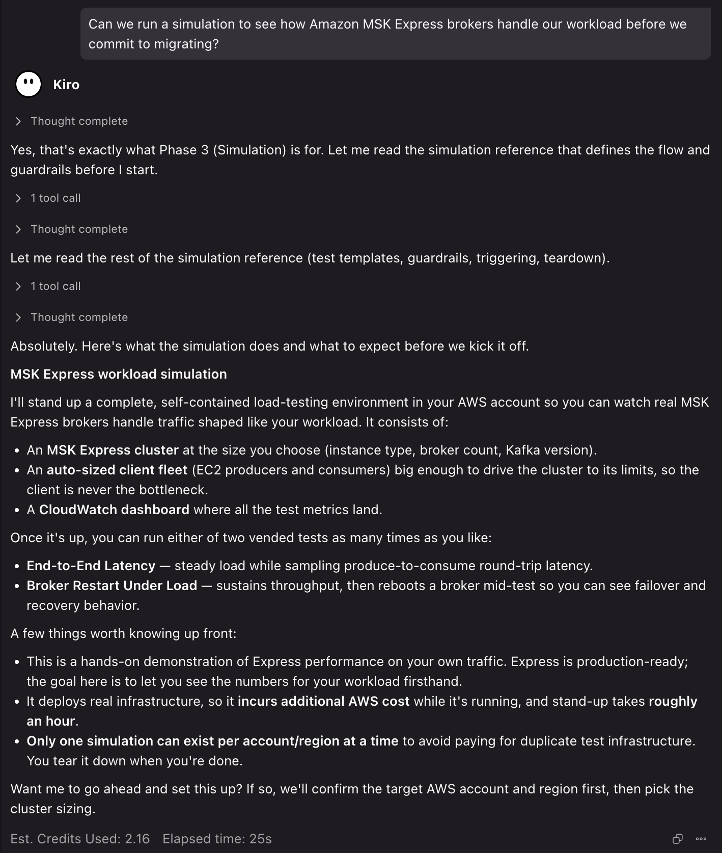
The skill walks you through deploying temporary Amazon MSK Express brokers and EC2 client fleet in your own AWS account. These are sized from your Phase 2 workbook or numbers you provide, so that you can see real performance on your actual workload rather than relying on estimates. It confirms the target account and permission before deploying any billable resources.
Once the cluster is up, you choose a provided test (end-to-end latency or broker restart under load), and the skill runs it. It then surfaces metrics related to throughput, broker health, latency, and consumer lag on a CloudWatch dashboard. When you’re done, the skill helps you tear the stack down so you stop incurring cost.
You’re planning a new streaming workload and need to determine the right configuration:
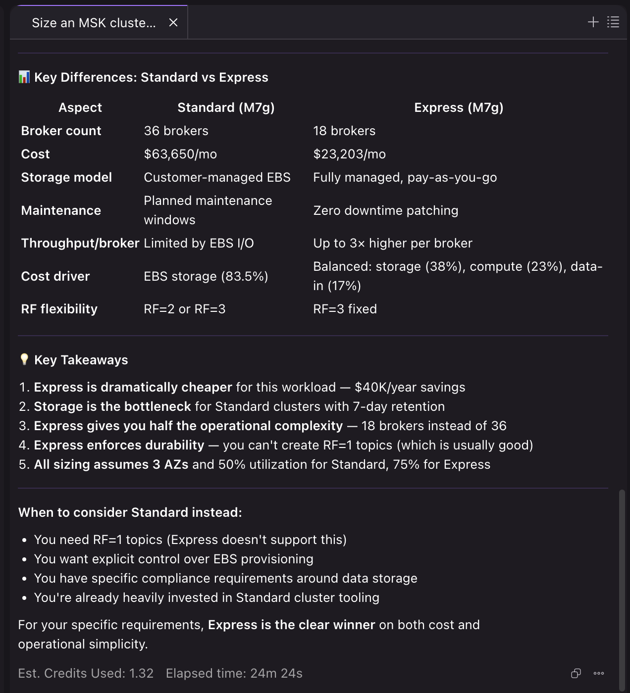
“Size an Amazon MSK cluster for 200 MiB/s peak ingress, 600 MiB/s peak egress (3 consumer groups), 1,500 partition replicas, 168 hours retention. Compare Standard and Express.”
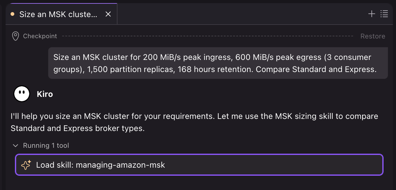
The skill’s programmatic sizing calculator evaluates your workload against every available instance type simultaneously, sizing across four constraints: ingress capacity, egress capacity, partition limits, and storage volume. Each is rounded up to a multiple of 3 Availability Zones (AZs).
When you ask the skill to size a cluster, it uses its sizing script to identify and recommend the least expensive viable option per broker class, and to break down the cluster cost across various sizing dimensions.
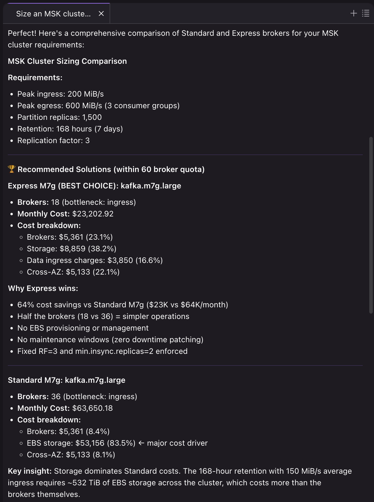
The calculator accounts for factors that manual sizing often misses, such as replication overhead on EBS, network bandwidth, and cross-AZ data transfer costs. The skill flags exactly which constraint is the bottleneck for each instance type, so you understand why a particular broker count was chosen.
Both skills recommend Transport Layer Security (TLS) encryption and IAM authentication. Discovery and assessment outputs contain broker addresses and configuration details. Treat them as sensitive and avoid sharing them in public channels without redaction. The migration artifacts do not store passwords or secrets.
If you ran the optional Simulation phase with the migrate-to-msk skill, it deployed real resources in your AWS account, including an Amazon MSK Express cluster and an EC2 load-generation fleet, that continue to incur charges until you delete them. Ask the skill to tear down the simulation, or delete its CloudFormation stack yourself, to stop incurring cost. Only one simulation can exist per account at a time.
Migration artifacts (migrate-to-msk-skill-artifacts/) are local files that you can delete at your discretion.
Traditionally, Kafka administrators have relied on web-based UIs and dashboards for cluster health management and troubleshooting. With these skills, you can accelerate agent workflows that integrate directly into development environments and DevOps processes. Amazon MSK aims to expand this Agent Skills portfolio with additional tools and capabilities, so customers can build more sophisticated agentic DevOps workflows for their streaming infrastructure.
The Amazon MSK Agent Skills bring structured, broker-type-aware expertise to operating and migrating Amazon MSK clusters. Instead of searching through documentation to determine whether a metric applies to Standard or Express, or manually cross-referencing compatibility matrices for a migration, you get targeted guidance that routes to the correct path based on your cluster’s actual configuration.
Get started by installing both skills from the Agent Toolkit for AWS on the GitHub website into your development environment. Then try a prompt like:
“Size Amazon MSK Express brokers for 100 MiB/s ingress with 3 consumer groups and 72-hour retention”
or
“My Amazon MSK Express brokers have high produce latency. Help me diagnose”
The skills support you at any stage in the cluster lifecycle.
To learn more, visit the Amazon MSK documentation or open the Amazon MSK console. Have questions or feedback? Open an issue in the Agent Toolkit for AWS repository on the GitHub website.
Post Syndicated from Micah Walter original https://aws.amazon.com/blogs/aws/aws-weekly-roundup-price-reduction-of-gpt-models-in-bedrock-cloudwatch-managed-collectors-for-prometheus-metrics-and-more-august-3-2026/
 Last week I had the joy of participating in Amazon’s “Bring Your Kids to Work Day” with my 7 year old son. We commuted together into the New York City office, his first real rush hour train ride, and spent the day exploring how Amazon uses AI, machine learning, and robotics to deliver packages to customers all over the world. Watching his eyes light up as he saw robots navigating a fulfillment center reminded me why so many of us got into technology in the first place. There’s nothing quite like seeing that sense of wonder when something complex clicks.
That same energy carried into the week’s launches. We’ve got updates across AI pricing, observability, multicloud networking, and data management. Let’s dive in.
Headlines
Amazon Bedrock announces up to 80% lower prices for OpenAI GPT‑5.6 models – If you’re using OpenAI’s GPT‑5.6 family through Amazon Bedrock, your costs just dropped significantly. Effective July 30, on-demand inference prices for GPT‑5.6 Luna are reduced by 80%, while GPT‑5.6 Terra prices are reduced by 20%. Luna now costs $0.20 per million input tokens and $1.20 per million output tokens, making it one of the most affordable frontier-class models available. These price reductions apply automatically — no action required on your part. Read more
Last week’s launches
Here are some launches and updates from this past week that caught my attention:
Other AWS news
Here are some additional posts and resources that you might find interesting:
Upcoming AWS events
Check your calendar and sign up for upcoming AWS events:
Join the AWS Builder Center to connect with builders, share solutions, and access content that supports your development. Browse here for upcoming AWS-led in-person and virtual events and developer-focused events.
That’s all for this week. Check back next Monday for another Weekly Roundup!
Post Syndicated from Vara Bonthu original https://aws.amazon.com/blogs/big-data/introducing-apache-spark-troubleshooting-agent-for-amazon-emr-on-eks/
Debugging a failed Apache Spark application on Amazon EMR on EKS often means correlating signals from several places at once. These signals include Spark driver and executor pod logs, Spark event logs, and container termination signals that surface as pod exit codes rather than clear Spark errors. For example, a single out-of-memory failure can appear as a Kubernetes exit code 137 with no obvious link back to the line of code or configuration that caused it. This cross-system investigation can extend a single incident’s mean-time-to-resolution (MTTR) to days and requires deep Spark and Kubernetes expertise.
We recently announced Amazon EMR on EKS now supports Apache Spark troubleshooting agent extending the Apache Spark troubleshooting agent to support Amazon EMR on EKS. The agent already helps data engineers diagnose Spark failures on Amazon EMR on EC2, Amazon EMR Serverless, and AWS Glue using natural language prompts. With this launch, you can now point the same workflow at a failed Amazon EMR on EKS job run. From a single natural language prompt, the agent automatically retrieves your Spark logs from Amazon Simple Storage Service (Amazon S3) or Amazon CloudWatch (depending on your job’s logging configuration) along with Spark History Server Event log data, identifies the root cause, and recommends a fix when the failure is code-related. This can help reduce incident MTTR from days to minutes. Amazon EMR on EKS customers can use the agent at no additional cost. You only pay for your existing Amazon EMR on EKS resources.
In this post, we show you how to set up the agent for Amazon EMR on EKS and walk through troubleshooting a failed job run. We demonstrate the workflow from both the Amazon EMR console and an AI assistant that supports the Model Context Protocol (MCP), an open standard for connecting AI assistants to external tools and data.
The troubleshooting agent exposes a single interface to diagnose failed Spark applications across Amazon EMR on EKS, Amazon EMR on EC2, Amazon EMR Serverless, AWS Glue, and Amazon SageMaker notebooks. Instead of navigating different consoles, APIs, and log locations for each service, you describe your failed job in natural language, and the agent handles the rest. You can reach the agent from the Amazon EMR console or from MCP-compatible AI assistants, such as Kiro CLI, Kiro IDE, or Claude Code. We walk through both later in this post.
The troubleshooting agent runs as a fully managed MCP server, so you do not need to deploy or maintain a local MCP server. It uses a single-tenant design to keep your application data and code isolated. Operations are read-only and governed by AWS Identity and Access Management (IAM) permissions. The agent can only access the resources and actions your IAM role grants. Tool calls are automatically logged to AWS CloudTrail for complete auditability.
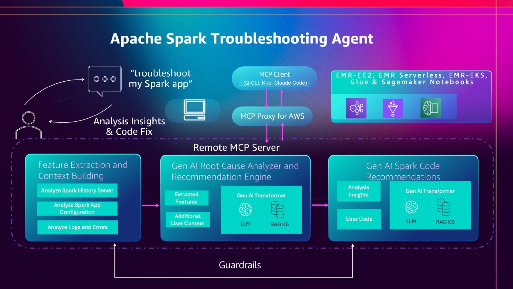
What’s specific to Amazon EMR on EKS is how the agent gathers its inputs. On Amazon EMR on EKS, your Spark driver and executor logs can be delivered to Amazon S3, Amazon CloudWatch Logs, or both, depending on your job’s monitoring configuration. The agent handles both sources automatically:
stderr/stdout logs from your S3 log location, including discovering executor pod logs.Drawing on years of AWS experience running millions of Spark applications at scale, the agent extracts the relevant features and signals from these sources, work that would otherwise require manual correlation across Amazon S3, Amazon CloudWatch, and the Spark UI. It then uses a large language model on Amazon Bedrock, grounded in a managed knowledge base of Spark and AWS troubleshooting expertise through Retrieval Augmented Generation (RAG), to produce a root cause analysis and, when the failure is code-related, a code recommendation.
The large language model (LLM), the knowledge base, and the retrieval that connects them are fully managed as part of the agent. There’s nothing for you to provision, host, or tune. This managed inference is provided at no additional cost for Amazon EMR on EKS. You pay only for the AWS resources you already use to run your Spark applications and to validate recommended changes.
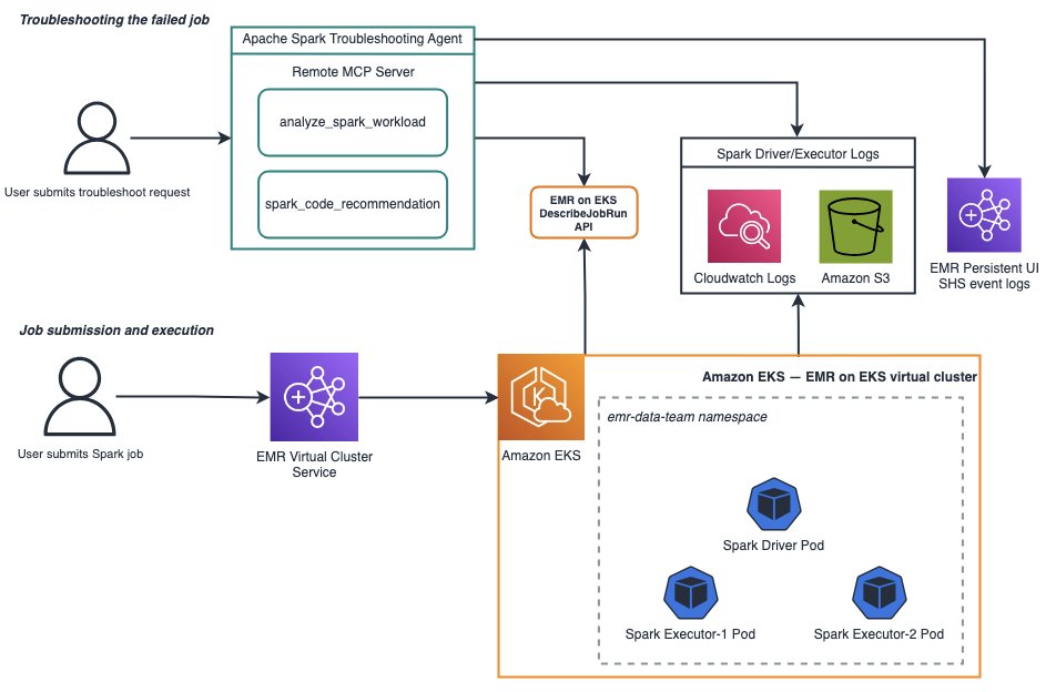
You can use the agent from either the Amazon EMR console or an MCP client. Both rely on setting up a single IAM role. The following sections walk through creating that role and then troubleshooting a failed job run with each method.
The IAM role grants the agent read access to the diagnostic sources it analyzes, such as your Amazon EMR on EKS job runs, the Amazon EMR Persistent UI, and your Spark logs in Amazon S3 and Amazon CloudWatch. Creating this role is the only setup required for the console experience. The MCP client path has a few additional prerequisites, covered later in the section on troubleshooting from an MCP client.
To run the commands in this section, you need the AWS Command Line Interface (AWS CLI) (version 2.30.0 or later) installed and configured with your AWS credentials. For instructions, see Setting up the AWS CLI.
The agent uses your IAM role to authorize operations at the AWS service level. It can only access what your role allows. Create a role your account can assume, then attach a policy granting the permissions the agent needs for Amazon EMR on EKS.
First, set some variables for the commands that follow. ACCOUNT_ID is derived from your configured credentials. Set REGION to the AWS Region where you run your Amazon EMR on EKS workloads:
Create a trust policy that allows your account to assume the role, and create the role:
Create and attach a policy granting the agent read access to your Amazon EMR on EKS job runs, the Amazon EMR Persistent UI, and your S3 and CloudWatch logs. Replace amzn-s3-demo-logging-bucket with the name of your logging bucket and replace my_log_group_name and my_log_stream_prefix with your CloudWatch log group name and log stream prefix, respectively.
Note: If you prefer an automated setup, an AWS CloudFormation template that creates this role with the required permissions is available in the setup documentation. The previous CLI steps give you the same result with finer control over each permission.
You can reach the troubleshooting agent two ways: directly from the Amazon EMR console, or from an MCP-compatible AI assistant such as Claude Code. We walk through both, using two different failures to show the range of what the agent diagnoses.
The console offers the fastest path. Once you’ve created the IAM role in the Set up IAM permissions section, no additional setup is required. Here we troubleshoot a job that failed with a driver out-of-memory error. The application generates a large dataset and calls collect() to pull it back to the driver, exceeding the configured spark.driver.maxResultSize of 512 MiB.
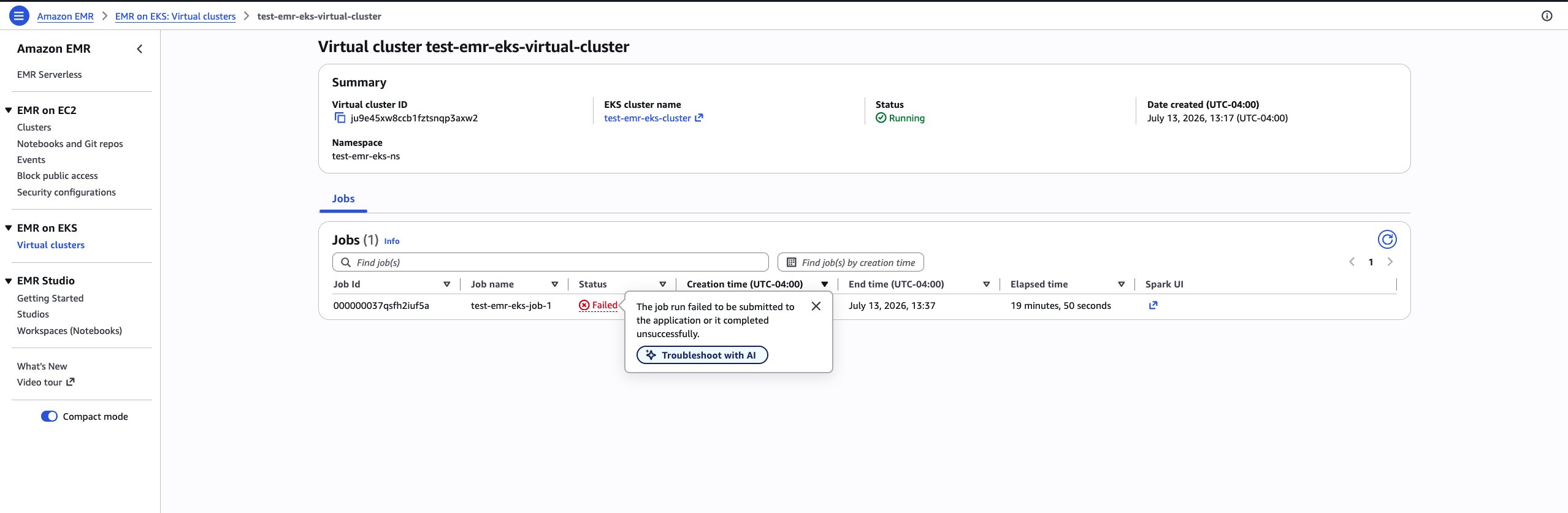
collect() operation on line 24 attempts to materialize the full result set on the driver, exceeding the spark.driver.maxResultSize safety limit. This fails the job before an actual driver out-of-memory crash. Because the failure stems from the application code, the agent also returns a code recommendation: a before-and-after diff that replaces the collect() call with a distributed write to the destination path. Executors then persist their partitions in parallel instead of funneling the data through the driver.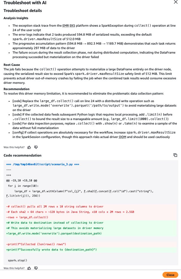
You can also use the agent from MCP-compatible AI assistants. This option requires a one-time setup to connect the assistant to the agent’s MCP servers, and it unlocks a conversational workflow where the agent chains from analysis into a concrete code fix. In this walkthrough, we use Claude Code.
In addition to the IAM role from the Set up IAM permissions section, the MCP client path requires:
uv package manager. For instructions, see Installing uv.Configure a profile that assumes the IAM role you created, so the MCP servers call AWS with the agent’s permissions:
The troubleshooting agent provides two tools through two MCP servers: analyze_spark_workload (workload analysis and root cause) and spark_code_recommendation (code fixes). Add both to your assistant.
For Claude Code:
Verify your setup by running the /mcp command in Claude Code to confirm the sagemaker-unified-studio-mcp-troubleshooting and sagemaker-unified-studio-mcp-code-rec servers are connected and their tools are available.
For Kiro CLI:
Verify with the /tools command in Kiro CLI to confirm the analyze_spark_workload and spark_code_recommendation tools are available.
For this walkthrough, we troubleshoot a different failure to show how the agent chains from analysis into a concrete code fix. The job is a small PySpark application that reads a CSV file into a DataFrame and registers it as a temporary view named people. It runs a Spark SQL query to uppercase the Name column before displaying the results. The job run failed because the query calls UPPERX, a function that doesn’t exist in Spark SQL (it’s a typo for the built-in UPPER).
From the Claude Code terminal (or MCP-compatible assistants), describe your failed job run in natural language, providing the virtual cluster ID and job run ID:
The agent invokes the analyze_spark_workload tool, which automatically:
For this job, the agent returns:
Root cause: SQL function error. Your Spark SQL query references a function UPPERX that doesn’t exist in an available function catalog (system.builtin, system.session, or spark_catalog.default). Category: SQL_ERROR. The job failed because the function name can’t be resolved. UPPERX is almost certainly a typo for the built-in UPPER function.
Because the failure is code-related, the agent then chains into the spark_code_recommendation tool, which produces a concrete before-and-after fix:
The two tools work together. analyze_spark_workload identifies the root cause, and when the failure stems from the application code, spark_code_recommendation returns the exact edit to make. You review the recommendation and apply it with full control over the change. The agent only provides the analysis and recommendations.
The troubleshooting agent diagnoses a wide range of Apache Spark failures on Amazon EMR on EKS, including:
collect() and executor terminations that surface as Kubernetes pod exit codes (such as exit code 137).collect() calls, and user-defined function (UDF) errors, for which the agent can recommend code fixes.Code recommendations are supported for PySpark workloads on Amazon EMR on EKS, Amazon EMR on EC2, Amazon EMR Serverless, and AWS Glue.
With support for Amazon EMR on EKS, the Apache Spark troubleshooting agent gives platform and data engineering teams a shared workflow for investigating failed Spark applications. By bringing together Spark and Kubernetes diagnostic signals, the agent can reduce manual investigation and repeated handoffs between teams, helping engineers identify likely causes and corrective actions faster.
There’s no additional charge for using the troubleshooting agent, including the large language model used through Amazon Bedrock. You pay only for the AWS resources used to run your Spark applications and validate recommended changes.
To get started:
Post Syndicated from Ricardo Serafim original https://aws.amazon.com/blogs/big-data/upgrade-amazon-redshift-dc2-clusters-to-the-new-amazon-redshift-rg/
When you upgrade your Amazon Redshift DC2 (Dense Compute) clusters to RG instances powered by AWS Graviton, you gain access to capabilities that were never available on DC2. These include managed storage, data sharing, zero-ETL integrations, streaming ingestion, and faster query compilation. You also gain availability zone (AZ) features such as cross-AZ cluster relocation for disaster recovery (DR) and concurrency scaling for writes. RG also adds a built-in data lake engine for querying Apache Iceberg and Parquet tables directly on your cluster nodes.
This post covers the new features you gain when upgrading from DC2 to RG, the node mapping guidance for sizing your new cluster, the upgrade methods available, and validation options including Amazon Redshift Test Drive.
As data volumes grow, DC2 customers face a choice: add extra compute nodes only to get more storage, or offload data elsewhere. The local SSD capacity on each node is fixed, and there is no managed storage tier to absorb growth. Both RA3 and RG instances solve this with Amazon Redshift Managed Storage, which decouples storage from compute. You can scale data volume independently of node count, paying only for the storage you use with no fixed ceiling per node. This means you no longer need to over-provision compute to accommodate data growth.
RG is the recommended upgrade path over RA3. RG instances run on AWS Graviton processors, delivering higher throughput for data warehouse and data lake workloads at a lower price per vCPU compared to RA3. Because both RA3 and RG share the same managed storage architecture and feature set, RG provides more performance for less cost. For current pricing details, visit Amazon Redshift pricing.
Amazon Redshift RG instances run on AWS Graviton processors. These processors provide more compute cores and lower memory latency compared to the previous-generation hardware behind DC2. This can translate to faster query execution for data warehouse workloads, particularly for large scans where memory throughput is the bottleneck. Exact performance improvements depend on workload characteristics, cluster size, and query complexity. Use Redshift Test Drive to measure the difference for your specific workload.
DC2 clusters can query data in Amazon Simple Storage Service (Amazon S3) through Amazon Redshift Spectrum. However, Spectrum adds a per-TB scanning cost on top of your cluster pricing, and does not support enhanced VPC routing on DC2 provisioned clusters (requiring additional configuration for secure S3 access).
RG addresses these constraints with an integrated data lake engine that processes queries directly on your cluster’s dedicated compute nodes:
| DC2 (Spectrum) | RG (Integrated Engine) | |
| Data lake query cost | Extra $5/TB scanned on top of cluster cost | Included in node pricing, no extra charge |
| Apache Iceberg | Queries via Spectrum | Native queries on cluster compute, no Spectrum needed |
| Apache Iceberg Statistics | Manual collection | JIT-Analyze auto-collects statistics |
| VPC routing | Not compatible with enhanced VPC routing | No conflict, runs on the cluster itself |
With RG, you can consolidate warehouse and data lake workloads on a single cluster with no extra per-query charges for data lake access.
Upgrading from DC2 to RG gives you access to the full set of modern Amazon Redshift capabilities. Three of the most impactful for DC2 customers are data sharing, zero-ETL integrations, and managed storage. With data sharing, you can query live data from other Amazon Redshift clusters or accounts without copying or moving data, reducing storage duplication and keeping consumers always up to date. Zero-ETL integrations automatically replicate data from Amazon Aurora, Amazon Relational Database Service (Amazon RDS), and Amazon DynamoDB into Amazon Redshift without building or maintaining ETL pipelines. This reduces operational overhead and data freshness lag. Managed storage scales independently from compute, so you can grow your data without adding nodes and only pay for the storage you use.
Additional capabilities available with RG:
This table shows the available RG instance configurations:
| RG Instance | vCPUs | Memory |
| rg.large | 2 | 16 GiB |
| rg.xlarge | 4 | 32 GiB |
| rg.4xlarge | 16 | 128 GiB |
| rg.12xlarge | 48 | 384 GiB |
For current pricing, visit Amazon Redshift pricing for more information.
Use this table to determine the recommended starting configuration when upgrading from DC2:
| Current Node Type | Node Ratio | RG Node Type | Guidance |
| dc2.large (1–3 nodes) | 1:1 | rg.large | 1 rg.large for every 1 dc2.large |
| dc2.large (4 nodes) | 4:3 | rg.large | 3 rg.large for 4 dc2.large |
| dc2.large (5–15 nodes) | 8:3 | rg.xlarge | 3 rg.xlarge for every 8 dc2.large |
| dc2.large (16–32 nodes) | 10:1 | rg.4xlarge | 1 rg.4xlarge for every 10 dc2.large |
| dc2.8xlarge (2–15 nodes) | 2:3 | rg.4xlarge | 3 rg.4xlarge for every 2 dc2.8xlarge |
| dc2.8xlarge (16–128 nodes) | 2:1 | rg.12xlarge | 1 rg.12xlarge for every 2 dc2.8xlarge |
Extra nodes might be needed depending on workload requirements. Add or remove nodes based on the compute requirements of your required query performance. Validate your specific configuration using Redshift Test Drive before migrating production workloads.
Before starting the upgrade, confirm the following:
Three methods are available for migrating from DC2 to RG instances. The right choice depends on your operational constraints: whether you need write access during migration, whether the target configuration supports elastic resize, and how much downtime your workload can tolerate.
Elastic resize is the fastest and most efficient path. Amazon Redshift creates a snapshot, provisions the RG cluster, and redirects the endpoint automatically. The cluster remains in read-only mode for a few minutes during the operation, and the endpoint doesn’t change, meaning no application-side updates are required. This is the recommended method when the target configuration is supported by elastic resize.
Use classic resize when the target configuration is not available through elastic resize, or when you need data slice rebalancing. Downtime is similar to elastic resize (a few minutes of read-only mode in Stage 1). In Stage 2, data redistributes to its original distribution patterns in the background without blocking queries. The advantage of classic resize is that it rebalances data slices evenly across nodes. This matters when you move to a different node type that might require a different number of slices. Stage 2 can take time on busy clusters, and the duration depends on data volume, cluster utilization, and target cluster size. Queries might run slower until redistribution completes.
This method uses snapshot and restore of the existing DC2 cluster to provision a new RG cluster with a different identifier. After validating the new cluster, you swap the cluster identifiers to redirect application traffic without changing the endpoint. This approach provides these benefits:
The trade-off is that data written to the source cluster after the snapshot requires manual synchronization before the cutover. If your migration plan includes a write-freeze window, you can take the final snapshot at the start of that window and avoid synchronization entirely.
This AWS Command Line Interface (AWS CLI) command illustrates restoring a DC2 snapshot to an RG cluster:
After restoring, validate your workload on the new cluster. When ready, swap the cluster identifiers:
Before migrating production clusters, validate that your target RG configuration meets performance requirements. There are several ways to approach this depending on your needs:
Run your existing QA process on a test cluster. Create an RG cluster from a snapshot, then execute the same test suites and validation scripts you would use for any code or infrastructure change. This approach helps confirm basic compatibility and catch regressions.
Use lower environments first. Migrate your development or staging clusters to RG before production. This gives your team hands-on experience with the new instance type and surfaces any configuration differences in a low-risk setting.
Replay production workloads with Redshift Test Drive. For production-level validation with real traffic patterns, Redshift Test Drive is an open source utility that automates workload replay across multiple target configurations. It extracts queries from your source cluster’s audit logs and replays them against the target, then provides a comparison UI for latency, errors, and deviation.
For a detailed walkthrough, read Find the best Amazon Redshift configuration for your workload using Redshift Test Drive.
Before migrating, run Amazon Redshift Advisor on your current cluster to identify optimization opportunities such as unused tables, missing sort keys, or distribution style changes. Drop unnecessary tables to reduce data transfer time, and schedule the migration during off-peak hours for minimal business impact. Removing tables that are no longer used (for example, tables with suffixes like _bkp, _tmp, or _old) also speeds up classic resize. These unused tables would otherwise be rebalanced across nodes during Stage 2, adding time to a process that delivers no value for data no one queries.
During migration, communicate the cutover window to stakeholders. Because the DC2 cluster remains active until the identifier swap, coordinate a brief write-freeze period before the final snapshot to minimize data synchronization effort.
After migration, monitor the cluster for 48–72 hours to identify any performance deviations and adjust node count if needed. Update your runbooks and operational documentation with the new cluster details, node types, and any endpoint changes if you used the snapshot and restore method. Once the migration is considered successful you may delete the DC2 cluster.
Upgrading from Amazon Redshift DC2 to RG instances powered by AWS Graviton gives you a Graviton-based architecture with managed storage and improved query performance. It also gives you access to the full suite of Amazon Redshift features that were never available on DC2: data lake queries, data sharing, zero-ETL, faster query compilation, and cross-AZ relocation. The snapshot restore and cluster identifier swap method provides a safe migration path with built-in rollback. Use Redshift Test Drive to validate your target configuration with real workload data before committing.
To get started, review the RG instance availability and pricing, determine your target configuration using the node mapping guidance, and run Redshift Test Drive against your production workload.
Post Syndicated from jake original https://lwn.net/Articles/1085618/
The Filesystem in
Userspace (FUSE) subsystem provides a way to service filesystem
requests from a user-space server, which moves the format-handling code out
of the kernel. The FUSE server can use the io_uring
facility for better performance, but Bernd Schubert is concerned that
memory is being wasted because the current implementation has a single,
large buffer size that is excessive for small I/O operations. He led a discussion on that topic
in the filesystem track of the 2026 Linux Storage,
Filesystem, Memory Management, and BPF Summit in Zagreb, Croatia.
Post Syndicated from LastWeekTonight original https://www.youtube.com/watch?v=u6CpbUohKyg
Post Syndicated from Crosstalk Solutions original https://www.youtube.com/shorts/E7LrZSw3_Qo
Post Syndicated from Talks at Google original https://www.youtube.com/watch?v=xc2NnKThTX0
Post Syndicated from corbet original https://lwn.net/Articles/1086936/
The JFrog blog examines
some reported vulnerabilities in SQLite, some of which made their way
into high-profile vulnerability databases, that turned out to be entirely
fabricated by LLMs.
These LLM slop CVEs can cause organizations to waste time
investigating and patching vulnerabilities that do not actually
exist, as well as polluting vulnerability databases. In
environments where Critical vulnerabilities are automatically
prioritized or tickets are opened based on vulnerability scores,
such fabricated CVEs can turn into a real burden.In environments where AI is used to automate vulnerability triage
and remediation this becomes even more concerning. An AI agent that
encounters a fabricated CVE may attempt to locate the vulnerable
function, generate a patch, or recommend changes based on code that
does not even exist. Instead of helping security teams remediate
real vulnerabilities, it can lead them down a completely wrong
path, potentially introducing unnecessary changes and wasting time.
Post Syndicated from The Metasploit Team original https://www.rapid7.com/blog/post/pt-metasploit-pro-5-1-released
Today marks the release of Metasploit Pro 5.1 – building upon the foundation laid in 5.0, adding new evasion primitives for HTTP Meterpreter payloads, support for tracking service hierarchies, a deeper and more interactive Network Topology view, and continuing our commitment to a modern, consistent UI. This release is powered by Metasploit Framework 6.5.
One of the most requested capabilities in modern red-team engagements is the ability to blend Meterpreter’s network traffic into legitimate-looking patterns. Metasploit Pro 5.1 brings full Malleable C2 profile support, powered by Metasploit Framework 6.5, directly into the Pro UI — no command-line knowledge required.
Malleable C2 profiles let you load a standard profile and reshape Meterpreter’s HTTP(S) traffic to emulate legitimate services, browser sessions, or any other traffic pattern you need. All Meterpreter flavours — Windows, Linux, Java, Python, and PHP — are supported, including stageless and staged payloads (e.g. meterpreter/reverse_https and meterpreter_reverse_https). This functionality is compatible with publicly available profile libraries.
Malleable C2 profiles are now available in every part of the workflow where a payload is configured:
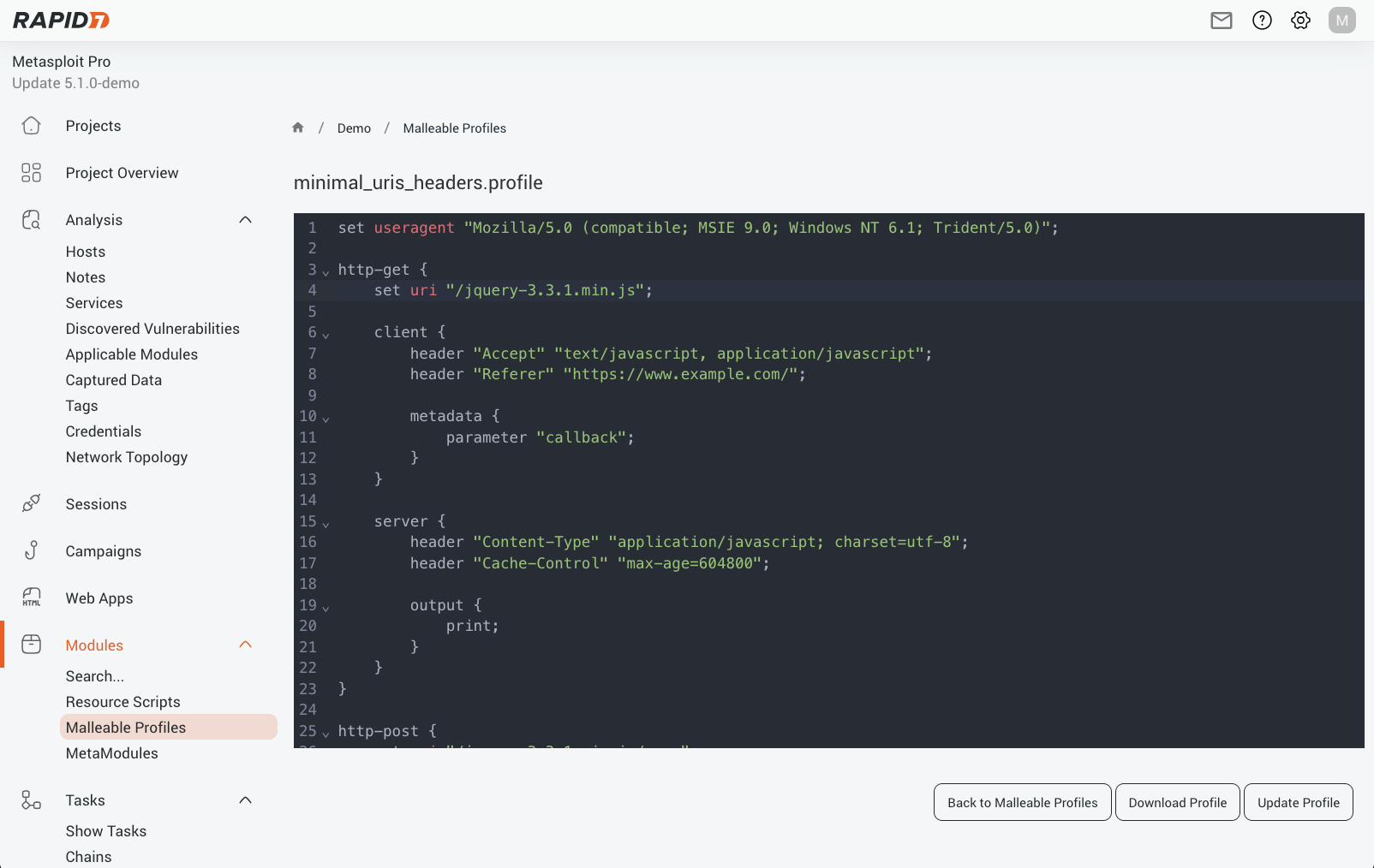
Figure 1 Malleable Profiles
Alongside the Malleable C2 integration, the payload selector has been overhauled across the Listener, Module Run, and Payload Generator pages. You can now filter payloads by platform and stage, making it much faster to find the right payload in large lists.
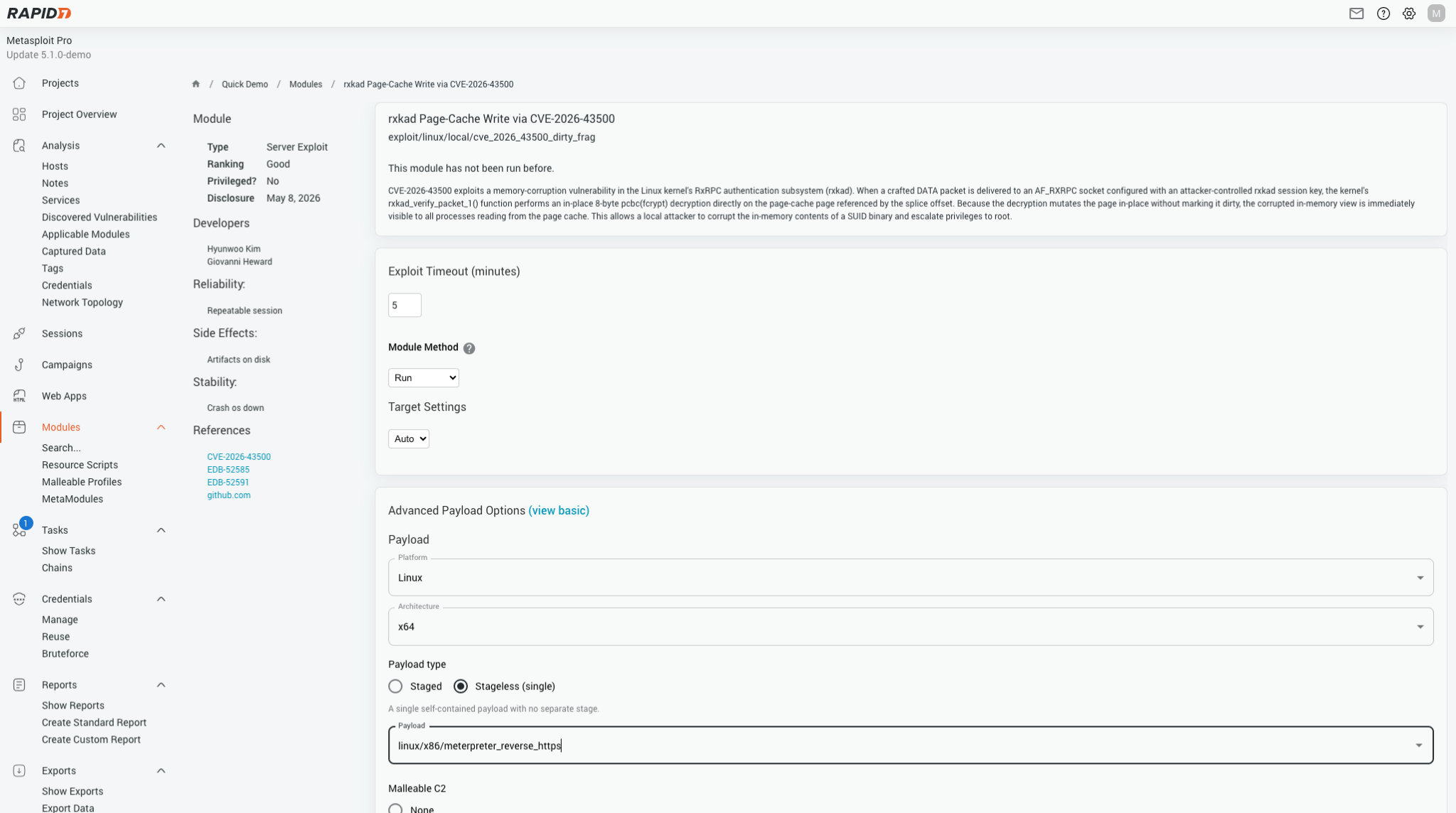
Figure 2: Advanced Payload Options
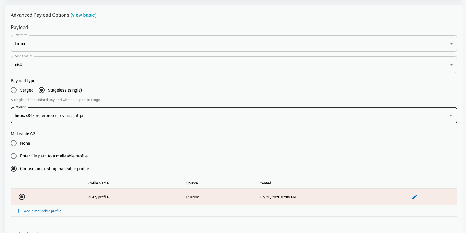
Figure 3: Additional Payload Options
The Discovered Services table has been overhauled with a cleaner, more capable interface consistent with the rest of Pro 5.1.
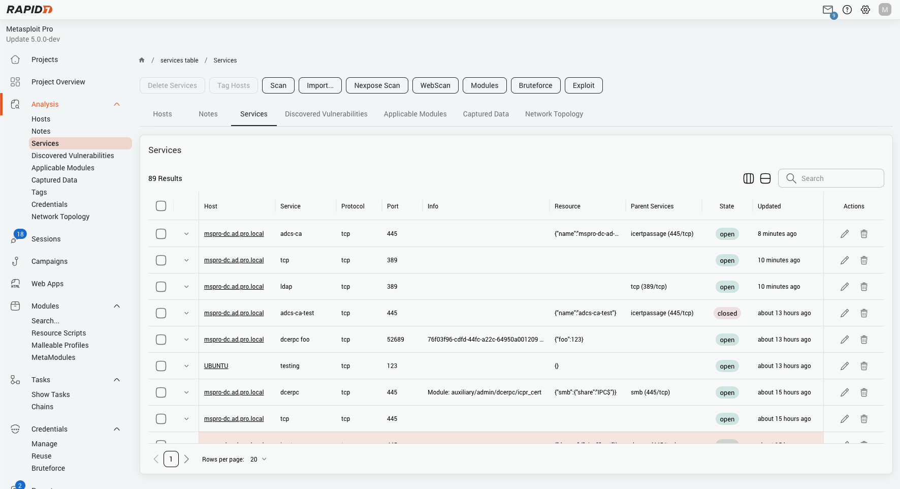
Figure 4: Service Options
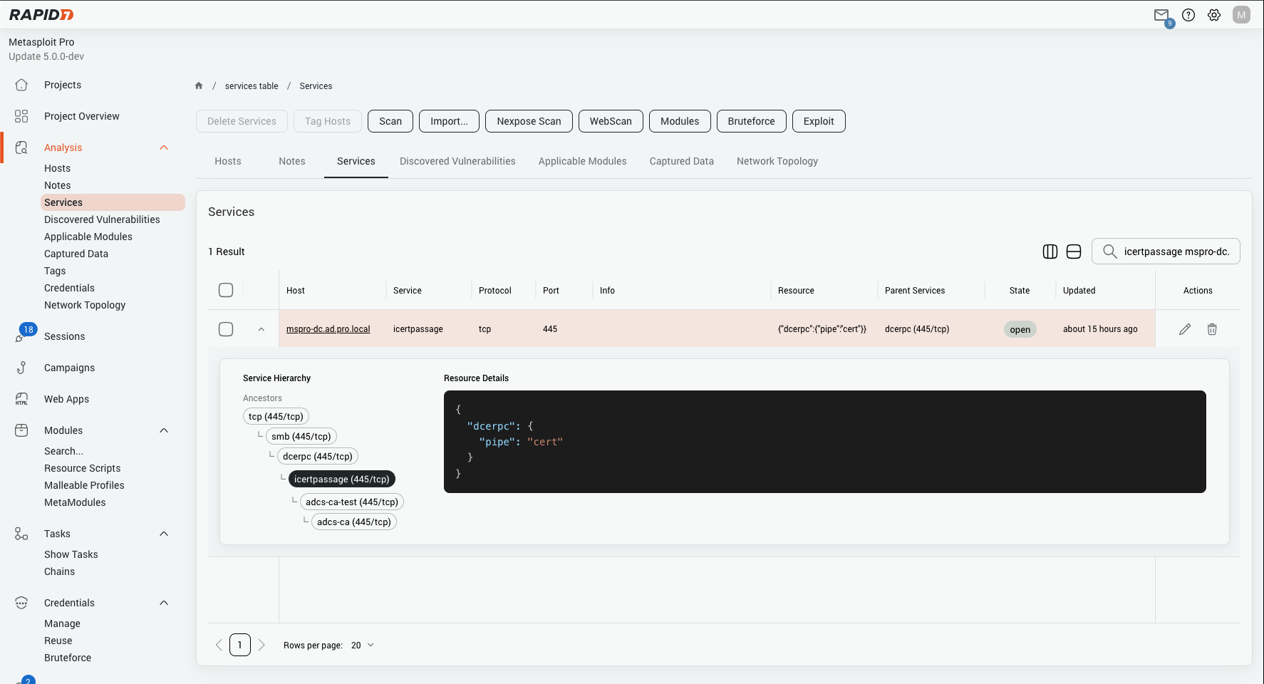
Figure 5: Service Hierarchy Display
Building on Metasploit Pro 5.0’s improvements to the Network Topology, we’ve added additional support and functionality for exploring your internal infrastructure. Previously, each node in the graph provided a high level summary of the host details when hovering over the node. This has now been moved into a dedicated side panel that surfaces everything you know about a host without leaving the topology view.
Click any node in the topology graph and the side panel now shows a consolidated summary of everything Metasploit knows about that host:
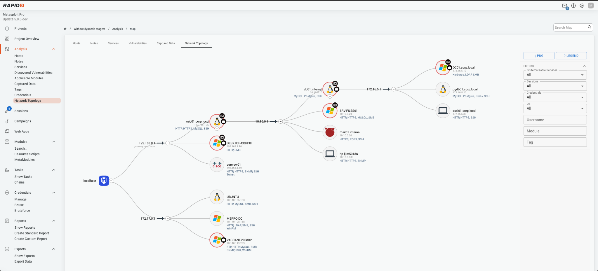
Figure 6: Network Topology Display
The topology graph toolbar has three new filters to help focus on the hosts that matter:
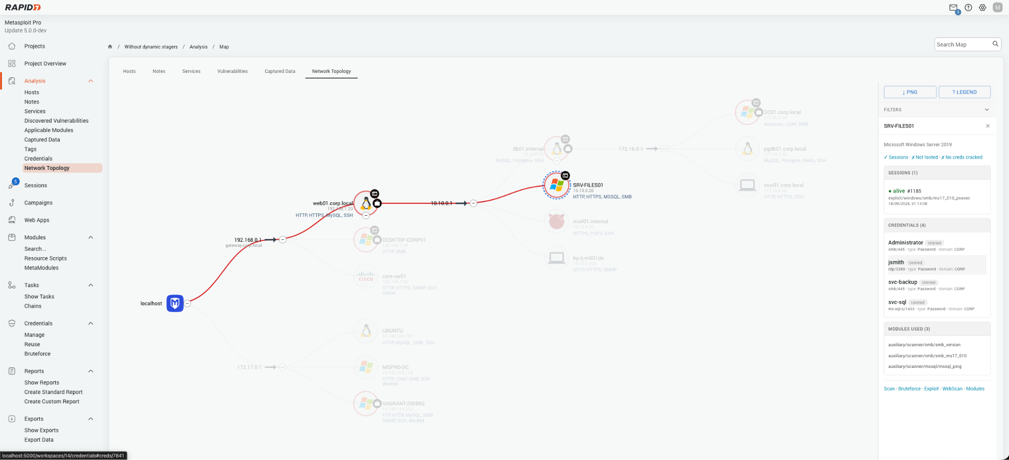
Figure 7: Network Topology Graph Filter Options
The Discovered Vulnerabilities table has been fully rewritten, bringing it in line with the UI overhaul introduced across the rest of Pro in 5.0.
Key improvements:
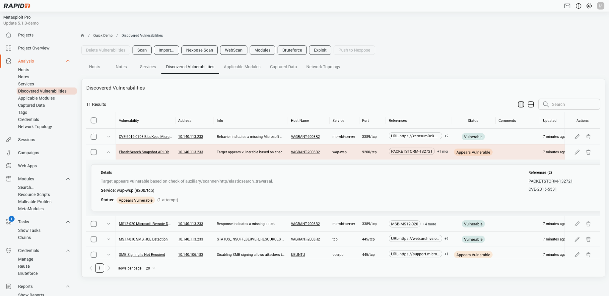
Figure 8: Discovered Vulnerabilities Modern UI
MITRE ATT&CK® is a globally-accessible knowledge base of adversary tactics and techniques based on real-world observations. The ATT&CK knowledge base is used as a foundation for the development of specific threat models and methodologies in the private sector, in government, and in the cybersecurity product and service community. Metasploit Pro now supports searching for modules by these techniques:
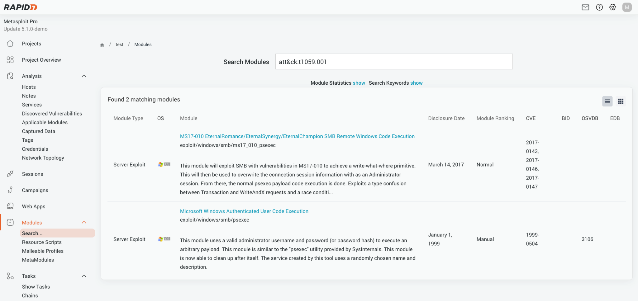
Figure 9: Attack Technique Filtering Search
Existing Pro installations can be upgraded through the standard update mechanism. Full upgrade instructions are available in the Metasploit Pro documentation.
These features are available in Metasploit Pro 5.1.0 onwards. We’re proud to collaborate with our customers, who are often the source of inspiration for product evolution. Ideas for improvements or enhancements can be shared with our Support team to help refine and submit them to the Product team on your behalf.
Post Syndicated from LastWeekTonight original https://www.youtube.com/shorts/Zl79TSscerI
Post Syndicated from jzb original https://lwn.net/Articles/1086900/
Greg Kroah-Hartman has announced the release of the 7.1.6, 6.18.42, 6.12.101, and 6.6.148 stable kernels. Each contains
hundreds of patches—the 7.1.6 kernel has more than
700—with fixes throughout the tree. Users are advised to
upgrade.
Post Syndicated from jzb original https://lwn.net/Articles/1086898/
The release of NetBSD 11.0, the 19th major version of the operating
system, has been announced. There are
many changes and enhancements since the 10.1 release, including a new
port to RISC-V, better support for Linux system calls in compat_linux(),
as well as improvements to the NPF
firewall.
As you are probably aware, the number of security issues found or
suspected everywhere has massively increased with the advent of AI
tools. As a consequence, we can’t publish a release without open
issues. Instead of delaying the release further to fix them (new ones
are being reported all the time), we’ve instead chosen to be
transparent about this.
See the full release
notes for links to the binary distributions and links to the full
change logs.
Post Syndicated from Matt Carey original https://blog.cloudflare.com/cloudflare-computer/
The most capable agents have something simple in common: they are given their own computer to work with.
Coding agents work this way. You give them a filesystem, a shell, tools, packages, and the ability to run code. They inspect the environment, make changes, test their work, and keep going. The computer gives the model a familiar way to act on the world. At Cloudflare, we’re working hard to provide the right primitives on which to build the most capable agents.
Today we’re introducing an early preview of @cloudflare/computer. The @cloudflare/computer package provides an agent runtime where the details and mechanics of what code runs in an isolate, a container sandbox, or a web browser are handled by the platform. Each agent gets a computer, the runtime optimizes for efficiency, and scalability.
We believe that in order to meet the growing demand for compute required by agentic systems we need to look to solutions beyond traditional containerization.
We’ve seen a subtle evolution of this story over the past six months. At the start of the year, spinning up a container and running an agent inside of it was the norm. In recent months, we’ve seen a rapid move for agent harnesses to provide sandboxed code execution via tools. This separates the hands (the sandbox where work is done) from the brain (the agent loop).
No matter where the harness runs, giving every agent a container presents a challenge — across all the clouds, all the hyperscalers, there’s nowhere near enough compute in the world for every company to give each of their users’ agents their own containerized compute environment. This will not scale to hundreds of millions, then billions, of concurrent agents. This is why there is desperate, panicked industry demand for CPU compute, not just GPU compute.
We’ve been working on this problem for a long time at Cloudflare, creating a more efficient compute primitive: isolates. We made that out-of-consensus bet almost 10 years ago when we introduced Cloudflare Workers. We made it again when we introduced Durable Objects almost six years ago. We made this bet because isolates are infinitely horizontally scalable. They spin up and tear down incredibly quickly. They can hibernate when the agent is idle, store the agent’s own state, and even spin up their own isolates to run untrusted code. Isolates are the best way to scale horizontally, and horizontal scale is what agents demand.
Last year, we gave isolates the ability to spin up their own container sandboxes. From day one, Cloudflare’s architecture has been designed to run the agent harness in the isolate (in a Durable Object) and call an attached container on-demand as a tool. This allows you to utilize heavier compute primitives only when required, optimizing performance and cost. Durable Objects scale infinitely horizontally, and the attached container lets it scale vertically to perform any task. This is how we build agents ourselves, and we’re seeing customers build incredible things this way too.
But when we look at this need to have multiple underlying compute primitives to build agents (isolates and containers) and the need for our customers and developers to combine them themselves in userspace, we think we can do better. We think that we can provide a simpler abstraction.
That’s why we’re starting this experiment by shipping @cloudflare/computer as an open-source library, to learn with our customers who are pushing the bounds of running agents at scale.
The @cloudflare/computer package starts with a simple premise: what if we give an agent a primed filesystem, declaratively defined, containing everything required for the task at hand and a selection of execution environments to operate on those files, each with their own pros and cons regarding speed, capability and cost?
It turns out that agents today are surprisingly capable of selecting the right environment for the task at hand. A job that only needs to manipulate files, process data, or manage a git repository can run inside an isolate. A command that needs Linux, npm, or a native binary can run inside a container. Both work against the same files that are kept in sync with the source filesystem.
The @cloudflare/computer package provides a durable filesystem that you can use with git repositories, storage buckets or any files you choose. It provides tools that let you read, write and edit files using Code Mode or bash commands. All operations are gated, audited and observed, giving you fine-grained control over changes the agent is allowed to perform as well as a clear paper trail showing what the agent did.
An instance of a @cloudflare/computer workspace can be instantiated on any Durable Object to provide a virtual filesystem and execution runtime.
It is installed via npm:
The primary use case is provide that filesystem and tooling to an agent. For example, here’s how to instantiate the workspace on an agent powered by @cloudflare/think intended to triage bug reports.
Several execution backends are provided as part of the @cloudflare/computer package, or you can write your own. Here we wire up a Cloudflare Container.
Expose the file, git, and shell tools alongside product specific tools to reply to reported issues.
The model can use tools during the agent loop, but you can also use the workspace API directly, for example, to prepare the environment before prompting the agent.
Check out the workspace repository for more examples of how to use the different backends and tools including a step-by-step tutorial walking through building an agent from scratch.
The central piece of @cloudflare/computer is the workspace. A virtual filesystem backed by SQLite that can be populated from various sources including cloud storage and source control.
The workspace supports optional execution runtimes that allow code to be run against the file system. All runtimes support the same interface exec(string, options) and currently two are provided out of the box (but you can write your own):
The Workspace class provides an API interface for manipulating the filesystem directly as well as a node:fs compatible wrapper so that it can be used easily with third-party JavaScript libraries.
For use with agents, we provide an AI SDK compatible toolkit that provides the most common tools: read, write, edit, ls and exec. The exec tool is a little special as it works across the runtimes taking a backend argument. The tool description guides the agent into choosing the correct runtime for the task at hand: either a fast, cheap worker backend or the fully featured container. In our testing, the frontier models are very good at making the correct decision and falling back to using containers only when needed.
Here at Cloudflare we’re already seeing agents exclusively using isolates to build, test, and deploy JavaScript applications with modern tooling, generate tailored documentation for each of our customers, and use web browsers to perform complex tasks.
Our goal with @cloudflare/computer is to provide an agent with a runtime where a container is required for less than 10% of its work, and coding tasks, audio/video manipulation, and document creation can all be handled by isolates.
Try out the early preview today – we can’t wait to hear your thoughts.
Post Syndicated from jzb original https://lwn.net/Articles/1086897/
Security updates have been issued by AlmaLinux (.NET 10.0, .NET 8.0, .NET 9.0, fence-agents, kernel, kernel-rt, openssh, osbuild-composer, perl-Archive-Tar, perl-DBI, perl:5.32, pipewire, python-pillow, qemu-kvm, unbound, and vim), Debian (chromium, incus, kernel, kissfft, libgd2, libmodbus, libssh, node-tar, php8.4, poppler, python-authlib, sslh, and starlette), Fedora (borgbackup, coturn, curl, exim, fuse-overlayfs, gh, GitPython, goaccess, lemonldap-ng, libgit2, nextcloud, nsd, php, postgresql16, python3.12, rabbitmq-server, rust-libgit2-sys, and xen), Mageia (bluez, firmware, kernel, kmod, wireless-regdb), Oracle (buildah, compat-libtiff3, dovecot, fence-agents, firefox, gimp, glibc, grafana, gstreamer1-plugins-bad-free, java-25-openjdk, kernel, libgcrypt, libtiff, libXfont2, nodejs24, nodejs:22, nodejs:24, openssh, openssl, PackageKit, pipewire, python-pillow, rest, sssd, vim, and yelp), SUSE (bind, chromium, dnsdist, gdk-pixbuf-loader-libheif, gio-branding-upstream, google-guest-agent, govulncheck-vulndb, GraphicsMagick, ignition, ImageMagick, keybase-client, kronosnet, libblkid-devel, libntpc1, libpng16, nano, openssh, openssl-1_0_0, openssl-3, openvpn, PackageKit, perl-mojolicious, php8, python-nltk, python313-asteval, python313-certifi, python313-GitPython, python313-huggingface-hub, rsyslog, tomcat, tomcat10, tomcat11, traefik2, valkey, warewulf4, webkit2gtk3, and yq), and Ubuntu (linux-intel-iotg).
Post Syndicated from Mar Witek original https://blog.cloudflare.com/grpc-workers/
AI is changing how people interact with computers, and voice is becoming an increasingly important part of that shift. Real-time assistants, AI-powered dictation, and other voice interfaces need low-latency communication between clients, models, and supporting services. Many developers use gRPC, a Remote Procedure Call (RPC) framework built on HTTP/2 and TCP, for this infrastructure.
Ever since Workers launched in 2017, we’ve been expanding their capabilities, including adding the ability to open outbound TCP connections and a JavaScript-native RPC system built on Cap’n Proto. And so as part of Agents Week, we’re extending Workers in the other direction, supporting inbound TCP connections and adding new ways to run gRPC applications on Cloudflare.
Today, we’re announcing:
We’re introducing this in private beta — you can sign up here.
Let’s dig into each of these below.
The Workers runtime now provides a connect() handler that accepts a socket that you can read from and write to:
You can pass this socket from one Worker to another Worker, or from a Worker to a Durable Object. This lets your Worker control where an incoming TCP connection is routed:
You can pass a socket from a Durable Object to its Container:
And then handle the socket in the container:
This gives you full control over the entire path from client to your server running in a container on Cloudflare, opening the door to full-duplex communication between client and server running any program, in any language, for any TCP-based protocol.
To expose the raw TCP socket to the client, we’re introducing a new type of Spectrum application, where you specify a Worker that you want incoming TCP connections to be routed to. Spectrum is Cloudflare’s ingress proxy for non-HTTP traffic, and allows Cloudflare to sit in front of any TCP or UDP application.
gRPC is a well-established and popular Remote Procedure Call (RPC) framework that was initially released by Google almost 10 years ago, and is now used across mobile apps, distributed systems, and most recently — voice AI applications.
Real-time voice AI applications demand low-latency, and both client and server to be able to send messages to each other over a single, persistent connection. WebSockets and Durable Objects are excellent fits for this, and the Cloudflare Agents SDK provides @cloudflare/voice to make this easy. But there is a ton of software out there that uses gRPC for real-time client-server communication.
Using the APIs described above, you can now deploy gRPC servers to Cloudflare, written in any language, with full support for bidirectional streaming between client and server. This lets you take advantage of Cloudflare’s network of 330+ locations and handle requests much closer to clients than is possible elsewhere. We’re excited about the doors this opens up for low-latency voice and colocated inference.
For example, here’s a minimal gRPC server that echoes messages it receives back to the client:
With this, there’s pretty much no gRPC-based application that you can’t deploy to Cloudflare, no matter what language it’s in or dependencies it relies on. But what if you need to do something simpler, and just serve a basic gRPC server or connect from a Worker to a gRPC server running somewhere else?
gRPC-web is a browser-compatible version of gRPC. Web browsers don’t expose the lower-level HTTP/2 features that gRPC requires, and there is no raw TCP Socket API built into web browsers — this is why the WebSocket API exists, and why Workers have supported WebSockets since 2021.
HTTP/2 splits each request and response into small binary messages called frames. This is core to how a single HTTP/2 or HTTP/3 connection is able to multiplex — many requests can be interleaved over one connection. Each frame has a stream ID, allowing the receiver to reassemble it into the correct request or response. gRPC depends on this stream-level control for efficient streaming, cancellation, flow control, and trailers.
Web platform APIs like fetch() don’t provide this control. So how can we make it simple and easy to use gRPC from Cloudflare Workers — without clients needing to make any changes? We translate incoming gRPC to gRPC-web, and translate outgoing gRPC-web to gRPC.
We’ve actually used gRPC-web within Cloudflare’s reverse proxy since 2020, when we wrote about the Road to gRPC on the Cloudflare blog. We convert requests to HTTP/1.1 so that messages can be inspected and gRPC apps can benefit from Cloudflare’s security features, like WAF rules and Bot Management.
Now, in private beta and then rolling out to everyone, we’re extending this so that given a Protocol Buffer (protobuf) definition file like this:
You can write a unary gRPC server in a Worker in just a few lines of code, using the @connectrpc/connect open-source package:
You can make outbound requests to external gRPC servers this way too, by using the client built into @connectrpc/connect:
Your code uses gRPC-web, but when it speaks to the outside world, it is automatically translated into gRPC. This means that clients and servers that you already depend on don’t need to change. For example, you can:
We’re introducing everything from this post in private beta — you can sign up here.
At Cloudflare, we use Cap’n Proto and Cap’n Web and the JavaScript-native RPC system that is built into Cloudflare Workers instead of gRPC. And when we ship things, we always aim to be using them ourselves. So in this case, we want to first work closely with a smaller set of developers using gRPC, and make sure we’ve nailed it before turning this on for everyone.
More broadly, we’re excited to continue to push the bounds of what types of traffic the Workers platform can serve, going beyond TCP and into UDP-based protocols. Keep telling us what you want to build on Workers, and we’ll keep pushing the bounds of what is possible.
Post Syndicated from Ryan Noel original https://blog.cloudflare.com/billable-usage-api/
Agents Week is about the shift already underway: agents write code, deploy Workers, and provision infrastructure on your behalf. That shift changes what you need to see. If a program is spending money in your Cloudflare account, you need to know what it's spending; throughout the day, per product, in a shape another program can consume. The dashboard is the right answer for humans. It's not the right answer for automation.
So we're launching a new Billable Usage API for self-serve accounts: a single endpoint that returns your account's usage and cost, broken down by product and by service period. It covers every usage-based Cloudflare product on the account, including Workers, R2, D1, Workers AI, Vectorize, Images, and Stream, all with one call. And if you already work in a FinOps toolchain, the column names should look familiar.
You'll get back an HTTP 200 OK with Content-Type: application/json and the usage rows in the response body. Today, usage and cost data are updated daily while we work towards providing more real time data.
Each row in the response is one charge period for one product on your account.
ServiceName and ServiceFamilyName — which product ("Workers Standard" under the "Workers" family, "R2 Storage" under "R2", etc.).ChargePeriodStart / ChargePeriodEnd — the window this row covers.PricingQuantity and ConsumedUnit — how much you used, in the unit of measure we bill on (GB-months, GB-seconds, requests, etc.).ContractedCost — what that period cost, in BillingCurrency.CumulatedPricingQuantity and CumulatedContractedCost — running totals for the billing period.ZoneId / ZoneName — when the usage is attributed to a specific zone.Most of these map directly to columns in the FinOps Open Cost and Usage Specification (FOCUS), so if your team is already ingesting FOCUS data from another provider, the names and semantics should be familiar:
Responses use the standard Cloudflare API envelope — result is an array of rows, one per product per charge period, alongside success, errors, and messages.
Matching FOCUS naming was a deliberate choice. AWS, Azure, Google Cloud, Oracle, and a growing list of SaaS providers already publish FOCUS formatted exports, and every serious cost-management tool speaks to it. That said, we're not yet claiming full conformance: a handful of columns the spec requires aren't in the payload today. Getting there is on our roadmap. Consider this the first step: familiar shape now, full conformance next.
We've partnered with Vantage on a native Cloudflare integration. Vantage is an infrastructure cost management platform that ingests cost and usage data from more than 30 providers, across AI, Cloud and SaaS providers, and brings it into a single view for reporting, allocation, and optimization. With this integration, your usage flows into the same Cost Reports, Budgets, and Cost Alerts you already use for the rest of your infrastructure.
Vantage connects to Cloudflare using a read-only API token with Billing Read access. Once connected, Vantage pulls your Billable Usage data daily and breaks it down by product (such as Workers and R2), zone, and account, so you can see which products drive your spend and attribute it to the teams and services behind it.
A few of the workflows this integration supports:
Connect your Cloudflare account in the Vantage console, and your costs appear next to everything else you run. There are no manual exports, no invoice uploads, and no separate dashboard to maintain.
This FOCUS standardized API also works with other Fintech tooling.
Agents do more than write code. They deploy Workers, provision R2 buckets, and manage D1 databases. When you grant programmatic access to your Cloudflare account, you need programmatic visibility into what it's costing you. Not at the end of the month, but throughout the day, by product, in a shape a program can actually consume.
The Billable Usage API is that shape. And customers have been asking us for programmatic usage for years. Finance teams want to pull spend into their own systems and attribute cost back to internal projects, teams, and even their end customers. Developers want a curl they can drop in a script. Every one of those workflows used to involve a screenshot or a manual export. Now it's an HTTP call, or a configuration in Vantage.
CumulatedContractedCost tells you where your spend is in the current billing cycle. We want to help you predict where you're going to end up. And not just at the account level, but the product level.The endpoint is live today for all self-serve accounts. Grab an API token with the Billing Read permission, point your curl at it, and you'll get back your current billing period broken down by product. Full reference is available on the Cloudflare API docs. To see it alongside the rest of your cloud spend, connect your Cloudflare account in the Vantage console.
Cloudflare has spent years making it easy to run more of your stack on our network. It's time we made it just as easy to see what that's costing you — on Cloudflare, and everywhere else.
Post Syndicated from Alex Reneau original https://blog.cloudflare.com/smaller-faster-safer-models/
Workers AI runs inference for some of the best open models in the world on GPUs in Cloudflare data centers close to your users. Two of the most capable, and most demanding, are Moonshot's Kimi K-series and Z.ai's GLM. They are large, long-context, mixture-of-experts models, and they are wonderful to use. They are also very hard to serve efficiently because of memory constraints.
We've written before about how we serve large models on Workers AI and about separating the prefill and decode phases of inference to get more out of each GPU. This post looks at three techniques we layer on top of that to fit these models into memory and keep them fast: quantizing the KV cache, compressing the model weights, and, because both of those pack more requests onto shared hardware, protecting the cache those requests share. These optimizations enable us to support more customers at lower costs, with no change in model accuracy.
All our experiments and production traffic are running and benchmarked with SGLang, an open-source inference serving framework. We found that SGLang offers the best performance in the market, and we work closely with the SGLang team to upstream patches and new features to make our work available to the open-source community.
As a model generates text, it stores the attention keys (K) and values (V) for every token it has already processed in a structure called the KV cache. The cache is what lets the model extend a long conversation without re-reading the entire context on every new token. For a long-context model, it grows quickly, and it is usually the KV cache, not the model's weights, that fills up GPU memory first.
By default, the cache is stored in 16-bit precision (BF16). We store it in 8-bit floating point instead (FP8, e4m3), which halves its size. On Kimi K2.6, that raises the amount of context we can hold in memory from roughly 686,000 tokens to about 1.37 million, twice as much.
It's worth being precise about where the benefit comes from, because it isn't raw speed. Quantizing the cache adds a small amount of work per token, since the FP8 attention kernel has to convert values as it reads them. What it changes is how many requests we can keep resident at once. The following measurements are for Kimi K2.6 decoding on a disaggregated H200 deployment, comparing the attention kernels directly:
At any single concurrency level, BF16 is a few percent faster per token. But BF16 runs out of cache at 32 concurrent requests and can't admit a 33rd, while FP8 keeps going to 64 and reaches 2,192 tokens per second, about 41% higher than BF16's peak, for roughly 30% less cost per token. Because we run prefill and decode as separate pools, we can apply this where it helps most: prefill is compute-bound rather than memory-bound, so there we leave the cache in BF16 and keep its slightly higher throughput.
None of this would matter if it changed the model's answers, so we checked. Across our evaluation suite, FP8 and BF16 caches are indistinguishable:
The KV cache is one demand on GPU memory; the model's weights are the other. For GLM 5.2, we compress the weights from 8-bit floating point down to 4-bit integers (INT4) with no loss in accuracy. The checkpoint shrinks from 705 GB to 421 GB, about 40%, and per-GPU memory across an 8-way tensor-parallel deployment drops from roughly 88 GB to 52 GB, which leaves room for around 1.18 million tokens of KV cache on the same hardware.
Across our evaluation suite, INT4 and FP8 weights are indistinguishable:
Smaller weights make the decode phase faster, and for a clear reason: generating each token means streaming the model's weights out of GPU memory, so decode speed is limited by memory bandwidth. Move less data and every token arrives sooner. The effect is largest at low concurrency, where per-request latency matters most:
Prefill behaves differently. It is compute-bound, and INT4 weights have to be expanded back out before the model can multiply with them, so that extra step makes prefill slower rather than faster, GLM sustains about 10,160 tokens per second of prefill in FP8 versus 8,660 in INT4. As with the KV cache, the disaggregated design turns this into a choice rather than a compromise: we run INT4 for decode, where it wins, and FP8 for prefill, where it wins. Model accuracy stays within 0.8 points of the FP8 model across every benchmark we run, making its quality indistinguishable.
Both techniques above have the same effect: they let many more requests share one GPU's memory at the same time. That efficiency is the whole point, but it also means hundreds of requests are reading and writing pages of the same physical KV cache. The mechanisms that make this fast, paged attention, continuous batching, cache reuse, all rely on getting the bookkeeping exactly right, and at our request volumes, even a one-in-a-billion mistake would show up regularly.
So we built KV cache integrity checking as a layer of defense. The idea is straightforward: every physical cache page gets a tag that changes whenever the page is reallocated, and the server records which pages and tags each request expects to use. Before supported decode operations read from the cache, those mappings are checked. If anything doesn't match, the affected request is aborted rather than allowed to return data from the wrong page.
The question that decides whether a safety check ships is what it costs. We measured it on a mid-sized production model in a two-prefill, two-decode configuration, with 8,192-token inputs and 1,000-token outputs:
The cost is under 1% on both throughput and tail latency, and even the upper bound of the 95% confidence interval stays near 1%. We kept it computationally cheap by running the validation as a separate batch check rather than fusing it into the attention kernel, which would have introduced a race between GPU thread groups. It's enabled per deployment, and the default path uses a no-op tracker with no measurable overhead, so deployments that don't need it pay nothing.
Serving frontier models efficiently is a moving target, and this is the ongoing work behind it. We're expanding FP8 KV caches across more of the fleet, validating NVFP4 weights on Blackwell (NVIDIA’s GPU architecture), and working toward making integrity checks something we can leave on everywhere at negligible cost. These optimizations will allow us to continue to support more customers at a lower cost and at the same accuracy.
If squeezing the best open models onto GPUs and serving them to millions of developers sounds like your kind of problem, come work with us.