Super Slurper is Cloudflare’s data migration tool that is designed to make large-scale data transfers between cloud object storage providers and Cloudflare R2 easy. Since its launch, thousands of developers have used Super Slurper to move petabytes of data from AWS S3, Google Cloud Storage, and other S3-compatible services to R2.
But we saw an opportunity to make it even faster. We rearchitected Super Slurper from the ground up using our Developer Platform — building on Cloudflare Workers, Durable Objects, and Queues — and improved transfer speeds by up to 5x. In this post, we’ll dive into the original architecture, the performance bottlenecks we identified, how we solved them, and the real-world impact of these improvements.
Initial architecture and performance bottlenecks
Super Slurper originally shared its architecture with SourcingKit, a tool built to bulk import images from AWS S3 into Cloudflare Images. SourcingKit was deployed on Kubernetes and ran alongside the Images service. When we started building Super Slurper, we split it into its own Kubernetes namespace and introduced a few new APIs to make it easier to use for the object storage use case. This setup worked well and helped thousands of developers move data to R2.
However, it wasn’t without its challenges. SourcingKit wasn’t designed to handle the scale required for large, petabytes-scale transfers. SourcingKit, and by extension Super Slurper, operated on Kubernetes clusters located in one of our core data centers, meaning it had to share compute resources and bandwidth with Cloudflare’s control plane, analytics, and other services. As the number of migrations grew, these resource constraints became a clear bottleneck.
For a service transferring data between object storage providers, the job is simple: list objects from the source, copy them to the destination, and repeat. This is exactly how the original Super Slurper worked. We listed objects from the source bucket, pushed that list to a Postgres-based queue (pg_queue), and then pulled from this queue at a steady pace to copy objects over. Given the scale of object storage migrations, bandwidth usage was inevitably going to be high. This made it challenging to scale.
To address the bandwidth constraints operating solely in our core data center, we introduced Cloudflare Workers into the mix. Instead of handling the copying of data in our core data center, we started calling out to a Worker to do the actual copying:
As Super Slurper’s usage grew, so did our Kubernetes resource consumption. A significant amount of time during data transfers was spent waiting on network I/O or storage, and not actually doing compute-intensive tasks. So we didn’t need more memory or more CPU, we needed more concurrency.
To keep up with demand, we kept increasing the replica count. But eventually, we hit a wall. We were dealing with scalability challenges when running on the order of tens of pods when we wanted multiple orders of magnitude more.
We decided to rethink the entire approach from first principles, instead of leaning on the architecture we had inherited. In about a week, we built a rough proof of concept using Cloudflare Workers, Durable Objects, and Queues. We listed objects from the source bucket, pushed them into a queue, and then consumed messages from the queue to initiate transfers. Although this sounds very similar to what we did in the original implementation, building on our Developer Platform allowed us to automatically scale an order of magnitude higher than before.
Cloudflare Queues: Enables asynchronous object transfers and auto-scales to meet the number of objects being migrated.
Cloudflare Workers: Runs lightweight compute tasks without the overhead of Kubernetes and optimizes where in the world each part of the process runsfor lower latency and better performance.
SQLite-backed Durable Objects (DOs): Acts as a fully distributed database, eliminating the limitations of a single PostgreSQL instance.
Hyperdrive: Provides fast access to historical job data from the original PostgreSQL database, keeping it as an archive store.
We ran a few tests and found that our proof of concept was slower than the original implementation for small transfers (a few hundred objects), but it matched and eventually exceeded the performance of the original as transfers scaled into the millions of objects. That was the signal we needed to invest the time to take our proof of concept to production.
We removed our proof of concept hacks, worked on stability, and found new ways to make transfers scale to even higher concurrency. After a few iterations, we landed on something we were happy with.
New architecture: Workers, Queues, and Durable Objects
Processing layer: managing the flow of migration
At the heart of our processing layer are queues, consumers, and workers. Here’s what the process looks like:
Kicking off a migration
When a client triggers a migration, it starts with a request sent to our API Worker. This worker takes the details of the migration, stores them in the database, and adds a message to the List Queue to start the process.
Listing source bucket objects
The List Queue Consumer is where things start to pick up. It pulls messages from the queue, retrieves object listings from the source bucket, applies any necessary filters, and stores important metadata in the database. Then, it creates new tasks by enqueuing object transfer messages into the Transfer Queue.
We immediately queue new batches of work, maximizing concurrency. A built-in throttling mechanism prevents us from adding more messages to our queues when unexpected failures occur, such as dependent systems going down. This helps maintain stability and prevents overload during disruptions.
Efficient object transfers
The Transfer Queue Consumer Workers pull object transfer messages from the queue, ensuring that each object is processed only once by locking the object key in the database. When the transfer finishes, the object is unlocked. For larger objects, we break them into manageable chunks and transfer them as multipart uploads.
Handling failures gracefully
Failures are inevitable in any distributed system, and we had to make sure we accounted for that. We implemented automatic retries for transient failures, so issues don’t interrupt the flow of the migration. But if something can’t be resolved with retries, the message goes into the Dead Letter Queue (DLQ), where it is logged for later review and resolution.
Job completion & lifecycle management
Once all the objects are listed and the transfers are in progress, the Lifecycle Queue Consumer keeps an eye on everything. It monitors the ongoing transfers, ensuring that no object is left behind. When all the transfers are complete, the job is marked as finished and the migration process wraps up.
Database layer: durable storage & legacy data retrieval
When building our new architecture, we knew we needed a robust solution to handle massive datasets while ensuring retrieval of historical job data. That’s where our combination of Durable Objects (DOs) and Hyperdrive came in.
Durable Objects
We gave each account a dedicated Durable Object to track migration jobs. Each job’s DO stores vital details, such as bucket names, user options, and job state. This ensured everything stayed organized and easy to manage. To support large migrations, we also added a Batch DO that manages all the objects queued for transfer, storing their transfer state, object keys, and any extra metadata.
As migrations scaled up to billions of objects, we had to get creative with storage. We implemented a sharding strategy to distribute request loads, preventing bottlenecks and working around SQLite DO’s 10 GB storage limit. As objects are transferred, we clean up their details, optimizing storage space along the way. It’s surprising how much storage a billion object keys can require!
Hyperdrive
Since we were rebuilding a system with years of migration history, we needed a way to preserve and access every past migration detail. Hyperdrive serves as a bridge to our legacy systems, enabling seamless retrieval of historical job data from our core PostgreSQL database. It’s not just a data retrieval mechanism, but an archive for complex migration scenarios.
Results: Super Slurper now transfers data to R2 up to 5x faster
So, after all of that, did we actually achieve our goal of making transfers faster?
We ran a test migration of 75,000 objects from AWS S3 to R2. With the original implementation, the transfer took 15 minutes and 30 seconds. After our performance improvements, the same migration completed in just 3 minutes and 25 seconds.
When production migrations started using the new service in February, we saw even greater improvements in some cases, especially depending on the distribution of object sizes. Super Slurper has been around for about two years. But the improved performance has led to it being able to move much more data — 35% of all objects copied by Super Slurper happened just in the last two months.
Challenges
One of the biggest challenges we faced with the new architecture was handling duplicate messages. There were a couple of ways duplicates could occur:
Queues provides at-least-once delivery, which means consumers may receive the same message more than once to guarantee delivery.
Failures and retries could also create apparent duplicates. For example, if a request to a Durable Object fails after the object has already been transferred, the retry could reprocess the same object.
If not handled correctly, this could result in the same object being transferred multiple times. To solve this, we implemented several strategies to ensure each object was accurately accounted for and only transferred once:
Since listing is sequential (e.g., to get object 2, you need the continuation token from listing object 1), we assign a sequence ID to each listing operation. This allows us to detect duplicate listings and prevent multiple processes from starting simultaneously. This is particularly useful because we don’t wait for database and queue operations to complete before listing the next batch. If listing 2 fails, we can retry it, and if listing 3 has already started, we can short-circuit unnecessary retries.
Each object is locked when its transfer begins, preventing parallel transfers of the same object. Once successfully transferred, the object is unlocked by deleting its key from the database. If a message for that object reappears later, we can safely assume it has already been transferred if the key no longer exists.
We rely on database transactions to keep our counts accurate. If an object fails to unlock, its count remains unchanged. Similarly, if an object key fails to be added to the database, the count isn’t updated, and the operation will be retried later.
As a last failsafe, we check whether the object already exists in the target bucket and was published after the start of our migration. If so, we assume it was transferred by our process (or another) and safely skip it.
What’s next for Super Slurper?
We’re always exploring ways to make Super Slurper faster, more scalable, and even easier to use — this is just the beginning.
Data migrations are still currently limited to 3 concurrent migrations per account, but we want to increase that limit. This will allow object prefixes to be split up into separate migrations and run in parallel, drastically increasing the speed at which a bucket can be migrated. For more information on Super Slurper and how to migrate data from existing object storage to R2, refer to our documentation.
P.S. As part of this update, we made the API much simpler to interact with, so migrations can now be managed programmatically!
Read replication of D1 databases is in public beta!
D1 read replication makes read-only copies of your database available in multiple regions across Cloudflare’s network. For busy, read-heavy applications like e-commerce websites, content management tools, and mobile apps:
D1 read replication lowers average latency by routing user requests to read replicas in nearby regions.
D1 read replication increases overall throughput by offloading read queries to read replicas, allowing the primary database to handle more write queries.
The main copy of your database is called the primary database and the read-only copies are called read replicas. When you enable replication for a D1 database, the D1 service automatically creates and maintains read replicas of your primary database. As your users make requests, D1 routes those requests to an appropriate copy of the database (either the primary or a replica) based on performance heuristics, the type of queries made in those requests, and the query consistency needs as expressed by your application.
All of this global replica creation and request routing is handled by Cloudflare at no additional cost.
To take advantage of read replication, your Worker needs to use the new D1 Sessions API. Click the button below to run a Worker using D1 read replication with this code example to see for yourself!
D1 Sessions API
D1’s read replication feature is built around the concept of database sessions. A session encapsulates all the queries representing one logical session for your application. For example, a session might represent all requests coming from a particular web browser or all requests coming from a mobile app used by one of your users. If you use sessions, your queries will use the appropriate copy of the D1 database that makes the most sense for your request, be that the primary database or a nearby replica.
The sessions implementation ensures sequential consistency for all queries in the session, no matter what copy of the database each query is routed to. The sequential consistency model has important properties like “read my own writes” and “writes follow reads,” as well as a total ordering of writes. The total ordering of writes means that every replica will see transactions committed in the same order, which is exactly the behavior we want in a transactional system. Said another way, sequential consistency guarantees that the reads and writes are executed in the order in which you write them in your code.
Some examples of consistency implications in real-world applications:
You are using an online store and just placed an order (write query), followed by a visit to the account page to list all your orders (read query handled by a replica). You want the newly placed order to be listed there as well.
You are using your bank’s web application and make a transfer to your electricity provider (write query), and then immediately navigate to the account balance page (read query handled by a replica) to check the latest balance of your account, including that last payment.
Why do we need the Sessions API? Why can we not just query replicas directly?
Applications using D1 read replication need the Sessions API because D1 runs on Cloudflare’s global network and there’s no way to ensure that requests from the same client get routed to the same replica for every request. For example, the client may switch from WiFi to a mobile network in a way that changes how their requests are routed to Cloudflare. Or the data center that handled previous requests could be down because of an outage or maintenance.
D1’s read replication is asynchronous, so it’s possible that when you switch between replicas, the replica you switch to lags behind the replica you were using. This could mean that, for example, the new replica hasn’t learned of the writes you just completed. We could no longer guarantee useful properties like “read your own writes”. In fact, in the presence of shifty routing, the only consistency property we could guarantee is that what you read had been committed at some point in the past (read committed consistency), which isn’t very useful at all!
Since we can’t guarantee routing to the same replica, we flip the script and use the information we get from the Sessions API to make sure whatever replica we land on can handle the request in a sequentially-consistent manner.
Here’s what the Sessions API looks like in a Worker:
export default {
  async fetch(request: Request, env: Env) {
    // A. Create the session.
    // When we create a D1 session, we can continue where we left off from a previous
    // session if we have that session's last bookmark or use a constraint.
    const bookmark = request.headers.get('x-d1-bookmark') ?? 'first-unconstrained'
    const session = env.DB.withSession(bookmark)

    // Use this session for all our Workers' routes.
    const response = await handleRequest(request, session)

    // B. Return the bookmark so we can continue the session in another request.
    response.headers.set('x-d1-bookmark', session.getBookmark())

    return response
  }
}

async function handleRequest(request: Request, session: D1DatabaseSession) {
  const { pathname } = new URL(request.url)

  if (request.method === "GET" && pathname === '/api/orders') {
    // C. Session read query.
    const { results } = await session.prepare('SELECT * FROM Orders').all()
    return Response.json(results)

  } else if (request.method === "POST" && pathname === '/api/orders') {
    const order = await request.json<Order>()

    // D. Session write query.
    // Since this is a write query, D1 will transparently forward it to the primary.
    await session
      .prepare('INSERT INTO Orders VALUES (?, ?, ?)')
      .bind(order.orderId, order.customerId, order.quantity)
      .run()

    // E. Session read-after-write query.
    // In order for the application to be correct, this SELECT statement must see
    // the results of the INSERT statement above.
    const { results } = await session
      .prepare('SELECT * FROM Orders')
      .all()

    return Response.json(results)
  }

  return new Response('Not found', { status: 404 })
}
To use the Session API, you first need to create a session using the withSession method (step A). The withSession method takes a bookmark as a parameter, or a constraint. The provided constraint instructs D1 where to forward the first query of the session. Using first-unconstrained allows the first query to be processed by any replica without any restriction on how up-to-date it is. Using first-primary ensures that the first query of the session will be forwarded to the primary.
// A. Create the session.
const bookmark = request.headers.get('x-d1-bookmark') ?? 'first-unconstrained'
const session = env.DB.withSession(bookmark)
Providing an explicit bookmark instructs D1 that whichever database instance processes the query has to be at least as up-to-date as the provided bookmark (in case of a replica; the primary database is always up-to-date by definition). Explicit bookmarks are how we can continue from previously-created sessions and maintain sequential consistency across user requests.
Once you’ve created the session, make queries like you normally would with D1. The session object ensures that the queries you make are sequentially consistent with regards to each other.
// C. Session read query.
const { results } = await session.prepare('SELECT * FROM Orders').all()
For example, in the code example above, the session read query for listing the orders (step C) will return results that are at least as up-to-date as the bookmark used to create the session (step A).
More interesting is the write query to add a new order (step D) followed by the read query to list all orders (step E). Because both queries are executed on the same session, it is guaranteed that the read query will observe a database copy that includes the write query, thus maintaining sequential consistency.
// D. Session write query.
await session
  .prepare('INSERT INTO Orders VALUES (?, ?, ?)')
  .bind(order.orderId, order.customerId, order.quantity)
  .run()

// E. Session read-after-write query.
const { results } = await session
  .prepare('SELECT * FROM Orders')
  .all()
Note that we could make a single batch query to the primary including both the write and the list, but the benefit of using the new Sessions API is that you can use the extra read replica databases for your read queries and allow the primary database to handle more write queries.
The session object does the necessary bookkeeping to maintain the latest bookmark observed across all queries executed using that specific session, and always includes that latest bookmark in requests to D1. Note that any query executed without using the session object is not guaranteed to be sequentially consistent with the queries executed in the session.
When possible, we suggest continuing sessions across requests by including bookmarks in your responses to clients (step B), and having clients passing previously received bookmarks in their future requests.
// B. Return the bookmark so we can continue the session in another request.
response.headers.set('x-d1-bookmark', session.getBookmark())
This allows all of a client’s requests to be in the same session. You can do this by grabbing the session’s current bookmark at the end of the request (session.getBookmark()) and sending the bookmark in the response back to the client in HTTP headers, in HTTP cookies, or in the response body itself.
Consistency with and without Sessions API
In this section, we will explore the classic scenario of a read-after-write query to showcase how using the new D1 Sessions API ensures that we get sequential consistency and avoid any issues with inconsistent results in our application.
The Client, a user Worker, sends a D1 write query that gets processed by the database primary and gets the results back. However, the subsequent read query ends up being processed by a database replica. If the database replica is lagging far enough behind the database primary, such that it does not yet include the first write query, then the returned results will be inconsistent, and probably incorrect for your application business logic.
Using the Sessions API fixes the inconsistency issue. The first write query is again processed by the database primary, and this time the response includes “Bookmark 100”. The session object will store this bookmark for you transparently.
The subsequent read query is processed by database replica as before, but now since the query includes the previously received “Bookmark 100”, the database replica will wait until its database copy is at least up-to-date as “Bookmark 100”. Only once it’s up-to-date, the read query will be processed and the results returned, including the replica’s latest bookmark “Bookmark 104”.
Notice that the returned bookmark for the read query is “Bookmark 104”, which is different from the one passed in the query request. This can happen if there were other writes from other client requests that also got replicated to the database replica in-between the two queries our own client executed.
Enabling read replication
To start using D1 read replication:
Update your Worker to use the D1 Sessions API to tell D1 what queries are part of the same database session. The Sessions API works with databases that do not have read replication enabled as well, so it’s safe to ship this code even before you enable replicas. Here’s an example.
D1 read replication is built into D1, and you don’t pay extra storage or compute costs for replicas. You incur the exact same D1 usage with or without replicas, based on rows_read and rows_written by your queries. Unlike other traditional database systems with replication, you don’t have to manually create replicas, including where they run, or decide how to route requests between the primary database and read replicas. Cloudflare handles this when using the Sessions API while ensuring sequential consistency.
Since D1 read replication is in beta, we recommend trying D1 read replication on a non-production database first, and migrate to your production workloads after validating read replication works for your use case.
If you don’t have a D1 database and want to try out D1 read replication, create a test database in the Cloudflare dashboard.
Observing your replicas
Once you’ve enabled D1 read replication, read queries will start to be processed by replica database instances. The response of each query includes information in the nested meta object relevant to read replication, like served_by_region and served_by_primary. The first denotes the region of the database instance that processed the query, and the latter will be true if-and-only-if your query was processed by the primary database instance.
In addition, the D1 dashboard overview for a database now includes information about the database instances handling your queries. You can see how many queries are handled by the primary instance or by a replica, and a breakdown of the queries processed by region. The example screenshots below show graphs displaying the number of queries executed and number of rows read by each region.
Under the hood: how D1 read replication is implemented
D1 is implemented on top of SQLite-backed Durable Objects running on top of Cloudflare’s Storage Relay Service.
D1 is structured with a 3-layer architecture. First is the binding API layer that runs in the customer’s Worker. Next is a stateless Worker layer that routes requests based on database ID to a layer of Durable Objects that handle the actual SQL operations behind D1. This is similar to how most applications using Cloudflare Workers and Durable Objects are structured.
For a non-replicated database, there is exactly one Durable Object per database. When a user’s Worker makes a request with the D1 binding for the database, that request is first routed to a D1 Worker running in the same location as the user’s Worker. The D1 Worker figures out which D1 Durable Object backs the user’s D1 database and fetches an RPC stub to that Durable Object. The Durable Objects routing layer figures out where the Durable Object is located, and opens an RPC connection to it. Finally, the D1 Durable Object then handles the query on behalf of the user’s Worker using the Durable Objects SQL API.
In the Durable Objects SQL API, all queries go to a SQLite database on the local disk of the server where the Durable Object is running. Durable Objects run SQLite in WAL mode. In WAL mode, every write query appends to a write-ahead log (the WAL). As SQLite appends entries to the end of the WAL file, a database-specific component called the Storage Relay Service leader synchronously replicates the entries to 5 durability followers on servers in different datacenters. When a quorum (at least 3 out of 5) of the durability followers acknowledge that they have safely stored the data, the leader allows SQLite’s write queries to commit and opens the Durable Object’s output gate, so that the Durable Object can respond to requests.
Our implementation of WAL mode allows us to have a complete log of all of the committed changes to the database. This enables a couple of important features in SQLite-backed Durable Objects and D1:
We construct databases anywhere in the world by downloading all of the WAL entries from cold storage and replaying each WAL entry in order.
We implement Point-in-time recovery (PITR) by replaying WAL entries up to a specific bookmark rather than to the end of the log.
Unfortunately, having the main data structure of the database be a log is not ideal. WAL entries are in write order, which is often neither convenient nor fast. In order to cut down on the overheads of the log, SQLite checkpoints the log by copying the WAL entries back into the main database file. Read queries are serviced directly by SQLite using files on disk — either the main database file for checkpointed queries, or the WAL file for writes more recent than the last checkpoint. Similarly, the Storage Relay Service snapshots the database to cold storage so that we can replay a database by downloading the most recent snapshot and replaying the WAL from there, rather than having to download an enormous number of individual WAL entries.
WAL mode is the foundation for implementing read replication, since we can stream writes to locations other than cold storage in real time.
We implemented read replication in 5 major steps.
First, we made it possible to make replica Durable Objects with a read-only copy of the database. These replica objects boot by fetching the latest snapshot and replaying the log from cold storage to whatever bookmark primary database’s leader last committed. This basically gave us point-in-time replicas, since without continuous updates, the replicas never updated until the Durable Object restarted.
Second, we registered the replica leader with the primary’s leader so that the primary leader sends the replicas every entry written to the WAL at the same time that it sends the WAL entries to the durability followers. Each of the WAL entries is marked with a bookmark that uniquely identifies the WAL entry in the sequence of WAL entries. We’ll use the bookmark later.
Note that since these writes are sent to the replicas before a quorum of durability followers have confirmed them, the writes are actually unconfirmed writes, and the replica leader must be careful to keep the writes hidden from the replica Durable Object until they are confirmed. The replica leader in the Storage Relay Service does this by implementing enough of SQLite’s WAL-index protocol, so that the unconfirmed writes coming from the primary leader look to SQLite as though it’s just another SQLite client doing unconfirmed writes. SQLite knows to ignore the writes until they are confirmed in the log. The upshot of this is that the replica leader can write WAL entries to the SQLite WAL immediately, and then “commit” them when the primary leader tells the replica that the entries have been confirmed by durability followers.
One neat thing about this approach is that writes are sent from the primary to the replica as quickly as they are generated by the primary, helping to minimize lag between replicas. In theory, if the write query was proxied through a replica to the primary, the response back to the replica will arrive at almost the same time as the message that updates the replica. In such a case, it looks like there’s no replica lag at all!
In practice, we find that replication is really fast. Internally, we measure confirm lag, defined as the time from when a primary confirms a change to when the replica confirms a change. The table below shows the confirm lag for two D1 databases whose primaries are in different regions.
Replica Region
Database A
(Primary region: ENAM)
Database B (Primary region: WNAM)
ENAM
N/A
30 ms
WNAM
45 ms
N/A
WEUR
55 ms
75 ms
EEUR
67 ms
75 ms
Confirm lag for 2 replicated databases. N/A means that we have no data for this combination. The region abbreviations are the same ones used for Durable Object location hints.
The table shows that confirm lag is correlated with the network round-trip time between the data centers hosting the primary databases and their replicas. This is clearly visible in the difference between the confirm lag for the European replicas of the two databases. As airline route planners know, EEUR is appreciably further away from ENAM than WNAM, but from WNAM, both European regions (WEUR and EEUR) are about equally as far away. We see that in our replication numbers.
The exact placement of the D1 database in the region matters too. Regions like ENAM and WNAM are quite large in themselves. Database A’s placement in ENAM happens to be further away from most data centers in WNAM compared to database B’s placement in WNAM relative to the ENAM data centers. As such, database B sees slightly lower confirm lag.
Try as we might, we can’t beat the speed of light!
Third, we updated the Durable Object routing system to be aware of Durable Object replicas. When read replication is enabled on a Durable Object, two things happen. First, we create a set of replicas according to a replication policy. The current replication policy that D1 uses is simple: a static set of replicas in every region that D1 supports. Second, we turn on a routing policy for the Durable Object. The current policy that D1 uses is also simple: route to the Durable Object replica in the region close to where the user request is. With this step, we have updateable read-only replicas, and can route requests to them!
Fourth, we updated D1’s Durable Object code to handle write queries on replicas. D1 uses SQLite to figure out whether a request is a write query or a read query. This means that the determination of whether something is a read or write query happens after the request is routed. Read replicas will have to handle write requests! We solve this by instantiating each replica D1 Durable Object with a reference to its primary. If the D1 Durable Object determines that the query is a write query, it forwards the request to the primary for the primary to handle. This happens transparently, keeping the user code simple.
As of this fourth step, we can handle read and write queries at every copy of the D1 Durable Object, whether it’s a primary or not. Unfortunately, as outlined above, if a user’s requests get routed to different read replicas, they may see different views of the database, leading to a very weak consistency model. So the last step is to implement the Sessions API across the D1 Worker and D1 Durable Object. Recall that every WAL entry is marked with a bookmark. These bookmarks uniquely identify a point in (logical) time in the database. Our bookmarks are strictly monotonically increasing; every write to a database makes a new bookmark with a value greater than any other bookmark for that database.
Using bookmarks, we implement the Sessions API with the following algorithm split across the D1 binding implementation, the D1 Worker, and D1 Durable Object.
First up in the D1 binding, we have code that creates the D1DatabaseSession object and code within the D1DatabaseSession object to keep track of the latest bookmark.
// D1Binding is the binding code running within the user's Worker
// that provides the existing D1 Workers API and the new withSession method.
class D1Binding {
  // Injected by the runtime to the D1 Binding.
  d1Service: D1ServiceBinding

  function withSession(initialBookmark) {
    return D1DatabaseSession(this.d1Service, this.databaseId, initialBookmark);
  }
}

// D1DatabaseSession holds metadata about the session, most importantly the
// latest bookmark we know about for this session.
class D1DatabaseSession {
  constructor(d1Service, databaseId, initialBookmark) {
    this.d1Service = d1Service;
    this.databaseId = databaseId;
    this.bookmark = initialBookmark;
  }

  async exec(query) {
    // The exec method in the binding sends the query to the D1 Worker
    // and waits for the the response, updating the bookmark as
    // necessary so that future calls to exec use the updated bookmark.
    var resp = await this.d1Service.handleUserQuery(databaseId, query, bookmark);
    if (isNewerBookmark(this.bookmark, resp.bookmark)) {
      this.bookmark = resp.bookmark;
    }
    return resp;
  }

  // batch and other SQL APIs are implemented similarly.
}
The binding code calls into the D1 stateless Worker (d1Service in the snippet above), which figures out which Durable Object to use, and proxies the request to the Durable Object.
class D1Worker {
  async handleUserQuery(databaseId, query) {
    var doId = /* look up Durable Object for databaseId */;
    return await this.D1_DO.get(doId).handleWorkerQuery(query, bookmark)
  }
}
Finally, we reach the Durable Objects layer, which figures out how to actually handle the request.
class D1DurableObject {
  async handleWorkerQuery(queries, bookmark) {
    var bookmark = bookmark ?? "first-primary";
    var results = {};

    if (this.isPrimaryDatabase()) {
      // The primary always has the latest data so we can run the
      // query without checking the bookmark.
      var result = /* execute query directly */;
      bookmark = getCurrentBookmark();
      results = result;
    } else {
      // This is running on a replica.
      if (bookmark === "first-primary" || isWriteQuery(query)) {
        // The primary must handle this request, so we'll proxy the
        // request to the primary.
        var resp = await this.primary.handleWorkerQuery(query, bookmark);
        bookmark = resp.bookmark;
        results = resp.results;
      } else {
        // The replica can handle this request, but only after the
        // database is up-to-date with the bookmark.
        if (bookmark !== "first-unconstrained") {
          await waitForBookmark(bookmark);
        }
        var result = /* execute query locally */;
        bookmark = getCurrentBookmark();
        results = result;
      }
    }
    return { results: results, bookmark: bookmark };
  }
}
The D1 Durable Object first figures out if this instance can handle the query, or if the query needs to be sent to the primary. If the Durable Object can execute the query, it ensures that we execute the query with a bookmark at least as up-to-date as the bookmark requested by the binding.
The upshot is that the three pieces of code work together to ensure that all of the queries in the session see the database in a sequentially consistent order, because each new query will be blocked until it has seen the results of previous queries within the same session.
Conclusion
D1’s new read replication feature is a significant step towards making globally distributed databases easier to use without sacrificing consistency. With automatically provisioned replicas in every region, your applications can now serve read queries faster while maintaining strong sequential consistency across requests, and keeping your application Worker code simple.
We’re excited for developers to explore this feature and see how it improves the performance of your applications. The public beta is just the beginning—we’re actively refining and expanding D1’s capabilities, including evolving replica placement policies, and your feedback will help shape what’s next.
Note that the Sessions API is only available through the D1 Worker Binding for now, and support for the HTTP REST API will follow soon.
Try out D1 read replication today by clicking the “Deploy to Cloudflare” button, check out documentation and examples, and let us know what you build in the D1 Discord channel!
Today, we’re launching the open beta of Pipelines, our streaming ingestion product. Pipelines allows you to ingest high volumes of structured, real-time data, and load it into our object storage service, R2. You don’t have to manage any of the underlying infrastructure, worry about scaling shards or metadata services, and you pay for the data processed (and not by the hour). Anyone on a Workers paid plan can start using it to ingest and batch data — at tens of thousands of requests per second (RPS) — directly into R2.
But this is just the tip of the iceberg: you often want to transform the data you’re ingesting, hydrate it on-the-fly from other sources, and write it to an open table format (such as Apache Iceberg), so that you can efficiently query that data once you’ve landed it in object storage.
The good news is that we’ve thought about that too, and we’re excited to announce that we’ve acquired Arroyo, a cloud-native, distributed stream processing engine, to make that happen.
With Arroyo and our just announced R2 Data Catalog, we’re getting increasingly serious about building a data platform that allows you to ingest data across the planet, store it at scale, and run compute over it.
However, the true power comes from the processing of data streams between ingestion and when they’re written to sinks like R2. Being able to write SQL that acts on windows of data as it’s being ingested, that can transform & aggregate it, and even extract insights from the data in real-time, turns out to be extremely powerful.
This is where Arroyo comes in, and we’re going to be bringing the best parts of Arroyo into Pipelines and deeply integrate it with Workers, R2, and the rest of our Developer Platform.
The Arroyo origin story
(By Micah Wylde, founder of Arroyo)
We started Arroyo in 2023 to bring real-time (stream) processing to everyone who works with data. Modern companies rely on data pipelines to power their applications and businesses — from user customization, recommendations, and anti-fraud, to the emerging world of AI agents.
But today, most of these pipelines operate in batch, running once per hour, day, or even month. After spending many years working on stream processing at companies like Lyft and Splunk, it was no mystery why: it was just too hard for developers and data scientists to build correct, performant, and reliable pipelines. Large tech companies hire streaming experts to build and operate these systems, but everyone else is stuck waiting for batches to arrive.
When we started, the dominant solution for streaming pipelines — and what we ran at Lyft and Splunk — was Apache Flink. Flink was the first system that successfully combined a fault-tolerant (able to recover consistently from failures), distributed (across multiple machines), stateful (and remember data about past events) dataflow with a graph-construction API. This combination of features meant that we could finally build powerful real-time data applications, with capabilities like windows, aggregations, and joins. But while Flink had the necessary power, in practice the API proved too hard and low-level for non-expert users, and the stateful nature of the resulting services required endless operations.
We realized we would need to build a new streaming engine — one with the power of Flink, but designed for product engineers and data scientists and to run on modern cloud infrastructure. We started with SQL as our API because it’s easy to use, widely known, and declarative. We built it in Rust for speed and operational simplicity (no JVM tuning required!). We constructed an object-storage-native state backend, simplifying the challenge of running stateful pipelines — which each are like a weird, specialized database. And then in the summer of 2023, we open-sourced it. Today, dozens of companies are running Arroyo pipelines with use cases including data ingestion, anti-fraud, IoT observability, and financial trading.
But we always knew that the engine was just one piece of the puzzle. To make streaming as easy as batch, users need to be able to develop and test query logic, backfill on historical data, and deploy serverlessly without having to worry about cluster sizing or ongoing operations. Democratizing streaming ultimately meant building a complete data platform. And when we started talking with Cloudflare, we realized they already had all of the pieces in place: R2 provides object storage for state and data at rest, Cloudflare Queues for data in transit, and Workers to safely and efficiently run user code. And Cloudflare, uniquely, allows us to push these systems all the way to the edge, enabling a new paradigm of local stream processing that will be key for a future of data sovereignty and AI.
That’s why we’re incredibly excited to join with the Cloudflare team to make this vision a reality.
Ingestion at scale
While transformations and a streaming SQL API are on the way for Pipelines, it already solves two critical parts of the data journey: globally distributed, high-throughput ingestion and efficient loading into object storage.
Creating a pipeline is as simple as running one command:
$ npx wrangler@latest pipelines create my-clickstream-pipeline --r2-bucket my-bucket

🌀 Creating pipeline named "my-clickstream-pipeline"
✅ Successfully created pipeline my-clickstream-pipeline with ID
0e00c5ff09b34d018152af98d06f5a1xvc

Id:    0e00c5ff09b34d018152af98d06f5a1xvc
Name:  my-clickstream-pipeline
Sources:
  HTTP:
    Endpoint:        https://0e00c5ff09b34d018152af98d06f5a1xvc.pipelines.cloudflare.com/
    Authentication:  off
    Format:          JSON
  Worker:
    Format:  JSON
Destination:
  Type:         R2
  Bucket:       my-bucket
  Format:       newline-delimited JSON
  Compression:  GZIP
Batch hints:
  Max bytes:     100 MB
  Max duration:  300 seconds
  Max records:   100,000

🎉 You can now send data to your pipeline!

Send data to your pipeline's HTTP endpoint:
curl "https://0e00c5ff09b34d018152af98d06f5a1xvc.pipelines.cloudflare.com/" -d '[{ ...JSON_DATA... }]'
By default, a pipeline can ingest data from two sources – Workers and an HTTP endpoint – and load batched events into an R2 bucket. This gives you an out-of-the-box solution for streaming raw event data into object storage. If the defaults don’t work, you can configure pipelines during creation or anytime after. Options include: adding authentication to the HTTP endpoint, configuring CORS to allow browsers to make cross-origin requests, and specifying output file compression and batch settings.
We’ve built Pipelines for high ingestion volumes from day 1. Each pipeline can scale to ~100,000 records per second (and we’re just getting started here). Once records are written to a Pipeline, they are then durably stored, batched, and written out as files in an R2 bucket. Batching is critical here: if you’re going to act on and query that data, you don’t want your query engine querying millions (or tens of millions) of tiny files. It’s slow (per-file & request overheads), inefficient (more files to read), and costly (more operations). Instead, you want to find the right balance between batch size for your query engine and latency (not waiting too long for a batch): Pipelines allows you to configure this.
To further optimize queries, output files are partitioned by date and time, using the standard Hive partitioning scheme. This can optimize queries even further, because your query engine can just skip data that is irrelevant to the query you’re running. The output in your R2 bucket might look like this:
Hive-partioned files from Pipelines in an R2 bucket
Output files are stored as new-line delimited JSON (NDJSON) — which makes it easy to materialize a stream from these files (hint: in the future you’ll be able to use R2 as a pipeline source too). Finally, the file names are ULIDs – so they’re sorted by time by default.
First you shard, then you shard some more
What makes Pipelines so horizontally scalable and able to acknowledge writes quickly is how we built it: we use Durable Objects and the embedded, zero-latency SQLite storage within each Durable Object to immediately persist data as it’s written, before then processing it and writing it to R2.
For example: imagine you’re an e-commerce or SaaS site and need to ingest website usage data (known as clickstream data), and make it available to your data science team to query. The infrastructure which handles this workload has to be resilient to several failure scenarios. The ingestion service needs to maintain high availability in the face of bursts in traffic. Once ingested, the data needs to be buffered, to minimize downstream invocations and thus downstream cost. Finally, the buffered data needs to be delivered to a sink, with appropriate retry & failure handling if the sink is unavailable. Each step of this process needs to signal backpressure upstream when overloaded. It also needs to scale: up during major sales or events, and down during the quieter periods of the day.
Data engineers reading this post might be familiar with the status quo of using Kafka and the associated ecosystem to handle this. But if you’re an application engineer: you use Pipelines to build an ingestion service without learning about Kafka, Zookeeper, and Kafka streams.
Pipelines horizontal sharding
The diagram above shows how Pipelines splits the control plane, which is responsible for accounting, tracking shards, and Pipelines lifecycle events, and the data path, which is a scalable group of Durable Objects shards.
When a record (or batch of records) is written to Pipelines:
The Pipelines Worker receives the records either through the fetch handler or worker binding.
Contacts the Coordinator, based upon the pipeline_id to get the execution plan: subsequent reads are cached to reduce pressure on the coordinator.
Executes the plan, which first shards to a set of Executors, while are primarily serving to scale read request handling
These then re-shard to another set of executors that are actually handling the writes, beginning with persisting to Durable Object storage, which will be replicated for durability and availability by the Storage Relay Service (SRS).
After SRS, we pass to any configured Transform Workers to customize the data.
The data is batched, written to output files, and compressed (if applicable).
The files are compressed, data is packaged into the final batches, and written to the configured R2 bucket.
Each step of this pipeline can signal backpressure upstream. We do this by leveraging ReadableStreams and responding with 429s when the total number of bytes awaiting write exceeds a threshold. Each ReadableStream is able to cross Durable Object boundaries by using JSRPC calls between Durable Objects. To improve performance, we use RPC stubs for connection reuse between Durable Objects. Each step is also able to retry operations, to handle any temporary unavailability in the Durable Objects or R2.
We also guarantee delivery even while updating an existing pipeline. When you update an existing pipeline, we create a new deployment, including all the shards and Durable Objects described above. Requests are gracefully re-routed to the new pipeline. The old pipeline continues to write data into R2, until all the Durable Object storage is drained. We spin down the old pipeline only after all the data has been written out. This way, you won’t lose data even while updating a pipeline.
You’ll notice there’s one interesting part in here — the Transform Workers — which we haven’t yet exposed. As we work to integrate Arroyo’s streaming engine with Pipelines, this will be a key part of how we hand over data for Arroyo to process.
So, what’s it cost?
During the first phase of the open beta, there will be no additional charges beyond standard R2 storage and operation costs incurred when loading and accessing data. And as always, egress directly from R2 buckets is free, so you can process and query your data from any cloud or region without worrying about data transfer costs adding up.
In the future, we plan to introduce pricing based on volume of data ingested into Pipelines and delivered from Pipelines:
Workers Paid ($5 / month)
Ingestion
First 50 GB per month included
\$0.02 per additional GB
Delivery to R2
First 50 GB per month included
\$0.02 per additional GB
We’re also planning to make Pipelines available on the Workers Free plan as the beta progresses.
We’ll be sharing more as we bring transformations and additional sinks to Pipelines. We’ll provide at least 30 days notice before we make any changes or start charging for usage, which we expect to do by September 15, 2025.
What’s next?
There’s a lot to build here, and we’re keen to build on a lot of the powerful components that Arroyo has built: integrating Workers as UDFs (User-Defined Functions), adding new sources like Kafka clients, and extending Pipelines with new sinks (beyond R2).
We’ll also be integrating Pipelines with our just-launched R2 Data Catalog: enabling you ingest streams of data directly into Iceberg tables and immediately query them, without needing to rely on other systems.
Greg Kroah-Hartman has announced the release of eight stable kernels: 6.14.2, 6.13.11, 6.12.23, 6.6.87, 6.1.134, 5.15.180, 5.10.236, and 5.4.292. These all contain a large
assortment of important kernel fixes throughout the tree.
The Data Access
MONitor (DAMON) subsystem provides access to detailed memory-management
statistics, along with a set of tools for implementing policies based on
those statistics. An update on DAMON by its primary author, SeongJae Park,
has been a fixture of the Linux Storage, Filesystem, Memory-Management, and
BPF Summit for some years. The 2025 Summit was no exception; Park led two
sessions on recent and future DAMON developments, and how DAMON might
evolve to facilitate a more access-aware memory-management subsystem in the
future.
In the first quarter of 2025, Rapid7’s Managed Threat Hunting team observed a significant volume of brute-force password attempts leveraging FastHTTP, a high-performance HTTP server and client library for Go, to automate unauthorized logins via HTTP requests.
This rapid volume of credential spraying was primarily designed to discover and compromise accounts not properly secured by multi-factor authentication (MFA). Out of just over a million unauthorized login attempts we observed, the distribution of originating traffic sources is similar to that previously seen in January 2025. Some of the most prominent nations serving as points of origin for these attempts are as follows:
Brazil: 70%
Venezuela: 3%
Turkey: 3%
Russia: 2%
Argentina: 2%
Mexico: 2%
Analysis of attempted initial access via compromised or absent MFA revealed a significant success rate for defenders’ security controls. Overwhelmingly, 73% of attempts resulted in account lockouts, with an additional 26% failing due to incorrect passwords. Account disabling accounted for 1% of failures. Critically, fewer than 1% of accounts were successfully compromised through brute-force attacks, highlighting the robust effectiveness of implemented credential brute-forcing prevention measures.
There is a heavy emphasis here on rapid-fire, repeated attempts to log in resulting in accounts eventually being locked. The small number of accounts being disabled could be an additional security step after too many attempts to log in, or simply that the person associated with the account has left the organization.
The misuse of FastHTTP to automate unauthorized logins at speed is just one aspect of a much broader problem: namely, the popularity of initial access to networks aided by a persistent lack of MFA for VPN, SaaS, and VDI products. Rapid7 expects to see this type of rapid-fire, brute force attack become more common as cloud authentication becomes more prevalent. It’s entirely possible threat actors will look to try similar account compromising attempts with other tools and libraries, and commonly abused user agent strings.
Incident Response Facts and Figures: Handing Attackers an Easy Victory
Rapid7 has consistently highlighted MFA as a primary concern across several threat research reports. By the midpoint of 2023, data for the first half of the year showed that 39% of incidents our managed services teams responded to had arisen from lax or lacking MFA. Our 2024 Threat Landscape blog highlighted that remote access to systems without MFA was responsible for 56% of incidents as an initial access vector, the largest driver of incidents overall.
The third quarter of 2024 saw 67% of incident responses involving abuse of valid accounts and missing or lax enforcement of MFA. This total sits at 57% for Q4 2024, in part because of a 22% increase in social engineering. Even without pausing to consider user agent-centric password spraying, this is a potentially dangerous combination for organizations not making the most of MFA-centric protection. If the brute forcing doesn’t get you, a social engineering campaign might just do the trick.
Why MFA Matters: The Consequences of “We’ll Set It up Later”
MFA is a key component of an overall Identity Access Management (IAM) strategy. If you’re not making use of it, then your overall defense is weakened against many of the most common threats out there, including:
Phishing: The very best password you can muster is made entirely redundant if your employee hands it over to a phisher, whether via a forged website or a social engineering attack. One way to mitigate against this is to use a password manager, which will only automatically enter your details on a valid website. But what happens if your password manager’s master password is compromised, and all the logins contained within are exposed? One of the best ways to address this additional headache is MFA for all your accounts, including your password manager.
Malware: Do you know what malware, password stealers, and keyloggers, love more than anything else? Grabbing all of those passwords stored in web browsers, or (in more serious cases) plain text files on the desktop and email drafts. Do you know what they don’t like? Having all of those perilous passwords protected with an additional layer of security. MFA could make the difference between compromise and data exfiltration versus, a last-minute save and a security training refresher.
Credential stuffing: An unfortunate by-product of years of data breaches (often with phishing as the launchpad), roll-ups of new and ancient login details published online are a constant threat. It’s worth noting that it isn’t just your current employees who could be on these lists—ex-employees with valid credentials are a cause for concern too.
Recommendations from Rapid7’s MDR and IR Experts
Here are some steps you can take now to improve your security posture and mitigate risk from attacks like these, courtesy of Rapid7’s MDR and IR experts:
Implement multi-factor authentication (MFA) across all account types, including default, local, domain, and cloud accounts, to prevent unauthorized access, even if credentials are compromised.
Use conditional access policies to block logins from non-compliant devices or from outside defined organization IP ranges.
Ensure that applications do not store sensitive data or credentials insecurely. (e.g. plaintext credentials in code, published credentials in repositories, or credentials in public cloud storage).
Audit domain and local accounts as well as their permission levels routinely to look for situations that could allow an adversary to gain wide access by obtaining credentials of a privileged account. These audits should also include if default accounts have been enabled, or if new local accounts are created that have not been authorized. Follow best practices for design and administration of an enterprise network to limit privileged account use across administrative tiers.
Regularly audit user accounts for activity and deactivate or remove any that are no longer needed.
Whenever possible and aligned with business requirements, disable legacy authentication for non-service accounts and users relying on it. Legacy authentication, which does not support MFA, should be replaced with modern authentication protocols.
Applications may send push notifications to verify a login as a form of multi-factor authentication (MFA). Train users to only accept valid push notifications and to report suspicious push notifications.
You can’t go wrong with MFA
Imagine a scenario where your network is under fire from a worryingly high number of brute force attempts from across the globe, targeting your insecure accounts until just one is compromised. Now imagine that same scenario where everything is blocked by default, regional restrictions are applied, logins from user agents aren’t allowed, and all of your VPNs, your RDP, VDIs, and SaaS tools are secured with MFA.
This may feel like an overreaction to what you may view as an attack that looks like an edge case; however, consider that ransomware groups, alongside more commonly found malware authors and phishers, will also find you a significantly harder target to break as a result of these countermeasures being put in place. Please don’t end up in the inevitable percentage of organizations compromised due to missing MFA in our next threat research report; there’s no better time than now to think about building out a stronger security posture.
От 2022 г. досега няколко скандала, свързани с лобизъм, разклатиха Европейския парламент и принудиха евродепутатите и администрацията да предприемат по-сериозни мерки относно етичното поведение на депутати и служители.
Какво беше свършено досега и къде институцията удря на камък?
Когато в началото на декември 2022 г. бащата на заместник-председателката на Европейския парламент (ЕП) Ева Каили, беше задържан от белгийската полиция на излизане от хотел в Брюксел с куфарче, пълно със стотици хиляди евро, случилото се приличаше повече на сцена от комедиен филм от 70-те, отколкото на реалност. Впоследствие белгийската полиция конфискува над 1,5 млн. евро кеш от евродепутати и служители, замесени в скандала, и вече на никого не му беше до смях.
Оказа се, че властите в Катар са подкупвали с години различни евродепутати с пари в брой, подаръци и луксозни пътувания, за да напудрят имиджа на страната си на европейската сцена и да заглушат критиките към неспазването на човешките права. В периода преди и по време на домакинството на Световното първенство по футбол в края на 2022 г. катарците стават още по-щедри и схемата е разкрита. Добил известност в медиите като „Катаргейт“, този корупционен скандал беше като студен душ за Европарламента, който се зае да засили контрола и прозрачността на институцията, за да предотврати бъдещи скандали.
Въпреки това преди по-малко от месец нови разкрития, този път свързани с търговско лобиране от страна на китайската компания Huawei от 2021 г. досега, доведоха до повдигането на осем обвинения към бивши и настоящи евродепутати и служители на ЕП и отново станаха повод да се констатира, че мерките, взети през изминалите две години, може би не са достатъчни, щом скандалите продължават. Обвиненията този път са, че евродепутати и техни сътрудници са получавали пари и луксозни подаръци, за да защитават чрез законодателни инициативи позициите на китайската компания на европейския пазар. Разследването все още тече и за момента няма потвърдени присъди. В аферата има и индиректна българска връзка: единият от офисите в ЕП, запечатани от белгийските власти, е на Адам Мухтар, асистент на българския евродепутат Никола Минчев (Renew Europe, ПП–ДБ) – засега не се знае дали и в какво е обвинен Мухтар, а името на Валентин Тончев, бивш асистент на Илхан Кючюк (Renew Europe, ДПС), също беше споменато в някои медии във връзка със скандала, но самият Тончев опроверга тази информация.
Не е новина, че ЕП е арена на ожесточени битки между най-различни национални, регионални, търговски и дипломатически интереси, на която представителите на определени държави или фирми не се свенят да използват луксозен асортимент от примамки в своя полза. Шокиращи в тези случаи са мащабът и продължителността на операциите. Разследвания на брюкселския Politico установиха, че за четири години Мароко, Мавритания и Катар са похарчили 4 млн. евро за подкупи за европарламентарна дейност в тяхна полза. Освен за прикриване на нарушенията на човешките права, тези пари са послужили за лобиране за отпадане на визите между Катар и ЕС, за ограничаване на критиките към Мароко по време на мигрантската хуманитарна криза и за „обезвреждането“ на един мавритански дисидент. Тепърва ще се разбере какви хватки е прилагал китайският Huawei. И това е само върхът на айсберга…
Къде лобистите се срещат с евродепутатите и какво не е разрешено?
Всяка организация, която работи за дадена кауза и цели да повлияе в процеса на вземане на политически решения, е вид лобистка организация и в това само по себе си няма нищо лошо. В това число влизат неправителствени организации, синдикати, професионални и търговски дружества, предприятия и фирми, изследователски и академични институции. Всяка от тези организации защитава определени интереси и евродепутатите се срещат с техни представители, когато работят по съответните доклади, за да включат после в законодателните текстове гледните точки на всички засегнати страни. Например депутатите, работещи по въпросите на околната среда, се срещат с еколози, но също и с лобисти по земеделските и транспортните въпроси, тъй като всички тези теми са взаимносвързани и трябва да се търсят законови решения с максимален обхват на положително действие.
За да имат достъп до ЕП, лобистите трябва да бъдат записани в Регистъра за прозрачност на европейските институции. Създадена през 2011 г. като общ регистър на Европейската комисия и Европарламента (Европейският съвет също се присъедини през 2021 г.), тази база данни, в която до момента са регистрирани над 14 000 организации, регулира взаимоотношенията между европейските законотворци, техните сътрудници и всички други заинтересовани страни и цели да осигури прозрачност и отчетност.
За да бъде регистрирана, всяка организация трябва да декларира правния си статут, участващите лица, годишния си бюджет, както и източниците си на финансиране. Регистрацията позволява на представители на тези организации да имат входни баджове, да се срещат с евродепутати – с предварителна уговорка или спонтанно по коридорите на сградата, както и да участват в конференции и вътрешни събрания. Установяването на неформални контакти със служители и парламентарни асистенти също е много по-лесно за регистрираните лобисти, защото могат да се движат свободно в сградата. Дипломатите също имат входни баджове за ЕП, но те ги получават чрез посолствата и представителствата на страните, за които работят.
Към днешна дата в Регистъра за прозрачност има 80 регистрирани български организации, сред които Камарата на автомобилните превозвачи, Българската стопанска камара и Националната асоциация на зърнопроизводителите, но също и по-малки организации, фондации и търговски дружества. От евродепутатите се очаква да проверят дали една организация е регистрирана, преди да приемат покана за среща, както и да декларират самата среща на личната си страница на сайта на ЕП. Задължението всички евродепутати да декларират своите срещи с лобисти и дипломати беше въведено именно след „Катаргейт“ като една от 14-те точки, предложени от председателката на ЕП Роберта Мецола в плана „Укрепване на почтеността, независимостта и отчетността“. Освен това депутатите трябва да декларират получени подаръци на стойност над 150 евро и пътувания, платени от трети страни.
Роберта Мецола по време на пленарната сесия през септември 2023 г., когато са гласувани 14-те точки. Снимка: Европейски парламент
Критиците на етичните реформи смятат, че тези мерки са недостатъчни, тъй като разчитат на добрата воля на депутатите и няма външен механизъм за контрол. Показателно е, че самата Мецола не срещна подкрепа в собствената си група (ЕНП), когато някои от промените се гласуваха в Комисията по конституционни въпроси през юли 2023 г. Предложението за забрана депутати да заемат позиции в организации, записани в Регистъра за прозрачност, беше подкрепено от групата на социалистите, на левите и на зелените и отхвърлено от групата на ЕНП и на либералите Renew Europe. Понастоящем депутатите могат да заемат позиции в тези организации, често като консултанти или като членове на управителни съвети, и трябва да го декларират само ако годишните приходи от тези дейности надхвърлят 5000 евро.
Доклад на Transparency International
Според проучване на Transparency International от края на 2024 г. три четвърти от евродепутатите имат допълнителни дейности, а една трета са декларирали външна дейност, от която получават приходи. В същото проучване са отбелязани десетте евродепутати, които получават най-много приходи от външни дейности, и от този списък става ясно защо десницата блокира предложението външните дейности да са забранени по време на парламентарния мандат: половината в топ десет са членове на ЕНП (включително председателят на групата Манфред Вебер), а останалите членуват в крайната десница на Европейските консерватори и реформатори и в „Патриоти за Европа“; има и един либерал от Renew Europe.
Къде сме ние?
Бърза справка на индивидуалните страници на българските евродепутати на сайта на ЕП показва, че почти всички, с изключение на Елена Йончева (ДПС – Ново начало) и Ева Майдел (ГЕРБ), регистрират (поне някои от) срещите, които провеждат с външни организации. Платформата Integrity Watch на Transparency International позволява филтриране на лобистките срещи на депутатите по теми, държави и действащи лица. Така например става ясно, че българските евродепутати са на първо място от всички евродепутати по срещи, свързани с Русия или с представители на Руската федерация (23,5% от българската делегация). Това включва тримата евродепутати от „Възраждане“, които са се срещали с лица от Постоянното представителство на Русия към ЕС и на Руското посолство в България, както и Никола Минчев от ПП–ДБ, който се е срещнал с представители на опозиционния „Форум Свободна Русия“.
Израел и Китай също са много популярни сред българските евродепутати. Една трета от тях са провеждали срещи с представители на Израел и една четвърт – с представители на Китай. Разбира се, статистиката обхваща само декларираните срещи и няма механизъм за сверяване на информацията, нито конкретни санкции, ако се разкрие, че дадени срещи не са били обявени. Процесът по промяна на етичната култура в политиката е бавен, особено за тези, които идват от държави без регулация на лобистките дейности, каквато е България.
На 15 май 2024 г. европейските институции подписаха споразумение за създаването на междуинституционален орган по етика, който да наложи еднакви етични стандарти за всички институции. За момента обаче преговорите по прилагането на споразумението продължават заради вътрешни блокажи и отпор. Дотогава остава да разчитаме на добрата воля на евродепутатите, както и на евентуалния им страх, че разкрития от мащаба на „Катаргейт“ завинаги сриват политическата кариера на замесените лица. Ева Кайли прекара почти пет месеца в белгийски затвор, разделена от двегодишното си дете, и скоро след като беше освободена, напусна Белгия, а Европарламентът все ще търси работещи механизми да разубеди изкушените, преди куфарчето да се е озовало и в техните ръце.
Българското общество често попада в един коварен капан – плаващите пясъци на институционалното недоверие. Няма да сбъркаме, ако кажем, че недоверието е станало хронично. И колкото повече надигаме вой срещу някаква несправедливост, толкова повече ни се казва, че така стоят нещата. А колкото повече ни се обяснява, че така стоят нещата, толкова по-силно се убеждаваме, че те изобщо не са наред. Поредният повод, който изстреля този проблем на повърхността на публичността, беше решението на Конституционния съд (КС) след проверка на изборната документация от последните парламентарни избори в над 2000 секции в страната.
Разбира се, казусът бе разигран по възможно най-несъстоятелния начин, като разговорите отново бяха насочени към техническите аспекти на изборния процес, а обвиненията в манипулации от всеки към всеки размиха за пореден път реалните проблеми. Комисията към КС установи, че едва под 1% от гласовете в проверените 2204 секции са били отчетени погрешно. Всички гледаха видеата, в които съвсем явно се извършват изборни измами. А и по навик – ние си знаем, че изборите са манипулирани, поне можеше да видим нещо черно на бяло и от институциите. Но не видяхме. А и няма как, всичко е нормално, поне документално.
Под техническата повърхност
Големите проблеми с изборите в България нямат много общо с техническите средства, които обикновено изстрелваме напред в дискусията, когато за пореден път се изправим пред неприятна ситуация. В изборната неделя става нещо друго и то се различава от представата за безкрайни орди от купени гласоподаватели, които заливат секциите, за да откраднат изборите. Такива, разбира се, има, но тяхното влияние е по-скоро на местно ниво, докато на национално се размива и със сигурност не променя генералната картина на изборните резултати. Това, което по-скоро става, е официализиране на всички онези навици, практики, терзания и зависимости, с които живеем всеки ден.
Да, със сигурност при максимално внедряване на машинно гласуване и минимизиране на човешкия фактор грешките ще са по-малко. Със сигурност това би повишило доверието в изборния процес сред някои групи за сметка на други, сред които ще спадне, без значение кой има смислени доводи, кой по-скоро псевдорационализира страховете си и кой изхожда от изцяло погрешни позиции. Но каквото и решение да беше взел КС, картината нямаше да придобие ясни очертания, защото в сложната амалгама от институционални взаимоотношения – КС, прокуратура, Централна избирателна комисия (ЦИК), „Информационно обслужване“ – все ще се намери подходящ виновник за всяка група по интереси. Добре познатите ни партийни пропагандисти са извели изкуството на таргетиране с фалшиви обвинения до страхотни висоти.
И така отново оставаме на повърхността, докато в същото време процесите, от които зависят резултатите от изборите, си вървят необезпокоявано. Затова и предварителните социологически проучвания показаха картина, изключително близка до резултатите от миналата есен – хората така гласуват. И да, има политически формации, които са известни с изборните си измами, получихме поредни доказателства за това, но техните манипулации в основна степен започват доста преди урните. Измамата е направена много отдавна. При това толкова убедително, че измамените изобщо не разсъждават за пътя към ада. Просто искат да не става по-зле. И за себе си са прави въпреки адресите с регистрирани стотици живeeщи там, въпреки Костинброд, въпреки дървата за огрев, въпреки автобусите, въпреки Баче Цено в Малорад, въпреки 300-те на Краси в Гърмен, въпреки Иван Тотев в Пловдив, който недоволстваше от малкия брой невалидни бюлетини пред съпартийците си от ГЕРБ.
Но къде да търсим по-ясна картина?
Еднозначен отговор на този въпрос трудно може да бъде даден. Каквото и да бе решил КС, щеше да се посрещне с недоверие. А и как иначе – назначението на Десислава Атанасова рязко свали реномето на институцията. Процес, който беше вече засилен от отмяната на някои от промените в Конституцията – в частта със съдебната реформа, но пък намаляването на правомощията на президента относно служебните правителства остана. Не се разбра на какво се дължи това поведение, но се зароди впечатлението, че дори КС пази прокуратурата – институция с устойчиво нисък рейтинг.
Приемливи за обществото отговори на съмненията в изборите вероятно няма да дойдат и от ЦИК, която продължава да бъде попълвана с членове, предложени от партиите. Нито от „Информационно обслужване“. Нито от публичните говорители, чиито мнения биват „сблъсквани“ в телевизионните студиа, за да демонстрират колко по-важно е шоуто от експертността и в крайна сметка – от истината. Ориентацията в тези сериозни въпроси е оставена на сантимента и на политическите пристрастия – възможно най-лошия източник на информация.
Плаващите пясъци
Казусът с проверката на КС беше обречен на политизиране и превръщане в скандал именно защото вероятно няма институция в България, на която мнозинството да се довери. Този феномен на разпад е тревожна тенденция, която наблюдаваме от повече от 20 години, и веднъж попаднали в капана на плаващите пясъци, всяко рязко движение ни обездвижва още повече. Недоверието обаче трябва да бъде компенсирано с вяра в нещо друго, иначе рискуваме да изпаднем в нечовешко състояние на тотална безтегловност – липса на всякаква здрава връзка с общественото тяло.
Това друго нещо обикновено се оказва функция от принадлежността към конкретна група, в която доминират определени нагласи – не е добре много да страним от тях, иначе групата ще ни отстрани. За съжаление, доста хора в България се осланят основно на тази принадлежност, най-вече по силата на месторождението си. Ако не искате проблеми с местната власт, подкрепяте я. А от тези обстоятелства има кой да се възползва – че нали същият ги е създал.
Затова и директно купените гласове никога няма да бъдат критично много, за да подменят в особено значима степен изхода от национални избори. Но пък системното поведение, което се основава на такъв принцип на зависимост, е напълно способно да замени правилата на институционализма с правилата на джунглата. И който ни каже, че не е хубаво да се прави така, лесно постига обратния ефект – щом другите ни казват „не така“, значи трябва да правим точно така. Инстинктът за принадлежност надделява над разума. В същото време чуваме и обвинението, че посочването на проблемите допълнително засилва недоверието. Но не е ли премълчаването им най-сигурният път към тяхното задълбочаване?
Така се оказваме в една доста неприятна ситуация – когато някоя институция си свърши работата по публично значим казус, определени групи я определят като продажна, защото е накърнила интереса или илюзиите им. Когато не си свърши работата, някои групи се успокояват и я легитимират, защото интересите и илюзиите им остават непокътнати. И се оказва, че правилното функциониране на институциите е въпрос на пристрастие, а не на онова, което налага тяхното съществуване изобщо – изпълнението на конкретни задачи по ясен начин, така че да се гарантира обществената стабилност.
Обездвиженото социално тяло
Така стигаме до най-големия проблем – ако няма място, което да служи за източник на правилност в тези процеси, как можем да очакваме, че правилността може да бъде съблюдавана? Как можем изобщо да имаме понятие за справедливост, след като нейното практическо проявление е размито в тънките сметки на частния интерес? Как да протестираме ефективно, така че да постигнем реален прогрес в диагностицирането на проблема и посочването на виновните фигури (а такива има) за „заболяването“, след като всеки опит за това бива париран с контранастъпление от остриетата на засегнатата група?
Плаващите пясъци на институционалното недоверие се превръщат в задушаваща плетеница от социално недоверие, междуличностна мнителност, илюзия за самодостатъчност, арогантност, агресия, сервилност и склонност към корумпиране, което задълбочава още повече тези проблеми и всяко движение срещу тези фактори от „неправилното място“ допълнително потапя социалното ни тяло в обездвижващата хватка.
В казуса с частично касираните избори КС сякаш действително си свърши работата. По ирония на съдбата обаче точно прокуратурата, която КС пожали в решението си относно конституционните промени, превиши правомощията си, за да предизвика безпрецедентна реакция от страна на председателката на КС. Иначе казано, проблематичните социални взаимоотношения се пренасят и на най-високо институционално ниво. И пак по същия начин обществената реакция беше частична, нездрава и остави впечатлението, че има и „друга гледна точка“ относно задълженията на тези две структури.
Правилното взаимоотношение между човека и институцията е сякаш дерайлирало – в него са вкопани хроничната мнителност и недоверие, че ще бъдем ощетени, затова очакванията ни към съд и прокуратура изхождат изцяло от политическите ни симпатии или от желанието ни за мъст. И когато не биват удовлетворени, се бунтуваме. Когато пък получим желания ефект, обявяваме нещата за съвсем наред.
Затова техническият разговор върху изборния процес е обречен на несъстоятелност. Той няма да реши големите проблеми, защото в онази магическа изборна неделя проблемите се явяват със само едно от многото си проявления. Убедеността на определени групи от хора, че подкрепата за силния е единственият правилен ход, е функция от затворения кръг на развалените взаимоотношения човек–институция. А като краен резултат идва и загубата на истинността в закона – той вече не се възприема като легитимен израз на норма, която трябва да бъде спазвана.
Виновни за втълпяване на впечатлението, че силният определя правилното, а не правото, има – онези, които системно злоупотребяваха с българската институционалност, превръщайки я в придатък на престъпните си действия. Една системна корупция, която заблуди много големи групи от хора, че спуснатото от партийната централа правилно е всъщност правото. Тук опасността се крие в това, че законите на една страна се коват по силата на обществен консенсус, който изобщо не е задължително да се съобразява с високите европейски и национални ценности, дори със здравия разум, доколкото измамниците на публичната сцена успешно заблуждават в обтекаемостта на етиката и морала.
Реакциите на симпатизантите на Марин льо Пен – но и на българските им припяващи – срещу осъждането ѝ са показателни. В този случай бе поставена странна дилема: дали политическият ефект е по-важен от юридическия факт. Дали ни е по-важно да се почувстваме добре, отколкото да наказваме престъпниците. Подобни казуси бяха поставени от отмяната на президентските избори в Румъния и изборът на осъдения Тръмп. Едно е сигурно – залагането на относителност в спазването на правилата е доказано ефективен начин за обществено разрушаване.
Текстът няма нито оптимистичен, нито особено решителен край. Вероятно защото проблемът трудно може да бъде очертан, а съвсем не е ясно и как да бъде решен. Но при всяко положение гражданското общество е механизмът на контрол, който е способен да изисква правилно функциониране на институциите и спазване на правилата. И обществото не трябва да престава да посочва всички случаи, в които това не става, независимо от силните на деня или от други корпулентни фактори.
We are thrilled to announce that the Raspberry Pi Foundation (RPF) has been accepted as a member of UNESCO’s Global Education Coalition (GEC).
Initiated during the COVID-19 pandemic, when 1.6 billion learners were shut out of the classroom, the GEC aimed to provide continuity of education in times of crisis. Since then, the Coalition has grown into a global multistakeholder network, and we are proud to help drive education transformation and accelerate the path to achieving UNESCO’s Sustainable Development Goal 4 (SDG 4 – Quality Education).
UNESCO’s vision to transform education for the world’s most underserved aligns with our mission at the Raspberry Pi Foundation. Being part of the Coalition enables us to work together to achieve this shared aim.
In addition to being part of the GEC, we have been invited to join the Digital Transformation Collaborative (DTC), a tech-focused subgroup that empowers educators and education leaders to include emerging technologies in their teaching practices and decision-making through capacity building and training.
Coalition achievements
We’re joining a coalition that has already achieved a lot. Having attended the GEC annual conference last week in Paris, Ms Stefania Giannini, UNESCO Assistant Director-General for Education, stated that to date the GTC has:
Helped over 858,898 youth develop skills that make them more employable
Trained 794,580 teachers
Offered learning resources to more than 1,000,000 learners studying foundational subjects, such as science, technology, engineering, and mathematics
Reached 2,459,192 of the most marginalised girls and women
Whilst these are amazing achievements to celebrate, there is still more work to do, with Ms Giannini also highlighting that there are currently 251 million children and youth out of school and that 44 million more teachers are needed for universal primary and secondary education by 2030.
Digital Transformation Collaborative
Our commitment to the Coalition
The Digital Transformation Collaborative (DTC), which the Foundation has committed to support, aims to play a crucial role in shaping the future of education through technology. The group has established a framework structured around six core pillars:
Coordination and leadership
Connectivity and infrastructure
Cost and sustainability
Capacity and culture
Content and solutions
Data and evidence
Through our work at the Foundation, we believe we have the expertise to provide meaningful support through the sharing of our expertise across these issues. Many of these are challenges we work to overcome through the delivery of our programmes.
Conclusion
Joining UNESCO’s Global Education Coalition marks a significant milestone for the Raspberry Pi Foundation. Our mission to empower the underserved aligns with the Coalition’s goals. We are excited to contribute our expertise and resources to this global effort, driving forward the agenda for inclusive and equitable quality education for all.
I’m looking forward to writing more on our projects and initiatives within the GEC as we move forward and work together to transform global education.
В първите дни, след като Доналд Тръмп наложи мита на много държави (и даже на два острова, обитавани от пингвини и тюлени, но не и от хора), последиците са драматични, особено за финансовите пазари в САЩ. В тази ситуация и за най-твърдите поддръжници на американския президент е трудно да намерят аргументи в негова подкрепа. А някои, включително Илън Мъск, дори открито го критикуват. Последният сподели запис отпреди 20 години, в който икономистът Милтън Фридман дава пример с един молив, за чието производство са нужни усилията на хора от различни части на света.
Тръмп обаче изглежда убеден, че митата са необходимото „лекарство“, което може и да има странични ефекти, но те ще са временни. Дългогодишният проблем според него е, че САЩ повече внася от други страни, отколкото изнася американска продукция в тях. Затова и решава да накаже тези страни спрямо размера на търговския дефицит на САЩ с тях. Тоест колкото повече една държава изнася за САЩ, отколкото внася, толкова по-виновна е тя според американския президент и толкова по-строго трябва да бъде наказана.
Целта на мярката е другите държави да бъдат принудени да внасят повече американски продукти, а в Щатите да се потребява колкото може повече местно, а не вносно производство. Звучи патриотично, нали?
Български аналогии по Великден
Освен че Костадин Костадинов, председател на крайнодясната и проруска партия „Възраждане“, похвали митата на Тръмп, засега в България не се намират много техни гласовити защитници. Това обаче не означава, че нагласи, подобни на тези, ескалирали в налагането им, не се култивират на наша почва, и то не от вчера.
Тези нагласи по традиция избуяват преди Великден, когато започват да се множат новините за заплахата за българското производство от евтиния внос на яйца и агнешко месо. В тях интересът на производителите се представя като интерес на цялото българско общество. Конкурентните продукти понякога идват от държави, към които се насажда негативно отношение – например агнешко от Северна Македония и яйца от Украйна.
Наличието им в търговската мрежа нерядко се представя като измама за българските граждани. Твърди се или че месото е замразено, а се продава като прясно, или че за яйцата се лъже, че са български, или че тези продукти са опасни, защото не съответстват на европейските норми, и т.н. Конкретно за украинските яйца се разпространява и невярна информация, че вносът им е много по-голям, отколкото реално е, а през 2024 г. България дори поиска от Европейската комисия той да бъде забранен.
Подобни предвеликденски сюжети впрочем пълнят новинарските емисии доста преди войната на Русия срещу Украйна. За източник на „лошия“ внос на яйца и агнешко се сочат различни държави, като за яйцата дежурният виновник е Полша. Същевременно в седмиците преди Великден новините изобилстват и от тревожни репортажи колко ще поскъпнат въпросните продукти и колко пари ще са нужни за празничната трапеза.
Материалите за „антибългарския“ внос и за растящите цени сякаш се правят от две полукълба на един и същи мозък, връзката между които обаче е прекъсната.
Тоест хем чуждестранните продукти на българския пазар са нещо лошо, хем е страшно, че цените им се вдигат. А връзка между първото и второто определено има, но тя е обратнопропорционална – колкото повече се ограничава вносът на едни продукти, толкова по-голяма е вероятността те да поскъпнат. Защото хем на местния пазар има по-малко от тях и съответно търсенето им е по-голямо, хем производителите нямат външна конкуренция.
През годините преди войната в Украйна неколкократно се разиграваше един и същи сюжет с полските яйца. Производителите искаха да се ограничи техният внос и обещаваха да не вдигат цените, обаче яйцата поскъпваха. През 2012 г. например вносът беше ограничен само краткотрайно и все пак цената на яйцата скочи до нива, невъобразими по онова време. Но и през 2019 г. председателят на Съюза на птицевъдите Димитър Белоречков винеше Полша, че подбива българския пазар.
Ала изглежда, мейнстрийм медиите не си взеха поука, защото сюжетите с „лошия“ внос на яйца и агнешко и високите им цени продължиха да се разиграват година след година.
Кое е по-важно – митото или яйцето?
Темата за яйцата ни отвежда и към въпроса има ли връзка между частите на мозъка на Тръмп. САЩ имат сериозен проблем с цената на яйцата – в резултат на птичия грип, заради който се умъртвяват стотици милиони кокошки носачки и така възниква дефицит. А според елементарната пазарна логика, когато има недостиг на една стока, съчетан със силно търсене, цената ѝ нараства.
Поскъпването на един от най-употребяваните продукти не е добра новина за американския президент, който беше обещал, че още от първия ден на встъпването си в длъжност ще започне да се справя с високите цени. Затова той помоли няколко страни от Северна Европа, между които и Дания, да доставят яйца за САЩ.
Парадоксът на тази молба е двоен.
Първо, Доналд Тръмп налага мита, защото смята, че вносът е вреден за американската икономика, а износът е полезен. И обвинява конкретно ЕС, че е бил „много лош“ със САЩ, защото е изнасял отвъд океана повече стоки, отколкото е внасял. Това обаче не пречи на Тръмп да иска европейски яйца, за да компенсира негативното въздействие на дефицита върху американската икономика.
Следователно той хем иска внос, макар да наказва вноса, хем го иска от Дания, част от която се е амбицирал да завземе. Но се държи, сякаш всичко му се полага по право – и митата, и Гренландия, и яйцата.
Да си представим, че няма внос
Нека допуснем, че Тръмп е прав, че е патриотично не да внасяме, а да изнасяме. А комай всички икономисти, както и собствениците на големи компании в САЩ грешат, като казват, че вносът не е нещо лошо и не трябва да се наказва с мита. Какво ще стане, ако това поведение се превърне в основен принцип на международните икономически отношения?
Първо, ще настъпи борба, при която ще печели по-силният – този, който може да извива ръце, както се опитват да правят САЩ в момента.
Второ, по какъв начин ще изглежда печалбата? Американският президент си представя, че САЩ трябва сами да произвеждат от каквото се нуждаят. Това ще рече страната да се реиндустриализира – да се възобновят отдавна спрени производства.
Ако заплатите на работниците обаче са американски, няма как цените на продуктите да останат такива, каквито са в момента. Още повече че новата президентска администрация е обявила война на чужденците, включително и защото вземали работата на американците. А много от нарочените за „нелегални пришълци“ мигранти работят за по-малко пари, отколкото гражданите на САЩ биха.
Който носи дънки „Рила“…
Какво би станало, ако идеалът на Тръмп се реализира в България и българите започнат сами да си произвеждат всичко?
Тези, които помнят времето на социализма, знаят какво е нещо да липсва. Не става дума за бананите и портокалите, налични само около Нова година, а за елементарни неща, като дезодорант например. Впрочем тогава все пак имаше някакъв внос, но определени стоки със западен произход можеха да се намерят единствено в магазините „Кореком“, достъпни само за избрани.
В България се произвеждаха дънки „Рила“. Те също не се намираха лесно, но пък и притежанието им не беше повод за гордост, защото марката беше ноторно известна с ниското качество на продукцията. Дори човек да се опиташе да скрие емблемата „Рила“, по плата можеше да се разпознае какви са дънките. Имаше си и поговорка: „Който носи дънки „Рила“, той е българска кобила.“
Ако сега започнем да си произвеждаме всичко,
ще трябва да се лишим от много неща, които приемаме за даденост и без които трудно можем да си представим живота. Не става дума само за марките дрехи, козметика, мебели и т.н., с които сме свикнали, за кока-колата, дюнерджийниците, пицариите и китайските ресторанти. Няма да има например кафе и какао, защото те виреят в други климатични условия. Наличието на т.нар. габровски шоколад, тоест пестил от сини сливи, едва ли би компенсирало тези липси.
А какво да кажем за компютрите, мобилните телефони, операционните системи, автомобилите? За много животоспасяващи лекарства и ваксини, които не се произвеждат в България? За енергията, необходима не само да се поддържа животът, какъвто е в момента, а да се възстановят тежки производства? За екологичните щети от тежката индустрия върху земеделието и животновъдството? А за цените на произведените на родна земя стоки? И т.н., и т.н.
По-добре ли ще живеем, ако нямаме достъп до нищо, произведено в чужбина, но пък знаем, че в Гватемала ядат кашкавал „Витоша“, а в Япония – българско кисело мляко?
Обратната страна на глобалната търговия
Опитът на Тръмп на практика да взриви глобалната търговия показва колко ни е нужна тя. И как, без да се замислим, зависим от труда на хора в различни части на света. Удобствата, с които сме свикнали обаче, си имат цена. И тя се плаща от хора в държави, в които трудът е много по-евтин, отколкото в САЩ или в Европа. И които работят във вредни условия и дишат замърсен въздух.
Чрез протекционистична политика обаче няма да се преодолее експлоатацията. Напротив, експлоатираните ще бъдат наказани, че правят живота на хората в богатите страни още по-комфортен – за продукцията им по-трудно ще се намира пазар и много от тях вероятно ще останат без работа. Или ще трябва да продават труда си още по-евтино. Експлоатацията може да бъде до някаква степен ограничена с чувствителност към другите и с уважение към труда им, с противопоставяне на използването на детски труд и на други неетични практики. С осъзнаването, че не сме невинни.
А протекционизмът, рожба на пишман патриотизма, води до абсурд. Защото от него губят най-много онези, които уж би трябвало да спечелят.
We’re excited to introduce a new enhancement to the search experience in Amazon SageMaker Catalog, part of the next generation of Amazon SageMaker—exact match search using technical identifiers. With this capability, you can now perform highly targeted searches for assets such as column names, table names, database names, and Amazon Redshift schema names by enclosing search terms in a qualifier such as double quotes (" "). This yields results with exact precision, dramatically improving the speed and accuracy of data discovery.
In this post, we demonstrate how to streamline data discovery with precise technical identifier search in Amazon SageMaker Unified Studio.
Solving real-world discovery challenges
In large, enterprise-scale environments, discovering the right dataset often hinges on pinpointing specific technical identifiers. Users frequently search for exact terms like "customer_id" or "sales_summary_2023" – but conventional keyword and semantic searches often return related results, instead of the exact match.
With the new qualified search capability, entering "customer_id" will surface only those assets whose technical name matches exactly—eliminating noise, saving time, and improving confidence in discovery. Whether you’re a data analyst seeking a specific metric or a data steward validating metadata compliance, this update delivers a more precise, governed, and intuitive search experience.
Built for complex, high-scale catalogs
This feature builds on existing keyword and semantic search capabilities in SageMaker Unified Studio and adds an important layer of control for customers managing complex data catalogs with intricate naming conventions. By reducing time spent filtering partial matches and improving the relevance of results, this enhancement streamlines workflows and helps maintain metadata quality across domains.
One such customer is NatWest, a global banking leader operating across thousands of assets:
“In our complex data ecosystem, discovering the right assets quickly is paramount. In a data-driven banking environment, the new exact and partial match search capabilities in SageMaker Unified Studio have been transformative. By enabling precise discovery of critical attributes like loan IDs and party IDs across thousands of data assets, we’ve dramatically accelerated insight generation while strengthening our metadata governance. This feature cuts through complexity, reduces search time, minimizes errors, and fosters unprecedented collaboration across our data engineering, analytics, and business teams.”
— Manish Mittal, Data Marketplace Engineering Lead, NatWest
Key benefits
With this new capability, SageMaker Catalog users can:
Quickly locate precise data assets – Search using known technical names—like "customer_id" or "revenue_code" – to immediately surface the right datasets without sifting through irrelevant results.
Reduce false positives and ambiguous matches – Alleviate confusion caused by keyword or semantic searches that return loosely matched results, improving trust in the search experience.
Accelerate productivity across data roles – Analysts, stewards, and engineers can find what they need faster—reducing delays in reporting, validation, and development cycles.
Strengthen governance and compliance – Surface and validate critical naming conventions and metadata standards (for example, columns prefixed with "pii_" or "audit_" will return all column names starting with pii or audit) to support policy enforcement and audit readiness.
Example use cases
This feature can help the following roles in different use cases:
Data analysts – A business analyst preparing a margin analysis report searches for "profit_margin" to locate the exact field across multiple sales datasets. This reduces time-to-insight and makes sure the right metric is used in reporting.
Data stewards – A governance lead searches for terms like "audit_log" or "classified_pii" to confirm that all required classifications and logging conventions are in place. This helps enforce data handling policies and validate catalog health.
Data engineers – A platform engineer performs a search for "temp_" or "backup_" to identify and clean up unused or legacy assets created during extract, transform, and load (ETL) workflows. This supports data hygiene and infrastructure cost optimization.
Solution demo
To demonstrate the exact match filter solution, we have ingested an individual asset loaded from the TPC-DS tables and also created data product bundling of assets.
The following screenshot shows an example of the data product.
The following screenshot shows an example of the individual assets.
Next, the data analyst wants to search all assets that have customer login details. The customer login is stored as the "c_login" field in the assets.
With the technical identifier feature, the data analyst directly searches the catalog with the identifier "c_login" to get the required results, as shown in the following screenshot.
The data analyst can verify that the login information is present in the returned result.
Conclusion
The addition of precise technical identifier search in SageMaker Unified Studio reinforces a step toward enhancing data discovery and usability in complex data ecosystems. By providing search capabilities based on technical identifiers, this feature addresses the needs of diverse stakeholders, enabling them to efficiently locate the assets they require.
As data continues to grow in scale and complexity, SageMaker Unified Studio remains committed to delivering features that simplify data management, improve productivity, and enable organizations to unlock actionable insights. Start using this enhanced search capability today and experience the difference it brings to your data discovery journey.
Refer to the product documentation to learn more about how to set up metadata rules for subscription and publishing workflows.
About the Authors
Ramesh H Singh is a Senior Product Manager Technical (External Services) at AWS in Seattle, Washington, currently with the Amazon SageMaker team. He is passionate about building high-performance ML/AI and analytics products that enable enterprise customers to achieve their critical goals using cutting-edge technology. Connect with him on LinkedIn.
Pradeep Misra is a Principal Analytics Solutions Architect at AWS. He works across Amazon to architect and design modern distributed analytics and AI/ML platform solutions. He is passionate about solving customer challenges using data, analytics, and AI/ML. Outside of work, Pradeep likes exploring new places, trying new cuisines, and playing board games with his family. He also likes doing science experiments, building LEGOs and watching anime with his daughters.
Rajat Mathur is a Software Development Manager at AWS, leading the Amazon DataZone and SageMaker Unified Studio engineering teams. His team designs, builds, and operates services which make it faster and easier for customers to catalog, discover, share, and govern data. With deep expertise in building distributed data systems at scale, Rajat plays a key role in advancing AWS’s data analytics and AI/ML capabilities.
Jie Lan is a Software Engineer at AWS based in New York, where he works on the Amazon SageMaker team. He is passionate about developing cutting-edge solutions in the big data and AI space, helping customers leverage cloud technology to solve complex problems.
In this post, we explain how the new connector works. We also show how you can manage your Prometheus metrics data cardinality by preprocessing raw data with Flink to build real-time observability with Amazon Managed Service for Prometheus and Amazon Managed Grafana.
Amazon Managed Service for Prometheus is a secure, serverless, scaleable, Prometheus-compatible monitoring service. You can use the same open source Prometheus data model and query language that you use today to monitor the performance of your workloads without having to manage the underlying infrastructure. Flink connectors are software components that move data into and out of an Amazon Managed Service for Apache Flink application. You can use the new connector to send processed data to an Amazon Managed Service for Prometheus destination starting with Flink version 1.19. With Amazon Managed Service for Apache Flink, you can transform and analyze data in real time. There are no servers and clusters to manage, and there is no compute and storage infrastructure to set up.
Observability beyond compute
In an increasingly connected world, the boundary of systems extends beyond compute assets, IT infrastructure, and applications. Distributed assets such as Internet of Things (IoT) devices, connected cars, and end-user media streaming devices are an integral part of business operations in many sectors. The ability to observe every asset of your business is key to detecting potential issues early, improving the experience of your customers, and protecting the profitability of the business.
Metrics and time series
It is helpful to think of observability as three pillars: metrics, logs, and traces. The most relevant pillar for distributed devices, like IoT, is metrics. This is because metrics can capture measurements from sensors or counting of specific events emitted by the device.
Metrics are series of samples of a given measurement at specific times. For example, in the case of a connected vehicle, they can be the readings from the electric motor RPM sensor. Metrics are normally represented as time series, or sequences of discrete data points in chronological order. Metrics’ time series are normally associated with dimensions, also called labels or tags, to help with classifying and analyzing the data. In the case of a connected vehicle, labels might be something like the following:
Metric name – For example, “Electric Motor RPM”
Vehicle ID – A unique identifier of the vehicle, like the Vehicle Identification Number (VIN)
Prometheus as a specialized time series database
Prometheus is a popular solution for storing and analyzing metrics. Prometheus defines a standard interface for storing and querying time series. Commonly used in combination with visualization tools like Grafana, Prometheus is optimized for real-time dashboards and real-time alerting.
Often considered mainly for observing compute resources, like containers or applications, Prometheus is actually a specialized time series database that can effectively be used to observe different types of distributed assets, including IoT devices.
Amazon Managed Service for Prometheus is a serverless, Prometheus-compatible monitoring service. See What is Amazon Managed Service for Prometheus? to learn more about Amazon Managed Service for Prometheus.
Effectively processing observability events, at scale
Handling observability data at scale becomes more challenging, due to the number of assets and unique metrics, especially when observing massively distributed devices, for the following reasons:
High cardinality – Each device emits multiple metrics or types of events, each to be tracked independently.
High frequency – Devices might emit events very frequently, multiple times per second. This might result in a large volume of raw data. This aspect in particular represents the main difference from observing compute resources, which are usually scraped at longer intervals.
Events arrive at irregular intervals and out of order – Unlike compute assets that are usually scraped at regular intervals, we often see delays of transmission or temporarily disconnected devices, which cause events to arrive at irregular intervals. Concurrent events from different devices might follow different paths and arrive at different times.
Lack of contextual information – Devices often transmit over channels with limited bandwidth, such as GPRS or Bluetooth. To optimize communication, events seldom contain contextual information, such as device model or user detail. However, this information is required for an effective observability.
Derive metrics from events – Devices often emit specific events when specific facts happen. For example, when the vehicle ignition is turned on or off, or when a warning is emitted by the onboard computer. These are not direct metrics. However, counting and measuring the rates of these events are valuable metrics that can be inferred from these events.
Effectively extracting value from raw events requires processing. Processing might happen on read, when you query the data, or upfront, before storing.
Storing and analyzing raw events
The common approach with observability events, and with metrics in particular, is “storing first.” You can simply write the raw metrics into Prometheus. Processing, such as grouping, aggregating, and calculating derived metrics, happens “on query,” when data is extracted from Prometheus.
This approach might become particularly inefficient when you’re building real-time dashboards or alerting, and your data has very high cardinality or high frequency. As a time series database is continuously queried, a large volume of data is repeatedly extracted from the storage and processed. The following diagram illustrates this workflow.
Preprocessing raw observability events
Preprocessing raw events before storing shifts the work left, as illustrated in the following diagram. This increases the efficiency of real-time dashboards and alerts, allowing the solution to scale.
Apache Flink for preprocessing observability events
Preprocessing raw observability events requires a processing engine that allows you to do the following:
Enrich events efficiently, looking up reference data and adding new dimensions to the raw events. For example, adding the vehicle model based on the vehicle ID. Enrichment allows adding new dimensions to the time series, enabling analysis otherwise impossible.
Aggregate raw events over time windows, to reduce frequency. For example, if a vehicle emits an engine temperature measurement every second, you can emit a single sample with the average over 5 seconds. Prometheus can efficiently aggregate frequent samples on read. However, ingesting data with a frequency much higher than what is useful for dashboarding and real-time alerting is not an efficient use of Prometheus ingestion throughout and storage.
Aggregate raw events over dimensions, to reduce cardinality. For example, aggregating some measurement per vehicle model.
Calculate derived metrics applying arbitrary logic. For example, counting the number of warning events emitted by each vehicle. This also enables analysis otherwise impossible using only Prometheus and Grafana.
Support event-time semantics, to aggregate over time events from different sources.
Such a preprocessing engine must also be able to scale and process the large volume of input raw events, and to process data with low latency—normally subsecond or single-digit seconds—to enable real-time dashboards and altering. To address these requirements, we see many customers using Flink.
Apache Flink meets the aforementioned requirements. Flink is a framework and distributed stream processing engine, designed to perform computations at in-memory speed and at scale. Amazon Managed Service for Apache Flink offers a fully managed, serverless experience, allowing you to run your Flink applications without managing infrastructure or clusters.
Amazon Managed Service for Apache Flink can process the ingested raw events. The resulting metrics, with lower cardinality and frequency, and additional dimensions, can be written to Prometheus for a more effective visualization and analysis. The following diagram illustrates this workflow.
Integrating Apache Flink and Prometheus
The new Flink Prometheus connector allows Flink applications to seamlessly write preprocessed time series data to Prometheus. No intermediate component is needed, and there is no requirement to implement a custom integration. The connector is designed to scale, using the ability of Flink to scale horizontally, and optimizing the writes to a Prometheus backend using a Remote-Write interface.
Example use case
AnyCompany is a car rental company managing a fleet of hundreds of thousands hybrid connected vehicles, in multiple regions. Each vehicle continuously transmits measurements from several sensors. Each sensor emits a sample every second or more frequently. Vehicles also communicate warning events when something wrong is detected by the onboard computer. The following diagram illustrates the workflow.
AnyCompany is planning to use Amazon Managed Service for Prometheus and Amazon Managed Grafana to visualize vehicle metrics and set up custom alerts.
However, building a real-time dashboard based on raw data, as transmitted by the vehicles, might be complicated and inefficient. Each vehicle might have hundreds of sensors, each of them resulting in a separate time series to display. Additionally, AnyCompany wants to monitor the behavior of different vehicle models. Unfortunately, the events transmitted by the vehicles only contain the VIN. The model can be inferred by looking up (joining) some reference data.
To overcome these challenges, AnyCompany has built a preprocessing stage based on Amazon Managed Service for Apache Flink. This stage has the following capabilities:
Enrich the raw data by adding the vehicle model, and looking up reference data based on the vehicle identification.
Reduce the cardinality, aggregating the results per vehicle model, available after the enrichment step.
Reduce the frequency of the raw metrics to reduce write bandwidth, aggregating over time windows of a few seconds.
Calculate derived metrics based on multiple raw metrics. For example, determine whether a vehicle is in motion when either the internal combustion engine or the electrical motor are rotating.
The result of preprocessing are more actionable metrics. A dashboard built on these metrics can, for example, help determine whether the last software update released over-the-air to all vehicles of a specific model in specific regions, is causing issues.
Using the Flink Prometheus connector, the preprocessor application can write directly to Amazon Managed Service for Prometheus, without intermediate components.
Nothing prevents you from choosing to write raw metrics with full cardinality and frequency to Prometheus, allowing you to drill down to the single vehicle. The Flink Prometheus connector is designed to scale by batching and parallelizing writes.
Solution overview
The following GitHub repository contains a fictional end-to-end example covering this use case. The following diagram illustrates the architecture of this example.
The workflow consists of the following steps:
Vehicles, radio transmission, and ingestion of IoT events have been abstracted away, and replaced by a data generator that produces raw events for a hundred thousand fictional vehicles. For simplicity, the data generator is itself an Amazon Managed Service for Apache Flink application.
The core of the system is the preprocessor application, running in Amazon Managed Service for Apache Flink. We will dive deeper into the details of the processor in the following sections.
Processed metrics are directly written to the Prometheus backend, in Amazon Managed Service for Prometheus.
Metrics are used to generate real-time dashboards on Amazon Managed Grafana.
The following screenshot shows a sample dashboard.
Raw vehicle events
Each vehicle transmits three metrics almost every second:
Internal combustion (IC) engine RPM
Electric motor RPM
Number of reported warnings
The raw events are identified by the vehicle ID and the region where the vehicle is located.
Preprocessor application
The following diagram illustrates the logical flow of the preprocessing application running in Amazon Managed Service for Apache Flink.
An enrichment operator adds the vehicle model, which is not contained in the raw events. This additional dimension is then used to aggregate the raw events. The resulting metrics have only two dimensions: vehicle model and region.
Raw events are then aggregated over time windows (5 seconds) to reduce frequency. In this example, the aggregation logic also generates a derived metric: the number of vehicles in motion. A new metric can be derived from raw metrics with arbitrary logic. For the sake of the example, a vehicle is considered “in motion” if either the IC engine or electric motor RPM metric are not zero.
The processed metrics are mapped into the input data structure of the Flink Prometheus connector, which maps directly to the time series records expected by the Prometheus Remote-Write interface. Refer to the connector documentation for more details.
Finally, the metrics are sent to Prometheus using the Flink Prometheus connector. Write authentication, required by Amazon Managed Service for Prometheus, is seamlessly enabled using the Amazon Managed Service for Prometheus request signer provided with the connector. Credentials are automatically derived from the AWS Identity and Access Management (IAM) role of the Amazon Managed Service for Apache Flink application. No additional secret or credential is required.
In the GitHub repository, you can find the step-by-step instructions to set up the working example and create the Grafana dashboard.
Flink Prometheus connector key features
The Flink Prometheus connector allows Flink applications to write processed metrics to Prometheus, using the Remote-Write interface.
The connector is designed to scale write throughput by:
Parallelizing writes, using the Flink parallelism capability
Batching multiple samples in a single write request to the Prometheus endpoint
Error handling complies with Prometheus Remote-Write 1.0 specifications. The specifications are particularly strict about malformed or out-of-order data rejected by Prometheus.
When a malformed or out-of-order write is rejected, the connector discards the offending write request and continues, preferring data freshness over completeness. However, the connector makes data loss observable, emitting WARN log entries and exposing metrics that measure the volume of discarded data. In Amazon Managed Service for Apache Flink, these connector metrics can be automatically exported to Amazon CloudWatch.
Responsibilities of the user
The connector is optimized for efficiency, write throughput, and latency. Validation of incoming data would be particularly expensive in terms of CPU utilization. Additionally, different Prometheus backend implementations enforce constraints differently. For these reasons, the connector doesn’t validate incoming data before writing to Prometheus.
The user is responsible of making sure that the data sent to the Flink Prometheus connector follows the constraints enforced by the particular Prometheus implementations they are using.
Ordering
Ordering is particularly relevant. Prometheus expects that samples belonging to the same time series—samples with the same metric name and labels—are written in time order. The connector makes sure ordering is not lost when data is partitioned to parallelize writes.
However, the user is responsible for retaining the ordering upstream in the pipeline. To achieve this, the user must carefully design data partitioning within the Flink application and the stream storage. Only partitioning by key must be used, and partitioning keys must compound the metric name and all labels that will be used in Prometheus.
Conclusion
Prometheus is a specialized time series database, designed for building real-time dashboards and altering. Amazon Managed Service for Prometheus is a fully managed, serverless backend compatible with the Prometheus open source standard. Amazon Managed Grafana allows you to build real-time dashboards, seamlessly interfacing with Amazon Managed Service for Prometheus.
You can use Prometheus for observability use cases beyond compute resource, to observe IoT devices, connected cars, media streaming devices, and other highly distributed assets providing telemetry data.
Directly visualizing and analyzing high-cardinality and high-frequency data can be inefficient. Preprocessing raw observability events with Amazon Managed Service for Apache Flink shifts the work left, greatly simplifying the dashboards or alerting you can build on top of Amazon Managed Service for Prometheus.
For more information about running Flink, Prometheus, and Grafana on AWS, see the resources of these services:
Lorenzo Nicora works as Senior Streaming Solution Architect at AWS, helping customers across EMEA. He has been building cloud-centered, data-intensive systems for over 25 years, working across industries both through consultancies and product companies. He has used open-source technologies extensively and contributed to several projects, including Apache Flink, and is the maintainer of the Flink Prometheus connector.
Francisco Morillo is a Senior Streaming Solutions Architect at AWS. Francisco works with AWS customers, helping them design real-time analytics architectures using AWS services, supporting Amazon MSK and Amazon Managed Service for Apache Flink. He is also a main contributor to the Flink Prometheus connector.
AWS Network Firewall is a managed, stateful network firewall and intrusion detection and prevention service. It allows you to implement security rules for fine-grained control of your VPC network traffic. In this blog post, we discuss flow capture and flow flush, new features of AWS Network Firewall that enhance network visibility and security policy enforcement. Flow capture provides comprehensive visibility into active network flows for monitoring and troubleshooting, while flow flush enables selective termination of specific flows or all flows. These capabilities are valuable for routine network monitoring, troubleshooting, and policy updates, as well as during security incidents, where quick isolation of potentially compromised systems is crucial.
Once the traffic flow is allowed by the firewall, that decision remains in effect for the lifetime of the flow. When you modify firewall rules—for example, changing from a broader to a more targeted firewall policy—you may want to review and re-apply the new policy on the existing flows to maintain compliance with your updated security requirements. This is particularly valuable in dynamic cloud environments where security policies are regularly updated, or during security incidents requiring rapid response. These new features provide additional visibility and control of this fundamental aspect of firewall behavior by providing a native capability to identify active flows and selectively flush their connection details from firewall’s inspection engine. As a result, you can maintain consistent policy enforcement across your network during planned security updates or while flushing suspicious network traffic flows during security events.
Before we dive into how to use these new features, let’s go over some of the terms that are introduced.
Understanding the terminologies:
Active flow: A flow in AWS Network Firewall is a tracked network connection identified by a unique 5-tuple (source IP, destination IP, source port, destination port, and protocol). In the context of flow capture and flush features, an active flow refers to a network flow that is not in a CLOSED state. For example, for TCP, this includes a session in the NEW or ESTABLISHED state.
Flow filter: A set of parameters that defines which active network flows to match based on one or more criteria (such as source IP address, destination IP address, source port, destination port, or protocol). A single flow filter can match multiple network flows that meet the defined criteria.
Flow capture: A firewall operation that generates a point-in-time snapshot of active flows based on the defined flow filter(s). You can use this feature to gain network traffic visibility, analyze security events, and validate flows before flush operation.
Flow flush: A firewall operation that flushes selected active flows from the firewall flow table at a specific point in time based on your defined flow filter(s). Subsequent packets after the flush are treated as midstream flows and are re-evaluated against the stream exception policy.
Overview: Flow capture and flow flush operations workflow
AWS Network Firewall uses the open-source intrusion detection and prevention system (IDS/IPS) Suricata for stateful inspection. When inspecting your VPC traffic, the firewall maintains detailed connection state information in a flow table. This means that rather than examining individual packets in isolation, the firewall understands the full context of each network connection. You might need to flush flows in two common scenarios: either to clear all active flows (for example, during troubleshooting or maintenance) or to selectively flush specific flows (for example, when you update your firewall rules and want to flush long-running flows) based on flow filter criteria like IP address, port, or protocol. You can either capture flows first to review them before flushing, or directly flush flows using specified filters. You can monitor and verify the status and details of your capture and flush operations through the firewall operation history.
Let’s see flow capture and flush features in action:
To access these features via console:
Sign in to the AWS management console and open Amazon VPC console.
In the navigation pane, under Network Firewall, select Firewalls.
Under Firewalls, select the name of the Firewall you want to capture/flush flows from.
In the Firewall operations section, you can see the Configure flow capture and Configure flow flush options.
Figure 1: Firewall operations
Flow capture
In this section, you will learn how to capture active flows based on full or partial 5-tuple filters. In this setup, traffic between subnets 10.0.1.0/24 and 10.0.2.0/24, both within the same VPC, is configured to go through AWS Network Firewall for inspection. The goal here is to identify active flows from source subnet 10.0.1.0/24 to destination subnet 10.0.2.0/24 on TCP port 80, and then flush these identified flows.
Figure 2: Network setup
To start flow capture via the console:
Select Configure flow capture to identify active flows as shown in figure 1. This opens a new window, as shown in figure 3.
Select Availability Zone.
Enter Source or Destination address (at least one field is required).
Optionally, enter Minimum age of flow, Source Port, Destination Port, and Protocol (ICMP, TCP, UDP, IPv6-ICMP, or SCTP).
Click Add filter. You can add up to 20 filters using full or partial 5-tuple combinations.
Choose Start capture as shown in figure 3.
In figure 3, only the first filter is needed to capture traffic from subnet 10.0.1.0/24 to 10.0.2.0/24 on TCP port 80. Additional filters are shown to demonstrate other filter possibilities. Using more specific filters results in faster operation times.
Figure 3: Start capture operation
Once capture is complete, the flow operation displays the flows captured by the filter, as shown in figure 4.
Figure 4: Flow capture operation result
Flow flush
In this section, you will learn how to flush flows based on a full or partial 5-tuple. When you need to identify active flows before flushing them, first use the capture operation described in the previous section. Alternatively, you can initiate a new flow flush operation by defining new filters to flush specific active flows.
To start flow flush via the console:
Option 1: Capture then flush
Select Configure flow flush from figure 4 to flush the flows matching your previously defined Filters in the Configure flow capture operation.
Select Start flush in figure 5 to start the flush operation.
Figure 5: Start flush from previous flow capture filter
Option 2: Direct flush
Select Configure flow flush in Firewall operations as shown in figure 1.
Configure the Filter properties as shown in figure 3.
Initiate the Start flush operation.
After the flow flush operation is complete using either option, you can see the flushed flows as shown in figure 6.
Figure 6: Flow flush operation result
For additional verification of flow flushing, you can perform a flow capture operation followed by a flow flush. When flows are flushed, clients typically attempt to reconnect. These retry attempts are recorded in the firewall’s flow table and appear in flow capture results. You can use the Minimum age parameter as a filter to help prevent retry flows from cluttering your flow capture data.
Additionally, if you have AWS Network Firewall flow logs configured for your firewall’s stateful engine, the flow logs display entries for flushed flows. These entries show the reason’ field as flushed and include the last state of the flow before it was flushed.
Figure 7: AWS Network Firewall Flow logs when flow is flushed
Firewall operation history
The Firewall operation history displays the capture and flush operations from the past 12 hours with unique operation IDs for the selected Availability Zone (AZ). Operations older than 12 hours are automatically purged. By clicking on a specific Flow operation ID, you can see the details of each capture or flush flow operation.
Figure 8: Firewall operation history
Things to know:
You can perform one operation (either flow capture or flow flush) at a time per AZ per firewall. If your firewall endpoints are deployed in multiple AZs, you can run a flow capture or flow flush operation simultaneously in multiple AZs.
Use the Minimum age parameter in Filter properties to identify or flush long-running flows. For example, setting Minimum age to 300 seconds includes only flows that are active for 5+ minutes.
The firewall policy’s stream exception policy is applied to packets that arrive at the firewall after their corresponding flow state is flushed. For most applications, we recommend the reject stream exception policy.
Due to the distributed nature of the firewall infrastructure, the actual execution of flow capture and flush operations may vary slightly across different firewall hosts. Both capture and flush operations roll across the firewall infrastructure rather than executing as point-in-time operations.
These features support both IPv4 and IPv6 flows.
AWS CloudTrail records flow capture and flush operations as Management events for auditing.
Conclusion
In this post, you learned how the flow capture and flush features allow you to identify and flush existing flows and validate your security configurations, including stream exception policy implementations, on demand. By using these enhanced features, organizations can actively monitor their network traffic, quickly respond to security events, and verify that their updated security policies are consistently enforced across active connections. There is no additional cost to use these features, and they are enabled by default for existing and new customers.
To learn more about AWS Network Firewall, see the AWS Network Firewall product page and the service documentation. To see which Regions AWS Network Firewall is available in, visit the AWS Region Table.
If you have feedback about this post, submit comments in the comments section below. If you have questions about this post, contact AWS Support.
Tom Schuster, Frederik Braun, and Christoph Kerschbaumer have
published an article
on the Firefox Security team’s Attack & Defense
blog that explains recent work to harden Firefox’s frontend code.
We have rewritten over 600 JavaScript event handlers to mitigate XSS
and other injection attacks in the main Firefox user interface. This
mitigation will ship in Firefox 138. However, blocking the execution
of scripts in the parent process is not the end – we will expand this
technique to other contexts in the near future. There is still more
work to do as the UI requires JavaScript APIs with a high level of
privileges. However: We still eliminated a whole class of attacks,
significantly raising the bar for attackers to exploit Firefox.
The collective thoughts of the interwebz
Manage Consent
To provide the best experiences, we use technologies like cookies to store and/or access device information. Consenting to these technologies will allow us to process data such as browsing behavior or unique IDs on this site. Not consenting or withdrawing consent, may adversely affect certain features and functions.
Functional
Always active
The technical storage or access is strictly necessary for the legitimate purpose of enabling the use of a specific service explicitly requested by the subscriber or user, or for the sole purpose of carrying out the transmission of a communication over an electronic communications network.
Preferences
The technical storage or access is necessary for the legitimate purpose of storing preferences that are not requested by the subscriber or user.
Statistics
The technical storage or access that is used exclusively for statistical purposes.The technical storage or access that is used exclusively for anonymous statistical purposes. Without a subpoena, voluntary compliance on the part of your Internet Service Provider, or additional records from a third party, information stored or retrieved for this purpose alone cannot usually be used to identify you.
Marketing
The technical storage or access is required to create user profiles to send advertising, or to track the user on a website or across several websites for similar marketing purposes.
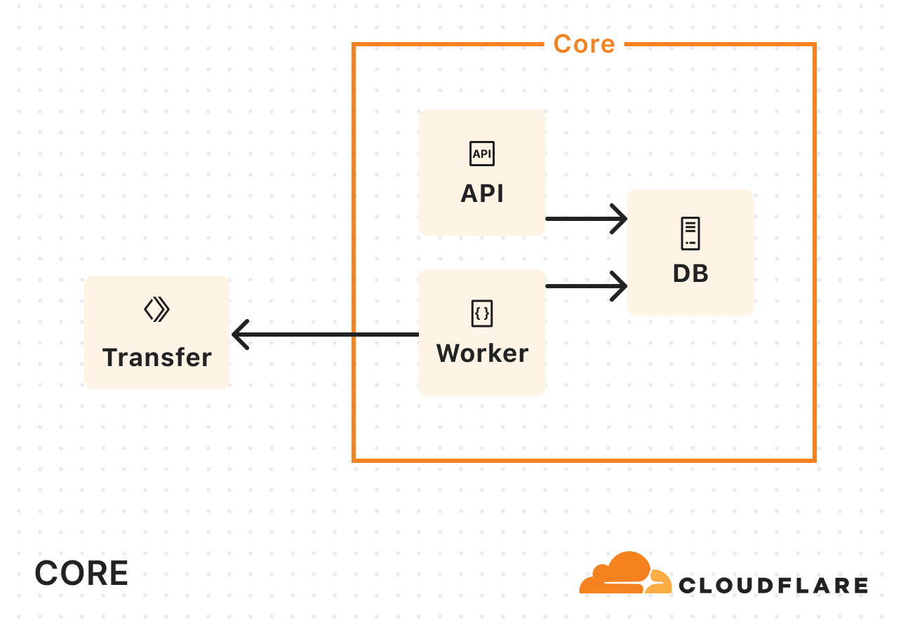
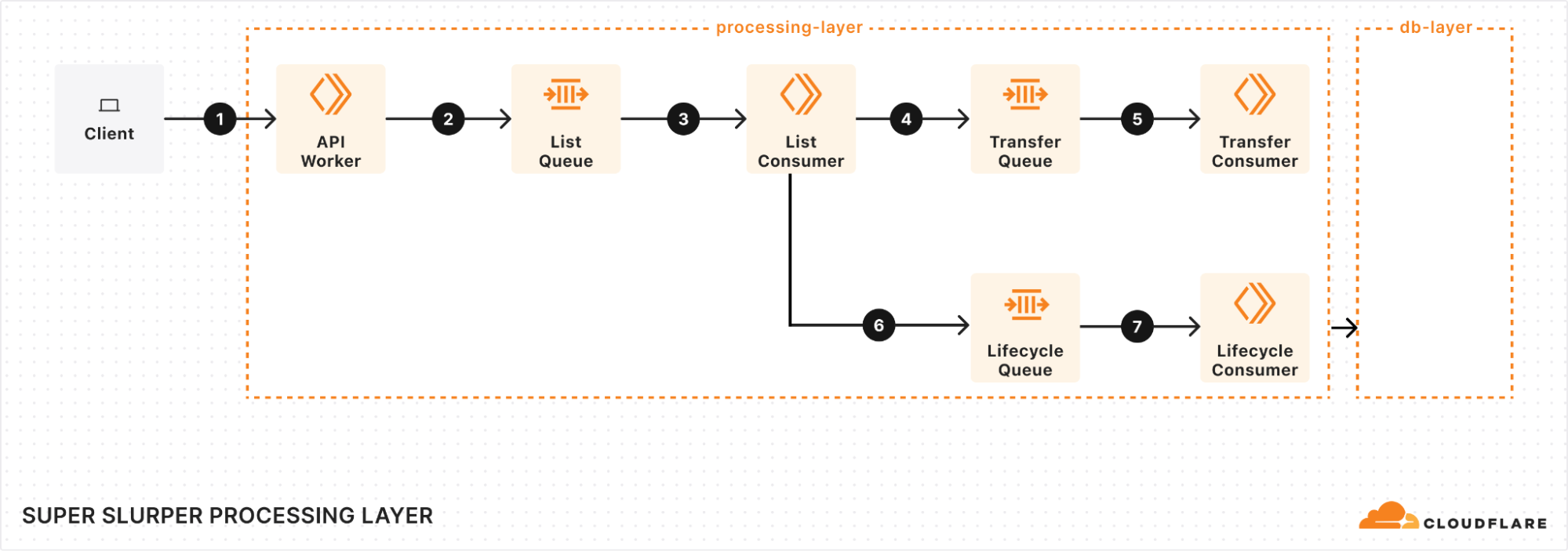
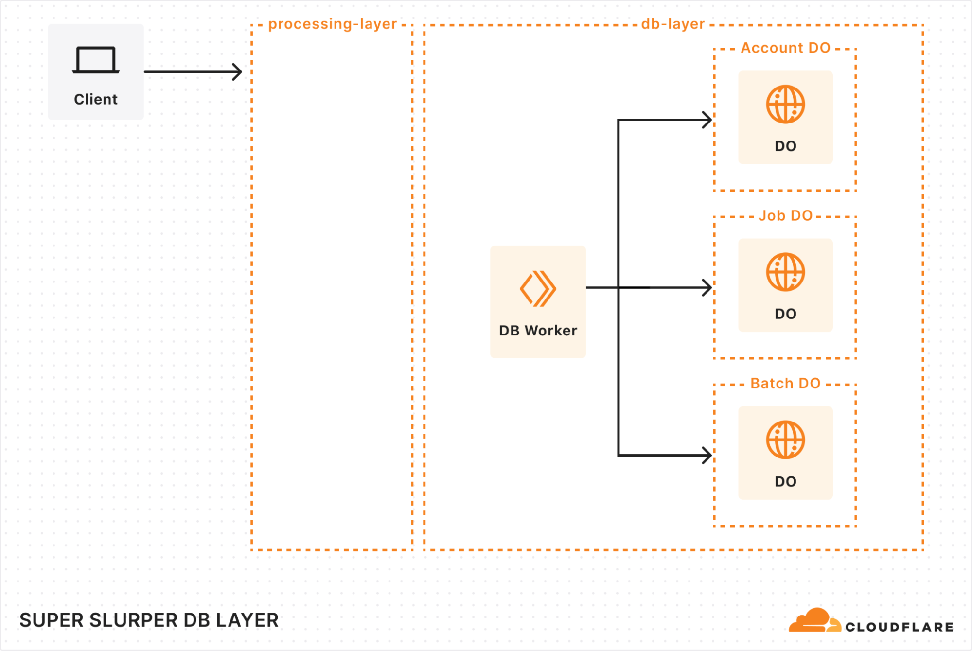
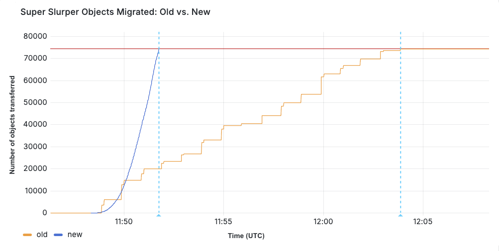


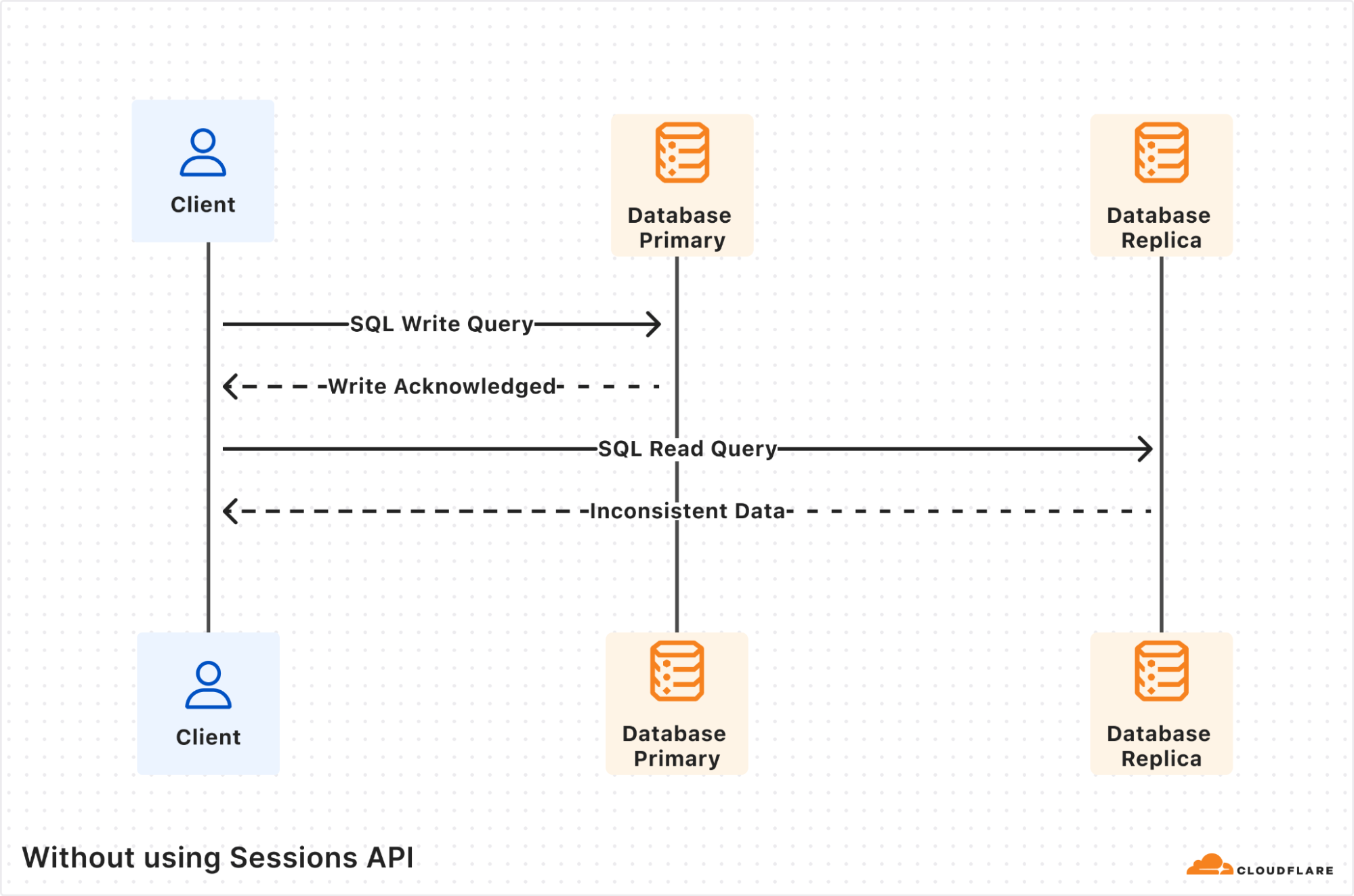
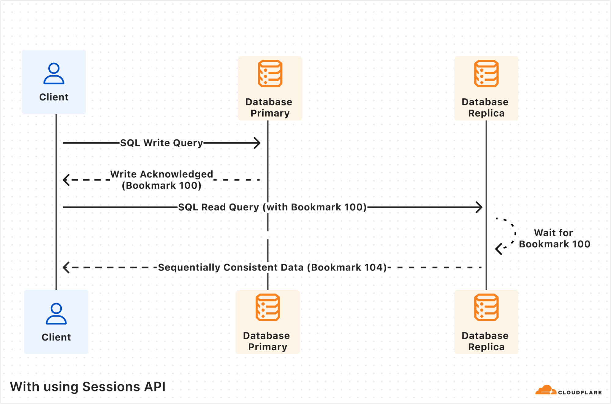
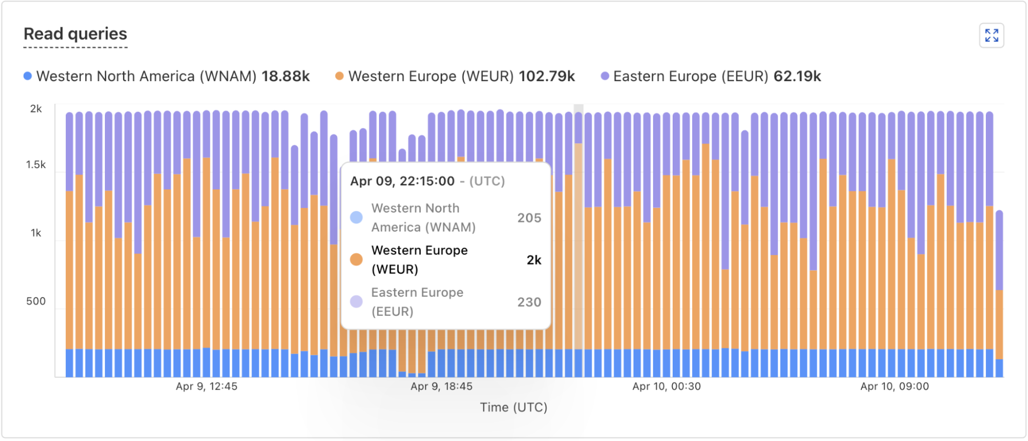
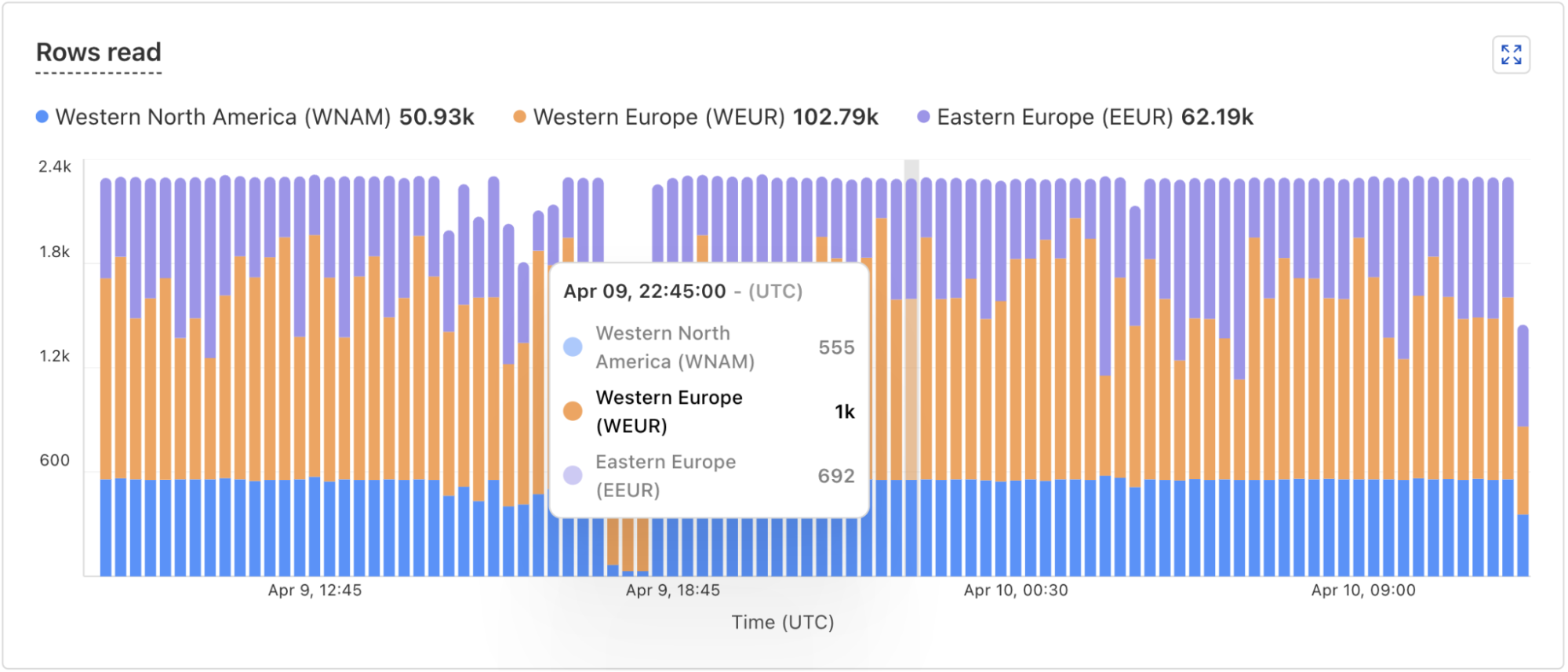
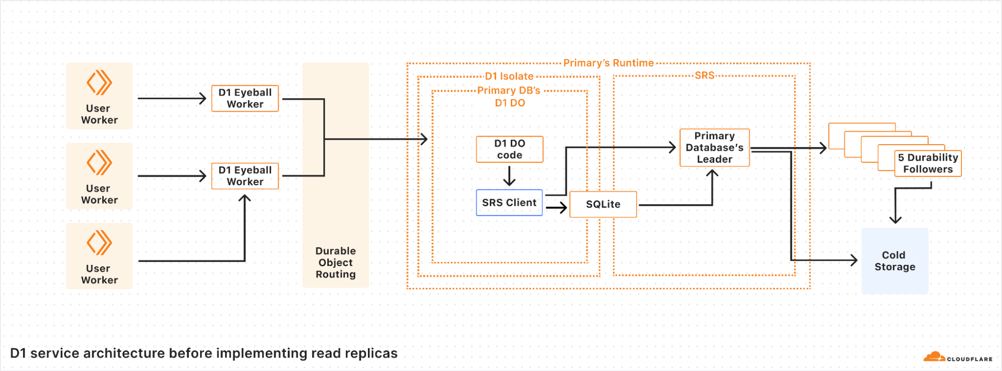
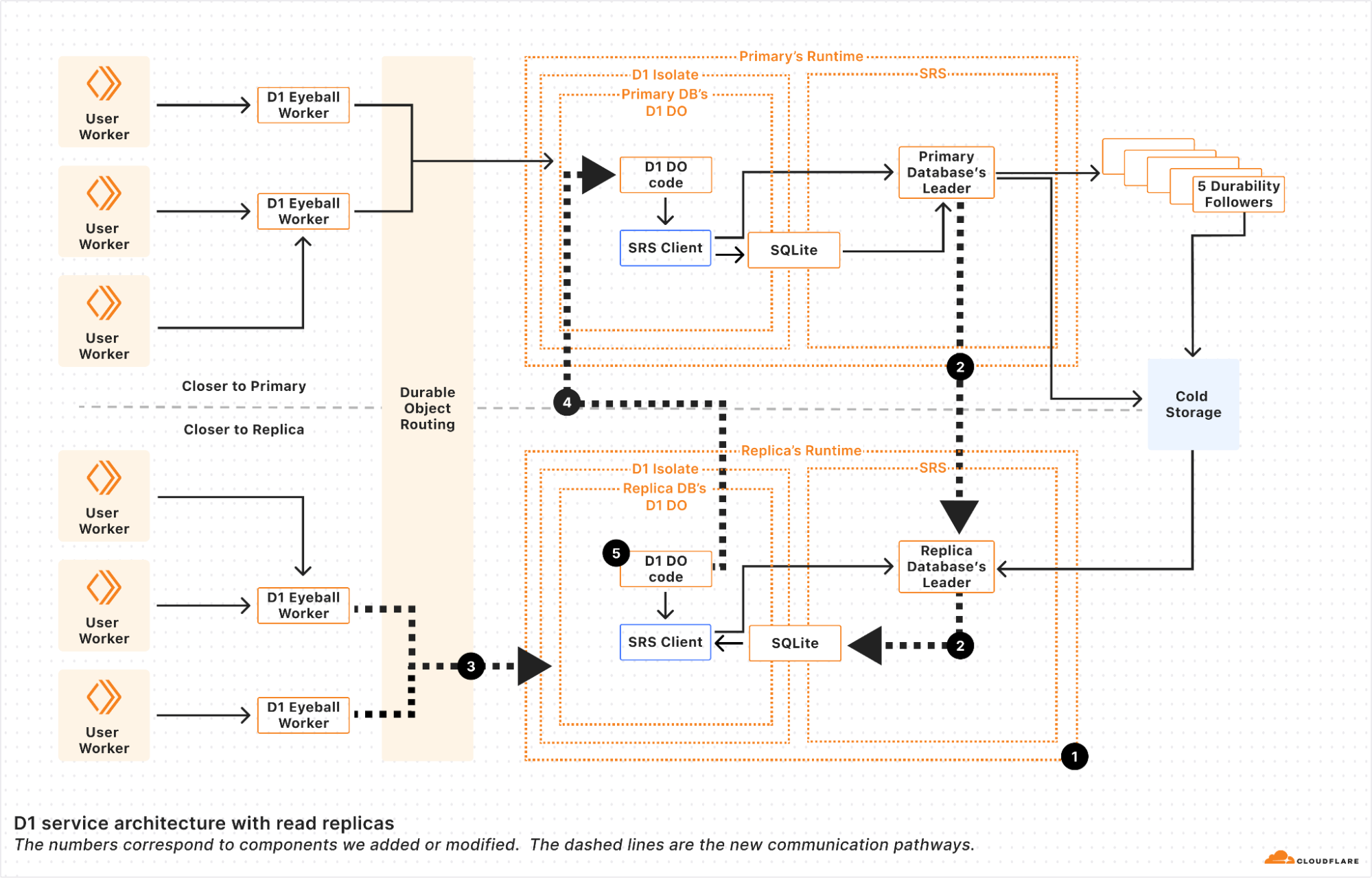
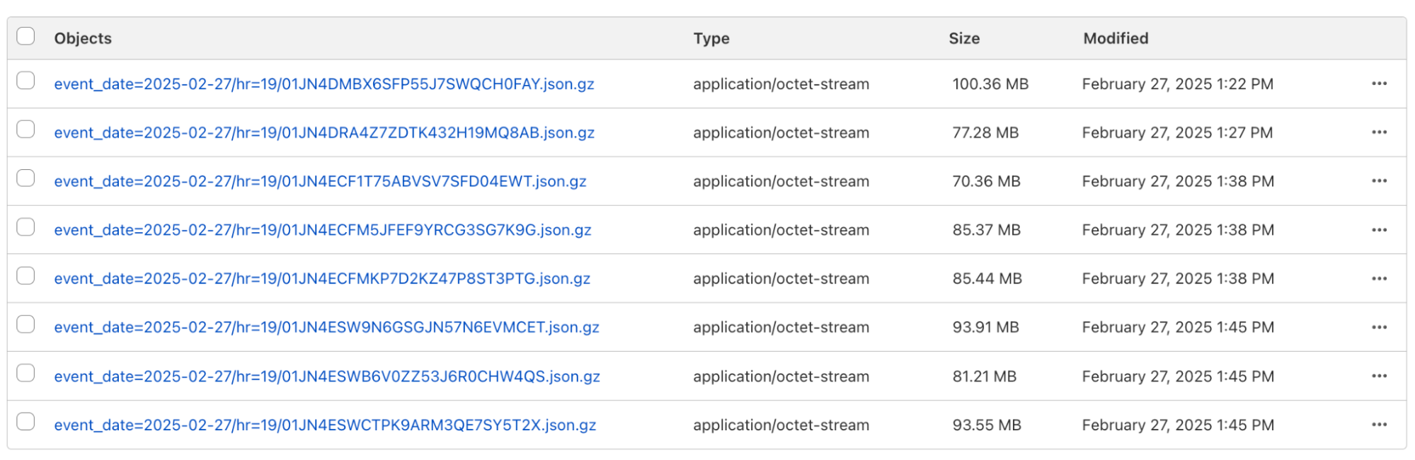
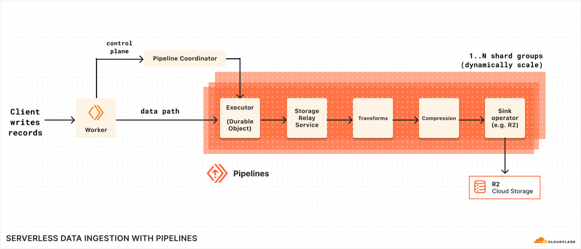










 Ramesh H Singh is a Senior Product Manager Technical (External Services) at AWS in Seattle, Washington, currently with the Amazon SageMaker team. He is passionate about building high-performance ML/AI and analytics products that enable enterprise customers to achieve their critical goals using cutting-edge technology. Connect with him on
  Pradeep Misra is a Principal Analytics Solutions Architect at AWS. He works across Amazon to architect and design modern distributed analytics and AI/ML platform solutions. He is passionate about solving customer challenges using data, analytics, and AI/ML. Outside of work, Pradeep likes exploring new places, trying new cuisines, and playing board games with his family. He also likes doing science experiments, building LEGOs and watching anime with his daughters.
 Rajat Mathur is a Software Development Manager at AWS, leading the Amazon DataZone and SageMaker Unified Studio engineering teams. His team designs, builds, and operates services which make it faster and easier for customers to catalog, discover, share, and govern data. With deep expertise in building distributed data systems at scale, Rajat plays a key role in advancing AWS’s data analytics and AI/ML capabilities.
 Jie Lan is a Software Engineer at AWS based in New York, where he works on the Amazon SageMaker team. He is passionate about developing cutting-edge solutions in the big data and AI space, helping customers leverage cloud technology to solve complex problems.


 Lorenzo Nicora works as Senior Streaming Solution Architect at AWS, helping customers across EMEA. He has been building cloud-centered, data-intensive systems for over 25 years, working across industries both through consultancies and product companies. He has used open-source technologies extensively and contributed to several projects, including Apache Flink, and is the maintainer of the Flink Prometheus connector.
 Francisco Morillo is a Senior Streaming Solutions Architect at AWS. Francisco works with AWS customers, helping them design real-time analytics architectures using AWS services, supporting Amazon MSK and Amazon Managed Service for Apache Flink. He is also a main contributor to the Flink Prometheus connector.


