Imagine that all of us—all of society—have landed on some alien planet and need to form a government: clean slate. We do not have any legacy systems from the United States or any other country. We do not have any special or unique interests to perturb our thinking. How would we govern ourselves? It is unlikely that we would use the systems we have today. Modern representative democracy was the best form of government that eighteenth-century technology could invent. The twenty-first century is very different: scientifically, technically, and philosophically. For example, eighteenth-century democracy was designed under the assumption that travel and communications were both hard.
Indeed, the very idea of representative government was a hack to get around technological limitations. Voting is easier now. Does it still make sense for all of us living in the same place to organize every few years and choose one of us to go to a single big room far away and make laws in our name? Representative districts are organized around geography because that was the only way that made sense two hundred-plus years ago. But we do not need to do it that way anymore. We could organize representation by age: one representative for the thirty-year-olds, another for the forty-year-olds, and so on. We could organize representation randomly: by birthday, perhaps. We can organize in any way we want. American citizens currently elect people to federal posts for terms ranging from two to six years. Would ten years be better for some posts? Would ten days be better for others? There are lots of possibilities. Maybe we can make more use of direct democracy by way of plebiscites. Certainly we do not want all of us, individually, to vote on every amendment to every bill, but what is the optimal balance between votes made in our name and ballot initiatives that we all vote on?
For the past three years, I have organized a series of annual two-day workshops to discuss these and other such questions.1 For each event, I brought together fifty people from around the world: political scientists, economists, law professors, experts in artificial intelligence, activists, government types, historians, science-fiction writers, and more. We did not come up with any answers to our questions—and I would have been surprised if we had—but several themes emerged from the event. Misinformation and propaganda was a theme, of course, and the inability to engage in rational policy discussions when we cannot agree on facts. The deleterious effects of optimizing a political system for economic outcomes was another theme. Given the ability to start over, would anyone design a system of government for the near-term financial interest of the wealthiest few? Another theme was capitalism and how it is or is not intertwined with democracy. While the modern market economy made a lot of sense in the industrial age, it is starting to fray in the information age. What comes after capitalism, and how will it affect the way we govern ourselves?
Many participants examined the effects of technology, especially artificial intelligence (AI). We looked at whether—and when—we might be comfortable ceding power to an AI system. Sometimes deciding is easy. I am happy for an AI system to figure out the optimal timing of traffic lights to ensure the smoothest flow of cars through my city. When will we be able to say the same thing about the setting of interest rates? Or taxation? How would we feel about an AI device in our pocket that voted in our name, thousands of times per day, based on preferences that it inferred from our actions? Or how would we feel if an AI system could determine optimal policy solutions that balanced every voter’s preferences: Would it still make sense to have a legislature and representatives? Possibly we should vote directly for ideas and goals instead, and then leave the details to the computers.
These conversations became more pointed in the second and third years of our workshop, after generative AI exploded onto the internet. Large language models are poised to write laws, enforce both laws and regulations, act as lawyers and judges, and plan political strategy. How this capacity will compare to human expertise and capability is still unclear, but the technology is changing quickly and dramatically. We will not have AI legislators anytime soon, but just as today we accept that all political speeches are professionally written by speechwriters, will we accept that future political speeches will all be written by AI devices? Will legislators accept AI-written legislation, especially when that legislation includes a level of detail that human-based legislation generally does not? And if so, how will that change affect the balance of power between the legislature and the administrative state? Most interestingly, what happens when the AI tools we use to both write and enforce laws start to suggest policy options that are beyond human understanding? Will we accept them, because they work? Or will we reject a system of governance where humans are only nominally in charge?
Scale was another theme of the workshops. The size of modern governments reflects the technology at the time of their founding. European countries and the early American states are a particular size because that was a governable size in the eighteenth and nineteenth centuries. Larger governments—those of the United States as a whole and of the European Union—reflect a world where travel and communications are easier. Today, though, the problems we have are either local, at the scale of cities and towns, or global. Do we really have need for a political unit the size of France or Virginia? Or is it a mixture of scales that we really need, one that moves effectively between the local and the global?
As to other forms of democracy, we discussed one from history and another made possible by today’s technology. Sortition is a system of choosing political officials randomly. We use it today when we pick juries, but both the ancient Greeks and some cities in Renaissance Italy used it to select major political officials. Today, several countries—largely in Europe—are using the process to decide policy on complex issues. We might randomly choose a few hundred people, representative of the population, to spend a few weeks being briefed by experts, debating the issues, and then deciding on environmental regulations, or a budget, or pretty much anything.
“Liquid democracy” is a way of doing away with elections altogether. The idea is that everyone has a vote and can assign it to anyone they choose. A representative collects the proxies assigned to him or her and can either vote directly on the issues or assign all the proxies to someone else. Perhaps proxies could be divided: this person for economic matters, another for health matters, a third for national defense, and so on. In the purer forms of this system, people might transfer their votes to someone else at any time. There would be no more election days: vote counts might change every day.
And then, there is the question of participation and, more generally, whose interests are taken into account. Early democracies were really not democracies at all; they limited participation by gender, race, and land ownership. These days, to achieve a more comprehensive electorate we could lower the voting age. But, of course, even children too young to vote have rights, and in some cases so do other species. Should future generations be given a “voice,” whatever that means? What about nonhumans, or whole ecosystems? Should everyone have the same volume and type of voice? Right now, in the United States, the very wealthy have much more influence than others do. Should we encode that superiority explicitly? Perhaps younger people should have a more powerful vote than everyone else. Or maybe older people should.
In the workshops, those questions led to others about the limits of democracy. All democracies have boundaries limiting what the majority can decide. We are not allowed to vote Common Knowledge out of existence, for example, but can generally regulate speech to some degree. We cannot vote, in an election, to jail someone, but we can craft laws that make a particular action illegal. We all have the right to certain things that cannot be taken away from us. In the community of our future, what should be our rights as individuals? What should be the rights of society, superseding those of individuals?
Personally, I was most interested, at each of the three workshops, in how political systems fail. As a security technologist, I study how complex systems are subverted—hacked, in my parlance—for the benefit of a few at the expense of the many. Think of tax loopholes, or tricks to avoid government regulation. These hacks are common today, and AI tools will make them easier to find—and even to design—in the future. I would want any government system to be resistant to trickery. Or, to put it another way: I want the interests of each individual to align with the interests of the group at every level. We have never had a system of government with this property, but—in a time of existential risks such as climate change—it is important that we develop one.
Would this new system of government even be called “democracy”? I truly do not know.
Such speculation is not practical, of course, but still is valuable. Our workshops did not produce final answers and were not intended to do so. Our discourse was filled with suggestions about how to patch our political system where it is fraying. People regularly debate changes to the US Electoral College, or the process of determining voting districts, or the setting of term limits. But those are incremental changes. It is difficult to find people who are thinking more radically: looking beyond the horizon—not at what is possible today but at what may be possible eventually. Thinking incrementally is critically important, but it is also myopic. It represents a hill-climbing strategy of continuous but quite limited improvements. We also need to think about discontinuous changes that we cannot easily get to from here; otherwise, we may be forever stuck at local maxima. And while true innovation in politics is a lot harder than innovation in technology, especially without a violent revolution forcing changes on us, it is something that we as a species are going to have to get good at, one way or another.
Our workshop will reconvene for a fourth meeting in December 2025.
Note
The First International Workshop on Reimagining Democracy (IWORD) was held December 7—8, 2022. The Second IWORD was held December 12—13, 2023. Both took place at the Harvard Kennedy School. The sponsors were the Ford Foundation, the Knight Foundation, and the Ash and Belfer Centers of the Kennedy School. See Schneier, “Recreating Democracy” and Schneier, “Second Interdisciplinary Workshop.”
At Grab, we operate a set of services that manage and provide counts of various items. While this may seem straightforward, the scale at which this feature operates—benefiting millions of Grab users daily—introduces complexity. This feature is divided into three microservices: one for “writing” counts, another for handling “read” requests, and a third serving as the backend for a portal used by data scientists and analysts to configure these counters.
This article focuses on the service responsible for handling “read” requests. This service is backed by Scylla storage and a Redis cache. It also connects to a MySQL RDS to retrieve “counter configurations” that are necessary for processing incoming requests. Written in Rust, the service serves tens of thousands of queries per second (QPS) during peak times, with each request typically being a “batch request” requiring multiple lookups (~10) on Scylla.
Recently, the service has encountered performance challenges, causing periodic spikes in Scylla QPS. These spikes occur throughout the day but are particularly evident during peak hours. To understand this better, we’ll first walk you through how this service operates, particularly how it serves incoming requests. We will then explain our proposed solution and the outcomes of our experiment.
Anatomy of a request
Each counter configuration stored in MySQL has a template that dictates the format of incoming queries. For example, this sample counter configuration is used to count the raindrops for a specific city:
An incoming request using this counter might look like this:
{
    "key": "rain_drops:city:111222",
    "fromTime": 1727215430, // 24 September 2024 22:03:50
    "toTime": 1727400000, // 27 September 2024 01:20:00
}
This request seeks the number of raindrops in our imaginary city with city ID: 111222, between 1727215430 (24 September 2024 22:03:50) and 1727400000 (27 September 2024 01:20:00).
Another service keeps track of raindrops by city and writes the minutely (truncated at 15 minutes), hourly, and daily counts to three different Scylla tables:
minutely_count_table
hourly_count_table
daily_count_table
The service processing the request rounds down the time to the nearest 15 minutes. As a result, the request is processed with the following time range:
Start time: 24 September 2024 22:00:00
End time: 27 September 2024 01:15:00
Let’s assume we have the following data in these three tables for “rain_drops:city:111222”. The datapoints used in the above example request are highlighted in bold.
minutely_count_table:
key
minutely_timestamp
count
rain_drops:city:111222
2024-09-24T22:00:00Z
3
rain_drops:city:111222
2024-09-24T22:15:00Z
2
rain_drops:city:111222
2024-09-24T22:30:00Z
4
rain_drops:city:111222
2024-09-24T22:45:00Z
1
…
…
…
rain_drops:city:111222
2024-09-27T01:00:00Z
2
rain_drops:city:111222
2024-09-27T01:15:00Z
3
hourly_count_table:
key
hourly_timestamp
count
rain_drops:city:111222
2024-09-24T22:00:00Z
18
rain_drops:city:111222
2024-09-24T23:00:00Z
22
rain_drops:city:111222
2024-09-25T00:00:00Z
15
…
…
…
rain_drops:city:111222
2024-09-27T00:00:00Z
11
rain_drops:city:111222
2024-09-27T01:00:00Z
9
daily_count_table:
key
daily_timestamp
count
rain_drops:city:111222
2024-09-24T00:00:00Z
214
rain_drops:city:111222
2024-09-25T00:00:00Z
189
rain_drops:city:111222
2024-09-26T00:00:00Z
245
rain_drops:city:111222
2024-09-27T00:00:00Z
78
Now, let’s see how the service calculates the total count for the incoming request with “rain_drops:city:111222” based on the provided data:
Time range:
From: 24 September 2024 22:03:50
To: 27 September 2024 01:20:00
For the full days within the range, specifically 25th and 26th September, we can use data from the daily_count_table. However, for the start (24th September) and end (27th September) date of the range, we cannot use data from the daily_count_table as the range only includes portions of these dates. Instead, we will use a combination of data from the hourly_count_table and minutely_count_table to accurately capture the counts for these days.
Query the daily_count_table:
Sum (full day: 25 and 26th Sep): 189 + 245 = 434
Query the hourly_count_table:
For 24th September (from 22:00:00 to 23:59:59):
Hourly count: 18 + 22 = 40
For 27th September (from 00:00:00 to 01:00:00):
Hourly count: 11
Query the minutely_count_table:
For 27th September (from 01:00:00 to 01:15:00):
Minutely count: 2
Total count:
Total = Daily count (25th and 26th) + Hourly count (24th) + Hourly count (27th) + Minutely count (27th)
= 434 + 40 + 11 + 2
= 487
Figure 1: The example request for “rain_drops:city:111222” is handled using data from three different Scylla tables.
As shown in the calculation, when the service receives the request, it comes up with the total count of raindrops by querying three Scylla tables and summing them up using some specific rules within the service itself.
Querying the cache
In the previous section, we explained how Scylla handles a query. If we cached the response for the same request earlier, retrieval from the cache follows a simpler logic. For instance, for the example request, the total count is stored using the floored start and end times (rounded to the nearest 15-minute window within an hour), which was used for the Scylla query instead of the original time in the request. The cache key-value pair would look like this:
Timestamps 1727215200 and 1727399700 represent the adjusted start and end times of 24 September 2024 22:00:00 and 27 September 2024 01:15:00, respectively. It has a Time-To-Live (TTL) of 5 minutes. During this TTL window, any request for the key “rain_drops:city:111222” having the same start and end times (after rounding to the nearest 15 minutes) will be read from the cache instead of querying Scylla.
For example, for the following three start times, although they are different, after flooring the request to the nearest 15 minutes, the start time becomes 24 September 2024 22:00:00 for all of them, which is the same start time as the one in the cache.
24 September 2024 22:01:00
24 September 2024 22:02:00
24 September 2024 22:06:00
In day-to-day operations, this caching setup allows roughly half of our total production requests to be served by the Redis cache.
Figure 2. The graph visualises the relative quantity of cache hits vs Scylla-bound requests.
Problem statement
The setup consisting of Scylla and Redis cache works well. Particularly because Scylla-bound queries need to look up 1-3 tables (minutely, hourly, daily, depending on the time range) and perform the summation as explained earlier, whereas a single cache lookup gets the final value for the same query. However, as our cache key pattern follows the 15-minute truncation strategy, along with a 5-minute cache TTL, it leads to an interesting phenomenon – our cache hits plummet and Scylla QPS spikes at the end of every 15 minutes.
Figure 3. Graph showing 15-minute spikes in Scylla-bound requests accompanied by a decline in cache hit rates.
This occurs primarily due to the fact that almost all requests to our service are for recent data. Due to this, at the end of every 15-minute block within an hour (i.e., 00, 15, 30, 45), most of the requests require creating new cache keys for the latest 15-minute block. At this point in time, there may be many unexpired (i.e., have not reached 5 min TTL) cache keys from the previous 15-minutes block, but they become less relevant as most requests are asking for recent data.
The table in Figure 4 shows example data for configurations “rain_drops:city:111222” and “bird_sighting:city:333444”. For these two configurations, new cache keys are created due to TTL expiry at random times. However, at the end of the 15-minute block, which, in this case is at the end of 22:00-22:15 block, both configurations need new cache keys for the new 15-minute time block that has just started (i.e., start of 22:15-22:30), even though some of their cache keys from the previous 15-minute block are still valid. This requirement of creating new cache keys for most of the requests at the end of a 15-minute block causes spikes in Scylla QPS and a sharp decline in cache hits.
One question that arises is – “Why don’t we see a spike every 5 minutes for cache key TTL expiry?” This is because, within the 15 minutes block, new cache keys are continuously created when a key reaches TTL and a new request for that is received. Since this happens all the time as shown in Figure 4, we do not see a sharp spike. In other words, although Scylla does receive more queries due to cache TTL expiry, it does not lead to a spike in Scylla queries or a sharp drop in cache hits. This is because the cache keys are always being created and invalidated due to TTL expiry instead of following a fixed 5-minute block similar to the 15-minute block we use for our truncation strategy.
Figure 4. This table visualises scenarios when new cache keys are required due to TTL expiry vs due to 15-minute truncation strategy.
These Scylla QPS spikes at the end of every 15-minute block lead to a highly imbalanced Scylla QPS. This often causes high latency in our service during the 15-minute blocks that fall within the peak traffic hours. This further causes more requests to time out, eventually increasing the number of failed requests.
Proposed solution
We propose mitigating this issue by completely removing the Redis-backed caching mechanism from the service. Our observations indicate that the Scylla spikes at the end of 15-minute blocks occur due to cache hit misses. Therefore, removing the caching should eliminate the spikes and provide for a more balanced load.
We acknowledge that this may seem counterintuitive from an overall performance standpoint as removing caching means all queries will be Scylla-bound, potentially impacting the overall performance since caching usually speeds up processes. In addition, caching also comes with an advantage where for cache hits, the service does not need to do the summation on Scylla results from minutely, hourly, and the daily table. Despite these shortcomings, we hypothesise that removing caching should not have an adverse impact on the overall performance. This is based on the fact the Scylla has its own sophisticated caching mechanism. However, our existing setup uses Redis for caching, underutilising Scylla’s cache as the most subsequent queries hit the Redis cache instead.
In summary, we propose eliminating the Redis caching component from our current architecture. This change is expected to resolve the Scylla query spikes observed at the end of every 15-minute block. By relying on Scylla’s native caching mechanism, we anticipate maintaining the service’s overall performance more effectively. The removal of Redis is counterbalanced by the optimised utilisation of Scylla’s built-in caching capabilities.
Experiment
Procedure
The experiment was done on an important live service serving thousands of QPS. To avoid disruptions, we followed a gradual approach. We first turned off caching for a few configurations. If there were no adverse impacts observed, we incrementally disabled cache for more configurations. We controlled the rollout increment by using a mathematical operator on the configuration IDs. This approach is simple and allows us to deterministically disable the cache for specific configurations across all requests, as opposed to using a percentage rollout which randomly disables the cache for different configurations across different requests. This is also due to the fact that the number of configurations is relatively steady and small (less than a thousand). Since these configurations are already fully cached in the service memory from RDS, there will be no performance impact of having a condition that operates on these configurations.
To make sense of the graphs and metrics reported in this section, it is important to understand the traffic pattern of this service. The service usually sees two peaks every day: noon and another around 6-7 PM. On a weekly basis, we usually see the highest traffic on Friday, with the busiest period being from 6-8 PM.
In addition, the timeline of when and how we made various changes to our setup is important to accurately interpret our results.
Experiment timeline: Nov 5 – Nov 13, 2024:
Redis cache disabled for ~5% of the counter configurations – Nov 5, 2024, 10.26 AM (Canary started: 10.00 AM)
Redis cache disabled for ~25% of the counter configurations – Nov 5, 2024, 12.44 PM (Canary started: 12.20 PM)
Redis cache disabled for ~35% of the counter configurations – Nov 6, 2024, 10.50 AM (Canary started: 10.21 AM)
Redis cache disabled for ~75% of the counter configurations – Nov 7, 2024, 10.53 AM (Canary started: 10.26 AM)
Experimenting with running a major compaction job during the day time: Tue, Nov 12, 2024, between 2-5 PM (on all nodes)
Day time scheduled major compaction job starts from: Tue, Nov 13, 2024, between 2-5 PM (on all nodes)
Redis cache disabled for 100% of the counter configs – Wed, 13 Nov 2024, 10:56 AM (Canary started: 10:32 AM)
Unless otherwise specified, the graphs and metrics we report in this article uses this fixed time window: Oct 31 (Thu) 12.00 AM – Nov 15 (Friday) 11.59 PM SGT. This time window covers the entire experiment period with some buffer to observe the experiment’s impact.
Observations
As we progressively disabled read from external Redis cache over the span of 8 days (Nov 5 – Nov 13), we made interesting observations and experimented with some Scylla configuration changes on our end. We describe them in the following sections.
Scylla hit vs. cache hit
As we progressively disabled Redis cache for most of the counters, one obvious impact was the gradual increase in Scylla-bound QPS and similar decrease in Redis-cache hit. When Redis-cache was enabled for 100% of the configurations, 50% of the requests were bound for Scylla and the other 50% were for Redis. At the end of the experiment, after fully disabling Redis cache, 100% of the requests were Scylla-bound.
Figure 5. Gradual increase in Scylla QPS and simultaneous decrease in Redis cache hit.
15-minutes and hourly spikes
We noticed that the 15-minute spikes in Scylla QPS as well as the associated latency slowly became less prominent and eventually disappeared from the graph after we completely disabled the Redis cache. However, we noticed that the hourly spike still remained. This is attributed to the higher QPS from the clients calling this service at the turn of every hour. As a result, limited optimisation can be done to reduce the hourly spike on this service’s end.
Figure 6. The 15-minute spikes in Scylla QPS disappeared after the external Redis cache was fully disabled. This graph uses a smaller time window to show the earlier spikes. It also shows the persistence of hourly spikes after the experiment which is attributed to the clients of this service sending more requests at the start of every hour.
Figure 7. The graph shows that the 15-minute spikes in Scylla’s latency disappeared after the external Redis cache was fully disabled. This graph uses a smaller time window to show the earlier spikes. It also shows the persistence of hourly spikes in latency after the experiment which is attributed to the clients of this service sending more requests at the start of every hour.
Service latency and additional Scylla compaction job
When we disabled Redis cache for about 75% of the counters configurations on Nov 7 (which accounts for about 85% of the overall QPS), we noticed an increase in the overall average service latency, from between 6-8 ms to 7-12 ms (P99 went from ~30-50ms to ~30-70ms). This caused a spike in open circuit breaker (CB) events on Hystrix. At this point, before disabling cache for more counters, on Nov 12, we experimented with running an additional major compaction job on Scylla between 2-5 PM on all our Scylla nodes, progressively on each availability zone (AZ). It is noteworthy that we already have a scheduled major compaction job that runs around 3 AM every day. The outcome of this experiment was quite positive. It brought back the average and P99 latency almost to the prior level when we had Redis cache enabled for 100% of the counters. This also had a similar effect on the Hystrix CB open events. Based on this observation, we made this additional day time major compaction job as a daily scheduled job. We disabled Redis cache for 100% of the counters the next day (Nov 13). This expectedly increased the Scylla QPS, with no noticeable adverse effect on the service latency or Hystrix CB open events.
Figure 8. This graph shows how the average latency changed as a result of the experiment. The higher spikes correspond to the time when Redis cache was being progressively disabled before introducing the day time Scylla compaction job. The spikes lessened after the compaction job was introduced on Nov 12 (Note: Friday spike was due to higher traffic in general).
Figure 9. This graph shows how the P99 latency changed as a result of the experiment. The higher spikes correspond to the time when Redis cache was being progressively disabled before introducing the day time Scylla compaction job. The spikes lessened after the compaction job was introduced on Nov 12 (Note: Friday spike was due to higher traffic in general).
Scylla’s own cache
One of our hypotheses was that we were not using Scylla cache due to our system’s design, along with all the service specific characteristics discussed earlier. Our experimental results show that this is indeed the case. We observed a significant increase in Scylla reads with Scylla’s own cache hits, while Scylla reads with Scylla’s own cache misses remained about the same despite our Scylla cluster receiving double the traffic. Percentage-wise, before disabling the external Redis cache, Scylla hit its own cache for ~30% of the total reads, and after we have completely disabled the external Redis cache, Scylla hit its cache for about 70% of the reads. We believe that this largely contributes to the overall performance of the service despite fully decommissioning the expensive Redis cache component from our system architecture.
Figure 10. Significant increase in Scylla reads after disable Redis cache.
Figure 11. No change in Scylla cache miss despite the doubling of Scylla traffic.
Scylla CPU and memory usage
Contrary to our assumption, although the Scylla QPS doubled due to the change done as part of this experiment, there was marginal increase in Scylla CPU usage (from ~50% to ~52% at peak). In terms of memory, Scylla log-structured allocator (LSA) memory usage remains consistent. For Non-LSA memory, the maximum utilisation did not increase. However, we noticed two daily spikes instead of one existed before the experiment. The second spike results from the newly added daily major compaction job. Notably,the overall non-LSA peak has slightly decreased after the introduction of the new compaction job.
Figure 12. Relatively steady Scylla CPU utilisation.
Figure 13. Non-LSA memory usage spikes twice a day after the experiment. The new spike corresponds to the newly added day time compaction job.
Conclusion
In summary, we were able to maintain the same service performance while removing an expensive Redis cache component from our system architecture, which accounted for about 25% of the overall service cost. This has been made possible primarily by significant increase in the utilisation of Scylla’s own cache and adding a daily major compaction job on all our Scylla nodes.
In the future, we plan to further experiment with different Scylla configurations for potential performance gain, specifically to improve the latency.
Join us
Grab is a leading superapp in Southeast Asia, operating across the deliveries, mobility and digital financial services sectors. Serving over 800 cities in eight Southeast Asian countries, Grab enables millions of people everyday to order food or groceries, send packages, hail a ride or taxi, pay for online purchases or access services such as lending and insurance, all through a single app. Grab was founded in 2012 with the mission to drive Southeast Asia forward by creating economic empowerment for everyone. Grab strives to serve a triple bottom line – we aim to simultaneously deliver financial performance for our shareholders and have a positive social impact, which includes economic empowerment for millions of people in the region, while mitigating our environmental footprint.
Powered by technology and driven by heart, our mission is to drive Southeast Asia forward by creating economic empowerment for everyone. If this mission speaks to you, join our team today!
At Grab, we operate a set of services that manage and provide counts of various items. While this may seem straightforward, the scale at which this feature operates—benefiting millions of Grab users daily—introduces complexity. This feature is divided into three microservices: one for “writing” counts, another for handling “read” requests, and a third serving as the backend for a portal used by data scientists and analysts to configure these counters.
This article focuses on the service responsible for handling “read” requests. This service is backed by Scylla storage and a Redis cache. It also connects to a MySQL RDS to retrieve “counter configurations” that are necessary for processing incoming requests. Written in Rust, the service serves tens of thousands of queries per second (QPS) during peak times, with each request typically being a “batch request” requiring multiple lookups (~10) on Scylla.
Recently, the service has encountered performance challenges, causing periodic spikes in Scylla QPS. These spikes occur throughout the day but are particularly evident during peak hours. To understand this better, we’ll first walk you through how this service operates, particularly how it serves incoming requests. We will then explain our proposed solution and the outcomes of our experiment.
Anatomy of a request
Each counter configuration stored in MySQL has a template that dictates the format of incoming queries. For example, this sample counter configuration is used to count the raindrops for a specific city:
An incoming request using this counter might look like this:
{
    "key": "rain_drops:city:111222",
    "fromTime": 1727215430, // 24 September 2024 22:03:50
    "toTime": 1727400000, // 27 September 2024 01:20:00
}
This request seeks the number of raindrops in our imaginary city with city ID: 111222, between 1727215430 (24 September 2024 22:03:50) and 1727400000 (27 September 2024 01:20:00).
Another service keeps track of raindrops by city and writes the minutely (truncated at 15 minutes), hourly, and daily counts to three different Scylla tables:
minutely_count_table
hourly_count_table
daily_count_table
The service processing the request rounds down the time to the nearest 15 minutes. As a result, the request is processed with the following time range:
Start time: 24 September 2024 22:00:00
End time: 27 September 2024 01:15:00
Let’s assume we have the following data in these three tables for “rain_drops:city:111222”. The datapoints used in the above example request are highlighted in bold.
minutely_count_table:
key
minutely_timestamp
count
rain_drops:city:111222
2024-09-24T22:00:00Z
3
rain_drops:city:111222
2024-09-24T22:15:00Z
2
rain_drops:city:111222
2024-09-24T22:30:00Z
4
rain_drops:city:111222
2024-09-24T22:45:00Z
1
…
…
…
rain_drops:city:111222
2024-09-27T01:00:00Z
2
rain_drops:city:111222
2024-09-27T01:15:00Z
3
hourly_count_table:
key
hourly_timestamp
count
rain_drops:city:111222
2024-09-24T22:00:00Z
18
rain_drops:city:111222
2024-09-24T23:00:00Z
22
rain_drops:city:111222
2024-09-25T00:00:00Z
15
…
…
…
rain_drops:city:111222
2024-09-27T00:00:00Z
11
rain_drops:city:111222
2024-09-27T01:00:00Z
9
daily_count_table:
key
daily_timestamp
count
rain_drops:city:111222
2024-09-24T00:00:00Z
214
rain_drops:city:111222
2024-09-25T00:00:00Z
189
rain_drops:city:111222
2024-09-26T00:00:00Z
245
rain_drops:city:111222
2024-09-27T00:00:00Z
78
Now, let’s see how the service calculates the total count for the incoming request with “rain_drops:city:111222” based on the provided data:
Time range:
From: 24 September 2024 22:03:50
To: 27 September 2024 01:20:00
For the full days within the range, specifically 25th and 26th September, we can use data from the daily_count_table. However, for the start (24th September) and end (27th September) date of the range, we cannot use data from the daily_count_table as the range only includes portions of these dates. Instead, we will use a combination of data from the hourly_count_table and minutely_count_table to accurately capture the counts for these days.
Query the daily_count_table:
Sum (full day: 25 and 26th Sep): 189 + 245 = 434
Query the hourly_count_table:
For 24th September (from 22:00:00 to 23:59:59):
Hourly count: 18 + 22 = 40
For 27th September (from 00:00:00 to 01:00:00):
Hourly count: 11
Query the minutely_count_table:
For 27th September (from 01:00:00 to 01:15:00):
Minutely count: 2
Total count:
Total = Daily count (25th and 26th) + Hourly count (24th) + Hourly count (27th) + Minutely count (27th)
= 434 + 40 + 11 + 2
= 487
Figure 1: The example request for “rain_drops:city:111222” is handled using data from three different Scylla tables.
As shown in the calculation, when the service receives the request, it comes up with the total count of raindrops by querying three Scylla tables and summing them up using some specific rules within the service itself.
Querying the cache
In the previous section, we explained how Scylla handles a query. If we cached the response for the same request earlier, retrieval from the cache follows a simpler logic. For instance, for the example request, the total count is stored using the floored start and end times (rounded to the nearest 15-minute window within an hour), which was used for the Scylla query instead of the original time in the request. The cache key-value pair would look like this:
Timestamps 1727215200 and 1727399700 represent the adjusted start and end times of 24 September 2024 22:00:00 and 27 September 2024 01:15:00, respectively. It has a Time-To-Live (TTL) of 5 minutes. During this TTL window, any request for the key “rain_drops:city:111222” having the same start and end times (after rounding to the nearest 15 minutes) will be read from the cache instead of querying Scylla.
For example, for the following three start times, although they are different, after flooring the request to the nearest 15 minutes, the start time becomes 24 September 2024 22:00:00 for all of them, which is the same start time as the one in the cache.
24 September 2024 22:01:00
24 September 2024 22:02:00
24 September 2024 22:06:00
In day-to-day operations, this caching setup allows roughly half of our total production requests to be served by the Redis cache.
Figure 2. The graph visualises the relative quantity of cache hits vs Scylla-bound requests.
Problem statement
The setup consisting of Scylla and Redis cache works well. Particularly because Scylla-bound queries need to look up 1-3 tables (minutely, hourly, daily, depending on the time range) and perform the summation as explained earlier, whereas a single cache lookup gets the final value for the same query. However, as our cache key pattern follows the 15-minute truncation strategy, along with a 5-minute cache TTL, it leads to an interesting phenomenon – our cache hits plummet and Scylla QPS spikes at the end of every 15 minutes.
Figure 3. Graph showing 15-minute spikes in Scylla-bound requests accompanied by a decline in cache hit rates.
This occurs primarily due to the fact that almost all requests to our service are for recent data. Due to this, at the end of every 15-minute block within an hour (i.e., 00, 15, 30, 45), most of the requests require creating new cache keys for the latest 15-minute block. At this point in time, there may be many unexpired (i.e., have not reached 5 min TTL) cache keys from the previous 15-minutes block, but they become less relevant as most requests are asking for recent data.
The table in Figure 4 shows example data for configurations “rain_drops:city:111222” and “bird_sighting:city:333444”. For these two configurations, new cache keys are created due to TTL expiry at random times. However, at the end of the 15-minute block, which, in this case is at the end of 22:00-22:15 block, both configurations need new cache keys for the new 15-minute time block that has just started (i.e., start of 22:15-22:30), even though some of their cache keys from the previous 15-minute block are still valid. This requirement of creating new cache keys for most of the requests at the end of a 15-minute block causes spikes in Scylla QPS and a sharp decline in cache hits.
One question that arises is – “Why don’t we see a spike every 5 minutes for cache key TTL expiry?” This is because, within the 15 minutes block, new cache keys are continuously created when a key reaches TTL and a new request for that is received. Since this happens all the time as shown in Figure 4, we do not see a sharp spike. In other words, although Scylla does receive more queries due to cache TTL expiry, it does not lead to a spike in Scylla queries or a sharp drop in cache hits. This is because the cache keys are always being created and invalidated due to TTL expiry instead of following a fixed 5-minute block similar to the 15-minute block we use for our truncation strategy.
Figure 4. This table visualises scenarios when new cache keys are required due to TTL expiry vs due to 15-minute truncation strategy.
These Scylla QPS spikes at the end of every 15-minute block lead to a highly imbalanced Scylla QPS. This often causes high latency in our service during the 15-minute blocks that fall within the peak traffic hours. This further causes more requests to time out, eventually increasing the number of failed requests.
Proposed solution
We propose mitigating this issue by completely removing the Redis-backed caching mechanism from the service. Our observations indicate that the Scylla spikes at the end of 15-minute blocks occur due to cache hit misses. Therefore, removing the caching should eliminate the spikes and provide for a more balanced load.
We acknowledge that this may seem counterintuitive from an overall performance standpoint as removing caching means all queries will be Scylla-bound, potentially impacting the overall performance since caching usually speeds up processes. In addition, caching also comes with an advantage where for cache hits, the service does not need to do the summation on Scylla results from minutely, hourly, and the daily table. Despite these shortcomings, we hypothesise that removing caching should not have an adverse impact on the overall performance. This is based on the fact the Scylla has its own sophisticated caching mechanism. However, our existing setup uses Redis for caching, underutilising Scylla’s cache as the most subsequent queries hit the Redis cache instead.
In summary, we propose eliminating the Redis caching component from our current architecture. This change is expected to resolve the Scylla query spikes observed at the end of every 15-minute block. By relying on Scylla’s native caching mechanism, we anticipate maintaining the service’s overall performance more effectively. The removal of Redis is counterbalanced by the optimised utilisation of Scylla’s built-in caching capabilities.
Experiment
Procedure
The experiment was done on an important live service serving thousands of QPS. To avoid disruptions, we followed a gradual approach. We first turned off caching for a few configurations. If there were no adverse impacts observed, we incrementally disabled cache for more configurations. We controlled the rollout increment by using a mathematical operator on the configuration IDs. This approach is simple and allows us to deterministically disable the cache for specific configurations across all requests, as opposed to using a percentage rollout which randomly disables the cache for different configurations across different requests. This is also due to the fact that the number of configurations is relatively steady and small (less than a thousand). Since these configurations are already fully cached in the service memory from RDS, there will be no performance impact of having a condition that operates on these configurations.
To make sense of the graphs and metrics reported in this section, it is important to understand the traffic pattern of this service. The service usually sees two peaks every day: noon and another around 6-7 PM. On a weekly basis, we usually see the highest traffic on Friday, with the busiest period being from 6-8 PM.
In addition, the timeline of when and how we made various changes to our setup is important to accurately interpret our results.
Experiment timeline: Nov 5 – Nov 13, 2024:
Redis cache disabled for ~5% of the counter configurations – Nov 5, 2024, 10.26 AM (Canary started: 10.00 AM)
Redis cache disabled for ~25% of the counter configurations – Nov 5, 2024, 12.44 PM (Canary started: 12.20 PM)
Redis cache disabled for ~35% of the counter configurations – Nov 6, 2024, 10.50 AM (Canary started: 10.21 AM)
Redis cache disabled for ~75% of the counter configurations – Nov 7, 2024, 10.53 AM (Canary started: 10.26 AM)
Experimenting with running a major compaction job during the day time: Tue, Nov 12, 2024, between 2-5 PM (on all nodes)
Day time scheduled major compaction job starts from: Tue, Nov 13, 2024, between 2-5 PM (on all nodes)
Redis cache disabled for 100% of the counter configs – Wed, 13 Nov 2024, 10:56 AM (Canary started: 10:32 AM)
Unless otherwise specified, the graphs and metrics we report in this article uses this fixed time window: Oct 31 (Thu) 12.00 AM – Nov 15 (Friday) 11.59 PM SGT. This time window covers the entire experiment period with some buffer to observe the experiment’s impact.
Observations
As we progressively disabled read from external Redis cache over the span of 8 days (Nov 5 – Nov 13), we made interesting observations and experimented with some Scylla configuration changes on our end. We describe them in the following sections.
Scylla hit vs. cache hit
As we progressively disabled Redis cache for most of the counters, one obvious impact was the gradual increase in Scylla-bound QPS and similar decrease in Redis-cache hit. When Redis-cache was enabled for 100% of the configurations, 50% of the requests were bound for Scylla and the other 50% were for Redis. At the end of the experiment, after fully disabling Redis cache, 100% of the requests were Scylla-bound.
Figure 5. Gradual increase in Scylla QPS and simultaneous decrease in Redis cache hit.
15-minutes and hourly spikes
We noticed that the 15-minute spikes in Scylla QPS as well as the associated latency slowly became less prominent and eventually disappeared from the graph after we completely disabled the Redis cache. However, we noticed that the hourly spike still remained. This is attributed to the higher QPS from the clients calling this service at the turn of every hour. As a result, limited optimisation can be done to reduce the hourly spike on this service’s end.
Figure 6. The 15-minute spikes in Scylla QPS disappeared after the external Redis cache was fully disabled. This graph uses a smaller time window to show the earlier spikes. It also shows the persistence of hourly spikes after the experiment which is attributed to the clients of this service sending more requests at the start of every hour.
Figure 7. The graph shows that the 15-minute spikes in Scylla’s latency disappeared after the external Redis cache was fully disabled. This graph uses a smaller time window to show the earlier spikes. It also shows the persistence of hourly spikes in latency after the experiment which is attributed to the clients of this service sending more requests at the start of every hour.
Service latency and additional Scylla compaction job
When we disabled Redis cache for about 75% of the counters configurations on Nov 7 (which accounts for about 85% of the overall QPS), we noticed an increase in the overall average service latency, from between 6-8 ms to 7-12 ms (P99 went from ~30-50ms to ~30-70ms). This caused a spike in open circuit breaker (CB) events on Hystrix. At this point, before disabling cache for more counters, on Nov 12, we experimented with running an additional major compaction job on Scylla between 2-5 PM on all our Scylla nodes, progressively on each availability zone (AZ). It is noteworthy that we already have a scheduled major compaction job that runs around 3 AM every day. The outcome of this experiment was quite positive. It brought back the average and P99 latency almost to the prior level when we had Redis cache enabled for 100% of the counters. This also had a similar effect on the Hystrix CB open events. Based on this observation, we made this additional day time major compaction job as a daily scheduled job. We disabled Redis cache for 100% of the counters the next day (Nov 13). This expectedly increased the Scylla QPS, with no noticeable adverse effect on the service latency or Hystrix CB open events.
Figure 8. This graph shows how the average latency changed as a result of the experiment. The higher spikes correspond to the time when Redis cache was being progressively disabled before introducing the day time Scylla compaction job. The spikes lessened after the compaction job was introduced on Nov 12 (Note: Friday spike was due to higher traffic in general).
Figure 9. This graph shows how the P99 latency changed as a result of the experiment. The higher spikes correspond to the time when Redis cache was being progressively disabled before introducing the day time Scylla compaction job. The spikes lessened after the compaction job was introduced on Nov 12 (Note: Friday spike was due to higher traffic in general).
Scylla’s own cache
One of our hypotheses was that we were not using Scylla cache due to our system’s design, along with all the service specific characteristics discussed earlier. Our experimental results show that this is indeed the case. We observed a significant increase in Scylla reads with Scylla’s own cache hits, while Scylla reads with Scylla’s own cache misses remained about the same despite our Scylla cluster receiving double the traffic. Percentage-wise, before disabling the external Redis cache, Scylla hit its own cache for ~30% of the total reads, and after we have completely disabled the external Redis cache, Scylla hit its cache for about 70% of the reads. We believe that this largely contributes to the overall performance of the service despite fully decommissioning the expensive Redis cache component from our system architecture.
Figure 10. Significant increase in Scylla reads after disable Redis cache.
Figure 11. No change in Scylla cache miss despite the doubling of Scylla traffic.
Scylla CPU and memory usage
Contrary to our assumption, although the Scylla QPS doubled due to the change done as part of this experiment, there was marginal increase in Scylla CPU usage (from ~50% to ~52% at peak). In terms of memory, Scylla log-structured allocator (LSA) memory usage remains consistent. For Non-LSA memory, the maximum utilisation did not increase. However, we noticed two daily spikes instead of one existed before the experiment. The second spike results from the newly added daily major compaction job. Notably,the overall non-LSA peak has slightly decreased after the introduction of the new compaction job.
Figure 12. Relatively steady Scylla CPU utilisation.
Figure 13. Non-LSA memory usage spikes twice a day after the experiment. The new spike corresponds to the newly added day time compaction job.
Conclusion
In summary, we were able to maintain the same service performance while removing an expensive Redis cache component from our system architecture, which accounted for about 25% of the overall service cost. This has been made possible primarily by significant increase in the utilisation of Scylla’s own cache and adding a daily major compaction job on all our Scylla nodes.
In the future, we plan to further experiment with different Scylla configurations for potential performance gain, specifically to improve the latency.
Join us
Grab is a leading superapp in Southeast Asia, operating across the deliveries, mobility and digital financial services sectors. Serving over 800 cities in eight Southeast Asian countries, Grab enables millions of people everyday to order food or groceries, send packages, hail a ride or taxi, pay for online purchases or access services such as lending and insurance, all through a single app. Grab was founded in 2012 with the mission to drive Southeast Asia forward by creating economic empowerment for everyone. Grab strives to serve a triple bottom line – we aim to simultaneously deliver financial performance for our shareholders and have a positive social impact, which includes economic empowerment for millions of people in the region, while mitigating our environmental footprint.
Powered by technology and driven by heart, our mission is to drive Southeast Asia forward by creating economic empowerment for everyone. If this mission speaks to you, join our team today!
At re:Invent 2023, we introducedAmazon S3 Express One Zone, a high-performance, single-Availability Zone (AZ) storage class purpose-built to deliver consistent single-digit millisecond data access for your most frequently accessed data and latency-sensitive applications.
S3 Express One Zone delivers data access speed up to 10 times faster than S3 Standard, and it can support up to 2 million GET transactions per second (TPS) and up to 200,000 PUT TPS per directory bucket. This makes it ideal for performance-intensive workloads such as interactive data analytics, data streaming, media rendering and transcoding, high performance computing (HPC), and AI/ML trainings. Using S3 Express One Zone, customers like Fundrise, Aura, Lyrebird, Vivian Health, and Fetch improved the performance and reduced the costs of their data-intensive workloads.
Since launch, we’ve introduced a number of features for our customers using S3 Express One Zone. For example, S3 Express One Zone started to support object expiration using S3 Lifecycle to expire objects based on age to help you automatically optimize storage costs. In addition, your log-processing or media-broadcasting applications can directly append new data to the end of existing objects and then immediately read the object, all within S3 Express One Zone.
Today we’re announcing that, effective April 10, 2025, S3 Express One Zone has reduced storage prices by 31 percent, PUT request prices by 55 percent, and GET request prices by 85 percent. In addition, S3 Express One Zone has reduced the per-GB charges for data uploads and retrievals by 60 percent, and these charges now apply to all bytes transferred rather than just portions of requests greater than 512 KB.
Here is a price reduction table in the US East (N. Virginia) Region:
These pricing reductions apply to S3 Express One Zone in all AWS Regions where the storage class is available: US East (N. Virginia), US East (Ohio), US West (Oregon), Asia Pacific (Mumbai), Asia Pacific (Tokyo), Europe (Ireland), and Europe (Stockholm) Regions. To learn more, visit the Amazon S3 pricing page and S3 Express One Zone in the AWS Documentation.
Give S3 Express One Zone a try in the S3 console today and send feedback to AWS re:Post for Amazon S3 or through your usual AWS Support contacts.
Building on the discussion in the two previous sessions on untorn (or
atomic) writes, for buffered I/O and for XFS using direct I/O, Ojaswin Mujoo
remotely led a
session on support for the feature on ext4. That took place in the combined storage and
filesystem track at the
2025 Linux Storage, Filesystem, Memory Management, and BPF Summit. Part of
the support for the feature is already in the upstream kernel, with more
coming. But
there are still some challenges that Mujoo wanted to discuss.
Over on the Red Hat Developer site, David Malcolm has an article
about improvements in GCC 15, specifically focusing on the diagnostic
information that the compiler emits. This includes ASCII art with a “⚠️”
warning emoji to display the execution path when it detects a problem (like
an infinite loop in one of his examples), better C++ template errors,
machine-readable diagnostics using Static
Analysis Results Interchange Format (SARIF), better messages regarding
C23 compatibility since that is the default C version for GCC 15, and more.
Since the changes are focused on messages, there is the inevitable color
scheme update as well:
GCC will use color when emitting its text messages on stderr at a suitably modern terminal, using a few colors that seem to work well in a number of different terminal themes—but the exact rules for choosing which color to use for each aspect of the output have been rather arbitrary.
For GCC 15, I’ve gone through C and C++’s errors, looking for places where two different things in the source are being contrasted, such as type mismatches. These diagnostics now use color to visually highlight and distinguish the differences.
As organizations scale their Amazon Web Services (AWS) infrastructure, they frequently encounter challenges in orchestrating data and analytics workloads across multiple AWS accounts and AWS Regions. While multi-account strategy is essential for organizational separation and governance, it creates complexity in maintaining secure data pipelines and managing fine-grained permissions particularly when different teams manage resources in separate accounts.
Amazon Managed Workflows for Apache Airflow (Amazon MWAA) is a managed orchestration service for Apache Airflow that you can use to set up and operate data pipelines in the Amazon Cloud at scale. Apache Airflow is an open source tool used to programmatically author, schedule, and monitor sequences of processes and tasks, referred to as workflows. With Amazon MWAA, you can use Apache Airflow to create workflows without having to manage the underlying infrastructure for scalability, availability, and security.
In this blog post, we demonstrate how to use Amazon MWAA for centralized orchestration, while distributing data processing and machine learning tasks across different AWS accounts and Regions for optimal performance and compliance.
Solution overview
Let’s consider an example of a global enterprise with distributed teams spread across different AWS regions. Each team generates and processes valuable data that is often required by other teams for comprehensive insights and streamlined operations. In this post, we consider a scenario where the data processing team sits in one region and the machine learning (ML) team sits in another region and there is a central team that manages the tasks between the two teams.
To address this complex challenge of orchestrating dependent teams across geographic regions, we’ve designed a data pipeline that spans multiple AWS accounts across different AWS Regions and is centrally orchestrated using Amazon MWAA. This design enables seamless data flow between teams, making sure that each team has access to the necessary data from other AWS accounts and Regions while maintaining compliance and operational efficiency.
Here’s a high-level overview of the architecture:
Centralized orchestration hub (Account A, us-east-1)
Amazon MWAA serves as the central orchestrator, coordinating operations across all regional data pipelines.
Amazon SageMaker performs ML tasks on the replicated data in the S3 bucket (ML)
This architecture maintains the concept of separate regional operations within Account B, with data processing in AWS Region 1 and ML in AWS Region 2. The central Amazon MWAA instance in Account A orchestrates these operations across AWS Regions, enabling different teams to work with the data they need. It enables scalability, automation, and streamlined data processing and ML workflows across multiple AWS environments.
Account A: Central managed account for the Amazon MWAA environment.
Account B: Data processing and ML operations
Primary Region: US East (N. Virginia) [us-east-1]: Data processing workloads
Secondary Region: US West (Oregon) [us-west-2]: ML workloads
Step 1: Set up Account B (data processing and ML tasks)
in us-east-1 and provide Account A as input. This template creates the following three stacks:
Stack in us-east-1: Creates the required roles for stackset execution.
Second stack in us-east-1: Creates an S3 bucket, S3 folders, and AWS Glue job.
Stack in us-west-2: Creates a S3 bucket, S3 folders, Amazon SageMaker Config file, cross-account-role, and AWS Lambda function.
Collect stack outputs: After successful deployment, gather the following output values from the created stacks. These outputs will be used in subsequent steps of the setup process.
From the us-east-1 stack:
The value of SourceBucketName
From the us-west-2 stack:
The value of DestinationBucketName
The value of CrossAccountRoleArn
Step 2: Set up Account A (central orchestration)
in us-east-1. Provide value of CrossAccountRoleArn from Account B setup as input. This template does the following:
Deploys an Amazon MWAA environment
Sets up an Amazon MWAA Execution role with a cross-account trust policy.
Step 3: Setting up S3 CRR and bucket policies in Account B
in us-east-1 for cross-Region replication of the S3 data-processing bucket in us-east-1 and the ML pipeline bucket in us-west-1. Provide values of SourceBucketName, DestinationBucketName, and AccountAId as input parameters.
This stack should be deployed after completing the Amazon MWAA setup. This sequence is necessary because you need to grant the Amazon MWAA execution role appropriate permissions to access both the source and destination buckets.
The stack in Step 2 created an AWS Identity and Access Management (IAM) role in Account B with a trust relationship that allows the Amazon MWAA execution role from Account A (the central orchestration account) to assume it. Additionally, this role is granted the necessary permissions to access AWS resources in both Regions of Account B.
This setup enables the Amazon MWAA environment in Account A to securely perform actions and access resources across different Regions in Account B, maintaining the principle of least privilege while allowing for flexible, cross-account orchestration.
Airflow connection in Account A
To establish cross-account connections in Amazon MWAA:
Create a connection for us-east-1. Open the Airflow UI and navigate to Admin and then to Connections. Choose the plus (+) icon to add a new connection and enter the following details:
Connection ID: Enter aws_crossaccount_role_conn_east1
Connection type: Select Amazon Web Services.
Extras: Add the cross-account-role and Region name using the following code. Replace <CrossAccountRoleArn> with the cross-account role Amazon Resource Name (ARN) created while setting Account B in Step 1, in Region 2 (us-west-2):
By setting up these Airflow connections, Amazon MWAA can securely access resources in both us-east-1 and us-west-2, helping to ensure seamless workflow execution.
Implement cross-account workflows in Account A
Now that your environment is set up with the necessary IAM roles and Airflow connections, you can create data processing and ML workflows that span across accounts and Regions.
DAG 1: Cross-account data processing
The directed acyclic graph (DAG) depicted in the preceding figure demonstrates a cross-account data processing workflow using Amazon MWAA and AWS services.
Replace <INSERT-DATA-PROCESSING-BUCKET-NAME-US-EAST-1> with the value of SourceBucketName from Account B.
Here’s a description of its key operators:
S3KeySensor: This sensor monitors a specified S3 bucket for the presence of a raw data file (raw/ml_train_data.csv). It uses a cross-account AWS connection (aws_crossaccount_role_conn_east1) to access the S3 bucket in a different AWS account. The sensor checks every 60 seconds and times out after 1 hour if the file is not detected.
GlueJobOperator: This operator triggers an AWS Glue job (mwaa_glue_raw_to_transform) for data preprocessing. It passes the bucket name as a script argument to the AWS Glue job. Like the S3KeySensor, it uses the cross-account AWS connection to execute the AWS Glue job in the target account.
DAG 2: Cross-account and cross-Region ML
The DAG in the preceding figure demonstrates a cross-account machine learning workflow using Amazon MWAA and AWS services. It shows Airflow’s flexibility in enabling users to write custom operators for specific use cases, particularly for cross-account operations.
Replace <INSERT-MACHINE-LEARNING-BUCKET-NAME-US-WEST-2> with the value of DestinationBucketName from Account B.
Here’s a description of the custom operators and key components:
CrossAccountSageMakerHook: This custom hook extends the SageMakerHook to enable cross-account access. It uses AWS Security Token Service (AWS STS) to assume a role in the target account, enabling seamless interaction with SageMaker across account boundaries.
CrossAccountSageMakerTrainingOperator: Building on the CrossAccountSageMakerHook, this operator enables SageMaker training jobs to be executed in a different AWS account. It overrides the default SageMakerTrainingOperator to use the cross-account hook.
S3KeySensor: Used to monitor the presence of training data in a specified S3 bucket. These sensors verify that the required data is available before proceeding with the machine learning workflow. It uses a cross-account AWS connection (aws_crossaccount_role_conn_west2) to access the S3 bucket in a different AWS account.
SageMakerTrainingOperator: Uses the custom CrossAccountSageMakerTrainingOperator to initiate a SageMaker training job in the target account. The configuration for this job is dynamically loaded from an S3 bucket.
LambdaInvokeFunctionOperator: Invokes a Lambda function named dagcleanup after the SageMaker training job completes. This can be used for post-processing or cleanup tasks.
Step 5: Schedule and verify the Airflow DAGs
To schedule the DAGs, copy the Python scripts cross_account_data_processing_dag.py and cross_account_machine_learning_dag.py to the S3 location associated with Amazon MWAA in central Account A. Go to the Airflow environment created in Account A, us-east-1, and locate the S3 bucket link and upload them to the dags folder.
Download data file to the source bucket created in Account B, us-east-1, under raw folder.
Navigate to the Airflow UI.
Locate your DAG in the DAGs tab. The DAG automatically syncs from Amazon S3 to the Airflow UI. Choose the toggle button to enable the DAGs.
Trigger the DAG runs.
Best practices for cross-account integration
When implementing cross-account, cross-Region workflows with Amazon MWAA, consider the following best practices to help ensure security, efficiency, and maintainability.
Networking: Choose the appropriate networking solution (AWS Transit Gateway, VPC Peering, AWS PrivateLink) based on your specific requirements, considering factors such as the number of VPCs, security needs, and scalability requirements. Implement appropriate security groups and network ACLs to control traffic flow between connected networks.
IAM role management: Follow the principle of least privilege when creating IAM roles for cross-account access.
Error handling and retries: Implement robust error handling in your DAGs to manage cross-account access issues. Use Airflow’s retry mechanisms to handle transient failures in cross-account operations.
To avoid future charges, remove any resources you created for this solution.
Empty the S3 buckets: Manually delete all objects within each bucket, verify they are empty, then delete the buckets themselves.
Delete the CloudFormation stacks: Identify and delete the stacks associated with the architecture.
Verify resource cleanup: Make sure that Amazon MWAA, AWS Glue, SageMaker, Lambda, and other services are terminated.
Remove remaining resources: Delete any manually created IAM roles, policies, or security groups.
Conclusion
By using Airflow connections, custom operators, and features such as Amazon S3 cross-Region replication, you can create a sophisticated workflow that seamlessly operates across multiple AWS accounts and Regions. This approach allows for complex, distributed data processing and machine learning pipelines that can take advantage of resources spread across your entire AWS infrastructure. The combination of cross-account access, cross-Region replication, and custom operators provides a powerful toolkit for building scalable and flexible data workflows. As always, careful planning and adherence to security best practices are crucial when implementing these advanced multi-account, multi-Region architectures.
Ready to tackle your own cross-account orchestration challenges? Test this approach and share your experience in the comments section.
About the authors
Suba Palanisamy is a Senior Technical Account Manager helping customers achieve operational excellence using AWS. Suba is passionate about all things data and analytics. She enjoys traveling with her family and playing board games
Anubhav Gupta is a Solutions Architect at AWS supporting enterprise greenfield customers, focusing on the financial services industry. He has worked with hundreds of customers worldwide building their cloud foundational environments and platforms, architecting new workloads, and creating governance strategy for their cloud environments. In his free time, he enjoys traveling and spending time outdoors
Anusha Pininti is a Solutions Architect guiding enterprise greenfield customers through every stage of their cloud transformation, specializing in data analytics. She supports customers across various industries, helping them achieve their business objectives through cloud-based solutions. In her free time, Anusha loves to travel, spend time with family, and experiment with new dishes
Sriharsh Adari is a Senior Solutions Architect at AWS, where he helps customers work backward from business outcomes to develop innovative solutions on AWS. Over the years, he has helped multiple customers on data platform transformations across industry verticals. His core area of expertise includes technology strategy, data analytics, and data science. In his spare time, he enjoys playing sports, watching TV shows, and playing Tabla
Geetha Penmatsa is a Solutions Architect supporting enterprise greenfield customers through their cloud journey. She helps customers across various industries transform their business with the AWS Cloud. She has a background in data analytics and is specializing in Amazon Connect Cloud contact center to help transform customer experience at scale. Outside work, Geetha loves to travel, ski, hike, and spend time with friends and family
Compute
Express Link (CXL) memory is not like the ordinary RAM that one might
install into a computer; it can come and go at any time and is often not
present when the kernel is booting. That complicates the management of
this memory. During the memory-management track of the 2025 Linux Storage,
Filesystem, Memory-Management, and BPF Summit, Gregory Price ran a session
on the challenges posed by CXL and how they might be addressed.
Earlier today Amazon Q Developer launched inline chat in the Eclipse IDE (in preview). In this post, I’ll walk you through how I’ve been using this powerful new capability to streamline my Java development workflow, from refactoring existing code to optimizing performance-critical methods. Whether you’re a seasoned Eclipse veteran or just getting started, you’ll see how Amazon Q Developer’s advanced AI-driven tools can supercharge your productivity across the entire software development lifecycle.
The chat interfacein Amazon Q Developer is where I turn when I’m not quite sure how to accomplish a particular task. I love being able to explain the problem I’m trying to solve, or the concept I’m trying to understand, and getting detailed, contextual responses that help point me in the right direction. The AI-generated code snippets and explanations are invaluable when I’m learning something new or tackling a complex challenge. However, when I know how to accomplish a task, I don’t need the explanation I just want the code.
On the other hand, when I’m workingon a well-understood task, I much prefer to use Amazon Q Developer’s inline suggestions. The way it analyzes my existing code and comments to provide relevant, customized completions is just incredible. It lets me work at faster, creating new functionality without having to constantly switch context or hunt for the right syntax. However, while inline suggestions are great for generating new code, I cannot use it to edit existing code.
Now, with the new inline chat feature in Eclipse (in preview), I can easily edit my code in place using Amazon Q Developer. Instead of having to copy/paste code from a separate chat window, I can describe the changes I want to make right in the editor, and Amazon Q Developer will seamlessly integrate the suggested updates into my code base as a diff. It’s great for for refactoring, bug fixing, and maintaining well-documented, easily-readable code. Let’s look at a couple of examples to see how inline chat works in Eclipse.
Refactoring
Imagine that I am the newest member of a development team, and I was tasked with adding unit tests to the OrderProcessor class. However, as I dug into the code base, I realized that the OrderProcessor was tightly coupled to the OrderRepository implementation. Notice the instantiation of the OrderRepository on line 2 in the following image. This made it difficult to write unit tests, as I couldn’t easily swap in a mock repository. I knew I needed to refactor the code to use dependency injection, but the thought of making all of those changes manually was daunting.
Fortunately, with Amazon Q Developer’s inline chat in my Eclipse IDE, I didn’t have to tackle this refactor alone. I selected the OrderProcessor class, invoked the inline chat using the keyboard shortcut (CMD + SHIFT + I for macOS, and CTRL + SHIFT + I for Windows). Then I described the change I want: “Refactor this class to use dependency injection so I can mock the OrderRepository in unit tests.” Note that I could have also asked Amazon Q Developer to leverage a specific DI framework, like Hibernate. However, I am going to keep this simple for the blog post.
Amazon Q Developer quickly analyzed the code and presented me with a suggested change shown in the following image. The change is presented as a diff so I can see what Amazon Q Developer is removing (in red) and adding (in green). After reviewing the changes, I was pleased to see that Amazon Q Developer had introduced a constructor that took an IOrderRepository interface, allowing me to pass in either the concrete implementation or a test double. This would make it a breeze to write comprehensive unit tests for the OrderProcessor. With a quick click to accept the changes, Amazon Q Developer updated my code, saving me valuable time and ensuring the new feature would be built on a solid, testable foundation.
In this example, I selected the entire class. However, I can also ask Q Developer to work on a specific portion of the code.
Optimization
While working on the Order class, I noticed that the containsItem method seemed to be running slowly, especially on orders with a large number of line items. I decided to profile the code and sure enough, that method was a hot spot, consuming a disproportionate amount of CPU cycles. I selected the containsItem method, brought up the inline chat, and asked Amazon Q Developer: “This code is running slow, please optimize it.”
Amazon Q Developer quickly analyzed the existing code, which was using a simple for loop to iterate through the list of items, and provided an improved implementation. As shown in the diff, Amazon Q Developer suggested replacing the for loop with a more efficient stream-based approach, using the anyMatch method to determine if the item is present in the order. This change has improved performance, especially for orders with a large number of line items. I reviewed the changes and accepted Amazon Q Developer’s suggestions.
Amazon Q Developer’s optimization not only improved the performance of the containsItem method, but also made the code more readable and maintainable going forward.
Conclusion
The integration of Amazon Q Developer into the Eclipse IDE (in-preview) has improved my Java development workflow. Whether I’m learning a new concept, generating boilerplate code, or optimizing a performance bottleneck, Amazon Q Developer’s suite of AI-powered tools has become an indispensable part of my development process. The addition of inline chat, in particular, has streamlined my ability to directly interact with the assistant, seamlessly updating my code base without breaking my concentration. If you’re an Eclipse user looking to supercharge your productivity, I highly recommend installing the Amazon Q Developer plugin today.
Amazon Redshift is a fast, scalable, and fully managed cloud data warehouse that allows you to process and run your complex SQL analytics workloads on structured and semi-structured data. Tens of thousands of customers use Amazon Redshift to process large amounts of data, modernize their data analytics workloads, and provide insights for their business users.
The combination of Amazon Redshift and ThoughtSpot’s AI-powered analytics service enables organizations to transform their raw data into actionable insights with unprecedented speed and efficiency. Through this collaboration, Amazon Redshift now supports AWS IAM Identity Center integration with ThoughtSpot, enabling seamless and secure data access with streamlined authentication and authorization workflows. This single sign-on (SSO) integration is available across ThoughtSpot’s cloud landscape and can be used for both embedded and standalone analytics implementations.
Prior to the IAM Identity Center integration, ThoughtSpot users didn’t have native connectivity to integrate Amazon Redshift with their identity providers (IdPs), which can provide unified governance and identity propagation across multiple AWS services like AWS Lake Formation and Amazon Simple Storage Service (Amazon S3).
Now, ThoughtSpot users can natively connect to Amazon Redshift using the IAM Identity Center integration, which streamlines data analytics access management while maintaining robust security. By configuring Amazon Redshift as an AWS managed application, organizations benefit from SSO capabilities with trusted identity propagation and a trusted token issuer (TTI). The IAM Identity Center integration with Amazon Redshift provides centralized user management, automatically synchronizing access permissions with organizational changes—whether employees join, transition roles, or leave the organization. The solution uses Amazon Redshift role-based access control features that align with IdP groups synced in IAM Identity Center. Organizations can further enhance their security posture by using Lake Formation to define granular access control permissions on catalog resources for IdP identities. From a compliance and security standpoint, the integration offers comprehensive audit trails by logging end-user identities both in Amazon Redshift and AWS CloudTrail, providing visibility into data access patterns and user activities.
Dime Dimovski, a Data Warehousing Architect at Merck, shares:
“The recent integration of Amazon Redshift with our identity access management center will significantly enhance our data access management because we can propagate user identities across various tools. By using OAuth authentication from ThoughtSpot to Amazon Redshift, we will benefit from a seamless single sign-on experience—giving us granular access controls as well as the security and efficiency we need.”
In this post, we walk you through the process of setting up ThoughtSpot integration with Amazon Redshift using IAM Identity Center authentication. The solution provides a secure, streamlined analytics environment that empowers your team to focus on what matters most: discovering and sharing valuable business insights.
Solution overview
The following diagram illustrates the architecture of the ThoughtSpot SSO integration with Amazon Redshift, IAM Identity Center, and your IdP.
The solution includes the following steps:
The user configures ThoughtSpot to access Amazon Redshift using IAM Identity Center.
When a user attempts to sign in, ThoughtSpot initiates a browser-based OAuth flow and redirects the user to their preferred IdP (such as Okta or Microsoft EntraID) sign-in page to enter their credentials.
Following successful authentication, IdP issues authentication tokens (ID and access token) to ThoughtSpot.
The Amazon Redshift driver then makes a call to the Amazon Redshift enabled AWS Identity Center application and forwards the access token.
Amazon Redshift passes the token to IAM Identity Center for validation.
IAM Identity Center first validates the token using the OpenID Connect (OIDC) discovery connection to the TTI and returns an IAM Identity Center generated access token for the same user. The TTI enables you to use trusted identity propagation with applications that authenticate outside of AWS. In the preceding figure, the IdP authorization server is the TTI.
Amazon Redshift uses IAM Identity Center APIs to obtain the user and group membership information from AWS Identity Center.
The ThoughtSpot user can now connect with Amazon Redshift and access data based on the user and group membership returned from IAM Identity Center.
In this post, you will use the following steps to build the solution:
Set up an OIDC application.
Set up a TTI in IAM Identity Center.
Set up client connections and TTIs in Amazon Redshift.
Federate to Amazon Redshift from ThoughtSpot using IAM Identity Center.
Prerequisites
Before you begin implementing the solution, you must have the following in place:
Have a ThoughtSpot paid account with admin access. IAM Identity Center authentication only works with a ThoughtSpot paid account.
Have an Okta account that has an active subscription. You need an admin role to set up the application on Okta. If you’re new to Okta, you can sign up for a free trial or for a developer account.
Alternatively, have an EntraID account that has an active subscription. You need an admin role to set up the application on EntraID. If you don’t have an EntraID account, you can create an account for free.
Set up an OIDC application
In this section, we’ll show you the step-by-step process to set up an OIDC application using both Okta and EntraID as the identity providers.
Set up an Okta OIDC application
Complete the following steps to set up an Okta OIDC application:
Sign in to your Okta organization as a user with administrative privileges.
On the admin console, under Applications in the navigation pane, choose Applications.
Choose Create App Integration.
Select OIDC – OpenID Connect for Sign-in method and Web Application for Application type.
Choose Next.
On the General tab, provide the following information:
For App integration name, enter a name for your app integration. For example, ThoughtSpot_Redshift_App.
For Grant type, select Authorization Code and Refresh Token.
For Sign-in redirect URIs, choose Add URI and along with the default URI, add the URI https://<your_okta_instance_name>/callosum/v1/connection/generateTokens. The sign-in redirect URI is where Okta sends the authentication response and ID token for the sign-in request. The URIs must be absolute URIs.
For Sign-out redirect URIs, keep the default value as http://localhost:8080.
Skip the Trusted Origins section and for Assignments, select Skip group assignment for now.
Choose Save.
Choose the Assignments tab and then choose Assign to Groups. In this example, we’re assigning awssso-finance and awssso-sales.
Choose Done.
Set up an EntraID OIDC application
To create your EntraID application, follow these steps:
Browse to App registrations under Manage, and choose New registration.
Enter a name for the application. For example, ThoughtSpot-OIDC-App.
Select a supported account type, which determines who can use the application. For this example, select the first option in the list.
Under Redirect URI, choose Web for the type of application you want to create. Enter the URI where the access token is sent to. Your redirect URL will be in the format https://<your_instance_name>/callosum/v1/connection/generateTokens.
Choose Register.
In the navigation pane, choose Certificates & secrets.
Choose New client secret.
Enter a description and select an expiration for the secret or specify a custom lifetime. For this example, keep the Microsoft recommended default expiration value of 6 months.
Choose Add.
Copy the secret value.
The secret value will only be presented one time; after that you can’t read it. Make sure to copy it now. If you fail to save it, you must generate a new client secret.
In the navigation pane, under Manage, choose Expose an API.
If you’re setting up for the first time, you can see Add to the right of the application ID URI.
Choose Save.
After the application ID URI is set up, choose Add a scope.
For Scope name, enter a name. For example, redshift_login.
For Admin consent display name, enter a display name. For example, redshift_login.
For Admin consent description, enter a description of the scope.
Choose Add scope.
In the navigation pane, choose API permissions.
Choose Add a permission and choose Microsoft Graph.
Choose Delegated Permission.
Under OpenId permissions, choose email, offlines_access, openid, and profile, and choose Add permissions.
Set up a TTI in IAM Identity Center
Assuming you have completed the prerequisites, you will establish your IdP as a TTI in your delegated administration account. To create a TTI, refer to How to add a trusted token issuer to the IAM Identity Center console. In this post, we walk through the steps to set up a TTI for both Okta and EntraID.
Set up a TTI for Okta
To get the issuer URL from Okta, complete the following steps:
Sign in as an admin to Okta and navigate to Security and then to API.
Choose Default on the Authorization Servers tab and copy the Issuer url.
In the Map attributes section, choose which IdP attributes correspond to Identity Center attributes. For example, in the following screenshot, we mapped Okta’s Subject attribute to the Email attribute in IAM Identity Center.
Choose Create trusted token issuer.
Set up a TTI for EntraID
Complete the following steps to set up a TTI for EntraID:
To find out which token your application is using, under Manage, choose Manifest.
Locate the accessTokenAcceptedVersion parameter: null or 1 indicate v1.0 tokens, and 2 indicates v2.0 tokens.
Next, you need to find the tenant ID value from EntraID.
Go to the EntraID application, choose Overview, and a new page will appear containing the Essentials
You can find the tenant ID value as shown in the following screenshot. If you’re using the v1.0 token, the issuer URL will be https://sts.windows.net/<Directory (tenant) ID>/. If you’re using the v2.0 token, the issuer URL will be https://login.microsoftonline.com/<Directory (tenantid) ID>/v2.0.
For Map attributes, the following example uses Other, where we’re specifying the user principal name (upn) as the IdP attribute to map with Email from the IAM identity Center attribute.
Choose Create trusted token issuer.
Set up client connections and TTIs in Amazon Redshift
In this step, you configure the Amazon Redshift applications that exchange externally generated tokens to use the TTI you created in the previous step. Also, the audience claim (or aud claim) from your IdP must be specified. You need to collect the audience value from the respective IdP.
Acquire the audience value from Okta
To acquire the audience value from Okta, complete the following steps:
Sign in as an admin to Okta and navigate to Security and then to API.
Choose Default on the Authorization Servers tab and copy the Audience value.
Acquire the audience value from EntraID
Similarly, to get the audience value EntraID, complete the following steps:
Go to the EntraID application, choose Overview, and a new page will appear containing the Essentials
You can find the audience value (Application ID URI) as shown in the following screenshot.
Configure the application
After you collect the audience value from the respective IdP, you need to configure the Amazon Redshift application in the member account where the Amazon Redshift cluster or serverless instance exists.
Choose IAM Identity Center connection in the navigation pane on the Amazon Redshift console.
Choose the Amazon Redshift application that you created as part of the prerequisites.
Choose the Client connections tab and choose Edit.
Choose Yes under Configure client connections that use third-party IdPs.
Select the check box for Trusted token issuer that you created in the previous section.
For Aud claim, enter the audience claim value under Configure selected trusted token issuers.
Choose Save.
Your IAM Identity Center, Amazon Redshift, and IdP configuration is complete. Next, you need to configure ThoughtSpot.
Federate to Amazon Redshift from ThoughtSpot using IAM Identity Center
Complete the following steps in ThoughtSpot to federate with Amazon Redshift using IAM Identity Center authentication:
Sign in to ThoughtSpot cloud.
Choose Data in the top navigation bar.
Open the Connections tab in the navigation pane, and select the Redshift
Alternatively, you can choose Create new in the navigation pane, choose Connection, and select the Redshift tile.
Create a name for your connection and a description (optional), then choose Continue.
Under Authentication Type, choose AWS IDC OAuth and enter following details:
For Host, enter the Redshift endpoint. For example, test-cluster.ab6yejheyhgf.us-east-1.redshift.amazonaws.com.
For Port, enter 5439.
For OAuth Client ID, enter the client ID from the IdP OIDC application.
For OAuth Client Secret, enter the client secret from the IdP OIDC application.
For Scope, enter the scope from the IdP application:
For Okta, use openid offline_access openid profile. You can use the Okta scope values shared earlier as is on ThoughtSpot. You can modify the scope according to your requirements.
For EntraID, use the API scope and API permissions. For example, api://1230a234-b456-7890-99c9-a12345bcc123/redshift_login offline_access.
For API scope value, go to the OIDC application, and under Manage, choose Expose an API to acquire the value.
For API permissions, go to the OIDC application, and under Manage, choose API permissions to acquire the permissions.
For Auth Url, enter the authorization endpoint URI:
For Okta use https:// <okta-hostname>/oauth2/default/v1/authorize. For example, https://prod-1234567.okta.com/oauth2/default/v1/authorize.
For EntraID, use https://login.microsoftonline.com/<Directory (tenantid) ID>/oauth2/v2.0/authorize. For example, https://login.microsoftonline.com/e12a1ab3-1234-12ab-12b3-1a5012221d12/oauth2/v2.0/authorize.
For Access token Url, enter the token endpoint URI:
For Okta, use https://<okta-hostname>/oauth2/default/v1/token. For example, https://prod-1234567.okta.com/oauth2/default/v1/token.
For EntraID, use https://login.microsoftonline.com/<Directory (tenantid) ID>/oauth2/v2.0/token. For example, https://login.microsoftonline.com/e12a1ab3-1234-12ab-12b3-1a5012221d12/oauth2/v2.0/token.
For AWS Identity Namespace, enter the namespace configured in your Amazon Redshift IAM Identity Center application. The default value is AWSIDC unless previously customized. For this example, we use awsidc.
For Database, enter the database name you want to connect. For example, dev.
Choose Continue.
Enter your IdP user credentials in the browser pop-up window.
The following screenshot illustrates the ThoughtSpot integration with Amazon Redshift using Okta as the IdP.
The following screenshot shows the ThoughtSpot integration with Amazon Redshift using EntraID as the IdP.
Upon a successful authentication, you will be redirected back to ThoughtSpot and logged in as an IAM Identity Center authenticated user.
Congratulations! You’ve logged in through IAM Identity Center and Amazon Redshift, and you’re ready to dive into your data analysis with ThoughtSpot.
Clean up
Complete the following steps to clean up your resources:
Delete the IdP applications that you created to integrate with IAM Identity Center.
Delete the IAM Identity Center configuration.
Delete the Amazon Redshift application and the Amazon Redshift provisioned cluster or serverless instance that you created for testing.
Delete the IAM role and IAM policy that you created for IAM Identity Center and Amazon Redshift integration.
Delete the permission set from IAM Identity Center that you created for Amazon Redshift Query Editor V2 in the management account.
Delete the ThoughtSpot connection to integrate with Amazon Redshift using AWS IDC OAuth.
Conclusion
In this post, we explored how to integrate ThoughtSpot with Amazon Redshift using IAM Identity Center. The process consisted of registering an OIDC application, setting up an IAM Identity Center TTI, and finally configuring ThoughtSpot for IAM Identity Center authentication. This setup creates a robust and secure analytics environment that streamlines data access for business users.
For additional guidance and detailed documentation, refer to the following key resources:
Maneesh Sharma is a Senior Database Engineer at AWS with more than a decade of experience designing and implementing large-scale data warehouse and analytics solutions. He collaborates with various Amazon Redshift Partners and customers to drive better integration.
BP Yau is a Sr Partner Solutions Architect at AWS. His role is to help customers architect big data solutions to process data at scale. Before AWS, he helped Amazon.com Supply Chain Optimization Technologies migrate its Oracle data warehouse to Amazon Redshift and build its next generation big data analytics platform using AWS technologies.
Ali Alladin is the Senior Director of Product Management and Partner Solutions at ThoughtSpot. In this role, Ali oversees Cloud Engineering and Operations, ensuring seamless integration and optimal performance of ThoughtSpot’s cloud-based services. Additionally, Ali spearheads the development of AI-powered solutions in augmented and embedded analytics, collaborating closely with technology partners to drive innovation and deliver cutting-edge analytics capabilities. With a robust background in product management and a keen understanding of AI technologies, Ali is dedicated to pushing the boundaries of what’s possible in the analytics space, helping organizations harness the full potential of their data.
Debu Panda is a Senior Manager, Product Management at AWS. He is an industry leader in analytics, application platform, and database technologies, and has more than 25 years of experience in the IT world.
Apache Iceberg is quickly becoming the standard table format for querying large analytic datasets in object storage. We’re seeing this trend firsthand as more and more developers and data teams adopt Iceberg on Cloudflare R2. But until now, using Iceberg with R2 meant managing additional infrastructure or relying on external data catalogs.
So we’re fixing this. Today, we’re launching the R2 Data Catalog in open beta, a managed Apache Iceberg catalog built directly into your Cloudflare R2 bucket.
If you’re not already familiar with it, Iceberg is an open table format built for large-scale analytics on datasets stored in object storage. With R2 Data Catalog, you get the database-like capabilities Iceberg is known for – ACID transactions, schema evolution, and efficient querying – without the overhead of managing your own external catalog.
R2 Data Catalog exposes a standard Iceberg REST catalog interface, so you can connect the engines you already use, like PyIceberg, Snowflake, and Spark. And, as always with R2, there are no egress fees, meaning that no matter which cloud or region your data is consumed from, you won’t have to worry about growing data transfer costs.
Ready to query data in R2 right now? Jump into the developer docs and enable a data catalog on your R2 bucket in just a few clicks. Or keep reading to learn more about Iceberg, data catalogs, how metadata files work under the hood, and how to create your first Iceberg table.
What is Apache Iceberg?
Apache Iceberg is an open table format for analyzing large datasets in object storage. It brings database-like features – ACID transactions, time travel, and schema evolution – to files stored in formats like Parquet or ORC.
Historically, data lakes were just collections of raw files in object storage. However, without a unified metadata layer, datasets could easily become corrupted, were difficult to evolve, and queries often required expensive full-table scans.
Iceberg solves these problems by:
Providing ACID transactions for reliable, concurrent reads and writes.
Maintaining optimized metadata, so engines can skip irrelevant files and avoid unnecessary full-table scans.
Supporting schema evolution, allowing columns to be added, renamed, or dropped without rewriting existing data.
Iceberg is already widely supported by engines like Apache Spark, Trino, Snowflake, DuckDB, and ClickHouse, with a fast-growing community behind it.
How Iceberg tables are stored
Internally, an Iceberg table is a collection of data files (typically stored in columnar formats like Parquet or ORC) and metadata files (typically stored in JSON or Avro) that describe table snapshots, schemas, and partition layouts.
To understand how query engines interact efficiently with Iceberg tables, it helps to look at an Iceberg metadata file (simplified):
schemas: Iceberg tracks schema changes over time. Engines use schema information to safely read and write data without needing to rewrite underlying files.
snapshots: Each snapshot references a specific set of data files that represent the state of the table at a point in time. This enables features like time travel.
partition-specs: These define how the table is logically partitioned. Query engines leverage this information during planning to skip unnecessary partitions, greatly improving query performance.
By reading Iceberg metadata, query engines can efficiently prune partitions, load only the relevant snapshots, and fetch only the data files it needs, resulting in faster queries.
Why do you need a data catalog?
Although the Iceberg data and metadata files themselves live directly in object storage (like R2), the list of tables and pointers to the current metadata need to be tracked centrally by a data catalog.
Think of a data catalog as a library’s index system. While books (your data) are physically distributed across shelves (object storage), the index provides a single source of truth about what books exist, their locations, and their latest editions. Without this index, readers (query engines) would waste time searching for books, might access outdated versions, or could accidentally shelve new books in ways that make them unfindable.
Similarly, data catalogs ensure consistent, coordinated access, allowing multiple query engines to safely read from and write to the same tables without conflicts or data corruption.
Create your first Iceberg table on R2
Ready to try it out? Here’s a quick example using PyIceberg and Python to get you started. For a detailed step-by-step guide, check out our developer docs.
1. Enable R2 Data Catalog on your bucket:
npx wrangler r2 bucket catalog enable my-bucket
Or use the Cloudflare dashboard: Navigate to R2 Object Storage > Settings > R2 Data Catalog and click Enable.
2. Create a Cloudflare API token with permissions for both R2 storage and the data catalog.
3. Install PyIceberg and PyArrow, then open a Python shell or notebook:
You can now append more data or run queries, just as you would with any Apache Iceberg table.
Pricing
While R2 Data Catalog is in open beta, there will be no additional charges beyond standard R2 storage and operations costs incurred by query engines accessing data. Storage pricing for buckets with R2 Data Catalog enabled remains the same as standard R2 buckets – \$0.015 per GB-month. As always, egress directly from R2 buckets remains \$0.
In the future, we plan to introduce pricing for catalog operations (e.g., creating tables, retrieving table metadata, etc.) and data compaction.
Below is our current thinking on future pricing. We’ll communicate more details around timing well before billing begins, so you can confidently plan your workloads.
Pricing
R2 storage
For standard storage class
$0.015 per GB-month (no change)
R2 Class A operations
$4.50 per million operations (no change)
R2 Class B operations
$0.36 per million operations (no change)
Data Catalog operations
e.g., create table, get table metadata, update table properties
$9.00 per million catalog operations
Data Catalog compaction data processed
$0.05 per GB processed
$4.00 per million objects processed
Data egress
$0 (no change, always free)
What’s next?
We’re excited to see how you use R2 Data Catalog! If you’ve never worked with Iceberg – or even analytics data – before, we think this is the easiest way to get started.
Next on our roadmap is tackling compaction and table optimization. Query engines typically perform better when dealing with fewer, but larger data files. We will automatically re-write collections of small data files into larger files to deliver even faster query performance.
We’re also collaborating with the broad Apache Iceberg community to expand query-engine compatibility with the Iceberg REST Catalog spec.
Super Slurper is Cloudflare’s data migration tool that is designed to make large-scale data transfers between cloud object storage providers and Cloudflare R2 easy. Since its launch, thousands of developers have used Super Slurper to move petabytes of data from AWS S3, Google Cloud Storage, and other S3-compatible services to R2.
But we saw an opportunity to make it even faster. We rearchitected Super Slurper from the ground up using our Developer Platform — building on Cloudflare Workers, Durable Objects, and Queues — and improved transfer speeds by up to 5x. In this post, we’ll dive into the original architecture, the performance bottlenecks we identified, how we solved them, and the real-world impact of these improvements.
Initial architecture and performance bottlenecks
Super Slurper originally shared its architecture with SourcingKit, a tool built to bulk import images from AWS S3 into Cloudflare Images. SourcingKit was deployed on Kubernetes and ran alongside the Images service. When we started building Super Slurper, we split it into its own Kubernetes namespace and introduced a few new APIs to make it easier to use for the object storage use case. This setup worked well and helped thousands of developers move data to R2.
However, it wasn’t without its challenges. SourcingKit wasn’t designed to handle the scale required for large, petabytes-scale transfers. SourcingKit, and by extension Super Slurper, operated on Kubernetes clusters located in one of our core data centers, meaning it had to share compute resources and bandwidth with Cloudflare’s control plane, analytics, and other services. As the number of migrations grew, these resource constraints became a clear bottleneck.
For a service transferring data between object storage providers, the job is simple: list objects from the source, copy them to the destination, and repeat. This is exactly how the original Super Slurper worked. We listed objects from the source bucket, pushed that list to a Postgres-based queue (pg_queue), and then pulled from this queue at a steady pace to copy objects over. Given the scale of object storage migrations, bandwidth usage was inevitably going to be high. This made it challenging to scale.
To address the bandwidth constraints operating solely in our core data center, we introduced Cloudflare Workers into the mix. Instead of handling the copying of data in our core data center, we started calling out to a Worker to do the actual copying:
As Super Slurper’s usage grew, so did our Kubernetes resource consumption. A significant amount of time during data transfers was spent waiting on network I/O or storage, and not actually doing compute-intensive tasks. So we didn’t need more memory or more CPU, we needed more concurrency.
To keep up with demand, we kept increasing the replica count. But eventually, we hit a wall. We were dealing with scalability challenges when running on the order of tens of pods when we wanted multiple orders of magnitude more.
We decided to rethink the entire approach from first principles, instead of leaning on the architecture we had inherited. In about a week, we built a rough proof of concept using Cloudflare Workers, Durable Objects, and Queues. We listed objects from the source bucket, pushed them into a queue, and then consumed messages from the queue to initiate transfers. Although this sounds very similar to what we did in the original implementation, building on our Developer Platform allowed us to automatically scale an order of magnitude higher than before.
Cloudflare Queues: Enables asynchronous object transfers and auto-scales to meet the number of objects being migrated.
Cloudflare Workers: Runs lightweight compute tasks without the overhead of Kubernetes and optimizes where in the world each part of the process runsfor lower latency and better performance.
SQLite-backed Durable Objects (DOs): Acts as a fully distributed database, eliminating the limitations of a single PostgreSQL instance.
Hyperdrive: Provides fast access to historical job data from the original PostgreSQL database, keeping it as an archive store.
We ran a few tests and found that our proof of concept was slower than the original implementation for small transfers (a few hundred objects), but it matched and eventually exceeded the performance of the original as transfers scaled into the millions of objects. That was the signal we needed to invest the time to take our proof of concept to production.
We removed our proof of concept hacks, worked on stability, and found new ways to make transfers scale to even higher concurrency. After a few iterations, we landed on something we were happy with.
New architecture: Workers, Queues, and Durable Objects
Processing layer: managing the flow of migration
At the heart of our processing layer are queues, consumers, and workers. Here’s what the process looks like:
Kicking off a migration
When a client triggers a migration, it starts with a request sent to our API Worker. This worker takes the details of the migration, stores them in the database, and adds a message to the List Queue to start the process.
Listing source bucket objects
The List Queue Consumer is where things start to pick up. It pulls messages from the queue, retrieves object listings from the source bucket, applies any necessary filters, and stores important metadata in the database. Then, it creates new tasks by enqueuing object transfer messages into the Transfer Queue.
We immediately queue new batches of work, maximizing concurrency. A built-in throttling mechanism prevents us from adding more messages to our queues when unexpected failures occur, such as dependent systems going down. This helps maintain stability and prevents overload during disruptions.
Efficient object transfers
The Transfer Queue Consumer Workers pull object transfer messages from the queue, ensuring that each object is processed only once by locking the object key in the database. When the transfer finishes, the object is unlocked. For larger objects, we break them into manageable chunks and transfer them as multipart uploads.
Handling failures gracefully
Failures are inevitable in any distributed system, and we had to make sure we accounted for that. We implemented automatic retries for transient failures, so issues don’t interrupt the flow of the migration. But if something can’t be resolved with retries, the message goes into the Dead Letter Queue (DLQ), where it is logged for later review and resolution.
Job completion & lifecycle management
Once all the objects are listed and the transfers are in progress, the Lifecycle Queue Consumer keeps an eye on everything. It monitors the ongoing transfers, ensuring that no object is left behind. When all the transfers are complete, the job is marked as finished and the migration process wraps up.
Database layer: durable storage & legacy data retrieval
When building our new architecture, we knew we needed a robust solution to handle massive datasets while ensuring retrieval of historical job data. That’s where our combination of Durable Objects (DOs) and Hyperdrive came in.
Durable Objects
We gave each account a dedicated Durable Object to track migration jobs. Each job’s DO stores vital details, such as bucket names, user options, and job state. This ensured everything stayed organized and easy to manage. To support large migrations, we also added a Batch DO that manages all the objects queued for transfer, storing their transfer state, object keys, and any extra metadata.
As migrations scaled up to billions of objects, we had to get creative with storage. We implemented a sharding strategy to distribute request loads, preventing bottlenecks and working around SQLite DO’s 10 GB storage limit. As objects are transferred, we clean up their details, optimizing storage space along the way. It’s surprising how much storage a billion object keys can require!
Hyperdrive
Since we were rebuilding a system with years of migration history, we needed a way to preserve and access every past migration detail. Hyperdrive serves as a bridge to our legacy systems, enabling seamless retrieval of historical job data from our core PostgreSQL database. It’s not just a data retrieval mechanism, but an archive for complex migration scenarios.
Results: Super Slurper now transfers data to R2 up to 5x faster
So, after all of that, did we actually achieve our goal of making transfers faster?
We ran a test migration of 75,000 objects from AWS S3 to R2. With the original implementation, the transfer took 15 minutes and 30 seconds. After our performance improvements, the same migration completed in just 3 minutes and 25 seconds.
When production migrations started using the new service in February, we saw even greater improvements in some cases, especially depending on the distribution of object sizes. Super Slurper has been around for about two years. But the improved performance has led to it being able to move much more data — 35% of all objects copied by Super Slurper happened just in the last two months.
Challenges
One of the biggest challenges we faced with the new architecture was handling duplicate messages. There were a couple of ways duplicates could occur:
Queues provides at-least-once delivery, which means consumers may receive the same message more than once to guarantee delivery.
Failures and retries could also create apparent duplicates. For example, if a request to a Durable Object fails after the object has already been transferred, the retry could reprocess the same object.
If not handled correctly, this could result in the same object being transferred multiple times. To solve this, we implemented several strategies to ensure each object was accurately accounted for and only transferred once:
Since listing is sequential (e.g., to get object 2, you need the continuation token from listing object 1), we assign a sequence ID to each listing operation. This allows us to detect duplicate listings and prevent multiple processes from starting simultaneously. This is particularly useful because we don’t wait for database and queue operations to complete before listing the next batch. If listing 2 fails, we can retry it, and if listing 3 has already started, we can short-circuit unnecessary retries.
Each object is locked when its transfer begins, preventing parallel transfers of the same object. Once successfully transferred, the object is unlocked by deleting its key from the database. If a message for that object reappears later, we can safely assume it has already been transferred if the key no longer exists.
We rely on database transactions to keep our counts accurate. If an object fails to unlock, its count remains unchanged. Similarly, if an object key fails to be added to the database, the count isn’t updated, and the operation will be retried later.
As a last failsafe, we check whether the object already exists in the target bucket and was published after the start of our migration. If so, we assume it was transferred by our process (or another) and safely skip it.
What’s next for Super Slurper?
We’re always exploring ways to make Super Slurper faster, more scalable, and even easier to use — this is just the beginning.
Data migrations are still currently limited to 3 concurrent migrations per account, but we want to increase that limit. This will allow object prefixes to be split up into separate migrations and run in parallel, drastically increasing the speed at which a bucket can be migrated. For more information on Super Slurper and how to migrate data from existing object storage to R2, refer to our documentation.
P.S. As part of this update, we made the API much simpler to interact with, so migrations can now be managed programmatically!
Read replication of D1 databases is in public beta!
D1 read replication makes read-only copies of your database available in multiple regions across Cloudflare’s network. For busy, read-heavy applications like e-commerce websites, content management tools, and mobile apps:
D1 read replication lowers average latency by routing user requests to read replicas in nearby regions.
D1 read replication increases overall throughput by offloading read queries to read replicas, allowing the primary database to handle more write queries.
The main copy of your database is called the primary database and the read-only copies are called read replicas. When you enable replication for a D1 database, the D1 service automatically creates and maintains read replicas of your primary database. As your users make requests, D1 routes those requests to an appropriate copy of the database (either the primary or a replica) based on performance heuristics, the type of queries made in those requests, and the query consistency needs as expressed by your application.
All of this global replica creation and request routing is handled by Cloudflare at no additional cost.
To take advantage of read replication, your Worker needs to use the new D1 Sessions API. Click the button below to run a Worker using D1 read replication with this code example to see for yourself!
D1 Sessions API
D1’s read replication feature is built around the concept of database sessions. A session encapsulates all the queries representing one logical session for your application. For example, a session might represent all requests coming from a particular web browser or all requests coming from a mobile app used by one of your users. If you use sessions, your queries will use the appropriate copy of the D1 database that makes the most sense for your request, be that the primary database or a nearby replica.
The sessions implementation ensures sequential consistency for all queries in the session, no matter what copy of the database each query is routed to. The sequential consistency model has important properties like “read my own writes” and “writes follow reads,” as well as a total ordering of writes. The total ordering of writes means that every replica will see transactions committed in the same order, which is exactly the behavior we want in a transactional system. Said another way, sequential consistency guarantees that the reads and writes are executed in the order in which you write them in your code.
Some examples of consistency implications in real-world applications:
You are using an online store and just placed an order (write query), followed by a visit to the account page to list all your orders (read query handled by a replica). You want the newly placed order to be listed there as well.
You are using your bank’s web application and make a transfer to your electricity provider (write query), and then immediately navigate to the account balance page (read query handled by a replica) to check the latest balance of your account, including that last payment.
Why do we need the Sessions API? Why can we not just query replicas directly?
Applications using D1 read replication need the Sessions API because D1 runs on Cloudflare’s global network and there’s no way to ensure that requests from the same client get routed to the same replica for every request. For example, the client may switch from WiFi to a mobile network in a way that changes how their requests are routed to Cloudflare. Or the data center that handled previous requests could be down because of an outage or maintenance.
D1’s read replication is asynchronous, so it’s possible that when you switch between replicas, the replica you switch to lags behind the replica you were using. This could mean that, for example, the new replica hasn’t learned of the writes you just completed. We could no longer guarantee useful properties like “read your own writes”. In fact, in the presence of shifty routing, the only consistency property we could guarantee is that what you read had been committed at some point in the past (read committed consistency), which isn’t very useful at all!
Since we can’t guarantee routing to the same replica, we flip the script and use the information we get from the Sessions API to make sure whatever replica we land on can handle the request in a sequentially-consistent manner.
Here’s what the Sessions API looks like in a Worker:
export default {
  async fetch(request: Request, env: Env) {
    // A. Create the session.
    // When we create a D1 session, we can continue where we left off from a previous
    // session if we have that session's last bookmark or use a constraint.
    const bookmark = request.headers.get('x-d1-bookmark') ?? 'first-unconstrained'
    const session = env.DB.withSession(bookmark)

    // Use this session for all our Workers' routes.
    const response = await handleRequest(request, session)

    // B. Return the bookmark so we can continue the session in another request.
    response.headers.set('x-d1-bookmark', session.getBookmark())

    return response
  }
}

async function handleRequest(request: Request, session: D1DatabaseSession) {
  const { pathname } = new URL(request.url)

  if (request.method === "GET" && pathname === '/api/orders') {
    // C. Session read query.
    const { results } = await session.prepare('SELECT * FROM Orders').all()
    return Response.json(results)

  } else if (request.method === "POST" && pathname === '/api/orders') {
    const order = await request.json<Order>()

    // D. Session write query.
    // Since this is a write query, D1 will transparently forward it to the primary.
    await session
      .prepare('INSERT INTO Orders VALUES (?, ?, ?)')
      .bind(order.orderId, order.customerId, order.quantity)
      .run()

    // E. Session read-after-write query.
    // In order for the application to be correct, this SELECT statement must see
    // the results of the INSERT statement above.
    const { results } = await session
      .prepare('SELECT * FROM Orders')
      .all()

    return Response.json(results)
  }

  return new Response('Not found', { status: 404 })
}
To use the Session API, you first need to create a session using the withSession method (step A). The withSession method takes a bookmark as a parameter, or a constraint. The provided constraint instructs D1 where to forward the first query of the session. Using first-unconstrained allows the first query to be processed by any replica without any restriction on how up-to-date it is. Using first-primary ensures that the first query of the session will be forwarded to the primary.
// A. Create the session.
const bookmark = request.headers.get('x-d1-bookmark') ?? 'first-unconstrained'
const session = env.DB.withSession(bookmark)
Providing an explicit bookmark instructs D1 that whichever database instance processes the query has to be at least as up-to-date as the provided bookmark (in case of a replica; the primary database is always up-to-date by definition). Explicit bookmarks are how we can continue from previously-created sessions and maintain sequential consistency across user requests.
Once you’ve created the session, make queries like you normally would with D1. The session object ensures that the queries you make are sequentially consistent with regards to each other.
// C. Session read query.
const { results } = await session.prepare('SELECT * FROM Orders').all()
For example, in the code example above, the session read query for listing the orders (step C) will return results that are at least as up-to-date as the bookmark used to create the session (step A).
More interesting is the write query to add a new order (step D) followed by the read query to list all orders (step E). Because both queries are executed on the same session, it is guaranteed that the read query will observe a database copy that includes the write query, thus maintaining sequential consistency.
// D. Session write query.
await session
  .prepare('INSERT INTO Orders VALUES (?, ?, ?)')
  .bind(order.orderId, order.customerId, order.quantity)
  .run()

// E. Session read-after-write query.
const { results } = await session
  .prepare('SELECT * FROM Orders')
  .all()
Note that we could make a single batch query to the primary including both the write and the list, but the benefit of using the new Sessions API is that you can use the extra read replica databases for your read queries and allow the primary database to handle more write queries.
The session object does the necessary bookkeeping to maintain the latest bookmark observed across all queries executed using that specific session, and always includes that latest bookmark in requests to D1. Note that any query executed without using the session object is not guaranteed to be sequentially consistent with the queries executed in the session.
When possible, we suggest continuing sessions across requests by including bookmarks in your responses to clients (step B), and having clients passing previously received bookmarks in their future requests.
// B. Return the bookmark so we can continue the session in another request.
response.headers.set('x-d1-bookmark', session.getBookmark())
This allows all of a client’s requests to be in the same session. You can do this by grabbing the session’s current bookmark at the end of the request (session.getBookmark()) and sending the bookmark in the response back to the client in HTTP headers, in HTTP cookies, or in the response body itself.
Consistency with and without Sessions API
In this section, we will explore the classic scenario of a read-after-write query to showcase how using the new D1 Sessions API ensures that we get sequential consistency and avoid any issues with inconsistent results in our application.
The Client, a user Worker, sends a D1 write query that gets processed by the database primary and gets the results back. However, the subsequent read query ends up being processed by a database replica. If the database replica is lagging far enough behind the database primary, such that it does not yet include the first write query, then the returned results will be inconsistent, and probably incorrect for your application business logic.
Using the Sessions API fixes the inconsistency issue. The first write query is again processed by the database primary, and this time the response includes “Bookmark 100”. The session object will store this bookmark for you transparently.
The subsequent read query is processed by database replica as before, but now since the query includes the previously received “Bookmark 100”, the database replica will wait until its database copy is at least up-to-date as “Bookmark 100”. Only once it’s up-to-date, the read query will be processed and the results returned, including the replica’s latest bookmark “Bookmark 104”.
Notice that the returned bookmark for the read query is “Bookmark 104”, which is different from the one passed in the query request. This can happen if there were other writes from other client requests that also got replicated to the database replica in-between the two queries our own client executed.
Enabling read replication
To start using D1 read replication:
Update your Worker to use the D1 Sessions API to tell D1 what queries are part of the same database session. The Sessions API works with databases that do not have read replication enabled as well, so it’s safe to ship this code even before you enable replicas. Here’s an example.
D1 read replication is built into D1, and you don’t pay extra storage or compute costs for replicas. You incur the exact same D1 usage with or without replicas, based on rows_read and rows_written by your queries. Unlike other traditional database systems with replication, you don’t have to manually create replicas, including where they run, or decide how to route requests between the primary database and read replicas. Cloudflare handles this when using the Sessions API while ensuring sequential consistency.
Since D1 read replication is in beta, we recommend trying D1 read replication on a non-production database first, and migrate to your production workloads after validating read replication works for your use case.
If you don’t have a D1 database and want to try out D1 read replication, create a test database in the Cloudflare dashboard.
Observing your replicas
Once you’ve enabled D1 read replication, read queries will start to be processed by replica database instances. The response of each query includes information in the nested meta object relevant to read replication, like served_by_region and served_by_primary. The first denotes the region of the database instance that processed the query, and the latter will be true if-and-only-if your query was processed by the primary database instance.
In addition, the D1 dashboard overview for a database now includes information about the database instances handling your queries. You can see how many queries are handled by the primary instance or by a replica, and a breakdown of the queries processed by region. The example screenshots below show graphs displaying the number of queries executed and number of rows read by each region.
Under the hood: how D1 read replication is implemented
D1 is implemented on top of SQLite-backed Durable Objects running on top of Cloudflare’s Storage Relay Service.
D1 is structured with a 3-layer architecture. First is the binding API layer that runs in the customer’s Worker. Next is a stateless Worker layer that routes requests based on database ID to a layer of Durable Objects that handle the actual SQL operations behind D1. This is similar to how most applications using Cloudflare Workers and Durable Objects are structured.
For a non-replicated database, there is exactly one Durable Object per database. When a user’s Worker makes a request with the D1 binding for the database, that request is first routed to a D1 Worker running in the same location as the user’s Worker. The D1 Worker figures out which D1 Durable Object backs the user’s D1 database and fetches an RPC stub to that Durable Object. The Durable Objects routing layer figures out where the Durable Object is located, and opens an RPC connection to it. Finally, the D1 Durable Object then handles the query on behalf of the user’s Worker using the Durable Objects SQL API.
In the Durable Objects SQL API, all queries go to a SQLite database on the local disk of the server where the Durable Object is running. Durable Objects run SQLite in WAL mode. In WAL mode, every write query appends to a write-ahead log (the WAL). As SQLite appends entries to the end of the WAL file, a database-specific component called the Storage Relay Service leader synchronously replicates the entries to 5 durability followers on servers in different datacenters. When a quorum (at least 3 out of 5) of the durability followers acknowledge that they have safely stored the data, the leader allows SQLite’s write queries to commit and opens the Durable Object’s output gate, so that the Durable Object can respond to requests.
Our implementation of WAL mode allows us to have a complete log of all of the committed changes to the database. This enables a couple of important features in SQLite-backed Durable Objects and D1:
We construct databases anywhere in the world by downloading all of the WAL entries from cold storage and replaying each WAL entry in order.
We implement Point-in-time recovery (PITR) by replaying WAL entries up to a specific bookmark rather than to the end of the log.
Unfortunately, having the main data structure of the database be a log is not ideal. WAL entries are in write order, which is often neither convenient nor fast. In order to cut down on the overheads of the log, SQLite checkpoints the log by copying the WAL entries back into the main database file. Read queries are serviced directly by SQLite using files on disk — either the main database file for checkpointed queries, or the WAL file for writes more recent than the last checkpoint. Similarly, the Storage Relay Service snapshots the database to cold storage so that we can replay a database by downloading the most recent snapshot and replaying the WAL from there, rather than having to download an enormous number of individual WAL entries.
WAL mode is the foundation for implementing read replication, since we can stream writes to locations other than cold storage in real time.
We implemented read replication in 5 major steps.
First, we made it possible to make replica Durable Objects with a read-only copy of the database. These replica objects boot by fetching the latest snapshot and replaying the log from cold storage to whatever bookmark primary database’s leader last committed. This basically gave us point-in-time replicas, since without continuous updates, the replicas never updated until the Durable Object restarted.
Second, we registered the replica leader with the primary’s leader so that the primary leader sends the replicas every entry written to the WAL at the same time that it sends the WAL entries to the durability followers. Each of the WAL entries is marked with a bookmark that uniquely identifies the WAL entry in the sequence of WAL entries. We’ll use the bookmark later.
Note that since these writes are sent to the replicas before a quorum of durability followers have confirmed them, the writes are actually unconfirmed writes, and the replica leader must be careful to keep the writes hidden from the replica Durable Object until they are confirmed. The replica leader in the Storage Relay Service does this by implementing enough of SQLite’s WAL-index protocol, so that the unconfirmed writes coming from the primary leader look to SQLite as though it’s just another SQLite client doing unconfirmed writes. SQLite knows to ignore the writes until they are confirmed in the log. The upshot of this is that the replica leader can write WAL entries to the SQLite WAL immediately, and then “commit” them when the primary leader tells the replica that the entries have been confirmed by durability followers.
One neat thing about this approach is that writes are sent from the primary to the replica as quickly as they are generated by the primary, helping to minimize lag between replicas. In theory, if the write query was proxied through a replica to the primary, the response back to the replica will arrive at almost the same time as the message that updates the replica. In such a case, it looks like there’s no replica lag at all!
In practice, we find that replication is really fast. Internally, we measure confirm lag, defined as the time from when a primary confirms a change to when the replica confirms a change. The table below shows the confirm lag for two D1 databases whose primaries are in different regions.
Replica Region
Database A
(Primary region: ENAM)
Database B (Primary region: WNAM)
ENAM
N/A
30 ms
WNAM
45 ms
N/A
WEUR
55 ms
75 ms
EEUR
67 ms
75 ms
Confirm lag for 2 replicated databases. N/A means that we have no data for this combination. The region abbreviations are the same ones used for Durable Object location hints.
The table shows that confirm lag is correlated with the network round-trip time between the data centers hosting the primary databases and their replicas. This is clearly visible in the difference between the confirm lag for the European replicas of the two databases. As airline route planners know, EEUR is appreciably further away from ENAM than WNAM, but from WNAM, both European regions (WEUR and EEUR) are about equally as far away. We see that in our replication numbers.
The exact placement of the D1 database in the region matters too. Regions like ENAM and WNAM are quite large in themselves. Database A’s placement in ENAM happens to be further away from most data centers in WNAM compared to database B’s placement in WNAM relative to the ENAM data centers. As such, database B sees slightly lower confirm lag.
Try as we might, we can’t beat the speed of light!
Third, we updated the Durable Object routing system to be aware of Durable Object replicas. When read replication is enabled on a Durable Object, two things happen. First, we create a set of replicas according to a replication policy. The current replication policy that D1 uses is simple: a static set of replicas in every region that D1 supports. Second, we turn on a routing policy for the Durable Object. The current policy that D1 uses is also simple: route to the Durable Object replica in the region close to where the user request is. With this step, we have updateable read-only replicas, and can route requests to them!
Fourth, we updated D1’s Durable Object code to handle write queries on replicas. D1 uses SQLite to figure out whether a request is a write query or a read query. This means that the determination of whether something is a read or write query happens after the request is routed. Read replicas will have to handle write requests! We solve this by instantiating each replica D1 Durable Object with a reference to its primary. If the D1 Durable Object determines that the query is a write query, it forwards the request to the primary for the primary to handle. This happens transparently, keeping the user code simple.
As of this fourth step, we can handle read and write queries at every copy of the D1 Durable Object, whether it’s a primary or not. Unfortunately, as outlined above, if a user’s requests get routed to different read replicas, they may see different views of the database, leading to a very weak consistency model. So the last step is to implement the Sessions API across the D1 Worker and D1 Durable Object. Recall that every WAL entry is marked with a bookmark. These bookmarks uniquely identify a point in (logical) time in the database. Our bookmarks are strictly monotonically increasing; every write to a database makes a new bookmark with a value greater than any other bookmark for that database.
Using bookmarks, we implement the Sessions API with the following algorithm split across the D1 binding implementation, the D1 Worker, and D1 Durable Object.
First up in the D1 binding, we have code that creates the D1DatabaseSession object and code within the D1DatabaseSession object to keep track of the latest bookmark.
// D1Binding is the binding code running within the user's Worker
// that provides the existing D1 Workers API and the new withSession method.
class D1Binding {
  // Injected by the runtime to the D1 Binding.
  d1Service: D1ServiceBinding

  function withSession(initialBookmark) {
    return D1DatabaseSession(this.d1Service, this.databaseId, initialBookmark);
  }
}

// D1DatabaseSession holds metadata about the session, most importantly the
// latest bookmark we know about for this session.
class D1DatabaseSession {
  constructor(d1Service, databaseId, initialBookmark) {
    this.d1Service = d1Service;
    this.databaseId = databaseId;
    this.bookmark = initialBookmark;
  }

  async exec(query) {
    // The exec method in the binding sends the query to the D1 Worker
    // and waits for the the response, updating the bookmark as
    // necessary so that future calls to exec use the updated bookmark.
    var resp = await this.d1Service.handleUserQuery(databaseId, query, bookmark);
    if (isNewerBookmark(this.bookmark, resp.bookmark)) {
      this.bookmark = resp.bookmark;
    }
    return resp;
  }

  // batch and other SQL APIs are implemented similarly.
}
The binding code calls into the D1 stateless Worker (d1Service in the snippet above), which figures out which Durable Object to use, and proxies the request to the Durable Object.
class D1Worker {
  async handleUserQuery(databaseId, query) {
    var doId = /* look up Durable Object for databaseId */;
    return await this.D1_DO.get(doId).handleWorkerQuery(query, bookmark)
  }
}
Finally, we reach the Durable Objects layer, which figures out how to actually handle the request.
class D1DurableObject {
  async handleWorkerQuery(queries, bookmark) {
    var bookmark = bookmark ?? "first-primary";
    var results = {};

    if (this.isPrimaryDatabase()) {
      // The primary always has the latest data so we can run the
      // query without checking the bookmark.
      var result = /* execute query directly */;
      bookmark = getCurrentBookmark();
      results = result;
    } else {
      // This is running on a replica.
      if (bookmark === "first-primary" || isWriteQuery(query)) {
        // The primary must handle this request, so we'll proxy the
        // request to the primary.
        var resp = await this.primary.handleWorkerQuery(query, bookmark);
        bookmark = resp.bookmark;
        results = resp.results;
      } else {
        // The replica can handle this request, but only after the
        // database is up-to-date with the bookmark.
        if (bookmark !== "first-unconstrained") {
          await waitForBookmark(bookmark);
        }
        var result = /* execute query locally */;
        bookmark = getCurrentBookmark();
        results = result;
      }
    }
    return { results: results, bookmark: bookmark };
  }
}
The D1 Durable Object first figures out if this instance can handle the query, or if the query needs to be sent to the primary. If the Durable Object can execute the query, it ensures that we execute the query with a bookmark at least as up-to-date as the bookmark requested by the binding.
The upshot is that the three pieces of code work together to ensure that all of the queries in the session see the database in a sequentially consistent order, because each new query will be blocked until it has seen the results of previous queries within the same session.
Conclusion
D1’s new read replication feature is a significant step towards making globally distributed databases easier to use without sacrificing consistency. With automatically provisioned replicas in every region, your applications can now serve read queries faster while maintaining strong sequential consistency across requests, and keeping your application Worker code simple.
We’re excited for developers to explore this feature and see how it improves the performance of your applications. The public beta is just the beginning—we’re actively refining and expanding D1’s capabilities, including evolving replica placement policies, and your feedback will help shape what’s next.
Note that the Sessions API is only available through the D1 Worker Binding for now, and support for the HTTP REST API will follow soon.
Try out D1 read replication today by clicking the “Deploy to Cloudflare” button, check out documentation and examples, and let us know what you build in the D1 Discord channel!
Today, we’re launching the open beta of Pipelines, our streaming ingestion product. Pipelines allows you to ingest high volumes of structured, real-time data, and load it into our object storage service, R2. You don’t have to manage any of the underlying infrastructure, worry about scaling shards or metadata services, and you pay for the data processed (and not by the hour). Anyone on a Workers paid plan can start using it to ingest and batch data — at tens of thousands of requests per second (RPS) — directly into R2.
But this is just the tip of the iceberg: you often want to transform the data you’re ingesting, hydrate it on-the-fly from other sources, and write it to an open table format (such as Apache Iceberg), so that you can efficiently query that data once you’ve landed it in object storage.
The good news is that we’ve thought about that too, and we’re excited to announce that we’ve acquired Arroyo, a cloud-native, distributed stream processing engine, to make that happen.
With Arroyo and our just announced R2 Data Catalog, we’re getting increasingly serious about building a data platform that allows you to ingest data across the planet, store it at scale, and run compute over it.
However, the true power comes from the processing of data streams between ingestion and when they’re written to sinks like R2. Being able to write SQL that acts on windows of data as it’s being ingested, that can transform & aggregate it, and even extract insights from the data in real-time, turns out to be extremely powerful.
This is where Arroyo comes in, and we’re going to be bringing the best parts of Arroyo into Pipelines and deeply integrate it with Workers, R2, and the rest of our Developer Platform.
The Arroyo origin story
(By Micah Wylde, founder of Arroyo)
We started Arroyo in 2023 to bring real-time (stream) processing to everyone who works with data. Modern companies rely on data pipelines to power their applications and businesses — from user customization, recommendations, and anti-fraud, to the emerging world of AI agents.
But today, most of these pipelines operate in batch, running once per hour, day, or even month. After spending many years working on stream processing at companies like Lyft and Splunk, it was no mystery why: it was just too hard for developers and data scientists to build correct, performant, and reliable pipelines. Large tech companies hire streaming experts to build and operate these systems, but everyone else is stuck waiting for batches to arrive.
When we started, the dominant solution for streaming pipelines — and what we ran at Lyft and Splunk — was Apache Flink. Flink was the first system that successfully combined a fault-tolerant (able to recover consistently from failures), distributed (across multiple machines), stateful (and remember data about past events) dataflow with a graph-construction API. This combination of features meant that we could finally build powerful real-time data applications, with capabilities like windows, aggregations, and joins. But while Flink had the necessary power, in practice the API proved too hard and low-level for non-expert users, and the stateful nature of the resulting services required endless operations.
We realized we would need to build a new streaming engine — one with the power of Flink, but designed for product engineers and data scientists and to run on modern cloud infrastructure. We started with SQL as our API because it’s easy to use, widely known, and declarative. We built it in Rust for speed and operational simplicity (no JVM tuning required!). We constructed an object-storage-native state backend, simplifying the challenge of running stateful pipelines — which each are like a weird, specialized database. And then in the summer of 2023, we open-sourced it. Today, dozens of companies are running Arroyo pipelines with use cases including data ingestion, anti-fraud, IoT observability, and financial trading.
But we always knew that the engine was just one piece of the puzzle. To make streaming as easy as batch, users need to be able to develop and test query logic, backfill on historical data, and deploy serverlessly without having to worry about cluster sizing or ongoing operations. Democratizing streaming ultimately meant building a complete data platform. And when we started talking with Cloudflare, we realized they already had all of the pieces in place: R2 provides object storage for state and data at rest, Cloudflare Queues for data in transit, and Workers to safely and efficiently run user code. And Cloudflare, uniquely, allows us to push these systems all the way to the edge, enabling a new paradigm of local stream processing that will be key for a future of data sovereignty and AI.
That’s why we’re incredibly excited to join with the Cloudflare team to make this vision a reality.
Ingestion at scale
While transformations and a streaming SQL API are on the way for Pipelines, it already solves two critical parts of the data journey: globally distributed, high-throughput ingestion and efficient loading into object storage.
Creating a pipeline is as simple as running one command:
$ npx wrangler@latest pipelines create my-clickstream-pipeline --r2-bucket my-bucket

🌀 Creating pipeline named "my-clickstream-pipeline"
✅ Successfully created pipeline my-clickstream-pipeline with ID
0e00c5ff09b34d018152af98d06f5a1xvc

Id:    0e00c5ff09b34d018152af98d06f5a1xvc
Name:  my-clickstream-pipeline
Sources:
  HTTP:
    Endpoint:        https://0e00c5ff09b34d018152af98d06f5a1xvc.pipelines.cloudflare.com/
    Authentication:  off
    Format:          JSON
  Worker:
    Format:  JSON
Destination:
  Type:         R2
  Bucket:       my-bucket
  Format:       newline-delimited JSON
  Compression:  GZIP
Batch hints:
  Max bytes:     100 MB
  Max duration:  300 seconds
  Max records:   100,000

🎉 You can now send data to your pipeline!

Send data to your pipeline's HTTP endpoint:
curl "https://0e00c5ff09b34d018152af98d06f5a1xvc.pipelines.cloudflare.com/" -d '[{ ...JSON_DATA... }]'
By default, a pipeline can ingest data from two sources – Workers and an HTTP endpoint – and load batched events into an R2 bucket. This gives you an out-of-the-box solution for streaming raw event data into object storage. If the defaults don’t work, you can configure pipelines during creation or anytime after. Options include: adding authentication to the HTTP endpoint, configuring CORS to allow browsers to make cross-origin requests, and specifying output file compression and batch settings.
We’ve built Pipelines for high ingestion volumes from day 1. Each pipeline can scale to ~100,000 records per second (and we’re just getting started here). Once records are written to a Pipeline, they are then durably stored, batched, and written out as files in an R2 bucket. Batching is critical here: if you’re going to act on and query that data, you don’t want your query engine querying millions (or tens of millions) of tiny files. It’s slow (per-file & request overheads), inefficient (more files to read), and costly (more operations). Instead, you want to find the right balance between batch size for your query engine and latency (not waiting too long for a batch): Pipelines allows you to configure this.
To further optimize queries, output files are partitioned by date and time, using the standard Hive partitioning scheme. This can optimize queries even further, because your query engine can just skip data that is irrelevant to the query you’re running. The output in your R2 bucket might look like this:
Hive-partioned files from Pipelines in an R2 bucket
Output files are stored as new-line delimited JSON (NDJSON) — which makes it easy to materialize a stream from these files (hint: in the future you’ll be able to use R2 as a pipeline source too). Finally, the file names are ULIDs – so they’re sorted by time by default.
First you shard, then you shard some more
What makes Pipelines so horizontally scalable and able to acknowledge writes quickly is how we built it: we use Durable Objects and the embedded, zero-latency SQLite storage within each Durable Object to immediately persist data as it’s written, before then processing it and writing it to R2.
For example: imagine you’re an e-commerce or SaaS site and need to ingest website usage data (known as clickstream data), and make it available to your data science team to query. The infrastructure which handles this workload has to be resilient to several failure scenarios. The ingestion service needs to maintain high availability in the face of bursts in traffic. Once ingested, the data needs to be buffered, to minimize downstream invocations and thus downstream cost. Finally, the buffered data needs to be delivered to a sink, with appropriate retry & failure handling if the sink is unavailable. Each step of this process needs to signal backpressure upstream when overloaded. It also needs to scale: up during major sales or events, and down during the quieter periods of the day.
Data engineers reading this post might be familiar with the status quo of using Kafka and the associated ecosystem to handle this. But if you’re an application engineer: you use Pipelines to build an ingestion service without learning about Kafka, Zookeeper, and Kafka streams.
Pipelines horizontal sharding
The diagram above shows how Pipelines splits the control plane, which is responsible for accounting, tracking shards, and Pipelines lifecycle events, and the data path, which is a scalable group of Durable Objects shards.
When a record (or batch of records) is written to Pipelines:
The Pipelines Worker receives the records either through the fetch handler or worker binding.
Contacts the Coordinator, based upon the pipeline_id to get the execution plan: subsequent reads are cached to reduce pressure on the coordinator.
Executes the plan, which first shards to a set of Executors, while are primarily serving to scale read request handling
These then re-shard to another set of executors that are actually handling the writes, beginning with persisting to Durable Object storage, which will be replicated for durability and availability by the Storage Relay Service (SRS).
After SRS, we pass to any configured Transform Workers to customize the data.
The data is batched, written to output files, and compressed (if applicable).
The files are compressed, data is packaged into the final batches, and written to the configured R2 bucket.
Each step of this pipeline can signal backpressure upstream. We do this by leveraging ReadableStreams and responding with 429s when the total number of bytes awaiting write exceeds a threshold. Each ReadableStream is able to cross Durable Object boundaries by using JSRPC calls between Durable Objects. To improve performance, we use RPC stubs for connection reuse between Durable Objects. Each step is also able to retry operations, to handle any temporary unavailability in the Durable Objects or R2.
We also guarantee delivery even while updating an existing pipeline. When you update an existing pipeline, we create a new deployment, including all the shards and Durable Objects described above. Requests are gracefully re-routed to the new pipeline. The old pipeline continues to write data into R2, until all the Durable Object storage is drained. We spin down the old pipeline only after all the data has been written out. This way, you won’t lose data even while updating a pipeline.
You’ll notice there’s one interesting part in here — the Transform Workers — which we haven’t yet exposed. As we work to integrate Arroyo’s streaming engine with Pipelines, this will be a key part of how we hand over data for Arroyo to process.
So, what’s it cost?
During the first phase of the open beta, there will be no additional charges beyond standard R2 storage and operation costs incurred when loading and accessing data. And as always, egress directly from R2 buckets is free, so you can process and query your data from any cloud or region without worrying about data transfer costs adding up.
In the future, we plan to introduce pricing based on volume of data ingested into Pipelines and delivered from Pipelines:
Workers Paid ($5 / month)
Ingestion
First 50 GB per month included
\$0.02 per additional GB
Delivery to R2
First 50 GB per month included
\$0.02 per additional GB
We’re also planning to make Pipelines available on the Workers Free plan as the beta progresses.
We’ll be sharing more as we bring transformations and additional sinks to Pipelines. We’ll provide at least 30 days notice before we make any changes or start charging for usage, which we expect to do by September 15, 2025.
What’s next?
There’s a lot to build here, and we’re keen to build on a lot of the powerful components that Arroyo has built: integrating Workers as UDFs (User-Defined Functions), adding new sources like Kafka clients, and extending Pipelines with new sinks (beyond R2).
We’ll also be integrating Pipelines with our just-launched R2 Data Catalog: enabling you ingest streams of data directly into Iceberg tables and immediately query them, without needing to rely on other systems.
Greg Kroah-Hartman has announced the release of eight stable kernels: 6.14.2, 6.13.11, 6.12.23, 6.6.87, 6.1.134, 5.15.180, 5.10.236, and 5.4.292. These all contain a large
assortment of important kernel fixes throughout the tree.
The collective thoughts of the interwebz
Manage Consent
To provide the best experiences, we use technologies like cookies to store and/or access device information. Consenting to these technologies will allow us to process data such as browsing behavior or unique IDs on this site. Not consenting or withdrawing consent, may adversely affect certain features and functions.
Functional
Always active
The technical storage or access is strictly necessary for the legitimate purpose of enabling the use of a specific service explicitly requested by the subscriber or user, or for the sole purpose of carrying out the transmission of a communication over an electronic communications network.
Preferences
The technical storage or access is necessary for the legitimate purpose of storing preferences that are not requested by the subscriber or user.
Statistics
The technical storage or access that is used exclusively for statistical purposes.The technical storage or access that is used exclusively for anonymous statistical purposes. Without a subpoena, voluntary compliance on the part of your Internet Service Provider, or additional records from a third party, information stored or retrieved for this purpose alone cannot usually be used to identify you.
Marketing
The technical storage or access is required to create user profiles to send advertising, or to track the user on a website or across several websites for similar marketing purposes.
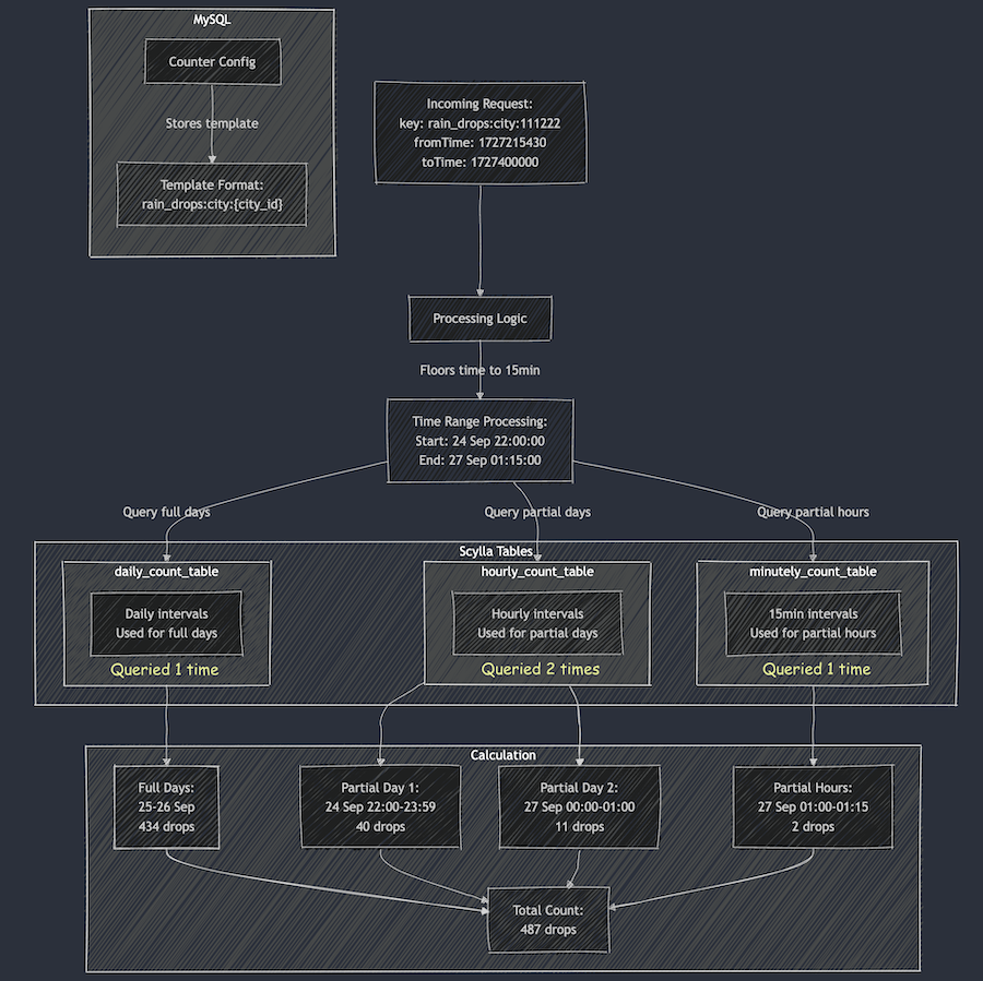
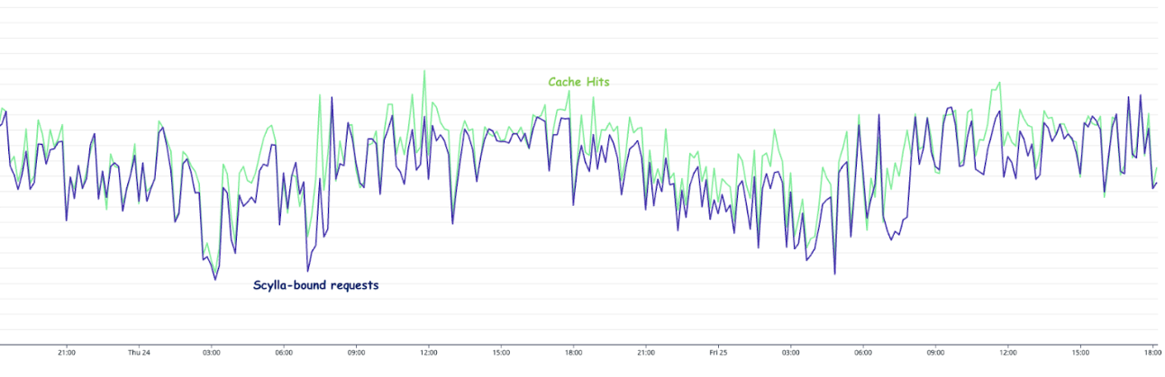
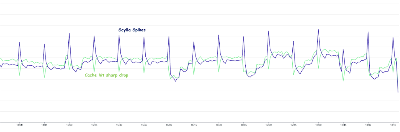
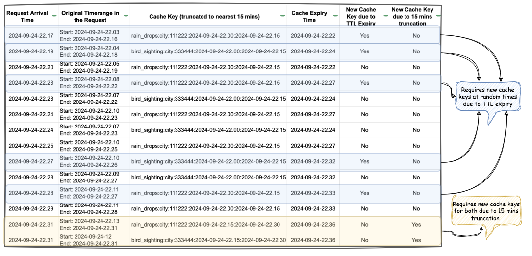
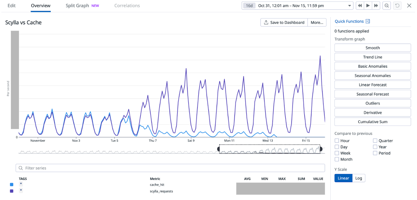
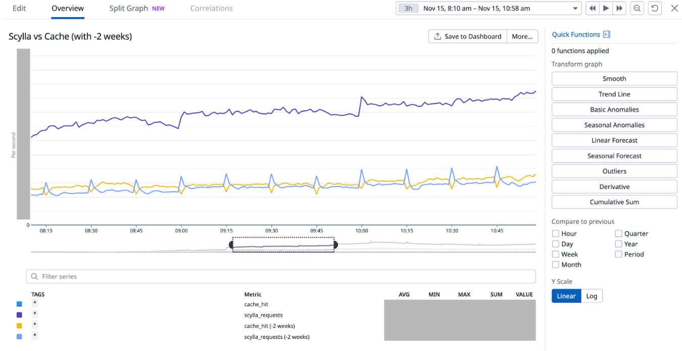
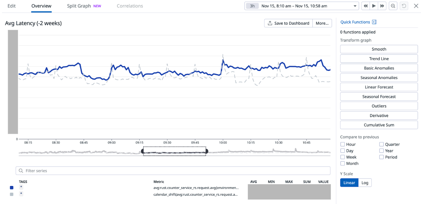
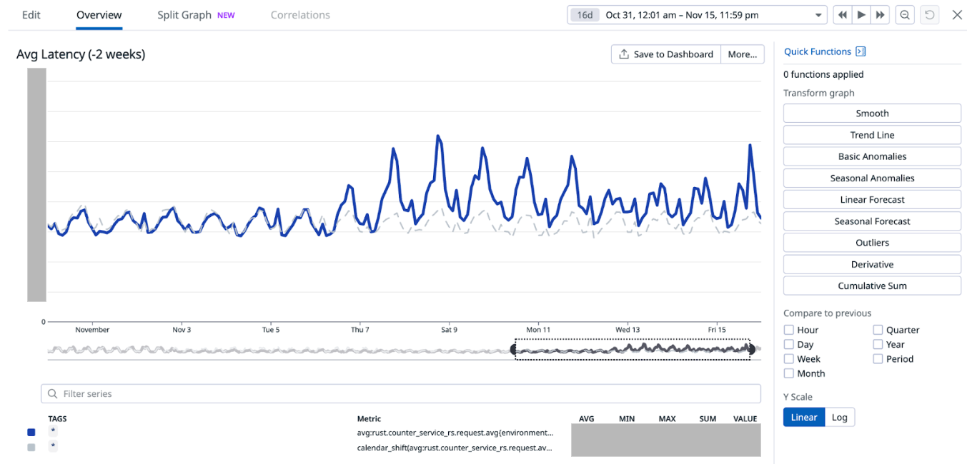
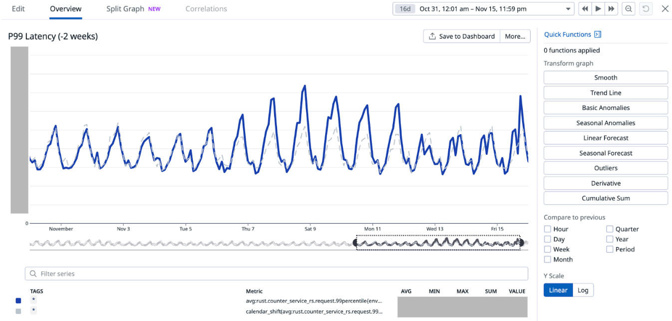
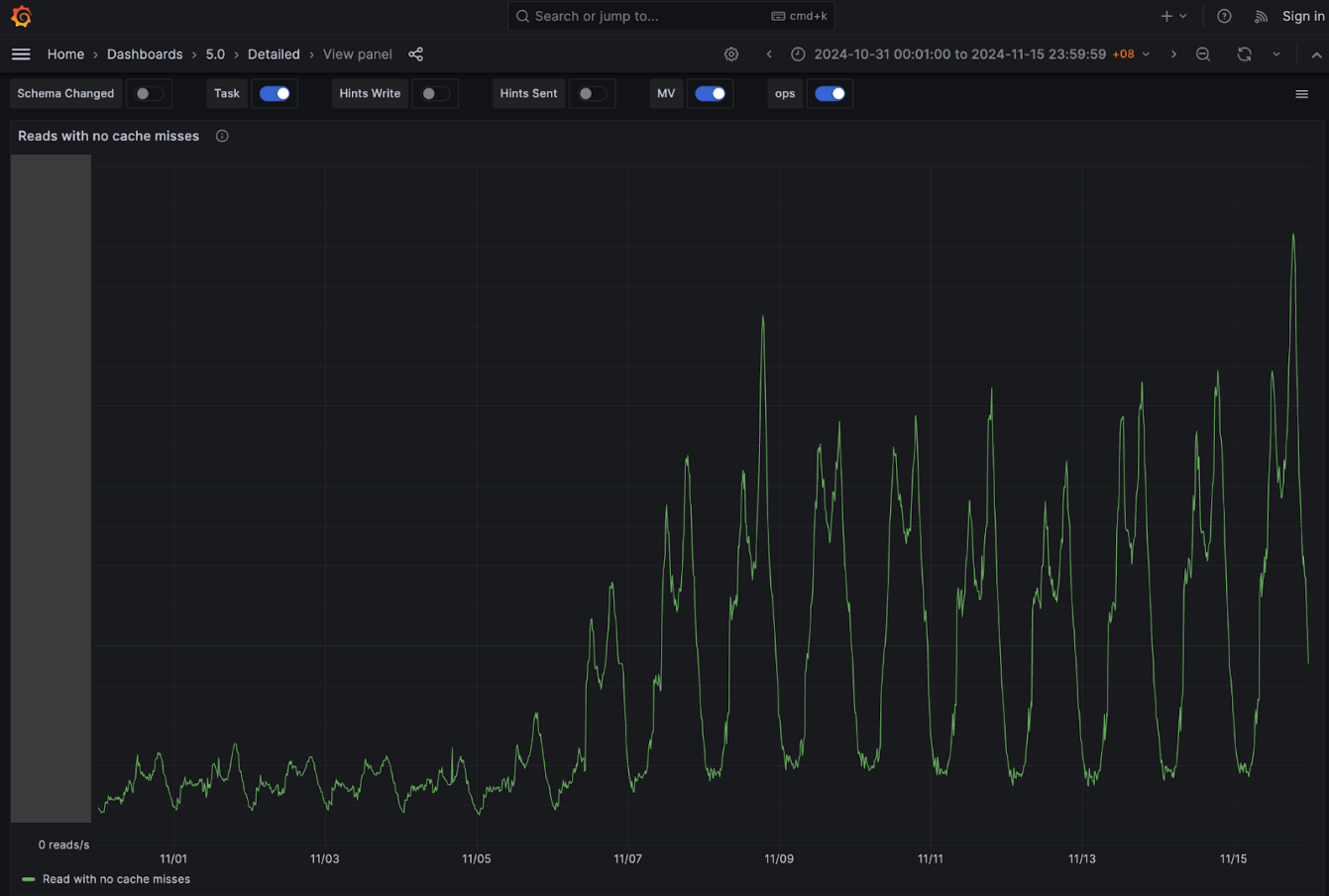
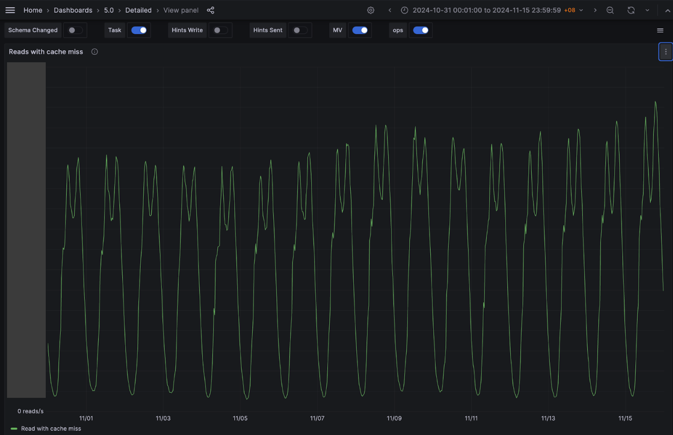
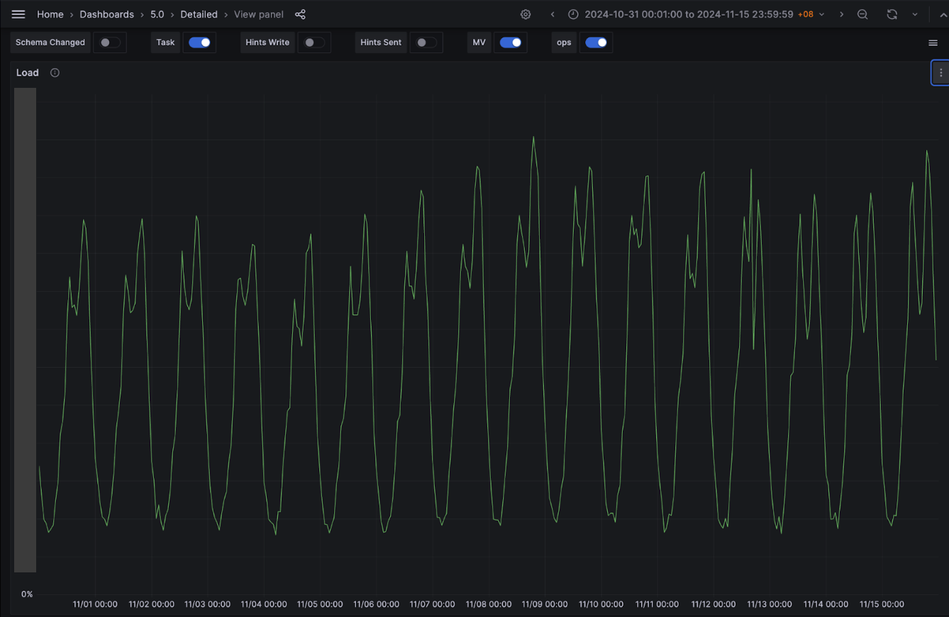
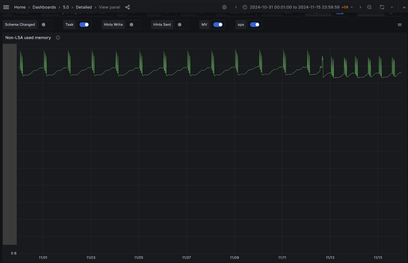











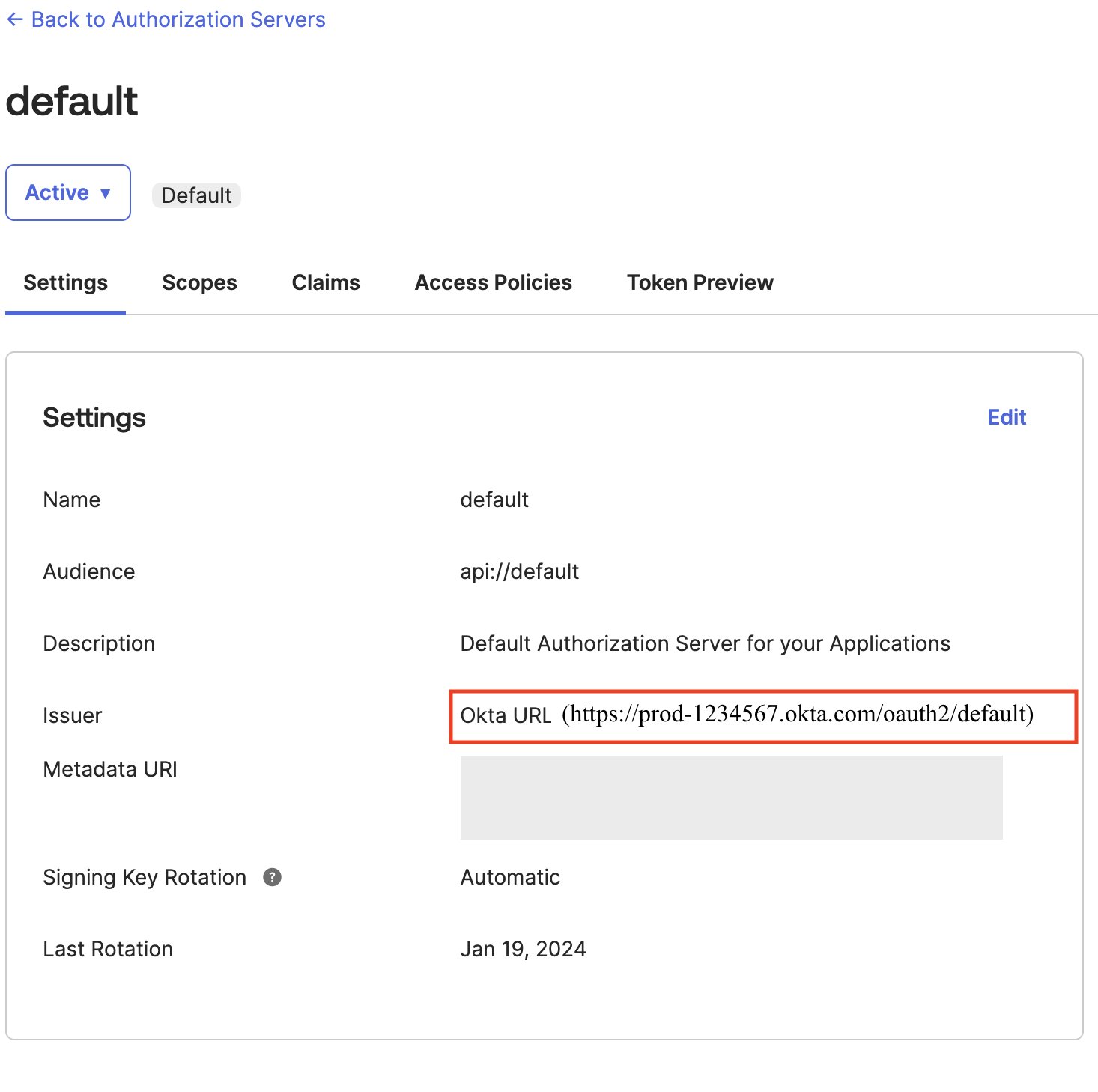


 BP Yau is a Sr Partner Solutions Architect at AWS. His role is to help customers architect big data solutions to process data at scale. Before AWS, he helped Amazon.com Supply Chain Optimization Technologies migrate its Oracle data warehouse to Amazon Redshift and build its next generation big data analytics platform using AWS technologies.
 Ali Alladin is the Senior Director of Product Management and Partner Solutions at ThoughtSpot. In this role, Ali oversees Cloud Engineering and Operations, ensuring seamless integration and optimal performance of ThoughtSpot’s cloud-based services. Additionally, Ali spearheads the development of AI-powered solutions in augmented and embedded analytics, collaborating closely with technology partners to drive innovation and deliver cutting-edge analytics capabilities. With a robust background in product management and a keen understanding of AI technologies, Ali is dedicated to pushing the boundaries of what’s possible in the analytics space, helping organizations harness the full potential of their data.