Post Syndicated from Matt Granger original https://www.youtube.com/shorts/0QNL6Mv5UrU
AWS Certificate Manager will discontinue email validation to prove domain validation for certificates
Post Syndicated from Adam Aboudi original https://aws.amazon.com/blogs/security/aws-certificate-manager-will-discontinue-email-validation-to-prove-domain-validation-for-certificates/
Today, we’re announcing that AWS Certificate Manager (ACM) will discontinue support for email-validated public certificates by September 30, 2027. If you use email validation for your ACM public certificates, you need to migrate to DNS validation before that date. This change aligns with the Certification Authority/Browser (CA/B) Forum’s industry-wide deprecation of email-based domain validation and gives you a full year to migrate ahead of the Forum’s March 2028 deadline.
In this blog post, we share the rationale for this change, the timeline, and the steps you can take to migrate your certificates to DNS validation.
Background
The CA/B Forum sets the standards that browsers and certificate authorities must follow for publicly trusted certificates. In November 2025, they voted to end support for email-based domain validation effective March 15, 2028. After that date, certificates validated through email won’t be trusted by browsers, regardless of which certificate authority issued them.
ACM will be deprecating its email validation in-line with the CA/B Forum’s requirements, by September 30, 2027. The ACM timeline gives customers one year to migrate before the CA/B Forum’s hard deadline.
Timelines for these changes
If you currently use email validation for certificates requested from ACM, there are a few important dates that you should be aware of:
- January 1, 2027: ACM will no longer offer email validation in new AWS Regions.
- March 31, 2027: ACM will no longer offer email validation for new certificate requests in any Region.
- September 30, 2027: ACM will no longer renew existing certificates that use email validation in any Region.
- March 15, 2028: Per the CA/B Forum, public certificate authorities can no longer use email-based domain validation to issue or renew publicly trusted certificates. Certificates issued before this date remain valid until they expire.
Check for existing email validated certificates
If you have any ACM issued public certificates, you can check whether any of them are email validated by using the AWS Management Console for ACM or the AWS Command Line Interface (AWS CLI).
Identify email validated certificates using the ACM console
Use the following steps in the console to find email validated certificates.
- Open the ACM console.
- Select the filters Validation method = Email and Type = Amazon Issued for a list of email validated certificates.
- Any certificates listed are public email-validated certificates and should be migrated before September 30, 2027.

Figure 1: List of all public email validated certificates
Identify email-validated certificates using the AWS CLI
Use the following commands to find email validated certificates.
Migrate existing email validated certificates
To assist you in this migration, ACM is updating the UpdateCertificateOptions API so you can switch a certificate’s validation method from email to DNS in place. This means the certificate Amazon Resource Name(ARN) will remain the same and no changes will be needed to your AWS resources that reference the certificate.
When you update a certificate to DNS validation, ACM provides a CNAME record to add to your DNS configuration, and you have 72 hours to add that record. During this window, the certificate continues to function normally on email validation. If the 72 hours elapse without a DNS update, the certificate stays active on email validation and you can retry when ready. After DNS validation is complete, ACM is designed to automatically renew your certificate before it expires without further manual intervention required. We recommend completing migration before September 30, 2027, so that ACM can keep your certificates up to date without interruption.
To migrate using the console
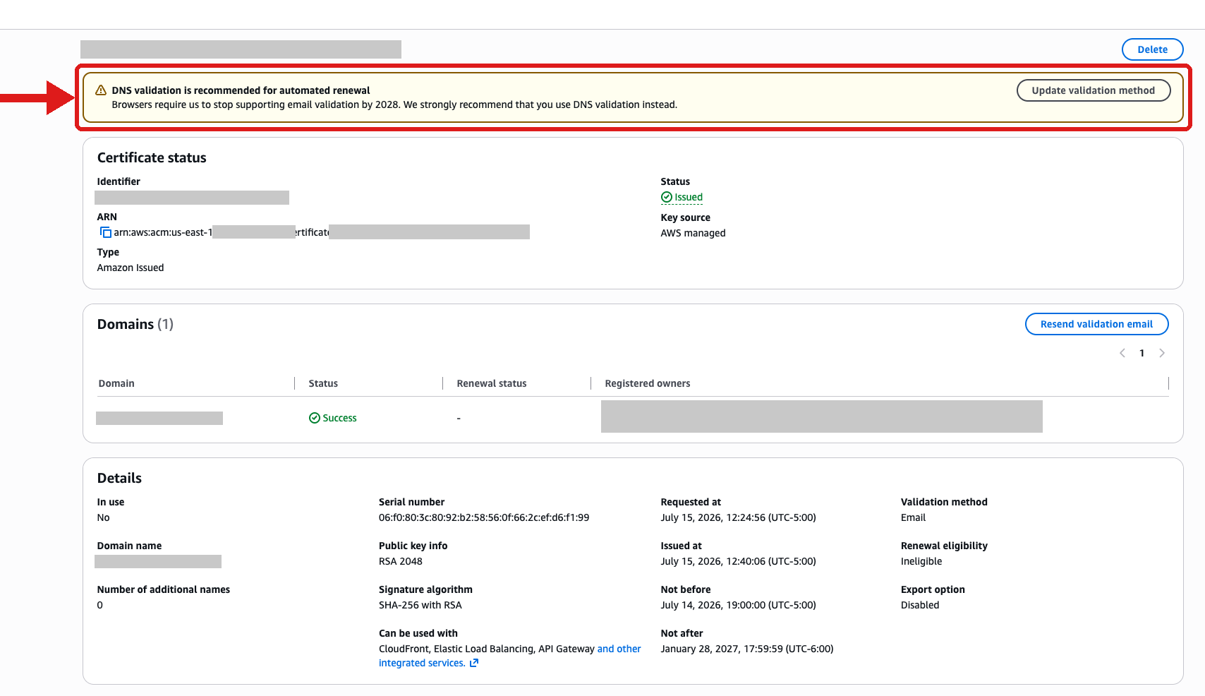
- After you’ve identified a certificate that needs updating, open it and select Update validation method at the top of the page.

Figure 2: DNS Validation prompt when viewing an email validated public certificate.
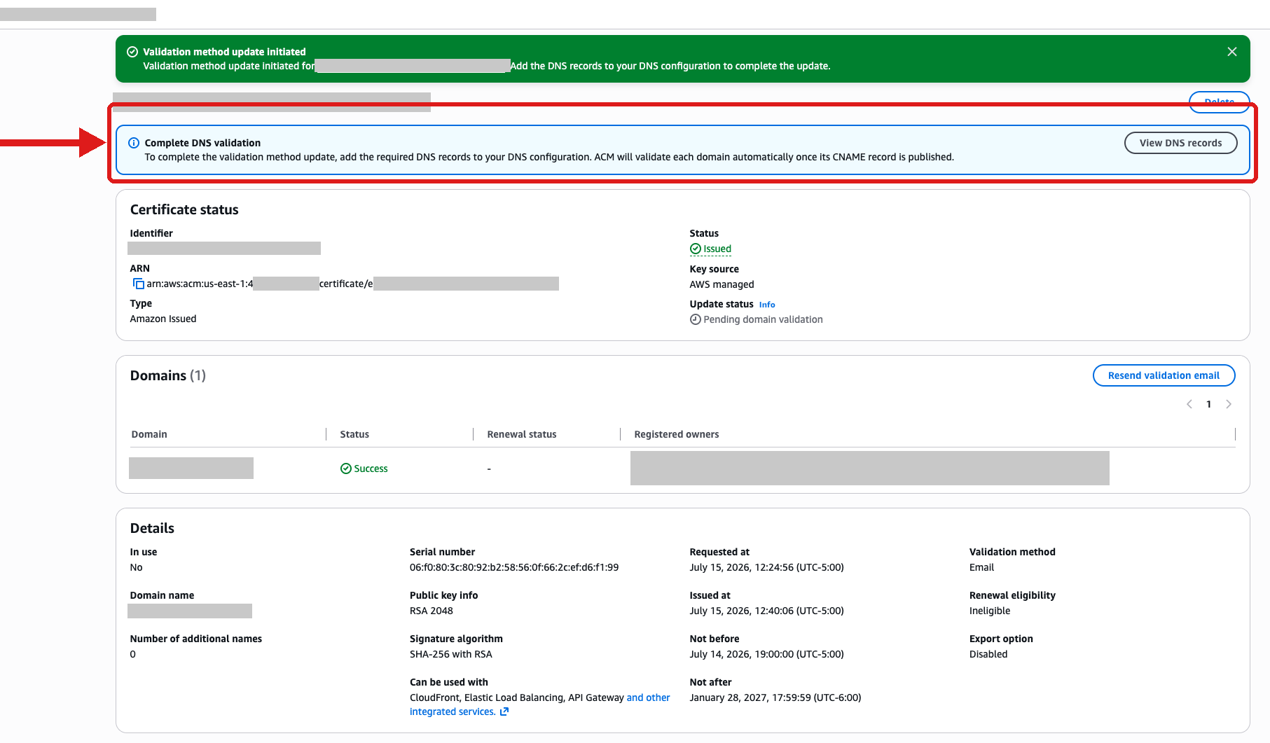
- After the update is triggered, you will see a View DNS records flashbar at the top of the certificate page.

Figure 3: View DNS validation records after updating validation method.
- Select View DNS Records in the flashbar to open a dialog box from which you can download the CSV file for the CNAME records to export to other DNS providers.

Figure 4: Get DNS validation information from the dialog box
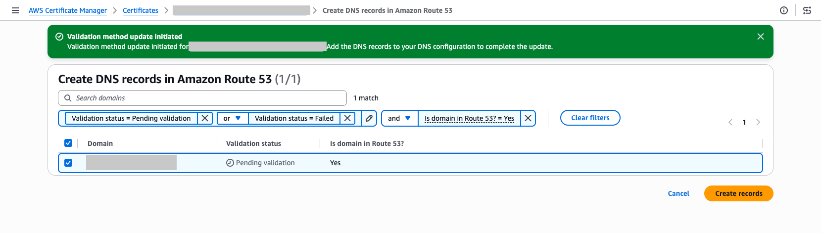
- For Route 53 users, there is a Create records in Route 53 that makes the validation available as a one-click option.

Figure 5: Create DNS validation records into Route 53

To migrate using the AWS CLI:
For instructions on how to update certificates using the AWS CLI, see the email to DNS migration user guide.
Alternatives after email validation is no longer available
ACM supports two validation methods for new certificates going forward:
- DNS validation – Add a CNAME record to your DNS configuration. ACM automatically renews DNS-validated certificates as long as the record remains in place. We recommend this method for most use cases.
- HTTP validation for CloudFront – ACM provides a unique token that you host at a well-known URL path on your domain. This method is only available for certificates used with Amazon CloudFront.
Both methods remove the manual approval step required by email validation and let ACM renew your certificates automatically.
Conclusion
The deprecation of email validation and use of the new UpdateCertificateOptions API helps keep your certificates trusted and your applications running as industry standards evolve. The updated UpdateCertificateOptions API is designed to make this migration straightforward: switch your validation method in place, add the DNS record, and ACM is designed to handle renewals automatically from that point forward.
If you have questions or need assistance migrating, contact AWS Support or start a new thread on the AWS re:Post ACM Forum.
If you have feedback about this post, submit comments in the Comments section below.
Designing for failure: Building resilient systems on AWS
Post Syndicated from Dhvani Vora original https://aws.amazon.com/blogs/compute/designing-for-failure-building-resilient-systems-on-aws/
In cloud computing, failure in distributed systems isn’t a matter of if, but when. Modern applications span servers, Availability Zones, and Regions. Each component represents a potential point of failure. Resilient applications engineer fault tolerance into their architecture, building systems that self-recover and maintain availability. This post is written for engineers and architects who run distributed data systems such as Apache Cassandra, Apache Kafka, or HDFS on Amazon Elastic Compute Cloud (Amazon EC2) and want to build resilience against hardware failure.
We were working with a customer during one such incident and wanted to share the example. The customer runs a web application that uses Cassandra as its data store, handling both read-heavy and write-heavy workloads at a scale of millions of queries per day.
The 2 AM wake-up call nobody wants
Consider a platform that monitors millions of enterprise network devices across hospitals, universities, and airports worldwide. It detects problems before IT teams even notice them. For that platform, a 2 AM page is more than inconvenient. When your value proposition is catching failures before anyone else does, being caught off-guard by your own infrastructure failure is existential.
The engineering team was deep in quarterly planning when their monitoring dashboard lit up. Three Cassandra nodes had gone dark simultaneously. This was not a graceful shutdown or a rolling restart. It was a hard failure with no warning.
Their architecture is typical of high-scale telemetry platforms. Kafka-powered microservices ingest device telemetry, Apache Flink handles real-time anomaly detection, and Apache Airflow orchestrates batch analytics and firmware updates. All of these rely on Apache Cassandra as the distributed database backbone. The database stores billions of daily writes and handles millions of queries per day.
What actually happened
Three i4i.4xlarge instances running Cassandra nodes failed simultaneously in the SFO region. Investigation revealed that all three instances were colocated on the same physical host. That host suffered a hardware failure, taking all three instances offline at once.
Engineers spent ninety minutes digging through system logs trying to determine the root cause. The root cause was architectural. The deployment lacked Partition Placement Groups, creating a single point of failure where logical replication was undermined by physical collocation.
The good news: Cassandra maintained service availability with no data loss thanks to its replication factor. The bad news: for over an hour, the system ran on a thin safety margin. One more node failure in the same replication group would have caused data unavailability for a subset of queries. That is real customer impact for a platform that promises always-on monitoring.
This is the insidious nature of correlated failures. Individual node failures are expected and designed for. That is the whole point of replication. But when your replicas share physical infrastructure, replication becomes a paper guarantee. You have three copies of the data, but they all live on the same machine.
Making matters worse, their monitoring tools completely missed the initial failure. System status checks correctly flagged the host-level problem. But without Amazon CloudWatch alarms configured to act on those checks, detection was entirely reactive. The team found out because other things started behaving oddly, not because an alarm told them three nodes were down.
Hardware fails. You can’t fix it with a patch or configuration change. The real questions are how fast you detect it, how well your system handles it, and whether failures are correlated.
How the team responded and what they changed
The operations team manually replaced two failed instances with new ones on healthy hardware and restarted the third for log collection. Once replacement instances came online, new Cassandra nodes automatically rejoined their clusters and streamed data from surviving replicas. This process took several hours depending on data volume. Only after full synchronization did the clusters return to full redundancy.
The team recognized that this ninety-minute manual scramble wouldn’t scale. Similar problems had happened before, and each time they followed the same reactive pattern: page, investigate, manually replace, wait for streaming, breathe. Here’s what they implemented to break that cycle, and what you should implement too.
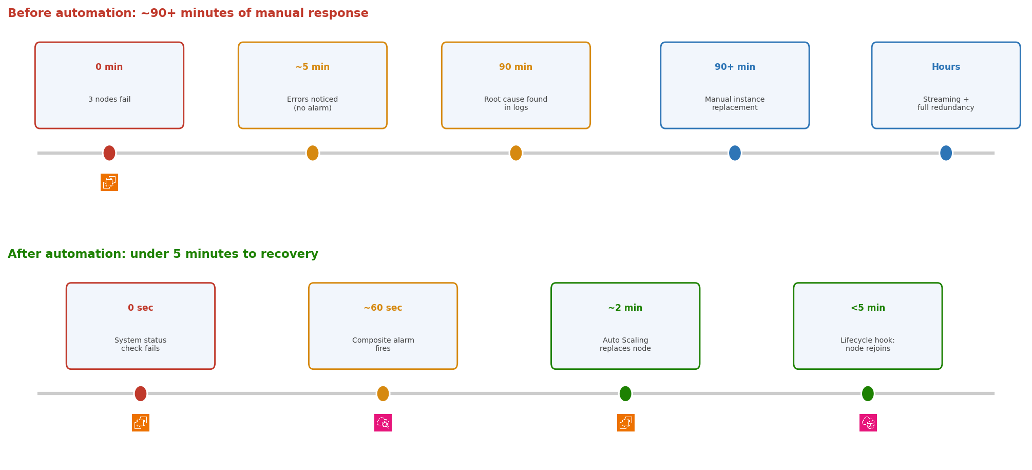
Figure 1: The same failure handled two ways. Manual response took over 90 minutes plus hours of streaming. The automated path completes recovery in under 5 minutes.
1. Use Partition Placement Groups to isolate failure domains
The three crashed servers shared a physical machine because no one told AWS otherwise. Without placement group constraints, instances are placed based on available capacity. That can mean multiple instances land on the same host. For stateless web servers, this rarely matters. For distributed databases whose entire resilience model depends on replicas being independent, it’s a silent architecture bug waiting to become a 2 AM incident.
Partition Placement Groups fix this by distributing instances across separate hardware racks. Each partition maps to a distinct set of physical infrastructure, with separate power and separate network switches. When one rack fails, it affects only the instances in that partition.
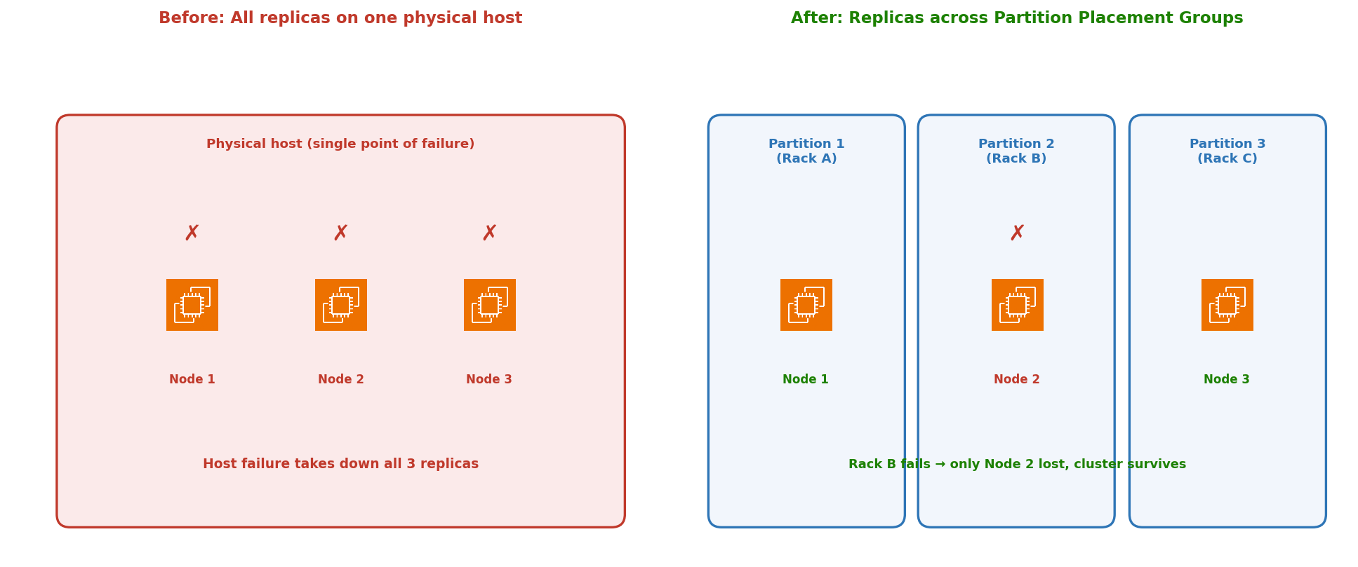
Figure 2: Distributing Cassandra replicas across Partition Placement Group partitions so a single rack failure affects only one node.
You can create up to seven partitions per Availability Zone, with as many instances as needed in each. By mapping Cassandra replicas to separate partitions, a single hardware failure takes down one node instead of three. This applies to any distributed system that maintains replicas, such as Kafka, HDFS, or Cassandra.
Key insight: Align your Partition Placement Group partitions with your application’s replication topology. If Cassandra uses a replication factor of 3, place each replica in a different partition. This means the physical isolation boundary matches the logical replication boundary.
CLI example:
Partition Placement Groups (up to 7 partitions per AZ, unlimited instances per partition) are designed for large distributed workloads. Spread Placement Groups (max 7 instances per AZ, each on a separate rack) suit small critical clusters. For a Cassandra deployment at scale, Partition is the right choice. Learn more in the Amazon EC2 placement groups documentation.
2. Monitor system status checks and use composite alarms
The Cassandra team’s monitoring blind spot came down to a distinction many teams overlook. AWS runs two health checks on every instance: instance status checks (your guest OS and software) and system status checks (the physical hardware underneath). When a system status check fails, the problem is below your control. This includes a host crash, a power failure, or network loss at the rack level. No amount of SSH-ing will help, because the box is unreachable.
The Cassandra team had no Amazon CloudWatch alarms configured on either check type. That meant the only signal was cascading application errors noticed by engineers who happened to be awake. Set these up on day one, before your first production deployment.
To avoid false alarms during normal reboots, where metrics may briefly go missing, combine system status checks with application-level health monitoring using composite alarms. When both fail together, you know there’s a real problem. See the CloudWatch composite alarms documentation for setup details.
3. Automate instance recovery and replacement
The Cassandra team’s ninety-minute recovery wasn’t slow because the engineers were incompetent. It was slow because humans were in the loop. Waking up, assessing, deciding, acting, and verifying: each step adds minutes that compound under pressure. Auto Scaling groups remove the human from the critical path.
Place your Cassandra nodes in an Auto Scaling group. Auto Scaling continuously runs health checks on every instance, and when it marks an instance unhealthy, it terminates it and launches a replacement on different physical hardware, automatically placed within your Partition Placement Group. Under normal conditions, an instance whose system status checks fail is replaced within a few minutes.
The gap to close is detection, not replacement. Rather than waiting for Auto Scaling to reach its own conclusion, have the composite alarm from the previous section explicitly tell Auto Scaling the instance is unhealthy by calling the SetInstanceHealth API. As soon as your combined signal (system status check plus application-level check) confirms a real failure, mark the instance unhealthy and let Auto Scaling replace it immediately. This sidesteps any ambiguity in detection and starts recovery in seconds rather than minutes.
For stateless services, this is enough. For stateful systems like Cassandra, you need an additional step. Lifecycle hooks pause new instances before they join the cluster. A raw Amazon EC2 instance isn’t a functioning Cassandra node. It needs to join the ring, stream data from peers, and verify consistency before serving traffic. Read more in the Amazon EC2 Auto Scaling lifecycle hooks documentation.
In this customer’s case, automating these steps cut recovery time from ninety minutes of manual intervention to under five minutes of automated recovery.
A note on stateful recovery: automated replacement only handles the infrastructure layer. For Cassandra specifically, the new node still needs to stream data from peers before it’s fully operational. The key improvement isn’t eliminating that streaming time. It’s eliminating the human response time before streaming even begins.
4. Build automated incident response with AWS Systems Manager
When servers fail, you face competing priorities. You need to replace them fast to restore capacity, and you need to preserve logs for root cause analysis. These goals conflict when done manually. The Cassandra team restarted one failed node solely to collect diagnostic data before replacing it, adding time to an already long recovery.
AWS Systems Manager runbooks automate this tradeoff away. Build a workflow that runs these steps in sequence:
- Isolate the failed instance by detaching it from the load balancer target group.
- Create an Amazon EBS snapshot and capture available logs to Amazon S3.
- Terminate the instance so that Auto Scaling can replace it.
- Notify the on-call channel with the instance ID, failure type, and Amazon S3 log location.
A subtle but important detail: when the instance’s lifecycle is managed by an Auto Scaling group, let the group replace it. Terminating the instance directly only delays recovery, because the group first has to notice the instance is gone before it launches a replacement. Instead, call the TerminateInstanceInAutoScalingGroup API. This tells EC2 Auto Scaling to terminate the unhealthy instance and immediately launch a replacement in one coordinated action. Trigger this runbook automatically with Amazon EventBridge rules that match Amazon EC2 state-change events. The result is that forensic data is preserved, replacement happens in parallel, and the on-call engineer gets a notification after the system has already healed, rather than a page asking them to start fixing it.
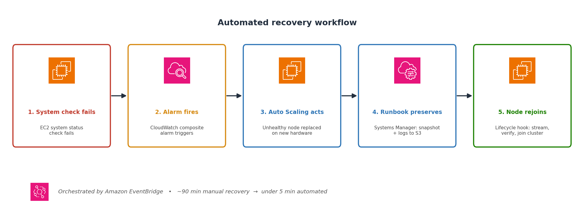
Figure 3: The automated recovery workflow, from hardware failure detection through node rejoin, orchestrated by Amazon EventBridge, Auto Scaling, and AWS Systems Manager.
5. Invest in observability before you need it
After resolving the Cassandra incident, the team asked a harder question: what else is silently failing? They ran a broader health assessment, and the answer was sobering. Unstable Redis connections were dropping under load. Amazon EBS volumes were running with elevated latency. Application Load Balancer health check intervals were misconfigured. Secondary databases were approaching connection pool exhaustion. Any of these could cause the next outage, and none of them had triggered a single alert.
This is the pattern. Teams invest in monitoring for the system that recently broke while the next failure quietly builds elsewhere. The better approach is treating observability as infrastructure. Deploy it everywhere from day one, not bolted on after the post-mortem.
Deploy the CloudWatch agent for system-level and application-level metrics. Use Amazon CloudWatch Synthetics canaries to continuously test critical user paths such as login, data ingestion, and dashboard rendering. Set up distributed tracing with AWS X-Ray to identify latency bottlenecks across your microservice mesh. The goal isn’t only knowing that services are running. It’s continuously confirming they’re working correctly from the customer’s perspective.
The Cassandra team built what they call their “resilience dashboard.” It’s a single view surfacing Partition Placement Group distribution, replica lag, system status check state, and Auto Scaling group health. When the next incident happens, they won’t be scrambling to figure out what’s broken. They’ll open one dashboard and know immediately whether their defenses are holding.
Placement groups: Quick reference
The team’s outage involved Partition Placement Groups, but Amazon EC2 offers three placement group types. Choosing the wrong one is a common mistake, so here’s how they compare:
| Type | Max instances | Isolation level | Best for |
| Partition | Unlimited (up to 7 partitions per AZ) | Separate racks per partition | Large distributed databases (Cassandra, Kafka, HDFS) |
| Spread | 7 per AZ | Each instance on a separate rack | Small critical clusters needing maximum isolation |
| Cluster | Unlimited | Same rack (co-located) | HPC, ML training, low-latency workloads |
If the Cassandra team had used Spread Placement Groups instead, they would have hit the 7-instance-per-AZ ceiling almost immediately at their scale. Partition Placement Groups gave them isolation and room to grow. For the highest-criticality deployments, combine placement groups with multiple Availability Zones. You get separate racks and separate data centers, protecting against both rack-level failures and zone-wide events like power grid outages.
The bigger picture: Resilience is a practice
Building resilient systems isn’t a one-time project. It’s a practice that evolves with your architecture. Start by assessing your workloads with the AWS Well-Architected Tool to identify single points of failure you might not see day-to-day. Define Service Level Objectives, so your team agrees on what “good enough” looks like. Not every service needs 99.99% availability, but you need to know which ones do.
Then layer your defenses. Placement groups prevent correlated hardware failures, composite alarms detect problems within minutes, and automated recovery fixes common issues without waking anyone up.
Test regularly. Run disaster recovery drills quarterly. Don’t rely only on tabletop exercises. Run actual failovers in pre-production environments. Use AWS Fault Injection Service to simulate hardware failures and zone outages in a controlled way. Hold blameless post-mortems after every incident to understand what broke, why it wasn’t caught earlier, and what you’ll change.
After this incident, the team deployed Partition Placement Groups, configured composite alarms, and automated their response process. The next time hardware fails, and it will, it won’t cause the same damage.
Consider adopting Chaos Engineering as a discipline. The principles of Chaos Engineering encourage teams to proactively inject failures into production-like environments to uncover weaknesses before they cause real outages. AWS Fault Injection Service makes it straightforward to run these experiments safely, with guardrails that automatically stop experiments if impact exceeds defined thresholds.
For related guidance, see the AWS Well-Architected Framework Reliability Pillar and the Amazon EC2 Auto Scaling User Guide. A sample Systems Manager runbook and AWS CloudFormation template for the automated recovery workflow described in this post is available in the AWS Samples GitHub repository.
If you’ve implemented similar resilience patterns or have questions about placement groups and automated recovery, share your experience in the comments.
Related posts
- Building for resilience: How Amazon EC2 Spread Placement Groups reduce correlated failures
- Automating Amazon EC2 instance remediation with AWS Systems Manager and Amazon CloudWatch
- Best practices for handling Amazon EC2 Spot Instance interruptions
- AWS Architecture Blog: Resilience
- Introducing the next generation of AWS Resilience Hub for generative AI-based SRE resilience journey
- AWS Management & Tools Blog: AWS Resilience Hub
Key takeaways
| Challenge | Solution |
| Multiple instances on same physical host | Partition Placement Groups |
| No health notification for sudden failures | Amazon CloudWatch alarms on system status checks |
| Missing metrics during host reboots | Composite alarms with application-level health checks |
| Manual, slow incident response | Automated recovery with Auto Scaling and lifecycle hooks |
| Delayed root cause identification | Systematic triage starting at the infrastructure layer |
| Reduced redundancy after failure | Auto Scaling groups for automatic replacement |
| Recurring confidence erosion | Proactive architectural reviews and observability investment |
Amazon EC2 provides tools like placement groups, managed services with built-in high availability, and automation frameworks like AWS Systems Manager. Select the right ones for your workload and test them relentlessly. Failure is inevitable. Your readiness determines the outcome.
Total eclipse of the Internet: traffic impacts in Iceland, Spain, and Portugal
Post Syndicated from Sabina Zejnilovic original https://blog.cloudflare.com/total-eclipse-internet-traffic-iceland-spain-portugal/
At a time when looking down at our devices is a ritual in daily life, a natural phenomenon that demands our attention communally upward is a welcome event. On Wednesday, August 12, a total solar eclipse swept from the North Atlantic across Europe, moving over Iceland and northern Spain and Portugal, with a deep partial eclipse over the rest of Western Europe, all near local sunset. This was the first total solar eclipse to cross mainland Europe in twenty years, and it drew millions outdoors to witness the moon pass between Earth and the sun.
As we saw during the 2026 World Cup and the last total eclipse in 2024, online behavior is noticeably affected when an event at this scale takes place. In this blog post, we’ll use data from Cloudflare Radar to examine how Internet traffic shifted alongside the moon and the sun.
Internet traffic dips align precisely with maximum obscuration
In the figure above, we measured HTTP request volume in five-minute buckets across the affected countries on eclipse day, and compared it to a normal-day baseline. Each row is a country (except for Alaska) and each column is a five-minute slice of August 12, the day of the eclipse. The countries appear above in the order in which they saw the eclipse.
The black diamonds mark the moment of maximum eclipse and the color shows the percent change in HTTP traffic versus the baseline (red = below normal, blue = above). We can see very clearly that the black diamonds overlay the darkest red, almost perfectly, signaling that as the eclipse deepened, Internet traffic decreased. The decrease was most significant along the path of totality and in countries that saw the deepest partial eclipse (Iceland, Ireland, the UK, France, Spain and Portugal) and all but absent where the sun was barely obscured (Sweden, Denmark, Poland, Switzerland).
Where the eclipse was deep, the red color and black diamonds mirror each other: traffic falls into a trough that sits directly beneath the peak of obscuration and rebounds as the sun reappears, typically within minutes of maximum coverage as people return to their screens.
The scatter plot above suggests that these decreases are not due to random chance. Each point represents the peak solar obscuration of an individual country (x-axis), against the region's traffic dip (y-axis). The traffic dip is measured as the average percentage change versus baseline in the 15-minute window surrounding maximum eclipse. The downward trend of the dotted line following the dots demonstrates that regions along the path of totality saw traffic fall by roughly 15% to 30%, whereas areas experiencing only a shallow partial eclipse dipped far less or not at all. While local variables like population density, time of day, and cloud cover account for scatter at any given coverage level, the overall direction remains consistent. Paired with the precise timing of the drops, the trend of the data demonstrates that the eclipse itself was the primary driver of the decline.
Iceland, Spain and Portugal saw the biggest decreases in traffic
The figure above shows trend lines for each individual country. The gray triangles represent the progression of the eclipse obscuration, while the red line tracks the amount of traffic changed from its usual baseline. In almost all the countries and regions impacted in the course of the eclipse, traffic made noteworthy changes ranging from 9.3 to -46.7%.
The right-hand numbers on the “y2”-axis are the obscuration, calculated using precise sun and moon positions. For each location we found the apparent angular sizes of the sun and moon and how far apart they are in the sky, then calculated the fraction of the sun's disk covered by the moon every 5 minutes via the geometric overlap of two circles. That gave each place both its peak obscuration (how deep the eclipse got, 0–100%) and its moment of maximum eclipse. We then summed all regions in each country for the traffic total, and took the average obscuration across a country's regions to place its national max-eclipse time.
To differentiate the eclipse from a typical Wednesday evening, we compared eclipse day against the same weekday: the median of the three previous Wednesdays, matched slot-by-slot on time-of-day. Using the median keeps one odd week from skewing the comparison. Every number is then reported as percent change vs. baseline. When looking at the percentage on the left-hand y-axis, 0% means "totally normal" and negative means "less active than usual."
We can see the changes in traffic beginning in Alaska around 15:35 UTC, where the eclipse began its pathway. Iceland, Spain, and Portugal experienced the most dramatic drops in traffic, whereas Poland and Denmark quickly returned to pre-eclipse levels. Norway and Sweden actually saw slight traffic increases above baseline, while Denmark recorded the least overall change.
Ultimately, these findings reveal a clear correlation between the path of the eclipse and human behavior online. While the severity and duration of traffic drops varied by region, Radar’s HTTP traffic data demonstrates how a shared physical event can temporarily reshape digital activity across an entire continent.
Track the impact of world events on Cloudflare Radar
Major events in the physical world remind us that digital traffic is, at its core, a direct reflection of human attention. When the moon obscured the sun across Europe, the Internet slowed down not because of network failures, but because people paused their online activity to watch. As network patterns quickly normalized post-eclipse, the data left behind offers a fascinating snapshot of how a cosmic event can momentarily realign our online world.
To explore more interactive traffic insights and track how major worldwide events shape internet activity every day, visit Cloudflare Radar or follow us on social media at @CloudflareRadar (X), https://noc.social/@cloudflareradar (Mastodon), and @radar.cloudflare.com (Bluesky).
Domas: Bypassing memory protection with AMD’s memory controllers
Post Syndicated from daroc original https://lwn.net/Articles/1088778/
Christopher Domas has
published a proof of concept with a description showing how to use AMD memory controllers’ bank swizzle mode to bypass memory protection and read or write arbitrary data, including CPU microcode definitions and memory belonging to the
platform security processor. Among other things, this allows code running at the kernel level to directly manipulate the meaning of processor instructions, potentially bypassing other security measures such as memory encryption and virtual machine isolation.
This is not, strictly, unexpected behavior: it is
documented in AMD’s manual (on page 113 of that PDF). But the fact that it can be used to access arbitrary memory and thereby rewrite supposedly immutable parts of the computer’s firmware without crashing the host machine seems like an unintentional side-effect of the design. Fortunately, since enabling bank swizzle mode requires kernel-level privileges, the vulnerability is not an immediate problem for most software. Still, it seems likely that this technique will end up being used for nefarious purposes eventually.
Will There Be a Migration Away from the GOP?
Post Syndicated from The Atlantic original https://www.youtube.com/shorts/_BKW7UEA6EM
Microchip Switchtec 160-Lane PCIe Gen6 Switch Shown at FMS 2026 with XpressConnect PCIe 6 Retimer
Post Syndicated from Patrick Kennedy original https://www.servethehome.com/microchip-switchtec-160-lane-pcie-gen6-switch-shown-at-fms-2026-with-xpressconnect-pcie-6-retimer/
At FMS 2026, we saw a 160-lane Microchip Switchtec PCIe Gen6 switch, XpressConnect retimer demo, and even an Everpure cameo
The post Microchip Switchtec 160-Lane PCIe Gen6 Switch Shown at FMS 2026 with XpressConnect PCIe 6 Retimer appeared first on ServeTheHome.
The Night My Marriage Fell Apart
Post Syndicated from The Atlantic original https://www.youtube.com/shorts/YnW0IIDx_9w
S10 E3: Ron DeSantis & Radiant Plumbing: Last Week Tonight with John Oliver
Post Syndicated from LastWeekTonight original https://www.youtube.com/watch?v=Ex9FKp7FPMw
Track generative AI costs with Amazon Bedrock inference profiles
Post Syndicated from Erik Mack original https://aws.amazon.com/blogs/architecture/track-generative-ai-costs-with-amazon-bedrock-inference-profiles/
Tracking generative AI costs is a common challenge when multiple teams share a single foundation model through Amazon Bedrock. Your HR team answers policy questions, Accounting analyzes financial documents with it, and IT troubleshoots infrastructure issues. All three use the same foundation model. But usage shows up as one line item on the bill. As a result, finance can’t charge back each department, set per-team budgets, or identify who’s driving the most spend.
With Amazon Bedrock application inference profiles, you can solve this. An inference profile is a tagged wrapper around a foundation model. You can use it to attribute costs to specific teams or departments. By combining these profiles with AWS cost allocation tags, you can view per-department Amazon Bedrock costs as separate line items in AWS Cost Explorer.
In this post, we show you how to create application inference profiles for three departments and tag them for cost allocation. You also update your application to route invocations through department-specific profiles and view the per-department cost breakdown in Cost Explorer.
Solution overview
The following diagram shows the solution architecture. Users authenticate at the application layer, and the application identifies each user’s department. It then routes the request to that department’s tagged inference profile in Amazon Bedrock. All profiles use the same foundation model. The application calls Amazon Bedrock using a single IAM role, and individual user identities are not passed to AWS. Cost attribution comes from the inference profiles rather than the calling identity. Amazon Bedrock records usage against each profile’s Team tag, and AWS Cost Explorer displays the costs grouped by department.
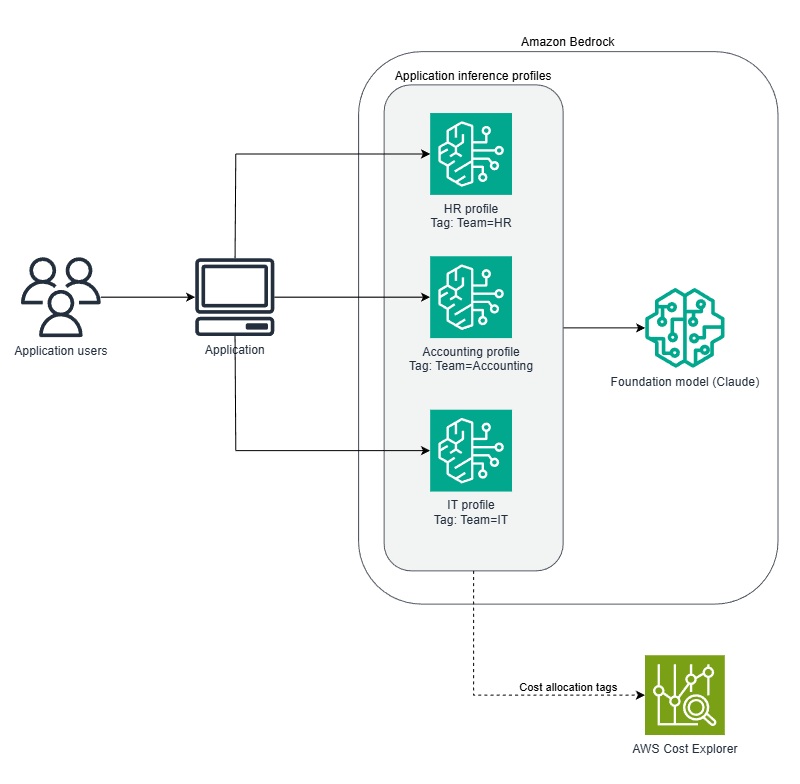
Figure 1 — Solution architecture for per-department cost tracking with application inference profiles
Amazon Bedrock can also attribute inference costs to the IAM principal that makes each call. This works well when each team calls Amazon Bedrock under a distinct IAM identity. In this architecture, a single application serves all departments under one role. Per-caller attribution can’t separate team costs without adding per-user session management. With application inference profiles, you can attribute costs per team by routing each team to a tagged profile.
To track costs per department:
- Create an application inference profile for each department, associating each one to the same foundation model.
- Tag each profile with a cost allocation tag (for example,
Team=HR). - Activate the tag in the AWS Billing and Cost Management console.
- Update your application to route invocations through each department’s inference profile Amazon Resource Name (ARN).
- View the per-department cost breakdown in Cost Explorer.
You pay the same per-token rate whether you invoke the model directly or through an inference profile – no additional charges for cost attribution.
Create and configure inference profiles for cost tracking
The following sections walk you through creating inference profiles, activating cost allocation tags, updating your application, and viewing costs in Cost Explorer.
Prerequisites
To configure this solution, you need the following:
- An AWS account.
- Model access enabled for your chosen foundation model in Amazon Bedrock (for instructions, refer to the Amazon Bedrock User Guide).
- AWS Identity and Access Management (IAM) permissions including
bedrock:CreateInferenceProfile,bedrock:TagResource,bedrock:InvokeModel,bedrock:InvokeModelWithResponseStream,ce:GetCostAndUsage, andce:UpdateCostAllocationTagsStatus. - Access to the AWS Billing and Cost Management console to activate cost allocation tags and view Cost Explorer. For more information, refer to Managing access permissions for AWS Billing.
- Python 3.12 with boto3 1.35.7 or later (for testing invocations).
Estimated time: 30 minutes (plus 24–48 hours for cost data to appear in Cost Explorer).
Estimated cost: Based on invocations at standard model pricing. For more information, refer to Amazon Bedrock Pricing.
Create application inference profiles
Create an application inference profile for each department. Each profile points to the same foundation model but has a unique tag for cost tracking.
To create an application inference profile:
- On the Amazon Bedrock console, in the navigation pane, choose Inference profiles.
- Choose the Application tab.
- Choose Create inference profile.
- For Profile name, enter HR.
- For Model, select your foundation model (for example, Anthropic Claude).
Note: Model availability varies by Region. Check the Amazon Bedrock model availability documentation for the current list.
To tag the inference profile:
- In the Tags section, choose Add tag.
- For Key, enter Team.
- For Value, enter HR.
- Choose Create. The inference profile status changes to Active.
- Repeat for Accounting (Tag:
Team=Accounting) and IT (Tag:Team=IT).
The following figure shows the create inference profile page with the profile name and tag configured.
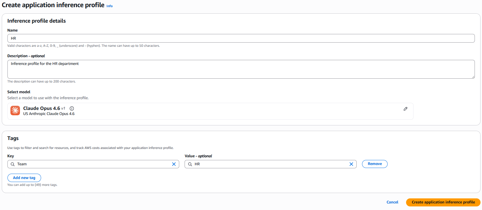
Figure 2 — Creating an application inference profile with a department tag
After you create all three profiles, the Application inference profiles list shows the HR, Accounting, and IT profiles, each with a status of Active and its corresponding Team tag. The following figure shows the three inference profiles after creation.
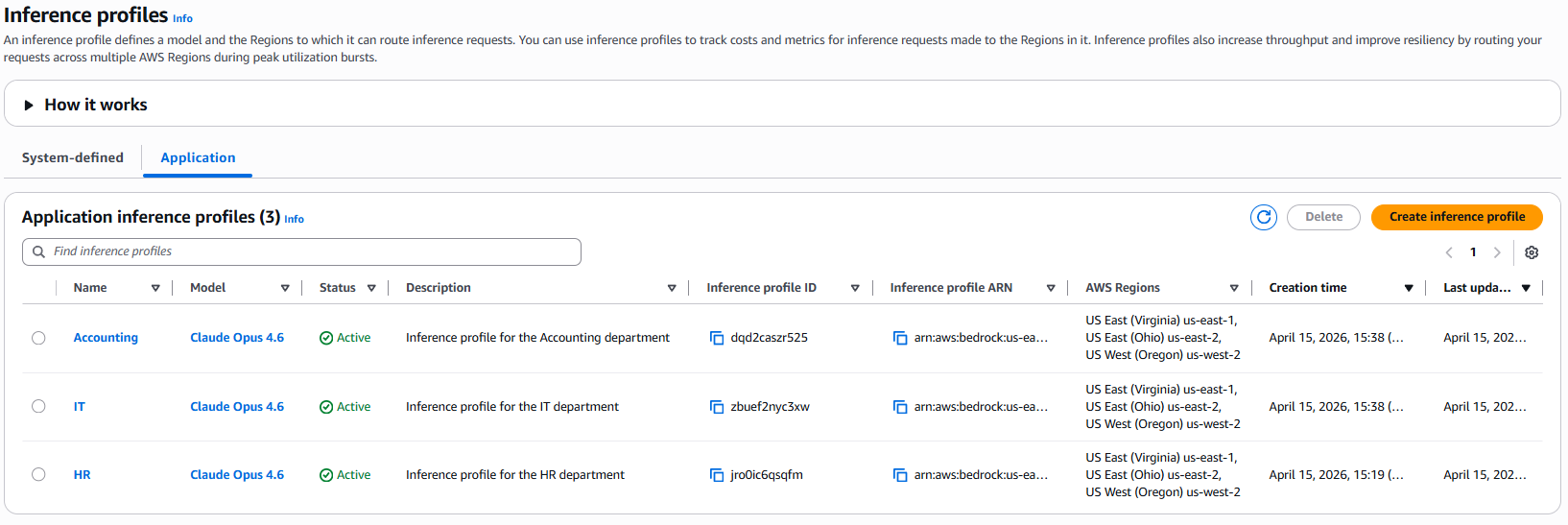
Figure 3 — Three application inference profiles, one per department
To provision inference profiles at scale (for example, one per team across dozens of teams), use the AWS::Bedrock::ApplicationInferenceProfile AWS CloudFormation resource instead of creating each profile manually.
Activate the cost allocation tag
After creating the inference profiles, you activate the cost allocation tag so that tagged costs appear in Cost Explorer. In multi-account environments using AWS Organizations, activate the Team cost allocation tag in the management (payer) account. Tagged usage from member accounts then consolidates in Cost Explorer. For more information about cost allocation tags, refer to Using AWS cost allocation tags.
To activate the cost allocation tag:
- Open the AWS Billing and Cost Management console.
- In the navigation pane, choose Cost allocation tags.
- In the search box, enter Team.
- Select the Team tag.
- Choose Activate.
The tag status changes to Active.
Note: Cost allocation tags are case-sensitive. Team and team are different tags. Tagged costs can take 24–48 hours to appear in Cost Explorer after activation.
Update the application to use inference profiles
To attribute costs to a department, pass the inference profile ARN as the modelId parameter instead of the foundation model ID. The API call remains the same. You only change the ID you pass.
To find an inference profile ARN:
- On the Amazon Bedrock console, choose Inference profiles.
- Select the profile.
- Copy the ARN from the details panel.
The ARN appears in the format arn:aws:bedrock:region:account-id:application-inference-profile/profile-id.
The following example shows how to route invocations based on the user’s department:
The full code is available on the GitHub repo.
When using inference profiles in production, validate user inputs and consider using Amazon Bedrock Guardrails to filter unintended content. API communications with Amazon Bedrock are encrypted in transit using Transport Layer Security (TLS). For more information about data protection, refer to Data protection in Amazon Bedrock.
Configure the IAM policy for Amazon Bedrock access
Because a single application calls Amazon Bedrock on behalf of all departments, it uses one IAM role. The following policy grants that role permission to invoke the department inference profiles and the underlying foundation model:
The wildcard (*) in the application inference profile ARN lets the single application role invoke the department profiles. The foundation model ARN is required because invoking through an inference profile needs permissions on both the profile and the underlying model. The application determines which department each request belongs to and routes it to the matching profile, and cost attribution comes from each profile’s Team tag. To further restrict access, replace the wildcard with the specific ARNs of your profiles.
Replace 111122223333 with your AWS account ID in the preceding policy.
To create the policy:
- On the IAM console, choose Policies.
- Choose Create policy.
- Choose the JSON tab.
- Paste the preceding policy.
- Choose Next.
- For Name, enter BedrockDepartmentAccessPolicy.
- Choose Create policy.
The BedrockDepartmentAccessPolicy appears in the policies list.
To attach the policy to a role:
- In the navigation pane, choose Roles.
- Select the role used by your application.
- Choose Add permissions.
- Choose Attach policies.
- Search for BedrockDepartmentAccessPolicy.
- Select BedrockDepartmentAccessPolicy.
- Choose Add permissions.
The BedrockDepartmentAccessPolicy appears in the role’s permission list. To add a department later, create another tagged inference profile and map it in your application. With the wildcard policy, no IAM change is needed. If you scoped the policy to specific ARNs, add the new profile’s ARN.
View per-department costs in Cost Explorer
To view the per-department breakdown in Cost Explorer:
- Open the Billing and Cost Management console.
- In the navigation pane, choose Cost Explorer.
- Set the date range to cover the period after you ran invocations.
- For Granularity, select Daily or Monthly.
- Choose Group by.
- Select Tag.
- Select Team.
To view exact amounts, scroll down to view the cost breakdown table.
The following figure shows the per-department cost breakdown in Cost Explorer. The bar chart displays a separately-colored segment for each department – HR, Accounting, and IT – with the cost amount for each. The table below the chart lists the exact dollar amount per department for the selected time period.
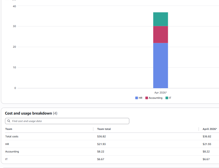
Figure 4 — Per-department Amazon Bedrock costs in Cost Explorer, grouped by the Team tag
After running invocations through each inference profile, verify the following:
- Each inference profile shows the correct
Teamtag in the Amazon Bedrock console. - The
Teamcost allocation tag is active in the Billing and Cost Management console. - Per-department costs appear in Cost Explorer when you group by the
Teamtag.
If costs don’t appear after 48 hours, verify that the cost allocation tag is active and that invocations were made through the inference profile ARNs. If invocations fail, confirm that the inference profile status is Active and the IAM role has the required permissions.
Clean up
Inference profiles don’t incur charges on their own. You only pay for model invocations made through them. As a cleanup step, delete the inference profiles you created for this walkthrough to prevent accidental invocations.
Note: Deleting an inference profile immediately affects applications using that profile ARN. Verify that applications are not actively using these profiles before deletion. To recover, recreate the profile — note that it receives a new ARN, so update your application references.
Delete the following resources:
- Application inference profiles – For instructions, refer to Delete an application inference profile.
- IAM policy – For instructions, refer to Deleting IAM Policies.
Teamcost allocation tag – Deactivate it in the Billing and Cost Management console. For instructions, refer to Deactivating cost allocation tags.
Conclusion
In this post, we showed you how to split generative AI costs by team using Amazon Bedrock application inference profiles and cost allocation tags. With this approach, you can see each department’s costs as a separate line item in Cost Explorer.
To add a new department, create another tagged profile. Costs show up as a separate line item.
You can also:
- Set per-department spending alerts and control with AWS Budgets.
- Detect unusual spending patterns with AWS Cost Anomaly Detection.
- Monitor token usage per department with Amazon CloudWatch.
- Attribute costs for higher-level Amazon Bedrock features – reference the same tagged profile ARN in the Knowledge Bases (RAG) to extend per-team attribution beyond direct model invocation.
For more background on application inference profiles, refer to Track, allocate, and manage your generative AI cost and usage with Amazon Bedrock.
For more information about inference profiles, refer to the Amazon Bedrock User Guide.
For help implementing this solution, contact your AWS representative.
About the author
How AppFolio transformed its data streaming architecture with Amazon MSK Express brokers
Post Syndicated from Brandon Stanley original https://aws.amazon.com/blogs/big-data/how-appfolio-transformed-its-data-streaming-architecture-with-amazon-msk-express-brokers/
Real-time data streaming and event processing are critical components of modern distributed systems architectures. Apache Kafka has emerged as a leading platform for building real-time data pipelines and enabling asynchronous communication between microservices and applications. However, running and managing Kafka clusters at scale can be challenging, requiring specialized expertise and significant operational overhead.
Amazon Managed Streaming for Apache Kafka (Amazon MSK) is a fully managed service that you can use to build and run production Kafka applications. With Amazon MSK, you can rely on AWS to handle the heavy lifting of provisioning and managing Kafka clusters, while you focus on building innovative applications and real-time data processing pipelines.
In this post, you learn how AppFolio adopted Amazon MSK Express brokers to replace hours-long rebalances and manual storage planning with a streaming platform that scales automatically.
About AppFolio and its data streaming platform
AppFolio is a leading Real Estate Performance Management platform, serving thousands of property management companies across the United States. AppFolio’s platform processes millions of transactions daily, from rent collection and maintenance requests to lease management and financial reporting. In this data-intensive environment, reliable streaming infrastructure isn’t only important. It’s mission-critical.
At AppFolio, real-time data is the foundation of the company’s ability to deliver powerful, intelligent solutions that power the real estate industry. To achieve this level of performance, AppFolio engineered a modern streaming data architecture built on Amazon MSK with Express brokers. This infrastructure enables high-throughput, real-time applications at scale. With Amazon MSK Express brokers, AppFolio reliably ingests massive volumes of diverse data, including Change Data Capture (CDC) and server-side events, and makes it available to downstream consumers, such as real-time fraud detection, financial reporting, and automated property management workflows, within seconds of origin.
Previous architecture and AppFolio’s evolving requirements
Until early 2025, AppFolio ran their streaming platform on a single Amazon MSK cluster with Standard brokers, supporting both customer-facing and internal workloads. The architecture served them well through earlier growth phases. As AppFolio’s data platform evolved to support increasingly complex use cases and higher throughput, two characteristics of their workload led them to look for a more elastic streaming foundation.
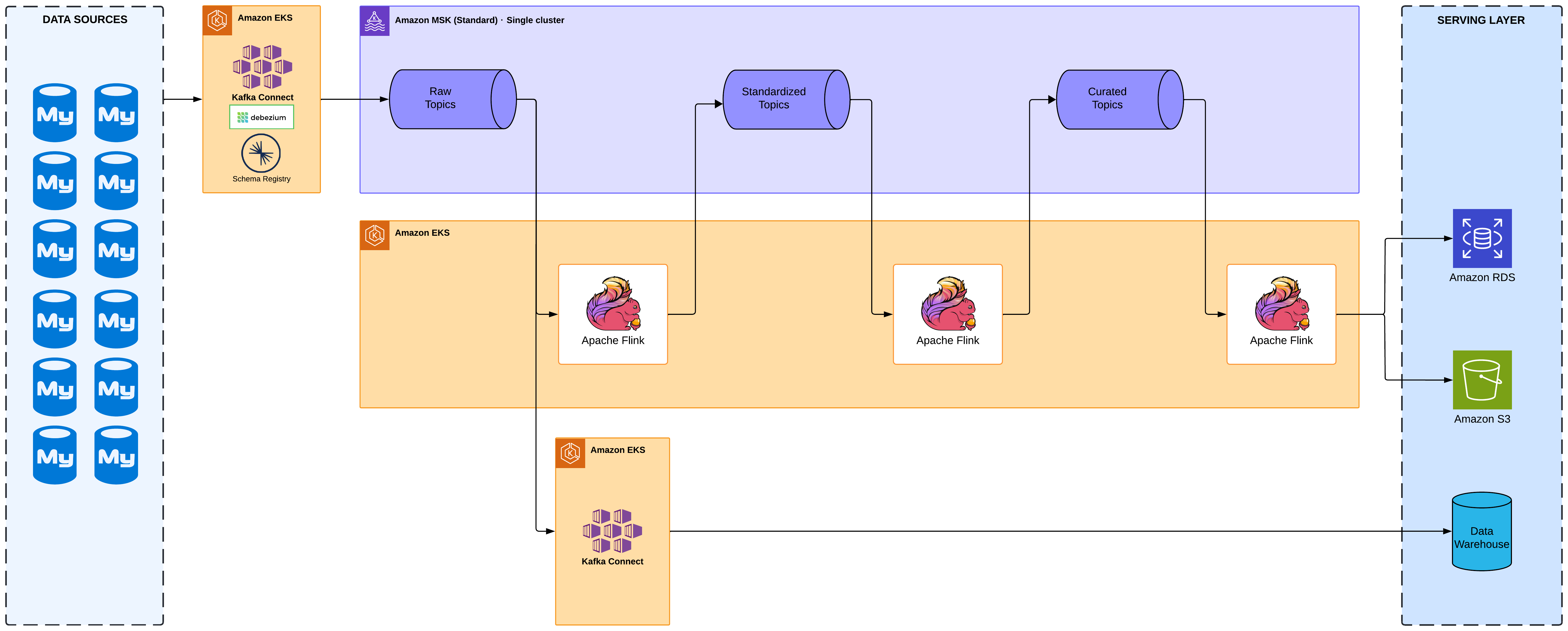
Figure 1: AppFolio’s previous architecture with Amazon MSK Standard brokers
First, AppFolio makes extensive use of log-compacted topics for their CDC streams. Compacted topics retain the latest value for each key indefinitely, which is exactly what they want for streams that mirror the state of operational tables. As their footprint grew, AppFolio wanted an infrastructure model that could scale storage automatically alongside data growth, without ongoing capacity planning that took multiple hours every month.
Second, AppFolio’s throughput continued to grow as they onboarded new use cases and added more event sources. They wanted the ability to scale the cluster quickly in response to traffic shifts, with minimal lead time for partition reassignments.
Third, as AppFolio’s platform matured, they needed workload isolation between customer-facing and internal data flows. Running customer-facing and internal workloads on a single cluster made it harder to size and tune each independently. As both grew, AppFolio wanted dedicated resources so each could be sized and tuned independently.
Based on these needs, AppFolio identified the following key requirements for their next-generation streaming platform:
- Elastic, automatically managed storage that scales with AppFolio compaction-heavy CDC workloads, removing the need for upfront broker capacity planning.
- Faster horizontal scaling and partition reassignment so AppFolio can adjust cluster shape in response to actual traffic in minutes rather than hours.
- Workload isolation between customer-facing and internal data flows, so each workload can be sized and tuned for its own traffic pattern.
Why AppFolio chose Amazon MSK Express brokers
After evaluating their options, AppFolio chose Amazon MSK Express brokers as the foundation for their next-generation streaming platform. Express brokers are a broker type offered under MSK Provisioned. They include pay-as-you-go elastic storage that scales automatically, intelligent partition rebalancing, and Kafka configuration defaults tuned for production workloads. Express brokers mapped directly to the requirements AppFolio identified:
- Elastic storage that scales with their data. Express brokers remove broker disk sizing and provisioning, with storage scaling automatically alongside data growth. AppFolio pays only for the storage actually used.
- AWS benchmarks showed up to 20 times faster scaling. Horizontal scaling and partition reassignment that previously took hours now complete in minutes, letting AppFolio react to traffic shifts on a much shorter cycle.
- Production-tuned defaults. Express brokers come pre-configured with Kafka best-practice defaults and built-in client throughput quotas, simplifying AppFolio’s operational model.
- Full Kafka API compatibility. AppFolio was able to migrate without changes to its producer and consumer applications.
As part of the migration, AppFolio also took the opportunity to rethink how the cluster was being used. Rather than recreating a single shared cluster on Express brokers, they segmented their MSK clusters by workload type. This gives customer-facing and internal workloads dedicated resources, providing better isolation and more predictable performance for each workload class.
Current architecture
AppFolio’s current architecture consists of multiple Amazon MSK clusters with Express brokers, segmented by workload type. Each cluster is sized and tuned for its specific traffic pattern, providing improved isolation and more predictable performance. The following diagram shows the deployment.
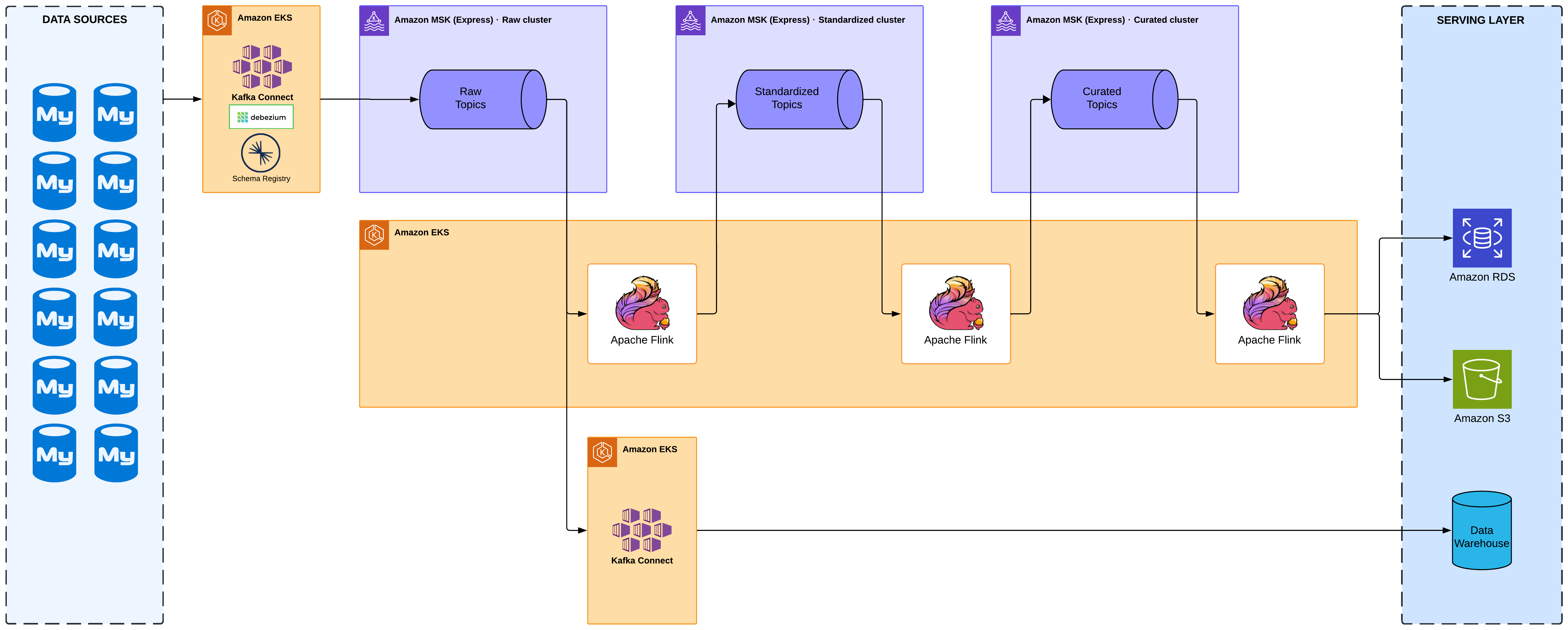
Figure 2: Current architecture with workload-segmented Amazon MSK clusters using Express brokers
Benefits achieved
By migrating to Amazon MSK Express brokers and adopting a workload-segmented cluster design, AppFolio has realized several key benefits:
Elastic, hands-off storage
The pay-as-you-go storage of Express brokers scales automatically with AppFolio’s data growth. Storage capacity is no longer something the platform team plans, provisions, or monitors, and AppFolio pays only for what they use. For a workload that runs heavily on compacted topics, this is the single largest operational improvement they have seen.
Faster scaling
Partition reassignment and broker scaling that previously took hours now complete in minutes, enabling AppFolio to adjust cluster shape in response to actual traffic instead of running ahead of forecasts.
Improved workload isolation
Splitting their streaming traffic into workload-segmented clusters has given AppFolio more predictable performance. Customer-facing and internal workloads now run on dedicated infrastructure, and each cluster can be sized and tuned for its own traffic pattern.
Stable environment as data volumes grow
Since the migration, AppFolio has maintained a stable environment with no significant downtime, even as data volumes continue to grow.
Reduced operational overhead
Hands-off storage management and intelligent rebalancing have removed several recurring tasks from the AppFolio platform team’s queue, including the constant monitoring and manual intervention that storage planning required under their previous architecture.
Conclusion
By using Amazon MSK Express brokers and adopting a workload-segmented cluster design, AppFolio has built a streaming foundation that scales elastically with their data growth and adapts quickly to changes in traffic. The pay-as-you-go storage and faster scaling of Express brokers let AppFolio’s platform team focus engineering effort on building new capabilities for customers, rather than on Kafka capacity planning. As AppFolio continues to expand its platform for the real estate industry, the Amazon MSK Express brokers infrastructure provides a scalable foundation for future growth.
To learn more about Express brokers for Amazon MSK, see the Express brokers for Amazon MSK documentation and the AWS announcement post Introducing Express brokers for Amazon MSK.
About the authors
Backblaze Drive Stats: How an Open Dataset Powers Academic and AI/ML Research
Post Syndicated from Stephanie Doyle original https://www.backblaze.com/blog/backblaze-drive-stats-academic-ai-ml-research/

Since April 2013, Backblaze has published the daily health readings of every hard drive running in our data centers. Model, serial number, failure flag, and dozens of Self-Monitoring, Analysis, and Reporting Technology (SMART) attributes, collected into a CSV for each day, released publicly every quarter, for free. We built Drive Stats as a mechanism to understand our own fleet, then published almost on a whim—so much so that the original idea is credited to two Brians. What happened next was an exciting surprise.
More than 227 papers and articles have cited Drive Stats as a primary dataset since 2018. Researchers have trained transformer architectures, long short-term memory (LSTM) networks, survival models, and gradient-boosted ensembles on it. The dataset that started as an internal reliability tool has become one of the most-cited open benchmarks in hard drive failure prediction research.
What makes Drive Stats so valuable?
Drive Stats reflects a live, continuously operating commercial fleet of drives: different manufacturers, different models, different capacities, all spinning in production Storage Pods under real workload conditions. That combination of scale and heterogeneity is rare, and it is exactly what makes the dataset especially useful to researchers.
For storage engineers and data scientists, the dataset checks every important box: real-world origin, a long time horizon, labeled failures, an open license, and an active maintainer that publishes new data each quarter. Here are a few other specifics worth understanding before diving into the research:
- Download access: The full quarterly archive is available for free on the Backblaze Drive Stats page under the MIT License.
- Open license: Backblaze asks three things of anyone who uses the data: that they cite Backblaze as the source, they accept responsibility for how the data is used, and they do not resell it.
- SMART attributes: Each daily snapshot includes raw and normalized values for more than 70 different SMART attributes per drive. We define a drive failure in our dataset based on a few metrics, which we talk about in previous reports, as well as articles dedicated to parsing the program.
- Scope and coverage: We began publishing quarterly hard drive data in 2013. The current dataset spans more than a decade of operation and covers hundreds of thousands of individual drives across manufacturers including Seagate, HGST, Western Digital, and Toshiba. Each year, we also compile data related to annualized failure rates (AFR) and lifetime failure rates across all manufacturers. Lifetime failure rates indicate the probability that a drive will fail over the course of its lifetime, while AFR indicates the probability a drive will fail during a year of operation. Rates are expressed as a percentage. Data related to lifetime failure excludes drive manufacturers with less than 500 units deployed, and all drives must have 100,000 active drive days to be included in the lifetime data set. The 2025 annual report recorded an annualized failure rate (AFR) of 1.36% across the fleet, down slightly from 1.57% in 2024, reflecting multiple factors (average drive age, technology improvements, drive size increases, cost per gigabyte, and market demand).
Most importantly: the economics of drives, and the measures people take to keep them spinning within a data center, are fundamentally different than in a consumer use case. In some ways, it’s the perfect test—the drives are always on, and we run them until they give up the ghost. In others, it’s a bit deceptive—most people don’t have alerts set up to monitor drive health in their home environments.
Of course, many do. Data is important, and for those who schedule weekly maintenance for your home networks: we love it, we’re here for it, and us too.
Academic research built on Drive Stats
The papers below represent a cross-section of research that uses Drive Stats as a primary dataset. Each represents a meaningfully different approach to the same core problem: predicting when a hard drive will fail, with enough lead time to act on it.
TFBEST: Dual-Aspect Transformer With Learnable Positional Encoding for Failure Prediction
Experiments on Seagate hard disk drive (HDD) data led the authors to propose a novel transformer architecture for predicting failures in hard drives that significantly outperformed prior state-of-the-art remaining useful life methods on the Drive Stats benchmark.
Their proposed architecture—the Temporal-Fusion Bi-Encoder Self-attention Transformer—is an encoder-decoder model trained on the full 10-year Drive Stats corpus (from 2013 to the time of article). Rather than classifying drives as failed or healthy within a fixed horizon, TFBEST predicts a sequence of days-to-failure, giving operators a window, rather than a binary alarm. The paper also introduces a confidence-margin statistic that manufacturers can use to set replacement thresholds with quantified uncertainty.
Large-Scale End-of-Life Prediction of Hard Disks in Distributed Datacenters
Authors: Rohan Mohapatra, Austin Coursey, Saptarshi Sengupta
Venue: IEEE
Submitted: August 2023
The authors presented a long short-term memory (LSTM) model that used understanding gleaned from Drive Stats to aid in predicting an output sequence of the number of days remaining before the possible failure of a disk. The LSTM posted a root mean square error of 0.83 during training, and 0.86 during testing across the full 10-year corpus, and generalized competitively across multiple Seagate model families.
The core architecture was an encoder-decoder LSTM network: the encoder processed a window of historical SMART readings for a given drive; the decoder produced a multistep output sequence representing the predicted days-to-failure. The model was trained and validated on all Drive Stats data available at the time, roughly 35GB, covering Seagate drive models with significant failure populations.
Leveraging Survival Analysis in Cost-Aware Deepnet for Efficient Hard Drive Failure Prediction
Authors: Jishan Ahmed, Robert C. Green II
Venue: Neural Computing and Applications, Vol. 37
Published: October 2024
To address the significant imbalance of real-world datasets used for drive-failure detection—the relatively small number of failures when compared to the number of drives operating normally—the authors relied on the SMART attributes found in Drive Stats to uncover new insights into drive health and failure.
They used a dual-track approach: a deep-learning track for failure prediction and a survival-analysis track for identifying which attributes most strongly govern time-to-failure. Together, the two tracks provided both operational predictions and mechanistic insights useful for data-center management strategy.
Examining the Impact of Critical Attributes on Hard Drive Failure Times: Multi-State Models for Left-Truncated and Right-Censored Semi-Competing Risks Data
Authors: Jordan L. Oakley, Matthew Forshaw, Pete Philipson, Kevin J. Wilson
Venue: Applied Stochastic Models in Business and Industry, Vol. 40, Issue 3
Published: December 2023
Many hard-drive failure prediction papers ask a binary question: Will this drive fail in the next N days? This paper asked a more nuanced statistical question: How do intermediate critical states defined by deteriorating SMART attributes affect the time distribution of eventual failure?
Oakley and colleagues first defined critical attributes and critical states using Drive Stats SMART readings, and then fit multistate survival models to the resulting semicompeting risks structure. These risks arise because a drive can move from healthy to critical (nonterminal) before failing (terminal), but failure can also occur without a detectable prior critical state. The multistate framework handled both pathways in a single coherent model.
The key contribution was a set of dynamic predictions of conditional survival probability that updated as the observed state of a drive changed – so operators got a live risk estimate, not a static score. Experiments on Drive Stats data confirmed that drives entering critical states are substantially more likely to fail.
AI/ML Models and Projects Built on Drive Stats
Academic papers are one signal that a dataset has earned its place in a field. Practitioners building things with it are another. A growing body of work, including open-source projects on platforms like GitHub, helps translate academic research into practical, runnable code, and provides additional confirmation of Drive Stats as a standard benchmark for the field.
HDD Failure Prediction Using Machine Learning
Contributor: Marcos Garcia Estevez (warc0s)
Platform: GitHub
Contributions Made: October 2024
The project aimed to create a binary classification model using machine-learning algorithms to predict the probability of drive failures based on SMART data, along with other features such as brand and storage capacity. It applied three methods: random forest, XGBoost, and a combined ensemble to Drive Stats SMART attribute data.
Large-Scale End-of-Life Prediction of Hard Disks in Distributed Datacenters
Contributor: Rohan Mohapatra (rohanmohapatra) (Austin Coursey, Saptarshi Sengupta)
Platform: GitHub
Contributions Made: June 2024
For practitioners building their own Drive Stats pipelines, this is one of the few public examples that addresses the full stack data ingestion, feature engineering, class imbalance, and sequence modeling, rather than demonstrating a model on a precleaned subset. Its combination of XGBoost for feature selection and LSTM for sequence prediction serves as a practical template for anyone working with raw quarterly CSV files.
Beyond the model architecture described in the academic paper section above, this project is notable for its engineering approach to handling Drive Stats at scale. The team built a preprocessing pipeline using PostgreSQL to ingest, filter, and join the quarterly files; used XGBoost across the full SMART attribute set; and applied interpolation to fill gaps, before feeding sequences to the encoder-decoder LSTM.
Are There Manufacturer Differences in Hard-Drive Reliability?
Contributor: Christoph Siemroth, Yeomyung Park
Venue: IEEE Transactions on Cloud Computing
Researchers used Backblaze’s large data-center dataset to compare failure rates across four manufacturers (HGST, Seagate, Toshiba, and Western Digital). Duration regression models controlled for drive age, capacity, and form-factor, and the findings concluded that HGST drives fail least often (about 42% of Seagate’s failure rate. However, WD drives outperformed Seagate but fared worse than HGST. Toshiba’s failure rate is similar to Seagate’s.
The study revealed a significant reliability gap between HGST and Seagate, doubling the financial burden for large-scale operators related to replacement-related labor and other costs. Drive failure analytics highlighted in the study can be used by large-scale operators to forecast future costs, informing procurement decisions.
Drive Stats research at a glance
| Paper / Project | Authors | Venue / Platform | What It Predicted / Built |
|---|---|---|---|
| TFBEST: Dual-Aspect Transformer With Learnable Positional Encoding for Failure Prediction | Mohapatra, Sengupta | arXiv (2309.02641) | A novel, high-performing transformer architecture for predicting hard-drive failures |
| Large-Scale End-of-Life Prediction of Hard Disks in Distributed Datacenters | Mohapatra, Coursey, Sengupta | IEEE | An LSTM helps to predict the number of days to a given disk’s failure to a high accuracy level |
| Leveraging Survival Analysis in Cost-Aware Deepnet for Efficient Hard Drive Failure Prediction | Ahmed, Green II | Neural Computing and Applications, Vol. 37 | Operational predictions and mechanistic insights for data-center management strategy |
| Examining the Impact of Critical Attributes on Hard Drive Failure Times | Oakley, Forshaw, Philipson, Wilson | Applied Stochastic Models in Business and Industry, Vol. 40, Issue 3 | Confirmation that drives entering critical states defined by deteriorating SMART attributes are substantially more likely to fail |
| HDD Failure Prediction Using Machine Learning | warc0s | GitHub | A binary classification model using machine-learning algorithms to predict the probability of drive failures |
| Large-Scale End-of-Life Prediction of Hard Disks in Distributed Datacenters | rohanmohapatra | GitHub | A practical template for practitioners working with raw quarterly CSV files to build their own prediction pipelines |
| Are There Manufacturer Differences in Hard-Drive Reliability? | Siemroth, Christoph Park, Yeomyung | IEEE | A comparison of hard-drive reliability across four manufacturers, using data regression models. |
The case for open data
The breadth of research is a direct result of open datasets. These citations occur because the data was consistently available every quarter for more than a decade—and it helps that we built a community of similarly interested people, too.
For research communities, open datasets function the way open-source libraries do: they create a shared foundation that everyone can build on and compare against. Drive Stats has earned that role in hard drive failure prediction by showing up reliably for over 13 years. A few things make open data particularly useful:
- Ecosystem reach. Drive Stats doesn’t exist in isolation: We publish it on Hugging Face, where it sits alongside hundreds of thousands of open datasets, across domains from natural language processing to genomics. Kaggle hosts it alongside tens of thousands of community notebooks and kernels.
- Reproducibility. Drive Stats is public, permanently archived, and available for download. A paper published today cannot recreate historical data. There’s not really a corollary in a field where most real-world fleet data is proprietary and inaccessible—but we’d love people to join us.
- Research velocity. When data is freely available, there’s no need to spend months negotiating access agreements. You simply download Drive Stats, read the schema documentation, and start building. The papers mentioned in this article collectively span transformer architectures, survival models, deep neural networks, and gradient boosting, all on the same dataset. You can’t necessarily call it a direct comparison, but it does make one thing clear: hardware is central to the cloud conversation.
Sign up for the Drive Stats newsletter
The same data that powers academic research also powers our own reliability reporting: The annualized failure rates, SMART attribute analysis, and transparency have made Drive Stats a standard in the field for more than a decade. And that data keeps coming, with a new release every quarter, since 2013.
If you’re working on failure prediction, predictive maintenance, or just want a real-world labeled dataset for benchmarking, this is the one researchers keep reaching for.
Sign Up for the Drive Stats Newsletter
What is Backblaze Drive Stats?
Backblaze Drive Stats is a publicly available dataset of daily hard drive health snapshots from our data centers. Published quarterly since 2013, it includes Self-Monitoring, Analysis, and Reporting Technology (SMART) attribute readings; failure labels; and model information for hundreds of thousands of drives. The data is free to download from the Backblaze Drive Stats page.
Has Drive Stats been used in academic research?
Yes. More than 227 papers and articles have cited Drive Stats as a source since 2018. Researchers have used it to develop and test hard drive failure prediction models, survival analysis frameworks, and deep learning architectures across venues including IEEE, Springer, Wiley, and arXiv.
Which AI/ML models were trained on the Backblaze dataset?
Researchers have trained a wide range of models on Drive Stats data, including long short-term memory networks, transformer architectures, 1D convolutional neural networks, gradient-boosted trees, survival analysis models, and ensemble methods.
Is the Backblaze Drive Stats dataset on Hugging Face?
We publish Drive Stats on Hugging Face at huggingface.co/datasets/backblaze/Drive_Stats. The repository contains over 388 million records and grows by more than 240,000 records per day. It is append-only, meaning daily snapshots are never updated or deleted once written, making it particularly useful for reproducible research.
Why do researchers use open hard drive datasets?
Open datasets like Drive Stats allow researchers to benchmark models against consistent real-world data, reproduce published results, and build on prior work without access to proprietary fleet data. Because Drive Stats reflects a heterogeneous, production-scale environment rather than a lab setting, it provides a uniquely credible benchmark for evaluating failure prediction methods.
How many times has Drive Stats been cited in research?
More than 227 papers and articles have cited Drive Stats since 2018. The actual number continues to grow as researchers publish new work on hard drive reliability, predictive maintenance, and artificial intelligence/machine learning (AI/ML) model benchmarking.
The post Backblaze Drive Stats: How an Open Dataset Powers Academic and AI/ML Research appeared first on Backblaze Blog | Cloud Storage & Cloud Backup
Recovery strategies to meet data residency requirements
Post Syndicated from Jamie Pasterick original https://aws.amazon.com/blogs/architecture/recovery-strategies-to-meet-data-residency-requirements/
Data residency requirements can affect how government agencies, regulated industries such as financial services, healthcare, and power and utilities, and businesses that make residency commitments plan for the recovery of their critical workloads on AWS. These requirements must be considered and balanced against applicable workload recovery objectives. This post assumes familiarity with AWS Regions, disaster recovery concepts, and AWS encryption services.
Where residency requirements are scoped at the national level, AWS provides multiple Regions within the same country in the United States, Canada, Australia, India, Japan, Germany, and China (operated by Sinnet and NWCD). In some cases, residency requirements can span national borders. For example, AWS offers multiple Regions within the European Union (EU), including the AWS European Sovereign Cloud, giving EU customers options for hosting and recovering workloads across member states where pan-national regulations treat the EU as a unified jurisdiction for data protection. This allows customers to use multi-Region recovery architectures and maintain data residency.
Where residency requirements are scoped to a country or countries served by a single AWS Region, or you need to address failure scenarios not fully mitigated by multiple Regions in the same country, alternate strategies can help you achieve your recovery requirements. In this post, we present three strategies that customers can use in close collaboration with their regulators to achieve bounded recovery while addressing data residency requirements. These strategies range from encryption-based compensating controls on multi-Region replication to fully in-country architectures.
Recovery strategies
We present three strategies for backing up critical business data (source code and data you cannot reproduce from other sources) and launching recovery infrastructure from those backups at a location distinct from your primary Region. Each strategy represents a different set of constraints on where data and administrative operations can reside. You should select the strategy that best matches your requirements and risk appetite, then evaluate the options within that strategy in collaboration with your regulator. The most important factor of success for whichever strategy you choose is your ability to test it end-to-end, continuously, to build and maintain confidence it will work when required.
Strategy 1: Cryptographic boundary
This approach replicates data into another AWS Region in a geopolitically aligned country with compatible data protection frameworks using encryption as a compensating technical control. Customers use AWS Key Management Service (AWS KMS) keys to encrypt the data, so that no one, including AWS operators, can access the data without the customer-controlled data encryption keys. This approach supports replication using features like Amazon Simple Storage Service (Amazon S3) Cross-Region Replication (CRR) or AWS Backup cross-Region copy.
With AWS KMS, you can also use key policies to explicitly deny decryption operations in the recovery Region. This provides you with strong assurance that your data in the recovery Region cannot be decrypted under any circumstances until you modify the key policy. You can work with your regulators to determine when to update these key policies as part of your recovery process.
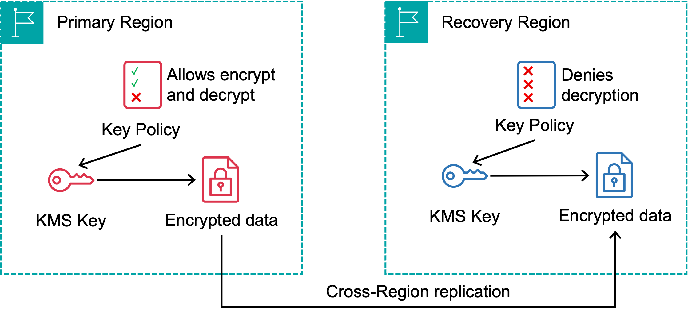
Figure 1 – Server-side encryption architecture using AWS KMS with cross-Region replication.
You can also use this approach with client-side encryption for backups you manage and store in S3. Customers manage their own backup processes and use the
AWS Encryption SDK or their own clients with
multi-Region AWS KMS keys to encrypt the data. Multi-Region keys allow you to encrypt and decrypt replicated S3 data in multiple Regions using the same key material.
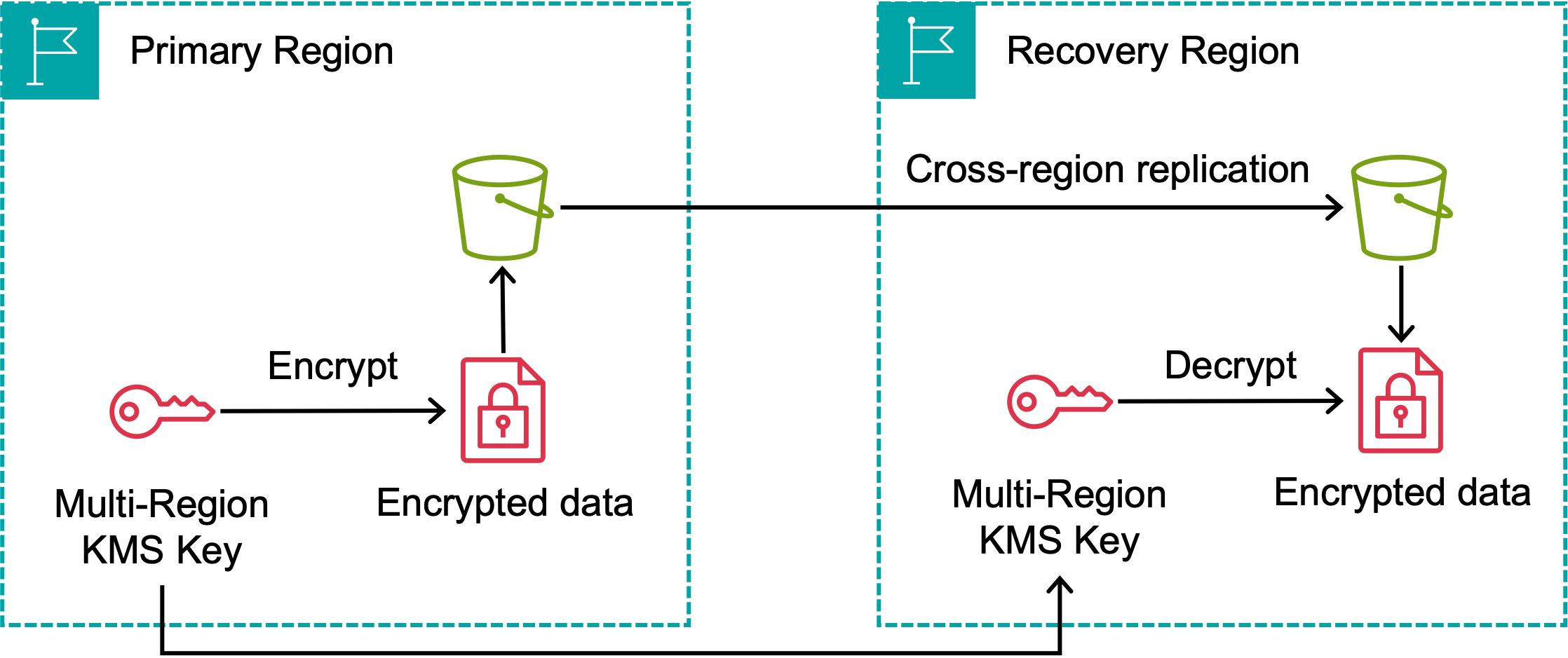
Figure 2 – Client-side encryption approach using multi-Region AWS KMS keys.
You can explore additional strategies for enhancing controls on the key policies to meet your requirements. For example, you can require Multi-Factor Authentication (MFA) to update your key policies. This allows the MFA holder and credential holder to be two distinct parties. They could be two different teams within an organization, or you could consider greater separation by providing the MFA device to a trusted third party such as a regulator. Another option is to implement controls in your identity provider to issue specific IAM session tags that provide conditional access to update the key policy. You should also scope key policy update permissions to a set of named IAM principals using condition keys, so that only explicitly authorized identities can modify decryption access.
Choose this strategy when storing encrypted data in a partner country is acceptable. Key policies prevent unauthorized access, and this approach offers the simplest operational model with the lowest recovery time.
Strategy 2: Data boundary
In this strategy, you store backups or operate a pilot light recovery environment on AWS Outposts in an on-premises site within the source country or other approved location. You replicate data from your primary Region using tools such as AWS DataSync for S3 data or other replication tools like MySQL binlog or Postgres logical replication for Amazon Relational Database Service (Amazon RDS) instances. You maintain full control of where your business data physically resides at all times. You can also use third-party backup solutions to replicate data from your primary Region to on-premises or in-country storage.
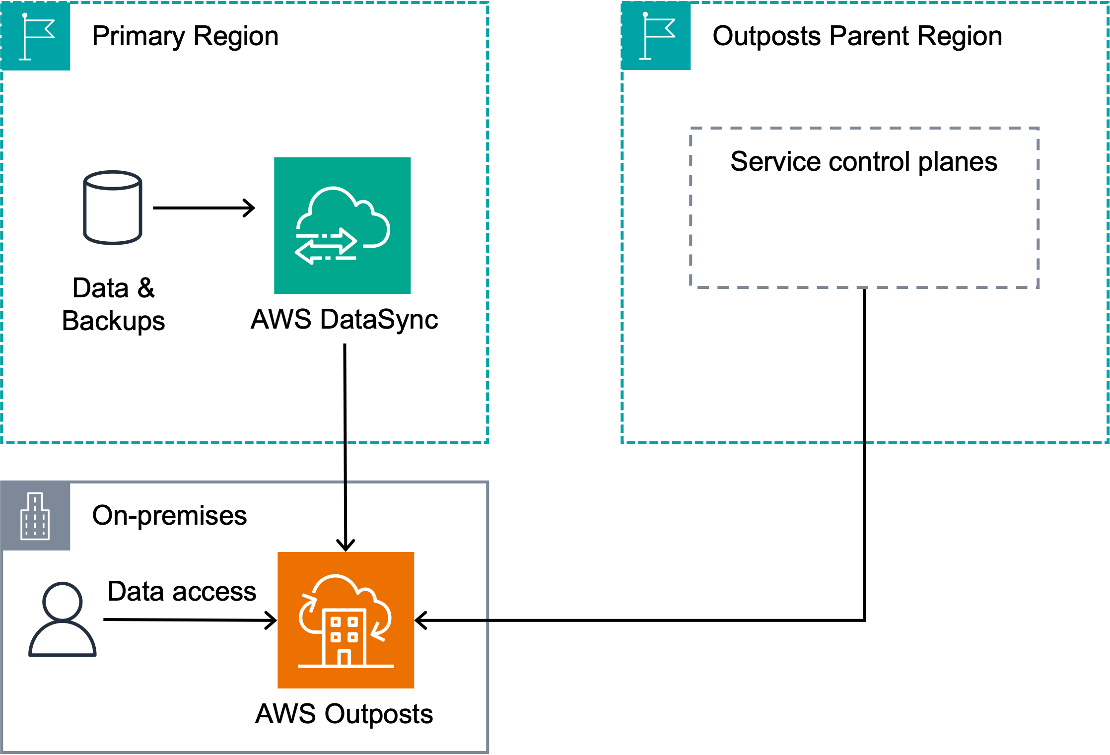
Figure 3 – AWS Outposts recovery architecture with data replicated to on-premises infrastructure.
Data access occurs directly over the local network in your on-premises facility through the
data planes of the resources hosted on the Outposts infrastructure. These are resources like
Amazon Elastic Compute Cloud (Amazon EC2) instances, Amazon RDS database instances, and S3 buckets. You provision and configure those resources through each service’s
control plane, which is hosted in the parent Region you select when you order your Outposts racks.
Choose a parent Region that is different from your primary Region. This prevents simultaneous impact to your primary workloads and your ability to use control plane operations for recovery, such as launching new instances on your Outposts. Note that Outposts are not designed for disconnected operations or environments with limited to no connectivity. Maintain highly available networking connections from your on-premises site back to the parent AWS Region.
During recovery, you can restore your environment directly on the Outposts infrastructure. AWS Outposts support a subset of the available AWS services in a Region, so you need to design your workloads to use the services available. Alternatively, you may obtain regulator agreement to restore your environment from backups stored on your Outposts to an AWS Region in a different country during extreme circumstances.
Select this strategy when you must physically maintain your backups and data in specific locations, want a consistent experience using AWS services and hardware in the cloud and on-premises, and using control planes for your Outposts infrastructure from outside your primary Region is acceptable.
Strategy 3: Strict local autonomy boundary
Some data residency frameworks, such as those in financial services or national security contexts, may require customer data and the control plane systems used to manage that data and recovery environments remain within national borders. Two options achieve this outcome.
Option 1: On-premises infrastructure
In this option, you operate hardware and software in an on-premises location to store backup data. Like the Outposts option, this provides flexibility on where backed-up data is restored: it could be restored to on-premises physical hardware or to an AWS Region in a different country.

Figure 4 – On-premises backup architecture with data copied from Amazon S3 to local storage.
This solution requires you to self-manage backups in S3, then copy them to on-premises storage using tools like AWS DataSync. You need to decide how to manage encryption of your data on-premises. Encrypting and decrypting data on-premises should not depend on the availability of the primary Region.
Option 2: Multi-cloud
In a multi-cloud solution, you can replicate backups from your primary cloud to an environment on another cloud provider and recover your workloads there. You can also use a lifeboat strategy.
A lifeboat strategy involves running a separate set of systems in another cloud provider which meets your residency requirements. These systems are not replicas of the primary platform. They are built and developed natively to provide a subset of critical functionality. This approach avoids architecting to the least common denominator of services across providers. You can take full advantage of all services available on AWS for your primary workload while the stand-in system uses a separate, purpose-built architecture.

Figure 5 – Multi-cloud lifeboat architecture with a purpose-built stand-in system.
Monzo Bank’s stand-in system is a well-documented example of this pattern. Monzo operates its primary banking system on AWS with thousands of microservices. Rather than replicating that entire stack, they built a small set of purpose-built services on a separate cloud provider that supports only the operations most critical to their customer experience: card payments, bank transfers, and balance information. According to Monzo, the stand-in shares no code and no infrastructure with the primary system.
The lifeboat pattern follows several key design principles. The stand-in supports only key functionality, which helps minimize the cost of the solution. Using different software reduces the probability that the same defect or failure mode affects both systems simultaneously. The stand-in accepts eventually consistent data, which avoids strong coupling between the two environments and preserves availability independence. The recovery does not appear transparent to end users. The experience is intentionally degraded to a subset of services, which is an explicit trade-off for maintaining availability.
A multi-cloud lifeboat provides protection against service disruptions of an AWS Region in a single country, but using multi-cloud to keep data in-country may not fully mitigate scenarios where all major cloud providers in a geography face simultaneous disruption.
Testing
You must continuously test your recovery strategy to build and maintain confidence it will succeed during a real event. Testing must be performed end-to-end: validating the integrity and consistency of backups, launching compute and database resources, and running synthetic test traffic through the recovered system. The more frequently you test, the more recovery becomes a standard operational process rather than a one-off monthly or quarterly activity. Your testing must keep up with the rate of change in your environment. If a change breaks your recovery process, you want to know about it and fix the procedures as quickly as possible.
The approach to testing is generally the same as traditional multi-Region recovery testing, but the additional complexities and operational processes of these solutions require an increased level of rigor:
- Strategy 1 (Cryptographic boundary): You need to decide if decrypting data and launching recovery environments with that data is acceptable. Ideally, you run full end-to-end recovery tests during approved test windows. If you cannot, you need to test your recovery procedures using synthetic data that is not subject to data residency requirements. This helps validate your recovery procedures, but it does not prove you can recover your critical business data.
- Strategy 2 (Data boundary): Validate replication lag meets your recovery requirements. Test launching recovery workloads on Outposts infrastructure and confirm that the parent Region control plane can orchestrate recovery while the primary Region is simulated as unavailable.
- Strategy 3 (Strict local autonomy boundary): For on-premises recovery, validate that backups can be restored to your target environment and that workloads function correctly outside of AWS. For multi-cloud lifeboats, test failover activation and verify that the lifeboat has no dependencies on your primary environment.
Summary
In this post, we presented three strategies for implementing disaster recovery solutions that support data residency requirements:
- Strategy 1 (Cryptographic boundary) uses encryption to meet the intent of data residency while using multi-Region AWS infrastructure for recovery. This offers the lowest operational complexity and best recovery performance, if permitted by applicable regulations.
- Strategy 2 (Data boundary) uses AWS Outposts to maintain data in-country in customer-controlled facilities while using an out-of-country control plane for management operations, if permitted by applicable regulations.
- Strategy 3 (Strict local autonomy boundary) keeps both data and control in-country during a recovery event using on-premises infrastructure or a multi-cloud lifeboat strategy. This offers the highest degree of control but with the greatest operational complexity.
The option that works best will be a joint decision between your business, regulators, and your customers. You should consider potential failures proactively and build recovery plans before an event occurs. This framework provides a structured way to evaluate the trade-offs and determine where to invest based on your regulatory environment, risk appetite, and operational capabilities.
Next steps
To learn more about the services and approaches discussed in this post, see the following resources:
- Disaster Recovery of Workloads on AWS
- AWS Key Management Service
- AWS Outposts
- AWS Backup
- AWS DataSync
If you have questions about applying these strategies to your specific workloads and regulatory environment, reach out to your AWS account team to discuss your recovery requirements in detail.
About the authors
The DOJ’s Firings & Hirings #lastweektonight
Post Syndicated from LastWeekTonight original https://www.youtube.com/shorts/Aox7kVRQl-c
rsync 3.5.0 released
Post Syndicated from jzb original https://lwn.net/Articles/1088759/
Version
3.5.0 of rsync has been released with a huge
number of security fixes:
This release fixes 33 security issues found during a focused audit of
rsync’s path handling and daemon protocol, a companion daemon-protocol
fuzzing pass, and reports from external researchers -- plus several
robustness hardenings. CVE IDs were assigned by VulnCheck (CNA); the
precise “introduced in” version ranges accompany each advisory, and
many are much narrower than “everything before 3.5.0”. Every fix ships
with a regression test in the test suite that fails on the unfixed
tree.
[$] 128-Bit page tables for Arm
Post Syndicated from corbet original https://lwn.net/Articles/1088125/
The size of a processor’s page-table entries directly limits how much
physical memory that processor is able to access. Back in the 32-bit days,
that limit was 4GB, an amount of memory that once seemed nearly infinite,
but which would now struggle to hold a basic AI-enabled “hello world” app.
The expansion to 64 bits on most popular architectures would seem to
have removed those limits now; some Arm systems, for example, can use
56 of those bits to access up to 72PB of memory. So it might be
surprising that the Arm architecture is evolving to support even larger
page-table entries (PTEs). This
patch set from Anshuman Khandual adds support for 128-bit PTEs, but
who will benefit from this capability is not entirely clear.
Незаконните билбордове, рекламата на хазарт и визуалното замърсяване в София
Post Syndicated from Боян Юруков original https://yurukov.net/blog/2026/bilboards-sofia/

Преди две седмици писах как за кратка отсечка в София преброих 28 билборда. Повечето рекламираха хазарт, което е забранено по закон. Закон, който изглежда никой не спазва и никой не налага. Както доста други преди мен се запитах как е възможно това. НАП са се извинявали в миналото, че тия не били баш реклама на хазарт, а и не знаели къде и колко са всъщност билбордовете. Затова реших да отговоря на този въпрос. Като за начало за София.
За целта свалих данните на Столична община за билбордовете от слой на iSofMap. Там открих 468 билборда на общинска земя по предварителна схема приета от Столичен общински съвет преди доста години. Заедно с тях са отбелязани 976 билборда на частна земя. Забелязах, че много рекламни пространства, които виждам, ги няма на тази карта и добавих данните от GovAlert за всички разрешения за поставяне, в които се споменава „реклама“ под някаква форма. Това добави още 1355 записа към данните.
Така получих 1917 точки на картата. Подробности как съм ги обработил и методологията ще прочетете след малко, но същественото е, че минавайки из града в последната седмица виждах билбордове на всяка от отбелязаните точки. Изключенията бяха единици, но за сметка на това виждах доста рекламни пана, които не бяха на картата. Ярък пример е установената за незаконна видео рекламна стена на Тиков на 4-ти км.
Но от данните видях нещо също толкова притеснително – над една трета от билбордовете и рекламите по сгради в София са с изтекли разрешителни и няма данни да са продължавани. Някои са изтекли в последните три месеца, други – преди години. Още 59 изтичат до края на годината. Отделно повечето от онези по общинска схема или 27% от всички са изтекли или ще изтекат скоро, а не изглежда да има дискусия или план какво да се прави с тях.
Затова нека се вгледаме по-подробно в данните, какво знаем, какви са известните проблеми и какво е неизвестно по темата.
Източници и методология
Както споменах по-горе, основните данни идват от картата за реклами и преместваеми обекти на Столична община. Изключвам от там схемите за поставяне на маси. Разрешителните за ползване взех от регистъра на НАГ като ги свързвам с поземления имот през алгоритъма на GovAlert. Ще ги намерите също на картата с документите от градоустройството. От тях взимам само тези споменаващи реклама в описанието.
Данните от iSofMap имат няколко особености и проблеми. Първо, няма много информация за схемите на билбордове на общински парцели. В доста от записите липсва и последната цифра на разрешението и затова ще видите въпросителна в картата ми. Повечето са обаче на около 10 години. Доколкото разбирам, много от договорите са изтекли, но са оставени в сила, докато не истекат останали и се реши какво да се прави за всички пространства.
За рекламите на частни парцели знаем повече. Вторият проблем е, че много разрешителни налични в НАГ липсват на картата, както и много рекламни пространства. Точките на тази карта показват конкретните елементи като някои са с общо разрешение за поставяне. Обединявам ги на картата само, когато географските координати са еднакви, т.е. са практически един до друг.
По номера на разрешителните свързах повечето от тях с регистъра на НАГ, т.е. може да достъпите самия документ. За 68 от тях или 8.1% разрешителното не е публично. Всъщност, става въпрос за 46 разрешителни, защото няколко от тях са за повече обекти. От тях 18 би следвало да са още валидни. Всеки служител издаващ такива документи е длъжен да го публикува в регистъра, т.е. говорим за пропуски или умисъл. Не са дори стари разрешения – някои са от 2012, но има и такива, които все още са валидни от 2023 и 2024 и също липсват. Липсващи документи в регистрите на НАГ не са изключения обаче и особено такива за поставяния съм засичал неколкократно да се укриват, особено покрай обекти на Национална спортна база в Изгрев.
Тук е важно да се спомене и срокът за валидност на разрешенията. Докато при общинските схеми за поставяне е доста мътно какво се случва, тези на частни земи се издават със срок от пет години. Този е намален от 10 години с решение в средата на 2018-та и влиза сила през септември същата година. Т.е. би следвало разрешения за поставяне издадени преди септември да са с 10 годишен срок. Например, разрешението за светещия надпис на Артекс над първия Диамант е издадено през юли 2018 и важи още две години, освен, ако живеещите в сградата не решат да прекратят договора за надписа, по който би следвало да получават наем. Подалите след септември следва да са с 5 годишен срок.
Практиката е друга. Първо, че за смятане на кой режим се използва е взета не датата на заповедта или обсъждането в комисия, а датата на подаване на заявлението. Един пример тук е покривна реклама над сградата на Джъмбо на бул. България. Има обаче няколко случая, в които тогавашния главен архитект Здравков е налагал двоен стандарт. Някои подадени през август са получили 5 години срок, а други като надпис на Harmony Group на офис сграда на бул. Черни връх има срок от 10 г. независимо, че молбата е подадена през октомври. Заради тези противоречия прегледа всички разрешителни издадени през 2018 и 2019-та и отбелязах какъв е реалният срок. Някои са издавани с 10 годишен срок чак през март 2029-та.
По номерата на разрешителните свързах линковете в регистъра с точките от картата с преместваемите обекти от iSofMap. Както спомена горе, за някои разрешения има отбелязани повече точки, тъй като са позволени повече рекламни обекти. Така 721 разрешения бяха свързани с 839 точки на частни имоти. Когато обаче подобно свързване не беше възможно в 610 разрешителни, не можех да отбележа точното местоположение на рекламата. Затова ги сложих в центъра на парцела и при натискането му се показва цялата зона, където би могъл да бъде. Докато някои парцели са малки, други са значителни и имат по няколко билборда. Това има страничен ефект, че една точка може да разрешава няколко билборда пръснати из голям имот, а на картата да стоят като една точка. Това произтича от липсата на актуални данни в НАГ.
Друг проблем е, че някои билбордове и други рекламни елементи имат няколко поредни разрешителни, някои изтекли, а други – не. В данните на iSofMap те са като отделни точки с няколко метра разстояние. По контекста се разбира, че става дума за същото място или същия обект. В други случаи това не е ясно. Когато такива точки са много близки, ги свързвам и показвам списък на разрешения за това място. Ако последното като хронология е още валидно, отбелязвам точката като валидна. В други случаи обаче има само изтекло разрешение в данните на рекламните елементи и откривам ново в регистъра с разрешенията. При вторите знам само парцела, а не точното място. Независимо, че бих могъл да ги свържа, ако в този парцел има само един рекламен елемент, това предразполага към грешки. Затова е възможно на места на картата да видите близко един до друг изтекъл билборд и до него в същия парцел нов валиден такъв. Макар да са доста малко тези случаи и бих могъл да ги разгледам един по един, не искам да правя предположения по заглавията и имената на фирмите и представих данните във вида и с качеството както са на страницата на общината.
Не на последно място, категоризирах някои от валидните разрешителни според това дали са билбордове или реклами върху сгради или на стени. Направих това отново по ключови думи и сложих филтри в легендата. Макар някои от тях да са реално фирмени надписи, това отново е реклама, която допринася до визуалното замърсяване на града, особено предвид, че повечето светят нощем.
Може да свалите таблиците с изходните данни за схемите за поставяне на общинска земя, елементи и разрешителни. Включил съм координатите и номерата на поземлените имоти.
Карта и сигнали
Поставих всички точки на карта аналогична на тези, които съм правил с подобни визуализации. От бутоните вляво може да смените базовия слой със сателитна карта на София и да фокусирате картата върху местоположението си. От легендата може да изключвате от картата различни категории реклами и разрешения.
При натискане на някоя точка се отваря известната за това място информация. Ако е само разрешение, на картата ще се покаже и района на поземления имот, където вероятно все още е билборда или рекламния обект. Ако виждате нарушение, може да натиснете на линк с указания как да подадете сигнал.
Тук може да разгледате картата, както и да я отворите на цял екран за по-удобно.
За разлика от другите проекти на отваряне на данни, този има заглавна страница представяща нещата различно. Тя започва с два бутона. Единият води към картата, а другият използва същите данни и местоположението на посетителя (ако разреши достъп до такова), за да установи най-близките рекламни пространства и дали са валидни. Показва ги в списък и натискане на някой от тях представя същите подробности и линк към документа, ако такъв е известен.
Под списъка и подробностите има указания как да се подаде сигнал към Столична община през системата Call.Sofia. С обновлението ѝ, линкът позволява предварително въвеждане на категория и подкатегория. Остава да се избере точно място, да се отговори на въпрос, че става въпрос за „Извършване на нерегламентирана рекламна дейност“ и да се попълни заглавие и описание. Съветвам да се добавя тага #noads, за да намирам по-лесно сигналите и да мога да ги покажа на картата. Важно е да се добави и снимка, на която се вижда улицата и съседните сгради, за да може ясно да се идентифицира за кой точно билборд става дума. Както сами сте свидетели има места из града с до 20 такива наоколо, което както затруднява свързването на сигнала с конкретен обект, така и още веднъж показва колко са излезли нещата извън контрол.
Трябва да подаваме сигнали, за да се установи дали тези обекти имат разрешения, дали са валидни въобще, но също и дали обектът отговаря на разрешението. Примерите в следващата секция показват, че намираме валидно понякога разрешение за малък едностранен билборд, а на място се вижда значително по-голям такъв. Ако отговорят, че има разрешение за поставяне, следва въпросът защо не е публично, както е нормативното изискване в общината и защо не присъства на картата с рекламите в София.
Оперативни и нормативни проблеми
Обществена тайна е, че много от рекламните площи са незаконни, с изтекли разрешения или че такива въобще не е трябвало да бъдат издавани. Системният контрол над тези и други преместваеми обекти е труден и както сам съм свидетел редовно, не се случва дори при подадени сигнали. Пример за това са проблемите със задължителното озеленяване на жилищни комплекси и строителство без разрешение от НСБ в Изгрев. Дори причината да се вгледам в тази тема – видеостената на хотела на 4-ти км. – беше установена като незаконна едва след множество сигнали от района. Въпреки това все още си е там докато сигналът пътува между офисите из НАГ. В този смисъл, за този портал, данните и евентуалните сигнали произтичащи от тях може да благодарим на Тиков.
Не трябва да гледаме далеч от този казус обаче, за да видим други проблеми. В рамките на кръговото на 4-ти км. се забелязват 15 билборда и една реклама на комин. На картата ги виждаме всички плюс няколко надписа на сгради. Поне три от тях са с изтекли разрешителни, а две от тях заедно с още едно с валидно разрешително до март 2028-ма са за едностранни билбордове. На снимките виждате последните три, които имат реклами от две или три страни.



В центъра на кръговото виждаме шест билборда по схеми за поставяне от общината заедно с още поне два малко извън кръговото. Всички са на общинска земя и в зелени площи. По наредба за ремонт и смяна на рекламите може да влизат и паркират тежки коли в зелените площи, както и да се изсичат дървета и друга зеленина, за да са видими тези и други реклами. Освен визуалното замърсяване, всичко това допринася и много до унищожаването на зелени площи. Тук не говорим само шест билборда, а стотици, които всеки месец налагат подобни действия на подобни места.
Следващите два примера пък показват как точките от картата с рекламите на общината се групират. В случая става въпрос за билбордовете по периметъра на мол СкайСити. Разрешението е за общо 19 такива пространства. Точките от данните на общината са 9 като няколко от тях събират по 2 или 3 билборда. Разрешителното за всички тях са изтекли преди три години след като са имали 10 години срок на действие.

Тук се сблъскваме с няколко проблема. Първо, както обсъдих преди не е ясно дали и колко от тези рекламни пространства имат нови разрешения за ползване, които по някаква причина не са станали публични. За онези 46 неизвестни попитах НАГ с номерата, за да се разбере дали е техническа грешка, не съществуват или е друго. Тук още по-ярко се вижда липсата на единния регистър по ЗУТ, който все още очаква подписа под наредба на кабинета на Радев. Писах за това покрай случая в Баба Алино. Този регистър следва да помести не само тези разрешения за поставяне, но и всички в цялата страна с ясна проследимост.
Лошото качество на данните личи най-вече в слоя с рекламите и преместваемите обекти, където много нови билбордове с валидни разрешителни липсват, а изтекли такива изглежда все още стоят. Не може да разчитаме на него като източник на реалното състояние в София и затова призовавам всички да се огледат и да подават сигнали.
Оперативно изглежда няма достатъчно проверки или поне резултат от тях. Възможно да е въпрос на капацитет или желание. Доколкото получих отговори, тази задача се пада на Столичен инспекторат, който следва да следи за изпълнението на задълженията по тези договори и разрешения. Възможно е да не са само те. Възможно е да страдат от същият недостиг на качествени данни кое е законно и кое не, с който се сблъсках аз. Фактите са обаче, че при редица сигнали дори за елементарни бутки и бариери или сеч на дървета, районно кметство, който единствен отговаря за издаване на такива разрешителни, пита установения извършител да предостави документ. Т.е. не си вярват на собствената деловодна система или не си спомнят какво са подписали и за кого. Вероятно е било на крак, вероятно нарочно не е входирано дигитално и направено публично. Надявам се да е просто тяхното разбиране за процеса, а не тупат топката докато всички забравят, за да не се налага да пишат акт. Такива случаи имам наскоро по сигнали за отрязани дървета в Младост и преместваеми обекти в Изгрев.
Лошата проследимост до сега, липсата на документи, отчетност и отговорност скриваше подобни случаи. Получих уверения, че новата система на Call.Sofia ще поправи това и следва да го тестваме. Трябва обаче да се вдигнем очи и да се огледаме и вместо да се ядосваме защо има повсеместни реклами на хазарт и следващото уж зелено бетонно туловище, да се запитаме защо въобще е бодната тази реклама там и не само дали е законна, а следва ли да е там въобще.
Тук стигаме до нормативните проблеми. И сега има законов път, по който да се получи разрешение за такива реклами. Този процес обаче от една страна е утежнен процедурно – комисия в НАГ за схемата и после отделно молба за поставяне. От друга времето за такова разрешение силно варира и е значителен източник на корупция. Както стана видно от решенията по времето на Здравков, срокът е даван както дойде. Тогава някои решения са били получавани месец след искане, а други – година и половина. Срокът трябва да е в седмици и да може да се продължи разрешение в рамките на шест месеца преди да изтече старото. Реалността обаче е, че за някои от тези билбордове, за които ще подадем сигнали, има молба за разрешение, която престоява с години, а обектът още си стои с погрешен претекст, че има производство по случая. Нищо, че вероятно не може да получат разрешение по принцип.
По принцип има редица ограничения, но далеч не са достатъчни, за да не се претоварва града с 1500 билборда закачени къде ли не. Скоро ще тръгне отново темата за тези общинските билбордове, но те са само малка част от всички. Липсва стандарт, който да се следва. Може да е визуален или метрика на площ. Разумно би било да се намалят рекламните площи най-малкото три пъти. Ако приложим стандартите на други големи европейски градове, както много обичат да правят общински съветници и архитекти, следва да забраним изцяло рекламата на покриви и стени на сгради и да има не повече от 100 билборда в града по булевардите.
Какво следва да се случи?

Първото нещо е да покажем колко масов е проблемът с незаконните реклами подавайки сигнали. Описал съм в проекта как може да стане това.
Второто е, че трябва да решим как искаме да изглежда градът ни – описан с билбордове и реклами по покриви или изчистена градска среда. Тук едни ще кажат, че това носи доходи на общината, а частни лица следва да могат да правят каквото си искат с имотите си. В действителност никой имот не е в изолация в града и трябва да се съобразява с останалите, а доходите за общината може да се компенсират с по-малки и незатормозяващи рекламни пространства. Тук следва да решим какви следва да са тези правила и да изискаме от Столичния общински съвет да ги наложи.
Трето, следва да следим пътят на сигналите, позициите на местните избраници, предложенията и дискусиите им. Често последните минават набързо и на тъмно защото обществото така и не разбира, че е тема в дневния ред или че това, което се готви ги засяга пряко.
Четвърто, започнах с темата за хазарта с причина. Рекламите на хазарт са основен двигател на всичко, което описвам и много от билбордовете са собственост именно на фирми свързани с хазартния бизнес. Докато рекламата на хазарт не бъде повсеместно забранена независимо къде се намира, няма да има решение този проблем. Заедно с бързите кредити и телефонните измамници, хазартът носи най-големи негативи за благосъстоянието на българското общество и особено най-уязвимите от него. Намирам за изключително цинично да се обсъждат акцизи и печалби за местна и централна власт в този контекст. Не по-малко цинично и опитите за триене на имиджа им чрез финансиране на спортни отбори и зали. Ако приемем всички тези като каквито са – просто реклама на хазарт и разпознаем щетата, която има върху обществото ни, то дори това би бил достатъчен повод да преразгледаме основно броя и разположението на рекламните площи в града.
Не на последно място, трябва да направим крачка назад и да разберем, че градската среда не е просто красива картинка, която виждаме само по рекламите на жилищни сгради, а съвкупност от планиране, изпълнение и контрол. Тук засягаме планирането и контрола по един елемент от нея – рекламите. Освен него има замърсяване на въздуха, водата, почвата, с шум и светлина, които влияят пряко на качеството на живота и здравето ни. Тук фактори са достъпността на средата, обществения транспорт, качеството на строителството и спазването на стандартите и прочие. Важен фактор е и озеленяването, темата за която ще засегна нашироко скоро. Не може да отмятаме с лека ръка който и да е от тези компоненти смятайки, че не е най-големият проблем. Това се случва всъщност с всеки един от тях един по един и накрая се чудим защо градовете ни изглеждат толкова зле.
Осъзнаването на проблема е важна стъпка, но често спираме там. Този път молбата ми е да направим следващите две крачки и да подаваме сигнали, да следим изпълнението им, да изискваме отговори резултат. Може би ще даде полезен пример за другите елементи на градската среда и модел за засягането на проблемите там.
Security updates for Thursday
Post Syndicated from jzb original https://lwn.net/Articles/1088715/
Security updates have been issued by AlmaLinux (abrt, dhcpcd, edk2, freerdp, gegl04, grafana, gstreamer1-plugins-good, iscsi-initiator-utils, isns-utils, kernel, kernel-rt, keylime, libarchive, libyang, nodejs-nodemon, opencryptoki, osbuild-composer, pacemaker, postgresql-jdbc, postgresql18, python-idna, python3.9, udisks2, valkey, vim, xorg-x11-server-Xwayland, and yggdrasil-worker-package-manager), Debian (flatpak, lemonldap-ng, neutron, python-django, spip, xdg-dbus-proxy, and xorg-server), Fedora (apr-util, cri-o1.34, libcupsfilters, linux-firmware, sqlite, and vaultwarden), Gentoo (FreeType), Oracle (dovecot, evince, fence-agents, gnutls, gstreamer1-plugins-bad-free, gstreamer1-plugins-good, isns-utils, java-1.8.0-openjdk, kernel, libarchive, osbuild-composer, pipewire, postgresql, ruby, ruby:3.3, sudo, and udisks2), Red Hat (bind, bind9.16, gnome-remote-desktop, grafana, opentelemetry-collector, python-pillow, python3, python3.12, python3.14, python3.9, and rhc), SUSE (chromium, clusterctl, dracut, gd, git-cliff, gleam, govulncheck-vulndb, graphicsmagick, gzip, kernel, kubevirt, libheif, librest0_7, nodejs22, nodejs24, openssh, openvpn, python3, python313-scikit-learn, rpm, stunnel, and zk), and Ubuntu (kernel, libgit2, linux, linux-aws, linux-aws-fips, linux-azure, linux-azure-6.8,
linux-azure-fde, linux-azure-fde-6.8, linux-azure-fips, linux-fips,
linux-gcp, linux-gcp-6.8, linux-gcp-fips, linux-gke, linux-gkeop,
linux-ibm, linux-ibm-6.8, linux-nvidia, linux-nvidia-6.8,
linux-nvidia-lowlatency, linux-realtime, linux-realtime-6.8, linux-xilinx, linux, linux-aws, linux-aws-fips, linux-azure, linux-azure-fde,
linux-azure-fips, linux-gkeop, linux-ibm, linux-ibm-5.15,
linux-intel-iot-realtime, linux-intel-iotg, linux-intel-iotg-5.15,
linux-kvm, linux-nvidia, linux-nvidia-tegra, linux-nvidia-tegra-5.15,
linux-oracle-5.15, linux-realtime, linux-xilinx-zynqmp, linux, linux-aws, linux-aws-fips, linux-azure-4.15, linux-azure-fips,
linux-fips, linux-gcp-4.15, linux-gcp-fips, linux-kvm, linux, linux-aws, linux-azure, linux-azure-fde, linux-ibm, linux-oracle,
linux-raspi, linux-realtime, linux-azure, linux-azure-6.17, linux-gcp-6.17, linux-hwe-6.17, linux-oem-6.17,
linux-realtime-6.17, node-follow-redirects, and yelp).
Certificate Transparency Monitoring is now generally available
Post Syndicated from Pravallika Nakarikanti original https://blog.cloudflare.com/certificate-transparency-monitoring-ga/
Since we launched Certificate Transparency Monitoring in public beta in 2019, we've been emailing subscribers whenever a new TLS certificate appears in a public Certificate Transparency (CT) log for one of their domains. Today, it's turned on for more than 650,000 customer domains. It's an early warning that someone, somewhere, has issued a certificate for a hostname in your zone, giving you a chance to spot a mis-issued certificate early.
It's a useful signal, but it had a noise problem, and we felt it ourselves. Cloudflare issues a large volume of certificates on your behalf: Universal SSL renewals, certificates from Advanced Certificate Manager, and backup certificates. All of them are logged to public CT logs by design, because a certificate that isn't logged won't be trusted by major browsers like Google Chrome and Apple's Safari. So the same transparency that lets you monitor for mis-issuance also surfaces every certificate we issue for you.
And issuance isn't a one-time event. Certificates are short-lived and renew automatically: a single Universal SSL certificate can renew as often as every 60 days, up to about six times a year. That cadence is set to increase, with the CA/Browser Forum having voted to cut the maximum certificate lifetime to 47 days by 2029, multiplying the routine renewals that flow through those logs. Every one of those renewals generated an alert. But at the scale Cloudflare issues certificates, a genuinely suspicious one could look just like a routine renewal, and the alert that mattered was easy to miss.
We heard the same thing from customers. On our community forum, one described disabling the feature across all their sites because they were "tired of regularly getting spammed with tons of completely normal certificate renewals," adding "I wasn't even actually reading them by the end." That noise came from Cloudflare's own certificates.
Today, we're changing that. Certificate Transparency Monitoring now filters out the certificates Cloudflare issued on your behalf before an alert is sent. The alerts that reach your inbox are the ones that deserve your attention: a certificate you didn't expect, that Cloudflare didn't issue. With that fix in place, Certificate Transparency Monitoring is generally available.
Filter out the certificates Cloudflare manages
The goal is to identify and eliminate noisy alerts for routine, Cloudflare-managed certificate issuances and renewals while ensuring we catch all external certificates managed outside our system.
Why couldn't we just identify and filter these out previously?
There are two independent systems built to serve separate products: certificate management, which deals with internal certificate issuance data, and CT alerting service, which parses data from public CT logs.
The two flows handle the same certificate, but never at the same moment and never with the same information. When the alerting flow is deciding whether to email you, all it has is what it pulled from the log. It has no signal from the issuance flow saying "the ordering service just created this one." That missing link was the problem.
What is the lifecycle of a certificate?
As shown above, certificate issuance happens in two stages:
- Certificate Authority (CA) creates a pre-certificate, writes to logs and receives SCTs (Signed Certificate Timestamps).
- CA embeds those SCTs into the final certificate and logs it.
Thus, the alerting service sees two log entries for a single certificate order: 1) pre-certificate and 2) final certificate. To avoid alerting twice per pair, an internal identifier called stripped_fingerprint is stored for deduplication purposes. This fingerprint is the hashed value of DER (Distinguished Encoding Rules)-encoded TBSCertificate (to be signed certificate). This value is consistent and unique for a pre-certificate/final certificate pair that belongs to the same certificate order. Therefore, this is one identifier which is already present, and it sits entirely inside the alerting flow.
Why does the obvious fix fail?
The intuitive shortcut is to copy stripped_fingerprint into the ordering service so the alerter can look it up. But that doesn't work because the ordering service doesn’t receive the pre-certificate, so it can't produce this value when the alerting service receives it.
So even if this is used as an identifier, it can only be recorded after the final certificate is received by the ordering service. In that window between pre-cert and final cert log entries, if the alerting service looks up stripped_fingerprint(precert) in the ordering service’s database, then it is not going to find any information matching this identifier to confirm that it is issued by us — and this leads to an extra alert again.
Although the certificate ordering service is the right system to answer “Is this ours?”, the match key with which this information was being uniquely identified is not winning the race. So the problem reframed itself. The question was no longer where to store the fingerprint, but what is that one identifier which can be persisted from order creation to the final logged certificate.
What is the right key?
The right key had to check these boxes:
- Early: recorded before anything reaches the log, i.e., present at key generation.
- Consistent: throughout all stages from pre-certificate to final certificate.
- Reproducible: the CT alerting service can recompute it independently, from the log entries alone.
- Unique: to each certificate order.
The public key is one such identifier that checks all those boxes. It travels inside a structure called SubjectPublicKeyInfo (SPKI).
Consistency: As the diagram above shows, SubjectPublicKeyInfo (SPKI) is present from the first step and stays the same through the CSR (Certificate Signing Request), pre-certificate, and final certificate.
Uniqueness and Safety: Cloudflare generates a fresh keypair for every issuance, so the public key is effectively unique. Since only Cloudflare has the private key, a certificate with a matching SPKI must have come from a Cloudflare issuance only. A collision is astronomically unlikely, and no outsider could create a valid signing request without the private key.
So the identifier we record is spki_sha256 — an SHA-256 hash of the DER-encoded SPKI, a short fixed-length value that's cheap to index. The ordering service computes it straight off the CSR and writes it at key generation, before issuance begins.
How do both flows agree on the value?
Recording the key early solves this in the certificate ordering. With that in place, the alerting flow performs an extra step. When the alerter sees a log entry, it recomputes spki_sha256 from the certificate's public key and looks it up to see if the ordering service has recorded this value in its database – on:
- Match → the ordering service recorded this key, so the certificate is ours. Suppress the alert.
- No match → key not found – alert, exactly as before.
Because the key is identical in the pre-certificate and the final certificate, it no longer matters which one arrives first.
Three things follow, all toward less noise:
- Certificates we manage no longer alert you. Universal SSL, Advanced Certificate Manager, Total TLS, and Backup Certificates all match a recorded key and pass silently.
- Abandoned pre-certificates no longer alert you. Sometimes a pre-certificate is logged but issuance never completes. Those alerts used to look like unexplained certificates; now they match a record and stay quiet. The event is still recorded on our side; we just don't email you about something we already know is ours.
- Custom certificates you upload still alert you. We didn't generate those keys, so there's no record on the issuance side and nothing to suppress. That's exactly the case CT monitoring and alerting exists for, and it's untouched.
Most of the work here wasn't writing the fix; it was understanding both flows well enough to see that the key connecting them was a field we'd been carrying the whole time. Once we picked the identifier that's early and shared, the rest was bookkeeping.
CT alerting should fire only on issuance we can't account for. With this change, it does.
Alerts are now easier to review
Updated emails identify the affected hostname in the subject line, include certificate details in the message, and link to the certificate in the Cloudflare dashboard, so you can review it and take action as needed.
What's next
We plan to bring Certificate Transparency Monitoring to Cloudflare Notifications. This would let teams route CT alerts to webhooks, PagerDuty, or additional email destinations, just as they manage other Cloudflare alerts, instead of relying on today’s email-only channel.
Try it
Already using Certificate Transparency Monitoring? There is nothing you need to do. Filtering is already enabled. Starting today, you will only be notified of certificates issued outside of Cloudflare's automated systems.
Not using it yet? In the Cloudflare dashboard, go to SSL/TLS → Edge Certificates → Certificate Transparency Monitoring and turn it on. Available on every plan at no extra cost, with unified settings across plan tiers, so you can manage alert recipients in one consistent view.
If you have thoughts on how Certificate Transparency Monitoring should evolve, let us know through your account team or the Cloudflare Community. That input will shape the customization controls we build next.
Separating AI’s Technological Problems from Its Capitalism Problems
Post Syndicated from Bruce Schneier original https://www.schneier.com/blog/archives/2026/08/separating-ais-technological-problems-from-its-capitalism-problems.html
This essay was written with Nathan E. Sanders, and originally appeared in Tech Policy Press.
AI represents the first time we humans can do cognitive work outside of our bodies at scale. The only comparable moment is the early years of the industrial revolution, when new technologies like the steam engine provided a quantum leap in our ability to do mechanical work outside of our bodies at scale. If AI’s cognitive capabilities become integrated into our lives, businesses, and governments—a process that will take years if not decades—society will be as unrecognizable as the modern world would be to a preindustrial farmer. And yet, Americans—by a wide margin—say that AI is moving too fast and will have a negative effect on society.
This confluence of technological revolution and public distrust deserves urgent discussion, and a proper framing. The question is not whether it is possible to develop AI in a non-exploitative way, or even whether we can trust AI companies to act in the public interest. The question is whether we will recognize that our existing social and economic systems are failing to achieve these outcomes, and whether we can act in time to make structural change.
Today’s AI is mired in political and economic systems developed generations ago that were never designed to manage widespread computation, let alone automated cognition. The gaps in those systems—and their proclivity to be exploited—are the primary influence on how the technology is being developed, deployed, and used.
In any discussion about AI’s potential, it’s important to separate the technology from the socio-political system it’s embedded in. That AIs can lack context, mix up facts, or fall for stupid tricks are all technological problems. Because the giant developers like OpenAI and Anthropic have prioritized solving them, AIs can now more easily access resources like the web or email, are more disciplined about using those resources, and are better at staying within their guardrails.
Yet AI developers do not seem to be prioritizing other technological problems. Major AI models still act far more sycophantic than humans, telling people what they want to hear even when untrue or not in their best interests. Popular AI models tend to answer questions confidently even when they lack training, knowledge, or evidence to back their claims. In both cases, AI developers choose to train models that please users with flattery and the appearance of competence, rather than constraining them to act in users’ and society’s best interests.
In contrast, ensuring that AI models benefit people broadly, that their energy costs are fairly allocated, that their environmental impacts are minimized, and that they don’t steal content and revenue from publishers are all questions of incentives in a capitalist system.
It’s easy to conflate technology problems with capitalism problems. Back in 2021, science-fiction writer and AI commentator Ted Chiang said that “most fears about AI are best understood as fears about capitalism.” It’s not the tech per se; it’s who controls it and how it could be used against us.
Imagine an AI assistant for a doctor. We can imagine it affecting the profession in one of two ways. The AI could give a doctor more time to do the human parts of their job: to spend more time with their patients, to listen more closely to their needs, to explain things more fully. Or the managers of the medical practice could give that doctor five times the patients—and fire the other four. Which way it would go is not a question of technology. It’s a question of market incentives.
The two are related, of course. Capitalism steers technology, and technology steers markets. But holding the two separate helps us understand that we, as a society, face independent choices on both the technological and sociopolitical axes that need not be coupled.
For example, consider the costs of AI. The leading US labs tout to investors that their frontier models are very expensive and energy-intensive. There are significant technological challenges about improving their energy efficiency, but the sociopolitical questions are more pertinent. It’s a corporate decision made under capitalist market incentives to constantly pursue new models that incrementally push the frontier—at enormous capital cost—and to use them, seemingly, everywhere. Nothing about the technology of AI dictates that models must be retrained constantly, at the largest possible scale. Or that they have to run on every web search, every interaction with your phone, and every time you walk by a security camera.
In a different political and economic system, Chinese developers are producing—and then giving away—smaller, more efficient, more affordable models. While the US government seeks to restrict China’s access to the most advanced chips, China is betting that incentivizing their tech giants to create leaner, more open models using more commodity hardware—models that can be trained with older chips and run even on personal computers—will be an advantage in achieving widespread use and, perhaps, Chinese national influence.
There are other pathways for AI development that are not in service of private capital gains nor authoritarian regimes, but rather a democratic public interest. The best example comes from Switzerland, where public institutions—research funding agencies, universities, supercomputing centers—have collaborated to produce an AI model called Apertus. It is trained entirely on data validated to be licensed for use with AI (not stolen), on preexisting public computing infrastructure, and using renewable hydropower. Its developers are incentivized to produce a public good, not turn a private profit.
It’s dangerous to confuse technology problems with sociopolitical ones. Popular proposals like pausing AI research, moratoria on data center development, or subjecting frontier models to federal government screening are all framed as addressing problems with AI’s technological development, but fail to take into account the larger social problems that govern it. China’s success with government-endorsed development of open-weight frontier models illustrates the futility of keeping AI tech as national secrets, or of any pledge to scale back deployment.
AI is already legitimately useful for a wide range of tasks. It can be a tool for public good, if we choose to solve its sociopolitical problems. Our goal should not be to slow its pace of improvement or scale of deployment, but rather to steer it away from consolidating power and towards the public benefit. We can build sustainable AI, minimizing environmental and energy impacts. And we can equitably distribute the material gains it produces.
Integrating a technology as disruptive as AI responsibly requires structural reforms, and we should decouple the social and technological aspects of AI to design those reforms. Companies—including tech giants—should be forced to pay the energy and environmental costs of its development. Profits should be taxed adequately and redistributed. Antitrust laws should be strongly enforced. Corporations should have a fiduciary responsibility to stakeholders beyond their majority shareholders. These badly needed reforms are responsive to the problems with capitalism that AI is exacerbating, even if they are not specific to the technology.