Tag Archives: Analytics

Enable Amazon QuickSight federation with Google Workspace

Post Syndicated from Sriharsh Adari original https://aws.amazon.com/blogs/big-data/enable-amazon-quicksight-federation-with-google-workspace/

Amazon QuickSight is a scalable, serverless, embeddable, machine learning (ML)-powered business intelligence (BI) service built for the cloud that supports identity federation in both Standard and Enterprise editions. Organizations are working towards centralizing their identity and access strategy across all of their applications, including on-premises, third-party, and applications on AWS. Many organizations use Google Workspace to control and manage user authentication and authorization centrally. You can enable federation to QuickSight accounts without needing to create and manage users. This authorizes users to access QuickSight assets—analyses, dashboards, folders, and datasets—through centrally managed Google Workspace Identities.

In this post, we go through the steps to configure federated single sign-on (SSO) between a Google Workspace instance and QuickSight account. We demonstrate registering an SSO application in Google Workspace, and map QuickSight roles (admin, author, and reader) to Google Workspace Identities. These QuickSight roles represent three different personas supported in QuickSight. Administrators can publish the QuickSight app in a Google Workspace Dashboard to enable users to SSO to QuickSight using their Google Workspace credentials.

Solution overview

In your organization, the portal is typically a function of your identity provider (IdP), which handles the exchange of trust between your organization and QuickSight.

On the Google Workspace Dashboard, you can review a list of apps. This post shows you how to configure the custom app for AWS.

The user flow consists of the following steps:

  1. The user logs in to your organization’s portal and chooses the option to go to the QuickSight console.
  2. The portal verifies the user’s identity in your organization.
  3. The portal generates a SAML authentication response that includes assertions that identify the user and include attributes about the user. The portal sends this response to the client browser. Although not discussed here, you can also configure your IdP to include a SAML assertion attribute called SessionDuration that specifies how long the console session is valid.
  4. The client browser is redirected to the AWS single sign-on endpoint and posts the SAML assertion.
  5. The endpoint requests temporary security credentials on behalf of the user, and creates a QuickSight sign-in URL that uses those credentials.
  6. AWS sends the sign-in URL back to the client as a redirect.
  7. The client browser is redirected to the QuickSight console. If the SAML authentication response includes attributes that map to multiple AWS Identity and Access Management (IAM) roles, the user is first prompted to select the role for accessing the console.

The following diagram illustrates the solution architecture.

The following are the high-level steps to set up federated single sign-on access via Google Workspace:

  1. Download the Google IdP information.
  2. Create an IAM IdP with Google as SAML IdP.
  3. Configure IAM policies for QuickSight roles.
  4. Configure IAM QuickSight roles for federated users.
  5. Create a custom user attribute in Google Workspace.
  6. Add the AWS SAML attributes to your Google Workspace user profile.
  7. Set up the AWS SAML app in Google Workspace.
  8. Grant access to users in Google Workspace.
  9. Verify federated access to your QuickSight instance.

Detailed procedures for each of these steps comprise the remainder of this post.

Prerequisites

For this walkthrough, you should have the following prerequisites:

  • A Google Workspace subscription
  • An AWS account with QuickSight subscription
  • Basic understanding of QuickSight roles—admin, author, and reader
  • Basic understanding of IAM and privileges required to create an IAM identity provider, roles, policies, and users

Download the Google IdP information

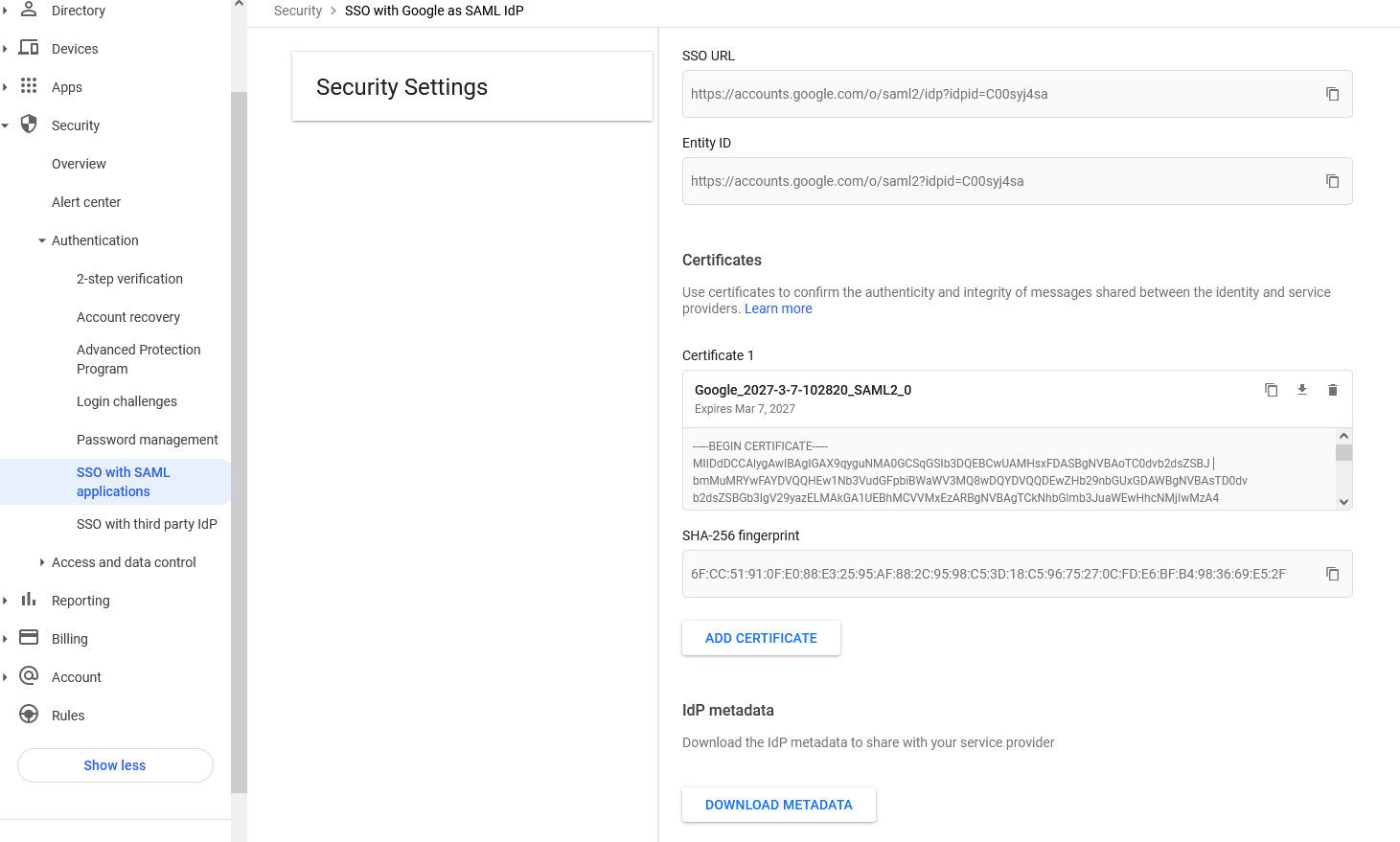
First, let’s get the SAML metadata that contains essential information to enable your AWS account to authenticate the IdP and locate the necessary communication endpoint locations. Complete the following steps:

  1. Log in to the Google Workspace Admin console.
  2. On the Admin console home page, under Security in the navigation pane, choose Authentication and SSO with SAML applications.
  3. Under IdP metadata, choose Download Metadata.

Create an IAM IdP with Google as SAML IdP

You now configure Azure AD as your SAML IdP via the IAM console. Complete the following steps:

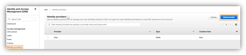
  1. On the IAM console, choose Identity providers in the navigation pane.
  2. Choose Add provider.
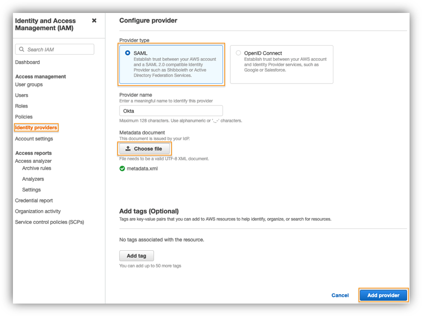
  3. For Configure provider, select SAML.
  4. For Provider name, enter a name for the IdP (such as Google).
  5. For Metadata document, choose Choose file and specify the SAML metadata document that you downloaded.
  6. Choose Add provider.
  7. Document the Amazon Resource Name (ARN) by viewing the IdP you just created.

The ARN should looks similar to arn:aws:iam::<YOURACCOUNTNUMBER>:saml-provider/Google. We need this ARN to configure claim rules later in this post.

Configure IAM policies for QuickSight roles

In this step, we create three IAM policies for different role permissions in QuickSight:

  • QuickSight-Federated-Admin
  • QuickSight-Federated-Author
  • QuickSight-Federated-Reader

Use the following steps to set up the QuickSight-Federated-Admin policy. This policy grants admin privileges in QuickSight to the federated user:

  1. On the IAM console, choose Policies.
  2. Choose Create policy.
  3. Choose JSON and replace the existing text with the following code:
    {
        “Version”: “2012-10-17”,
        “Statement”: [
            {
                “Effect”: “Allow”,
                “Action”: “quicksight:CreateAdmin”,
                “Resource”: “*”
            }
        ]
    }

  4. Choose Review policy.
  5. For Name, enter QuickSight-Federated-Admin.
  6. Choose Create policy.
  7. Repeat these steps to create QuickSight-Federated-Author, and use the following policy to grant author privileges in QuickSight to the federated user:
    {
        “Version”: “2012-10-17”,
        “Statement”: [
            {
                “Effect”: “Allow”,
                “Action”: “quicksight:CreateUser”,
                “Resource”: “*”
            }
        ]
    }

  8. Repeat the steps to create QuickSight-Federated-Reader, and use the following policy to grant reader privileges in QuickSight to the federated user:
    {
        “Version”: "2012-10-17",
        "Statement": [
            {
                "Effect": "Allow",
                "Action": "quicksight:CreateReader",
                "Resource": "*"
            }
        ]
    }

Configure IAM QuickSight roles for federated users

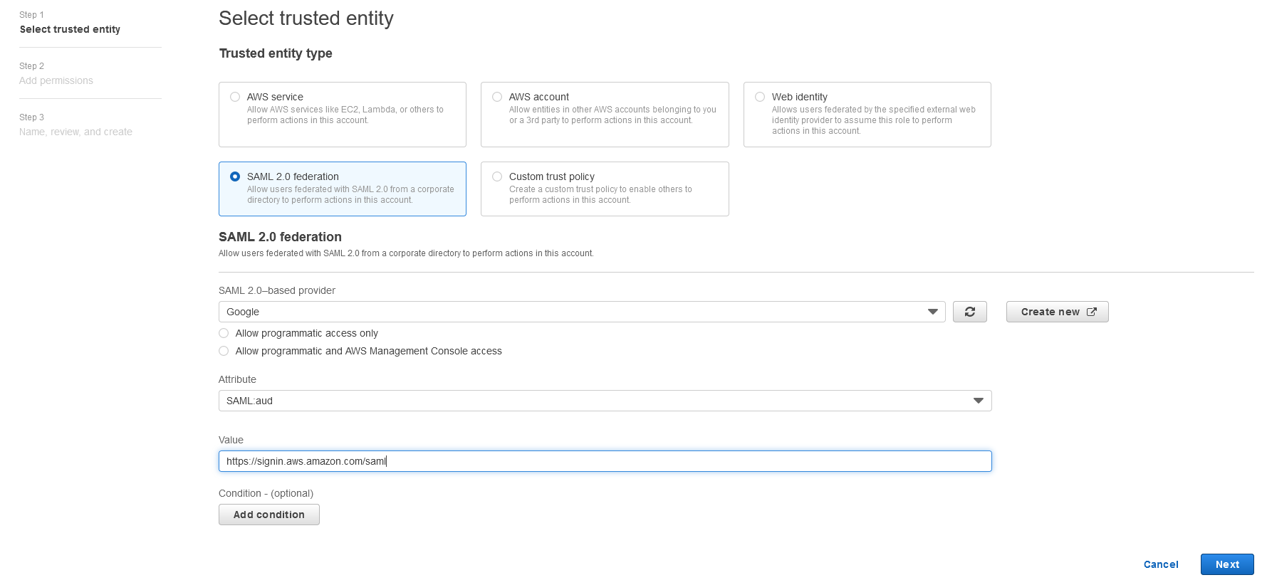
Next, create the roles that Google IdP users assume when federating into QuickSight. The following steps set up the admin role:

  1. On the IAM console, choose Roles in the navigation pane.
  2. Choose Create role.
  3. For Trusted entity type, choose SAML 2.0 federation.
  4. For SAML provider, choose the provider you created earlier (Google).
  5. For Attribute, choose SAML:aud.
  6. For Value, enter https://signin.aws.amazon.com/saml.
  7. Choose Next.
  8. On the Add permissions page, select the QuickSight-Federated-Admin IAM policy you created earlier.
  9. Choose Next.
  10. For Role name, enter QuickSight-Admin-Role.
  11. For Role description, enter a description.
  12. Choose Create role.
  13. On the IAM console, in the navigation pane, choose Roles.
  14. Choose the QuickSight-Admin-Role role you created to open the role’s properties.
  15. On the Trust relationships tab, choose Edit trust relationship.
  16. Under Trusted entities, verify that the IdP you created is listed.
  17. Under Condition, verify that SAML:aud with a value of https://signin.aws.amazon.com/saml is present.
  18. Repeat these steps to create author and reader roles and attach the appropriate policies:
    1. For QuickSight-Author-Role, use the policy QuickSight-Federated-Author.
    2. For QuickSight-Reader-Role, use the policy QuickSight-Federated-Reader.
  19. Navigate to the newly created roles and note the ARNs for them.

We use these ARNs to configure claims rules later in this post. They are in the following format:

  • arn:aws:iam:: <YOURACCOUNTNUMBER>:role/QuickSight-Admin-Role
  • arn:aws:iam:: <YOURACCOUNTNUMBER>:role/QuickSight-Author-Role
  • arn:aws:iam:: <YOURACCOUNTNUMBER>:role/QuickSight-Reader-Role

Create a custom user attribute in Google Workspace

Now let’s create a custom user attribute in your Google Workspace. This allows us to add the SAML attributes that the AWS Management Console expects in order to allow a SAML-based authentication.

  1. Log in to Google Admin console with admin credentials.
  2. Under Directory, choose Users.
  3. On the More options menu, choose Manage custom attributes.
  4. Choose Add Custom Attribute.
  5. For Select type of trusted entity, choose SAML 2.0 federation.
  6. Configure the custom attribute as follows:
    1. Category: Amazon
    2. Description: Amazon Custom Attributes
  7. For Custom fields, enter the following:
    1. Name: Role
    2. Info type: Text
    3. Visibility: Visible to user and admin
    4. No. of values: Multi-value
  8. Choose Add.

The new category appears on the Manage user attributes page.

Add the AWS SAML attributes to the Google Workspace user profile

Now that we have configured a custom user attribute, let’s add the SAML attributes that we noted earlier to the Google Workspace user profile.

  1. While logged in to the Google Admin console with admin credentials, navigate to the Users page.
  2. In the Users list, find the user. If you need help, see Find a user account.
  3. Choose the user’s name to open their account page.
  4. Choose User information.
  5. Choose custom attribute you recently created, named Amazon.
  6. Add a value to this custom attribute noted earlier in the following format: <AWS Role ARN>,<AWS provider/IdP ARN>.
  7. Choose Save.

Set up the AWS SAML app in Google Workspace

Now that we have everything in place, we’re ready to create a SAML app within our Google Workspace account and provide the QuickSight instance starting URL. This provides the entry point for Google Workspace users to SSO into the QuickSight instance.

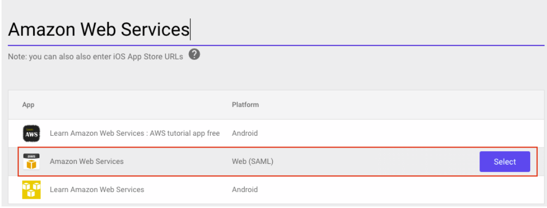
  1. While logged in to Google Admin console with admin credentials, under Apps, choose Web and mobile apps.
  2. Choose Add App, and Search for apps.
  3. Enter Amazon Web Services in the search field.
  4. In the search results, hover over the Amazon Web Services SAML app and choose Select.
  5. On the Google Identity Provider details page, choose Continue.
  6. On the Service provider details page, the ACS URL and Entity ID values for Amazon Web Services are configured by default.
  7. For Start URL, enter https://quicksight.aws.amazon.com.
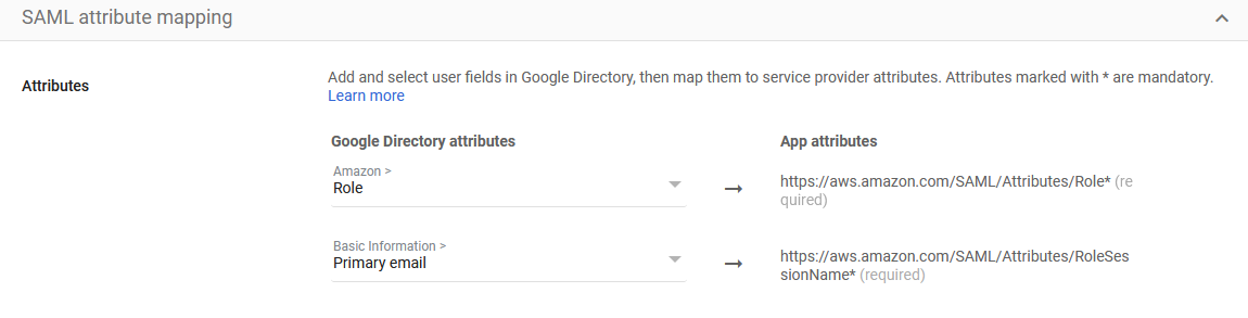
  8. On the Attribute Mapping page, choose the Select field menu and map the following Google directory attributes to their corresponding Amazon Web Services attributes:

    Google Directory Attribute Amazon Web Services Attribute
    Basic Information > Primary Email https://aws.amazon.com/SAML/Attributes/RoleSessionName
    Amazon > Role https://aws.amazon.com/SAML/Attributes/Role

  1. Choose Finish.

Grant access to users in Google Workspace

When the SAML app is created in Google workspace, it’s turned off by default. This means for users logged in to their Google Workspace account, the SAML app isn’t visible to them. We now enable the AWS SAML app to your Google Workspace users.

  1. While logged in to the Google Admin console with admin credentials, navigate to the Web and mobile apps page.
  2. Choose Amazon Web Services.

  3. Choose User access.
  4. To turn on a service for everyone in your organization, choose ON for everyone.
  5. Choose Save.

If you don’t want to activate this application for all users, you can alternatively grant access to a subset of users by using Google Workspace organizational units.

Verify federated access to the QuickSight instance

To test your SAML 2.0-based authentication with QuickSight for users in your existing IDP (Google Workspace), complete the following steps:

  1. Open a new browser session, for example, using Chrome, in a new incognito window.
  2. Log in to your Google Workspace account (for the purpose of this demo, we use the Google Workspace admin account).
  3. Choose Amazon Web Services from the list of Google apps.

Conclusion

This post provided a step-by-step guide for configuring Google Workspace as your IdP, and using IAM roles to enable SSO to QuickSight. Now your users have a seamless sign-in experience to QuickSight and have the appropriate level of access related to their role.

Although this post demonstrated the integration of IAM and Google Workspace, you can replicate this solution using your choice of SAML 2.0 IdPs. For other supported federation options, see Using identity federation and single sign-on (SSO) with Amazon QuickSight.

To get answers to your questions related to QuickSight, refer to the QuickSight Community.

If you have any questions or feedback, please leave a comment.


About the Authors

Sriharsh Adari is a Senior Solutions Architect at Amazon Web Services (AWS), where he helps customers work backwards from business outcomes to develop innovative solutions on AWS. Over the years, he has helped multiple customers on data platform transformations across industry verticals. His core area of expertise include Technology Strategy, Data Analytics, and Data Science. In his spare time, he enjoys playing sports, binge-watching TV shows, and playing Tabla.

Srikanth Baheti is a Specialized World Wide Sr. Solution Architect for Amazon QuickSight. He started his career as a consultant and worked for multiple private and government organizations. Later he worked for PerkinElmer Health and Sciences & eResearch Technology Inc, where he was responsible for designing and developing high traffic web applications, highly scalable and maintainable data pipelines for reporting platforms using AWS services and Serverless computing.

Tips and tricks for high-performant dashboards in Amazon QuickSight

Post Syndicated from Shekhar Kopuri original https://aws.amazon.com/blogs/big-data/tips-and-tricks-for-high-performant-dashboards-in-amazon-quicksight/

Amazon QuickSight is cloud-native business intelligence (BI) service. QuickSight automatically optimizes queries and execution to help dashboards load quickly, but you can make your dashboard loads even faster and make sure you’re getting the best possible performance by following the tips and tricks outlined in this post.

Data flow and execution of QuickSight dashboard loads

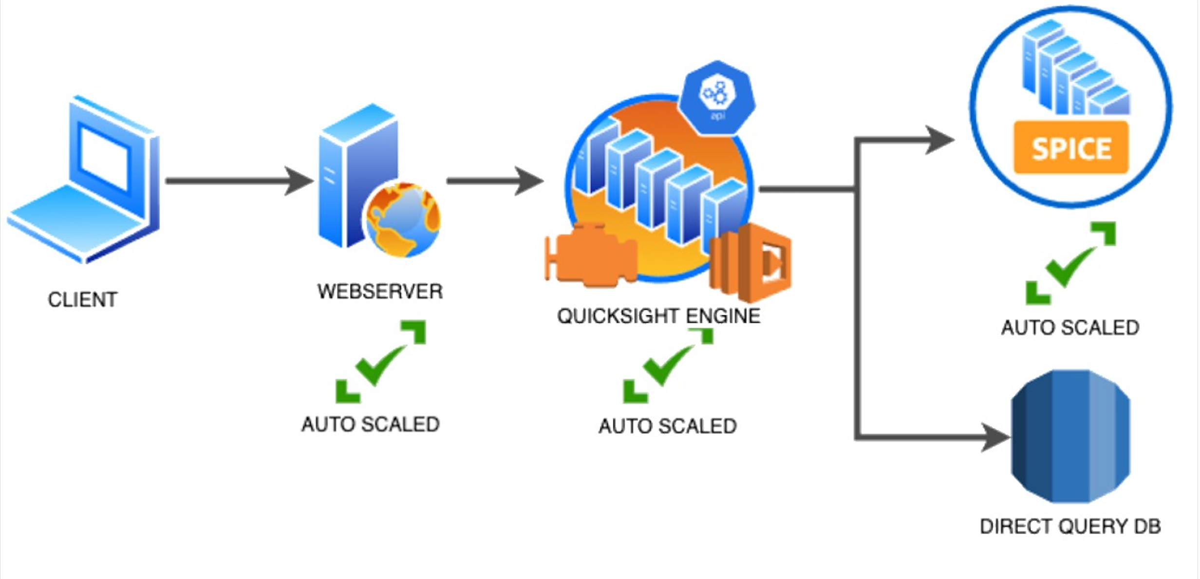
The data flow in QuickSight starts from the client browser to the web server and then flows to the QuickSight engine, which in some cases executes queries against SPICE—a Super-fast, Parallel, In-memory Calculation Engine—or in other cases directly against the database. SPICE uses a combination of columnar storage, in-memory technologies enabled through the latest hardware innovations, and machine code generation to run interactive queries on large datasets and get rapid responses.

The web server, QuickSight engine, and SPICE are auto scaled by QuickSight. This is a fully managed service—you don’t need to worry about provisioning or managing infrastructure when you want to scale up a particular dashboard from tens to thousands of users on SPICE. Dashboards built against direct query data sources may require provisioning or managing infrastructure on the customer side.

The following diagram illustrates the data flow:

Let’s look at the general execution process to understand the implications:

  • A request is triggered in the browser, leading to several static assets such as JavaScript, fonts, and images being downloaded.
  • All the metadata (such as visual configurations and layout) is fetched for the dashboard.
  • Queries are performed, which may include setting up row-level and column-level security, or fetching dynamic control values, default parameters, and all values of drop-downs in filter controls.
  • Up to your concurrency limit, the queries to render your visuals run in a specific sequence (described later in this post). If you’re using SPICE, the concurrency of queries is much higher. Pagination within visuals may lead to additional queries.
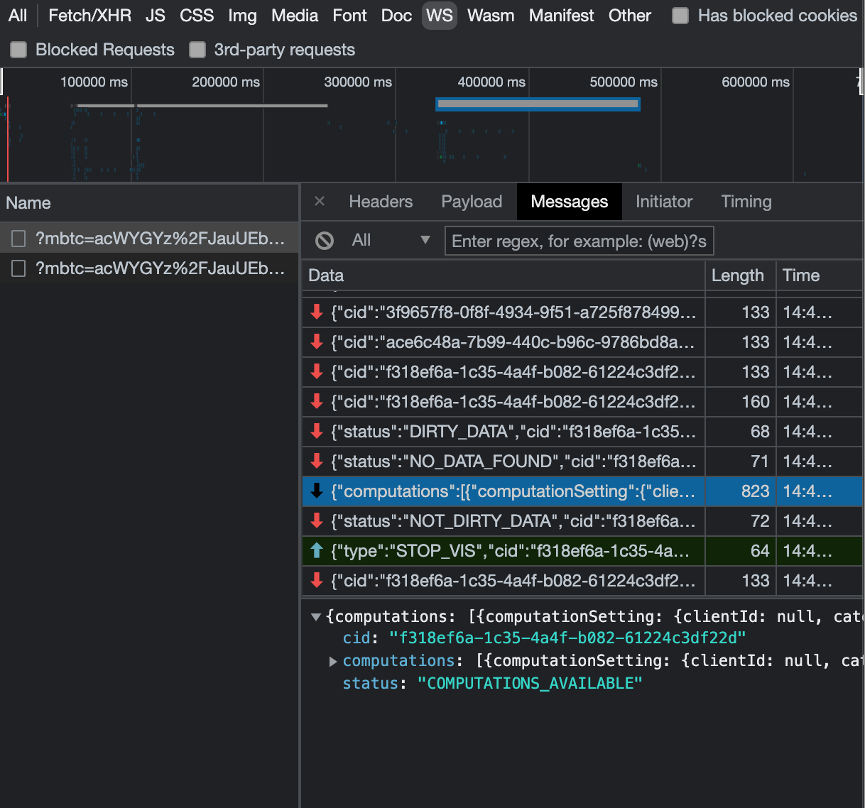
The actual execution is more complex and depends on how dashboards are configured and other factors such as the data source types, Direct Query vs. SPICE, cardinality of fields and how often data is getting refreshed etc.  Many operations run in parallel and all visual-related queries are run via WebSocket, as shown in the following screenshot. Many of the steps run in the end-user’s browser, therefore there are limitations such as the number of sequences and workloads that can be pushed onto the browser. Performance may also be slightly different based on the browser type because each browser handles contention differently.

Now let’s look at many great tips that can improve your dashboard’s performance!

SPICE

Utilizing the capabilities of SPICE when possible is a great way to boost overall performance because SPICE manages scaling as well as caching results for you. We recommend using SPICE whenever possible.

Metadata

As seen in the preceding execution sequence, QuickSight fetches metadata up front for a given dashboard during the initial load. We recommend the following actions regarding metadata.

Remove unused datasets from analysis

Datasets that may have been used in the past but have no visual associated with the dashboard anymore add to the metadata payload unnecessarily. It’s likely to impact to dashboard performance.

Make sure your row-level and column-level security is performant

Row-Level security, column-level security and dynamic default parameters each require lookups to take place before the visual queries are issued. When possible, try to limit the number and the complexity of your rules datasets to help these lookups execute faster. Use SPICE for your rules dataset when possible. If you must use a direct query, make sure that the queries are optimal and that the data source you’re querying is scaled appropriately up front.

For embedded dashboards, a great way to optimize row-level security lookups is by utilizing session tags for row-level security paired with an anonymous identity. Similarly, dynamic default parameters, if used, can be evaluated in the host application up front and passed using the embedding SDK.

Calculated functions

In this section, we offer tips regarding calculated functions.

Move calculations to the data prep stage

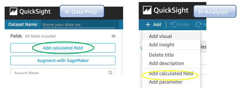
QuickSight allows you to add calculated fields in the data prep or analysis experiences. We strongly encourage you to move as many calculations as possible to the data prep stage which will allow QuickSight to materialize calculations which do not contain aggregation or parameters into the SPICE dataset. Materializing calculated fields in the dataset helps you reduce the runtime calculations, which improves query performance. Even if you are using aggregation or parameters in your calculation, it might still be possible to move parts of the calculations to data prep. For instance, if you have a formula like the following:

You can remove the sum() and just keep the ifelse(), which will allow QuickSight to materialize (precompute) it and save it as a real field in your SPICE dataset. Then you can either add another calculation which sums it up, or just use sum aggregation once you add it to your visuals.

Generally materializing calculations that use complex ifelse logic or do string manipulation/lookups will result in the greatest improvements in dashboard performance.

Implement the simplified ifelse syntax

The ifelse function supports simplified statements. For example, you might start with the following statement:

The following simplified statement is more performant:

Use the toString() function judiciously

The toString() function has a much lower performance and is much heavier on the database engine than a simple integer or number-based arithmatic calculations. Therefore, you should use it sparingly.

Know when nulls are returned by the system and use null value customization

Most authors make sure that null conditions on calculated fields are handled gracefully. QuickSight often handles nulls gracefully for you. You can use that to your advantage and make the calculations simpler. In the following example, the division by 0 is already handled by QuickSight:

You can write the preceding code as the following:

If you need to represent nulls on visuals with a static string, QuickSight allows you to set custom values when a null value is returned in a visual configuration. In the preceding example, you could just set a custom value of 0 in the formatting option. Removing such handling from the calculated fields can significantly help query performance.

On-sheet filters vs. parameters

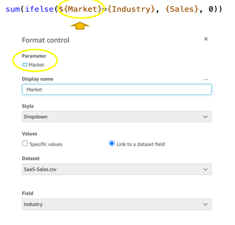
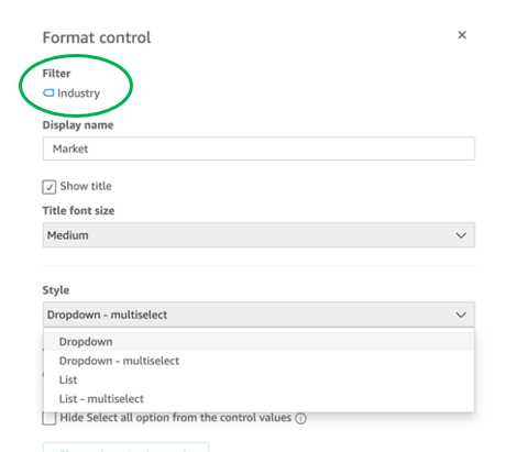
Parameters are seemingly a very simple construct but they can quickly get complicated, especially when used in nested calculation functions or when used in controls. Parameters are all evaluated on the fly, forcing all the dependencies to be handled real time. Ask yourself if each parameter is really required. In some cases, you may be able to replace them with simple dropdown control, as shown in the following example for $market.

Instead of creating a control parameter to use in a calculated field, you might be able to use the field with a dropdown filter control.

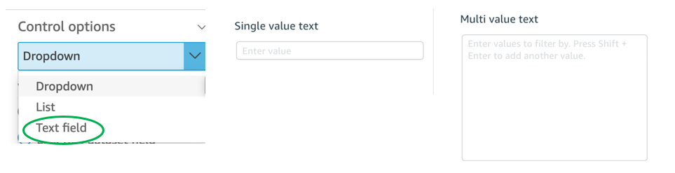
Text field vs. Dropdown (or List) filter controls

When you are designing an analysis, you can add a filter control for the visuals you want to filter. if the data type of the field is string, you have several choices for the type of control filter. Text field which displays a text box where you can enter a single entry or multiple entries is suggested for the better performance, rather than Dropdown (or List) which requires to fetch the values to populate a list that you can select a single or multiple values.

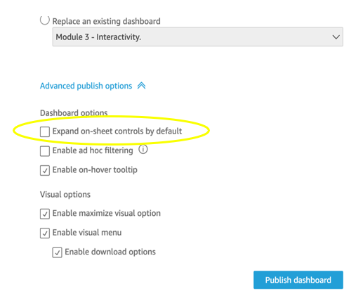
On-sheet controls

The control panel at the top of the dashboard is collapsible by default, but this setting allows you to have an expanded state while publishing the dashboard. If this setting is enabled, QuickSight prioritizes the calls in order to fetch the controls’ values before the visual loads. If any of the controls have high cardinality, it could impact the performance of loading the dashboard. Evaluate this need against the fact that QuickSight persists last-used control values and the reader might not actually need to adjust controls as a first step.

Visual types: Charts

In this section, we provide advice when using Charts.

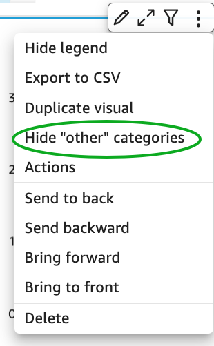
Use ‘Hide the “other” category’ when your dimension has less than the cutoff limit

You can choose to limit how many data points you want to display in your visual, before they are added to the other category. This category contains the aggregated data for all the data beyond the cutoff limit for the visual type you are using – either the one you impose or the one based on display limits. If you know your dimension has less than the cutoff limit, use this option. This will improve your dashboard performance.

The other category does not show on scatter plots, heat maps, maps, tables (tabular reports), or key performance indicators (KPIs). It also doesn’t show on line charts when the x-axis is a date.

Visual types: Tables and pivot tables

In this section, we provide advice when using tables and pivot tables.

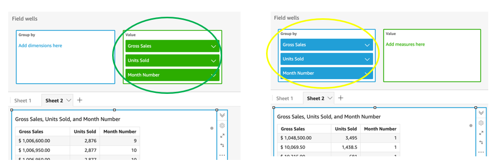
Use the Values field well when displaying a raw table view

If you want to output all the raw data into table, you can use Group by fields, Values fields, or a mix of them. The most performant approach is set every field into Values. When using Group by, a query is first run under the hood followed by the Group by function, therefore all the data is pulled from the database, which is expensive.

Deploy a minimal set of rows, columns, metrics, and table calculations

If you include too many combinations of rows, columns, metrics, and table calculations in one pivot table, you risk overwhelming the viewer. You can also run into the computational limitations of the underlying database. To reduce the level of complexity and potential errors, you can take the following actions:

  • Apply filters to reduce the data included in for the visual
  • Use fewer fields in the Row and Column field wells
  • Use as few fields as possible in the Values field well
  • Create additional pivot tables so that each displays fewer metrics
  • Reduce subtotals, totals and conditional formatting when possible

Uncollapsed columns are always the simplest case and will likely remain more performant outside of a few cases.

Visual queries sequence

The execution of the individual visual sequence is left to right, then top to bottom. Understanding the sequence of execution can be helpful: you can rearrange visuals on your dashboard without losing the context. Place heavier visuals further down in the dashboard, and place lightweight KPI and insight visuals near the top to display “above-the-fold” content sooner, which improves the dashboard performance’s perception for your readers.

Embedding

Our final set of recommendations are in regards to embedding.

Remove user management flows from the critical path

Most times, user management and authentication flows (such as DescribeUser and RegisterUser APIs) can run asynchronously on the host application.

Consider registering the user in advance before the actual embedding, so that the overhead is removed from every analytics page visit.

Authenticate the user on your website in advance, and acquire any Amazon Cognito or AWS Security Token Service (Amazon STS) session tokens (if required) in advance (for example, at user login time or home page visit). This reduces additional runtime latency overhead when a user visits an analytics page.

Move workloads from clients to the web server or backend services

If a QuickSight dashboard is embedded on a webpage on the host application, which performs other activities too, play close attention to the sequence of API calls on the host. The QuickSight dashboard load might be gated by other heavy API calls on the host application. Move the logic to the web server or backend services as much as possible to limit contention on the browser.

Don’t tear down the embedding iFrame when the user navigates away from analytics section

When the user moves temporarily to a non-analytics page of your web application (especially in single-page applications), instead of removing the embedding iframe from DOM, you can hide it from the user while keeping the iFrame in the page DOM elements. This allows you to resume the same session when the user navigates back to analytics section of your application, and they don’t need to wait for reload.

Use navigateToDashboard() and navigateToSheet() whenever possible

If you have multiple dashboards on your host application that don’t need to load concurrently, you can optimize the authentication flow by utilizing two APIs we expose, navigateToDashboard() or navigateToSheet(), in our JavaScript SDK. These APIs reuse the same iFrame for each load, while reusing the authentication token.

This technique has proven to be very effective for many of our embedding users.

For more information about these APIs, refer to Amazon QuickSight Embedding SDK.

Conclusion

In this post, we shared some tips and tricks for tuning the performance of your QuickSight dashboards. In 2021, we doubled our SPICE data limits to 500 million rows of data per dataset. In addition, incremental data refresh is available for SQL-based data sources such as Amazon Redshift, Amazon Athena, Amazon RDS, Amazon Aurora, PostgreSQL, MySQL, Oracle, SQL Server, MariaDB, Presto, Teradata or Snowflake up to every 15 minutes, which cuts down time between data updates by 75%. In 2022, we continue to innovate on your behalf to make QuickSight dashboard loads even more performant.

We look forward to your feedback on how these tips and tricks helped your dashboards load faster.


About the Authors

Shekhar Kopuri is a Senior Software Development Manager for Amazon QuickSight. He leads the front platform engineering team that focusses on various aspects of front end experience including website performance. Before joining AWS, Shekhar led development of multiple provisioning and activation network OSS applications for a large global telecommunications service provider.

Blake Carroll is a Senior Frontend Engineer for Amazon QuickSight. He works with the frontend platform engineering team with a focus on website performance and has previously been the frontend lead for initial reporting and theming functionality in QuickSight. Prior to joining Amazon, Blake was a co-founder in the digital interactive agency space working with national brands to produce creative web experiences.

Vijay Chaudhari is a Senior Software Development Engineer for Amazon QuickSight, AWS’ cloud-native, fully managed BI service. Vijay started his career with IBM, writing software for the Information Management group. At Amazon, he has built backend applications for retail systems, and near real-time data pre-computation, reporting and analytics systems at Amazon scale. He is passionate about learning and solving new customer problems, and helping them adopt cloud native technologies.

Wakana Vilquin-Sakashita is Specialist Solution Architect for Amazon QuickSight. She works closely with customers to help making sense of the data through visualization. Previously Wakana worked for S&P Global  assisting customers to access data, insights and researches relevant for their business.

Analyze Amazon Ion datasets using Amazon Athena

Post Syndicated from Pathik Shah original https://aws.amazon.com/blogs/big-data/analyze-amazon-ion-datasets-using-amazon-athena/

Amazon Athena is an interactive query service that makes it easy to analyze data in Amazon Simple Storage Service (Amazon S3) using standard SQL. Athena is serverless, so there is no infrastructure to manage, and you pay only for the queries that you run.

Amazon Ion is a richly typed, self-describing, hierarchical data serialization format offering interchangeable binary and text representations. The text format extends JSON (meaning all JSON files are valid Ion files), and is easy to read and author, supporting rapid prototyping. The binary representation is efficient to store, transmit, and skip-scan parse. The rich type system provides unambiguous semantics for long-term preservation of data that can survive multiple generations of software evolution.

Athena now supports querying and writing data in Ion format. The Ion format is currently used by internal Amazon teams, by external services such as Amazon Quantum Ledger Database (Amazon QLDB) and Amazon DynamoDB (which can be exported into Ion), and in the open-source SQL query language PartiQL.

In this post, we discuss use cases and the unique features Ion offers, followed by examples of querying Ion with Athena. For demonstration purposes, we use the transformed version of the City Lots San Francisco dataset.

Features of Ion

In this section, we discuss some of the unique features that Ion offers:

  • Type system
  • Dual format
  • Efficiency gains
  • Skip scanning

Type system

Ion extends JSON, adding support for more precise data types to improve interpretability, simplify processing, and avoid rounding errors. These high precision numeric types are essential for financial services, where fractions of a cent on every transaction add up. Data types that are added are arbitrary-size integers, binary floating-point numbers, infinite-precision decimals, timestamps, CLOBS, and BLOBS.

Dual format

Users can be presented with a familiar text-based representation while benefiting from the performance efficiencies of a binary format. The interoperability between the two formats enables you to rapidly discover, digest, and interpret data in a familiar JSON-like representation, while underlying applications benefit from a reduction in storage, memory, network bandwidth, and latency from the binary format. This means you can write plain text queries that run against both text-based and binary-based Ion. You can rewrite parts of your data in text-based Ion when you need human readable data during development and switch to binary in production.

When debugging a process, the ability for systems engineers to locate data and understand it as quickly as possible is vital. Ion provides mechanisms to move between binary and a text-based representation, optimizing for both the human and the machine. Athena supports querying and writing data in both of these Ion formats. The following is an example Ion text document taken from the transformed version of the citylots dataset:

{ "type": "Feature"
, "properties": { "MAPBLKLOT": "0004002"
                 ,"BLKLOT": "0004002"
                 ,"BLOCK_NUM": "0004"
                 , "LOT_NUM": "002"
                 , "FROM_ST": "0"
                 , "TO_ST": "0"
                 , "STREET": "UNKNOWN"
                 , "ST_TYPE": null
                 , "ODD_EVEN": "E" }
, "geometry": { "type": "Polygon"
               , "coordinates": [ [ [ -122.415701204606876, 37.808327252671461, 0.0 ],
                                    [ -122.415760743593196, 37.808630700240904, 0.0 ],
                                    [ -122.413787891332404, 37.808566801319841, 0.0 ],
                                    [ -122.415701204606876, 37.808327252671461, 0.0 ] ] ] } }

Efficiency gains

Binary-encoded Ion reduces file size by moving repeated values, such as field names, into a symbol table. Symbol tables reduce CPU and read latency by limiting the validation of character encoding to the single instance of the value in the symbol table.

For example, a company that operates at Amazon’s scale can produce large volumes of application logs. When compressing Ion and JSON logs, we noticed approximately 35% less CPU time to compress the log, which produced an average of roughly 26% smaller files. Log files are critical when needed but costly to retain, so the reduction in file sizes combined with the read performance gains from symbol tables helps when handling these logs. The following is an example of file size reduction with the citylots JSON dataset when converted to Ion binary with GZIP and ZSTD compression:
77MB    citylots.ion
 17MB    citylots.ion.gz
 15MB    citylots.ion.zst
181MB    citylots.json
 22MB    citylots.json.gz
 18MB    citylots.json.zst

Skip-scanning

In a textual format, every byte must be read and interpreted, but because Ion’s binary format is a TLV (type-length-value) encoding, an application may skip over elements that aren’t needed. This reduces query and application processing costs correlated with the proportion of unexamined fields.
For example, forensic analysis of application log data involves reading large volumes of data where only a fraction of the data is needed for diagnosis. In these scenarios, skip-scanning allows the binary Ion reader to move past irrelevant fields without the cost of reading the element stored within a field. This results in users experiencing lower resource usage and quicker response times.

Query Ion datasets using Athena

Athena now supports querying and creating Ion-formatted datasets via an Ion-specific SerDe, which in conjunction with IonInputFormat and IonOutputFormat allows you to read and write valid Ion data. Deserialization allows you to run SELECT queries on the Ion data so that it can be queried to gain insights. Serialization through CTAS or INSERT INTO queries allows you to copy datasets from existing tables’ values or generate new data in the Ion format.

The interchangeable nature of Ion text and Ion binary means that Athena can read datasets that contain both types of files. Because Ion is a superset of JSON, a table using the Ion SerDe can also include JSON files. Unlike the JSON SerDe, where every new line character indicates a new row, the Ion SerDe uses a combination of closing brackets and new line characters to determine new rows. This means that if each JSON record in your source documents isn’t on a single line, these files can now be read in Athena via the Ion SerDe.

Create external tables

Athena supports querying Ion-based datasets by defining AWS Glue tables with the user-defined metadata. Let’s start with an example of creating an external table for a dataset stored in Ion text. The following is a sample row from the citylots dataset:

{
    type:"Feature",
    properties:{
        mapblklot:"0579021",
        blklot:"0579024",
        block_num:"0579",
        lot_num:"024",
        from_st:"2160",
        to_st:"2160",
        street:"PACIFIC",
        st_type:"AVE",
        odd_even:"E"
    },
    geometry:{
        type:"Polygon",coordinates:[[[-122.4308798855922, ...]]]
    }
}

To create an external table that has its data stored in Ion, you have two syntactic options.

First, you can specify STORED AS ION. This is a more concise method, and is best used for simple cases, when no additional properties are required. See the following code:

CREATE EXTERNAL TABLE city_lots_ion1 (
  type STRING, 
  properties struct<
    mapblklot:string,
    blklot:string,
    block_num:string,
    lot_num:string,
    from_st:string,
    to_st:string,
    street:string,
    st_type:string,
    odd_even:string>, 
  geometry struct<
    type:string,
    coordinates:array<array<array<decimal(18,15)>>>,
    multi_coordinates:array<array<array<array<decimal(18,15)>>>>>
)
STORED AS ION
LOCATION 's3://aws-bigdata-blog/artifacts/athena-ion-blog/city_lots_ion_binary/'

Alternatively, you can explicitly specify the Ion classpaths in ROW FORMAT SERDE, INPUTFORMAT, and OUTPUTFORMAT. Unlike the first method, you can specify a SERDEPROPERTIES clause here. In our example DDL, we added a SerDe property that allows values that are outside of the Hive data type ranges to overflow rather than fail the query:

CREATE EXTERNAL TABLE city_lots_ion2(
  type STRING, 
  properties struct<
    mapblklot:string,
    blklot:string,
    block_num:string,
    lot_num:string,
    from_st:string,
    to_st:string,
    street:string,
    st_type:string,
    odd_even:string>, 
  geometry struct<
    type:string,
    coordinates:array<array<array<decimal(18,15)>>>,
    multi_coordinates:array<array<array<array<decimal(18,15)>>>>>
)
ROW FORMAT SERDE 
  'com.amazon.ionhiveserde.IonHiveSerDe'
WITH SERDEPROPERTIES (
 'ion.fail_on_overflow'='false'
 )
STORED AS INPUTFORMAT 
  'com.amazon.ionhiveserde.formats.IonInputFormat' 
OUTPUTFORMAT 
  'com.amazon.ionhiveserde.formats.IonOutputFormat'
LOCATION
  's3://aws-bigdata-blog/artifacts/athena-ion-blog/city_lots_ion_binary/'

Athena converts STORED AS ION into the explicit classpaths, so both tables look similar in the metastore. If we look in AWS Glue, we see both tables we just created have the same input format, output format, and SerDe serialization library.

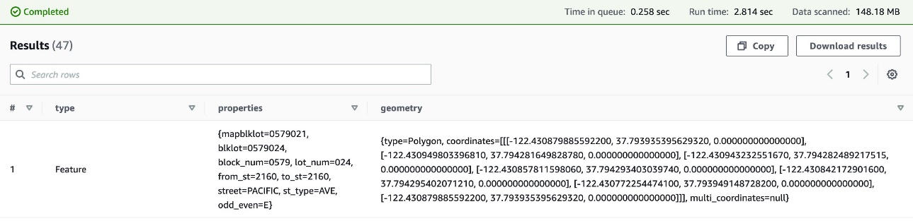
Now that our table is created, we can run standard SELECT queries on the city_lots_ion table. Let’s run a query that specifies the block_num from our example row of Ion data to verify that we can read from the table:

-- QUERY
SELECT * FROM city_lots_ion1 WHERE properties.block_num='0579';

The following screenshot shows our results.

Use path extraction to read from specific fields

Athena supports further customization of how data is interpreted via SerDe properties. To specify these, you can add a WITH SERDEPROPERTIES clause, which is a subfield of the ROW FORMAT SERDE field.

In some situations, we may only care about some parts of the information. Let’s suppose we don’t want any of the geometry info from the citylots dataset, and only need a few of the fields in properties. One solution is to specify a search path using the path extractor SerDe property:

-- Path Extractor property
ion.<column>.path_extractor = <search path>

Path extractors are search paths that Athena uses to map the table columns to locations in the individual document. Full information on what can be done with path extractors is available on GitHub, but for our example, we focus on creating simple paths that use the names of each field as an index. In this case, the search path takes the form of a space-delimited set of indexes (and wraps it with parentheses) that indicate the location of each desired piece of information. We map the search paths to table columns by using the path extractor property.

By default, Athena builds path extractors dynamically based on column names unless overridden. This means that when we run our SELECT query on our city_lots_ion1 table, Athena builds the following search paths:

Default Extractors generated by Athena for city_lots_ion1.
-- Extracts the 'type' field to the 'type' column
    'ion.type.path_extractor' = '(type)'

-- Extracts the 'properties' field to the 'properties' column
    'ion.properties.path_extractor' = '(properties)'

-- Extracts the 'geometry' field to the 'geometry' column
    'ion.geometry.path_extractor' = '(geometry)'

Assuming we only care about the block and lot information from the properties struct, and the geometry type from the geometry struct, we can build search paths that map the desired fields from the row of data to table columns. First let’s build the search paths:

(properties mapblklot) - Search path for the mapblklot field in the properties struct
(properties blklot) - Search path for the blklot field in the properties struct
(properties block_num) - Search path for the block_num field in the properties struct
(properties lot_num) - Search path for the lot_num field in the properties struct
(geometry type) - Search path for the type field in the geometry struct

Now let’s map these search paths to table columns using the path extractor SerDe property. Because the search paths specify where to look for data, we are able to flatten and rename our datasets to better serve our purpose. For this example, let’s rename the mapblklot field to map_block_lot, blklot to block_lot, and the geometry type to shape:

 'ion.map_block_lot.path_extractor' = '(properties mapblklot)'
 'ion.block_lot.path_extractor' = '(properties blklot)'
 'ion.block_num.path_extractor' = '(properties block_num)'
 'ion.lot_num.path_extractor' = '(properties lot_num)'
 'ion.shape.path_extractor' = '(geometry type)'

Let’s put all of this together and create the city_blocks table:

CREATE EXTERNAL TABLE city_blocks (
    map_block_lot STRING,
    block_lot STRING,
    block_num STRING,
    lot_num STRING,
    shape STRING
)
ROW FORMAT SERDE
 'com.amazon.ionhiveserde.IonHiveSerDe'
WITH SERDEPROPERTIES (
 'ion.map_block_lot.path_extractor' = '(properties mapblklot)',
 'ion.block_lot.path_extractor' = '(properties blklot)', 
 'ion.block_num.path_extractor' = '(properties block_num)',
 'ion.lot_num.path_extractor' = '(properties lot_num)',
 'ion.shape.path_extractor' = '(geometry type)'
 )
STORED AS ION
LOCATION 's3://aws-bigdata-blog/artifacts/athena-ion-blog/city_lots_ion_binary/'

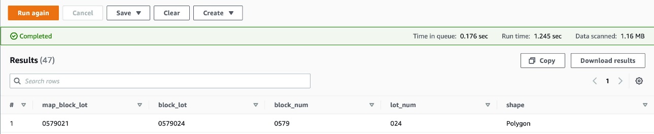
Now we can run a select query on the city_blocks table, and see the results:

-- Select Query
SELECT * FROM city_blocks WHERE block_num='0579';

Utilizing search paths in this way enables skip-scan parsing when reading from Ion binary files, which allows Athena to skip over the unneeded fields and reduces the overall time it takes to run the query.

Use CTAS and UNLOAD for data transformation

Athena supports CREATE TABLE AS SELECT (CTAS), which creates a new table in Athena from the results of a SELECT statement from another query. Athena also supports UNLOAD, which writes query results to Amazon S3 from a SELECT statement to the specified data format.

Both CTAS and UNLOAD have a property to specify a format and a compression type. This allows you to easily convert Ion datasets to other data formats, such as Parquet or ORC, and vice versa, without needing to set up a complex extract, transform, and load (ETL) job. This is beneficial for situations when you want to transform your data, or know you will run repeated queries on a subset of your data and want to use some of the benefits inherent to columnar formats. Combining it with path extractors is especially helpful, because we’re only storing the data that we need in the new format.

Let’s use CTAS to convert our city_blocks table from Ion to Parquet, and compress it via GZIP. Because we have path extractors set up for the city_blocks table, we only need to convert a small portion of the original dataset:

CREATE TABLE city_blocks_parquet_gzip
WITH (format = 'PARQUET', write_compression='GZIP')
AS SELECT * FROM city_blocks;

We can now run queries against the city_block_parquet_gzip table, and should see the same result. To test this out, let’s run the same SELECT query we ran before on the Parquet table:

SELECT * FROM city_blocks_parquet_gzip WHERE block_num='0579';

When converting tables from another format to Ion, Athena supports the following compression codecs: ZSTD, BZIP2, GZIP, SNAPPY, and NONE. In addition to adding Ion as a new format for CTAS, we added the ion_encoding property, which allows you to choose whether the output files are created in Ion text or Ion binary. This allows for serialization of data from other formats back into Ion.

Let’s convert the original city_lots JSON file back to Ion, but this time we specify that we want to use ZSTD compression and a binary encoding.

The JSON file can be found at following location: s3://aws-bigdata-blog/artifacts/athena-ion-blog/city_lots_json/

Because Ion is a superset of JSON, we can use the Ion SerDe to read this file:

CREATE EXTERNAL TABLE city_blocks_json_ion_serde (
    map_block_lot STRING,
    block_lot STRING,
    block_num STRING,
    lot_num STRING,
    shape STRING
)
ROW FORMAT SERDE
'com.amazon.ionhiveserde.IonHiveSerDe'
WITH SERDEPROPERTIES (
'ion.map_block_lot.path_extractor' = '(properties mapblklot)',
'ion.block_lot.path_extractor' = '(properties blklot)',
'ion.block_num.path_extractor' = '(properties block_num)',
'ion.lot_num.path_extractor' = '(properties lot_num)',
'ion.shape.path_extractor' = '(geometry type)'
)
STORED AS ION
LOCATION 's3://aws-bigdata-blog/artifacts/athena-ion-blog/city_lots_json/'

Now let’s copy this table into our desired Ion binary form:

CREATE TABLE city_blocks_ion_zstd
WITH (format = 'ION', write_compression='ZSTD', ion_encoding='BINARY')
AS SELECT * FROM city_blocks_parquet_gzip

Finally, let’s run our verification SELECT statement to verify everything was created properly:

SELECT * FROM city_blocks_ion_zstd WHERE block_num='0579'; 

Use UNLOAD to store Ion data in Amazon S3

Sometimes we just want to reformat the data and don’t need to store the additional metadata to query the table. In this case, we can use UNLOAD, which stores the results of the query in the specified format in an S3 bucket.

Let’s test it out, using UNLOAD to convert the drivers_names table from Ion to ORC, compress it via ZLIB, and store it to an S3 bucket:

UNLOAD (SELECT * FROM city_blocks_ion_zstd WHERE block_num='0579') 
TO 's3://<your-s3-bucket>/athena-ion-blog/unload/orc_zlib/'
WITH (format = 'ORC', compression='ZLIB')

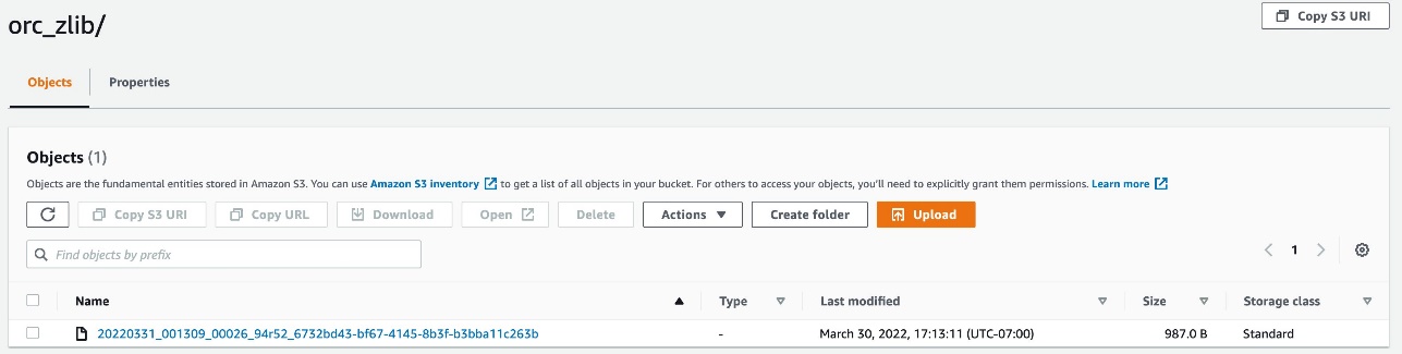
When you check in Amazon S3, you can find a new file in the ORC format.

Conclusion

This post talked about the new feature in Athena that allows you to query and create Ion datasets using standard SQL. We discussed use cases and unique features of the Ion format like type system, dual formats (Ion text and Ion binary), efficiency gains, and skip-scanning. You can get started with querying an Ion dataset stored in Amazon S3 by simply creating a table in Athena, and also converting existing datasets to Ion format and vice versa using CTAS and UNLOAD statements.

To learn more about querying Ion using Athena, refer to Amazon Ion Hive SerDe.

References


About the Authors

Pathik Shah is a Sr. Big Data Architect on Amazon Athena. He joined AWS in 2015 and has been focusing in the big data analytics space since then, helping customers build scalable and robust solutions using AWS analytics services.

Jacob Stein works on the Amazon Athena team as a Software Development Engineer. He led the project to add support for Ion in Athena. He loves working on technical problems unique to internet scale data, and is passionate about developing scalable solutions for distributed systems.

Giovanni Matteo Fumarola is the Engineering Manager of the Athena Data Lake and Storage team. He is an Apache Hadoop Committer and PMC member. He has been focusing in the big data analytics space since 2013.

Pete Ford is a Sr. Technical Program Manager at Amazon.

Use Amazon Redshift RA3 with managed storage in your modern data architecture

Post Syndicated from Bhanu Pittampally original https://aws.amazon.com/blogs/big-data/use-amazon-redshift-ra3-with-managed-storage-in-your-modern-data-architecture/

Amazon Redshift is a fully managed, petabyte-scale data warehouse service in the cloud. You can start with just a few hundred gigabytes of data and scale to a petabyte or more. This enables you to use your data to acquire new insights for your business and customers.

Over the years, Amazon Redshift has evolved a lot to meet our customer demands. Its journey started as a standalone data warehousing appliance that provided a low-cost, high-performance, cloud-based data warehouse. Support for Amazon Redshift Spectrum compute nodes was later added to extend your data warehouse to data lakes, and the concurrency scaling feature was added to support burst activity and scale your data warehouse to support thousands of queries concurrently. In its latest offering, Amazon Redshift runs on third-generation architecture where storage and compute layers are decoupled and scaled independent of each other. This latest generation powers the several modern data architecture patterns our customers are actively embracing to build flexible and scalable analytics platforms.

When spinning up a new instance of Amazon Redshift, you get to choose either Amazon Redshift Serverless, for when you need a data warehouse that can scale seamlessly and automatically as your demand evolves unpredictably, or you can choose an Amazon Redshift provisioned cluster for steady-state workloads and greater control over your Amazon Redshift cluster’s configuration.

An Amazon Redshift provisioned cluster is a collection of computing resources called nodes, which are organized into a group called a cluster. Each cluster runs the Amazon Redshift engine and contains one or more databases. Creating an Amazon Redshift cluster is the first step in your process of building an Amazon Redshift data warehouse. While launching a provisioned cluster, one option that you specify is the node type. The node type determines the CPU, RAM, storage capacity, and storage drive type for each node.

In this post, we cover the current generation node RA3 architecture, different RA3 node types, important capabilities that are available only on RA3 node types, and how you can upgrade your current Amazon Redshift node types to RA3.

Amazon Redshift RA3 nodes

RA3 nodes with managed storage enable you to optimize your data warehouse by scaling and paying for compute and managed storage independently. RA3 node types are the latest node type for Amazon Redshift. With RA3, you choose the number of nodes based on your performance requirements and only pay for the managed storage that you use. RA3 architecture gives you the ability to size your cluster based on the amount of data you process daily or the amount of data that you want to store in your warehouse; there is no need to account for both storage and processing needs together.

Other node types that we previously offered include the following:

  • Dense compute – DC2 nodes enable you to have compute-intensive data warehouses with local SSD storage included. You choose the number of nodes you need based on data size and performance requirements.
  • Dense storage (deprecated) – DS2 nodes enable you to create large data warehouses using hard disk drives (HDDs). If you’re using the DS2 node type, we strongly recommend that you upgrade to RA3 to get twice as much storage and improved performance for the same on-demand cost.

When you use the RA3 node size and choose your number of nodes, you can provision the compute independent of storage. RA3 nodes are built on the AWS Nitro System and feature high bandwidth networking and large high-performance SSDs as local caches. RA3 nodes use your workload patterns and advanced data management techniques to deliver the performance of local SSD while scaling storage automatically to Amazon Simple Storage Service (Amazon S3).

RA3 node types come in three different sizes to accommodate your analytical workloads. You can quickly start experimenting with the RA3 node type by creating a single-node ra3.xlplus cluster and explore various features that are available. If you’re running a medium-sized data warehouse, you can size your cluster with ra3.4xlarge nodes. For large data warehouses, you can start with ra3.16xlarge. The following table gives more information about RA3 node types and their specifications as of this writing.

Node Type vCPU

RAM

(GiB)

Default Slices Per Node Managed Storage Quota Per Node Node Range with Create Cluster Total Managed Storage Capacity
ra3.xlplus 4 32 2 32 TB 1-16 1024 TB
ra3.4xlarge 12 96 4 128 TB 2-32 8192 TB
ra3.16xlarge 48 384 16 128 TB 2-128 16384 TB

Amazon Redshift with managed storage

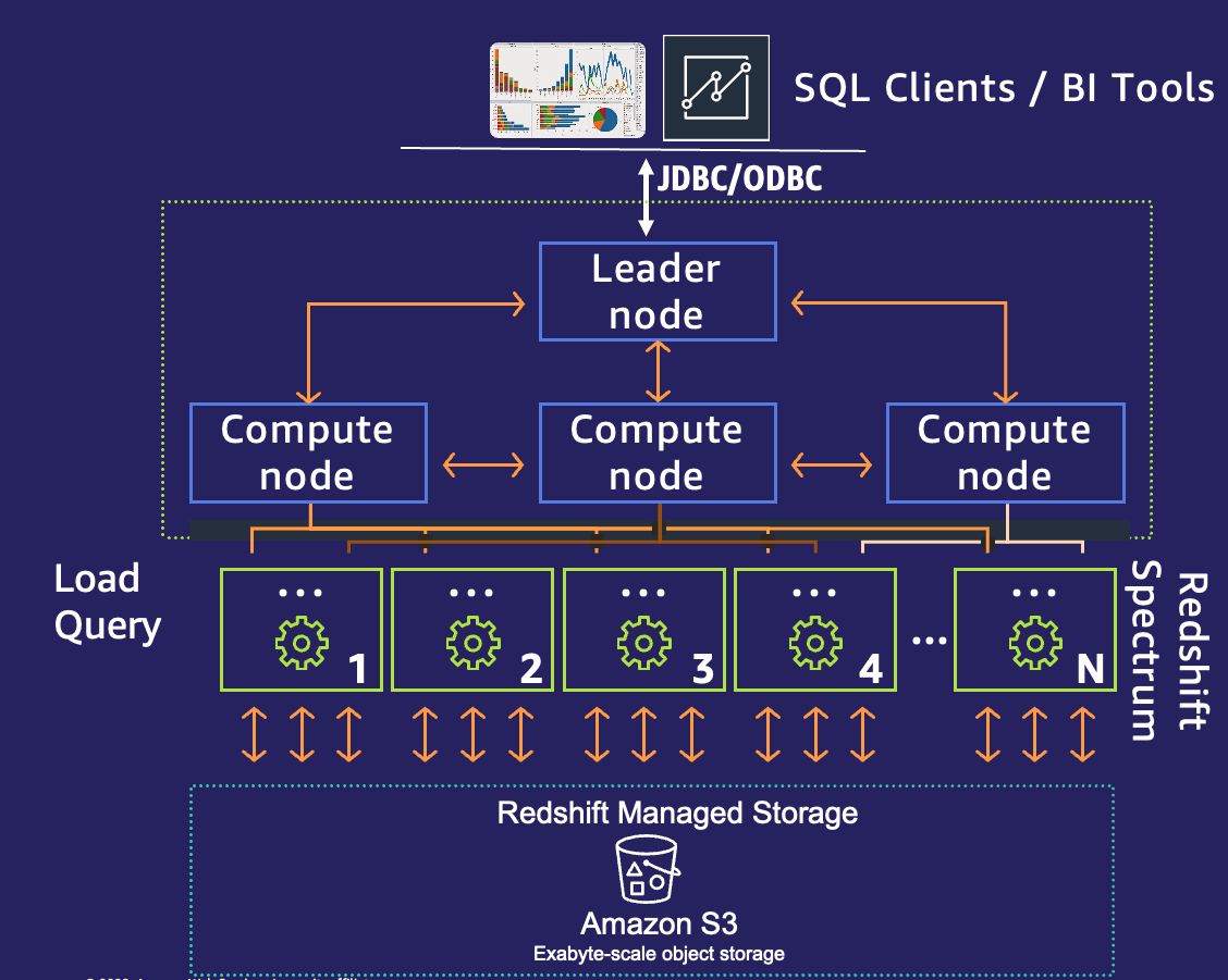
Amazon Redshift with a managed storage architecture (RMS) still boasts the same resiliency and industry-leading hardware. With managed storage, Amazon Redshift uses intelligent data prefetching and data evictions based on the temperature of your data. This method helps you decide where to store your most-queried data. Most frequently used blocks (hot data) are cached locally on SSD, and infrequently used blocks (cold data) are stored on an RMS layer backed by Amazon S3. The following diagram depicts the leader node, compute node, and Amazon Redshift managed storage.

In the following sections, we discuss the capabilities that Amazon Redshift RA3 with managed storage can provide.

Independently scale compute and storage

As the scale of an organization grows, data continues to grow—reaching petabytes. The amount of data you ingest into your Amazon Redshift data warehouse also grows. You may be looking for ways to cost-effectively analyze all your data and at the same time have control over choosing the right compute or storage resource at the right time. For customers who are looking to be cost conscientious and cost-effective, the RA3 platform provides the option to scale and pay for your compute and storage resources separately.

With RA3 instances with managed storage, you can choose the number of nodes based on your performance requirements, and only pay for the managed storage that you use. This gives you the flexibility to size your RA3 cluster based on the amount of data you process daily without increasing your storage costs. It allows you to pay per hour for the compute and separately scale your data warehouse storage capacity without adding any additional compute resources and paying only for what you use.

Another benefit of RMS is that Amazon Redshift manages which data should be stored locally for fastest access, and data that is slightly colder is still kept within fast-access reach.

Advanced hardware

RA3 instances use high-bandwidth networking built on the AWS Nitro System to further reduce the time taken for data to be offloaded to and retrieved from Amazon S3. Managed storage uses high-performance SSDs for your hot data and Amazon S3 for your cold data, providing ease of use, cost-effective storage, and fast query performance.

Additional security options

Amazon Redshift managed VPC endpoints enable you to set up a private connection to securely access your Amazon Redshift cluster within your virtual private cloud (VPC) from client applications in another VPC within the same AWS account, another AWS account, or a subnet without using public IPs and without requiring the traffic to traverse across the internet.

The following scenarios describe common reasons to allow access to a cluster using an Amazon Redshift managed VPC endpoint:

  • AWS account A wants to allow a VPC in AWS account B to have access to a cluster
  • AWS account A wants to allow a VPC that is also in AWS account A to have access to a cluster
  • AWS account A wants to allow a different subnet in the cluster’s VPC within AWS account A to have access to a cluster

For information about access options to another VPC, refer to Enable private access to Amazon Redshift from your client applications in another VPC.

Further optimize your workload

In this section, we discuss two ways to further optimize your workload.

AQUA

AQUA (Advanced Query Accelerator) is a new distributed and hardware-accelerated cache that enables Amazon Redshift to run up to 10 times faster than other enterprise cloud data warehouses by automatically boosting certain types of queries. AQUA is available with the ra3.16xlarge, ra3.4xlarge, or ra3.xlplus nodes at no additional charge and with no code changes.

AQUA is an analytics query accelerator for Amazon Redshift that uses custom-designed hardware to speed up queries that scan large datasets. AQUA automatically optimizes query performance on subsets of the data that require extensive scans, filters, and aggregation. With this approach, you can use AQUA to run queries that scan, filter, and aggregate large datasets.

For more information about using AQUA, refer to How to evaluate the benefits of AQUA for your Amazon Redshift workloads.

Concurrency scaling for write operations

With RA3 nodes, you can take advantage of concurrency scaling for write operations, such as extract, transform, and load (ETL) statements. Concurrency scaling for write operations is especially useful when you want to maintain consistent response times when your cluster receives a large number of requests. It improves throughput for write operations contending for resources on the main cluster.

Concurrency scaling supports COPY, INSERT, DELETE, and UPDATE statements. In some cases, you might follow DDL statements, such as CREATE, with write statements in the same commit block. In these cases, the write statements are not sent to the concurrency scaling cluster.

When you accrue credit for concurrency scaling, this credit accrual applies to both read and write operations.

Increased agility to scale compute resources

Elastic resize allows you to scale your Amazon Redshift cluster up and down in minutes to get the performance you need, when you need it. However, there are limits on the nodes that you can add to a cluster. With some RA3 node types, you can increase the number of nodes up to four times the existing count. All RA3 node types support a decrease in the number of nodes to a quarter of the existing count. The following table lists growth and reduction limits for each RA3 node type.

Node Type Growth Limit Reduction Limit
ra3.xlplus 2 times (from 4 to 8 nodes, for example) To a quarter of the number
ra3.4xlarge 4 times (from 4 to 16 nodes, for example) To a quarter of the number (from 16 to 4 nodes, for example)
ra3.16xlarge 4 times (from 4 to 16 nodes, for example) To a quarter of the number (from 16 to 4 nodes, for example)

RA3 node types also have a shorter duration of snapshot restoration time because of the separation of storage and compute.

Improved resiliency

Amazon Redshift employs extensive fault detection and auto remediation techniques in order to maximize the availability of a cluster. With the RA3 architecture, you can enable cluster relocation, which provides additional resiliency by having the ability to relocate a cluster across Availability Zones without losing any data (RPO is zero) or having to change your client applications. The cluster’s endpoint remains the same after the relocation occurs so applications can continue operating without modifications. As the existing cluster fails, a new cluster is created on demand in another Availability Zone so cost of a standby replica cluster is avoided.

Accelerate data democratization

In this section, we share two techniques to accelerate data democratization.

Data sharing

Data sharing provides instant, granular, and high-performance access without copying data and data movement. You can query live data constantly across all consumers on different RA3 clusters in the same AWS account, in a different AWS account, or in a different AWS Region. Data is shared securely and provides governed collaboration. You can provide access in different granularity, including schema, database, tables, views, and user-defined functions.

This opens up various new use cases where you may have one ETL cluster that is producing data and have multiple consumers such as ad-hoc querying, dashboarding, and data science clusters to view the same data. This also enables bi-directional collaboration where groups such as marketing and finance can share data with one another. Queries accessing shared data use the compute resources of the consumer Amazon Redshift cluster and don’t impact the performance of the producer cluster.

For more information about data sharing, refer to Sharing Amazon Redshift data securely across Amazon Redshift clusters for workload isolation.

AWS Data Exchange for Amazon Redshift

AWS Data Exchange for Amazon Redshift enables you to find and subscribe to third-party data in AWS Data Exchange that you can query in an Amazon Redshift data warehouse in minutes. You can also license your data in Amazon Redshift through AWS Data Exchange. Access is automatically granted when a customer subscribes to your data and is automatically revoked when their subscription ends. Invoices are automatically generated, and payments are automatically collected and disbursed through AWS. This feature empowers you to quickly query, analyze, and build applications with third-party data.

For details on how to publish a data product and subscribe to a data product using AWS Data Exchange for Amazon Redshift, refer to New – AWS Data Exchange for Amazon Redshift.

Cross-database queries for Amazon Redshift

Amazon Redshift supports the ability to query across databases in a Redshift cluster. With cross-database queries, you can seamlessly query data from any database in the cluster, regardless of which database you are connected to. Cross-database queries can eliminate data copies and simplify your data organization to support multiple business groups on the same cluster.

One of many use cases where Cross-database query helps you is when data is organized across multiple databases in a Redshift cluster to support multi-tenant configurations. For example, different business groups and teams that own and manage data sets in their specific database in the same data warehouse need to collaborate with other groups. You might want to perform common ETL staging and processing while your raw data is spread across multiple databases. Organizing data in multiple Redshift databases is also a common scenario when migrating from traditional data warehouse systems. With cross-database queries, you can now access data from any of the databases on the Redshift cluster without having to connect to that specific database. You can also join data sets from multiple databases in a single query

You can read more about cross-database queries here.

Upgrade to RA3

You can upgrade to RA3 instances within minutes no matter the size of your current Amazon Redshift clusters. Simply take a snapshot of your cluster and restore it to a new RA3 cluster. For more information, refer to Upgrading to RA3 node types.

You can also simplify your migration efforts with Amazon Redshift Simple Replay. For more information, refer to Simplify Amazon Redshift RA3 migration evaluation with Simple Replay utility.

Summary

In this post, we talked about the RA3 node types, the benefits of Amazon Redshift managed storage, and the additional capabilities that you get by using Amazon Redshift RA3 with managed storage. Migrating to RA3 node types isn’t a complicated effort, you can get started today.


About the Authors

Bhanu Pittampally is an Analytics Specialist Solutions Architect based out of Dallas. He specializes in building analytic solutions. His background is in data warehouses—architecture, development, and administration. He has been in the data and analytics field for over 13 years.

Jason Pedreza is an Analytics Specialist Solutions Architect at AWS with data warehousing experience handling petabytes of data. Prior to AWS, he built data warehouse solutions at Amazon.com. He specializes in Amazon Redshift and helps customers build scalable analytic solutions.

Ingest Stripe data in a fast and reliable way using Stripe Data Pipeline for Amazon Redshift

Post Syndicated from Jessica Ho original https://aws.amazon.com/blogs/big-data/ingest-stripe-data-in-a-fast-and-reliable-way-using-stripe-data-pipeline-for-amazon-redshift/

Enterprises typically host a myriad of business applications for varying data needs. As companies grow, so does the demand for insights from a complete set of business data. Having data from various applications that store data in disparate silos can delay the decision-making process. However, building and maintaining an API integration or a third-party extract, transform, and load (ETL) pipeline to move data into a destination data store can be time-consuming and expensive.

Today we’re delighted to introduce Stripe Data Pipeline for Amazon Redshift to help you access your Stripe data and extract insight securely and easily from Amazon Redshift. This data, including billing, issuing, and payment records, can be shared in a consistent and automated fashion. You can integrate your Stripe data with data from other sources in your Amazon Redshift clusters to create a single source of truth.

In this post, we discuss the benefits of Stripe Data Pipeline and some of its use cases.

Solution overview

Amazon Redshift is a fast, fully managed, petabyte-scale cloud data warehousing service that makes it simple and cost-effective to efficiently analyze all your data using your existing business intelligence (BI) tools. It’s optimized for datasets ranging from a few hundred gigabytes to petabytes or more. This columnar data warehouse provides provisioned as well as serverless deployment options and uses an industry-standard SQL interface to analyze structured and semi-structured data with fast query performance.

Stripe Data Pipeline is powered by Amazon Redshift’s latest RA3 instances, which provide cross-account data sharing capability. RA3 takes a performant, cost-effective approach to address rapidly growing data volume by decoupling data processing from managed storage. You can then scale compute and storage independently and only pay for what you use. Data sharing provides read access directly to data stored across Amazon Redshift clusters without data movement. This capability removes the complexity and delays that are often associated with managing large distributed datasets across multiple accounts.

The solution provides the following core features and benefits:

  • Scalable and managed data pipeline – You don’t need to build, maintain, and scale custom ETL jobs. You can set up Stripe Data Pipeline in minutes, and it and scales automatically to handle increased business activities and data volume.
  • Up-to-date financial data – You automatically receive and refresh a complete set of your Stripe data and reports in Amazon Redshift on a low-latency schedule. Stripe Data Pipeline is built into Stripe and always provides accurate data.
  • Security and compliance – Data is shared directly from Stripe with your Amazon Redshift cluster, and confidentiality of the data is protected in transit and at rest. Amazon Redshift offers comprehensive security controls and monitoring via native integration with AWS CloudTrail and Amazon CloudWatch (for more information, see Logging Amazon Redshift API calls with AWS CloudTrail and Monitoring Amazon Redshift using CloudWatch metrics, respectively). You can define and audit who has access to what and ensure the compliance requirements are met.
  • Extensibility – Once the data is accessible in AWS, you benefit from the breadth of native integrations Amazon Redshift supports. You can join datasets from other data stores in operational databases, build reports and dashboards with BI tools, or identify patterns and generate prediction using Amazon Redshift ML.

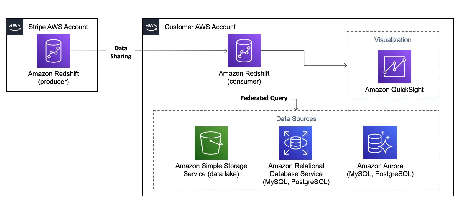
The following architecture diagram provides a quick overview of how data sharing works and how other AWS services can be used together. We dive deeper into different use cases in the following sections.

Accept datashares from Stripe

You can configure the solution in a few steps with no code necessary.

Once Stripe creates a datashare from the producer cluster and authorizes your AWS account, you can view this datashare on your Amazon Redshift console. You need to associate it with specific or all clusters in your AWS account as the consumer. Clusters can be specified by namespaces as globally unique identifiers. Next, you create a database from the datashare in order to start querying data.

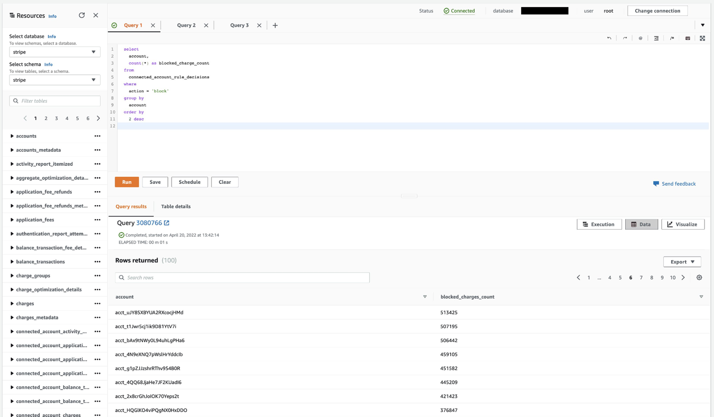
Query data from the consumer Amazon Redshift cluster

You can now access your Stripe data and schema directly from Amazon Redshift’s web-based query editor. This direct connection enables teams to pull accurate analysis of various functions of the business. For example:

  • Finance – “How does my cash flow change based on seasonality?”
  • Sales – “How many customers do we have in the US?”
  • Product – “How many active users do we have on each subscription plan?”
  • Sales operations – “Which customers haven’t paid their invoices?”

The following screenshot shows an example in which the query editor displays the number of charges blocked per Stripe’s connected account.

Use federated queries

The modern data architecture of Amazon Redshift enables you to store data in purpose-built data stores based on specific use cases, and allows querying external databases on Amazon Relational Database Service (Amazon RDS) or datasets in an Amazon Simple Storage Service (Amazon S3) data lake without moving these datasets to Amazon Redshift clusters. You can drive deeper by incorporating data from Amazon RDS, or from an S3 data lake through Amazon Redshift Spectrum. This capability provides a native integration without requiring additional ETL jobs.

The following syntax allows you to create an external schema from an Amazon Aurora MySQL-Compatible Edition database to an Amazon Redshift cluster. Amazon Redshift assumes an AWS Identity and Access Management (IAM) role and uses AWS Secrets Manager to access external data stores. For more information and examples with other supported data stores, refer to Querying data with federated queries in Amazon Redshift.

CREATE EXTERNAL SCHEMA auroram
FROM MYSQL
DATABASE ‘example_database’ SCHEMA 'example_schema' -- schema is optional
URI ‘hostname’
IAM_ROLE ‘iam_role_arn’
SECRET_ARN ‘aws_secrets_manager_arn’; 

Coming back to Stripe Data Pipeline, now you can combine the data from an Aurora table and create further analysis. For example, you can correlate the trends of customer acquisition against sales campaign by region, so you can gain an understanding of the campaign effectiveness and make adjustment to marketing strategies.
Create visualizations and dashboards

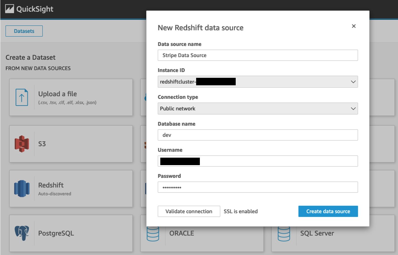
Now that your complete set of business data is accessible from Amazon Redshift, you can start to explore the data and create visualizations. Amazon QuickSight is a serverless BI service that allows you to easily connect to a data source, create analyses, publish dashboards, and share between teams. QuickSight seamlessly integrates with AWS services such as Amazon Redshift, Amazon S3, and many more.

The following screenshot illustrates how straightforward it is to connect an Amazon Redshift instance to QuickSight as a new data source.

The following screenshot is of a sample QuickSight dashboard pulling data from Amazon Redshift.

Key considerations

When using Stripe Data Pipeline, consider the following:

  • Instance type – This solution is available for all RA3 node types. If you run an existing DS2 or DC2 cluster, there are multiple options to migrate to RA3, including elastic resize, snapshot and restore, and classic resize. For more information, including an upgrade sizing reference between different node types, refer to Upgrading to RA3 node types.

  • RI migration – If you have Amazon Redshift Reserved Instances (RIs), you can use the RI migration feature to migrate the DS2 RI clusters to equivalent RA3 RI clusters as part of a cross-instance resize or cross-instance snapshot restore operation. The RA3 RI covering the new cluster will be the same cost and on the same calendar terms as the original DS2 RI for supported configurations.

  • Encryption – The consumer cluster must be encrypted as part of the enhanced security control for cross-account sharing. You can enable encryption at cluster creation time, or modify an unencrypted cluster with either AWS Key Management Service (AWS KMS) or AWS CloudHSM.
  • Federated queries – This capability works with external DB instances, including Amazon RDS for PostgreSQL, Amazon Aurora PostgreSQL-Compatible Edition, Amazon RDS for MySQL, and Aurora MySQL-Compatible Edition. You should also ensure that you have an Amazon Redshift cluster with a cluster maintenance version that supports federated queries.

Conclusion

In this post, we introduced Stripe Data Pipeline for Amazon Redshift and discussed options to further integrate with AWS services. Stripe Data Pipeline removes the need to build custom API integration or adopt a third-party ETL pipeline, making data accessible with a few clicks and with no code required. Businesses can automatically receive up-to-date data from Stripe in their data warehouse on AWS, reduce data silos, and extract deep insights to address business needs.

Check out Stripe Data Pipeline for more information about the solution and how to get started.


About the Authors

Jessica Ho is a Sr. Partner Solutions Architect at AWS supporting ISV partners who build business applications. She is passionate about creating differentiated solutions that promote cloud adoption. Outside of work, she enjoys spoiling her garden into a mini jungle.

Alexander Mahabir is a Sr. Partner Solutions Architect at AWS based in the D.C metropolitan area. Alex has over 16 year of experience building cloud, and on-premise solutions for small, medium, and large enterprises. Alex currently works with ISV partners in the Digital Customer Experience segment.

Coming June 2022: An updated Amazon QuickSight dashboard experience

Post Syndicated from Rushabh Vora original https://aws.amazon.com/blogs/big-data/coming-june-2022-an-updated-amazon-quicksight-dashboard-experience/

Starting June 30, 2022, Amazon QuickSight is introducing the new look and feel for your dashboards. In this post, we walk through the changes to expect with the new look. The new dashboard experience includes the following improvements:

  • Simplified toolbar
  • Discoverable visual menu
  • Polished controls, menu, and submenus
  • Non-blocking right pane for secondary experiences like filters, threshold alerts, and downloads

Simplified toolbar

The simplified toolbar experience offers updated icons for key actions for better visual clarity.

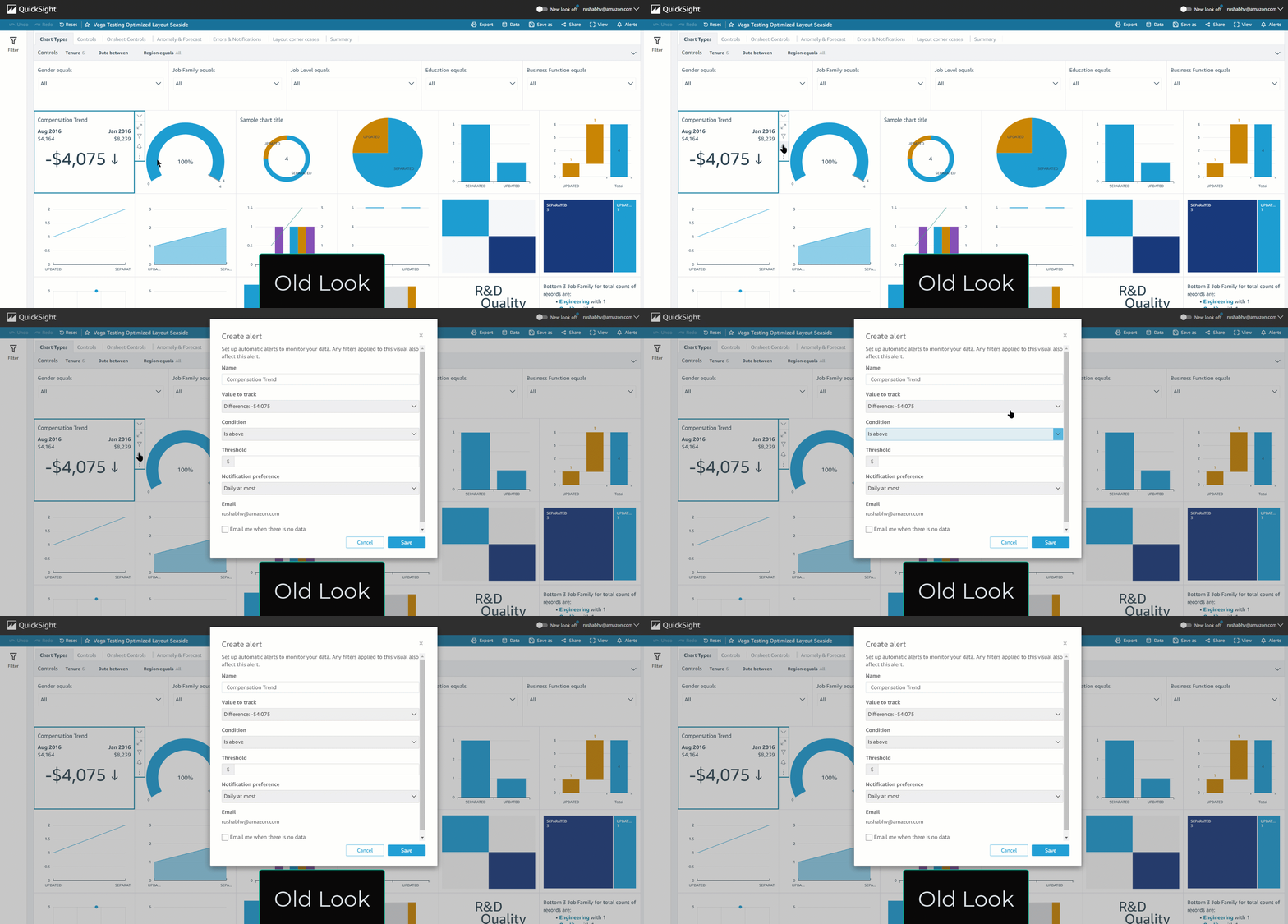
The following screenshot shows the old look.

screenshot shows the old look

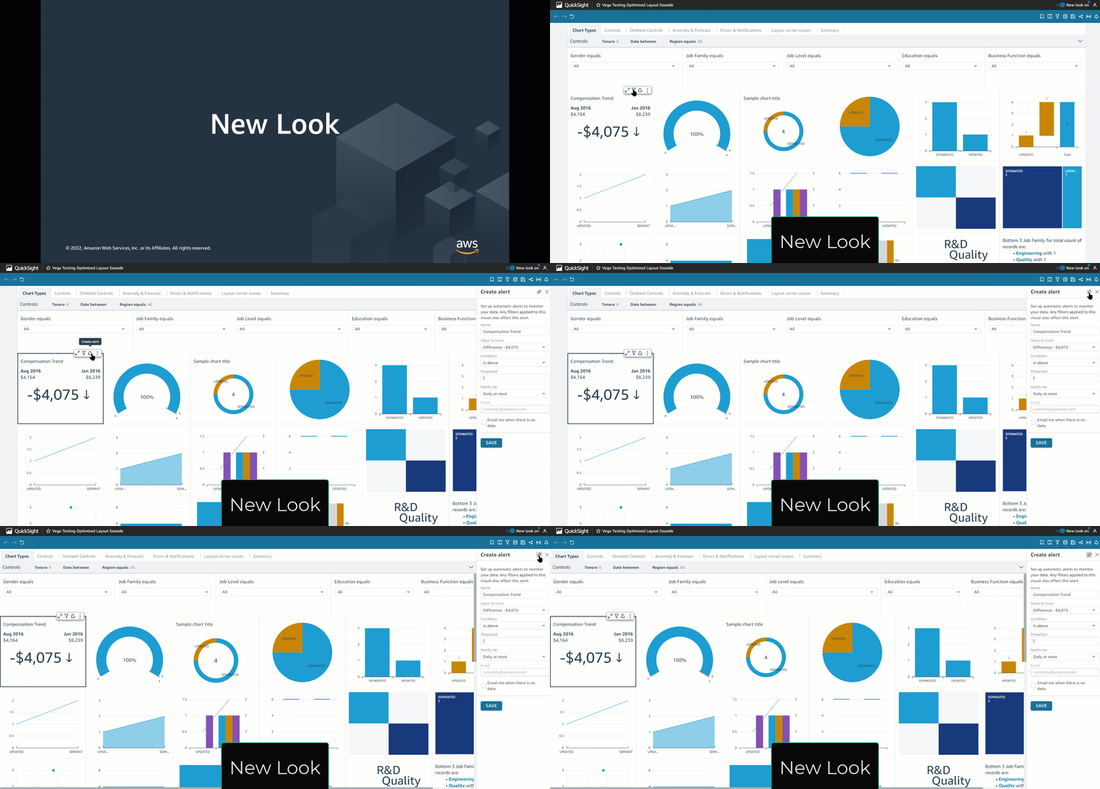
The following screenshot shows the new look with updated icons.

screenshot shows the new look with updated icons

Discoverable visual menu

The visual menu is visible on-hover to improve the discoverability of drills, export, and filter restatements.

To use the visual menu with the old version, you needed to select the visual.

visual menu with the old look, where you needed to select the visual

With the new look, you can view the menu by hovering over it.

With new look, you can view the menu by hovering over it

Polished controls, menu, and submenus

The new look features improved controls, menu, submenus, toast notifications, and other dashboard elements to provide more polished visual experience.

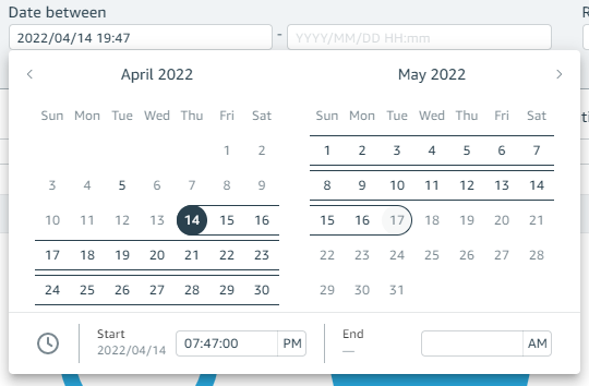
For example, the following screenshot shows the old look for calendar controls.

screenshot shows the old look for calendar controls

The following screenshot shows the new look.

screenshot shows the new look for calendar control

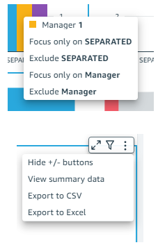
The following screenshot shows the old look for the menu and submenus.

screenshot shows the old look for the menu and submenus

The following screenshot shows the new look.

screenshot shows the new look for menu and submenus

Non-blocking right pane

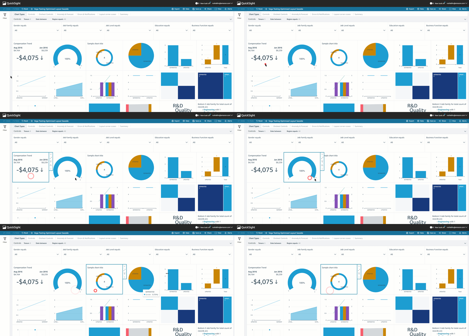
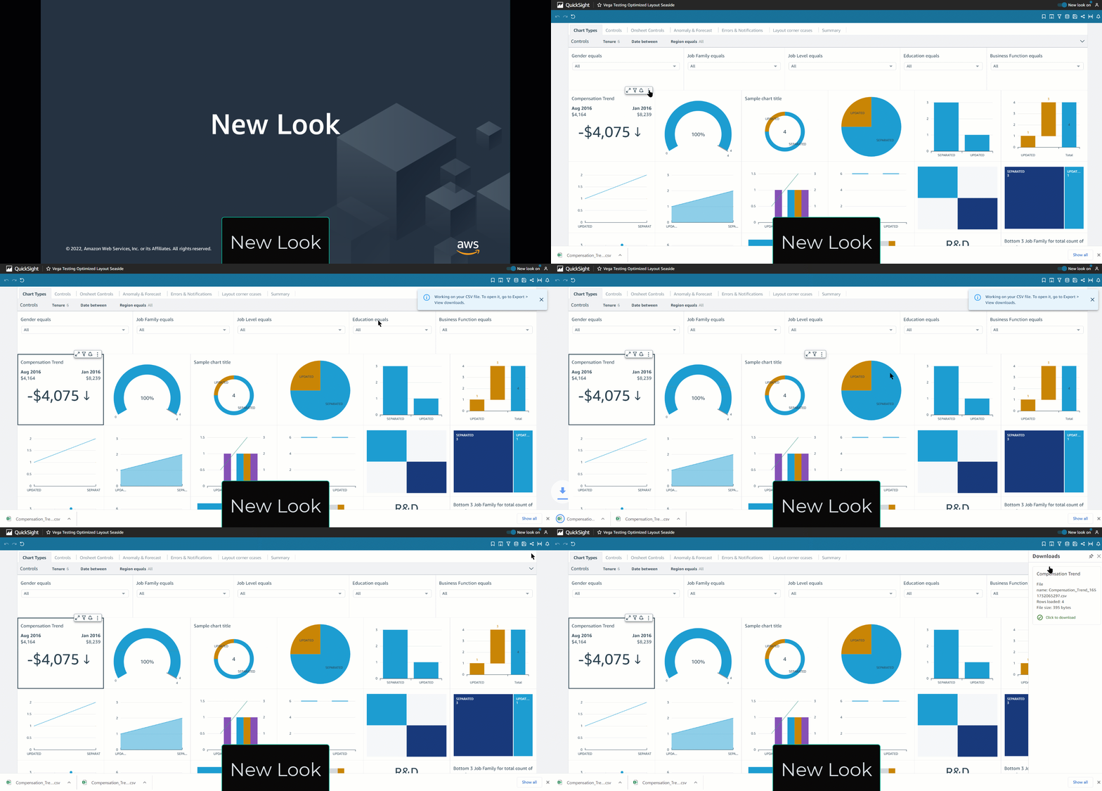
The new look features a non-blocking right pane for secondary experiences like filters, threshold alerts, and downloads, to improve focus on the content of the dashboard.‘

The following animation shows the old look for ad-hoc filtering.

animation shows the old look for ad-hoc filtering

The filters are now moved to the right pane.

animation shows the new look for ad-hoc filtering that is now moved to the right pane

The following animation shows the old look for creating threshold alerts.

animation shows the old look for creating threshold alerts

Threshold alert creation is now in the right pane.

animation shows the new look for creating threshold alerts, now moved to right pane

The following animation shows the old look for the downloading experience.

animation shows the old look for the downloading experience

The new look offers a downloads pane.

animation shows the new look for the downloading experience in the right pane

Summary

The new look for the QuickSight dashboard experience will be available starting June 30, 2022. If you have any questions or feedback, please reach out to us by leaving a comment.


About the Author

Rushabh Vora is a Senior Technical Product Manager for Amazon QuickSight, Amazon Web Service’s cloud-native, fully managed BI service. He is passionate about Data Visualization. Prior to QuickSight, he was working with Amazon Business as a Product Manager.

Use a linear learner algorithm in Amazon Redshift ML to solve regression and classification problems

Post Syndicated from Phil Bates original https://aws.amazon.com/blogs/big-data/use-a-linear-learner-algorithm-in-amazon-redshift-ml-to-solve-regression-and-classification-problems/

Amazon Redshift is the fastest, most widely used, fully managed, and petabyte-scale cloud data warehouse. Tens of thousands of customers use Amazon Redshift to process exabytes of data every day to power their analytics workloads. Amazon Redshift ML, powered by Amazon SageMaker, makes it easy for SQL users such as data analysts, data scientists, and database developers to create, train, and deploy machine learning (ML) models using familiar SQL commands and then use these models to make predictions on new data for use cases such as churn prediction, customer lifetime value prediction, and product recommendations. Redshift ML makes the model available as a SQL function within the Amazon Redshift data warehouse so you can easily use it in queries and reports. Customers across all verticals are using Redshift ML to derive better insights from their data. For example, Jobcase uses Redshift ML to recommend job search at scale. Magellan RX Management uses Redshift ML to predict drug therapeutic use conditions.

Amazon Redshift supports supervised learning, including regression, binary classification, multi-class classification, and unsupervised learning using K-Means. You can optionally specify XGBoost, MLP, and now linear learner model types, which are supervised learning algorithms used for solving either classification or regression problems, and provide a significant increase in speed over traditional hyperparameter optimization techniques. Amazon Redshift also supports bring-your-own-model to invoke remote SageMaker endpoints.

In this post, we show you how to use Redshift ML to solve regression and classification problems using the SageMaker linear learner algorithm, which explores different training objectives and chooses the best solution from a validation set.

Solution overview

We first solve a linear regression problem, followed by a multi-class classification problem.

The following table shows some common use cases and algorithms used.

Use Case Algorithm / Problem Type
Customer churn prediction Classification
Predict if a sales lead will close Classification
Fraud detection Classification
Price and revenue prediction Linear regression
Customer lifetime value prediction Linear regression

To use the linear learner algorithm, you need to provide inputs or columns representing dimensional values and also the label or target, which is the value you’re trying to predict. The linear learner algorithm trains many models in parallel, and automatically determines the most optimized model.

Prerequisites

To get started, we need an Amazon Redshift cluster or an Amazon Redshift Serverless endpoint and an AWS Identity and Access Management (IAM) role attached that provides access to SageMaker and permissions to an Amazon Simple Storage Service (Amazon S3) bucket.

For an introduction to Redshift ML and instructions on setting it up, see Create, train, and deploy machine learning models in Amazon Redshift using SQL with Amazon Redshift ML.

To create a simple cluster with a default IAM role, see Use the default IAM role in Amazon Redshift to simplify accessing other AWS services.

Use case 1: Linear regression

In this use case, we analyze the Abalone dataset and determine the relationship between the physical measurements and use that to determine the age of abalone. The age of abalone is determined by cutting the shell through the cone, staining it, and counting the number of rings through a microscope, which is a time-consuming task. We want to predict the age using different physical measurements, which is easier to measure. The age of abalone is (number of rings + 1.5) years.

Prepare the data

Load the Abalone dataset into Amazon Redshift using the following SQL. You can use the Amazon Redshift query editor v2 or your preferred SQL tool to run these commands.

To create the table, use the following commands:

create table abalone_dataset
( 
id INT IDENTITY(1,1),
Sex     CHAR(1),
Length float,
Diameter float,
Height float,
Whole  float,
Shucked  float,
Viscera  float,
Shell float,
Rings  integer   
); 

To load data into Amazon Redshift, use the following COPY command:

COPY abalone_dataset 
from 's3://redshift-ml-multiclass/abalone.csv' 
REGION 'us-east-1'
IAM_ROLE default
CSV IGNOREHEADER 1
NULL AS 'NULL'; 

To train the model, we use the abalone table and 80% of the data to train the model, and then test the accuracy of that model by seeing if it correctly predicts the age of ring label attribute on the remaining 20% of the data. Run the following command to create training and validation tables:

create table abalone_training as
  select * from abalone_dataset where mod(id,10) < 8 ; 

create table abalone_validation as
  select * from abalone_dataset where mod(id,10) >= 8; 

Create a model in Redshift ML

To create a model in Amazon Redshift, use the following command:

CREATE MODEL model_abalone_ring_prediction
FROM (
 SELECT   Sex ,
Length ,
Diameter ,
Height ,
Whole  ,
Shucked  ,
Viscera  ,
Shell,
Rings  as target_label
FROM abalone_training
) TARGET target_label
FUNCTION f_abalone_ring_prediction
IAM_ROLE default
MODEL_TYPE LINEAR_LEARNER 
PROBLEM_TYPE REGRESSION
OBJECTIVE 'MSE'
SETTINGS (
  S3_BUCKET '<your-s3-bucket>',
  MAX_RUNTIME 15000
  ); 

We define the following parameters in the CREATE MODEL statement:

  • Problem type – We use the linear learner problem type, which is newly added to extend upon typical linear models by training many models in parallel, in a computationally efficient manner.
  • Objective – We specified MSE (mean square error) as our objective, which is a common metric for evaluation of regression problems.
  • Max runtime –This parameter denotes how long the model training can run. Specifying a larger value may help create a better tuned model. The default value for this parameter is 5400 (90 minutes). For this example, we set it to 15000.

The preceding statement takes a few seconds to complete. It initiates an Amazon SageMaker Autopilot process in the background to automatically build, train, and tune the best ML model for the input data. It then uses Amazon SageMaker Neo to deploy that model locally in the Amazon Redshift cluster or Amazon Redshift Serverless as a user-defined function (UDF). You can use the SHOW MODEL command in Amazon Redshift to track the progress of your model creation, which should be in the READY state within the max_runtime parameter you defined while creating the model.

To check the status of the model, use the following command:

show model model_abalone_ring_prediction;

The following is the tabular outcome for the preceding command after model training was done. It took approximately 120 minutes to train the model.

Key Value
Model Name model_abalone_ring_prediction
Schema Name public
Owner awsuser
Creation Time Tue, 10.05.2022 19:42:33
Model State READY
validation:mse 4.082088
Estimated Cost 5.423719
. .
TRAINING DATA: .
Query SELECT SEX , LENGTH , DIAMETER , HEIGHT , WHOLE , SHUCKED , VISCERA , SHELL, RINGS AS TARGET_LABEL
. FROM ABALONE_TRAINING
Target Column TARGET_LABEL
. .
PARAMETERS: .
Model Type linear_learner
Problem Type Regression
Objective MSE
AutoML Job Name redshiftml-20220510194233380173
Function Name f_abalone_ring_prediction
Function Parameters sex length diameter height whole shucked viscera shell
Function Parameter Types bpchar float8 float8 float8 float8 float8 float8 float8
IAM Role default-aws-iam-role
S3 Bucket poc-generic-bkt
Max Runtime 15000

Model validation

We notice from the preceding table that the MSE for the training data is 4.08. Now let’s run the prediction query and validate the accuracy of the model on the testing and validation dataset:

select
ROUND(AVG(POWER(( tgt_label - predicted ),2)),2) mse
, ROUND(SQRT(AVG(POWER(( tgt_label - predicted ),2))),2) rmse
from 
(
SELECT   Sex ,
Length ,
Diameter ,
Height ,
Whole  ,
Shucked  ,
Viscera  ,
Shell,
Rings as tgt_label,
f_abalone_ring_prediction(Sex ,Length ,Diameter ,Height ,Whole  ,Shucked  ,Viscera  ,Shell) as predicted,
case when tgt_label = predicted then 1
      else 0 end as match,
  case when tgt_label  <> predicted then 1
    else 0 end as nonmatch
FROM abalone_validation
)t1 

The following is the outcome from the query:

mse rmse
5.08 2.25

The MSE value from the preceding query results indicates that our model is accurate enough to the actual values from our validation dataset.

We can also observe that Redshift ML is able to identify the right combination of features to come up with a usable prediction model. We can further check the impact of each attribute and its contribution and weightage in the model selection using the following command:

select explain_model ('model_abalone_ring_prediction')

The following is the outcome, where each attribute weightage is representative of its role in model decision-making:

{"explanations":
    {"kernel_shap":
      {"label0":
        {"expected_value":10.06938362121582,
          "global_shap_values":
          {
            "diameter":0.6897614190439705,
            "height":0.38391156156643987,
            "length":0.29646334630067408,
            "sex":0.5516722137411109,
            "shell":1.5679368167990147,
            "shucked":2.222549468867254,
            "viscera":0.2879883139361144,
            "whole":0.8085603201751219
            }
        }
       }
      }
      ,"version":"1.0"
    }

Use case 2: Multi-class classification

For this use case, we use the Covertype dataset (copyright Jock A. Blackard and Colorado State University), which contains information collected by the US Geological Survey and the US Forest Service about wilderness areas in northern Colorado. This has been downloaded to an S3 bucket to make it simple to create the model. You may want to download the dataset description. This dataset contains various measurements such as elevation, distance to waters and roadways, as well as the wilderness area designation and the soil type. Our ML task is to create a model to predict the cover type for a given area.

Prepare the data

To prepare the data for this model, you need to create and populate the table public.covertype_data in Amazon Redshift using the Covertype dataset. You may use the following SQL in Amazon Redshift query editor v2 or your preferred SQL tool:

CREATE TABLE public.covertype_data (
    elevation bigint ENCODE az64,
    aspect bigint ENCODE az64,
    slope bigint ENCODE az64,
    horizontal_distance_to_hydrology bigint ENCODE az64,
    vertical_distance_to_hydrology bigint ENCODE az64,
    horizontal_distance_to_roadways bigint ENCODE az64,
    hillshade_9am bigint ENCODE az64,
    hillshade_noon bigint ENCODE az64,
    hillshade_3pm bigint ENCODE az64,
    horizontal_distance_to_fire_points bigint ENCODE az64,
    wilderness_area1 bigint ENCODE az64,
    wilderness_area2 bigint ENCODE az64,
    wilderness_area3 bigint ENCODE az64,
    wilderness_area4 bigint ENCODE az64,
    soil_type1 bigint ENCODE az64,
    soil_type2 bigint ENCODE az64,
    soil_type3 bigint ENCODE az64,
    soil_type4 bigint ENCODE az64,
    soil_type5 bigint ENCODE az64,
    soil_type6 bigint ENCODE az64,
    soil_type7 bigint ENCODE az64,
    soil_type8 bigint ENCODE az64,
    soil_type9 bigint ENCODE az64,
    soil_type10 bigint ENCODE az64,
    soil_type11 bigint ENCODE az64,
    soil_type12 bigint ENCODE az64,
    soil_type13 bigint ENCODE az64,
    soil_type14 bigint ENCODE az64,
    soil_type15 bigint ENCODE az64,
    soil_type16 bigint ENCODE az64,
    soil_type17 bigint ENCODE az64,
    soil_type18 bigint ENCODE az64,
    soil_type19 bigint ENCODE az64,
    soil_type20 bigint ENCODE az64,
    soil_type21 bigint ENCODE az64,
    soil_type22 bigint ENCODE az64,
    soil_type23 bigint ENCODE az64,
    soil_type24 bigint ENCODE az64,
    soil_type25 bigint ENCODE az64,
    soil_type26 bigint ENCODE az64,
    soil_type27 bigint ENCODE az64,
    soil_type28 bigint ENCODE az64,
    soil_type29 bigint ENCODE az64,
    soil_type30 bigint ENCODE az64,
    soil_type31 bigint ENCODE az64,
    soil_type32 bigint ENCODE az64,
    soil_type33 bigint ENCODE az64,
    soil_type34 bigint ENCODE az64,
    soil_type35 bigint ENCODE az64,
    soil_type36 bigint ENCODE az64,
    soil_type37 bigint ENCODE az64,
    soil_type38 bigint ENCODE az64,
    soil_type39 bigint ENCODE az64,
    soil_type40 bigint ENCODE az64,
    cover_type bigint ENCODE az64 
)
DISTSTYLE AUTO;	


Copy public.covertype_data
From 's3://redshift-ml-multiclass/covtype.data.gz'
iam_role default 
gzip
delimiter ','
region 'us-east-1';

Now that our dataset is loaded, we run the following SQL statements to split the data into three sets for training (80%), validation (10%), and prediction (10%). Note that Redshift ML Autopilot automatically splits the data into training and validation, but by splitting it here, you’re able to verify the accuracy of your model.

To prepare the dataset, assign random values to split the data:

create table  public.covertype_data_prep  as
select a.*,
cast (random() * 80 as int) as data_group_id
from public.covertype_data a;

Use the following code for the training set:

Create table public.covertype_training as
Select * from public.covertype_data_prep
Where data_group_id < 80;

Use the following code for the validation set:

Create table public.covertype_validation as
Select * from public.covertype_data_prep
Where data_group_id between 80 and 89;

Use the following code for the test set:

Create table public.covertype_test as
Select * from public.covertype_data_prep
Where data_group_id > 89; 

Now that we have our datasets, it’s time to create the model.

Create a model in Redshift ML using linear learner

Run the following SQL command to create your model—note our target is cover_type and we use all the inputs from our training set:

CREATE  MODEL forest_cover_type_model
FROM (select Elevation, 
   Aspect,  
   Slope,  
   Horizontal_distance_to_hydrology,  
   Vertical_distance_to_hydrology,   
   Horizontal_distance_to_roadways,  
   HIllshade_9am,  
   Hillshade_noon,  
   Hillshade_3pm , 
   Horizontal_Distance_To_Fire_Points,  
   Wilderness_Area1,  
   Wilderness_Area2,   
   Wilderness_Area3,  
   Wilderness_Area4,  
   soil_type1,
   Soil_Type2,
   Soil_Type3, 
   Soil_Type4, 
   Soil_Type5,  
   Soil_Type6, 
   Soil_Type7,  
   Soil_Type8, 
   Soil_Type9, 
   Soil_Type10 , 
   Soil_Type11,  
   Soil_Type12 , 
   Soil_Type13 ,
   Soil_Type14, 
   Soil_Type15, 
   Soil_Type16,  
   Soil_Type17, 
   Soil_Type18,  
   Soil_Type19,  
   Soil_Type20,  
   Soil_Type21,  
   Soil_Type22,  
   Soil_Type23,  
   Soil_Type24, 
   Soil_Type25,  
   Soil_Type26, 
   Soil_Type27,  
   Soil_Type28,  
   Soil_Type29,  
   Soil_Type30,  
   Soil_Type31, 
   Soil_Type32, 
   Soil_Type33,  
   Soil_Type34, 
   Soil_Type36, 
   Soil_Type37,  
   Soil_Type38,  
   Soil_Type39, 
   Soil_Type40,
  Cover_type from public.covertype_training)
TARGET cover_type
FUNCTION predict_cover_type
IAM_ROLE default
MODEL_TYPE LINEAR_LEARNER              
PROBLEM_TYPE MULTICLASS_CLASSIFICATION 
 OBJECTIVE 'Accuracy'
SETTINGS (
  S3_BUCKET '<<your-amazon-s3-bucket-name>>’
, 
  S3_GARBAGE_COLLECT OFF,
  MAX_RUNTIME 9600
) ;

You can use the SHOW MODEL command to view the status of the model.

You can see that the model has an accuracy score of .730279 and is in the READY state. Now let’s run a query to do some validation of our own.

Model validation

Run the following SQL query against the validation table, using the function created by our model:

select 
 cast(sum(t1.match)as decimal(7,2)) as predicted_matches
,cast(sum(t1.nonmatch) as decimal(7,2)) as predicted_non_matches
,cast(sum(t1.match + t1.nonmatch) as decimal(7,2))  as total_predictions
,predicted_matches / total_predictions as pct_accuracy
from 
(select 
Elevation, 
   Aspect,  
   Slope,  
   Horizontal_distance_to_hydrology,  
   Vertical_distance_to_hydrology,   
   Horizontal_distance_to_roadways,  
   HIllshade_9am,  
   Hillshade_noon,  
   Hillshade_3pm , 
   Horizontal_Distance_To_Fire_Points,  
   Wilderness_Area1,  
   Wilderness_Area2,   
   Wilderness_Area3,  
   Wilderness_Area4,  
   soil_type1,
   Soil_Type2,
   Soil_Type3, 
   Soil_Type4, 
   Soil_Type5,  
   Soil_Type6, 
   Soil_Type7,  
   Soil_Type8, 
   Soil_Type9, 
   Soil_Type10 , 
   Soil_Type11,  
   Soil_Type12 , 
   Soil_Type13 ,
   Soil_Type14, 
   Soil_Type15, 
   Soil_Type16,  
   Soil_Type17, 
   Soil_Type18,  
   Soil_Type19,  
   Soil_Type20,  
   Soil_Type21,  
   Soil_Type22,  
   Soil_Type23,  
   Soil_Type24, 
   Soil_Type25,  
   Soil_Type26, 
   Soil_Type27,  
   Soil_Type28,  
   Soil_Type29,  
   Soil_Type30,  
   Soil_Type31, 
   Soil_Type32, 
   Soil_Type33,  
   Soil_Type34, 
   Soil_Type36, 
   Soil_Type37,  
   Soil_Type38,  
   Soil_Type39, 
   Soil_Type40,
   Cover_type as actual_cover_type,
   predict_cover_type( Elevation, 
   Aspect,  
   Slope,  
   Horizontal_distance_to_hydrology,  
   Vertical_distance_to_hydrology,   
   Horizontal_distance_to_roadways,  
   HIllshade_9am,  
   Hillshade_noon,  
   Hillshade_3pm , 
   Horizontal_Distance_To_Fire_Points,  
   Wilderness_Area1,  
   Wilderness_Area2,   
   Wilderness_Area3,  
   Wilderness_Area4,  
   soil_type1,
   Soil_Type2,
   Soil_Type3, 
   Soil_Type4, 
   Soil_Type5,  
   Soil_Type6, 
   Soil_Type7,  
   Soil_Type8, 
   Soil_Type9, 
   Soil_Type10 , 
   Soil_Type11,  
   Soil_Type12 , 
   Soil_Type13 ,
   Soil_Type14, 
   Soil_Type15, 
   Soil_Type16,  
   Soil_Type17, 
   Soil_Type18,  
   Soil_Type19,  
   Soil_Type20,  
   Soil_Type21,  
   Soil_Type22,  
   Soil_Type23,  
   Soil_Type24, 
   Soil_Type25,  
   Soil_Type26, 
   Soil_Type27,  
   Soil_Type28,  
   Soil_Type29,  
   Soil_Type30,  
   Soil_Type31, 
   Soil_Type32, 
   Soil_Type33,  
   Soil_Type34, 
   Soil_Type36, 
   Soil_Type37,  
   Soil_Type38,  
   Soil_Type39, 
   Soil_Type40) as predicted_cover_type,
case when actual_cover_type = predicted_cover_type then 1
      else 0 end as match,
  case when actual_cover_type <>  predicted_cover_type then 1
    else 0 end as nonmatch

from public.covertype_validation
) t1;

You can see that our accuracy is very close to our score from the SHOW MODEL output.

Run a prediction query

Let’s run a prediction query in Amazon Redshift ML using our function against our test dataset to see the most common class of cover type for the Neota Wilderness Area. We can denote this by checking wildnerness_area2 for a value of 1.

The dataset includes the following wilderness areas:

  1. Rawah Wilderness Area
  2. Neota Wilderness Area
  3. Comanche Peak Wilderness Area
  4. Cache la Poudre Wilderness Area

The cover types are in seven different classes:

  1. Spruce/Fir
  2. Lodgepole Pine
  3. Ponderosa Pine
  4. Cottonwood/Willow
  5. Aspen
  6. Douglas Fir
  7. Krummholz

There are also 40 different soil type definitions, which you can see in the dataset description, with a value of 0 or 1 to note if it’s applicable for a particular row. The following are a few example soil types:

  1. Cathedral family – Rock outcrop complex, extremely stony
  2. Vanet-Ratake families –Rocky outcrop complex, very stony
  3. Haploborolis family – Rock outcrop complex, rubbly
  4. Ratake family – Rock outcrop complex, rubbly
  5. Vanet family – Rock outcrop complex, rubbly
  6. Vanet-Wetmore families – Rock outcrop complex, stony
select t1. predicted_cover_type, count(*) 
from 
(     
select 
   Elevation, 
   Aspect,  
   Slope,  
   Horizontal_distance_to_hydrology,  
   Vertical_distance_to_hydrology,   
   Horizontal_distance_to_roadways,  
   HIllshade_9am,  
   Hillshade_noon,  
   Hillshade_3pm , 
   Horizontal_Distance_To_Fire_Points,  
   Wilderness_Area1,  
   Wilderness_Area2,   
   Wilderness_Area3,  
   Wilderness_Area4,  
   soil_type1,
   Soil_Type2,
   Soil_Type3, 
   Soil_Type4, 
   Soil_Type5,  
   Soil_Type6, 
   Soil_Type7,  
   Soil_Type8, 
   Soil_Type9, 
   Soil_Type10 , 
   Soil_Type11,  
   Soil_Type12 , 
   Soil_Type13 ,
   Soil_Type14, 
   Soil_Type15, 
   Soil_Type16,  
   Soil_Type17, 
   Soil_Type18,  
   Soil_Type19,  
   Soil_Type20,  
   Soil_Type21,  
   Soil_Type22,  
   Soil_Type23,  
   Soil_Type24, 
   Soil_Type25,  
   Soil_Type26, 
   Soil_Type27,  
   Soil_Type28,  
   Soil_Type29,  
   Soil_Type30,  
   Soil_Type31, 
   Soil_Type32, 
   Soil_Type33,  
   Soil_Type34, 
   Soil_Type36, 
   Soil_Type37,  
   Soil_Type38,  
   Soil_Type39, 
   Soil_Type40,
   predict_cover_type( Elevation, 
   Aspect,  
   Slope,  
   Horizontal_distance_to_hydrology,  
   Vertical_distance_to_hydrology,   
   Horizontal_distance_to_roadways,  
   HIllshade_9am,  
   Hillshade_noon,  
   Hillshade_3pm , 
   Horizontal_Distance_To_Fire_Points,  
   Wilderness_Area1,  
   Wilderness_Area2,   
   Wilderness_Area3,  
   Wilderness_Area4,  
   soil_type1,
   Soil_Type2,
   Soil_Type3, 
   Soil_Type4, 
   Soil_Type5,  
   Soil_Type6, 
   Soil_Type7,  
   Soil_Type8, 
   Soil_Type9, 
   Soil_Type10,
   Soil_Type11,  
   Soil_Type12, 
   Soil_Type13,
   Soil_Type14, 
   Soil_Type15, 
   Soil_Type16,  
   Soil_Type17, 
   Soil_Type18,  
   Soil_Type19,  
   Soil_Type20,  
   Soil_Type21,  
   Soil_Type22,  
   Soil_Type23,  
   Soil_Type24, 
   Soil_Type25,  
   Soil_Type26, 
   Soil_Type27,  
   Soil_Type28,  
   Soil_Type29,  
   Soil_Type30,  
   Soil_Type31, 
   Soil_Type32, 
   Soil_Type33,  
   Soil_Type34, 
   Soil_Type36, 
   Soil_Type37,  
   Soil_Type38,  
   Soil_Type39, 
   Soil_Type40) as predicted_cover_type 

from public.covertype_test
where wilderness_area2 = 1)
t1
group by 1;

Our model has predicted that the majority of cover is Spruce and Fir.

You can experiment with various combinations, such as determining which soil types are most likely to occur in a predicted cover type.

Conclusion

Redshift ML makes it easy for users of all levels to create, train, and tune models using a SQL interface. In this post, we walked you through how to use the linear learner algorithm to create regression and multi-class classification models. You can then use those models to make predictions using simple SQL commands and gain valuable insights.

To learn more about RedShift ML, visit Amazon Redshift ML.


About the Authors

Phil Bates is a Senior Analytics Specialist Solutions Architect at AWS with over 25 years of data warehouse experience.

Sohaib Katariwala is an Analytics Specialist Solutions Architect at AWS. He has 12+ years of experience helping organizations derive insights from their data.

Tahir Aziz is an Analytics Solution Architect at AWS. He has worked with building data warehouses and big data solutions for over 13 years. He loves to help customers design end-to-end analytics solutions on AWS. Outside of work, he enjoys traveling and cooking.

Jiayuan Chen is a Senior Software Development Engineer at AWS. He is passionate about designing and building data-intensive applications, and has been working in the areas of data lake, query engine, ingestion, and analytics. He keeps up with latest technologies and innovates things that spark joy.

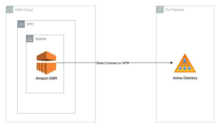
Debu Panda is a Senior Manager, Product Management at AWS, is an industry leader in analytics, application platform, and database technologies, and has more than 25 years of experience in the IT world. Debu has published numerous articles on analytics, enterprise Java, and databases and has presented at multiple conferences such as re:Invent, Oracle Open World, and Java One. He is lead author of the EJB 3 in Action (Manning Publications 2007, 2014) and Middleware Management (Packt).

Deep dive into Amazon EMR Kerberos authentication integrated with Microsoft Active Directory

Post Syndicated from Anandkumar Kaliaperumal original https://aws.amazon.com/blogs/big-data/deep-dive-into-amazon-emr-kerberos-authentication-integrated-with-microsoft-active-directory/

Many of our customers that use Amazon EMR as their big data platform need to integrate with their existing Microsoft Active Directory (AD) for user authentication. This integration requires the Kerberos daemon of Amazon EMR to establish a trusted connection with an AD domain, which involves a lot of moving pieces and can be difficult to get right.

This post describes what a one-way trust with Active Directory means, and how the commands work that are used in setting it up. We describe how DNS names, Kerberos realms, and AD domains are different, and the consequences of that for Amazon EMR security configuration and cluster one-way trust settings. We also discuss how you can’t use AWS Managed Microsoft AD for the Amazon EMR key distribution center (KDC) trust, and must either use an existing or new AD server.

AWS has already put out documentation and blog posts that cover some of this area, and this post is meant to complement them rather than replace them. As such, we recommend reading the following before continuing:

Is this the right architecture for you?

There are several options for authenticating Amazon EMR with Kerberos, and choosing the right approach will depend on your use case. For more information, refer to Kerberos architecture options. In this post, we cover the case where your users are already in your AD domain, and you want to use those identities to authorize actions in Amazon EMR. If you don’t already have an AD, or you want to extend an existing non-AD Kerberos realm, then one of the other options will be better suited. Don’t make more work for yourself than you have to!

Connecting to Active Directory

There are two goals when connecting Amazon EMR to AD:

  • Establish a one-way trust with from Kerberos to AD so that users working in Amazon EMR can use their AD credentials to access services. This requires ports 88, 464 (for Kerberos), and 139 (for LDAP) to be accessible from the EMR cluster.
  • Connect the EMR cluster with AD so that the servers making up the EMR cluster can be registered in the AD domain. This requires a user configured in the AD domain with sufficient privileges to make those registrations—typically called a bind user.

Types of Active Directory

The combination of the preceding requirements means that only an AD server can meet the goals. You can’t use AWS Managed Microsoft AD, nor Microsoft Azure AD. This leaves two options as the best practice.

Firstly, you can connect Amazon EMR directly to an existing AD server (whether on premises or in the cloud), as shown in the following diagram.

Alternatively, you can build a new AD server on Amazon Elastic Compute Cloud (Amazon EC2), add it to the existing corporate AD forest, and have Amazon EMR connect to this new cloud-based AD server (as shown in the following diagram).

Domains vs. realms

It is critical to understand which terms apply to which technology to avoid confusion.

Active Directory manages domains, which contain many registered entities like users and computers. They’re typically written in lowercase (for example, corp.mycompany.com) and look very similar to internet domains. They don’t necessarily have to resolve to an IP address, but they typically do.

Kerberos uses realms for a similar concept, and its registered entities are referred to as principals. Realms are typically written in uppercase, and often use a naming style that looks like an internet domain except for the case (for example, EMR.MYCOMPANY.COM). They don’t need to resolve to an IP address and typically do not.

When configuring the realm for an EMR cluster’s Kerberos daemon, the name is completely arbitrary. It serves as a namespace for the principals defined within it, but it doesn’t have to match the domain names of the instances in your EMR cluster. For example, if the private DNS names of your EC2 machines use the default ec2.internal domain, your EMR realm name doesn’t have to be ec2.internal; it could be mykerberosrealm or anything you like.

Bind user

A bind user has to be created in Active Directory with the permission to register (“bind”) EMR computers into the AD domain. Amazon EMR registers these computers under CN=Computers.

The Kerberos principals that Amazon EMR creates for use with the components of Hadoop are strictly local to the Amazon EMR Kerberos installation—they’re not registered in the AD domain.

DNS

The EMR Kerberos daemon has to be able to resolve the DNS name of your AD server in order to establish the trust between them. If those DNS domains are managed in your corporate DNS servers, you need Amazon Route 53 forwarders to your corporate DNS servers for Amazon EMR to resolve them. Because the trust is only one-way, the AD server doesn’t need to be able to resolve the internal DNS names of the EMR cluster nodes.

Establish trust

The trust that you need to establish from Amazon EMR to AD only needs to be one-way (Amazon EMR trusts AD), not two-way (they trust each other). To establish the one-way trust, use the ksetup and netdom utilities on the command line of the AD machine. The recommended encryption type attribute (SetEncTypeAttr) for the domain is an AES-256 cipher. The following code uses the example of the EMR Kerberos realm EMR.MYCOMPANY.COM and the AD domain corp.mycompany.com:

C:\Users\Administrator> ksetup /addkdc EMR.MYCOMPANY.COM
C:\Users\Administrator> netdom trust EMR.MYCOMPANY.COM /Domain:corp.mycompany.com /add /realm /passwordt:MyVeryStrongPassword
C:\Users\Administrator> ksetup /SetEncTypeAttr EMR.MYCOMPANY.COM AES256-CTS-HMAC-SHA1-96

In the first ksetup command, you don’t need to provide the fully qualified domain name of the cluster KDC as a final argument. That is only needed for a two-way trust, and is optional in a one-way trust.

Amazon EMR security configuration

Before you start the EMR cluster, you must create a security configuration that contains the details of the AD server and domain to which you’re connecting. The following screenshot shows an example of that configuration.

These fields are case-sensitive, so make sure that you enter everything correctly. Note that the domain and realm in this configuration both refer to the AD server, and not to the EMR cluster! Because AD can act as a Kerberos daemon as well as Active Directory, both of those fields are configured here. In both cases, however, they refer to the AD server and not the EMR cluster’s Kerberos domain.

Amazon EMR security options when starting a cluster

When you start an EMR cluster, you configure the security options as shown in the following screenshot.

Here you use the security configuration you just created, and specify the details of the EMR Kerberos realm as well as the parameters needed to establish the trust with the AD domain in the security configuration. You provide information for the following fields:

  • Realm – The Kerberos realm you specify is entirely up to you, but must be the same as the one you used when establishing the trust on the AD machine.
  • KDC admin password – This isn’t used anywhere else in the cluster configuration, so you can set it to something unique and secure specifically for this cluster. It’s only needed for any future management of the cluster-dedicated KDC.
  • Cross-realm trust principal password – This is the password you set with the netdom command.
  • Active Directory domain join user –This is the bind user your AD admin created.
  • Active Directory domain join password – This is the password for the bind user from AD.

Clean up

When you’re done testing this solution, remember to clean up the resources. If you used the CloudFormation templates to create the resources, then use the AWS CloudFormation console to delete the stack. Alternatively, you can use the AWS Command Line Interface (AWS CLI) or SDKs. For instructions, refer to Deleting a stack. Deleting a stack also deletes the resources created by that stack.

If one of your stacks doesn’t delete, make sure that there are no dependencies on the resources created by that stack. For example, if you deployed an Amazon VPC using AWS CloudFormation and then deployed a domain controller into that VPC using a different CloudFormation stack, you must first delete the domain controller stack before you can delete the VPC stack.

Conclusion

The steps in this post walked you through creating the trust between Amazon EMR’s Kerberos daemon and an Active Directory domain. We hope that this has demystified the process and makes it easy for you to create secure, AD-integrated EMR clusters in the future.


About the Authors

Anandkumar Kaliaperumal is a Senior Data Architect with the Professional Services SDT, where he focuses on helping customers with their Hadoop and data lake migrations. He lives with his growing family in Dallas.

Bharath Kumar Boggarapu is a Data Architect at AWS Professional Services with expertise in big data technologies. He is passionate about helping customers build performant and robust data-driven solutions and realize their data and analytics potential. His areas of interests are open-source frameworks, automation, and data architecting. In his free time, he loves to spend time with family, play tennis, and travel.


Oliver Meyn was a Senior Data Architect in the Canadian Professional Services Shared Delivery Team, where he helped customers with migrating their data and workflows to AWS. He lives in Toronto with his family and far too many bicycles.

Federate single sign-on access to Amazon Redshift query editor v2 with Okta

Post Syndicated from Sumeet Joshi original https://aws.amazon.com/blogs/big-data/federate-single-sign-on-access-to-amazon-redshift-query-editor-v2-with-okta/

Amazon Redshift query editor v2 is a web-based SQL client application that you can use to author and run queries on your Amazon Redshift data warehouse. You can visualize query results with charts and collaborate by sharing queries with members of your team. You can use query editor v2 to create databases, schemas, tables, and load data from Amazon Simple Storage Service (Amazon S3) using the COPY command or by using a wizard. You can browse multiple databases and run queries on your Amazon Redshift data warehouse or data lake, or run federated queries to operational databases such as Amazon Aurora. Because it’s a managed SQL editor in your browser and it’s integrated with your single sign-on (SSO) provider, Amazon Redshift query editor v2 reduces the number of steps to the first query so you gain insights faster.

Amazon Redshift query editor v2 integration with your identity provider (IdP) automatically redirects the user’s browser to the query editor v2 console instead of Amazon Redshift console. This enables your users to easily access Amazon Redshift clusters through query editor v2 using federated credentials without managing database users and passwords.

In this post, we focus on Okta as the IdP and illustrate how to set up your Okta application and AWS Identity and Access Management (IAM) permissions. We also demonstrate how you can limit the access for your users to use only query editor v2 without giving them access to perform any admin functions on the AWS Management Console.

Solution overview

The high-level steps in this post are as follows:

  1. Set up Okta, which contains your users organized into logical groups and AWS account federation application.
  2. Set up two IAM roles: one that establishes a trust relationship between your IdP and AWS, and a second role that Okta uses to access Amazon Redshift.
  3. Complete Okta advanced configuration:
    1. Finalize the Okta configuration by inputting the roles that you just created.
    2. Define a default relay state to direct users to Amazon Redshift query editor v2 after successful SAML authentication.
    3. Configure the SAML PrincipalTagAttribute. This element allows you to pass attributes as session tags in the SAML assertion. For more information about session tags, see Passing session tags in AWS STS.
  4. Set up Amazon Redshift database groups:
    1. Create groups within the Amazon Redshift database to match the Okta groups.
    2. Authorize these groups to access certain schemas and tables.
    3. Access Amazon Redshift query editor v2 using your enterprise credentials and query your Amazon Redshift database.
  5. Sign in to your Okta account and access the application assigned to you. The application directs you to Amazon Redshift query editor v2 using federated login.
  6. Access and query your Amazon Redshift database.

Prerequisites

This post assumes that you have the following prerequisites:

Set up Okta

First, we set up the Okta application and create users and groups. Complete the following steps:

  1. Log in to your Okta admin console using the URL https://<prefix>-admin.okta.com/admin/dashboard, where <prefix> is specific to your account and was created at account setup.
  2. On the admin console, choose Admin.
  3. Under Directory in the navigation pane, choose People.
  4. To add users, choose Add person.
    The following screenshot shows the users that we created.
  5. To add groups into Okta, choose Groups in the navigation pane, then choose Add group.
    The following screenshot shows two groups that we created. We added Jane to analyst_users and Mike to bi_users.
  6. Under Applications in the navigation pane, choose Applications and choose Browse App Catalog.
  7. Search for AWS Account Federation and choose Add.
  8. After you add the application, choose AWS Account Federation.
  9. Leave the values in General Settings at their default and choose Next.
  10. Under Sign-On Options, select SAML 2.0.
  11. Choose the Identity Provider metadata link to download the metadata file in .xml format.

Configure IAM roles

Next, you set up an IAM role that establishes a trust relationship between the IdP and AWS. You also create an IAM role that Okta uses to access Amazon Redshift query editor v2.

  1. On the IAM console, under Access management in the navigation pane, choose Identity providers.
  2. Choose Add provider.
  3. For Provider type¸ select SAML.
  4. For Provider name¸ enter a name.
  5. Choose Choose file and upload the metadata file you downloaded.
  6. Choose Add provider.

    Now you create the IAM SAML 2.0 federation role.
  7. On the IAM console, choose Roles in the navigation pane.
  8. Choose Create role.
  9. For Trusted entity type, select SAML 2.0 federation.
  10. For SAML 2.0-based provider, choose the IdP you created in the previous step.
  11. Select Allow programmatic and AWS Management Console access.
  12. Choose Next and then choose Create Policy.

Amazon Redshift query editor v2 provides multiple managed policies to access the query editor. For a list of managed policies, refer to Configuring your AWS account. The managed policy enables you to limit the access for your users to use only query editor v2 without giving them access to perform any admin functions on the console. For this post, we use the AmazonRedshiftQueryEditorV2ReadSharing managed policy and create a custom policy.

In the following code, provide your Region, account, and cluster parameters to grant access to Amazon Redshift to get cluster credentials, create users, and allow users to join groups:

{
    "Version": "2012-10-17",
    "Statement": [
        {
            "Sid": "RedshiftClusterPermissions",
            "Effect": "Allow",
            "Action": [
                "redshift:GetClusterCredentials",
                "redshift:CreateClusterUser",
                "redshift:JoinGroup"
            ],
            "Resource": [
                "arn:aws:redshift:<region>:<account>:cluster:<cluster>,                 
                "arn:aws:redshift:<region>:<account>:dbuser:<cluster>/${aws:PrincipalTag/RedshiftDbUser}",
                "arn:aws:redshift:<region>:<account>:dbgroup:<cluster>/analyst_users",
                "arn:aws:redshift:<region>:<account>:dbgroup:<cluster>/bi_users",
                "arn:aws:redshift:<region>:<account>:dbname:<cluster>/${redshift:DBName}"
            ]
        }
    ]
}

The group membership lasts only for the duration of the user session. Additionally, there is no CreateGroup permission because groups need to be manually created and granted DB privileges.

  1. Attach the policy you created to the role.
    The following screenshot shows the summary page for the role.
  2. Modify the trust relationships for your role and add sts:TagSession permission.
    When using session tags, trust policies for all roles connected to the IdP passing tags must have the sts:TagSession permission. For roles without this permission in the trust policy, the AssumeRole operation fails.
  3. Choose Update policy.

Set up Okta advanced configuration

In this section, you finalize the Okta configuration by adding the IAM roles that you just created. You set up SAML PrincipalTag attributes such as RedshiftDbUser and RedshiftDbGroups, which are passed in the SAML assertion to federate the access to Amazon Redshift query editor v2. You also define a default relay state, which is the URL that users are directed to after a successful authentication through SAML.

  1. In your Okta account, open the AWS Account Federation app.
  2. On the Sign On tab, set Default Relay State to the query editor URL, using the format https://<region>.console.aws.amazon.com/sqlworkbench/home. For this post, we use https://eu-west-1.console.aws.amazon.com/sqlworkbench/home.
  3. Choose Attributes and set up the following attribute mappings:
    1. Set the DB user using PrincipalTag:RedshiftDbUser. This uses the user name in the directory. This is a required tag and defines the database user that is used by query editor v2.
    2. Set the DB groups using PrincipalTag:RedshiftDbGroups. This uses the Okta groups to fill the principal tags. Its value must be a colon-separated list.
    3. Set the transitive keys using TransitiveTagKeys. This prevents users from changing the session tags in case of role chaining.

These tags are forwarded to the redshift:GetClusterCredentials API to get credentials for your cluster. The following table summarizes their attribute configuration.

Name Name Format Value
https://aws.amazon.com/SAML/Attributes/PrincipalTag:RedshiftDbUser Unspecified user.username
https://aws.amazon.com/SAML/Attributes/PrincipalTag:RedshiftDbGroups Unspecified String.join(“:”, isMemberOfGroupName(“analyst_users”) ? ‘analyst_users’ : ”, isMemberOfGroupName(“bi_users”) ? ‘bi_users’ : ”)
https://aws.amazon.com/SAML/Attributes/TransitiveTagKeys Unspecified Arrays.flatten(“RedshiftDbUser”, “RedshiftDbGroups”)

  1. Under Advanced Sign-on Settings¸ select Use Group Mapping.
  2. Enter the IdP and IAM role ARNs, which are globally unique, and make sure that Okta is directed to your AWS account.
  3. Authorize users to use the AWS Account Federation application by selecting their respective groups or individual user accounts. In this example, we authorized users by group.

Set up Amazon Redshift database groups

Next, you set up groups in the Amazon Redshift database to match the Okta groups. You also authorize these groups to access certain schemas and tables.

  1. Log in to your Amazon Redshift cluster with an admin account.
  2. Create groups that match the IdP group names, and grant the appropriate permissions to tables and schemas:
CREATE GROUP analyst_users;
CREATE GROUP bi_users;

ALTER DEFAULT PRIVILEGES IN SCHEMA sales_analysis
GRANT SELECT on TABLES to GROUP analyst_users;
GRANT USAGE on SCHEMA sales_analysis to GROUP analyst_users;
GRANT SELECT on ALL TABLES in SCHEMA sales_analysis to GROUP analyst_users;

ALTER DEFAULT PRIVILEGES IN SCHEMA sales_bi
GRANT SELECT on TABLES to GROUP bi_users;
GRANT USAGE on SCHEMA sales_bi to GROUP bi_users;
GRANT SELECT on ALL TABLES in SCHEMA sales_bi to GROUP bi_users;

In Okta, you created the user Jane and assigned Jane to the analyst_users group.

In the Amazon Redshift database, you created two database groups: analyst_users and bi_users.

When user Jane logs in via federated authentication to Amazon Redshift using query editor v2, the user is created if it doesn’t already exist and the analyst_users database group is assumed. The user Jane can query tables only in sales_analysis schema.

Because user Jane isn’t part of the bi_users group, when they try to access the sales_bi schema, they get a permission denied error.

The following diagram illustrates this configuration.

Access Amazon Redshift query editor v2

Now you’re ready to connect to your Amazon Redshift cluster using Amazon Redshift query editor v2 using federated login. Log in to your Okta account with your user credentials and under My Apps¸ choose Amazon Redshift Query Editor V2.

You’re redirected to the Amazon Redshift query editor v2 URL that you specified as the default relay state.

Connect to an Amazon Redshift database and run queries

Now let’s set up the connection to your Amazon Redshift cluster.

  1. In the query editor, choose your cluster (right-click) and choose Create connection.
  2. For Database, enter a name.
  3. For Authentication, select Federated user.
    The user name is prepopulated with your federated login information.
  4. Choose Create connection.

When you’re connected to your Amazon Redshift database, you can verify the connection details, as shown in the following screenshot. Notice the session-level group association as per the group assignment in your Okta application configuration. In this case, user Jane is assigned to the analyst_users group.

This user has access to SELECT all tables in the sales_analysis schema and no access to the sales_bi schema. You can run the following statements to test your access.

The following screenshot shows the results from a query to the sales_analysis.store_sales_us table.

When user Jane tries to access the tables in the sales_bi schema, they get a permission denied error.

Summary

In this post, we demonstrated how to federate SSO access to Amazon Redshift query editor v2 using Okta as your IdP. We showed how to set up Okta, set different PrinicpalTag attributes for query editor v2, and pass group memberships defined in your Okta IdP to your Amazon Redshift cluster. We showed how to log in to Amazon Redshift query editor v2 using federated login and validate the configuration by running a few queries. This solution allows you to control access to Amazon Redshift database objects, and your users can easily access Amazon Redshift clusters through query editor v2 using federated credentials without managing database users and passwords.

If you have any feedback or questions, please leave them in the comments.


About the Authors

Sumeet Joshi is an Analytics Specialist Solutions Architect based out of New York. He specializes in building large-scale data warehousing solutions. He has over 16 years of experience in the data warehousing and analytical space.

Bhanu Pittampally is an Analytics Specialist Solutions Architect based out of Dallas. He specializes in building analytical solutions. His background is in data and analytics for over 14 years. His LinkedIn profile can be found here.

Erol Murtezaoglu, a Technical Product Manager at AWS, is an inquisitive and enthusiastic thinker with a drive for self-improvement and learning. He has a strong and proven technical background in software development and architecture, balanced with a drive to deliver commercially successful products. Erol highly values the process of understanding customer needs and problems, in order to deliver solutions that exceed expectations.

Yanis Telaoumaten is a Software Development Engineer at AWS. His passions are building reliable software and creating tools to allow other engineers to work more efficiently. In the past years, he worked on identity, security and reliability of Redshift services

Federate access to Amazon Redshift query editor V2 with Active Directory Federation Services (AD FS): Part 3

Post Syndicated from Sumeet Joshi original https://aws.amazon.com/blogs/big-data/federate-access-to-amazon-redshift-query-editor-v2-with-active-directory-federation-services-ad-fs-part-3/

In the first post of this series, Federate access to your Amazon Redshift cluster with Active Directory Federation Services (AD FS): Part 1, you set up Microsoft Active Directory Federation Services (AD FS) and Security Assertion Markup Language (SAML) based authentication and tested the SAML federation using a web browser.

In Part 2, you learned to set up an Amazon Redshift cluster and use federated authentication with AD FS to connect from a JDBC SQL client tool.

In this post, we walk through the steps to configure Amazon Redshift query editor v2 to work with AD FS federation SSO.

Organizations want to enable their end-users such as data analysts, data scientists, and database developers to use the query editor v2 to accelerate self-service analytics. Amazon Redshift query editor v2 lets users explore, analyze, and collaborate on data. You can use the query editor to create databases, schemas, tables, and load data from Amazon Simple Storage Service (Amazon S3) using the COPY command or by using a wizard. You can browse multiple databases and run queries on your Amazon Redshift data warehouse or data lake, or run federated queries to operational databases such as Amazon Aurora.

In this post, we show how you can use your corporate Active Directory (AD) and the SAML 2.0 AD FS identity provider (IdP) to enable your users to easily access Amazon Redshift clusters through query editor v2 using corporate user names without managing database users and passwords. We also demonstrate how you can limit the access for your users to use only the query editor without giving them access to perform any admin functions on the AWS Management Console.

Solution overview

After you follow the steps explained in Part 1, you set up a deep link for federated users via the SAML 2.0 RelayState parameter in AD FS. You use the user you set up in your AD in Part 1 (Bob) to authenticate using AD FS and control access to database objects based on the group the user is assigned to. You also test if user Bob is integrated with Amazon Redshift database groups as controlled in AD groups.

By the end of this post, you will have created a unique deep link that authenticates the user Bob using AD FS and redirects them directly to the query editor v2 console, where they’re authenticated using the federation SSO option.

The sign-in process is as follows:

  1. The user chooses a deep link that redirects to the IdP for authentication with the information about the destination (query editor v2, in our case) URL embedded in the RelayState parameter. The user enters their credentials on the login page.
  2. Your IdP (AD FS in the case) verifies the user’s identity in your organization.
  3. Your IdP generates a SAML authentication response that includes assertions that identify the user and attributes about the user. The IdP sends this response to the user’s browser.
  4. The user’s browser is redirected to the AWS Single Sign-On endpoint and posts the SAML assertion and the RelayState parameter.
  5. The endpoint calls the AssumeRoleWithSAML API action to request temporary credentials from the AWS Identity and Access Management (IAM) role specified in the SAML assertion and creates a query editor v2 console sign-in URL that uses those credentials. The IAM role trusts the SAML federation entity and also has a policy that has access to query editor V2. If the SAML authentication response includes attributes that map to multiple IAM roles, the user is first prompted to choose the role to use for access to the query editor v2 console. The sign-in URL is the one specified by the RelayState parameter.
  6. AWS sends the sign-in URL back to the user’s browser as a redirect.
  7. The user’s browser is redirected to the Amazon Redshift query editor v2 console defined by the RelayState parameter.

The following diagram illustrates this flow.

In this post, we walk you through the following steps:

  1. Set up the Sales group in AD and set up the PrincipalTag claim rules in AD FS.
  2. Update the IAM roles.
  3. Construct the SSO URL to authenticate and redirect users to the Amazon Redshift query editor v2 console.
  4. Set up Amazon Redshift database groups and permissions on the Amazon Redshift cluster.
  5. Set up Amazon Redshift query editor v2 to use federated authentication with AD FS to connect directly from the query editor interface.
  6. Query Amazon Redshift objects to validate your authorization.

Prerequisites

For this walkthrough, complete the following prerequisite steps:

  1. Create an Amazon Redshift cluster. For instructions, refer to Create a sample Amazon Redshift cluster or complete the steps in Part 2 of this series.
  2. Complete the steps in Part 1 to set up SAML federation with AD FS:
    1. Set up an AD domain controller using an AWS CloudFormation template on a Windows 2016 Amazon Elastic Compute Cloud (Amazon EC2) instance.
    2. Configure federation in AD FS.
    3. Configure AWS as the relying party with AD FS using an IAM SAML provider and SAML roles with an attached policy to allow access to the Amazon Redshift cluster.
    4. Configure claim rules.
    5. Test the SAML authentication using a web browser.
  3. Verify that your IdP supports RelayState and is enabled. If you’re using AD FS 2.0, you need to download and install either Update Rollup 3 or Update Rollup 2 from Microsoft to enable the RelayState parameter.

Configure AD and AD FS

After you configure your AD FS and AD services by following the instructions in Part 1, you can set up the following AD group and claim rules.

In this post, you use the user Bob to log in to Amazon Redshift and check if Bob can access the Sales and Marketing schemas on the Amazon Redshift cluster. To create the sales group and assign the user [email protected] to it, log in to your AD FS server (Amazon EC2 machine) that you created in Part 1 and use the Windows command tool to run the following command:

dsadd group "cn=RSDB-sales, cn=Users, dc=adfsredshift, dc=com" -members "cn=Bob, cn=Users, dc=adfsredshift, dc=com"

Now you’re ready to create your custom claim rules: PrincipalTag:RedshiftDbUser and PrincipalTag:RedshiftDbGroup.

PrincipalTag:RedshiftDbUser

The custom claim rule PrincipalTag:RedshiftDbUser is mapped to the universal principal name in AD FS. When a user authenticates through federated SSO, this claim rule is mapped to the user name. If user doesn’t exist in the Amazon Redshift database, then the user is automatically created. The auto create option is granted through an IAM policy that is attached to the IAM role. The CreateClusterUser permission allows for auto creation of the user (you set this up as part of Part 1 as a prerequisite).

Complete the following steps to create your custom claim rule:

    1. On the AD FS management console, choose Relying Party Trusts.
    2. Choose Edit Claim Issuance Policy.
    3. Choose Choose Rule Type.
    4. For Claim rule template, choose Send Claims Using a Custom Rule.
    5. Choose Next.
    6. For Claims rule name, enter RedshiftDbUser.
    7. Add the following custom rule:
      c:[Type == "http://schemas.microsoft.com/ws/2008/06/identity/claims/windowsaccountname", Issuer == "AD AUTHORITY"]
       => issue(store = "Active Directory", types = ("https://aws.amazon.com/SAML/Attributes/PrincipalTag:RedshiftDbUser"), query = ";userPrincipalName;{0}", param = c.Value);

    8. Choose Finish.
    9. Capture the claim rules sent in a SAML assertion response through your browser. For instructions, refer to How to view a SAML response in your browser for troubleshooting.

In my example, I use the following SAML attribute for the RedshiftDbUser PrincipalTag:

<Attribute Name="https://aws.amazon.com/SAML/Attributes/PrincipalTag:RedshiftDbUser"> <AttributeValue>[email protected]</AttributeValue> 
</Attribute>

PrincipalTag:RedshiftDbGroup

The custom claim rule PrincipalTag:RedshiftDbGroup is built out of AD groups that the user is a member of. This rule is mapped to the Amazon Redshift database groups. The AD groups and Amazon Redshift database group names should match. JoinGroup permission set in the IAM policy allows the user to assume a database group and is session based. If the user is mapped to multiple groups in the AD group, the SAML assertion response should send those groups in : separated values and not as multiple value claims. The following steps demonstrate how to send AD groups as : separated values.

In this example, the user Bob is assigned to the marketing and sales groups. The following code shows how to send multiple groups through the SAML response when the user is in multiple groups, and also how to handle the situation when a user doesn’t exist in any particular group.

  1. Follow the same steps as in the previous section to create the rule Marketing, using the following code for the custom rule:
    c:[Type == " http://temp/groups", Value =~ "RSDB-Marketing"] => add(Type = " http://temp/marketing", Value = c.Value);

  2. Create the rule MarketingNotExists using the following code:
    NOT EXISTS([Type == "http://temp/variable", Value =~ "RSDB-marketing"]) => add(Type = "http://temp/marketing", Value = ""); 

  3. Create the rule sales using the following code:
    c:[Type == " http://temp/groups", Value =~ "RSDB-sales"] => add(Type = " http://temp/marketing", Value = c.Value);

  4. Create the rule SalesNotExists using the following code:
    NOT EXISTS([Type == "http://temp/variable", Value =~ "RSDB-sales"])
     => add(Type = "http://temp/sales", Value = ""); 

  5. Create the rule RedshiftDbGroups using the following code:
    c:[Type == "http://temp/marketing"]
     && c2:[Type == "http://temp/sales"]
     => issue(Type = "https://aws.amazon.com/SAML/Attributes/PrincipalTag:RedshiftDbGroups", Value = c.Value + ":" + c2.Value);

The following screenshot shows the list of rules that I created in my AD FS. Note the number of rules and the order in which they’re positioned. We created rules 6–11 as part of this post.

If you see a similar SAML response for RedshiftDbGroups, your setup is good:

<Attribute Name="https://redshift.amazon.com/SAML/Attributes/PrincipalTag:RedshiftDbGroups"> <AttributeValue> marketing:sales</AttributeValue>

If a user doesn’t exist in one of the groups, an empty value is passed to the claim rule. For example, if user bob is removed from the marketing group, the SAML response for PrincipalTag:RedshiftDbGroup would be :sales.

Update IAM roles

In Part 1 of this series, you created two IAM roles: ADFZ-Dev and ADFZ-Production. These two roles aren’t yet set up with grants on the query editor. In this section, you update these roles with query editor permissions.

Amazon Redshift query editor v2 provides multiple managed policies to access the query editor. For a list of all the managed policies, refer to Configuring your AWS account. For this post, we attach the AmazonRedshiftQueryEditorV2ReadSharing managed policy to the roles.

  1. On the IAM console, choose Roles in the navigation pane.
  2. Choose the role ADFZ-Dev.
  3. Choose Add permissions and then Attach policies.
  4. Under Other permission policies, search for the AmazonRedshiftQueryEditorV2ReadSharing managed policy.
  5. Select the policy and choose Attach policies.
  6. Modify the trust relationships for your role and add sts:TagSession. While in role select Trust relationships and click on Edit trust policy.When using session tags, trust policies for all roles connected to the IdP passing tags must have the sts:TagSession permission. For roles without this permission in the trust policy, the AssumeRole operation fails.
  7. Choose Update policy.
  8. Repeat these steps to attach the AmazonRedshiftQueryEditorV2ReadSharing managed policy to the ADFZ-Production role.

Limiting User access only to Query Editor

If you would like to limit users only access Query Editor then  update the policy redshift-marketing that you have created in Part 1 blog post as below.

Note: once updated, users will lose admin privileges such as create cluster.

Replace the region, account, and cluster parameters. This custom policy grants access to Amazon Redshift to get cluster credentials, create users, and allow users to join groups.

{
    "Version": "2012-10-17",
    "Statement": [
        {
            "Sid": "RedshiftClusterPermissions",
            "Effect": "Allow",
            "Action": [
                "redshift:GetClusterCredentials",
                "redshift:CreateClusterUser",
                "redshift:JoinGroup"
            ],
            "Resource": [
                "arn:aws:redshift:<region>:<account>:cluster:<cluster>,
                "arn:aws:redshift:<region>:<account>:dbuser:<cluster>/${aws:PrincipalTag/RedshiftDbUser}",
                "arn:aws:redshift:<region>:<account>:dbgroup:<cluster>/marketing",
                "arn:aws:redshift:<region>:<account>:dbgroup:<cluster>/sales",
                "arn:aws:redshift:<region>:<account>:dbname:<cluster>/${redshift:DBName}"
            ]
        }
    ]
}

There are a few important things to note:

  1. The group membership lasts only for the duration of the user session.
  2. There is no CreateGroup permission because groups need to be manually created and granted DB privileges.

Generate the SSO destination URL as the Amazon Redshift query editor v2 console

In this step, you construct the sign-in URL for the AD FS IdP to redirect users to the Amazon Redshift query editor v2 console. For instructions, refer to How to Use SAML to Automatically Direct Federated Users to a Specific AWS Management Console Page.

To provide a full SSO experience for the end-users, the SAML response can include an optional parameter called RelayState. This parameter contains the destination URL.

Microsoft provides a tool to help generate these SSO URLs for AD FS called the AD FS 2.0 RelayState Generator.

To build this URL, you need three pieces of information:

  • IdP URL string – The string is in the format https://ADFSSERVER/adfs/ls/idpinitiatedsignon.aspx. For this post, we use https://EC2AMAZ-F9TJOIC.adfsredshift.com/adfs/ls/IdpInitiatedSignOn.aspx.
  • Relying party identifier – For AWS, this is urn:amazon:webservices.
  • Relay state or target app – This is the AWS Management Console URL you want your authenticated users redirect to. In this case, it’s https://eu-west-1.console.aws.amazon.com/sqlworkbench/home?. For this post, we use the eu-west-1 Region, but you can adjust this as needed.

I followed the instructions in How to Use SAML to Automatically Direct Federated Users to a Specific AWS Management Console Page and used the AD FS 2.0 RelayState Generator to generate the URL shown in the following screenshot.

The following is an example of the final URL that you use to get authenticated and also get redirected to Amazon Redshift query editor v2 (this URL won’t work in your setup because it has been created specifically for an AD FS server in my account): https://EC2AMAZ-F9TJOIC.adfsredshift.com/adfs/ls/IdpInitiatedSignOn.aspx?RelayState=RPID%3Durn%253Aamazon%253Awebservices%26RelayState%3Dhttps%253A%252F%252Feu-west-1.console.aws.amazon.com%252Fsqlworkbench%252Fhome%253Fregion%253Deu-west-1%2523%252Fclient

You can now save this URL and use it from anywhere you can reach your AD FS server. After you enter the URL in a browser, you first authenticate to AD FS, then you’re redirected to the Amazon Redshift query editor v2 console.

Set up DB groups on Amazon Redshift cluster

In this step, you set up your Amazon Redshift database group. This step is necessary because when the user is authenticated, they have to be part of an Amazon Redshift DB group with proper permissions set on a schema or table (or view).

In Active Directory, the user Bob is part of two groups: Sales and Marketing. In your Amazon Redshift database, you have three database groups: Sales, Marketing, and Finance.

When user Bob logs in via federated authentication, the user assumes the Sales and Marketing database groups, so this user can query tables in both the Sales and Marketing schemas. Because the user Bob isn’t part of the Finance group, when they try to access the Finance schema, they receive a permission denied error.

The following diagram illustrates this configuration.

Complete the following steps to set up your DB groups:

  1. Connect as awsuser (a superuser).
  2. Create three database groups:
    CREATE GROUP sales;
    CREATE GROUP marketing;
    CREATE GROUP finance;

  3. Create three schemas:
    CREATE SCHEMA sales;
    CREATE SCHEMA marketing;
    CREATE SCHEMA finance;

  4. Create a table in each schema:
    CREATE TABLE IF NOT EXISTS marketing.employee
    (
    	n_empkey INTEGER   
    	,n_name CHAR(25)   
    	,n_regionkey INTEGER   
    	,n_comment VARCHAR(152)   
    )
    DISTSTYLE AUTO
     SORTKEY (n_empkey);
    
    CREATE TABLE IF NOT EXISTS sales.employee_sales
    (
    	n_empkey INTEGER   
    	,n_name CHAR(25)   
    	,n_regionkey INTEGER   
    	,n_comment VARCHAR(152)   
    )
    DISTSTYLE AUTO
     SORTKEY (n_empkey);
    
    
    CREATE TABLE IF NOT EXISTS finance.accounts
    (
    	account_id INTEGER   
    	,account_name CHAR(25)   
    	 
    )
    DISTSTYLE AUTO
     SORTKEY (account_id);

  5. Insert sample data into the three tables:
    INSERT INTO marketing.employee
    VALUES(1, 'Bob', 0, 'Marketing');
    
    INSERT INTO sales.employee_sales
    VALUES(1, 'John', 0, 'Sales');
    
    INSERT INTO finance.accounts
    VALUES(1, 'online company');

  6. Validate the data is available in the tables:
    Select * from marketing.employee;
    Select * from sales.employee_sales;
    Select * from finance.accounts;

You can now set up appropriate privileges for the sales, finance, and marketing groups. Groups are collections of users who are all granted privileges associated with the group. You can use groups to assign privileges by job function. For example, you can create different groups for sales, administration, and support, and give the users in each group the appropriate access to the data they require for their work. You can grant or revoke privileges at the group level, and those changes apply to all members of the group, except for superusers.

  1. Enter the following SQL queries to grant access to all tables in the sales schema to the sales group, access to all tables in the marketing schema to the marketing group, and access to all tables in the finance schema to the finance group:
ALTER DEFAULT PRIVILEGES IN SCHEMA sales
GRANT SELECT on TABLES to GROUP sales;
GRANT USAGE on SCHEMA sales to GROUP sales;
GRANT SELECT on ALL TABLES in SCHEMA sales to GROUP sales;

ALTER DEFAULT PRIVILEGES IN SCHEMA marketing
GRANT SELECT on TABLES to GROUP marketing;
GRANT USAGE on SCHEMA marketing to GROUP marketing;
GRANT SELECT on ALL TABLES in SCHEMA marketing to GROUP marketing;

ALTER DEFAULT PRIVILEGES IN SCHEMA finance
GRANT SELECT on TABLES to GROUP finance;
GRANT USAGE on SCHEMA finance to GROUP finance;
GRANT SELECT on ALL TABLES in SCHEMA finance to GROUP finance;

Access Amazon Redshift query editor v2 through federated authentication

Now that you have completed your SAML integration, deep link setup, and DB groups and access rights configuration, you can set up Amazon Redshift query editor v2 to use federated authentication with AD FS to connect from directly from the query editor interface.

  1. Navigate to the deep link URL you created earlier.
    You’re redirected to the AD FS login page.
  2. Sign in as [email protected].
    For this post, I accessed this URL from an Amazon EC2 machine, but you can access it from any location where you can reach the AD FS IdP.
    After AD FS successfully authenticates you, it redirects to the AWS SSO endpoint and posts the SAML assertion and RelayState parameter. Because you configured two IAM roles on the AWS side, you’re prompted to select a role.
  3. Select a role (for this example, ADFZ-Dev) and choose Sign In.

    AWS sends the sign-in URL that is based on the RelayState value back to your browser as a redirect. Your browser is redirected to the query editor v2 console automatically.
  4. Right-click your Amazon Redshift cluster (for this post, redshift-cluster-1) and choose Edit connection.

    The value for User name is automatically populated, and Federated Access is automatically selected.
  5. Choose Edit connection to save the connection and log in to the database.

    After you’re successfully logged in, you can browse the database objects in the left pane.
  6. Test the connection by running the following query:
    select * from stv_sessions;

The following screenshot shows the output.

The output shows that the user [email protected] was authenticated using AD FS. The user also joined the marketing and Sales groups as enforced by the AD FS PrincipalTag:RedshiftDbGroups claim rule and the policy associated with the ADFZ-Dev role, which the user assumes during this session.

Run queries to validate authorization through federated groups

In this final step, you validate how the groups and membership configured in AD are seamlessly integrated with Amazon Redshift database groups.

Run the following query against the marketing and sales schema:

select * from marketing.employee;
select * from sales.employee_sales;

The following screenshots shows the output:

The preceding images show that AD user Bob is part of the AD group RSDB-marketing and RSDB-sales, which are mapped to the DB groups marketing and sales. These DB groups have select access to the schemas marketing and sales and all tables in those schemas. Therefore, the user can successfully query the tables.

To run a query against the finance schema, enter the following code:

select * from finance.accounts;

The following screenshot shows the output.

The output shows that Bob is only part of the AD groups RSDB-marketing and RSDB-sales. Due to the way the claim rule is set up, Bob doesn’t have access to the database group finance, and therefore the query returns with a permission denied error.

Clean up

To avoid incurring future charges, delete the resources by deleting the CloudFormation stack. This cleans up all the resources from your AWS account that you set up in Part 1.

Conclusion

In this post, we demonstrated how to set up an AD FS server, configure different PrincipalTag attributes used for Amazon Redshift query editor v2, and generate an SSO URL with the query editor as the destination location. You then connected to the Amazon Redshift DB cluster using a database user with administrator privileges to set up DB groups and permissions, and used a federated user authentication with AD FS to run several queries. This solution enables you to control access to your Amazon Redshift database objects by using AD groups and memberships seamlessly.

If you have any feedback or questions, please leave them in the comments.


About the Authors

Sumeet Joshi is an Analytics Specialist Solutions Architect based out of New York. He specializes in building large-scale data warehousing solutions. He has over 16 years of experience in the data warehousing and analytical space.

Bhanu Pittampally is an Analytics Specialist Solutions Architect based out of Dallas. He specializes in building analytical solutions. His background is in data and analytics for over 14 years. His LinkedIn profile can be found here.

Erol Murtezaoglu, a Technical Product Manager at AWS, is an inquisitive and enthusiastic thinker with a drive for self-improvement and learning. He has a strong and proven technical background in software development and architecture, balanced with a drive to deliver commercially successful products. Erol highly values the process of understanding customer needs and problems, in order to deliver solutions that exceed expectations.

Yanis Telaoumaten is a Software Development Engineer at AWS. His passions are building reliable software and creating tools to allow other engineers to work more efficiently. In the past years, he worked on identity, security and reliability of Redshift services

How Paytm modernized their data pipeline using Amazon EMR

Post Syndicated from Rajat Bhardwaj original https://aws.amazon.com/blogs/big-data/how-paytm-modernized-their-data-pipeline-using-amazon-emr/

This post was co-written by Rajat Bhardwaj, Senior Technical Account Manager at AWS and Kunal Upadhyay, General Manager at Paytm.

Paytm is India’s leading payment platform, pioneering the digital payment era in India with 130 million active users. Paytm operates multiple lines of business, including banking, digital payments, bill recharges, e-wallet, stocks, insurance, lending and mobile gaming. At Paytm, the Central Data Platform team is responsible for turning disparate data from multiple business units into insights and actions for their executive management and merchants, who are small, medium or large business entities accepting payments from the Paytm platforms.

The Data Platform team modernized their legacy data pipeline with AWS services. The data pipeline collects data from different sources and runs analytical jobs, generating approximately 250K reports per day, which are consumed by Paytm executives and merchants. The legacy data pipeline was set up on premises using a proprietary solution and didn’t utilize the open-source Hadoop stack components such as Spark or Hive. This legacy setup was resource-intensive, having high CPU and I/O requirements. Analytical jobs took approximately 8–10 hours to complete, which often led to Service Level Agreements (SLA) breaches. The legacy solution was also prone to outages due to higher than expected hardware resource consumption. Its hardware and software limitations impacted the ability of the system to scale during peak load. Data models used in the legacy setup processed the entire data every time, which led to an increased processing time.

In this post, we demonstrate how the Paytm Central Data Platform team migrated their data pipeline to AWS and modernized it using Amazon EMR, Amazon Simple Storage Service (Amazon S3) and underlying AWS Cloud infrastructure along with Apache Spark. We optimized the hardware usage and reduced the data analytical processing, resulting in shorter turnaround time to generate insightful reports, all while maintaining operational stability and scale irrespective of the size of daily ingested data.

Overview of solution

The key to modernizing a data pipeline is to adopt an optimal incremental approach, which helps reduce the end-to-end cycle to analyze the data and get meaningful insights from it. To achieve this state, it’s vital to ingest incremental data in the pipeline, process delta records and reduce the analytical processing time. We configured the data sources to inherit the unchanged records and tuned the Spark jobs to only analyze the newly inserted or updated records. We used temporal data columns to store the incremental datasets until they’re processed. Data intensive Spark jobs are configured in incremental on-demand deduplicating mode to process the data. This helps to eliminate redundant data tuples from the data lake and reduces the total data volume, which saves compute and storage capacity. We also optimized the scanning of raw tables to restrict the scans to only the changed record set which reduced scanning time by approximately 90%. Incremental data processing also helps to reduce the total processing time.

At the time of this writing, the existing data pipeline has been operationally stable for 2 years. Although this modernization was vital, there is a risk of an operational outage while the changes are being implemented. Data skewing needs to be handled in the new system by an appropriate scaling strategy. Zero downtime is expected from the stakeholders because the reports generated from this system are vital for Paytm’s CXO, executive management and merchants on a daily basis.

The following diagram illustrates the data pipeline architecture.

Benefits of the solution

The Paytm Central Data Office team, comprised of 10 engineers, worked with the AWS team to modernize the data pipeline. The team worked for approximately 4 months to complete this modernization and migration project.

Modernizing the data pipeline with Amazon EMR 6.3 helped efficiently scale the system at a lower cost. Amazon EMR managed scaling helped reduce the scale-in and scale-out time and increase the usage of Amazon Elastic Compute Cloud (Amazon EC2) Spot Instances for running the Spark jobs. Paytm is now able to utilize a Spot to On-Demand ratio of 80:20, resulting in higher cost savings. Amazon EMR managed scaling also helped automatically scale the EMR cluster based on YARN memory usage with the desired type of EC2 instances. This approach eliminates the need to configure multiple Amazon EMR scaling policies tied to specific types of EC2 instances as per the compute requirements for running the Spark jobs.

In the following sections, we walk through the key tasks to modernize the data pipeline.

Migrate over 400 TB of data from the legacy storage to Amazon S3

Paytm team built a proprietary data migration application with the open-source AWS SDK for Java for Amazon S3 using the Scala programming language. This application can connect with multiple cloud providers , on-premises data centers and migrate the data to a central data lake built on Amazon S3.

Modernize the transformation jobs for over 40 data flows

Data flows are defined in the system for ingesting raw data, preprocessing the data and aggregating the data that is used by the analytical jobs for report generation. Data flows are developed using Scala programming language on Apache Spark. We use an Azkaban batch workflow job scheduler for ordering and tracking the Spark job runs. Workflows are created on Amazon EMR to schedule these Spark jobs multiple times during a day. We also implemented Spark optimizations to improve the operational efficiency for these jobs. We use Spark broadcast joins to handle the data skewness, which can otherwise lead to data spillage, resulting in extra storage needs. We also tuned the Spark jobs to avoid a  large number of small files, which is a known problem with Spark if not handled effectively. This is mainly because Spark is a parallel processing system and data loading is done through multiple tasks where each task can load into multiple partition. Data-intensive jobs are run using Spark stages.

The following is the code snippet for the Scala jobs:

nodes:
  - name: jobC
    type: noop
    # jobC depends on jobA and jobB
    dependsOn:
      - jobA
      - jobB

  - name: jobA
    type: command
    config:
      command: echo "This is an echoed text."

  - name: jobB
    type: command
    config:
      command: pwd

Validate the data

Accuracy of the data reports is vital for the modern data pipeline. The modernized pipeline has additional data reconciliation steps to improve the correctness of data across the platform. This is achieved by having greater programmatic control over the processed data. We could only reconcile data for the legacy pipeline after the entire data processing was complete. However, the modern data pipeline enables all the transactions to be reconciled at every step of the transaction, which gives granular control for data validation. It also helps isolate the cause of any data processing errors. Automated tests were done before go-live to compare the data records generated by the legacy vs. the modern system to ensure data sanity. These steps helped ensure the overall sanity of the processed data by the new system. Deduplication of data is done frequently via on-demand queries to eliminate redundant data, thereby reducing the processing time. As an example, if there are transactions which are already consumed by the end clients but still a part of the data-set, these can be eliminated by the deduplication, resulting in processing of only the newer transactions for the end client consumption.

The following sample query uses Spark SQL for on-demand deduplication of raw data at the reporting layer:

Insert over table  <<table>>
select col1,col2,col3 ---...coln 
from (select t.*
            ,row_number() over(order by col) as rn 
      from <<table>>
     ) t
where rn = 1

What we achieved as part of the modernization

With the new data pipeline, we reduced the compute infrastructure by 400% which helps to save  compute cost. The earlier legacy stack was running on over 6,000 virtual cores. Optimization techniques helped to run the same system at an improved scale, with approximately 1,500 virtual cores. We are able to reduce the compute and storage capacity for 400 TB of data and 40 data flows after migrating to Amazon EMR. We also achieved Spark optimizations, which helped to reduce the runtime of the jobs by 95% (from 8–10 hours to 20–30 minutes), CPU consumption by 95%, I/O by 98% and overall computation time by 80%. The incremental data processing approach helped to scale the system despite data skewness, which wasn’t the case with the legacy solution.

Conclusion

In this post, we showed how Paytm modernized their data lake and data pipeline using Amazon EMR, Amazon S3, underlying AWS Cloud infrastructure and Apache Spark. Choice of these cloud & big-data technologies helped to address the challenges for operating a big data pipeline because the type and volume of data from disparate sources adds complexity to the analytical processing.

By partnering with AWS, the Paytm Central Data Platform team created a modern data pipeline in a short amount of time. It provides reduced data analytical times with astute scaling capabilities, generating high-quality reports for the executive management and merchants on a daily basis.

As next steps, do a deep dive bifurcating the data collection and data processing stages for your data pipeline system. Each stage of the data pipeline should be appropriately designed and scaled to reduce the processing time while maintaining integrity of the reports generated as an output.

If you have feedback about this post, submit comments in the Comments section below.


About the Authors

Rajat Bhardwaj is a Senior Technical Manager with Amazon Web Services based in India, having 23 years of work experience with multiple roles in software development, telecom, and cloud technologies. He works along with AWS Enterprise customers, providing advocacy and strategic technical guidance to help plan and build solutions using AWS services and best practices. Rajat is an avid runner, having competed several half and full marathons in recent years.

Kunal Upadhyay is a General Manager with Paytm Central Data Platform team based out of Bengaluru, India. Kunal has 16 years of experience in big data, distributed computing, and data intelligence. When not building software, Kunal enjoys travel and exploring the world, spending time with friends and family.

Analyze Amazon SES events at scale using Amazon Redshift

Post Syndicated from Manash Deb original https://aws.amazon.com/blogs/big-data/analyze-amazon-ses-events-at-scale-using-amazon-redshift/

Email is one of the most important methods for business communication across many organizations. It’s also one of the primary methods for many businesses to communicate with their customers. With the ever-increasing necessity to send emails at scale, monitoring and analysis has become a major challenge.

Amazon Simple Email Service (Amazon SES) is a cost-effective, flexible, and scalable email service that enables you to send and receive emails from your applications. You can use Amazon SES for several use cases, such as transactional, marketing, or mass email communications.

An important benefit of Amazon SES is its native integration with other AWS services, such as Amazon CloudWatch and Amazon Redshift, which allows you to monitor and analyze your emails sending at scale seamlessly. You can store your email events in Amazon Redshift, which is a widely used, fast, and fully managed cloud data warehouse. You can then analyze these events using SQL to gain business insights such as marketing campaign success, email bounces, complaints, and so on.

In this post, you will learn how to implement an end-to-end solution to automate this email analysis and monitoring process.

Solution overview

The following architecture diagram highlights the end-to-end solution, which you can provision automatically with an AWS CloudFormation template.

In this solution, you publish Amazon SES email events to an Amazon Kinesis Data Firehose delivery stream that publishes data to Amazon Redshift. You then connect to the Amazon Redshift database and use a SQL query tool to analyze Amazon SES email events that meet the given criteria. We use the Amazon Redshift SUPER data type to store the event (JSON data) in Amazon Redshift. The SUPER data type handles semi-structured data, which can have varying table attributes and types.

The alarm system uses Amazon CloudWatch logs that Kinesis Data Firehose generates when a data load to Amazon Redshift fails. We have set up a metric filter that pattern matches the CloudWatch log events to determine the error condition and triggers a CloudWatch alarm. This in turn sends out email notifications using Amazon Simple Notification Service (Amazon SNS).

Prerequisites

As a prerequisite for deploying the solution in this post, you need to set up Amazon SES in your account. For more information, see Getting Started with Amazon Simple Email Service.

Solution resources and features

The architecture built by AWS CloudFormation supports AWS best practices for high availability and security. The CloudFormation template takes care of the following key resources and features:

  • Amazon Redshift cluster – An Amazon Redshift cluster with encryption at rest enabled using an AWS Key Management Service (AWS KMS) customer managed key (CMK). This cluster acts as the destination for Kinesis Data Firehose and stores all the Amazon SES email sending events in the table ses, as shown in the following screenshot.
  • Kinesis Data Firehose configuration – A Kinesis Data Firehose delivery stream that acts as the event destination for all Amazon SES email sending metrics. The delivery stream is set up with Amazon Redshift as the destination. Server-side encryption is enabled using an AWS KMS CMK, and destination error logging has been enabled as per best practices.
  • Amazon SES configuration – A configuration set in Amazon SES that is used to map Kinesis Data Firehose as the event destination to publish email metrics.

To use the configuration set when sending emails, you can specify a default configuration set for your verified identity, or include a reference to the configuration set in the headers of the email.

  • Exploring and analyzing the data – We use Amazon Redshift query editor v2 for exploring and analyzing the data.
  • Alarms and notifications for ingestion failures – A data load error notification system using CloudWatch and Amazon SNS generates email-based notifications in the event of a failure during data load from Kinesis Data Firehose to Amazon Redshift. The setup creates a CloudWatch log metric filter, as shown in the following screenshot.

A CloudWatch alarm based on the metric filter triggers an SNS notification when in alarm state. For more information, see Using Amazon CloudWatch alarms.

Deploy the CloudFormation template

The provided CloudFormation template automatically creates all the required resources for this solution in your AWS account. For more information, see Getting started with AWS CloudFormation.

  1. Sign in to the AWS Management Console.
  2. Choose Launch Stack to launch AWS CloudFormation in your AWS account:
  3. For Stack name, enter a meaningful name for the stack, for example, ses_events.
  4. Provide the following values for the stack parameters:
    1. ClusterName – The name of the Amazon Redshift cluster.
    2. DatabaseName – The name of the first database to be created when the Amazon Redshift cluster is created.
    3. DeliveryStreamName – The name of the Firehose delivery stream.
    4. MasterUsername – The user name that is associated with the primary user account for the Amazon Redshift cluster.
    5. NodeType – The type of node to be provisioned. (Default dc2.large)
    6. NotificationEmailId – The email notification list that is used to configure an SNS topic for sending CloudWatch alarm and event notifications.
    7. NumberofNodes – The number of compute nodes in the Amazon Redshift cluster. For multi-node clusters, the NumberofNodes parameter must be greater than 1.
    8. OnPremisesCIDR – IP range (CIDR notation) for your existing infrastructure to access the target and replica Amazon Redshift clusters.
    9. SESConfigSetName – Name of the Amazon SES configuration set.
    10. SubnetId – Subnet ID where source Amazon Redshift cluster is created.
    11. Vpc – VPC in which Amazon Redshift cluster is launched.
  5. Choose Next.
  6. Review all the information and select I acknowledge that AWS CloudFormation might create IAM resources.
  7. Choose Create stack.

You can track the progress of the stack creation on the Events tab. Wait for the stack to complete and show the status CREATE_COMPLETE.

Test the solution

To send a test email, we use the Amazon SES mailbox simulator. Set the configuration-set header to the one created by the CloudFormation template.

We use the Amazon Redshift query editor V2 to query the Amazon Redshift table (created by the CloudFormation template) and see if the events have shown up.

If the data load of the event stream fails from Kinesis Data Firehose to Amazon Redshift, the failure notification system is triggered, and you receive an email notification via Amazon SNS.

Clean up

Some of the AWS resources deployed by the CloudFormation stacks in this post incur a cost as long as you continue to use them.

You can delete the CloudFormation stack to delete all AWS resources created by the stack. To clean up all your stacks, use the AWS CloudFormation console to remove the stacks that you created in reverse order.

  1. On the Stacks page on the AWS CloudFormation console, choose the stack to delete.
  2. In the stack details pane, choose Delete.
  3. Choose Delete stack when prompted.

After stack deletion begins, you can’t stop it. The stack proceeds to the DELETE_IN_PROGRESS state. When the stack deletion is complete, the stack changes to the DELETE_COMPLETE state. The AWS CloudFormation console doesn’t display stacks in the DELETE_COMPLETE state by default. To display deleted stacks, you must change the stack view filter. For more information, see Viewing deleted stacks on the AWS CloudFormation console.

If the delete fails, the stack enters the DELETE_FAILED state. For solutions, see Delete stack fails.

Conclusion

In this post, we walked through the process of setting up Amazon SES and Amazon Redshift to deploy an email reporting service that can scale to support millions of events. We used Amazon Redshift to store semi-structured messages using the SUPER data type in database tables to support varying message sizes and formats. With this solution, you can easily run analytics at scale and analyze your email event data for deliverability-related issues such as bounces or complaints.

Use the CloudFormation template provided to speed up provisioning of the cloud resources required for the solution (Amazon SES, Kinesis Data Firehose, and Amazon Redshift) in your account while following security best practices. Then you can analyze Amazon SES events at scale using Amazon Redshift.


About the Authors

Manash Deb is a Software Development Engineer in the AWS Directory Service team. He has worked on building end-to-end applications in different database and technologies for over 15 years. He loves to learn new technologies and solving, automating, and simplifying customer problems on AWS.

Arnab Ghosh is a Solutions Architect for AWS in North America helping enterprise customers build resilient and cost-efficient architectures. He has over 13 years of experience in architecting, designing, and developing enterprise applications solving complex business problems.

Sanjoy Thanneer is a Sr. Technical Account Manager with AWS based out of New York. He has over 20 years of experience working in Database and Analytics Domains.  He is passionate about helping enterprise customers build scalable , resilient and cost efficient Applications.

Justin Morris is a Email Deliverability Manager for the Simple Email Service team. With over 10 years of experience in the IT industry, he has developed a natural talent for diagnosing and resolving customer issues and continuously looks for growth opportunities to learn new technologies and services.

Simplify your ETL and ML pipelines using the Amazon Athena UNLOAD feature

Post Syndicated from Dylan Qu original https://aws.amazon.com/blogs/big-data/simplify-your-etl-and-ml-pipelines-using-the-amazon-athena-unload-feature/

Many organizations prefer SQL for data preparation because they already have developers for extract, transform, and load (ETL) jobs and analysts preparing data for machine learning (ML) who understand and write SQL queries. Amazon Athena is an interactive query service that makes it easy to analyze data in Amazon Simple Storage Service (Amazon S3) using standard SQL. Athena is serverless, so there is no infrastructure to manage, and you pay only for the queries that you run.

By default, Athena automatically writes SELECT query results in CSV format to Amazon S3. However, you might often have to write SELECT query results in non-CSV files such as JSON, Parquet, and ORC for various use cases. In this post, we walk you through the UNLOAD statement in Athena and how it helps you implement several use cases, along with code snippets that you can use.

Athena UNLOAD overview

CSV is the only output format used by the Athena SELECT query, but you can use UNLOAD to write the output of a SELECT query to the formats and compression that UNLOAD supports. When you use UNLOAD in a SELECT query statement, it writes the results into Amazon S3 in specified data formats of Apache Parquet, ORC, Apache Avro, TEXTFILE, and JSON.

Although you can use the CTAS statement to output data in formats other than CSV, those statements also require the creation of a table in Athena. The UNLOAD statement is useful when you want to output the results of a SELECT query in a non-CSV format but don’t require the associated table. For example, a downstream application might require the results of a SELECT query to be in JSON format, and Parquet or ORC might provide a performance advantage over CSV if you intend to use the results of the SELECT query for additional analysis.

In this post, we walk you through the following use cases for the UNLOAD feature:

  • Compress Athena query results to reduce storage costs and speed up performance for downstream consumers
  • Store query results in JSON file format for specific downstream consumers
  • Feed downstream Amazon SageMaker ML models that require files as input
  • Simplify ETL pipelines with AWS Step Functions without creating a table

Use case 1: Compress Athena query results

When you’re using Athena to process and create large volumes of data, storage costs can increase significantly if you don’t compress the data. Furthermore, uncompressed formats like CSV and JSON require you to store and transfer a large number of files across the network, which can increase IOPS and network costs. To reduce costs and improve downstream big data processing application performance such as Spark applications, a best practice is to store Athena output into compressed columnar compressed file formats such as ORC and Parquet.

You can use the UNLOAD statement in your Athena SQL statement to create compressed ORC and Parquet file formats. In this example, we use a 3 TB TPC-DS dataset to find all items returned between a store and a website. The following query joins the four tables: item, store_returns, web_returns, and customer_address:

UNLOAD (
		select *
		from store_returns, item, web_returns, customer_address
		where sr_item_sk = i_item_sk and
		wr_item_sk = i_item_sk and
		wr_refunded_addr_sk = ca_address_sk
	) to 's3://your-bucket/temp/athenaunload/usecase1/' with (
		format = 'PARQUET',
		compression = 'SNAPPY',
		partitioned_by = ARRAY['ca_location_type']
		
	)

The resulting query output when Snappy compressed and stored in Parquet format resulted in a 62 GB dataset. The same output in a non-compressed CSV format resulted in a 248 GB dataset. The Snappy compressed Parquet format yielded a 75% smaller storage size, thereby saving storage costs and resulting in faster performance.

Use case 2: Store query results in JSON file format

Some downstream systems to Athena such as web applications or third-party systems require the data formats to be in JSON format. The JSON file format is a text-based, self-describing representation of structured data that is based on key-value pairs. It’s lightweight, and is widely used as a data transfer mechanism by different services, tools, and technologies. In these use cases, the UNLOAD statement with the parameter format value of JSON can unload files in JSON file format to Amazon S3.

The following SQL extracts the returns data for a specific customer within a specific data range against the 3 TB catalog_returns table and stores it to Amazon S3 in JSON format:

UNLOAD (
		select cr_returned_date_sk, cr_returning_customer_sk, cr_catalog_page_sk, cr_net_loss
		from catalog_returns
		where cr_returned_date_sk = 2450821 and cr_returning_customer_sk = 11026691
	) to 's3://your-bucket/temp/athenaunload/usecase2/' with (
		format = 'JSON', compression = 'NONE'
	)

By default, Athena uses Gzip for JSON and TEXTFILE formats. You can set the compression to NONE to store the UNLOAD result without any compression. The query result is stored as the following JSON file:

{"cr_returned_date_sk":2450821,"cr_returning_customer_sk":11026691,"cr_catalog_page_sk":20.8,"cr_net_loss":53.31}

The query result can now be consumed by a downstream web application.

Use case 3: Feed downstream ML models

Analysts and data scientists rely on Athena for ad hoc SQL queries, data discovery, and analysis. They often like to quickly create derived columns such as aggregates or other features. These need to be written as files in Amazon S3 so a downstream ML model can directly read the files without having to rely on a table.

You can also parametrize queries using Athena prepared statements that are repetitive. Using the UNLOAD statement in a prepared statement provides the self-service capability to less technical users or analysts and data scientists to export files needed for their downstream analysis without having to write queries.

In the following example, we create derived columns and feature engineer for a downstream SageMaker ML model that predicts the best discount for catalog items in future promotions. We derive averages for quantity, list price, discount, and sales price for promotional items sold in stores where the promotion is not offered by mail or a special event. Then we restrict the results to a specific gender, marital, and educational status. We use the following query:

UNLOAD(
		Select i_item_id, 
	        avg(ss_quantity) avg_sales,
	        avg(ss_list_price) avg_list_price,
	        avg(ss_coupon_amt) avg_coupon_amt,
	        avg(ss_sales_price) avg_sales_price 
	 from store_sales, customer_demographics, date_dim, item, promotion
	 where cast(ss_sold_date_sk AS int) = d_date_sk and
	       ss_item_sk = i_item_sk and
	       ss_cdemo_sk = cd_demo_sk and
	       ss_promo_sk = p_promo_sk and
	       cd_gender = 'M' and 
	       cd_marital_status = 'M' and
	       cd_education_status = '4 yr Degree' and
	       (p_channel_email = 'N' or p_channel_event = 'N') and
	       d_year = 2001 
	 group by i_item_id
	 order by i_item_id
	) to 's3://your-bucket/temp/athenaunload/usecase3/' with (
		format = 'PARQUET',compression = 'SNAPPY'
	)

The output is written as Parquet files in Amazon S3 for a downstream SageMaker model training job to consume.

Use case 4: Simplify ETL pipelines with Step Functions

Step Functions is integrated with the Athena console to facilitate building workflows that include Athena queries and data processing operations. This helps you create repeatable and scalable data processing pipelines as part of a larger business application and visualize the workflows on the Athena console.

In this use case, we provide an example query result in Parquet format for downstream consumption. In this example, the raw data is in TSV format and gets ingested on a daily basis. We use the Athena UNLOAD statement to convert the data into Parquet format. After that, we send the location of the Parquet file as an Amazon Simple Notification Service (Amazon SNS) notification. Downstream applications can be notified via SNS to take further actions. One common example is to initiate a Lambda function that uploads the Athena transformation result into Amazon Redshift.

The following diagram illustrates the ETL workflow.

The workflow includes the following steps:

  1. Start an AWS Glue crawler pointing to the raw S3 bucket. The crawler updates the metadata of the raw table with new files and partitions.
  2. Invoke a Lambda function to clean up the previous UNLOAD result. This step is required because UNLOAD doesn’t write data to the specified location if the location already has data in it (UNLOAD doesn’t overwrite existing data). To reuse a bucket location as a destination for UNLOAD, delete the data in the bucket location, and then run the query again. Another common pattern is to UNLOAD data to a new partition with incremental data processing.
  3. Start an Athena UNLOAD query to convert the raw data into Parquet.
  4. Send a notification to downstream data consumers when the file is updated.

Set up resources with AWS CloudFormation

To prepare for querying both data sources, launch the provided AWS CloudFormation template:

Keep all the provided parameters and choose Create stack.

The CloudFormation template creates the following resources:

  • An Athena workgroup etl-workgroup, which holds the Athena UNLOAD queries.
  • A data lake S3 bucket that holds the raw table. We use the Amazon Customer Reviews Dataset in this post.
  • An Athena output S3 bucket that holds the UNLOAD result and query metadata.
  • An AWS Glue database.
  • An AWS Glue crawler pointing to the data lake S3 bucket.
  • A LoadDataBucket Lambda function to load the Amazon Customer Reviews raw data into the S3 bucket.
  • A CleanUpS3Folder Lambda function to clean up previous Athena UNLOAD result.
  • An SNS topic to notify downstream systems when the UNLOAD is complete.

When the stack is fully deployed, navigate to the Outputs tab of the stack on the AWS CloudFormation console and note the value of the following resources:

  • AthenaWorkgroup
  • AthenaOutputBucket
  • CleanUpS3FolderLambda
  • GlueCrawler
  • SNSTopic

Build a Step Functions workflow

We use the Athena Workflows feature to build the ETL pipeline.

  1. On the Athena console, under Jobs in the navigation pane, choose Workflows.
  2. Under Create Athena jobs with Step Functions workflows, for Query large datasets, choose Get started.
  3. Choose Create your own workflow.
  4. Choose Continue.

The following is a screenshot of the default workflow. Compare the default workflow against the earlier ETL workflow we described. The default workflow doesn’t contain a Lambda function invocation and has an additional GetQueryResult step.

Next, we add a Lambda Invoke step.

  1. Search for Lambda Invoke in the search bar.
  2. Choose the Lambda:Invoke step and drag it to above the Athena: StartQueryExecution step.
  3. Choose the Athena:GetQueryResults step (right-click) and choose Delete state.

  4. Now the workflow aligns with the earlier design.
  5. Choose the step Glue: StartCrawler.
  6. In the Configuration section, under API Parameters, enter the following JSON (provide the AWS Glue crawler name from the CloudFormation stack output):
    {
      "Name": "GlueCrawler"
    }

  7. Choose the step Glue: GetCrawler.
  8. In the Configuration section, under API Parameters, enter the following JSON:
    {
      "Name": "GlueCrawler"
    }

  9. Choose the step Lambda: Invoke.
  10. In the Configuration section, under API Parameters, for Function name, choose the function -CleanUpS3FolderLambda-.
  11. In the Payload section, enter the following JSON (include the Athena output bucket from the stack output):
    {
      "bucket_name": “AthenaOutputBucket”,
      "prefix": "parquet/"
    }

  12. Choose the step Athena: StartQueryExecution.
  13. In the right Configuration section, under API Parameters, enter the following JSON (provide the Athena output bucket and workgroup name):
    {
      "QueryString": "UNLOAD (SELECT * FROM \"athena_unload_blog\".\"reviews\" )  TO 's3://AthenaOutputBucket/parquet' WITH (format = 'PARQUET',compression = 'SNAPPY')",
      "WorkGroup": “AthenaWorkgroup”
    }

Notice the Wait for task to complete check box is selected. This pauses the workflow while the Athena query is running.

  1. Choose the step SNS: Publish.
  2. In the Configuration section, under API Parameters, for Topic, pick the SNSTopic created by the CloudFormation template.
  3. In the Message section, enter the following JSON to pass the data manifest file location to the downstream consumer:
    {
      "Input.$": "$.QueryExecution.Statistics.DataManifestLocation"
    }

For more information, refer to the GetQueryExecution response syntax.

  1. Choose Next.
  2. Review the generated code and choose Next.
  3. In the Permissions section, choose Create new role.
  4. Review the auto-generated permissions and choose Create state machine.
  5. In the Add additional permissions to your new execution role section, choose Edit role in IAM.
  6. Add permissions and choose Attach policies.
  7. Search for the AWSGlueConsoleFullAccess managed policy and attach it.

This policy grants full access to AWS Glue resources when using the AWS Management console. Generate a policy based on access activity in production following the least privilege principle.

Test the workflow

Next, we test out the Step Functions workflow.

  1. On the Athena console, under Jobs in the navigation pane, choose Workflows.
  2. Under State machines, choose the workflow we just created.
  3. Choose Execute, then choose Start execution to start the workflow.
  4. Wait until the workflow completes, then verify there are UNLOAD Parquet files in the bucket AthenaOutputBucket.

Clean up

To help prevent unwanted charges to your AWS account, delete the AWS resources that you used in this post.

  1. On the Amazon S3 console, choose the -athena-unload-data-lake bucket.
  2. Select all files and folders and choose Delete.
  3. Enter permanently delete as directed and choose Delete objects.
  4. Repeat these steps to remove all files and folders in the -athena-unload-output bucket.
  5. On the AWS CloudFormation console, delete the stack you created.
  6. Wait for the stack status to change to DELETE_COMPLETE.

Conclusion

In this post, we introduced the UNLOAD statement in Athena with some common use cases. We demonstrated how to compress Athena query results to reduce storage costs and improve performance, store query results in JSON file format, feed downstream ML models, and create and visualize ETL pipelines with Step Functions without creating a table.

To learn more, refer to the Athena UNLOAD documentation and Visualizing AWS Step Functions workflows from the Amazon Athena console.


About the Authors

Dylan Qu is a Specialist Solutions Architect focused on Big Data & Analytics with Amazon Web Services. He helps customers architect and build highly scalable, performant, and secure cloud-based solutions on AWS.

Harsha Tadiparthi is a Principal Solutions Architect focused on providing analytics and AI/ML strategies and solution designs to customers.

Use Amazon Kinesis Data Firehose to extract data insights with Coralogix

Post Syndicated from Tal Knopf original https://aws.amazon.com/blogs/big-data/use-amazon-kinesis-data-firehose-to-extract-data-insights-with-coralogix/

This is a guest blog post co-written by Tal Knopf at Coralogix.

Digital data is expanding exponentially, and the existing limitations to store and analyze it are constantly being challenged and overcome. According to Moore’s Law, digital storage becomes larger, cheaper, and faster with each successive year. The advent of cloud databases is just one example of how this is happening. Previous hard limits on storage size have become obsolete since their introduction.

In recent years, the amount of available data storage in the world has increased rapidly, reflecting this new reality. If you took all the information just from US academic research libraries and lumped it together, it would add up to 2 petabytes.

Coralogix has worked with AWS to bring you a solution to allow for the flawless integration of high volumes of data with the Coralogix platform for analysis, using Amazon Kinesis Data Firehose.

Kinesis Data Firehose and Coralogix

Kinesis Data Firehose delivers real-time streaming data to destinations like Amazon Simple Storage Service (Amazon S3), Amazon Redshift, or Amazon OpenSearch Service (successor to Amazon Elasticsearch Service), and now supports delivering streaming data to Coralogix. There is no limit on the number of delivery streams, so you can use it to get data from multiple AWS services.

Kinesis Data Firehose provides built-in, fully managed error handling, transformation, conversion, aggregation, and compression functionality, so you don’t need to write applications to handle these complexities.

Coralogix is an AWS Partner Network (APN) Advanced Technology Partner with AWS DevOps Competency. The platform enables you to easily explore and analyze logs to gain deeper insights into the state of your applications and AWS infrastructure. You can analyze all your AWS service logs while storing only the ones you need, and generate metrics from aggregated logs to uncover and alert on trends in your AWS services.

Solution overview

Imagine a pipe flowing with data—messages, to be more specific. These messages can contain log lines, metrics, or any other type of data you want to collect.

Clearly, there must be something pushing data into the pipe; this is the provider. There must also be a mechanism for pulling data out of the pipe; this is the consumer.

Kinesis Data Firehose makes it easy to collect, process, and analyze real-time, streaming data by grouping the pipes together in the most efficient way to help with management and scaling.

It offers a few significant benefits compared to other solutions:

  • Keeps monitoring simple – With this solution, you can configure AWS Web Application Firewall (AWS WAF), Amazon Route 53 Resolver Query Logs, or Amazon API Gateway to deliver log events directly to Kinesis Data Firehose.
  • Integrates flawlessly – Most AWS services use Amazon CloudWatch by default to collect logs, metrics, and additional events data. CloudWatch logs can easily be sent using the Firehose delivery stream.
  • Flexible with minimum maintenance – To configure Kinesis Data Firehose with the Coralogix API as a destination, you only need to set up the authentication in one place, regardless of the amount of services or integrations providing the actual data. You can also configure an S3 bucket as a backup plan. You can back up all log events or only those exceeding a specified retry duration.
  • Scale, scale, scale – Kinesis Data Firehose scales up to meet your needs with no need for you to maintain it. The Coralogix platform is also built for scale and can meet all your monitoring needs as your system grows.

Prerequisites

To get started, you must have the following:

  • A Coralogix account. If you don’t already have an account, you can sign up for one.
  • A Coralogix private key.

To find your key, in your Coralogix account, choose API Keys on the Data Flow menu.

Locate the key for Send Your Data.

Set up your delivery stream

To configure your deliver stream, complete the following steps:

  1. On the Kinesis Data Firehose console, choose Create delivery stream.
  2. Under Choose source and destination, for Source, choose Direct PUT.
  3. For Destination, choose Coralogix.
  4. For Delivery stream name¸ enter a name for your stream.
  5. Under Destination settings, for HTTP endpoint name, enter a name for your endpoint.
  6. For HTTP endpoint URL, enter your endpoint URL based on your Region and Coralogix account configuration.
  7. For Access key, enter your Coralogix private key.
  8. For Content encoding¸ select GZIP.
  9. For Retry duration, enter 60.

To override the logs applicationName, subsystemName, or computerName, complete the optional steps under Parameters.

  1. For Key, enter the log name.
  2. For Value, enter a new value to override the default.
  3. For this post, leave the configuration under Buffer hints as is.
  4. In the Backup settings section, for Source record in Amazon S3, select Failed data only (recommended).
  5. For S3 backup bucket, choose an existing bucket or create a new one.
  6. Leave the settings under Advanced settings as is.
  7. Review your settings and choose Create delivery stream.

Logs subscribed to your delivery stream are immediately sent and available for analysis within Coralogix.

Conclusion

Coralogix provides you with full visibility into your logs, metrics, tracing, and security data without relying on indexing to provide analysis and insights. When you use Kinesis Data Firehose to send data to Coralogix, you can easily centralize all your AWS service data for streamlined analysis and troubleshooting.

To get the most out of the platform, check out Getting Started with Coralogix, which provides information on everything from parsing and enrichment to alerting and data clustering.


About the Authors

Tal Knopf is the Head of Customer DevOps at Coralogix. He uses his vast experience in designing and building customer-focused solutions to help users extract the full value from their observability data. Previously, he was a DevOps engineer in Akamai and other companies, where he specialized in large-scale systems and CDN solutions.

Ilya Rabinov is a Solutions Architect at AWS. He works with ISVs at late stages of their journey to help build new products, migrate existing applications, or optimize workloads on AWS. His ares of interest include machine learning, artificial intelligence, security, DevOps culture, CI/CD, and containers.

Top Amazon QuickSight features and updates launched Q1 2022

Post Syndicated from Mia Heard original https://aws.amazon.com/blogs/big-data/top-amazon-quicksight-features-and-updates-launched-q1-2022/

Amazon QuickSight is a serverless, cloud-based business intelligence (BI) service that brings data insights to your teams and end users through machine learning (ML) powered dashboards and data visualizations, which can be access via QuickSight or embedded in apps and portals that your users access. This post shares the top QuickSight features and updates launched in Q1 2022.

Amazon QuickSight Community

In the new Amazon QuickSight Community, you can ask and answer questions, network with and learn from other BI users from across the globe, access learning content, and stay up to date with what’s new on QuickSight all in one place!

Join the global QuickSight Community today!

Groups Management UI

QuickSight now provides a user interface to manage user groups, allowing admins to efficiently and easily manage user groups via the QuickSight admin console. Groups Management UI is available to administrators with access to QuickSight admin console pages via AWS Identity and Access Management (IAM) credentials.

To learn more, see Creating and managing groups in Amazon QuickSight.

Comparative and cumulative date and time calculations

Amazon QuickSight authors can now quickly implement advanced date/time calculations without having to use complicated row offsets or pre-computed columns. You can add these calculations in regular business reporting, trend analysis, and time series analysis.

To learn more about the new period functions and their capabilities in various use cases, see Add comparative and cumulative date/time calculations in Amazon QuickSight.

Rich text formatting on visual titles and subtitles 

QuickSight authors can now add rich context to their visuals by choosing from various formatting options like font type, size, style, color and style. You can also better organize the text by choosing from various alignment and ordering options. Visual titles and subtitles now also support hyperlinks as well as parameter-based dynamic text.

To learn more, see Formatting a visual title and subtitle.

Custom subtotals at all levels on pivot table

QuickSight allows you to customize how subtotals are displayed in pivot tables, with options for display at multiple levels and for both rows and columns.

To learn more, see Displaying Totals and Subtotals.

Auto refresh direct query controls

QuickSight now supports automatic refreshes of values displayed in drop-down, multi-select and other controls in dashboards that are in direct query mode. Values within controls are updated every 24 hours to ensure the data is automatically updated without any end-user intervention.

For further details, see Refreshing data in Amazon QuickSight.

Conclusion

QuickSight serves millions of dashboard views weekly, enabling data-driven decision-making in organizations of all sizes, including customers like the NFL, 3M, Accenture, and more.

To stay up to date on all things new with QuickSight, visit What’s New with Analytics!


About the Author

Mia Heard is a product marketing manager for Amazon QuickSight, AWS’ cloud-native, fully managed BI service.

Access Apache Livy using a Network Load Balancer on a Kerberos-enabled Amazon EMR cluster

Post Syndicated from Bharat Gamini original https://aws.amazon.com/blogs/big-data/access-apache-livy-using-a-network-load-balancer-on-a-kerberos-enabled-amazon-emr-cluster/

Amazon EMR is a cloud big data platform for running large-scale distributed data processing jobs, interactive SQL queries, and machine learning (ML) applications using open-source analytics frameworks such as Apache Spark, Apache Hive, and Presto. Amazon EMR supports Kerberos for authentication; you can enable Kerberos on Amazon EMR and put the cluster in a private subnet to maximize security.

To access the cluster, the best practice is to use a Network Load Balancer (NLB) to expose only specific ports, which are access-controlled via security groups. By default, the NLB prevents Kerberos ticket authentication to any Amazon EMR service.

Apache Livy is a service that enables easy interaction with a Spark cluster over a REST interface. It enables easy submission of Spark jobs or snippets of Spark code, synchronous or asynchronous result retrieval, as well as SparkContext management, all via a simple REST interface or an RPC client library.

In this post, we discuss how to provide Kerberos ticket access to Livy for external systems like Airflow and Notebooks using an NLB. You can apply this process to other Amazon EMR services beyond Livy, such as Trino and Hive.

Solution overview

The following are the high-level steps required:

  1. Create an EMR cluster with Kerberos security configuration.
  2. Create an NLB with required listeners and target groups.
  3. Update the Kerberos Key Distribution Center (KDC) to create a new service principal and keytab changes.
  4. Update the Livy configuration file.
  5. Verify Livy is accessible via the NLB.
  6. Run the Python Livy test case.

Prerequisites

The advanced configuration presented in this post assumes familiarity with Amazon EMR, Kerberos, Livy, Python and bash.

Create an EMR cluster

Create the Kerberos security configuration using the AWS Command Line Interface (AWS CLI) as follows (this creates the KDC on the EMR primary node):

aws emr create-security-configuration --name kdc-security-config --security-configuration '{
   "EncryptionConfiguration":{
      "InTransitEncryptionConfiguration":{
         "TLSCertificateConfiguration":{
            "CertificateProviderType":"PEM",
            "S3Object":"s3://${conf_bucket}/${certs.zip}"
         }
      },
      "AtRestEncryptionConfiguration":{
         "S3EncryptionConfiguration":{
            "EncryptionMode":"SSE-S3"
         }
      },
      "EnableInTransitEncryption":true,
      "EnableAtRestEncryption":true
   },
   "AuthenticationConfiguration":{
      "KerberosConfiguration":{
         "Provider":"ClusterDedicatedKdc",
         "ClusterDedicatedKdcConfiguration":{
            "TicketLifetimeInHours":24
         }
      }
   }
}'

It’s a security best practice to keep passwords in AWS Secrets Manager. You can use a bash function like the following as the argument to the --kerberos-attributes option so no passwords are stored in the launch script or command line. The function outputs the required JSON for the --kerberos-attributes option after retrieving the password from Secrets Manager.

krbattrs() { # Pull the KDC password from Secrets Manager without saving to disk or var
cat << EOF
  {
    "Realm": "EC2.INTERNAL",
    "KdcAdminPassword": "$(aws secretsmanager get-secret-value \
        --secret-id KDCpasswd  |jq -r .SecretString)"
  }
EOF
}

Create the cluster using the AWS CLI as follows:

aws emr create-cluster \
  --name "<your-cluster-name>" \
  --release-label emr-6.4.0 \
  --log-uri "s3://<your-log-bucket>" \
  --applications Name=Hive Name=Spark \
  --ec2-attributes "KeyName=<your-key-name>,SubnetId=<your-private-subnet>" \
  --instance-groups InstanceGroupType=MASTER,InstanceCount=1,InstanceType=m3.xlarge InstanceGroupType=CORE,InstanceCount=1,InstanceType=m3.xlarge \
  --security-configuration <kdc-security-config> \
  --kerberos-attributes $(krbattrs) \
  --use-default-roles

Create an NLB

Create an internet-facing NLB with TCP listeners in your VPC and subnet. An Internet-facing load balancer routes requests from clients to targets over the internet.  Conversely, an Internal NLB routes requests to targets using private IP addresses. For instructions, refer to Create a Network Load Balancer.

The following screenshot shows the listener details.

Create target groups and register the EMR primary instance (Livy3) and KDC instance (KDC3). For this post, these instances are the same; use the respective instances if KDC is running on a different instance.

The KDC and EMR security groups must allow the NLB’s private IP address to access ports 88 and 8998, respectively. You can find the NLB’s private IP address by searching the elastic network interfaces for the NLB’s name. For access control instructions, refer to this article on the knowledge center. Now that the security groups allow access, the NLB health check should pass, but Livy isn’t usable via the NLB until you make further changes (detailed in the following sections). The NLB is actually being used as a proxy to access Livy rather than doing any load balancing.

Update the Kerberos KDC

The KDC used by the Livy service must contain a new HTTP Service Principal Name (SPN) using the public NLB host name.

  • You can create the new principle from the EMR primary host using the full NLB public host name:
sudo kadmin.local addprinc HTTP/[email protected]

Replace the fully qualified domain name (FQDN) and Kerberos realm as needed. Ensure the NLB hostname is all lowercase.

After the new SPN exists, you create two keytabs containing that SPN. The first keytab is for the Livy service. The second keytab, which must use the same KVNO number as the first keytab, is for the Livy client.

  • Create Livy service keytab as follows:
sudo kadmin.local ktadd -norandkey -k /etc/livy2.keytab livy/[email protected]
sudo kadmin.local ktadd -norandkey -k /etc/livy2.keytab HTTP/[email protected]
sudo chown livy:livy /etc/livy2.keytab
sudo chmod 600 /etc/livy2.keytab
sudo -u livy klist -e -kt /etc/livy2.keytab

Note the key version number (KVNO) for the HTTP principal in the output of the preceding klist command. The KVNO numbers for the HTTP principal must match the KVNO numbers in the user keytab. Copy the livy2.keytab file to the EMR cluster Livy host if it’s not already there.

  • Create a user or client keytab as follows:
sudo kadmin.local ktadd -norandkey -k /var/tmp/user1.keytab [email protected]
sudo kadmin.local ktadd -norandkey -k /var/tmp/user1.keytab HTTP/[email protected]

Note the -norandkey option used when adding the SPN. That preserves the KVNO created in the preceding livy2.keytab.

  • Copy the user1.keytab to the client machine running the Python test case as user1.

Replace the FQDN, realm, and keytab path as needed.

Update the Livy configuration file

The primary change on the EMR cluster primary node running the Livy service is to the /etc/livy/conf/livy.conf file. You change the authentication principal that Livy uses, as well as the associated Kerberos keytab created earlier.

  • Make the following changes to the livy.conf file with sudo:
livy.server.auth.kerberos.principal = HTTP/[email protected]
livy.server.auth.kerberos.keytab = /etc/livy2.keytab

Don’t change the livy.server.launch.kerberos.* values.

  • Restart and verify the Livy service:
sudo systemctl restart livy-server
sudo systemctl status livy-server
  • Verify the Livy port is listening:
sudo lsof -Pi :8998

COMMAND PID USER FD TYPE DEVICE SIZE/OFF NODE NAME
java 30106 livy 196u IPv6 224853844 0t0 TCP *:8998 (LISTEN)

You can automate these steps (modifying the KDC and Livy config file) by adding a step to the EMR cluster. For more information, refer to Tutorial: Configure a cluster-dedicated KDC.

Verify Livy is accessible via the NLB

You can now use user1.keytab to authenticate against the Livy REST endpoint. Copy the user1.keytab you created earlier to the host and user login, which run the Livy test case. The host running the test case must be configured to connect to the modified KDC.

  • Create a Linux user (user1) on client host and EMR cluster.

If the client host has a terminal available that the user can run commands in, you can use the following commands to verify network connectivity to Livy before running the actual Livy Python test case.

  • Verify the NLB host and port are reachable (no data will be returned by the nc command):
$ nc -vz mynlb-a0ac4b07f9f7f0a1.elb.us-west-2.amazonaws.com 8998
Ncat: Version 7.50 ( https://nmap.org/ncat )
Ncat: Connected to 44.242.1.1:8998.
Ncat: 0 bytes sent, 0 bytes received in 0.02 seconds.
  • Create a TLS connection, which returns the server’s TLS certificate and TCP packets:
openssl s_client -connect mynlb-a0ac4b07f9f7f0a1.elb.us-west-2.amazonaws.com:8998

If the openssl command doesn’t return a TLS server certificate, the rest of the verification doesn’t succeed. You may have a proxy or firewall interfering with the connection. Investigate your network environment, resolve the issue, and repeat the openssl command to ensure connectivity.

  • Verify the Livy REST endpoint using curl. This verifies Livy REST but not Spark.
kinit -kt user1.keytab [email protected]
curl -k -u : --negotiate https://mynlb-a0ac4b07f9f7f0a1.elb.us-west-2.amazonaws.com:8998/sessions
{"from":0,"total":0,"sessions":[]}

curl arguments:
  "-k"   - Ignore secure connection check
  "-u :" - Use user name and passwords from environment
  "--negotiate" – Enables negotiate(SPNEGO) authentication

Run the Python Livy test case

The Livy test case is a simple Python3 script named livy-verify.py. You can run this script from a client machine to run Spark commands via Livy using the NLB. The script is as follows:

#!/usr/bin/env python3
# pylint: disable=invalid-name,no-member

"""
Verify Livy (REST) service using pylivy module, install req modules or use PEX:
  sudo yum install python3-devel
  sudo python3 -m pip install livy==0.8.0 requests==2.27.1 requests_gssapi==1.2.3
  https://pypi.org/project/requests-gssapi/

Kerberos authN implicitly uses TGT from kinit in users login env
"""

import shutil
import requests
from requests_gssapi import HTTPSPNEGOAuth
from livy import LivySession

# Disable ssl-warnings for self-signed certs when testing
requests.packages.urllib3.disable_warnings()

# Set the base URI(use FQDN and TLS) to target a Livy service
# Redefine remote_host to specify the remote Livy hostname to connect to
remote_host="mynlb-a0ac4b07f9f7f0a1.elb.us-west-2.amazonaws.com"
livy_uri = "https://" + remote_host + ":8998"

def livy_session():
    ''' Connect to Livy (REST) and run trivial pyspark command '''
    sconf = {"spark.master": "yarn", "spark.submit.deployMode": "cluster"}

    if shutil.which('kinit'):
        kauth = HTTPSPNEGOAuth()
        # Over-ride with an explicit user principal
        #kauth = HTTPSPNEGOAuth(principal="[email protected]")
        print("kinit found, kauth using Krb cache")
    else:
        kauth = None
        print("kinit NOT found, kauth set to None")

    with LivySession.create(livy_uri, verify=False, auth=kauth, spark_conf=sconf) as ls:
        ls.run("rdd = sc.parallelize(range(100), 2)")
        ls.run("rdd.take(3)")

    return 'LivySession complete'

def main():
    """ Starting point """
    livy_session()

if __name__ == '__main__':
    main()

The test case requires the new SPN to be in the user’s Kerberos ticket cache. To get the service principal into the Kerberos cache, use the kinit command with the -S option:

kinit -kt user1.keytab -S HTTP/[email protected] [email protected]

Note the SPN and the User Principal Name (UPN) are both used in the kinit command.

The Kerberos cache should look like the following code, as revealed by the klist command:

klist
Ticket cache: FILE:/tmp/krb5cc_1001
Default principal: [email protected]

Valid starting Expires Service principal
01/20/2022 01:38:06 01/20/2022 11:38:06 HTTP/[email protected]
renew until 01/21/2022 01:38:06

Note the HTTP service principal in the klist ticket cache output.

After the SPN is in the cache as verified by klist, you can run the following command to verify that Livy accepts the Kerberos ticket and runs the simple PySpark script. It generates a simple array, [0,1,2], as the output. The preceding Python script has been copied to the /var/tmp/user1/ folder in this example.

/var/tmp/user1/livy-verify.py
kinit found, kauth using TGT
[0, 1, 2]

It can take a minute or so to generate the result. Any authentication errors will happen in seconds. If the test in the new environment generates the preceding array, the Livy Kerberos configuration has been verified.

Any other client program that needs to have Livy access must be a Kerberos client of the KDC that generated the keytabs. It must also have a client keytab (such as user1.keytab or equivalent) and the service principal key in its Kerberos ticket cache.

In some environments, a simple kinit as follows may be sufficient:

kdestroy
kinit -kt user1.keytab [email protected]

Summary

If you have an existing EMR cluster running Livy and using Kerberos (even in a private subnet), you can add an NLB to connect to the Livy service and still authenticate with Kerberos. For simplicity, we used a cluster-dedicated KDC in this post, but you can use any KDC architecture option supported by Amazon EMR. This post documented all the KDC and Livy changes to make it work; the script and procedure have been run successfully in multiple environments. You can modify the Python script as needed and try running the verification script in your environment.

For more details about the systems and processes described in this post, refer to the following:


About the Authors

John Benninghoff is a AWS Professional Services Sr. Data Architect, focused on Data Lake architecture and implementation.

Bharat Gamini is a Data Architect focused on Big Data & Analytics at Amazon Web Services. He helps customers architect and build highly scalable, robust and secure cloud-based analytical solutions on AWS. Besides family time, he likes watching movies and sports.

Real-time analytics with Amazon Redshift streaming ingestion

Post Syndicated from Sam Selvan original https://aws.amazon.com/blogs/big-data/real-time-analytics-with-amazon-redshift-streaming-ingestion/

Amazon Redshift is a fast, scalable, secure, and fully managed cloud data warehouse that makes it simple and cost-effective to analyze all your data using standard SQL. Amazon Redshift offers up to three times better price performance than any other cloud data warehouse. Tens of thousands of customers use Amazon Redshift to process exabytes of data per day and power analytics workloads such as high-performance business intelligence (BI) reporting, dashboarding applications, data exploration, and real-time analytics.

We’re excited to launch Amazon Redshift streaming ingestion for Amazon Kinesis Data Streams, which enables you to ingest data directly from the Kinesis data stream without having to stage the data in Amazon Simple Storage Service (Amazon S3). Streaming ingestion allows you to achieve low latency in the order of seconds while ingesting hundreds of megabytes of data into your Amazon Redshift cluster.

In this post, we walk through the steps to create a Kinesis data stream, generate and load streaming data, create a materialized view, and query the stream to visualize the results. We also discuss the benefits of streaming ingestion and common use cases.

The need for streaming ingestion

We hear from our customers that you want to evolve your analytics from batch to real time, and access your streaming data in your data warehouses with low latency and high throughput. You also want to enrich your real-time analytics by combining them with other data sources in your data warehouse.

Use cases for Amazon Redshift streaming ingestion center around working with data that is generated continually (streamed) and needs to be processed within a short period (latency) of its generation. Sources of data can vary, from IoT devices to system telemetry, utility service usage, geolocation of devices, and more.

Before the launch of streaming ingestion, if you wanted to ingest real-time data from Kinesis Data Streams, you needed to stage your data in Amazon S3 and use the COPY command to load your data. This usually involved latency in the order of minutes and needed data pipelines on top of the data loaded from the stream. Now, you can ingest data directly from the data stream.

Solution overview

Amazon Redshift streaming ingestion allows you to connect to Kinesis Data Streams directly, without the latency and complexity associated with staging the data in Amazon S3 and loading it into the cluster. You can now connect to and access the data from the stream using SQL and simplify your data pipelines by creating materialized views directly on top of the stream. The materialized views can also include SQL transforms as part of your ELT (extract, load and transform) pipeline.

After you define the materialized views, you can refresh them to query the most recent stream data. This means that you can perform downstream processing and transformations of streaming data using SQL at no additional cost and use your existing BI and analytics tools for real-time analytics.

Amazon Redshift streaming ingestion works by acting as a stream consumer. A materialized view is the landing area for data that is consumed from the stream. When the materialized view is refreshed, Amazon Redshift compute nodes allocate each data shard to a compute slice. Each slice consumes data from the allocated shards until the materialized view attains parity with the stream. The very first refresh of the materialized view fetches data from the TRIM_HORIZON of the stream. Subsequent refreshes read data from the last SEQUENCE_NUMBER of the previous refresh until it reaches parity with the stream data. The following diagram illustrates this workflow.

Setting up streaming ingestion in Amazon Redshift is a two-step process. You first need to create an external schema to map to Kinesis Data Streams and then create a materialized view to pull data from the stream. The materialized view must be incrementally maintainable.

Create a Kinesis data stream

First, you need to create a Kinesis data stream to receive the streaming data.

  1. On the Amazon Kinesis console, choose Data streams.
  2. Choose Create data stream.
  3. For Data stream name, enter ev_stream_data.
  4. For Capacity mode, select On-demand.
  5. Provide the remaining configurations as needed to create your data stream.

Generate streaming data with the Kinesis Data Generator

You can synthetically generate data in JSON format using the Amazon Kinesis Data Generator (KDG) utility and the following template:

{
    
   "_id" : "{{random.uuid}}",
   "clusterID": "{{random.number(
        {   "min":1,
            "max":50
        }
    )}}", 
    "connectionTime": "{{date.now("YYYY-MM-DD HH:mm:ss")}}",
    "kWhDelivered": "{{commerce.price}}",
    "stationID": "{{random.number(
        {   "min":1,
            "max":467
        }
    )}}",
      "spaceID": "{{random.word}}-{{random.number(
        {   "min":1,
            "max":20
        }
    )}}",
 
   "timezone": "America/Los_Angeles",
   "userID": "{{random.number(
        {   "min":1000,
            "max":500000
        }
    )}}"
}

The following screenshot shows the template on the KDG console.

Load reference data

In the previous step, we showed you how to load synthetic data into the stream using the Kinesis Data Generator. In this section, you load reference data related to electric vehicle charging stations to the cluster.

Download the Plug-In EVerywhere Charging Station Network data from the City of Austin’s open data portal. Split the latitude and longitude values in the dataset and load it in to a table with the following schema.

CREATE TABLE ev_station
  (
     siteid                INTEGER,
     station_name          VARCHAR(100),
     address_1             VARCHAR(100),
     address_2             VARCHAR(100),
     city                  VARCHAR(100),
     state                 VARCHAR(100),
     postal_code           VARCHAR(100),
     no_of_ports           SMALLINT,
     pricing_policy        VARCHAR(100),
     usage_access          VARCHAR(100),
     category              VARCHAR(100),
     subcategory           VARCHAR(100),
     port_1_connector_type VARCHAR(100),
     voltage               VARCHAR(100),
     port_2_connector_type VARCHAR(100),
     latitude              DECIMAL(10, 6),
     longitude             DECIMAL(10, 6),
     pricing               VARCHAR(100),
     power_select          VARCHAR(100)
  ) DISTTYLE ALL

Create a materialized view

You can access your data from the data stream using SQL and simplify your data pipelines by creating materialized views directly on top of the stream. Complete the following steps:

  1. Create an external schema to map the data from Kinesis Data Streams to an Amazon Redshift object:
    CREATE EXTERNAL SCHEMA evdata FROM KINESIS
    IAM_ROLE 'arn:aws:iam::0123456789:role/redshift-streaming-role';

  2. Create an AWS Identity and Access Management (IAM) role (for the policy, see Getting started with streaming ingestion).

Now you can create a materialized view to consume the stream data. You can choose to use the SUPER datatype to store the payload as is in JSON format or use Amazon Redshift JSON functions to parse the JSON data into individual columns. For this post, we use the second method because the schema is well defined.

  1. Create the materialized view so it’s distributed on the UUID value from the stream and is sorted by the approximatearrivaltimestamp value:
    CREATE MATERIALIZED VIEW ev_station_data_extract DISTKEY(5) sortkey(1) AS
        SELECT approximatearrivaltimestamp,
        partitionkey,
        shardid,
        sequencenumber,
        json_extract_path_text(from_varbyte(data, 'utf-8'),'_id')::character(36) as ID,
        json_extract_path_text(from_varbyte(data, 'utf-8'),'clusterID')::varchar(30) as clusterID,
        json_extract_path_text(from_varbyte(data, 'utf-8'),'connectionTime')::varchar(20) as connectionTime,
        json_extract_path_text(from_varbyte(data, 'utf-8'),'kWhDelivered')::DECIMAL(10,2) as kWhDelivered,
        json_extract_path_text(from_varbyte(data, 'utf-8'),'stationID')::DECIMAL(10,2) as stationID,
        json_extract_path_text(from_varbyte(data, 'utf-8'),'spaceID')::varchar(100) as spaceID,
        json_extract_path_text(from_varbyte(data, 'utf-8'),'timezone')::varchar(30) as timezone,
        json_extract_path_text(from_varbyte(data, 'utf-8'),'userID')::varchar(30) as userID
        FROM evdata."ev_station_data";

  2. Refresh the materialized view:
    REFRESH MATERIALIZED VIEW ev_station_data_extract;

The materialized view doesn’t auto-refresh while in preview, so you should schedule a query in Amazon Redshift to refresh the materialized view once every minute. For instructions, refer to Scheduling SQL queries on your Amazon Redshift data warehouse.

Query the stream

You can now query the refreshed materialized view to get usage statistics:

SELECT to_timestamp(connectionTime, 'YYYY-MM-DD HH24:MI:SS') as connectiontime
,SUM(kWhDelivered) AS Energy_Consumed
,count(distinct userID) AS #Users
from ev_station_data_extract
group by to_timestamp(connectionTime, 'YYYY-MM-DD HH24:MI:SS')
order by 1 desc;

The following table contains the results.

connectiontime energy_consumed #users
2022-02-27 23:52:07+00 72870 131
2022-02-27 23:52:06+00 510892 998
2022-02-27 23:52:05+00 461994 934
2022-02-27 23:52:04+00 540855 1064
2022-02-27 23:52:03+00 494818 999
2022-02-27 23:52:02+00 491586 1000
2022-02-27 23:52:01+00 499261 1000
2022-02-27 23:52:00+00 774286 1498
2022-02-27 23:51:59+00 505428 1000
2022-02-27 23:51:58+00 262413 500
2022-02-27 23:51:57+00 486567 1000
2022-02-27 23:51:56+00 477892 995
2022-02-27 23:51:55+00 591004 1173
2022-02-27 23:51:54+00 422243 823
2022-02-27 23:51:53+00 521112 1028
2022-02-27 23:51:52+00 240679 469
2022-02-27 23:51:51+00 547464 1104
2022-02-27 23:51:50+00 495332 993
2022-02-27 23:51:49+00 444154 898
2022-02-27 23:51:24+00 505007 998
2022-02-27 23:51:23+00 499133 999
2022-02-27 23:29:14+00 497747 997
2022-02-27 23:29:13+00 750031 1496

Next, you can join the materialized view with the reference data to analyze the charging station consumption data for the last 5 minutes and break it down by station category:

SELECT to_timestamp(connectionTime, 'YYYY-MM-DD HH24:MI:SS') as connectiontime
,SUM(kWhDelivered) AS Energy_Consumed
,count(distinct userID) AS #Users
,st.category
from ev_station_data_extract ext
join ev_station st on
ext.stationID = st.siteid
where approximatearrivaltimestamp > current_timestamp -interval '5 minutes'
group by to_timestamp(connectionTime, 'YYYY-MM-DD HH24:MI:SS'),st.category
order by 1 desc, 2 desc

The following table contains the results.

connectiontime energy_consumed #users category
2022-02-27 23:55:34+00 188887 367 Workplace
2022-02-27 23:55:34+00 133424 261 Parking
2022-02-27 23:55:34+00 88446 195 Multifamily Commercial
2022-02-27 23:55:34+00 41082 81 Municipal
2022-02-27 23:55:34+00 13415 29 Education
2022-02-27 23:55:34+00 12917 24 Healthcare
2022-02-27 23:55:34+00 11147 19 Retail
2022-02-27 23:55:34+00 8281 14 Parks and Recreation
2022-02-27 23:55:34+00 5313 10 Hospitality
2022-02-27 23:54:45+00 146816 301 Workplace
2022-02-27 23:54:45+00 112381 216 Parking
2022-02-27 23:54:45+00 75727 144 Multifamily Commercial
2022-02-27 23:54:45+00 29604 55 Municipal
2022-02-27 23:54:45+00 13377 30 Education
2022-02-27 23:54:45+00 12069 26 Healthcare

Visualize the results

You can set up a simple visualization using Amazon QuickSight. For instructions, refer to Quick start: Create an Amazon QuickSight analysis with a single visual using sample data.

We create a dataset in QuickSight to join the materialized view with the charging station reference data.

Then, create a dashboard showing energy consumption and number of connected users over time. The dashboard also shows the list of locations on the map by category.

Streaming ingestion benefits

In this section, we discuss some of the benefits of streaming ingestion.

High throughput with low latency

Amazon Redshift can handle and process several gigabytes of data per second from Kinesis Data Streams. (Throughput is dependent on the number of shards in the data stream and the Amazon Redshift cluster configuration.) This allows you to experience low latency and high bandwidth when consuming streaming data, so you can derive insights from your data in seconds instead of minutes.

As we mentioned earlier, the key differentiator with the direct ingestion pull approach in Amazon Redshift is lower latency, which is in seconds. Contrast this to the approach of creating a process to consume the streaming data, staging the data in Amazon S3, and then running a COPY command to load the data into Amazon Redshift. This approach introduces latency in minutes due to the multiple steps involved in processing the data.

Straightforward setup

Getting started is easy. All the setup and configuration in Amazon Redshift uses SQL, which most cloud data warehouse users are already familiar with. You can get real-time insights in seconds without managing complex pipelines. Amazon Redshift with Kinesis Data Streams is fully managed, and you can run your streaming applications without requiring infrastructure management.

Increased productivity

You can perform rich analytics on streaming data within Amazon Redshift and using existing familiar SQL without needing to learn new skills or languages. You can create other materialized views, or views on materialized views, to do most of your ELT data pipeline transforms within Amazon Redshift using SQL.

Streaming ingestion use cases

With near-real time analytics on streaming data, many use cases and industry verticals applications become possible. The following are just some of the many application use cases:

  • Improve the gaming experience – You can focus on in-game conversions, player retention, and optimizing the gaming experience by analyzing real-time data from gamers.
  • Analyze clickstream user data for online advertising – The average customer visits dozens of websites in a single session, yet marketers typically analyze only their own websites. You can analyze authorized clickstream data ingested into the warehouse to assess your customer’s footprint and behavior, and target ads to your customers just-in-time.
  • Real-time retail analytics on streaming POS data – You can access and visualize all your global point of sale (POS) retail sales transaction data for real-time analytics, reporting, and visualization.
  • Deliver real-time application insights – With the ability to access and analyze streaming data from your application log files and network logs, developers and engineers can conduct real-time troubleshooting of issues, deliver better products, and alert systems for preventative measures.
  • Analyze IoT data in real time – You can use Amazon Redshift streaming ingestion with Amazon Kinesis services for real-time applications such as device status and attributes such as location and sensor data, application monitoring, fraud detection, and live leaderboards. You can ingest streaming data using Kinesis Data Streams, process it using Amazon Kinesis Data Analytics, and emit the results to any data store or application using Kinesis Data Streams with low end-to-end latency.

Conclusion

This post showed how to create Amazon Redshift materialized views to ingest data from Kinesis data streams using Amazon Redshift streaming ingestion. With this new feature, you can easily build and maintain data pipelines to ingest and analyze streaming data with low latency and high throughput.

The streaming ingestion preview is now available in all AWS Regions where Amazon Redshift is available. To get started with Amazon Redshift streaming ingestion, provision an Amazon Redshift cluster on the current track and verify your cluster is running version 1.0.35480 or later.

For more information, refer to Streaming ingestion (preview), and check out the demo Real-time Analytics with Amazon Redshift Streaming Ingestion on YouTube.


About the Author

Sam Selvan is a Senior Analytics Solution Architect with Amazon Web Services.

Amazon EMR on Amazon EKS provides up to 61% lower costs and up to 68% performance improvement for Spark workloads

Post Syndicated from Melody Yang original https://aws.amazon.com/blogs/big-data/amazon-emr-on-amazon-eks-provides-up-to-61-lower-costs-and-up-to-68-performance-improvement-for-spark-workloads/

Amazon EMR on Amazon EKS is a deployment option offered by Amazon EMR that enables you to run Apache Spark applications on Amazon Elastic Kubernetes Service (Amazon EKS) in a cost-effective manner. It uses the EMR runtime for Apache Spark to increase performance so that your jobs run faster and cost less.

Amazon EMR on Amazon EKS is a deployment option offered by Amazon EMR that enables you to run Apache Spark applications on Amazon Elastic Kubernetes Service (Amazon EKS) in a cost-effective manner. It uses the EMR runtime for Apache Spark to increase performance so that your jobs run faster and cost less.

In our benchmark tests using TPC-DS datasets at 3 TB scale, we observed that Amazon EMR on EKS provides up to 61% lower costs and up to 68% improved performance compared to running open-source Apache Spark on Amazon EKS via equivalent configurations. In this post, we walk through the performance test process, share the results, and discuss how to reproduce the benchmark. We also share a few techniques to optimize job performance that could lead to further cost-optimization for your Spark workloads.

How does Amazon EMR on EKS reduce cost and improve performance?

The EMR runtime for Spark is a performance-optimized runtime for Apache Spark that is 100% API compatible with open-source Apache Spark. It’s enabled by default with Amazon EMR on EKS. It helps run Spark workloads faster, leading to lower running costs. It includes multiple performance optimization features, such as Adaptive Query Execution (AQE), dynamic partition pruning, flattening scalar subqueries, bloom filter join, and more.

In addition to the cost benefit brought by the EMR runtime for Spark, Amazon EMR on EKS can take advantage of other AWS features to further optimize cost. For example, you can run Amazon EMR on EKS jobs on Amazon Elastic Compute Cloud (Amazon EC2) Spot Instances, providing up to 90% cost savings when compared to On-Demand Instances. Also, Amazon EMR on EKS supports Arm-based Graviton EC2 instances, which creates a 15% performance improvement and up to 30% cost savings when compared a Graviton2-based M6g to M5 instance type.

The recent graceful executor decommissioning feature makes Amazon EMR on EKS workloads more robust by enabling Spark to anticipate Spot Instance interruptions. Without the need to recompute or rerun impacted Spark jobs, Amazon EMR on EKS can further reduce job costs via critical stability and performance improvements.

Additionally, through container technology, Amazon EMR on EKS offers more options to debug and monitor Spark jobs. For example, you can choose Spark History Server, Amazon CloudWatch, or Amazon Managed Prometheus and Amazon Managed Grafana (for more details, refer to the Monitoring and Logging workshop). Optionally, you can use familiar command line tools such as kubectl to interact with a job processing environment and observe Spark jobs in real time, which provides a fail-fast and productive development experience.

Amazon EMR on EKS supports multi-tenant needs and offers application-level security control via a job execution role. It enables seamless integrations to other AWS native services without a key-pair set up in Amazon EKS. The simplified security design can reduce your engineering overhead and lower the risk of data breach. Furthermore, Amazon EMR on EKS handles security and performance patches so you can focus on building your applications.

Benchmarking

This post provides an end-to-end Spark benchmark solution so you can get hands-on with the performance test process. The solution uses unmodified TPC-DS data schema and table relationships, but derives queries from TPC-DS to support the Spark SQL test case. It is not comparable to other published TPC-DS benchmark results.

Key concepts

Transaction Processing Performance Council-Decision Support (TPC-DS) is a decision support benchmark that is used to evaluate the analytical performance of big data technologies. Our test data is a TPC-DS compliant dataset based on the TPC-DS Standard Specification, Revision 2.4 document, which outlines the business model and data schema, relationship, and more. As the whitepaper illustrates, the test data contains 7 fact tables and 17 dimension tables, with an average of 18 columns. The schema consists of essential retailer business information, such as customer, order, and item data for the classic sales channels: store, catalog, and internet. This source data is designed to represent real-world business scenarios with common data skews, such as seasonal sales and frequent names. Additionally, the TPC-DS benchmark offers a set of discrete scaling points (scale factors) based on the approximate size of the raw data. In our test, we chose the 3 TB scale factor, which produces 17.7 billion records, approximately 924 GB compressed data in Parquet file format.

Test approach

A single test session consists of 104 Spark SQL queries that were run sequentially. To get a fair comparison, each session of different deployment types, such as Amazon EMR on EKS, was run three times. The average runtime per query from these three iterations is what we analyze and discuss in this post. Most importantly, it derives two summarized metrics to represent our Spark performance:

  • Total execution time – The sum of the average runtime from three iterations
  • Geomean – The geometric mean of the average runtime

 Test results

In the test result summary (see the following figure), we discovered that the Amazon EMR-optimized Spark runtime used by Amazon EMR on EKS is approximately 2.1 times better than the open-source Spark on Amazon EKS in geometric mean and 3.5 times faster by the total runtime.

The following figure breaks down the performance summary by queries. We observed that EMR runtime for Spark was faster in every query compared to open-source Spark. Query q67 was the longest query in the performance test. The average runtime with open-source Spark was 1019.09 seconds. However, it took 150.02 seconds with Amazon EMR on EKS, which is 6.8 times faster. The highest performance gain in these long-running queries was q72—319.70 seconds (open-source Spark) vs. 26.86 seconds (Amazon EMR on EKS), a 11.9 times improvement.

Test cost

Amazon EMR pricing on Amazon EKS is calculated based on the vCPU and memory resources used from the time you start to download your EMR application Docker image until the Amazon EKS pod terminates. As a result, you don’t pay any Amazon EMR charges until your application starts to run, and you only pay for the vCPU and memory used during a job—you don’t pay for the full amount of compute resources in an EC2 instance.

Overall, the estimated benchmark cost in the US East (N. Virginia) Region is $22.37 per run for open-source Spark on Amazon EKS and $8.70 per run for Amazon EMR on EKS – that’s 61% cheaper due to the 68% quicker job runtime. The following table provides more details.

Benchmark Job Runtime (Hour) Estimated Cost Total EC2 Instance Total vCPU Total Memory (GiB) Root Device (EBS)
Amazon EMR on EKS 0.68 $8.70 6 216 432 20 GiB gp2
Open-Source Spark on Amazon EKS 2.13 $22.37 6 216 432 20 GiB gp2

Amazon EMR on Amazon EC2

(1 primary and 5 core nodes)

0.80 $8.80 6 196 424 20 GiB gp2

The cost estimate doesn’t account for Amazon Simple Storage Service (Amazon S3) storage, or PUT and GET requests. The Amazon EMR on EKS uplift calculation is based on the hourly billing information provided by AWS Cost Explorer.

Cost breakdown

The following is the cost breakdown for the Amazon EMR on EKS job ($8.70): 

  • Total uplift on vCPU – (126.93 * $0.01012) = (total number of vCPU used * per vCPU-hours rate) = $1.28
  • Total uplift on memory – (258.7 * $0.00111125) = (total amount of memory used * per GB-hours rate) = $0.29
  • Total Amazon EMR uplift cost – $1.57
  • Total Amazon EC2 cost – (6 * $1.728 * 0.68) = (number of instances * c5d.9xlarge hourly rate * job runtime in hour) = $7.05
  • Other costs – ($0.1 * 0.68) + ($0.1/730 * 20 * 6 * 0.68) = (shared Amazon EKS cluster charge per hour * job runtime in hour) + (EBS per GB-hourly rate * root EBS size * number of instances * job runtime in hour) = $0.08 

The following is the cost breakdown for the open-source Spark on Amazon EKS job ($22.37): 

  • Total Amazon EC2 cost – (6 * $1.728 * 2.13) = (number of instances * c5d.9xlarge hourly rate * job runtime in hour) = $22.12
  • Other costs – ($0.1 * 2.13) + ($0.1/730 * 20 * 6 * 2.13) = (shared EKS cluster charge per hour * job runtime in hour) + (EBS per GB-hourly rate * root EBS size * number of instances * job runtime in hour) = $0.25

The following is the cost breakdown for the Amazon EMR on Amazon EC2 ($8.80):

  • Total Amazon EMR cost – (5 * $0.27 * 0.80) + (1 * $0.192 * 0.80) = (number of core nodes * c5d.9xlarge Amazon EMR price * job runtime in hour) + (number of primary nodes * m5.4xlarge Amazon EMR price * job runtime in hour) = $1.23
  • Total Amazon EC2 cost – (5 * $1.728 * 0.80) + (1 * $0.768 * 0.80) = (number of core nodes * c5d.9xlarge instance price * job runtime in hour) + (number of primary nodes * m5.4xlarge instance price * job runtime in hour) = $7.53
  • Other Cost – ($0.1/730 * 20 GiB * 6 * 0.80) + ($0.1/730 * 256 GiB * 1 * 0.80) = (EBS per GB-hourly rate * root EBS size * number of instances * job runtime in hour) + (EBS per GB-hourly rate * default EBS size for m5.4xlarge * number of instances * job runtime in hour) = $0.041

Benchmarking considerations

In this section, we share some techniques and considerations for the benchmarking.

Set up an Amazon EKS cluster with Availability Zone awareness

Our Amazon EKS cluster configuration looks as follows:

apiVersion: eksctl.io/v1alpha5
kind: ClusterConfig
metadata:
  name: $EKSCLUSTER_NAME
  region: us-east-1
availabilityZones:["us-east-1a"," us-east-1b"]  
managedNodeGroups: 
  - name: mn-od
    availabilityZones: ["us-east-1b"] 

In the cluster configuration, the mn-od managed node group is assigned to the single Availability Zone b, where we run the test against.

Availability Zones are physically separated by a meaningful distance from other Availability Zones in the same AWS Region. This produces round trip latency between two compute instances located in different Availability Zones. Spark implements distributed computing, so exchanging data between compute nodes is inevitable when performing data joins, windowing, and aggregations across multiple executors. Shuffling data between multiple Availability Zones adds extra latency to the network I/O, which therefore directly impacts Spark performance. Additionally, when data is transferred between two Availability Zones, data transfer charges apply in both directions.

For this benchmark, which is a time-sensitive workload, we recommend running in a single Availability Zone and using On-Demand instances (not Spot) to have a dedicated compute resource. In an existing Amazon EKS cluster, you may have multiple instance types and a Multi-AZ setup. You can use the following Spark configuration to achieve the same goal:

--conf spark.kubernetes.node.selector.eks.amazonaws.com/capacityType=ON_DEMAND
--conf spark.kubernetes.node.selector.topology.kubernetes.io/zone=us-east-1b

Use instance store volume to increase disk I/O

Spark data shuffle, the process of reading and writing intermediate data to disk, is a costly operation. Besides the network I/O speed, Spark demands high performant disk to support a large amount of data redistribution activities. I/O operations per second (IOPS) is an equally important measure to baseline Spark performance. For instance, the SQL queries 23a, 23b, 50, and 93 are shuffle-intensive Spark workloads in TPC-DS, so choosing an optimal storage strategy can significantly shorten their runtime. General speaking, the recommended options are either attaching multiple EBS disk volumes per node in Amazon EKS or using the d series EC2 instance type, which offers high disk I/O performance within a compute family (for example, c5d.9xlarge is the d series in the c5 compute optimized family).

The following table summarizes the hardware specification we used:

Instance On-Demand Hourly Price vCPU Memory (GiB) Instance Store Networking Performance (Gbps) 100% Random Read IOPS Write IOPS
c5d.9xlarge $1.73 36 72 1 x 900GB NVMe SSD 10 350,000 170,000

To simplify our hardware configuration, we chose the AWS Nitro System EC2 instance type c5d.9xlarge, which comes with a NVMe-based SSD instance store volume. As of this writing, the built-in NVMe SSD disk requires less effort to set up and provides optimal disk performance we need. In the following code, the one-off preBoostrapCommand is triggered to mount an instance store to a node in Amazon EKS:

managedNodeGroups: 
  - name: mn-od
    preBootstrapCommands:
      - "sleep 5; sudo mkfs.xfs /dev/nvme1n1;sudo mkdir -p /local1;sudo echo /dev/nvme1n1 /local1 xfs defaults,noatime 1 2 >> /etc/fstab"
      - "sudo mount -a"
      - "sudo chown ec2-user:ec2-user /local1"

Run as a predefined job user, not a root user

For security, it’s not recommended to run Spark jobs as a root user. But how can you access the NVMe SSD volume mounted to the Amazon EKS cluster as a non-root Spark user?

An init container is created for each Spark driver and executor pods in order to set the volume permission and control the data access. Let’s check out the Spark driver pod via the kubectl exec command, which allows us execute into the running container and have an interactive session. We can observe the following:

  • The init container is called volume-permission.
  • The SSD disk is called /ossdata1. The Spark driver has stored some data to the disk.
  • The non-root Spark job user is called hadoop.

This configuration is provided in a format of a pod template file for Amazon EMR on EKS, so you can dynamically tailor job pods when Spark configuration doesn’t support your needs. Be aware that the predefined user’s UID in the EMR runtime for Spark is 999, but it’s set to 1000 in open-source Spark. The following is a sample Amazon EMR on EKS driver pod template:

apiVersion: v1
kind: Pod
spec:
  nodeSelector:
    app: sparktest
  volumes:
    - name: spark-local-dir-1
      hostPath:
        path: /local1  
  initContainers:  
  - name: volume-permission
    image: public.ecr.aws/y4g4v0z7/busybox
    # grant volume access to "hadoop" user with uid 999
    command: ['sh', '-c', 'mkdir /data1; chown -R 999:1000 /data1'] 
    volumeMounts:
      - name: spark-local-dir-1
        mountPath: /data1
  containers:
  - name: spark-kubernetes-driver
    volumeMounts:
      - name: spark-local-dir-1
        mountPath: /data1

In the job submission, we map the pod templates via the Spark configuration:

"spark.kubernetes.driver.podTemplateFile": "s3://'$S3BUCKET'/pod-template/driver-pod-template.yaml",
"spark.kubernetes.executor.podTemplateFile": "s3://'$S3BUCKET'/pod-template/executor-pod-template.yaml",

Spark on k8s operator is a popular tool to deploy Spark on Kubernetes. Our open-source Spark benchmark uses the tool to submit the job to Amazon EKS. However, the Spark operator currently doesn’t support file-based pod template customization, due to the way it operates. So we embed the disk permission setup into the job definition, as in the example on GitHub.

Disable dynamic resource allocation and enable Adaptive Query Execution in your application

Spark provides a mechanism to dynamically adjust compute resources based on workload. This feature is called dynamic resource allocation. It provides flexibility and efficiency to manage compute resources. For example, your application may give resources back to the cluster if they’re no longer used, and may request them again later when there is demand. It’s quite useful when your data traffic is unpredictable and an elastic compute strategy is needed at your application level. While running the benchmarking, our source data volume (3 TB) is certain and the jobs were run on a fixed-size Spark cluster that consists of six EC2 instances. You can turn off the dynamic allocation in EMR on EC2 as shown in the following code, because it doesn’t suit our purpose and might add latency to the test result. The rest of Spark deployment options, such as Amazon EMR on EKS, has the dynamic allocation off by default, so we can ignore these settings.
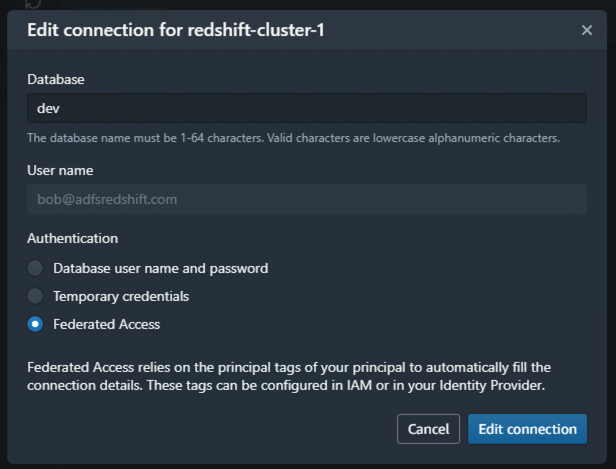
--conf spark.dynamicAllocation.enabled=false 
--conf spark.shuffle.service.enabled=false

Dynamic resource allocation is a different concept from automatic scaling in Amazon EKS, such as the Cluster Autoscaler. Disabling the dynamic allocation feature only fixes our 6-node Spark cluster size per job, but doesn’t stop the Amazon EKS cluster from expanding or shrinking automatically. It means our Amazon EKS cluster is still able to scale between 1 and 30 EC2 instances, as configured in the following code:

managedNodeGroups: 
  - name: mn-od
    availabilityZones: ["us-east-1b"] 
    instanceType: c5d.9xlarge
    minSize: 1
    desiredCapacity: 1
    maxSize: 30

Spark Adaptive Query Execution (AQE) is an optimization technique in Spark SQL since Spark 3.0. It dynamically re-optimizes the query execution plan at runtime, which supports a variety of optimizations, such as the following:

  • Dynamically switch join strategies
  • Dynamically coalesce shuffle partitions
  • Dynamically handle skew joins

The feature is enabled by default in EMR runtime for Spark, but disabled by default in open-source Apache Spark 3.1.2. To provide the fair comparison, make sure it’s set in the open-source Spark benchmark job declaration:

  sparkConf:
    # Enable AQE
    "spark.sql.adaptive.enabled": "true"
    "spark.sql.adaptive.localShuffleReader.enabled": "true"
    "spark.sql.adaptive.coalescePartitions.enabled": "true"
    "spark.sql.adaptive.skewJoin.enabled": "true"

Walkthrough overview

With these considerations in mind, we run three Spark jobs in Amazon EKS. This helps us compare Spark 3.1.2 performance in various deployment scenarios. For more details, check out the GitHub repository.

In this walkthrough, we show you how to do the following:

  • Produce a 3 TB TPC-DS complaint dataset
  • Run a benchmark job with the open-source Spark operator on Amazon EKS
  • Run the same benchmark application with Amazon EMR on EKS

We also provide information on how to benchmark with Amazon EMR on Amazon EC2.

Prerequisites

Install the following tools for the benchmark test:

Provision resources

The provision script creates the following resources:

  • A new Amazon EKS cluster
  • Amazon EMR on EKS enabler
  • The required AWS Identity and Access Management (IAM) roles
  • The S3 bucket emr-on-eks-nvme-${ACCOUNTID}-${AWS_REGION}, referred to as <S3BUCKET> in the following steps

The provisioning process takes approximately 30 minutes.

  1. Download the project with the following command:
    git clone https://github.com/aws-samples/emr-on-eks-bencharmk.git
    cd emr-on-eks-bencharmk

  2. Create a test environment (change the Region if necessary):
    export EKSCLUSTER_NAME=eks-nvme
    export AWS_REGION=us-east-1
    
    ./provision.sh

Modify the script if needed for testing against an existing Amazon EKS cluster. Make sure the existing cluster has the Cluster Autoscaler and Spark Operator installed. Examples are provided by the script.

  1. Validate the setup:
    # should return results
    kubectl get pod -n oss | grep spark-operator
    kubectl get pod -n kube-system | grep nodescaler

Generate TPC-DS test data (optional)

In this optional task, you generate TPC-DS test data in s3://<S3BUCKET>/BLOG_TPCDS-TEST-3T-partitioned. The process takes approximately 80 minutes.

The job generates TPC-DS compliant datasets with your preferred scale. In this case, it creates 3 TB of source data (approximately 924 GB compressed) in Parquet format. We have pre-populated the source dataset in the S3 bucket blogpost-sparkoneks-us-east-1 in Region us-east-1. You can skip the data generation job if you want to have a quick start.

Be aware of that cross-Region data transfer latency will impact your benchmark result. It’s recommended to generate the source data to your S3 bucket if your test Region is different from us-east-1.

  1. Start the job:
    kubectl apply -f examples/tpcds-data-generation.yaml

  2. Monitor the job progress:
    kubectl get pod -n oss
    kubectl logs tpcds-data-generation-3t-driver -n oss

  3. Cancel the job if needed:
    kubectl delete -f examples/tpcds-data-generation.yaml

The job runs in the namespace oss with a service account called oss in Amazon EKS, which grants a minimum permission to access the S3 bucket via an IAM role. Update the example .yaml file if you have a different setup in Amazon EKS.

Benchmark for open-source Spark on Amazon EKS

Wait until the data generation job is complete, then update the default input location parameter (s3://blogpost-sparkoneks-us-east-1/blog/BLOG_TPCDS-TEST-3T-partitioned) to your S3 bucket in the tpcds-benchmark.yaml file.. Other parameters in the application can also be adjusted. Check out the comments in the yaml file for details. This process takes approximately 130 minutes.

If the data generation job is skipped, run the following steps without waiting.

  1. Start the job:
    kubectl apply -f examples/tpcds-benchmark.yaml

  2. Monitor the job progress:
    kubectl get pod -n oss
    kubectl logs tpcds-benchmark-oss-driver -n oss

  3. Cancel the job if needed:
    kubectl delete -f examples/tpcds-benchmark.yaml

The benchmark application outputs a CSV file capturing runtime per Spark SQL query and a JSON file with query execution plan details. You can use the collected metrics and execution plans to compare and analyze performance between different Spark runtimes (open-source Apache Spark vs. EMR runtime for Spark).

Benchmark with Amazon EMR on EKS

Wait for the data generation job finish before starting the benchmark for Amazon EMR on EKS. Don’t forget to change the input location (s3://blogpost-sparkoneks-us-east-1/blog/BLOG_TPCDS-TEST-3T-partitioned) to your S3 bucket. The output location is s3://<S3BUCKET>/EMRONEKS_TPCDS-TEST-3T-RESULT. If you use the pre-populated TPC-DS dataset, start the Amazon EMR on EKS benchmark without waiting. This process takes approximately 40 minutes.

  1. Start the job (change the Region if necessary):
    export EMRCLUSTER_NAME=emr-on-eks-nvme
    export AWS_REGION=us-east-1
    
    ./examples/emr6.5-benchmark.sh

Amazon EKS offers multi-tenant isolation and optimized resource allocation features, so it’s safe to run two benchmark tests in parallel on a single Amazon EKS cluster.

  1. Monitor the job progress in real time:
    kubectl get pod -n emr
    #run the command then search "execution time" in the log to analyze individual query's performance
    kubectl logs YOUR_DRIVER_POD_NAME -n emr spark-kubernetes-driver

  2. Cancel the job (get the IDs from the cluster list on the Amazon EMR console):
    aws emr-containers cancel-job-run --virtual-cluster-id <YOUR_VIRTUAL_CLUSTER_ID> --id <YOUR_JOB_ID>

The following are additional useful commands:

#Check volume status
kubectl exec -it YOUR_DRIVER_POD_NAME -c spark-kubernetes-driver -n emr -- df -h

#Login to a running driver pod
kubectl exec -it YOUR_DRIVER_POD_NAME -c spark-kubernetes-driver -n emr – bash

#Monitor compute resource usage
watch "kubectl top node"

Benchmark for Amazon EMR on Amazon EC2

Optionally, you can use the same benchmark solution to test Amazon EMR on Amazon EC2. Download the benchmark utility application JAR file from a running Kubernetes container, then submit a job via the Amazon EMR console. More details are available in the GitHub repository.

Clean up

To avoid incurring future charges, delete the resources generated if you don’t need the solution anymore. Run the following cleanup script (change the Region if necessary):

cd emr-on-eks-bencharmk

export EKSCLUSTER_NAME=eks-nvme
export AWS_REGION=us-east-1

./deprovision.sh

Conclusion

Without making any application changes, we can run Apache Spark workloads faster and cheaper with Amazon EMR on EKS when compared to Apache Spark on Amazon EKS. We used a benchmark solution running on a 6-node c5d.9xlarge Amazon EKS cluster and queried a TPC-DS dataset at 3 TB scale. The performance test result shows that Amazon EMR on EKS provides up to 61% lower costs and up to 68% performance improvement over open-source Spark 3.1.2 on Amazon EKS.

If you’re wondering how much performance gain you can achieve with your use case, try out the benchmark solution or the EMR on EKS Workshop. You can also contact your AWS Solution Architects, who can be of assistance alongside your innovation journey.


About the Authors

Melody Yang is a Senior Big Data Solution Architect for Amazon EMR at AWS. She is an experienced analytics leader working with AWS customers to provide best practice guidance and technical advice in order to assist their success in data transformation. Her areas of interests are open-source frameworks and automation, data engineering and DataOps.

Kinnar Kumar Sen is a Sr. Solutions Architect at Amazon Web Services (AWS) focusing on Flexible Compute. As a part of the EC2 Flexible Compute team, he works with customers to guide them to the most elastic and efficient compute options that are suitable for their workload running on AWS. Kinnar has more than 15 years of industry experience working in research, consultancy, engineering, and architecture.

Modernize your healthcare clinical quality data repositories with Amazon Redshift Data Vault

Post Syndicated from Sarathi Balakrishnan original https://aws.amazon.com/blogs/big-data/modernize-your-healthcare-clinical-quality-data-repositories-with-amazon-redshift-data-vault/

With the shift to value-based care, tapping data to its fullest to improve patient satisfaction tops the priority of healthcare executives everywhere. To achieve this, reliance on key technology relevant to their sphere is a must. This is where data lakes can help. A data lake is an architecture that can assist providers in storing, sharing, and utilizing electronic health records and other patient data. Healthcare organizations are already utilizing data lakes to unite heterogeneous data from across hospital systems. The use of data lakes has aided in the effective transformation of the organizational culture, resulting in a data-driven approach to resolving issues. Healthcare clinical quality metric systems stream massive amounts of structured and semi-structured data into a data lake in real time from various sources. However, storing structured data in a data lake and applying schema-on-read leads to quality issues and adds complexity to the simple structured data process.

In this post, we demonstrate how to modernize your clinical quality data repositories with Amazon Redshift Data Vault.

How healthcare systems use data lakes

Data lakes are popular in healthcare systems because they allow the integration and exploratory analysis of diverse data. Data lakes comprise multiple data assets stored within a Hadoop ecosystem with minimal alterations to the original data format (or file). Because of this, the data lake lacks schema-on-write functionality. In data lakes, information is accessed using a methodology called schema-on-read. On the other hand, a data warehouse is a subject-oriented, time-variant, and centrally controlled database system designed for the management of mixed workloads and large queries. The schema of the data warehouse is predefined, the data written to it must conform to its schema (schema-on-write). It’s perfect for structured data storage.

Because the healthcare industry wants to preserve the data in raw format for compliance and regulatory requirements, data lakes are widely used in clinical quality tracking systems even though the incoming data are structured and semi-structured. For business and analytical use cases, the data in a data lake is further converted into a dimensional schema and loaded into a data warehouse. Data warehouses require several months of modeling, mapping, ETL (extract, transform, and load) planning and creation, and testing. The result is consistent, validated data for reporting and analytics.

The following diagram shows a typical clinical quality repository in a current healthcare system.

Data lakes offer information in its raw form, as well as a specialized means to obtaining data that applies the schema-on-read. In general, data lake users are experienced analysts familiar with data wrangling techniques that apply schema-on-read or understand data content from unstructured formats. Business users and data visualization builders struggle in the absence of powerful purpose-built search capabilities and data extraction algorithms. That isn’t to say data lakes are devoid of metadata or rules controlling their use, security, or administration. It’s the exact opposite. A successful data lake structures its data in such a way that it promotes better and more efficient access, and reuses data management methods or provides new tools that increase search and general knowledge of the data content.

Challenges in the data lake

However, data modeling shouldn’t be disregarded while employing the schema-on-read approach to handle data. A lack of meaningful data structure might lead to data quality problems, integration issues, performance issues, and deviations from organizational goals. Storing structured data in a data lake and then applying schema-on-read generates problems with data quality and complicates a basic structured data operation. You can also keep these structured datasets in data warehouses by skipping the data lake, but this increases the complexity of scaling, data transformation, and loading (ETL). But data warehouse ETL jobs apply a large number of business rules and heavily transform the data from its raw form to make the data fit one or more business purposes.

Dimensional representation data warehouses are located close to business applications but away from the source. This brings new challenges, like reverse tracking the data to its source to identify potential data errors and keep the original source for regulatory validation. In clinical quality reporting and regulatory reporting, accuracy is key. To provide high accuracy and data quality, developers often reverse track the data to its original source. This is very complex and sometimes not possible in a data warehouse model because the data loses its raw form. Compared to data warehouses, data lakes perform poorly in terms of dataset identification, processing, and catalog management. It’s complex to securely share data in a data lake between accounts. Cloud data lakes show improvement in this area, but some human intervention is still needed to make sure the data catalogs and security match healthcare requirements and standards.

Design and build a Data Vault model in Amazon Redshift

Amazon Redshift is a relational database system based on the PostgreSQL standard. It’s designed to efficiently run online analytical processing (OLAP) queries on petabyte-scale data. It also offers other query-handling efficiencies such as parallel processing, columnar database design, column data compression, a query optimizer, and compiled query code. A cluster is at the heart of every Amazon Redshift deployment. Each cluster consists of a leader node and one or more compute nodes, all of which are linked by high-speed networks.

Amazon Redshift RA3 instances with managed storage allow you to choose the number of nodes based on your performance requirements. The RA3 instance type can scale your data warehouse storage capacity automatically without manual intervention, and without needing to add additional compute resources. The number of nodes you choose is determined by the quantity of your data and the query processing performance you want.

The following diagram illustrates the Amazon Redshift RA3 instance architecture.

The interface to your business intelligence application is provided by a leader node. It provides conventional PostgreSQL JDBC/ODBC query and response interfaces. It acts as a traffic cop, routing requests from client applications to the proper compute nodes and managing the results that are delivered. It also distributes ingested data to computing nodes so that your databases may be built.

Amazon Redshift features like streaming, RA3’s near-limitless storage, Amazon Redshift ML, the SUPER data type, automatic table optimization, materialized views, and Amazon Redshift Spectrum open up the possibility of modernizing healthcare clinical quality data repositories and standardizing the data model for fast access and high accuracy. These features make RA3 instances the perfect candidate for your clinical quality repository. Additionally, the data sharing capability in Amazon Redshift keeps a single source for truth across the organization and removes the need for data silos. It’s tightly coupled with other AWS services, which allows you to take advantage of the AWS Cloud ecosystem and get the most out of your data with less effort.

Standardizing data modeling has two benefits: it allows you to reuse technical and organizational procedures (for example, ETL and project management), and you can readily merge data from diverse contexts without much complication. Because storage is separated from the computing, the Amazon Redshift RA3 instance retains the classic data lake feature of storing huge amounts of data. On the data side, to keep the data close to its raw form, a Data Vault model is the ideal solution to this problem.

Data Vault is a methodology to speed up the development of data warehouse initiatives and keep the data close to its sources. The Data Vault 2.0 data modeling standards are popular because they stress the business keys by hashing the keys across entities. This eliminates the need for strong relationships between entities and their linkages within the delivery of business processes. Data Vault makes it easy to integrate with versatile data sources for completely different use cases than it’s originally designed for, due to the following features:

  • Entities can stand alone and be built on patterns, each with a well-defined purpose.
  • Because the data represents the source system and delivers business value, data silos are eliminated.
  • You can load data in parallel with the least number of dependencies.
  • Historized data is kept at the coarsest level of granularity possible.
  • You can implement flexible business rules independently of data loading. This reduces the time taken to load the data by 25%.
  • You can add new data sources without affecting the current model.

The following diagram shows a simple clinical quality data repository with the Data Vault model with Amazon Redshift.

The following shows a simple clinical quality business Data Vault model using Amazon Redshift materialized views.

The Data Vault architecture is divided into four stages:

  • Staging – A copy of the most recent modifications to data from the source systems is created. This layer doesn’t save history, and you can perform numerous alterations to the staged data while populating, such as data type changes or scaling, character set conversion, and the inclusion of metadata columns to enable subsequent processing.
  • Raw vault – This stores a history of all data from numerous source systems. Except for putting the data into source system independent targets, no filters or business transformations happen here.
  • Business vault – This is an optional offering that is frequently developed. It includes business computations and denormalizations with the goal of enhancing the speed and ease of access inside the consumption layer, known as the information mart layer.
  • Data mart layer – This is where data is most typically accessible by users, such as reporting dashboards or extracts. You can build multiple marts from a single Data Vault integration layer, and the most frequent data modeling choice for these marts is Star/Kimball schemas.

The Amazon Redshift RA3 instance capabilities we discussed enable the development of highly performant and cost-effective Data Vault solutions. The staging and raw layers, for example, are populated in micro-batches by one Amazon Redshift cluster 24 hours a day. You can build the business Data Vault layer once a day and pause it to save costs when completed, and any number of consumer Amazon Redshift clusters can access the results.

The following diagram shows the complete architecture of the clinical quality Data Vault.

The architecture has the following components:

  • Batched raw data is loaded into the staging database raw schema.
  • The data quality validated structured data is delivered immediately to the staging database curated schema.
  • Data from devices, EHR systems, and vendor medical systems are also sent directly into the Amazon Redshift staging database.
  • The Data Vault 2.0 approach is used in the Amazon Redshift producer cluster to standardize data structure and assure data integrity.
  • Materialized views make a business Data Vault.
  • The Amazon Redshift SUPER data type allows you to store and query semi-structured data.
  • Amazon Redshift data share capabilities securely exchange the Data Vault tables and views between departments.
  • Support for streaming ingestion in Amazon Redshift eliminates the need to stage data in Amazon S3 before ingesting it into Amazon Redshift.
  • Amazon Redshift allows you to offload the historical data to Amazon S3. Healthcare clinical quality tracking systems usually offload data older than 6–7 years old for archival.
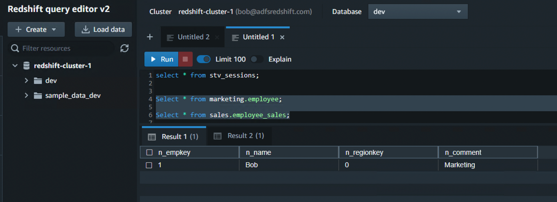
  • Amazon S3 and Amazon Redshift are HIPAA eligible.

Advantages of the Amazon Redshift clinical data repository

A clinical data repository in Amazon Redshift has the following benefits:

  • Data Vault enables the preservation of data as raw in its native form.
  • Amazon Redshift RA3 provides limitless storage, a real-time data feed, structured and semi-structured data, and more.
  • The new streaming functionality and analytics capacity in Amazon Redshift provide near-real-time analysis without the need for extra services.
  • Data quality is assured while maintaining data close to the business and source. You can reduce storage costs while maintaining data fidelity.
  • It’s compatible with business applications and allows for easy adoption when merging or expanding a variety of businesses without complexity.
  • The decoupled storage and compute option in Amazon Redshift allows for cost savings and offers ML capabilities within Amazon Redshift for quicker prediction, forecasting, and anomaly detection.

Conclusion

Data Vault is a one-of-a-kind database platform that promotes openness. It’s quick to adopt, infinitely configurable, and ready to overcome the most demanding data difficulties in current clinical quality metric tracking systems. Combined with the advantages of Amazon Redshift RA3 instances, Data Vault can outperform and deliver more value for cost and time.

To get started,

  • Create Amazon Redshift RA3 instance for the primary “Clinical Data Repository” and the data marts.
  • Build a Data vault schema for the raw vault an create materialized views for the business vault.
  • Enable Amazon Redshift data share to share data between producer cluster and consumer cluster.
  • Load the structed and unstructured data in to the producer cluster data vault for the business use.

About the Authors

Sarathi Balakrishnan is the Global Partner Solutions Architect, specializing in Data, Analytics and AI/ML at AWS. He works closely with AWS partner globally to build solutions and platforms on AWS to accelerate customers’ business outcomes with state-of-the-art cloud technologies and achieve more in their cloud explorations. He helps with solution architecture, technical guidance, and best practices to build cloud-native solutions. He joined AWS with over 20 years of large enterprise experience in agriculture, insurance, health care and life science, marketing and advertisement industries to develop and implement data and AI strategies.

Kasi Muthu is a Senior Partner Solutions Architect based in Houston, TX. He is a trusted advisor in Data, Analytics, AI/ML space. He also helps customers migrate their workloads to AWS with focus on scalability, resiliency, performance and sustainability. Outside of work, he enjoys spending time with his family and spending quite a bit of his free time on YouTube.

Email Routing Insights

Post Syndicated from Joao Sousa Botto original https://blog.cloudflare.com/email-routing-insights/

Email Routing Insights

Email Routing Insights

Have you ever wanted to try a new email service but worried it might lead to you missing any emails? If you have, you’re definitely not alone. Some of us email ourselves to make sure it reaches the correct destination, others don’t rely on a new address for anything serious until they’ve seen it work for a few days. In any case, emails often contain important information, and we need to trust that our emails won’t get lost for any reason.

To help reduce these worries about whether emails are being received and forwarded – and for troubleshooting if needed – we are rolling out a new Overview page to Email Routing. On the Overview tab people now have full visibility into our service and can see exactly how we are routing emails on their behalf.

Routing Status and Metrics

The first thing you will see in the new tab is an at a glance view of the service. This includes the routing status (to know if the service is configured and running), whether the necessary DNS records are configured correctly, and the number of custom and destination addresses on the zone.

Email Routing Insights

Below the configuration summary, you will see more advanced statistics about the number of messages received on your custom addresses, and what happened to those messages. You will see information about the number of emails forwarded or dropped by Email Routing (based on the rules you created), and the number that fall under other scenarios such as being rejected by Email Routing (due to errors, not passing security checks or being considered spam) or rejected by your destination mailbox. You now have the exact counts and a chart, so that you can track these metrics over time.

Email Routing Insights

Activity Log

On the Cloudflare Email Routing tab you’ll also see the Activity Log, where you can drill deeper into specific behaviors. These logs show you details about the email messages that reached one of the custom addresses you have configured on your Cloudflare zone.

For each message the logs will show you the Message ID, Sender, Custom Address, when Cloudflare Email Routing received it, and the action that was taken. You can also expand the row to see the SPF, DMARC, and DKIM status of that message along with any relevant error messaging.

And we know looking at every message can be overwhelming, especially when you might be resorting to the logs for troubleshooting purposes, so you have a few options for filtering:

  • Search for specific people (email addresses) that have messaged you.
  • Filter to show only one of your custom addresses.
  • Filter to show only messages where a specific action was taken.
Email Routing Insights

Routes and Settings

Next to the Overview tab, you will find the Routes tab with the configuration UI that is likely already familiar to you. That’s where you create custom addresses, add and verify destination addresses, and create rules with the relationships between the custom and destination addresses.

Email Routing Insights

Lastly the Settings tab includes less common actions such as the DNS configuration and the options for off boarding from Email Routing.

We hope you enjoy this update. And if you have any questions or feedback about this product, please come see us in the Cloudflare Community and the Cloudflare Discord.