Tag Archives: Analytics

Author AWS Glue jobs with PyCharm using AWS Glue interactive sessions

Post Syndicated from Kunal Ghosh original https://aws.amazon.com/blogs/big-data/author-aws-glue-jobs-with-pycharm-using-aws-glue-interactive-sessions/

Data lakes, business intelligence, operational analytics, and data warehousing share a common core characteristic—the ability to extract, transform, and load (ETL) data for analytics. Since its launch in 2017, AWS Glue has provided serverless data integration service that makes it easy to discover, prepare, and combine data for analytics, machine learning, and application development.

AWS Glue interactive sessions allows programmers to build, test, and run data preparation and analytics applications. Interactive sessions provide access to run fully managed serverless Apache Spark using an on-demand model. AWS Glue interactive sessions also provide advanced users the same Apache Spark engine as AWS Glue 2.0 or AWS Glue 3.0, with built-in cost controls and speed. Additionally, development teams immediately become productive using their existing development tool of choice.

In this post, we walk you through how to use AWS Glue interactive sessions with PyCharm to author AWS Glue jobs.

Solution overview

This post provides a step-by-step walkthrough that builds on the instructions in Getting started with AWS Glue interactive sessions. It guides you through the following steps:

  1. Create an AWS Identity and Access Management (IAM) policy with limited Amazon Simple Storage Service (Amazon S3) read privileges and associated role for AWS Glue.
  2. Configure access to a development environment. You can use a desktop computer or an OS running on the AWS Cloud using Amazon Elastic Compute Cloud (Amazon EC2).
  3. Integrate AWS Glue interactive sessions with an integrated development environments (IDE).

We use the script Validate_Glue_Interactive_Sessions.ipynb for validation, available as a Jupyter notebook.

Prerequisites

You need an AWS account before you proceed. If you don’t have one, refer to How do I create and activate a new AWS account? This guide assumes that you already have installed Python and PyCharm. Python 3.7 or later is the foundational prerequisite.

Create an IAM policy

The first step is to create an IAM policy that limits read access to the S3 bucket s3://awsglue-datasets, which has the AWS Glue public datasets. You use IAM to define the policies and roles for access to AWS Glue.

  1. On the IAM console, choose Policies in the navigation pane.
  2. Choose Create policy.
  3. On the JSON tab, enter the following code:
    {
        "Version": "2012-10-17",
        "Statement": [
            {
                "Effect": "Allow",
                "Action": [
                    "s3:Get*",
                    "s3:List*",
                    "s3-object-lambda:Get*",
                    "s3-object-lambda:List*"
                ],
                "Resource": ["arn:aws:s3:::awsglue-datasets/*"]
            }
        ]
    }

  4. Choose Next: Tags.
  5. Choose Next: Review.
  6. For Policy name, enter glue_interactive_policy_limit_s3.
  7. For Description, enter a description.
  8. Choose Create policy.

Create an IAM role for AWS Glue

To create a role for AWS Glue with limited Amazon S3 read privileges, complete the following steps:

  1. On the IAM console, choose Roles in the navigation pane.
  2. Choose Create role.
  3. For Trusted entity type, select AWS service.
  4. For Use cases for other AWS services, choose Glue.
  5. Choose Next.
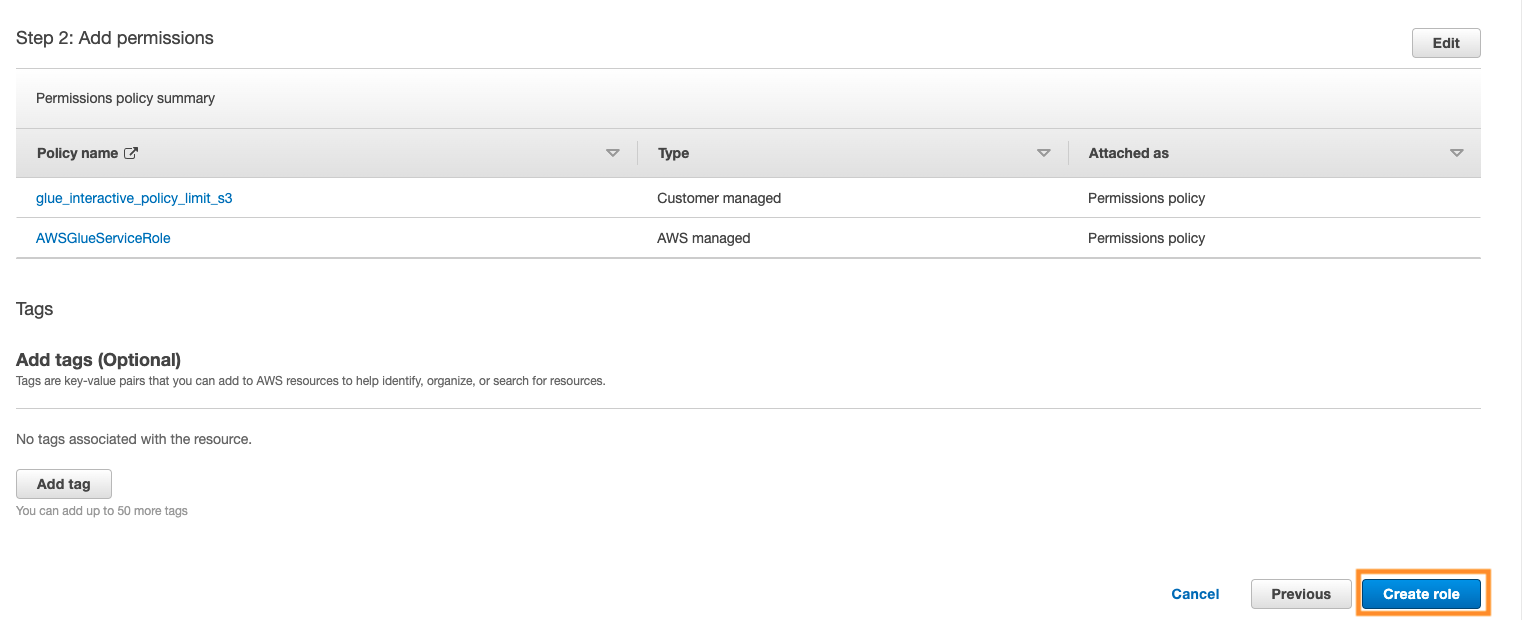
  6. On the Add permissions page, search and choose the AWS managed permission policies AWSGlueServiceRole and glue_interactive_policy_limit_s3.
  7. Choose Next.
  8. For Role name, enter glue_interactive_role.
  9. Choose Create role.
  10. Note the ARN of the role, arn:aws:iam::<replacewithaccountID>:role/glue_interactive_role.

Set up development environment access

This secondary level of access configuration needs to occur on the developer’s environment. The development environment can be a desktop computer running Windows or Mac/Linux, or similar operating systems running on the AWS Cloud using Amazon EC2. The following steps walk through each client access configuration. You can select the configuration path that is applicable to your environment.

Set up a desktop computer

To set up a desktop computer, we recommend completing the steps in Getting started with AWS Glue interactive sessions.

Set up an AWS Cloud-based computer with Amazon EC2

This configuration path follows the best practices for providing access to cloud-based resources using IAM roles. For more information, refer to Using an IAM role to grant permissions to applications running on Amazon EC2 instances.

  1. On the IAM console, choose Roles in the navigation pane.
  2. Choose Create role.
  3. For Trusted entity type¸ select AWS service.
  4. For Common use cases, select EC2.
  5. Choose Next.
  6. Add the AWSGlueServiceRole policy to the newly created role.
  7. On the Add permissions menu, choose Create inline policy.
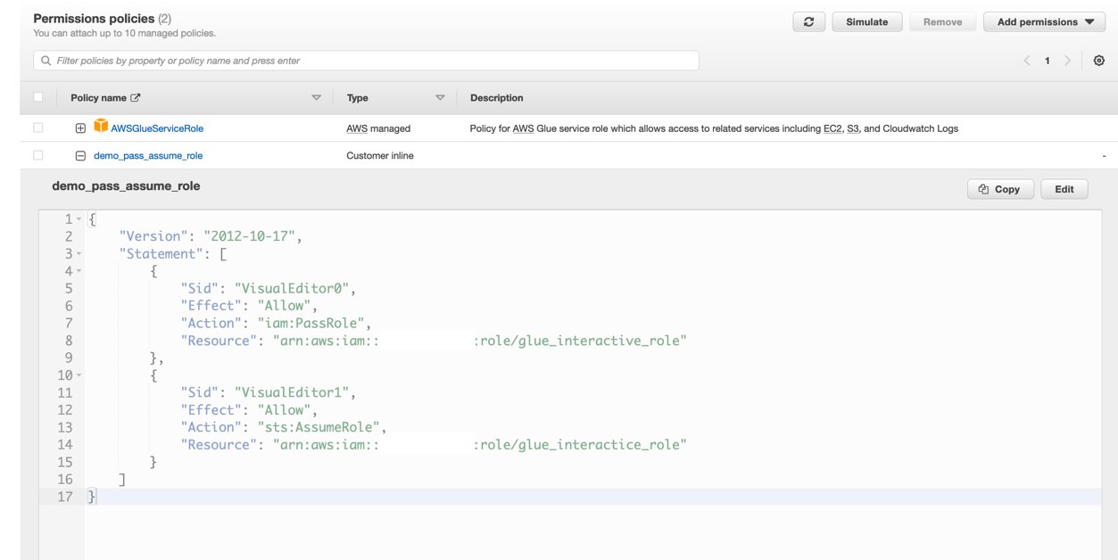
  8. Create an inline policy that allows the instance profile role to pass or assume glue_interactive_role and save the new role as ec2_glue_demo.

Your new policy is now listed under Permissions policies.

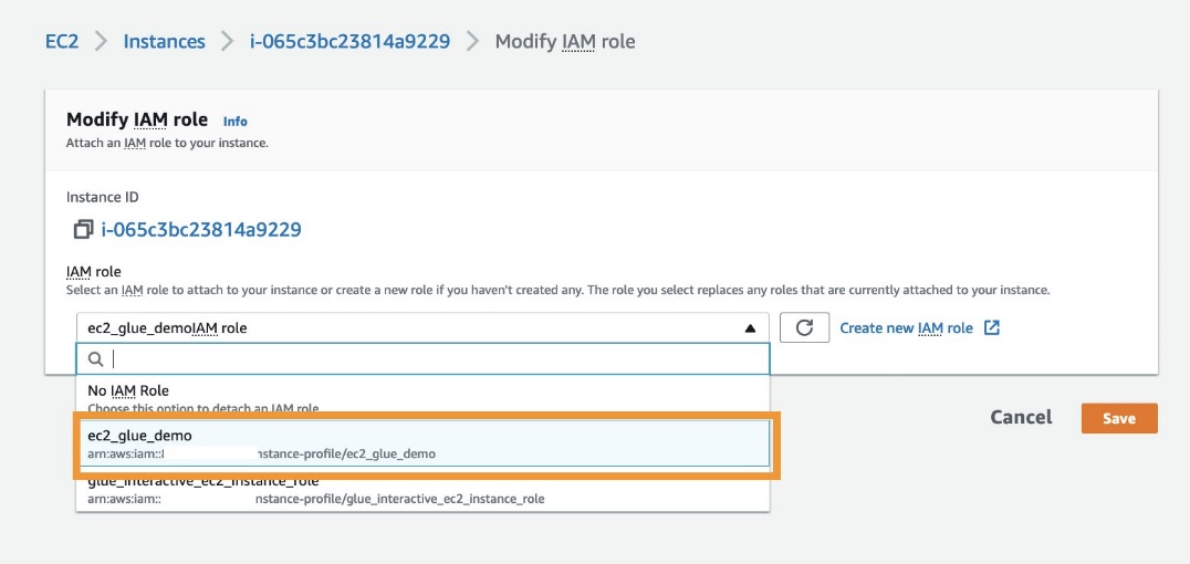
  1. On the Amazon EC2 console, choose (right-click) the instance you want to attach to the newly created role.
  2. Choose Security and choose Modify IAM role.
  3. For IAM role¸ choose the role ec2_glue_demo.
  4. Choose Save.
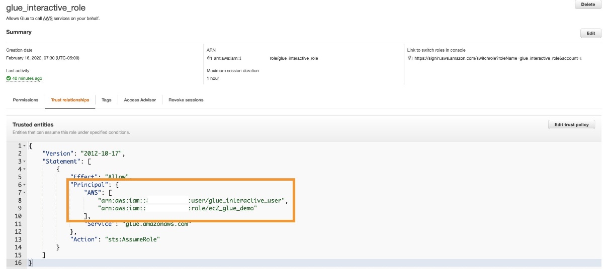
  5. On the IAM console, open and edit the trust relationship for glue_interactive_role.
  6. Add “AWS”: [“arn:aws:iam:::user/glue_interactive_user”,”arn:aws:iam:::role/ec2_glue_demo”] to the principal JSON key.
  7. Complete the steps detailed in Getting started with AWS Glue interactive sessions.

You don’t need to provide an AWS access key ID or AWS secret access key as part of the remaining steps.

Integrate AWS Glue interactive sessions with an IDE

You’re now ready to set up and validate your PyCharm integration with AWS Glue interactive sessions.

  1. On the welcome page, choose New Project.
  2. For Location, enter the location of your project glue-interactive-demo.
  3. Expand Python Interpreter.
  4. Select Previously configured interpreter and choose the virtual environment you created earlier.
  5. Choose Create.

The following screenshot shows the New Project page on a Mac computer. A Windows computer setup will have a relative path beginning with C:\ followed by the PyCharm project location.

  1. Choose the project (right-click) and on the New menu, choose Jupyter Notebook.
  2. Name the notebook Validate_Glue_Interactive_Sessions.

The notebook has a drop-down called Managed Jupyter server: auto-start, which means the Jupyter server automatically starts when any notebook cell is run.

  1. Run the following code:
    print("This notebook will start the local Python kernel")

You can observe that the Jupyter server started running the cell.

  1. On the Python 3 (ipykernal) drop-down, choose Glue PySpark.
  2. Run the following code to start a Spark session:
    spark

  3. Wait to receive the message that a session ID has been created.
  4. Run the following code in each cell, which is the boilerplate syntax for AWS Glue:
    import sys
    from awsglue.transforms import *
    from awsglue.utils import getResolvedOptions
    from pyspark.context import SparkContext
    from awsglue.context import GlueContext
    from awsglue.job import Job
    glueContext = GlueContext(SparkContext.getOrCreate())

  5. Read the publicly available Medicare Provider payment data in the AWS Glue data preparation sample document:
    medicare_dynamicframe = glueContext.create_dynamic_frame.from_options(
        's3',
        {'paths': ['s3://awsglue-datasets/examples/medicare/Medicare_Hospital_Provider.csv']},
        'csv',
        {'withHeader': True})
    print("Count:",medicare_dynamicframe.count())
    medicare_dynamicframe.printSchema()

  6. Change the data type of the provider ID to long to resolve all incoming data to long:
    medicare_res = medicare_dynamicframe.resolveChoice(specs = [('Provider Id','cast:long')])
    medicare_res.printSchema()

  7. Display the providers:
    medicare_res.toDF().select('Provider Name').show(10,truncate=False)

Clean up

You can run %delete_session which deletes the current session and stops the cluster, and the user stops being charged. Have a look at the AWS Glue interactive sessions magics. Also please remember to delete IAM policy and role once you are done.

Conclusion

In this post, we demonstrated how to configure PyCharm to integrate and work with AWS Glue interactive sessions. The post builds on the steps in Getting started with AWS Glue interactive sessions to enable AWS Glue interactive sessions to work with Jupyter notebooks. We also provided ways to validate and test the functionality of the configuration.


About the Authors

Kunal Ghosh is a Sr. Solutions Architect at AWS. His passion is building efficient and effective solutions on cloud, especially involving analytics, AI, data science, and machine learning. Besides family time, he likes reading and watching movies. He is a foodie.

Sebastian Muah is a Solutions Architect at AWS focused on analytics, AI/ML, and big data. He has over 25 years of experience in information technology and helps customers architect and build highly scalable, performant, and secure cloud-based solutions on AWS. He enjoys cycling and building things around his home.

Query 10 new data sources with Amazon Athena

Post Syndicated from Scott Rigney original https://aws.amazon.com/blogs/big-data/query-10-new-data-sources-with-amazon-athena/

When we first launched Amazon Athena, our mission was to make it simple to query data stored in Amazon Simple Storage Service (Amazon S3). Athena customers found it easy to get started and develop analytics on petabyte-scale data lakes, but told us they needed to join their Amazon S3 data with data stored elsewhere. We added connectors to sources including Amazon DynamoDB and Amazon Redshift to give data analysts, data engineers, and data scientists the ability to run SQL queries on data stored in databases running on-premises or in the cloud alongside data stored in Amazon S3.

Today, thousands of AWS customers from nearly every industry use Athena federated queries to surface insights and make data-driven decisions from siloed enterprise data—using a single AWS service and SQL dialect.

We’re excited to expand your ability to derive insights from more of your data with today’s release of 10 new data source connectors, which include some of the most widely used data stores on the market.

New data sources for Athena

You can now use Athena to query and surface insights from 10 new data sources:

  • SAP HANA (Express Edition)
  • Teradata
  • Cloudera
  • Hortonworks
  • Snowflake
  • Microsoft SQL Server
  • Oracle
  • Azure Data Lake Storage (ADLS) Gen2
  • Azure Synapse
  • Google BigQuery

Today’s release greatly expands the number of data sources supported by Athena. For a complete list of supported data sources, see Using Athena Data Source Connectors.

To coincide with this release, we enhanced the Athena console to help you browse available sources and connect to your data in fewer steps. You can now search, sort, and filter the available connectors on the console, and then follow the guided setup wizard to connect to your data.

Just as before, we’ve open-sourced the new connectors to invite contributions from the developer community. For more information, see Writing a Data Source Connector Using the Athena Query Federation SDK.

Connect the dots in your analytics strategy with Athena

With the breadth of data storage options available today, it’s common for data-driven organizations to choose a data store that meets the requirements of specific use cases and applications. Although this flexibility is ideal for architects and developers, it can add complexity for analysts, data scientists, and data engineers, which prevents them from accessing the data they need. To get around this, many users resort to workarounds that often involve learning new programming languages and database concepts or building data pipelines to prepare the data before it can be analyzed. Athena helps cut through this complexity with support for over 25 data sources and its simple-to-use, pay-as-you-go, serverless design.

With Athena, you can use your existing SQL knowledge to extract insights from a wide range of data sources without learning a new language, developing scripts to extract (and duplicate) data, or managing infrastructure. Athena allows you to do the following:

  • Run on-demand analysis on data spread across multiple cloud providers and systems of record using a single tool and single SQL dialect
  • Visualize data in business intelligence applications that use Athena to perform complex, multi-source joins
  • Design self-service extract, transform, and load (ETL) pipelines and event-based data processing workflows with Athena’s integration with AWS Step Functions
  • Unify diverse data sources to produce rich input features for machine learning model training workflows
  • Develop user-facing data-as-a-product applications that surface insights across data mesh architectures
  • Support analytics use cases while your organization migrates on-premises sources to the AWS Cloud

Get started with Athena’s data source connectors

To get started with federated queries for Athena, on the Athena console, choose Data Sources in the navigation pane, choose a data source, and follow the guided setup experience to configure your connector. After the connection is established and the source is registered with Athena, you can query the data via the Athena console, API, AWS SDK, and compatible third-party applications. To learn more, see Using Amazon Athena Federated Query and Writing Federated Queries.

You can also share a data source connection with team members, allowing them to use their own AWS account to query the data without setting up a duplicate connector. To learn more, see Enabling Cross-Account Federated Queries.

Conclusion

We encourage you to evaluate Athena and federated queries on your next analytics project. For help getting started, we recommend the following resources:


About the Authors

Scott Rigney is a Senior Technical Product Manager with Amazon Web Services (AWS) and works with the Amazon Athena team based out of Arlington, Virginia. He is passionate about building analytics products that enable enterprises to make data-driven decisions.

Jean-Louis Castro-Malaspina is a Senior Product Marketing Manager with Amazon Web Services (AWS) based in Hershey, Pennsylvania. He enjoys highlighting how customers use Analytics and Amazon Athena to unlock innovation. Outside of work, Jean-Louis enjoys spending time with his wife and daughter, running, and following international soccer.

Suresh_90Suresh Akena is a Principal WW GTM Leader for Amazon Athena. He works with the startups, enterprise and strategic customers to provide leadership on large scale data strategies including migration to AWS platform, big data and analytics and ML initiatives and help them to optimize and improve time to market for data driven applications when using AWS.

Build your data pipeline in your AWS modern data platform using AWS Lake Formation, AWS Glue, and dbt Core

Post Syndicated from Benjamin Menuet original https://aws.amazon.com/blogs/big-data/build-your-data-pipeline-in-your-aws-modern-data-platform-using-aws-lake-formation-aws-glue-and-dbt-core/

dbt has established itself as one of the most popular tools in the modern data stack, and is aiming to bring analytics engineering to everyone. The dbt tool makes it easy to develop and implement complex data processing pipelines, with mostly SQL, and it provides developers with a simple interface to create, test, document, evolve, and deploy their workflows. For more information, see docs.getdbt.com.

dbt primarily targets cloud data warehouses such as Amazon Redshift or Snowflake. Now, you can use dbt against AWS data lakes, thanks to the following two services:

In this post, you’ll learn how to deploy a data pipeline in your modern data platform using the dbt-glue adapter built by the AWS Professional Services team in collaboration with dbtlabs.

With this new open-source, battle-tested dbt AWS Glue adapter, developers can now use dbt for their data lakes, paying for just the compute they need, with no need to shuffle data around. They still have access to everything that makes dbt great, including the local developer experience, documentation, tests, incremental data processing, Git integration, CI/CD, and more.

Solution overview

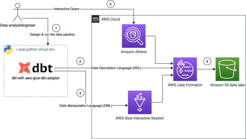
The following diagram shows the architecture of the solution.

The steps in this workflow are as follows:

  1. The data team configures a local Python virtual environment and creates a data pipeline with dbt.
  2. The dbt-glue adapter uses Lake Formation to perform all structure manipulation, like creation of database, tables. or views.
  3. The dbt-glue adapter uses AWS Glue interactive sessions as the backend for processing your data.
  4. All data is stored in Amazon Simple Storage Service (Amazon S3) as Parquet open file format.
  5. The data team can now query all data stored in the data lake using Amazon Athena.

Walkthrough overview

For this post, you run a data pipeline that creates indicators based on NYC taxi data by following these steps:

  1. Deploy the provided AWS CloudFormation stack in Region us-east-1.
  2. Configure your Amazon CloudShell environment.
  3. Install dbt, the dbt CLI, and the dbt adaptor.
  4. Use CloudShell to clone the project and configure it to use your account’s configuration.
  5. Run dbt to implement the data pipeline.
  6. Query the data with Athena.

For our use case, we use the data from the New York City Taxi Records dataset. This dataset is available in the Registry of Open Data on AWS (RODA), which is a repository containing public datasets from AWS resources.

The CloudFormation template creates the nyctaxi database in your AWS Glue Data Catalog and a table (records) that points to the public dataset. You don’t need to host the data in your account.

Prerequisites

The CloudFormation template used by this project configures the AWS Identity and Access Management (IAM) role GlueInteractiveSessionRole with all the mandatory permissions.

For more details on permissions for AWS Glue interactive sessions, refer to Securing AWS Glue interactive sessions with IAM.

Deploy resources with AWS CloudFormation

The CloudFormation stack deploys all the required infrastructure:

  • An IAM role with all the mandatory permissions to run an AWS Glue interactive session and the dbt-glue adapter.
  • An AWS Glue database and table to store the metadata related to the NYC taxi records dataset
  • An S3 bucket to use as output and store the processed data
  • An Athena configuration (a workgroup and S3 bucket to store the output) to explore the dataset
  • An AWS Lambda function as an AWS CloudFormation custom resource that updates all the partitions in the AWS Glue table

To create these resources, choose Launch Stack and follow the instructions:

Configure the CloudShell environment

To start working with the shell, complete the following steps:

  1. Sign in to the AWS Management Console and launch CloudShell using either one of the following two methods:
    1. Choose the CloudShell icon on the console navigation bar.
    2. Enter cloudshell in the Find Services box and then choose the CloudShell option.
  2. Because dbt and the dbt-glue adapter are compatible with Python versions 3.7, 3.8, and 3.9, check the version of Python:
    $ python3 --version

  3. Configure a Python virtual environment to isolate the package version and code dependencies:
    $ sudo yum install git -y
    $ python3 -m venv dbt_venv
    $ source dbt_venv/bin/activate
    $ python3 -m pip install --upgrade pip

  4. Configure the aws-glue-session package:
    $ sudo yum install gcc krb5-devel.x86_64 python3-devel.x86_64 -y
    $ pip3 install --no-cache-dir --upgrade boto3
    $ pip3 install --no-cache-dir --upgrade aws-glue-sessions

Install dbt, the dbt CLI, and the dbt adaptor

The dbt CLI is a command-line interface for running dbt projects. It’s is free to use and available as an open source project. Install dbt and the dbt CLI with the following code:

$ pip3 install --no-cache-dir dbt-core

For more information, refer to How to install dbt, What is dbt?, and Viewpoint.

Install the dbt adapter with the following code:

$ pip3 install --no-cache-dir dbt-glue

Clone the project

The dbt AWS Glue interactive session demo project contains an example of a data pipeline that produces metrics based on NYC taxi dataset. Clone the project with the following code:

$ git clone https://github.com/aws-samples/dbtgluenyctaxidemo

This project comes with the following configuration example:

$ dbtgluenyctaxidemo/profile/profiles.yml

The following table summarizes the parameter options for the adaptor.

Option Description Mandatory
project_name The dbt project name. This must be the same as the one configured in the dbt project. yes
type The driver to use. yes
query-comment A string to inject as a comment in each query that dbt runs. no
role_arn The ARN of the interactive session role created as part of the CloudFormation template. yes
region The AWS Region were you run the data pipeline. yes
workers The number of workers of a defined workerType that are allocated when a job runs. yes
worker_type The type of predefined worker that is allocated when a job runs. Accepts a value of Standard, G.1X, or G.2X. yes
schema The schema used to organize data stored in Amazon S3. yes
database The database in Lake Formation. The database stores metadata tables in the Data Catalog. yes
session_provisioning_timeout_in_seconds The timeout in seconds for AWS Glue interactive session provisioning. yes
location The Amazon S3 location of your target data. yes
idle_timeout The AWS Glue session idle timeout in minutes. (The session stops after being idle for the specified amount of time.) no
glue_version The version of AWS Glue for this session to use. Currently, the only valid options are 2.0 and 3.0. The default value is 2.0. no
security_configuration The security configuration to use with this session. no
connections A comma-separated list of connections to use in the session. no

Run the dbt project

The objective of this sample project is to create the following four tables, which contain metrics based on the NYC taxi dataset:

  • silver_nyctaxi_avg_metrics – Basic metrics based on NYC Taxi Open Data for the year 2016
  • gold_nyctaxi_passengers_metrics – Metrics per passenger based on the silver metrics table
  • gold_nyctaxi_distance_metrics – Metrics per distance based on the silver metrics table
  • gold_nyctaxi_cost_metrics – Metrics per cost based on the silver metrics table
  1. To run the project dbt, you should be in the project folder:
    $ cd dbtgluenyctaxidemo

  2. The project requires you to set environment variables in order to run on the AWS account:
    $ export DBT_ROLE_ARN="arn:aws:iam::$(aws sts get-caller-identity --query "Account" --output text):role/GlueInteractiveSessionRole"
    $ export DBT_S3_LOCATION="s3://aws-dbt-glue-datalake-$(aws sts get-caller-identity --query "Account" --output text)-us-east-1/"

  3. Make sure the profile is set up correctly from the command line:
    $ dbt debug --profiles-dir profile

  4. Run the models with the following code:
    $ dbt run --profiles-dir profile

  5. Generate documentation for the project:
    $ dbt docs generate --profiles-dir profile

  6. View the documentation for the project:
    $ dbt docs serve --profiles-dir profile

Query data via Athena

This section demonstrates how to query the target table using Athena. To query the data, complete the following steps:

  1. On the Athena console, switch the workgroup to athena-dbt-glue-aws-blog.
  2. If the Workgroup athena-dbt-glue-aws-blog settings dialog box appears, choose Acknowledge.
  3. Use the following query to explore the metrics created by the dbt project:
    SELECT cm.avg_cost_per_minute
    , cm.avg_cost_per_distance
    , dm.avg_distance_per_duration
    , dm.year
    , dm.month
    , dm.type
    FROM "dbt_nyc_metrics"."gold_nyctaxi_distance_metrics" dm
    LEFT JOIN "dbt_nyc_metrics"."gold_nyctaxi_cost_metrics" cm
    ON dm.type = cm.type
    AND dm.year = cm.year
    AND dm.month = cm.month
    WHERE dm.type = 'yellow'
    AND dm.year = '2016'
    AND dm.month = '6'

The following screenshot shows the results of this query.

Clean Up

To clean up your environment, complete the following steps in CloudShell:

  1. Delete the database created by dbt:
    $ aws glue delete-database --name dbt_nyc_metrics

  2. Delete all generated data:
    $ aws s3 rm s3://aws-dbt-glue-datalake-$(aws sts get-caller-identity --query "Account" --output text)-us-east-1/ --recursive
    $ aws s3 rm 3://aws-athena-dbt-glue-query-results-$(aws sts get-caller-identity --query "Account" --output text)-us-east-1/ --recursive

  3. Delete the CloudFormation stack:
    $ aws cloudformation delete-stack --stack-name dbt-demo

Summary

This post demonstrates how AWS managed services are key enablers and accelerators to build a modern data platform at scale or take advantage of an existing one.

With the introduction of dbt and aws-glue-dbt-adapter, data teams can access data stored in your modern data platform using SQL statements to extract value from data.

To report a bug or request a feature, please open an issue on GitHub. If you have any questions or suggestions, leave your feedback in the comment section. If you need further assistance to optimize your modern data platform, contact your AWS account team or a trusted AWS Partner.


About the Authors

Benjamin Menuet is a Data Architect with AWS Professional Services. He helps customers develop big data and analytics solutions to accelerate their business outcomes. Outside of work, Benjamin is a trail runner and has finished some mythic races like the UTMB.

Armando Segnini is a Data Architect with AWS Professional Services. He spends his time building scalable big data and analytics solutions for AWS Enterprise and Strategic customers. Armando also loves to travel with his family all around the world and take pictures of the places he visits.

Moshir Mikael is a Senior Practice Manager with AWS Professional Services.  He led development of large enterprise data platforms in EMEA and currently leading the Professional Services teams in EMEA for analytics.

Anouar Zaaber is a Senior Engagement Manager in AWS Professional Services. He leads internal AWS teams, external partners, and customer teams to deliver AWS cloud services that enable customers to realize their business outcomes.

Amazon QuickSight 1-click public embedding available in preview

Post Syndicated from Kareem Syed-Mohammed original https://aws.amazon.com/blogs/big-data/amazon-quicksight-1-click-public-embedding-available-in-preview/

Amazon QuickSight is a fully managed, cloud-native business intelligence (BI) service that makes it easy to connect to your data, create interactive dashboards, and share these with tens of thousands of users, either directly within a QuickSight application, or embedded in web apps and portals.

QuickSight Enterprise Edition now supports 1-click public embedding, a feature that allows you to embed your dashboards into public applications, wikis, and portals without any coding or development needed. Anyone on the internet can start accessing these embedded dashboards with up-to-date information instantly, without any server deployments or infrastructure licensing needed! 1-click public embedding allows you to empower your end-users with access to insights.

In this post, we walk you through the steps to use this feature, demonstrate the end-user experience, and share sample use cases.

Solution overview

1-click public embedding requires an administrator of the QuickSight account to enable this feature and use session-based pricing. After you complete the prerequisites (see the following section), the 1-click embedding process involves three simple steps:

  1. Enable public access on the dashboard
  2. Allow list the domain where you want to embed the dashboard in QuickSight
  3. Embed the dashboard

Prerequisites

  1. The account needs to have session capacity pricing enabled
  2. As a prerequisite, make sure your QuickSight account is enabled for dashboards to be shared by the public. Because this feature allows dashboards to be enabled for any user, the usability of this feature must be enabled by an administrator of your QuickSight account with the following AWS Identity and Administration (IAM) permissions:
    {
        "Version": "2012-10-17",
        "Statement": [
            {
                "Action": "quicksight:UpdatePublicSharingSettings",
                "Resource": "*",
                "Effect": "Allow"
            }
         ]
    }

After you enable this policy, you can activate the account-level settings.

  1. Sign in to your QuickSight account.
  2. On the user name drop-down menu, choose Manage QuickSight.
  3. Choose Security & permissions in the navigation pane.
  4. Under Public access to dashboards, choose Manage.
  5. Enable the setting Everyone on the internet to allow public access.
  6. Confirm this setting and choose Accept.

Enabling this setting doesn’t automatically enable all the dashboards to be accessed by anyone on the internet. It gives the ability for authors of the dashboards to individually enable the dashboard to be accessed by anyone on the internet via the share link or when embedded.

Enable public access permissions on the dashboard

After you create a QuickSight dashboard, to enable public access, complete the following steps:

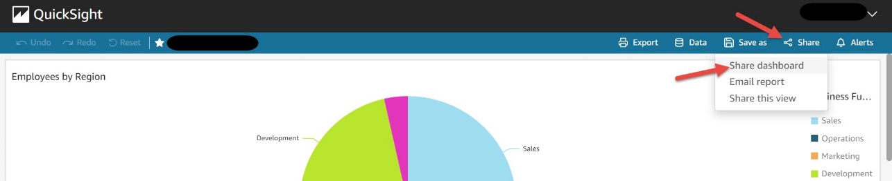
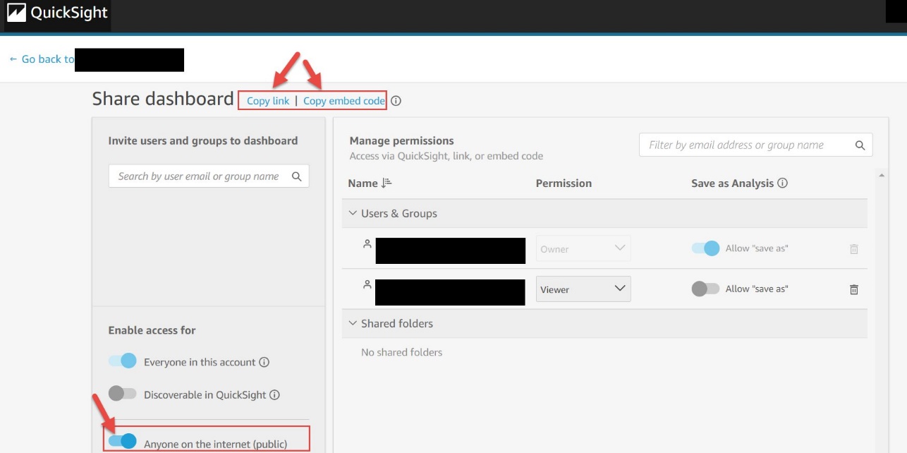
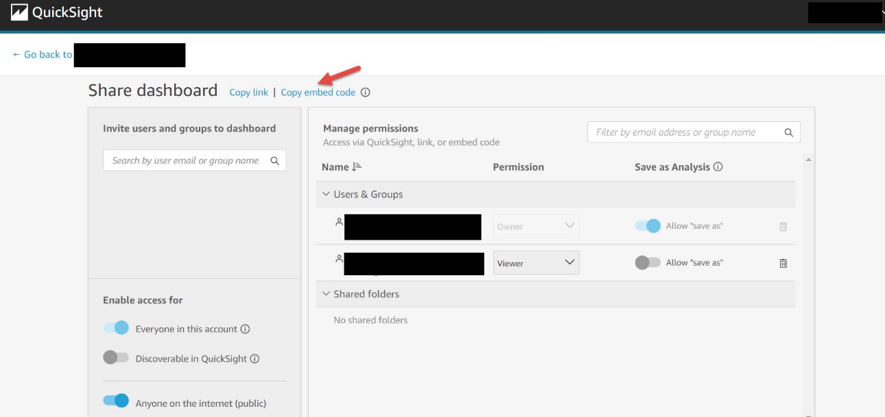
  1. On the QuickSight dashboard, on the Share menu, choose Share dashboard.

Only owners and co-owners of the dashboard can perform this action.

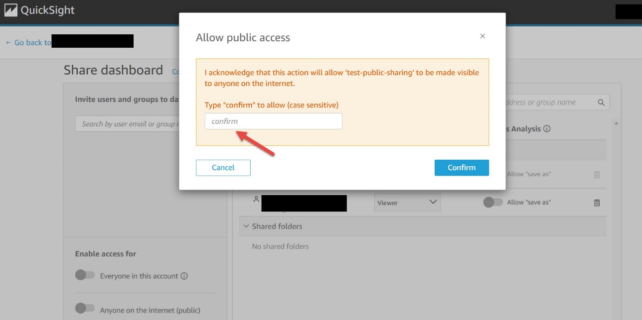
  1. Under Enable access for, turn on Anyone on the internet (public).

This setting allows you to share this dashboard with anyone on the internet via the share link or when embedded.

  1. Accept this setting and choose Confirm.

You now have the option to copy the link or the embed code to share the dashboard. Note that when this setting is enabled, the dashboard can only be accessed using the link or when embedded using the embed code.

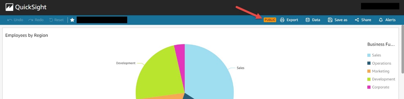
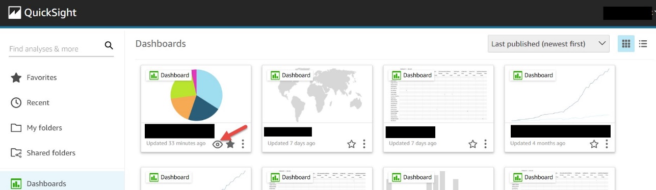
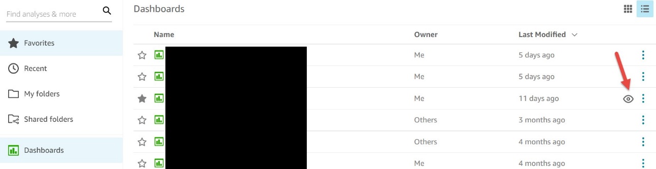
After you enable the dashboard for public access, you can see badges on the dashboard as follows.

The dashboard toolbar has a PUBLIC badge.

The dashboards grid view has an eye icon for each dashboard.

The dashboards list view has an eye icon for each dashboard.

Disable the public access

You can disable the public access of your dashboards in two ways:

  1. Disable the Anyone on the internet setting for the dashboard (to be done by the owners and co-owners of the dashboard).
  2. Disable the Public access to dashboard setting at the account level (to be done by the IAM admin). You can disable the account-level settings even if the dashboard-level setting is enabled. This still prevents the dashboards from being accessed publicly.

Allow list the domain where you want to embed the dashboard in QuickSight

The domain where the dashboard is to be embedded must be allow listed in QuickSight. For instructions, see Adding domains for embedded users.

Embed the dashboard

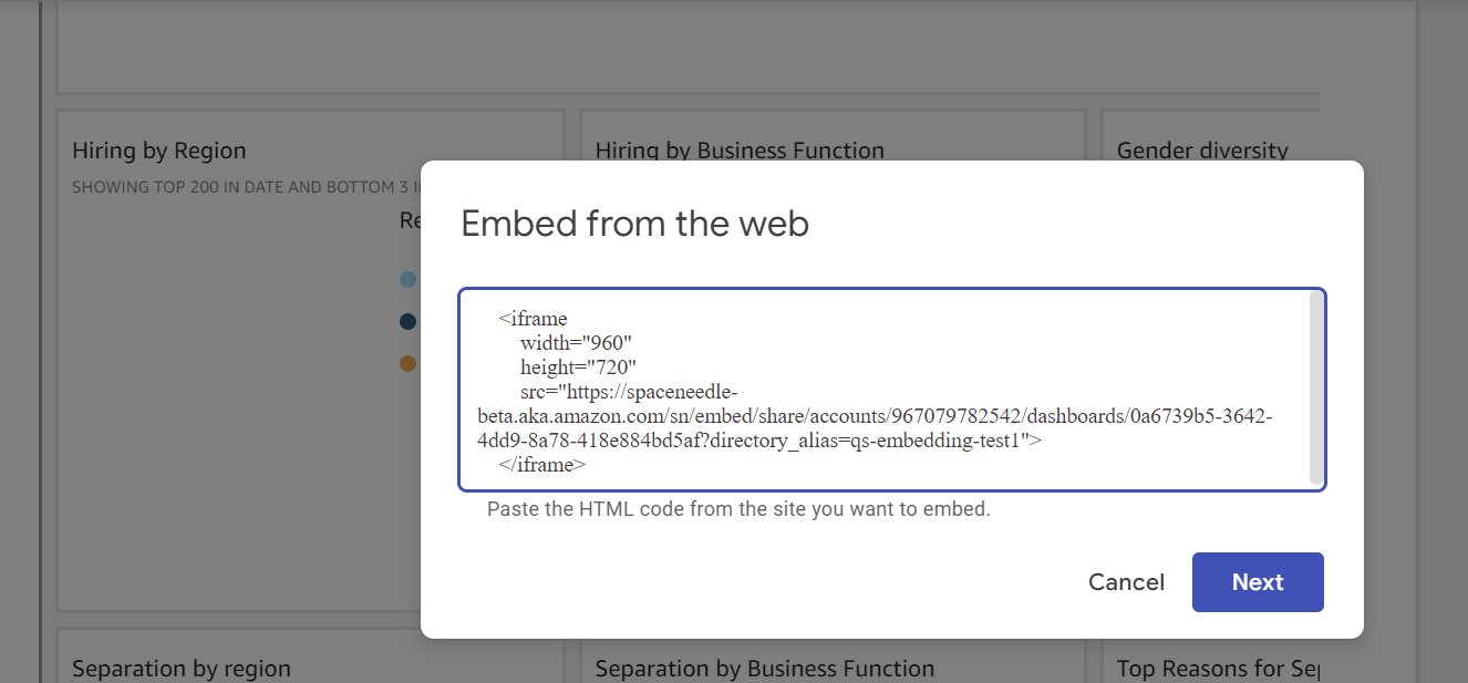
After you set your desired access to the dashboard, you can choose Copy embed code, which copies the embed code for that dashboard. This code embeds the dashboard when added to an internal application.

The copied embed code is similar to the following code:

    <iframe
        width="960"
        height="720"
        src="https://quicksight.aws.amazon.com/sn/
        embed/share/accounts/accountid/dashboards/dashboardid">
    </iframe>

To embed the dashboard in an HTML page, open the HTML of the page where you want to embed the dashboard and enter the copied embed code into the HTML code.

If your public-facing applications are built on Google Sites, to embed your dashboard, open the page on Google Sites, then choose Insert and Embed. A pop-up window appears with a prompt to enter a URL or embed code. Choose Embed code and enter the copied embed code in the text box.

Make sure to allow list the following domains in QuickSight when embedding in Google Sites: https://googleusercontent.com (enable subdomains), https://www.gstatic.com, and https://sites.google.com.

After you embed the dashboard in your application, anyone who can access your application can now access the embedded dashboard.

Sample use cases

1-click public embedding enables you to embed your dashboards into public applications, wikis, and portals without any coding or development needed. In this section, we present two sample use cases.

For our first use case, a fictitious school district uses 1-click public embedding to report on the teachers’ enrollment in the district. They built a dashboard and used this feature to embed it on their public-facing site.

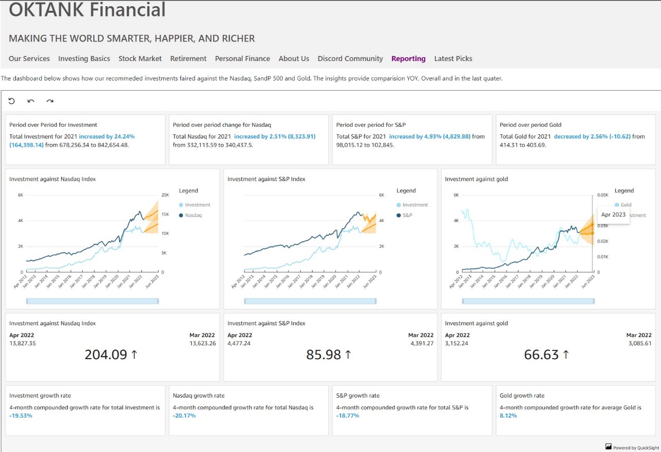
For our second use case, a fictitious fintech that provides investment solutions is using 1-click public embedding to show how their investment compares against other well-known indexes and commodities. They used this feature to add this comparison dashboard on their public-facing marketing pages.

Try out 1-click public embedding

To try out this feature, see Embed Amazon QuickSight dashboard in seconds. In this demo, you can change the dashboard between a logistics or sales dashboard by choosing Change Dashboard and entering the embed code for the dashboard you want to render on the site.

Conclusion

With 1-click public embedding, you can now embed rich and interactive QuickSight dashboards quickly and easily. Enable your end-users to dive deeper into their data through embedded dashboard with the click of a button—and with no infrastructure setup or management, scale to millions of users. 1-click public embedding is now in preview; to access this feature, please contact [email protected].

QuickSight also supports embedding in SaaS apps without any user management needed. For more information, refer to Embed multi-tenant dashboards in SaaS apps using Amazon QuickSight without provisioning or managing users.

To stay up to date on QuickSight embedded analytics, check out what’s new with the QuickSight User Guide.


About the Authors

Kareem Syed-Mohammed is a Product Manager at Amazon QuickSight. He focuses on embedded analytics, APIs, and developer experience. Prior to QuickSight he has been with AWS Marketplace and Amazon retail as a PM. Kareem started his career as a developer and then PM for call center technologies, Local Expert and Ads for Expedia. He worked as a consultant with McKinsey and Company for a short while.

Srikanth Baheti is a Specialized World Wide Sr. Solution Architect for Amazon QuickSight. He started his career as a consultant and worked for multiple private and government organizations. Later he worked for PerkinElmer Health and Sciences & eResearch Technology Inc, where he was responsible for designing and developing high traffic web applications, highly scalable and maintainable data pipelines for reporting platforms using AWS services and Serverless computing.-

Introducing AWS Glue Auto Scaling: Automatically resize serverless computing resources for lower cost with optimized Apache Spark

Post Syndicated from Noritaka Sekiyama original https://aws.amazon.com/blogs/big-data/introducing-aws-glue-auto-scaling-automatically-resize-serverless-computing-resources-for-lower-cost-with-optimized-apache-spark/

Data created in the cloud is growing fast in recent days, so scalability is a key factor in distributed data processing. Many customers benefit from the scalability of the AWS Glue serverless Spark runtime. Today, we’re pleased to announce the release of AWS Glue Auto Scaling, which helps you scale your AWS Glue Spark jobs automatically based on the requirements calculated dynamically during the job run, and accelerate job runs at lower cost without detailed capacity planning.

Before AWS Glue Auto Scaling, you had to predict workload patterns in advance. For example, in cases when you don’t have expertise in Apache Spark, when it’s the first time you’re processing the target data, or when the volume or variety of the data is significantly changing, it’s not so easy to predict the workload and plan the capacity for your AWS Glue jobs. Under-provisioning is error-prone and can lead to either missed SLA or unpredictable performance. On the other hand, over-provisioning can cause underutilization of resources and cost overruns. Therefore, it was a common best practice to experiment with your data, monitor the metrics, and adjust the number of AWS Glue workers before you deployed your Spark applications to production.

With AWS Glue Auto Scaling, you no longer need to plan AWS Glue Spark cluster capacity in advance. You can just set the maximum number of workers and run your jobs. AWS Glue monitors the Spark application execution, and allocates more worker nodes to the cluster in near-real time after Spark requests more executors based on your workload requirements. When there are idle executors that don’t have intermediate shuffle data, AWS Glue Auto Scaling removes the executors to save the cost.

AWS Glue Auto Scaling is available with the optimized Spark runtime on AWS Glue version 3.0, and you can start using it today. This post describes possible use cases and how it works.

Use cases and benefits for AWS Glue Auto Scaling

Traditionally, AWS Glue launches a serverless Spark cluster of a fixed size. The computing resources are held for the whole job run until it is completed. With the new AWS Glue Auto Scaling feature, after you enable it for your AWS Glue Spark jobs, AWS Glue dynamically allocates compute resource considering the given maximum number of workers. It also supports dynamic scale-out and scale-in of the AWS Glue Spark cluster size over the course of job. As more executors are requested by Spark, more AWS Glue workers are added to the cluster. When the executor has been idle without active computation tasks for a period of time and associated shuffle dependencies, the executor and corresponding worker are removed.

AWS Glue Auto Scaling makes it easy to run your data processing in the following typical use cases:

  • Batch jobs to process unpredictable amounts of data
  • Jobs containing driver-heavy workloads (for example, processing many small files)
  • Jobs containing multiple stages with uneven compute demands or due to data skews (for example, reading from a data store, repartitioning it to have more parallelism, and then processing further analytic workloads)
  • Jobs to write large amouns of data into data warehouses such as Amazon Redshift or read and write from databases

Configure AWS Glue Auto Scaling

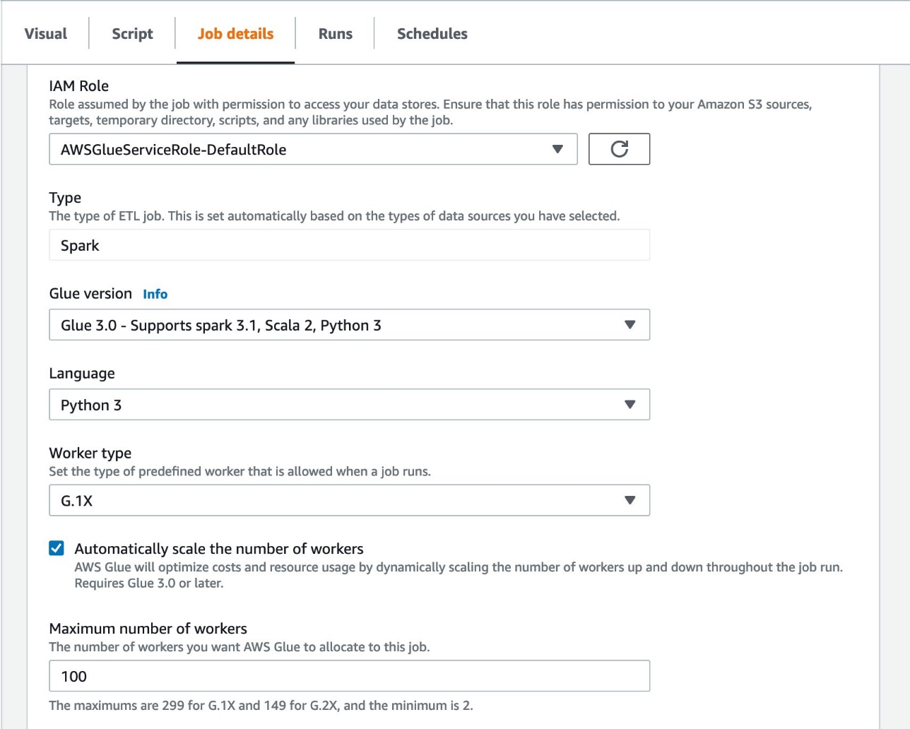
AWS Glue Auto Scaling is available with the optimized Spark runtime on Glue version 3.0. To enable Auto Scaling on the AWS Glue Studio console, complete the following steps:

  1. Open AWS Glue Studio.
  2. Choose Jobs.
  3. Choose your job.
  4. Choose the Job details tab.
  5. For Glue version, choose Glue 3.0 – Supports spark 3.1, Scala 2, Python.
  6. Select Automatically scale the number of workers.
  7. For Maximum number of workers, enter the maximum workers that can be vended to the job run.
  8. Choose Save.

To enable Auto Scaling in the AWS Glue API or AWS Command Line Interface (AWS CLI), set the following job parameters:

  • Key – --enable-auto-scaling
  • Value – true

Monitor AWS Glue Auto Scaling

In this section, we discuss three ways to monitor AWS Glue Auto Scaling: via Amazon CloudWatch metrics or Spark UI.

CloudWatch metrics

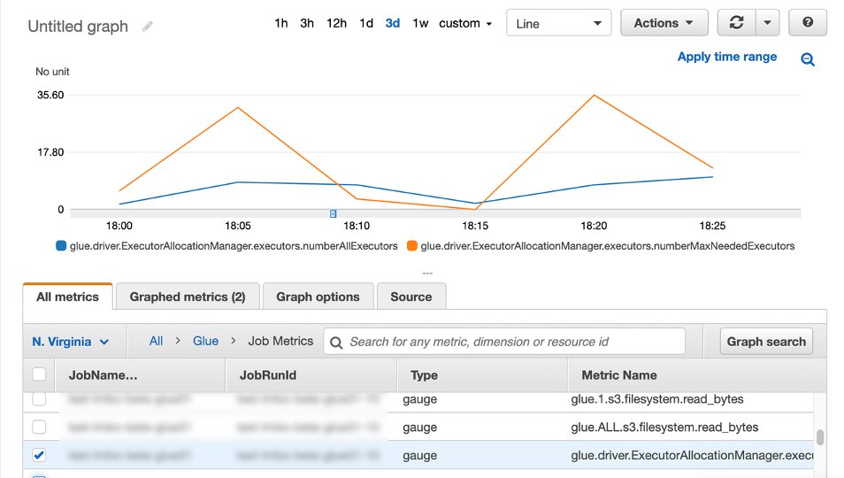
After you enable AWS Glue Auto Scaling, Spark dynamic allocation is enabled and the executor metrics are visible in CloudWatch. You can review the following metrics to understand the demand and optimized usage of executors in their Spark applications enabled with Auto Scaling:

  • glue.driver.ExecutorAllocationManager.executors.numberAllExecutors
  • glue.driver.ExecutorAllocationManager.executors.numberMaxNeededExecutors

AWS Glue Studio Monitoring page

In the Monitoring page in AWS Glue Studio, you can monitor the DPU hours you spent for a specific job run. The following screenshot shows two job runs that processed the same dataset; one without Auto Scaling which spent 8.71 DPU hours, and another one with Auto Scaling enabled which spent only 1.48 DPU hours. The DPU hour values per job run are also available with GetJobRun API responses.

Spark UI

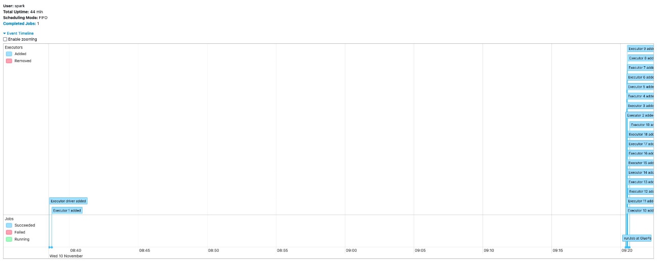
With the Spark UI, you can monitor that the AWS Glue Spark cluster dynamically scales out and scales in with AWS Glue Auto Scaling. The event timeline shows when each executor is added and removed gradually over the Spark application run.

In the following sections, we demonstrate AWS Glue Auto Scaling with two use cases: jobs with driver-heavy workloads, and jobs with multiple stages.

Example 1: Jobs containing driver-heavy workloads

A typical workload for AWS Glue Spark jobs is to process many small files to prepare the data for further analysis. For such workloads, AWS Glue has built-in optimizations, including file grouping, a Glue S3 Lister, partition pushdown predicates, partition indexes, and more. For more information, see Optimize memory management in AWS Glue. All those optimizations execute on the Spark driver and speed up the planning phase on Spark driver to compute and distribute the work for parallel processing with Spark executors. However, without AWS Glue Auto Scaling, Spark executors are idle during the planning phase. With Auto Scaling, Glue jobs only allocate executors when the driver work is complete, thereby saving executor cost.

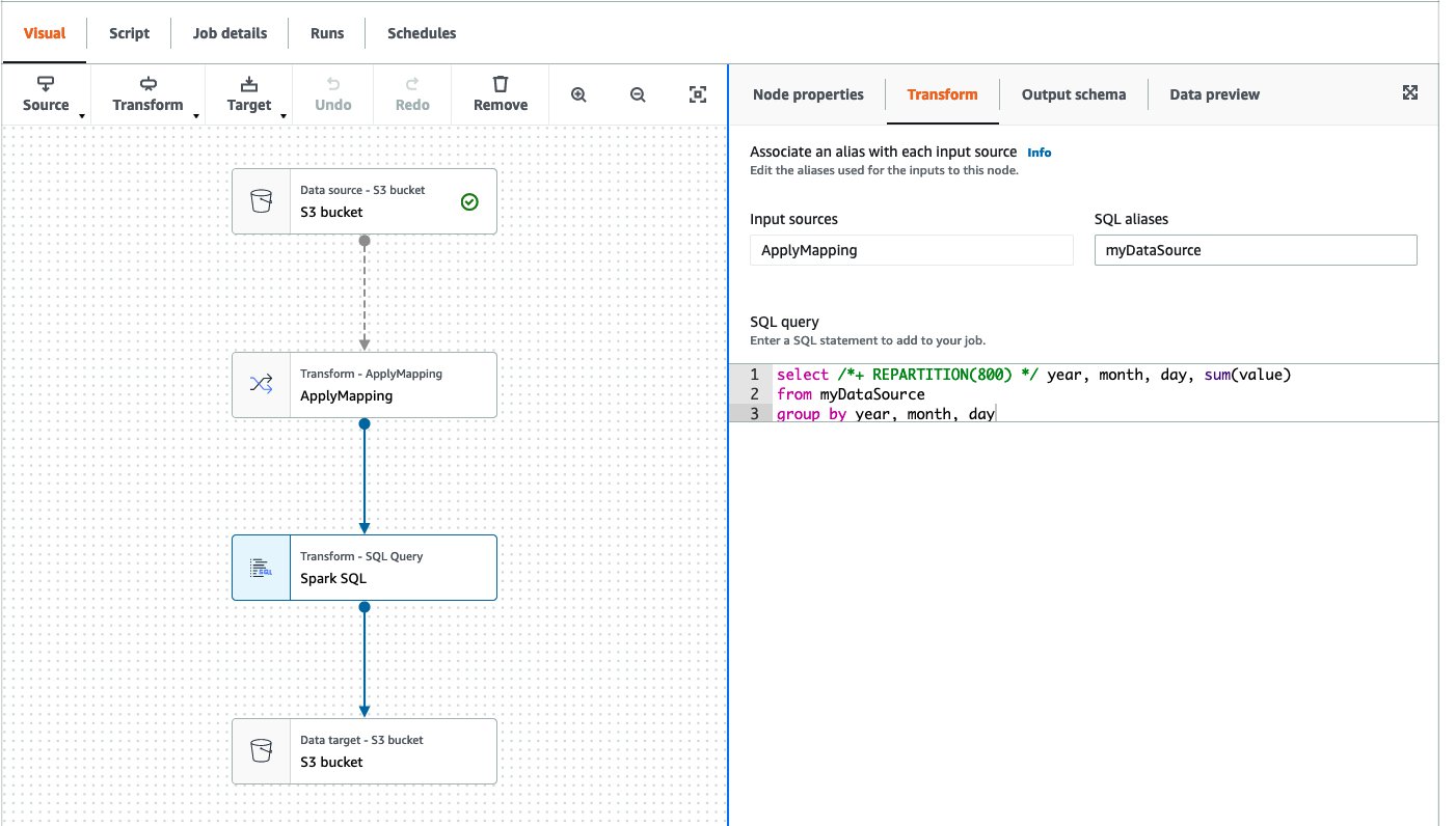
Here’s the example DAG shown in AWS Glue Studio. This AWS Glue job reads from an Amazon Simple Storage Service (Amazon S3) bucket, performs the ApplyMapping transformation, runs a simple SELECT query repartitioning data to have 800 partitions, and writes back to another location in Amazon S3.

Without AWS Glue Auto Scaling

The following screenshot shows the executor timeline in Spark UI when the AWS Glue job ran with 20 workers without Auto Scaling. You can confirm that all 20 workers started at the beginning of the job run.

With AWS Glue Auto Scaling

In contrast, the following screenshot shows the executor timeline of the same job with Auto Scaling enabled and the maximum workers set to 20. The driver and one executor started at the beginning, and other executors started only after the driver finished its computation for listing 367,920 partitions on the S3 bucket. These 19 workers were not charged during the long-running driver task.

Both jobs completed in 44 minutes. With AWS Glue Auto Scaling, the job completed in the same amount of time with lower cost.

Example 2: Jobs containing multiple stages

Another typical workload in AWS Glue is to read from the data store or large compressed files, repartition it to have more parallelism for downstream processing, and process further analytic queries. For example, when you want to read from a JDBC data store, you may not want to have many concurrent connections, so you can avoid impacting source database performance. For such workloads, you can have a small number of connections to read data from the JDBC data store, then repartition the data with higher parallelism for further analysis.

Here’s the example DAG shown in AWS Glue Studio. This AWS Glue job reads from the JDBC data source, runs a simple SELECT query adding one more column (mod_id) calculated from the column ID, performs the ApplyMapping node, then writes to an S3 bucket with partitioning by this new column mod_id. Note that the JDBC data source was already registered in the AWS Glue Data Catalog, and the table has two parameters, hashfield=id and hashpartitions=5, to read from JDBC through five concurrent connections.

Without AWS Glue Auto Scaling

The following screenshot shows the executor timeline in the Spark UI when the AWS Glue job ran with 20 workers without Auto Scaling. You can confirm that all 20 workers started at the beginning of the job run.

With AWS Glue Auto Scaling

The following screenshot shows the same executor timeline in the Spark UI with Auto Scaling enabled with 20 maximum workers. The driver and two executors started at the beginning, and other executors started later. The first two executors read data from the JDBC source with fewer number of concurrent connections. Later, the job increased parallelism and more executors were started. You can also observe that there were 16 executors, not 20, which further reduced cost.

Conclusion

This post discussed AWS Glue Auto Scaling, which automatically resizes the computing resources of your AWS Glue Spark job capacity and reduce cost. You can start using AWS Glue Auto Scaling for both your existing workloads and future new workloads, and take advantage of it today! For more information about AWS Glue Auto Scaling, see Using Auto Scaling for AWS Glue. Migrate your jobs to Glue version 3.0 and get the benefits of Auto Scaling.

Special thanks to everyone who contributed to the launch: Raghavendhar Thiruvoipadi Vidyasagar, Ping-Yao Chang, Shashank Bhardwaj, Sampath Shreekantha, Vaibhav Porwal, and Akash Gupta.


About the Authors

Noritaka Sekiyama is a Principal Big Data Architect on the AWS Glue team. He is passionate about architecting fast-growing data platforms, diving deep into distributed big data software like Apache Spark, building reusable software artifacts for data lakes, and sharing the knowledge in AWS Big Data blog posts. In his spare time, he enjoys taking care of killifish, hermit crabs, and grubs with his children.

Bo Li is a Software Development Engineer on the AWS Glue team. He is devoted to designing and building end-to-end solutions to address customers’ data analytic and processing needs with cloud-based, data-intensive technologies.

Rajendra Gujja is a Software Development Engineer on the AWS Glue team. He is passionate about distributed computing and everything and anything about data.

Mohit Saxena is a Senior Software Development Manager on the AWS Glue team. His team works on distributed systems for efficiently managing data lakes on AWS and optimizes Apache Spark for performance and reliability.

Enhance analytics with Google Trends data using AWS Glue, Amazon Athena, and Amazon QuickSight

Post Syndicated from Drew Philip original https://aws.amazon.com/blogs/big-data/enhance-analytics-with-google-trends-data-using-aws-glue-amazon-athena-and-amazon-quicksight/

In today’s market, business success often lies in the ability to glean accurate insights and predictions from data. However, data scientists and analysts often find that the data they have at their disposal isn’t enough to help them make accurate predictions for their use cases. A variety of factors might alter an outcome and should be taken into account when making a prediction model. Google Trends is an available option, presenting a broad source of data that reflects global trends more comprehensively. This can help enrich a dataset to yield a better model.

You can use Google Trends data for a variety of analytical use cases. For example, you can use it to learn about how your products or brands are faring among targeted audiences. You can also use it to monitor competitors and see how well they’re performing against your brand.

In this post, we shows how to get Google Trends data programmatically, integrate it into a data pipeline, and use it to analyze data, using Amazon Simple Storage Service (Amazon S3), AWS Glue, Amazon Athena, and Amazon QuickSight. We use an example dataset of movies and TV shows and demonstrate how to get the search queries from Google Trends to analyze the popularity of movies and TV shows.

Solution overview

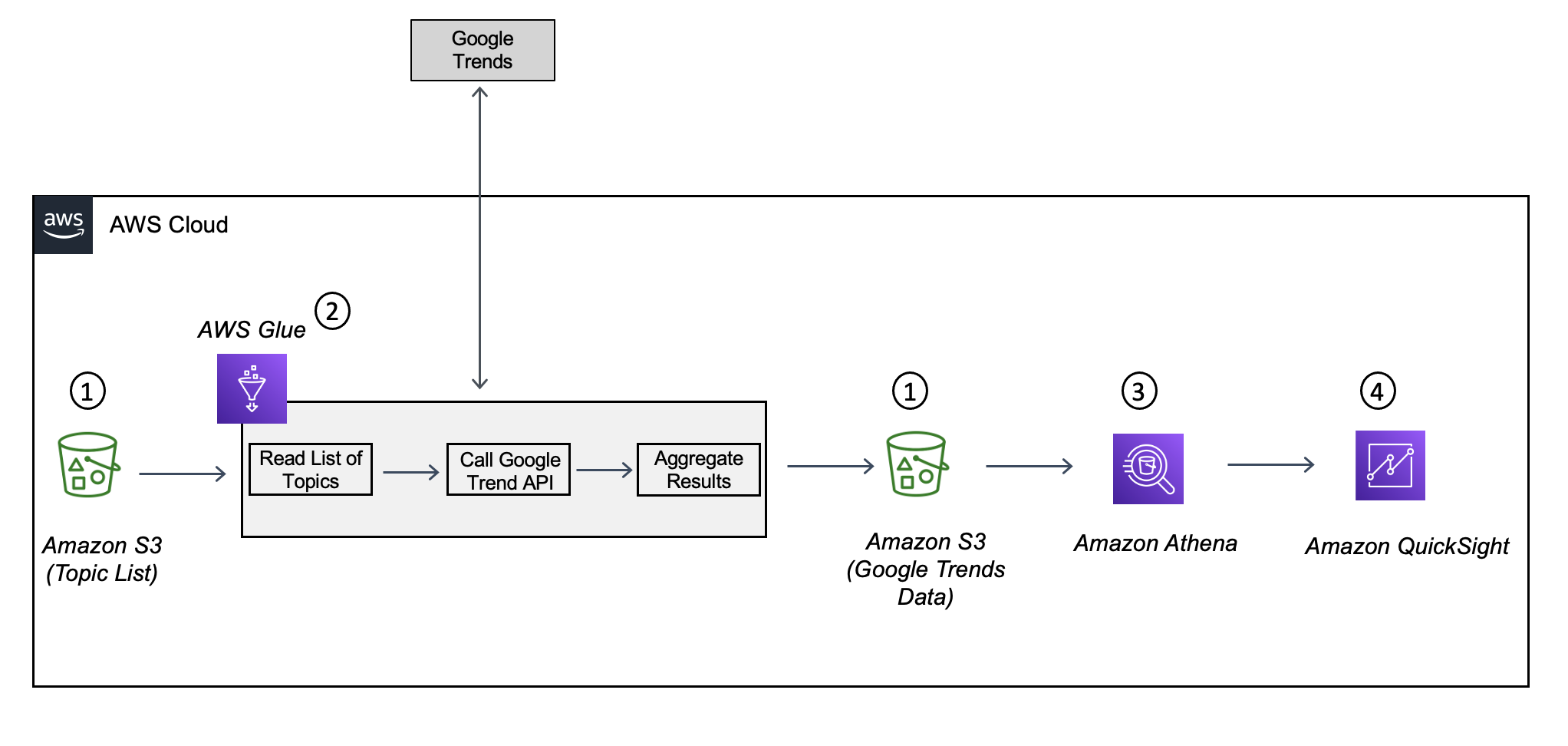
The following diagram shows a high-level architecture of the solution using Amazon S3, AWS Glue, the Google Trends API, Athena, and QuickSight.

The solution consists of the following components:

  1. Amazon S3 – The storage layer that stores the list of topics for which Google Trends data has to be gathered. It also stores the results returned by Google Trends.
  2. AWS Glue – The serverless data integration service that calls Google Trends for the list of topics to get the search results, aggregates the data, and loads it to Amazon S3.
  3. Athena – The query engine that allows you to query the data stored in Amazon S3. You can use it for supporting one-time SQL queries on Google Trends data and for building dashboards using tools like QuickSight.
  4. QuickSight – The reporting tool used for building visualizations.

In the following sections, we walk through the steps to set up the environment, download the libraries, create and run the AWS Glue job, and explore the data.

Set up your environment

Complete the following steps to set up your environment:

  1. Create an S3 bucket where you upload the list of movies and TV shows. For this post, we use a Netflix Movies and TV Shows public dataset from Kaggle.
  2. Create an AWS Identity and Access Management (IAM) service role that allows AWS Glue to read and write data to the S3 buckets you just created.
  3. Create a new QuickSight account with the admin/author role and access granted to Athena and Amazon S3.

Download the external libraries and dependencies for the AWS Glue Job

The AWS Glue job needs the following two external Python libraries: pytrends and awswrangler. pytrends is a library that provides a simple interface for automating the downloading of reports from Google Trends. awswrangler is a library provided by AWS to integrate data between a Pandas DataFrame and AWS repositories like Amazon S3.

Download the following .whl files for the libraries and upload them to Amazon S3:

Create and configure an AWS Glue job

To set up your AWS Glue job, complete the following steps:

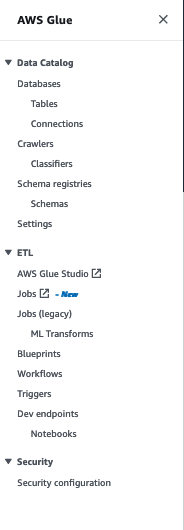
  1. On the AWS Glue console, under ETL in the navigation pane, choose Jobs – New.
  2. For Create job, select Python Shell script editor.
  3. For Options, select Create a new script with boilerplate code.
  4. Choose Create.
  5. On the Script tab, enter the following script, replacing the source and target buckets with your bucket names:
    # Import external library TrendReq needed to connect to Google Trends API and library awswrangler to read/write from pandas to Amazon S3.
    
    from pytrends.request import TrendReq
    pytrend = TrendReq(hl='en-US', tz=360, timeout=10) 
    import pandas as pd
    import awswrangler as wr
    
    # Function get_gtrend, accepts a list of terms as input, calls Google Trends API for each term to get the search trends 
    def get_gtrend(terms):
      trends =[]
      for term in terms:
    # Normalizing the data using popular movie Titanic as baseline to get trends over time.
        pytrend.build_payload(kw_list=["Titanic",term.lower()])
        df = pytrend.interest_over_time()
        df["google_trend"] = round((df[term.lower()] /df['Titanic']) *100)
        
    # Transforming and filtering trends results to align with Analytics use case
        df_trend = df.loc[df.index >= "2018-1-1", "google_trend"].resample(rule="M").max().to_frame()
        df_trend["movie"] = term
        trends.append(df_trend.reset_index())
    
    # Last step in function to concatenate the results for each term and return an aggregated dataset 
      concat_df = pd.concat(trends)
      return concat_df
    
    def main():
      
    # Change the bucket and prefix name to Amazon S3 location where movie titles file from Kaggle has been downloaded. 
      source_bucket = "source_bucket"
      source_prefix = "source_prefix"
    
    # Awswrangler method s3.read_csv is called to load the titles from S3 location into a DataFrame and convert it to a list.
      df = wr.s3.read_csv(f's3://{source_bucket}/{source_prefix}/')
      movies = df['title'].head(20).values.tolist()
    
    #  Call the get_trends function and pass the list of movies as an input. Pandas dataframe is returned with trend data for movies.
      df = get_gtrend(terms=movies)
    
    # Change the prefix name to location where you want to store results. 
      target_bucket = "target_bucket" 
      target_prefix = "target_prefix" 
    
    # Use awswrangler to save pandas dataframe to Amazon S3. 
      wr.s3.to_csv(df,f's3://{target_bucket}/{target_prefix}/trends.csv',index= False)
    
    
    # Invoke the main function
    main()

  6. On the Job details tab, for Name, enter the name of the AWS Glue job.
  7. For IAM Role, choose the role that you created earlier with permissions to run the job and access Amazon S3.
  8. For Type, enter Python Shell to run the Python code.
  9. For Python Version, specify the Python version as Python 3.6.
  10. For Data processing units, choose 1 DPU.
  11. For Number of retries, enter 3­.
  12. Expand Advanced properties and under Libraries, enter the location of the S3 bucket where the pytrends and awswrangler files were downloaded.
  13. Choose Save to save the job.

Run the AWS Glue job

Navigate to the AWS Glue console and run the AWS Glue job you created. When the job is complete, a CSV file with the Google Trends values is created in the target S3 bucket with the prefix specified in the main() function. In the next step, we create an AWS Glue table referring to the target bucket and prefix to allow queries to be run against the Google Trends data.

Create an AWS Glue table on the Google Trends data

In this step, we create a table in the AWS Glue Data Catalog using Athena. The table is created on top of the Google Trends data saved in the target S3 bucket.

In the Athena query editor, select default as the database and enter the following DDL command to create a table named trends. Replace the target bucket and prefix with your own values.

CREATE EXTERNAL TABLE `trends`(
  `date` date, 
  `google_trend` double, 
  `title` string)
ROW FORMAT DELIMITED 
  FIELDS TERMINATED BY ',' 
STORED AS INPUTFORMAT 
  'org.apache.hadoop.mapred.TextInputFormat' 
OUTPUTFORMAT 
  'org.apache.hadoop.hive.ql.io.HiveIgnoreKeyTextOutputFormat'
LOCATION
  's3://<< target_bucket >>/<<target_prefix >>/'
TBLPROPERTIES (
  'has_encrypted_data'='false', 
  'skip.header.line.count'='1')

This table has three columns:

  • date – The time dimension for aggregating the data. In this example, the time period is monthly.
  • google_trend – The count of Google Trends values normalized on a scale of 0–100.
  • title – The name of the movie or TV show.

Query the data using Athena

Now you can run one-time queries to find the popularity of movies and TV shows.

In the first example, we find the top 10 most popular movies and TV shows for November 2021. In the Athena query editor, enter the following SQL command to query the trends table created in the previous step:

select title,google_trend
from trends 
where date = date_parse('2021-11-30','%Y-%m-%d')
order by google_trend desc
limit 10

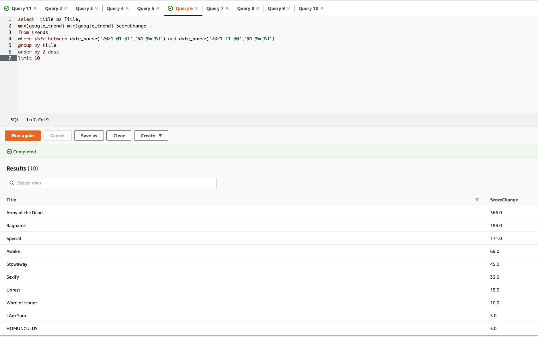
In the following example, we find the top 10 most popular movies and TV shows that have grown most in popularity in 2021 until November 30. In the Athena query editor, enter the following SQL command to query the trends table:

select  title,max(google_trend)-min(google_trend) trend_diff
from trends
where date between date_parse('2021-01-31','%Y-%m-%d') and date_parse('2021-11-30','%Y-%m-%d')
group by title
order by 2 desc
limit 10

Build a dashboard to visualize the data using QuickSight

We can use QuickSight to build a dashboard on the data downloaded from Google Trends to identify top movies and TV shows. Complete the following steps:

  1. Sign in to your QuickSight account.
  2. On the QuickSight console, choose Datasets and choose New dataset.
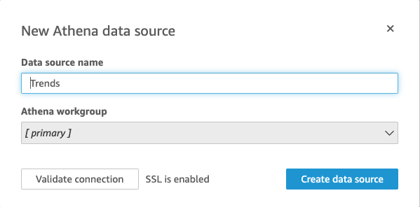
  3. Choose Athena as your data source.
  4. For Data source name, enter a name.
  5. For Athena workgroup, choose [primary].
  6. Choose Create data source.
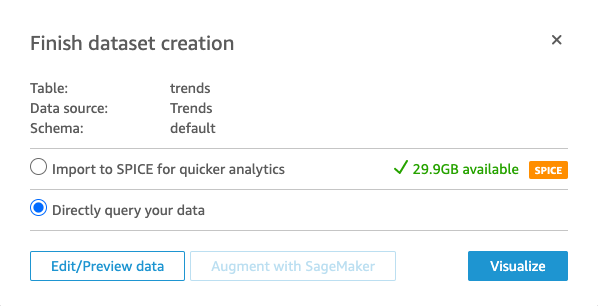
  7. For Database, choose default.
  8. For Tables, select the trends table.
  9. Choose Select.
  10. Select Directly query your data.
  11. Choose Visualize.

For the first visual, we create a bar chart of the top movies or TV shows by title sorted in ascending order of aggregated Google Trends values.

  1. Choose the horizontal bar chart visual type.
  2. For Y axis, choose title.
  3. For Value, choose google_trend (Average).

Next, we create a time series plot of Google Trends count by month for titles.

  1. Add a new visual and choose the autograph visual type.
  2. For X axis, choose date.
  3. For Value, choose google_trend (Sum).
  4. For Color¸ choose title.

Clean up

To avoid incurring future charges, delete the resources you created for AWS Glue, Amazon S3, IAM, and QuickSight.

  1. AWS Glue Catalog table
    • On the AWS Glue console, choose Tables under Databases in the navigation pane.
    • Select the AWS Glue Data Catalog table that you created.
    • On the Actions drop-down menu, choose Delete.
    • Choose Delete to confirm.
  2. AWS Glue Job
    • Choose Jobs in the navigation pane.
    • Select the AWS Glue job you created.
    • On the Actions drop-down menu, choose Delete.
  3. S3 bucket
    • On the Amazon S3 console, choose Buckets in navigation pane.
    • Choose the bucket you created.
    • Choose Empty and enter your bucket name.
    • Choose Confirm.
    • Choose Delete and enter your bucket name.
    • Choose Delete bucket.
  4. IAM Role
    • On the IAM console, choose Roles in navigation pane.
    • Choose the role you attached to AWS Glue job.
    • Choose Delete role.
    • Choose Yes.
  5. Amazon QuickSight
    • If you created a QuickSight user for trying out this blog and do not want to retain that access, please ask your QuickSight admin to delete your user.
    • If you created the QuickSight account itself just for trying this blog and no longer want to retain it, use following steps to delete it.
    • Choose your user name on the application bar, and then choose Manage QuickSight
    • Choose Account settings.
    • Choose Delete Account.

You can only have one QuickSight account active for each AWS account. Make sure that other users aren’t using QuickSight before you delete the account.

Conclusion

Integrating external data sources such as Google Trends via AWS Glue, Athena, and QuickSight can help you enrich your datasets to yield greater insights. You can use it in a data science context when the model is under-fit and requires more relevant data in order to make better predictions. In this post, we used movies as an example, but the solution extends to a wide breadth of industries, such as products in a retail context or commodities in a finance context. If the simple inventory histories or the transaction dates are available, you may find little correlation to future demand or prices. But with an integrated data pipeline using external data, new relationships in the dataset make the model more reliable.

In a business context, whether your team wants to test out a machine learning (ML) proof of concept more quickly or have limited access to pertinent data, Google Trends integration is a relatively quick way to enrich your data for the purposes of ML and data insights.

You can also extend this concept to other third-party datasets, such as social media sentiment, as your team’s expertise grows and your ML and analytics operations mature. Integrating external datasets such as Google Trends is just one part of the feature and data engineering process, but it’s a great place to start and, in our experience, most often leads to better models that businesses can innovate from.


About the Authors

Drew Philip is a Sr. Solutions Architect with AWS Private Equity. He has held senior
technical leadership positions within key AWS partners such as Microsoft, Oracle, and
Rackspace. Drew focuses on applied engineering that leverages AI-enabled digital innovation and development, application modernization, resiliency and operational excellence for workloads at scale in the public and private sector. He sits on the board of Calvin University’s computer science department and is a contributing member of the AWS Machine Learning Technical Focus Community.

Gautam Prothia is a Senior Solution Architect within AWS dedicated to Strategic Accounts. Gautam has more than 15+ years of experience designing and implementing large-scale data management and analytical solutions. He has worked with many clients across industries to help them modernize their data platforms on the cloud.

Simon Zamarin is an AI/ML Solutions Architect whose main focus is helping customers extract value from their data assets. In his spare time, Simon enjoys spending time with family, reading sci-fi, and working on various DIY house projects.

Scale Amazon Redshift to meet high throughput query requirements

Post Syndicated from Erik Anderson original https://aws.amazon.com/blogs/big-data/scale-amazon-redshift-to-meet-high-throughput-query-requirements/

Many enterprise customers have demanding query throughput requirements for their data warehouses. Some may be able to address these requirements through horizontally or vertically scaling a single cluster. Others may have a short duration where they need extra capacity to handle peaks that can be addressed through Amazon Redshift concurrency scaling. However, enterprises with consistently high demand that can’t be serviced by a single cluster need another option. These enterprise customers require large datasets to be returned from queries at a high frequency. These scenarios are also often paired with legacy business intelligence (BI) tools where data is further analyzed.

Amazon Redshift is a fast, fully managed cloud data warehouse. Tens of thousands of customers use Amazon Redshift as their analytics platform. These customers range from small startups to some of the world’s largest enterprises. Users such as data analysts, database developers, and data scientists use Amazon Redshift to analyze their data to make better business decisions.

This post provides an overview of the available scaling options for Amazon Redshift and also shares a new design pattern that enables query processing in scenarios where having multiple leader nodes are required to extract large datasets for clients or BI tools without introducing additional overhead.

Common Amazon Redshift scaling patterns

Because Amazon Redshift is a managed cloud data warehouse, you only pay for what you use, so sizing your cluster appropriately is critical for getting the best performance at the lowest cost. This process begins with choosing the appropriate instance family for your Amazon Redshift nodes. For new workloads that are planning to scale, we recommend starting with our RA3 nodes, which allow you to independently tailor your storage and compute requirements. The RA3 nodes provide three instance types to build your cluster with: ra3.xlplus, ra3.4xlarge, and ra3.16xlarge.

Horizontal cluster scaling

Let’s assume for this example, you build your cluster with four ra3.4xlarge nodes. This configuration provides 48 vCPUs and 384 GiB RAM. Your workload is consistent throughout the day, with few peaks and valleys. As adoption increases and more users need access to the data, you can add nodes of the same node type to your cluster to increase the amount of compute power available to handle those queries. An elastic resize is the fastest way to horizontally scale your cluster to add nodes as a consistent load increases.

Vertical cluster scaling

Horizontal scaling has its limits, however. Each node type has a limit to the number of nodes that can be managed in a single cluster. To continue with the previous example, ra3.4xlarge nodes have a maximum of 64 nodes per cluster. If your workload continues to grow and you’re approaching this limit, you may decide to vertically scale your cluster. Vertically scaling increases the resources given to each node. Based on the additional resources provided by the larger nodes, you will likely decrease the quantity of nodes at the same time.

Rather than running a cluster with 64 ra3.4xlarge nodes, you could elastically resize your cluster to use 16 ra3.16xlarge nodes and have the equivalent resources to host your cluster. The transition to a larger node type allows you to horizontally scale with those larger nodes. You can create an Amazon Redshift cluster with up to 16 nodes. However, after creation, you can resize your cluster to contain up to 32 ra3.xlplus nodes, up to 64 ra3.4xlarge nodes, or up to 128 ra3.16xlarge nodes.

Concurrency scaling

In March 2019, AWS announced the availability of Amazon Redshift concurrency scaling. Concurrency scaling allows you to add more query processing power to your cluster, but only when you need it. Rather than a consistent volume of workload throughout the day, perhaps there are short periods of time when you need more resources. When you choose concurrency scaling, Amazon Redshift automatically and transparently adds more processing power for just those times when you need it. This is a cost-effective, low-touch option for burst workloads. You only pay for what you use on a per-second basis, and you accumulate 1 hour’s worth of concurrency scaling credits every 24 hours. Those free credits have met the needs of 97% of our Amazon Redshift customers’ concurrency scaling requirements, meaning that most customers get the benefits of concurrency scaling without increasing their costs.

The size of your concurrency scaling cluster is directly proportional to your cluster size, so it also scales as your cluster does. By right-sizing your base cluster and using concurrency scaling, you can address the vast majority of performance requirements.

Multi-cluster scaling

Although the previous three scaling options work together to address the needs of the vast majority of our customers, some customers need another option. These use cases require large datasets to be returned from queries at a high frequency and perform further analysis on them using legacy BI tools.

While working with customers to address these use cases, we have found that in these scenarios, multiple medium-sized clusters can perform better than a single large cluster. This phenomenon mostly relates to the single Amazon Redshift leader node’s throughput capacity.

This last scaling pattern uses multiple Amazon Redshift clusters, which allows you to achieve near-limitless read scalability. Rather than relying on a single cluster, a single leader node, and concurrency scaling, this architecture allows you to add as many resources as needed to address your high throughput query requirements. This pattern relies on Amazon Redshift data sharing abilities to enable a seamless multi-cluster experience.

The remainder of this post covers the details of this architecture.

Solution overview

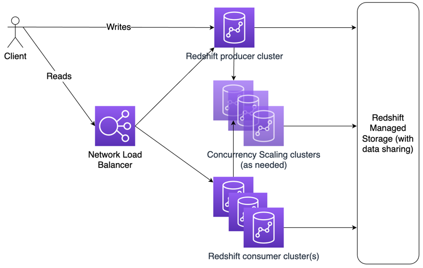
The following diagram outlines a multi-cluster architecture.

The first supporting component for this architecture is Amazon Redshift managed storage. Managed storage is available for RA3 nodes and allows the complete decoupling of compute and storage resources. This decoupling supports another feature that was announced at AWS re:Invent 2020—data sharing. Data sharing is primarily intended to let you share data amongst different data warehouse groups so that you can retain a single set of data to remove duplication. Data sharing ensures that the users accessing the data are using compute on their clusters rather than using compute on the owning cluster, which better aligns cost to usage.

In this post, we introduce another use case of data sharing: horizontal cluster scaling. This architecture allows you to create two or more clusters to handle high throughput query requirements while maintaining a single data source.

An important component in this design is the Network Load Balancer (NLB). The NLB serves as a single access point for clients to connect to the backend data warehouse for performing reads. It also allows changing the number of underlying clusters transparently to users. If you decide to add or remove clusters, all you need to do is add or remove targets in your NLB. It’s also important to note that this design can use any of the previous three scaling options (horizontal, vertical, and concurrency scaling) to fine-tune the number of resources available to service your particular workload.

Prerequisites

Let’s start by creating two Amazon Redshift clusters of RA3 instance type, and name them producer_cluster and consumer_cluster. For instructions, refer to Create a cluster.

In this post, our producer cluster is a central ETL cluster hosting enterprise sales data using a 3 TB Cloud DW dataset based on the TPC-DS benchmark.

The next step is to configure data sharing between the producer and consumer clusters.

Set up data sharing at the producer cluster

In this step, you need a cluster namespace from the consumer_cluster. One way to find the namespace value of a cluster is to run the SQL statement SELECT CURRENT_NAMESPACE when connected to the consumer_cluster. Another way is through the Amazon Redshift console. Navigate to your Amazon Redshift consumer_cluster, and find the cluster namespace located in the General information section.

After you connect to the producer cluster, create the data share and add the schema and tables to the data share. Then, grant usage to the consumer namespace by providing the namespace value. See the following code:

/* Create Datashare and add objects to the share */ 
CREATE DATASHARE producertpcds3tb;

ALTER DATASHARE producertpcds3tb ADD SCHEMA order_schema;
ALTER DATASHARE producertpcds3tb ADD ALL TABLES in SCHEMA order_schema;

GRANT USAGE ON DATASHARE producertpcds3tb TO NAMESPACE '<consumer namespace>';

You can validate that data sharing was correctly configured by querying these views from the producer cluster:

SELECT * FROM SVV_DATASHARES;
SELECT * FROM SVV_DATASHARE_OBJECTS;

Set up data sharing at the consumer cluster

Get the cluster namespace of the producer cluster by following same steps for the consumer cluster. After you connect to the consumer cluster, you can create a database referencing the data share of the producer cluster. Then you create an external schema and set the search path in the consumer cluster, which allows schema-level access control within the consumer cluster and uses a two-part notation when referencing shared data objects. Finally, you grant usage on the database to a user, and run a query to check if objects as part of data share are accessible. See the following code:

/* Create a local database and schema reference */

CREATE DATABASE tpcds_3tb FROM DATASHARE producertpcds3tb OF NAMESPACE '<producer namespace>';


/*Create External schema */
CREATE EXTERNAL SCHEMA order_schema FROM REDSHIFT DATABASE 'tpcds_3tb' SCHEMA 'order_schema';

SET SEARCH_PATH TO order_schema,public;


/* Grant usage on database to a user */ 

GRANT USAGE On DATABASE tpcds_3tb TO awsuser;

/* Query to check objects accessible from the consumer cluster */

SELECT * FROM SVV_DATASHARE_OBJECTS;

Set up the Network Load Balancer

After you set up data sharing at both the producer_cluster and consumer_cluster, the next step is to configure a Network Load Balancer to accept connections through a single endpoint and forward the connections to both clusters for reading data via queries.

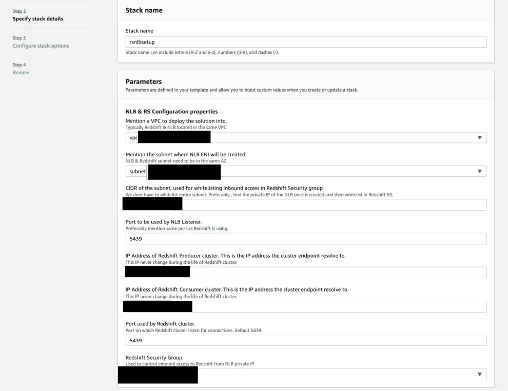
As a prerequisite, collect the following information from the Amazon Redshift producer and consumer clusters on the Amazon Redshift console in the cluster properties section. Use the producer cluster information if consumer cluster is not mentioned below.

Parameter Name Parameter Description
VPCid Amazon Redshift cluster VPC
NLBSubnetid Subnet where the NLB ENI is created. The NLB and Amazon Redshift subnet need to be in the same Availability Zone.
NLBSubnetCIDR Used for allowlisting inbound access in the Amazon Redshift security group
NLBPort Port to be used by NLB Listener, usually the same port as Amazon Redshift port 5439
RedshiftPrivateIP IP address of Amazon Redshift leader node of the producer cluster
RedshiftPrivateIP IP address of Amazon Redshift leader node of the consumer cluster
RedshiftPort: Port used by Amazon Redshift clusters, usually 5439
RedshiftSecurityGroup Security group to allow connectivity to Amazon Redshift cluster

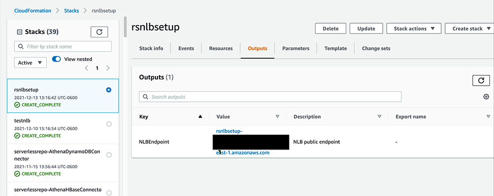
After you collect this information, run the AWS CloudFormation script NLB.yaml to set up the Network Load Balancer for the producer and consumer clusters. The following screenshot shows the stack parameters.

After you create the CloudFormation stack, note the NLB endpoint on the stack’s Outputs tab. You use this endpoint to connect to the Amazon Redshift clusters.

This NLB setup is done for the both producer and consumer clusters by the CloudFormation stack. If needed, you can add additional Amazon Redshift clusters to an existing NLB by navigating to Target groups page of the Amazon EC2 console. Then navigate to rsnlbsetup-target and add the Amazon Redshift cluster leader node private IP and port.

Validate the connections to the Amazon Redshift clusters

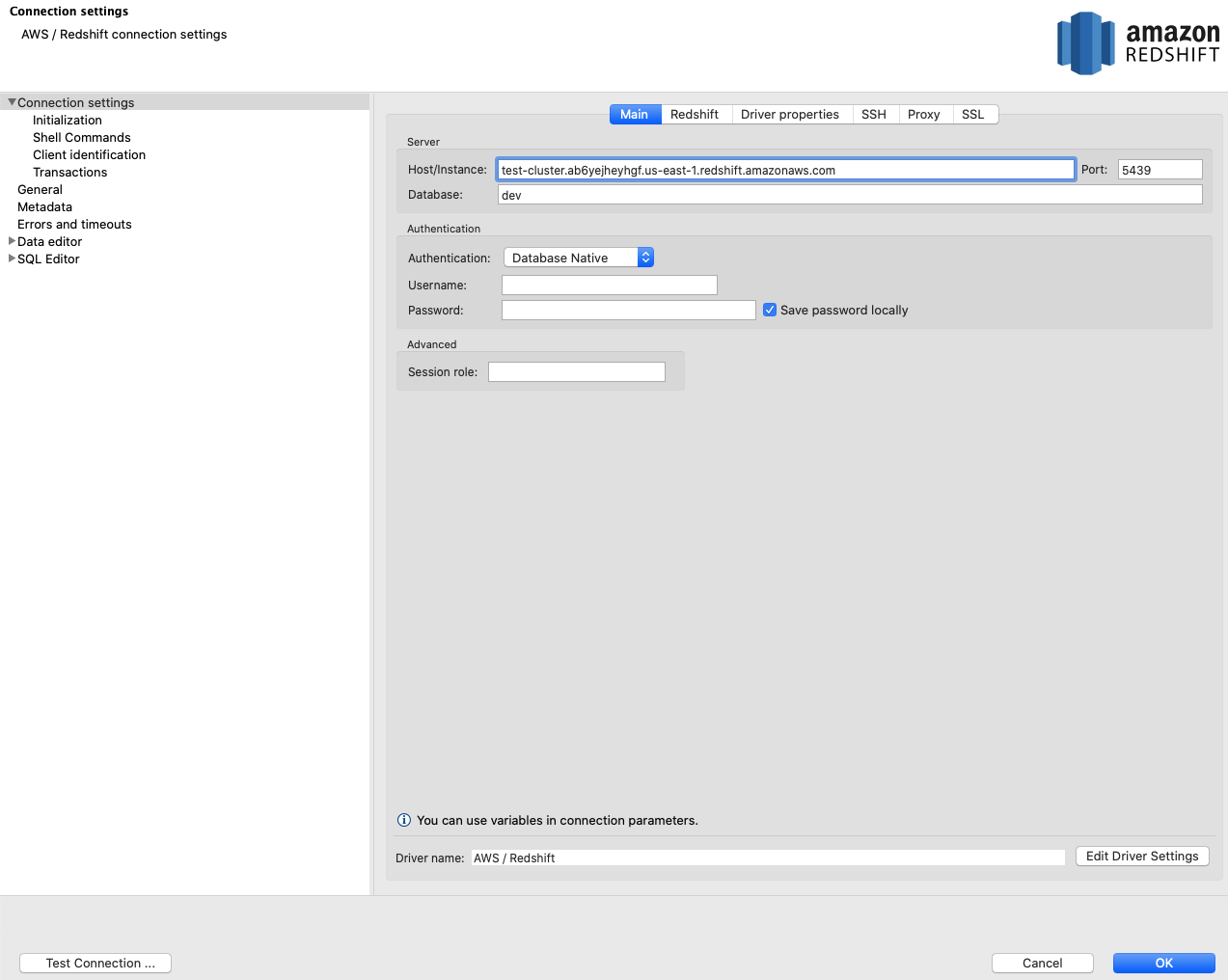
After you set up the NLB, the next step is to validate the connectivity to the Amazon Redshift clusters. You can do this by first configuring SQL tools like SQL Workbench, DBeaver, or Aginity Workbench and setting the host name and endpoint to the Amazon Redshift cluster’s NLB endpoint, as shown in the following screenshot. For additional configuration information, see Connecting to an Amazon Redshift cluster using SQL client tools.

Repeat this process a few times to validate that there are connections to both clusters. Similarly, you can use the same NLB endpoint as the host name while configuring.

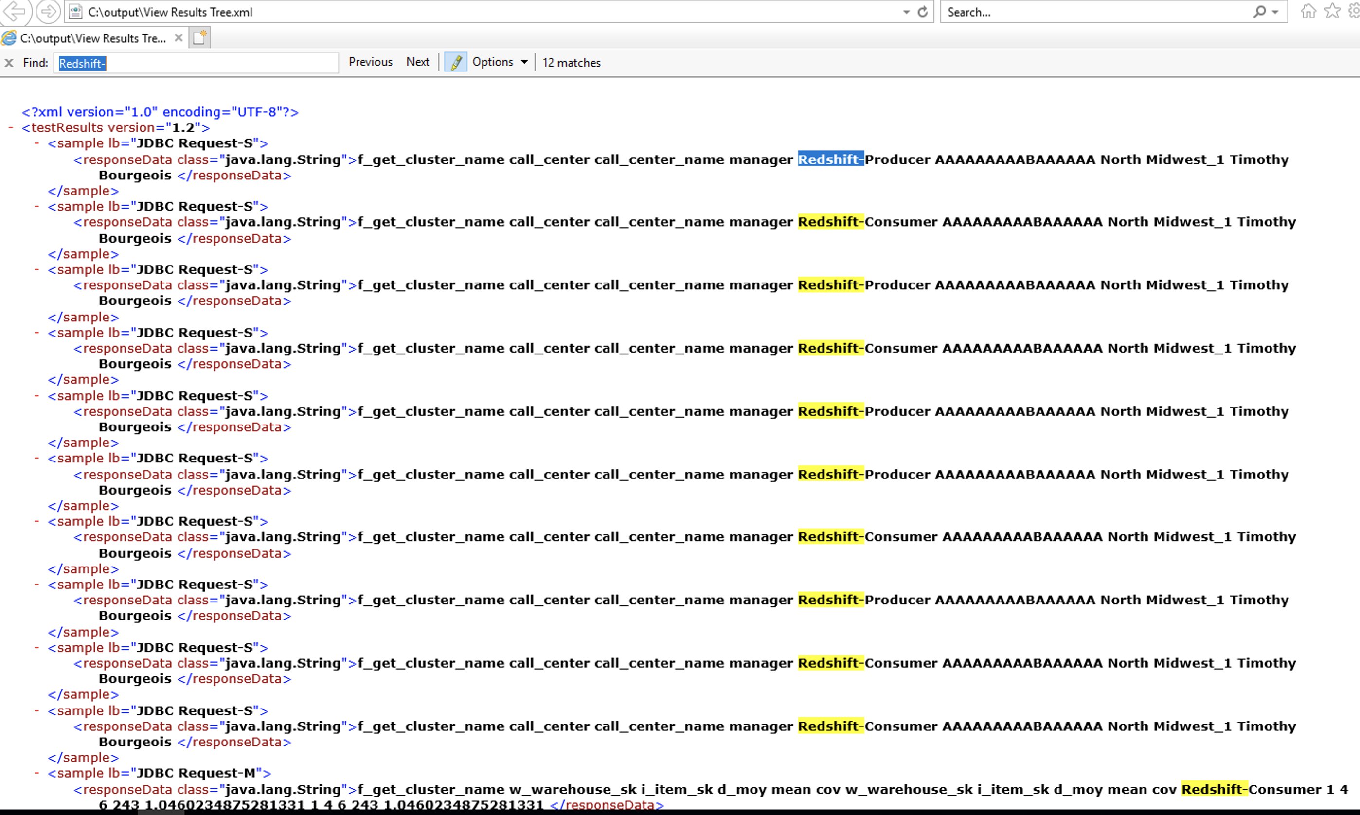
As a next step, we use JMeter to show how the NLB is connecting to each of the clusters. The Apache JMeter application is open-source software, a 100% pure Java application designed to load test functional behavior and measure performance. Our NLB connects to each cluster in a round-robin manner, which enables even distribution of read load on Amazon Redshift clusters.

Setting up JMeter is out of scope of this post; refer to Building high-quality benchmark tests for Amazon Redshift using Apache JMeter to learn more about setting up JMeter and performance testing on an Amazon Redshift cluster.

The following screenshot shows the HTML output of the response data from JMeter testing. It shows that requests go to both the Amazon Redshift producer and consumer clusters in a round-robin manner.

The preceding screenshot shows a sample output from running 20 SQL queries. Testing with over 1,000 SQL runs was performed with over four Amazon Redshift clusters, and the NLB was able to distribute them as evenly as possible across all of those clusters.

With this setup, you have the flexibility to add Amazon Redshift clusters to your NLB as needed and can configure data sharing to enable horizontal scaling of Amazon Redshift clusters. When demand reduces, you can either de-register some of the Amazon Redshift clusters at the NLB configuration or simply pause the Amazon Redshift cluster and the NLB automatically connects to only those clusters that are available at the time.

Conclusion

In this post, you learned about the different ways that Amazon Redshift can scale to meet your needs as they adjust over time. Use horizontal scaling to increase the number of nodes in your cluster. Use vertical scaling to increase the size of each node. Use concurrency scaling to dynamically address peak workloads. Use multiple clusters with data sharing behind an NLB to provide near-endless scalability. You can use these architectures independently or in combination with each other to build your high-performing, cost-effective data warehouse using Amazon Redshift.

To learn more about some of the foundational features used in the architecture mentioned in this post, refer to:


About the Authors

Erik Anderson is a Principal Solutions Architect at AWS. He has nearly two decades of experience guiding numerous Fortune 100 companies along their technology journeys. He is passionate about helping enterprises build scalable, performant, and cost-effective solutions in the cloud. In his spare time, he loves spending time with his family, home improvement projects, and playing sports.

Rohit Bansal is a Analytics Specialist Solutions Architect at AWS. He specializes in Amazon Redshift and works with customers to build next-generation Analytics solutions using other AWS Analytics Services.

Amazon Redshift continues its price-performance leadership

Post Syndicated from Stefan Gromoll original https://aws.amazon.com/blogs/big-data/amazon-redshift-continues-its-price-performance-leadership/

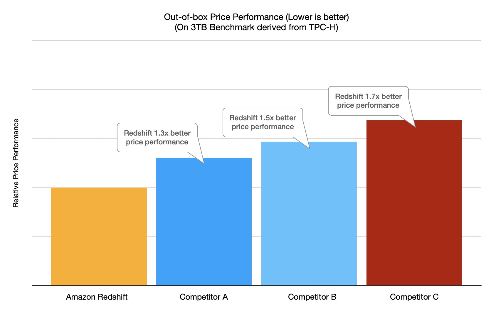
Data is a strategic asset. Getting timely value from data requires high-performance systems that can deliver performance at scale while keeping costs low. Amazon Redshift is the most popular cloud data warehouse that is used by tens of thousands of customers to analyze exabytes of data every day. We continue to add new capabilities to improve the price-performance ratio for our customers as you bring more data to your Amazon Redshift environments.

This post goes into detail on the analytic workload trends we’re seeing from the Amazon Redshift fleet’s telemetry data, new capabilities we have launched to improve Amazon Redshift’s price-performance, and the results from the latest benchmarks derived from TPC-DS and TPC-H, which reenforce our leadership.

Data-driven performance optimization

We relentlessly focus on improving Amazon Redshift’s price-performance so that you continue to see improvements in your real-world workloads. To this end, the Amazon Redshift team takes a data-driven approach to performance optimization. Werner Vogels discussed our methodology in Amazon Redshift and the art of performance optimization in the cloud, and we have continued to focus our efforts on using performance telemetry from our large customer base to drive the Amazon Redshift performance improvements that matter most to our customers.

At this point, you might ask why does price-performance matter? One critical aspect of a data warehouse is how it scales as your data grows. Will you be paying more per TB as you add more data, or will your costs remain consistent and predictable? We work to make sure that Amazon Redshift delivers not only strong performance as your data grows, but also consistent price-performance.

Optimizing high-concurrency, low-latency workloads

One of the trends that we have observed is that customers are increasingly building analytics applications that require high concurrency of low-latency queries. In the context of data warehousing, this can mean hundreds or even thousands of users running queries with response time SLAs of under 5 seconds.

A common scenario is an Amazon Redshift-powered business intelligence dashboard that serves analytics to a very large number of analysts. For example, one of our customers processes foreign exchange rates and delivers insights based on this data to their users using an Amazon Redshift-powered dashboard. These users generate an average of 200 concurrent queries to Amazon Redshift that can spike to 1,200 concurrent queries at the open and close of the market, with a P90 query SLA of 1.5 seconds. Amazon Redshift is able to meet this requirement, so this customer can meet their business SLAs and provide the best service possible to their users.

A specific metric we track is the percentage of runtime across all clusters that is spent on short-running queries (queries with runtime less than 1 second). Over the last year, we’ve seen a significant increase in short query workloads in the Amazon Redshift fleet, as shown in the following chart.

As we started to look deeper into how Amazon Redshift ran these kinds of workloads, we discovered several opportunities to optimize performance to give you even better throughput on short queries:

  • We significantly reduced Amazon Redshift’s query-planning overhead. Even though this isn’t large, it can be a significant portion of the runtime of short queries.
  • We improved the performance of several core components for situations where many concurrent processes contend for the same resources. This further reduced our query overhead.
  • We made improvements that allowed Amazon Redshift to more efficiently burst these short queries to concurrency scaling clusters to improve query parallelism.

To see where Amazon Redshift stood after making these engineering improvements, we ran an internal test using the Cloud Data Warehouse Benchmark derived from TPC-DS (see a later section of this post for more details on the benchmark, which is available in GitHub). To simulate a high-concurrency, low-latency workload, we used a small 10 GB dataset so that all queries ran in a few seconds or less. We also ran the same benchmark against several other cloud data warehouses. We didn’t enable auto scaling features such as concurrency scaling on Amazon Redshift for this test because not all data warehouses support it. We used an ra3.4xlarge Amazon Redshift cluster, and sized all other warehouses to the closest matching price-equivalent configuration using on-demand pricing. Based on this configuration, we found that Amazon Redshift can deliver up to 8x better performance on analytics applications that predominantly required short queries with low latency and high concurrency, as shown in the following chart.

With Concurrency Scaling on Amazon Redshift, throughput can be seamlessly and automatically scaled to additional Amazon Redshift clusters as user concurrency grows. We increasingly see customers using Amazon Redshift to build such analytics applications based on our telemetry data.

This is just a small peek into the behind-the-scenes engineering improvements our team is continually making to help you improve performance and save costs using a data-driven approach.

New features improving price-performance

With the constantly evolving data landscape, customers want high-performance data warehouses that continue to launch new capabilities to deliver the best performance at scale while keeping costs low for all workloads and applications. We have continued to add features that improve Amazon Redshift’s price-performance out of the box at no additional cost to you, allowing you to solve business problems at any scale. These features include the use of best-in-class hardware through the AWS Nitro System, hardware acceleration with AQUA, auto-rewriting queries so that they run faster using materialized views, Automatic Table Optimization (ATO) for schema optimization, Automatic Workload Management (WLM) to offer dynamic concurrency and optimize resource utilization, short query acceleration, automatic materialized views, vectorization and single instruction/multiple data (SIMD) processing, and much more. Amazon Redshift has evolved to become a self-learning, self-tuning data warehouse, abstracting away the performance management effort needed so you can focus on high-value activities like building analytics applications.

To validate the impact of the latest Amazon Redshift performance enhancements, we ran price-performance benchmarks comparing Amazon Redshift with other cloud data warehouses. For these tests, we ran both a TPC-DS-derived benchmark and a TPC-H-derived benchmark using a 10-node ra3.4xlarge Amazon Redshift cluster. To run the tests on other data warehouses, we chose warehouse sizes that most closely matched the Amazon Redshift cluster in price ($32.60 per hour), using published on-demand pricing for all data warehouses. Because Amazon Redshift is an auto-tuning warehouse, all tests are “out of the box,” meaning no manual tunings or special database configurations are applied—the clusters are launched and the benchmark is run. Price-performance is then calculated as cost per hour (USD) times the benchmark runtime in hours, which is equivalent to the cost to run the benchmark.

For both the TPC-DS-derived and TPC-H-derived tests, we find that Amazon Redshift consistently delivers the best price-performance. The following chart shows the results for the TPC-DS-derived benchmark.

The following chart shows the results for the TPC-H-derived benchmark.

Although these benchmarks reaffirm Amazon Redshift’s price-performance leadership, we always encourage you to try Amazon Redshift using your own proof-of-concept workloads as the best way to see how Amazon Redshift can meet your data needs.

Find the best price-performance for your workloads

The benchmarks used in this post are derived from the industry-standard TPC-DS and TPC-H benchmarks, and have the following characteristics:

  • The schema and data are used unmodified from TPC-DS and TPC-H.
  • The queries are used unmodified from TPC-DS and TPC-H. TPC-approved query variants are used for a warehouse if the warehouse doesn’t support the SQL dialect of the default TPC-DS or TPC-H query.
  • The test includes only the 99 TPC-DS and 22 TPC-H SELECT queries. It doesn’t include maintenance and throughput steps.
  • Three power runs (single stream) were run with query parameters generated using the default random seed of the TPC-DS and TPC-H kits.
  • The primary metric of total query runtime is used when calculating price-performance. The runtime is taken as the best of the three runs.
  • Price-performance is calculated as cost per hour (USD) times the benchmark runtime in hours, which is equivalent to cost to run the benchmark. Published on-demand pricing is used for all data warehouses.

We call this benchmark the Cloud Data Warehouse Benchmark, and you can easily reproduce the preceding benchmark results using the scripts, queries, and data available on GitHub. It is derived from the TPC-DS and TPC-H benchmarks as described earlier, and as such is not comparable to published TPC-DS or TPC-H results, because the results of our tests don’t comply with the specification.

Each workload has unique characteristics, so if you’re just getting started, a proof of concept is the best way to understand how Amazon Redshift performs for your requirements. When running your own proof of concept, it’s important to focus on the right metrics—query throughput (number of queries per hour) and price-performance. You can make a data-driven decision by running a proof of concept on your own or with assistance from AWS or a system integration and consulting partner.

Conclusion

This post discussed the analytic workload trends we’re seeing from Amazon Redshift customers, new capabilities we have launched to improve Amazon Redshift’s price-performance, and the results from the latest benchmarks.

If you’re an existing Amazon Redshift customer, connect with us for a free optimization session and briefing on the new features announced at AWS re:Invent 2021. To stay up to date with the latest developments in Amazon Redshift, follow the What’s New in Amazon Redshift feed.


About the Authors

Stefan Gromoll is a Senior Performance Engineer with Amazon Redshift where he is responsible for measuring and improving Redshift performance. In his spare time, he enjoys cooking, playing with his three boys, and chopping firewood.

Ravi Animi is a Senior Product Management leader in the Redshift Team and manages several functional areas of the Amazon Redshift cloud data warehouse service including performance, spatial analytics, streaming ingestion and migration strategies. He has experience with relational databases, multi-dimensional databases, IoT technologies, storage and compute infrastructure services and more recently as a startup founder using AI/deep learning, computer vision, and robotics.

Florian Wende is a Performance Engineer with Amazon Redshift.

Automate notifications on Slack for Amazon Redshift query monitoring rule violations

Post Syndicated from Dipankar Kushari original https://aws.amazon.com/blogs/big-data/automate-notifications-on-slack-for-amazon-redshift-query-monitoring-rule-violation/

In this post, we walk you through how to set up automatic notifications of query monitoring rule (QMR) violations in Amazon Redshift to a Slack channel, so that Amazon Redshift users can take timely action.

Amazon Redshift is a fully managed, petabyte-scale data warehouse service in the cloud. With Amazon Redshift, you can analyze your data to derive holistic insights about your business and your customers. One of the challenges is to protect the data warehouse workload from poorly written queries that can consume significant resources. Amazon Redshift query monitoring rules are a feature of workload management (WLM) that allow automatic handling of poorly written queries. Rules that are applied to a WLM queue allow queries to be logged, canceled, hopped (only available with manual WLM), or to change priority (only available with automatic WLM). The reason to use QMRs is to protect against wasteful use of the cluster. You can also use these rules to log resource-intensive queries, which provides the opportunity to establish governance for ad hoc workloads.

The Amazon Redshift cluster automatically collects query monitoring rules metrics. This convenient mechanism lets you view attributes like the following:

  • Query runtime, in seconds
  • Query return row count
  • The CPU time for a SQL statement

It also makes Amazon Redshift Spectrum metrics available, such as the number of Redshift Spectrum rows and MBs scanned by a query.

When a query violates a QMR, Amazon Redshift logs the violation into the STL_WLM_RULE_ACTION system view. If the action is aborted for the queries that violate a QMR, end-users see an error that indicates query failure due to violation of QMRs. We recommend that administrative team members periodically examine violations listed in the STL_WLM_RULE_ACTION table and coach the involved end-users on how to avoid future rule violations.

Alternately, a centralized team, using a Slack channel for collaboration and monitoring, can configure Amazon Redshift events and alarms to be sent to their channel, so that they can take timely action. In the following sections, we walk you through how to set up automatic notifications of QMR violations to a Slack channel through the use of Slack events and alarms. This allows Amazon Redshift users to be notified and take timely actions without the need to query the system view.

Solution overview

To demonstrate how you can receive automatic notification to a Slack channel for QMR violation, we have designed the following architecture. As shown in the following diagram, we have mixed workload extract, transform, and load (ETL), business intelligence (BI) dashboards, and analytics applications that are powered by an Amazon Redshift cluster. The solution relies on AWS Lambda and Amazon Simple Notification Service (Amazon SNS) to send notifications of Amazon Redshift QMR violations to Slack.

To implement this solution, you create an Amazon Redshift cluster and attach a custom defined parameter group.

Amazon Redshift provides one default parameter group for each parameter group family. The default parameter group has preset values for each of its parameters, and it can’t be modified. If you want to use different parameter values than the default parameter group, you must create a custom parameter group and then associate your cluster with it.

In the parameter group, you can use automatic WLM and define a few workload queues, such as a queue for processing ETL workloads and a reporting queue for user queries. You can name the default queue adhoc. With automatic WLM, Amazon Redshift determines the optimal concurrency and memory allocation for each query that is running in each queue.

For each workload queue, you can define one or more QMRs. For example, you can create a rule to abort a user query if it runs for more than 300 seconds or returns more than 1 billion rows. Similarly, you can create a rule to log a Redshift Spectrum query that scans more than 100 MB.

The Amazon Redshift WLM evaluates metrics every 10 seconds. It records details about actions that result from QMR violation that is associated with user-defined queues in the STL_WLM_RULE_ACTION system table. In this solution, a Lambda function is scheduled to monitor the STL_WLM_RULE_ACTION system table every few minutes. When the function is invoked, if it finds a new entry, it publishes a detailed message to an SNS topic. A second Lambda function, created as the target subscriber to the SNS topic, is invoked whenever any message is published to the SNS topic. This second function invokes a pre-created Slack webhook, which sends the message that was received through the SNS topic to the Slack channel of your choice. (For more information on publishing messages by using Slack webhooks, see Sending messages using incoming webhooks.)

To summarize, the solution involves the following steps:

  1. Create an Amazon Redshift custom parameter group and add workload queues.
  2. Configure query monitoring rules.
  3. Attach the custom parameter group to the cluster.
  4. Create a SNS topic.
  5. Create a Lambda function and schedule it to run every 5 minutes by using an Amazon EventBridge rule.
  6. Create the Slack resources.
  7. Add an incoming webhook and authorize the Slack app to post messages to a Slack channel.
  8. Create the second Lambda function and subscribe to the SNS topic.
  9. Test the solution.

Create an Amazon Redshift custom parameter group and add workload queues

In this step, you create an Amazon Redshift custom parameter group with automatic WLM enabled. You also create the following queues to separate the workloads in the parameter group:

  • reporting – The reporting queue runs BI reporting queries that are performed by any user who belongs to the Amazon Redshift database group named reporting_group
  • adhoc – The default queue, renamed adhoc, performs any query that is not sent to any other queue

Complete the following steps to create your parameter group and add workload queues:

  1. Create a parameter group, named csblog, with automatic WLM enabled.
  2. On the Amazon Redshift console, select the custom parameter group you created.
  3. Choose Edit workload queues.
  4. On the Modify workload queues page, choose Add queue.
  5. Fill in the Concurrency scaling mode and Query priority fields as needed to create the reporting queue.
  6. Repeat these steps to add the adhoc queue.

For more information about WLM queues, refer to Configuring workload management.

Configure query monitoring rules

In this step, you add QMRs to each workload queue. For instructions, refer to Creating or modifying a query monitoring rule using the console.

For the reporting queue, add the following QMRs:

  • nested_loop – Logs any query involved in a nested loop join that results in a row count more than 10,000,000 rows.
  • long_running – Stops queries that run for more than 300 seconds (5 minutes).

For the adhoc queue, add the following QMRs:

  • returned_rows – Stops any query that returns more than 1,000,000 rows back to the calling client application (this isn’t practical and can degrade the end-to-end performance of the application).
  • spectrum_scan – Stops any query that scans more than 1000 MB of data from an Amazon Simple Storage Service (Amazon S3) data lake by using Redshift Spectrum.

Attach the custom parameter group to the cluster

To attach the custom parameter group to your provisioned Redshift cluster, follow the instructions in Associating a parameter group with a cluster. If you don’t already have a provisioned Redshift cluster, refer to Create a cluster.

For this post, we attached our custom parameter group csblog to an already created provisioned Amazon Redshift cluster.

Create an SNS topic

In this step, you create an SNS topic that receives a detailed message of QMR violation from the Lambda function that checks the Amazon Redshift system table for QMR violation entries. For instructions, refer to Creating an Amazon SNS topic.

For this post, we created an SNS topic named redshiftqmrrulenotification.

Create a Lambda function to monitor the system table

In this step, you create a Lambda function that monitors the STL_WLM_RULE_ACTION system table. Whenever any record is found in the table since the last time the function ran, the function publishes a detailed message to the SNS topic that you created earlier. You also create an EventBridge rule to invoke the function every 5 minutes.

For this post, we create a Lambda function named redshiftqmrrule that is scheduled to run every 5 minutes via an EventBridge rule named Redshift-qmr-rule-Lambda-schedule. For instructions, refer to Building Lambda functions with Python.

The following screenshot shows the function that checks the pg_catalog.stl_wlm_rule_action table.

To create an EventBridge rule and associate it with the Lambda function, refer to Create a Rule.

The following screenshot shows the EventBridge rule Redshift-qmr-rule-Lambda-schedule, which calls the function every 5 minutes.

We use the following Python 3.9 code for this Lambda function. The function uses an Amazon Redshift Data API call that uses GetClusterCredentials for temporary credentials.

import json
import time
import unicodedata
import traceback
import sys
from pip._internal import main
import urllib3
import os
import boto3
from datetime import datetime

# initiate redshift-data client in boto3
client = boto3.client("redshift-data")

query = "select userid,query,service_class,trim(rule) as rule,trim(action) as action,recordtime from stl_wlm_rule_action WHERE userid > 1 AND recordtime >= current_timestamp AT TIME ZONE 'UTC' - INTERVAL '5 minute' order by recordtime desc;"
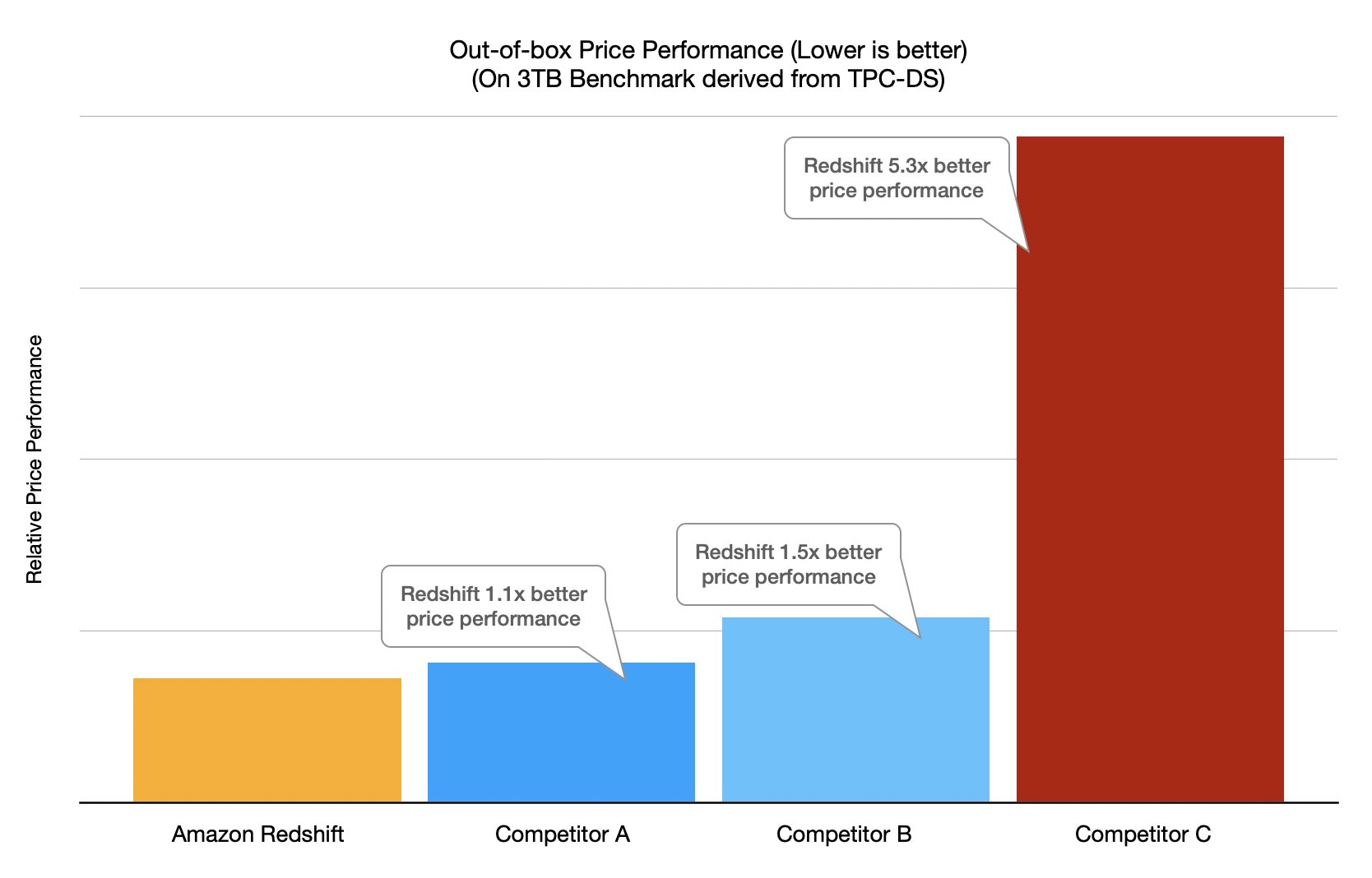
sns = boto3.resource('sns')
sns_arn = os.environ['sns_arn']
platform_endpoint = sns.PlatformEndpoint('{sns_arn}'.format(sns_arn = sns_arn))

def status_check(client, query_id):
    desc = client.describe_statement(Id=query_id)
    status = desc["Status"]
    if status == "FAILED":
        raise Exception('SQL query failed:' + query_id + ": " + desc["Error"])
    return status.strip('"')

def execute_sql(sql_text, redshift_database, redshift_user, redshift_cluster_id):
    print("Executing: {}".format(sql_text))
    res = client.execute_statement(Database=redshift_database, DbUser=redshift_user, Sql=sql_text,
                                   ClusterIdentifier=redshift_cluster_id)
    
    query_id = res["Id"]
    print("query id")
    print(query_id)
    done = False
    while not done:
        time.sleep(1)
        status = status_check(client, query_id)
        if status in ("FAILED", "FINISHED"):
            print("status is: {}".format(status))
            break
    return query_id

def publish_to_sns(message):
    try:
        # Publish a message.
        response = platform_endpoint.publish(
                  Subject='Redshift Query Monitoring Rule Notifications',
                  Message=message,
                  MessageStructure='string'

            )
        return  response

    except:
        print(' Failed to publish messages to SNS topic: exception %s' % sys.exc_info()[1])
        return 'Failed'

def lambda_handler(event, context):
    
    rsdb = os.environ['rsdb']
    rsuser = os.environ['rsuser']
    rscluster = os.environ['rscluster']
    #print(query)
    res = execute_sql(query, rsdb, rsuser, rscluster)
    print("res")
    print(res)
    response = client.get_statement_result(
        Id = res
    )
    # datetime object containing current date and time
    now = datetime.now()
    dt_string = now.strftime("%d-%b-%Y %H:%M:%S")
    print(response) 
    if response['TotalNumRows'] > 0:
        messageText = '################## Reporting Begin' + ' [' + str(dt_string) + ' UTC] ##################\n\n'
        messageText = messageText + 'Total number of queries affected by QMR Rule violation for Redshift cluster "' + rscluster + '" is ' + str(len(response['Records'])) + '.' + '\n' + '\n'
        for i in range(len(response['Records'])):
            messageText = messageText + 'It was reported at ' + str(response['Records'][i][5]['stringValue'])[11:19] + ' UTC on ' + str(response['Records'][i][5]['stringValue'])[0:10] + ' that a query with Query ID - ' + str(response['Records'][i][1]['longValue']) + ' had to ' +  str(response['Records'][i][4]['stringValue']) + ' due to violation of QMR Rule "' + str(response['Records'][i][3]['stringValue']) + '".\n'
        messageText = messageText + '\n########################### Reporting End ############################\n\n'
        query_result_json = messageText
        response = publish_to_sns(query_result_json)
    else:
        print('No rows to publish to SNS')

We use four environment variables for this Lambda function:

  • rscluster – The Amazon Redshift provisioned cluster identifier
  • rsdb – The Amazon Redshift database where you’re running these tests
  • rsuser – The Amazon Redshift user who has the privilege to run queries on pg_catalog.stl_wlm_rule_action
  • sns_arn – The Amazon Resource Name (ARN) of the SNS topic that we created earlier

Create Slack resources

In this step, you create a new Slack workspace (if you don’t have one already), a new private Slack channel (only if you don’t have one or don’t want to use an existing one), and a new Slack app in the Slack workspace. For instructions, refer to Create a Slack workspace, Create a channel, and Creating an app.

For this post, we created the following resources in the Slack website and Slack desktop app:

  • A Slack workspace named RedshiftQMR*****
  • A private channel, named redshift-qmr-notification-*****-*******, in the newly created Slack workspace
  • A new Slack app in the Slack workspace, named RedshiftQMRRuleNotification (using the From Scratch option)

Add an incoming webhook and authorize Slack app

In this step, you enable and add an incoming webhook to the Slack workspace that you created. For full instructions, refer to Enable Incoming Webhooks and Create an Incoming Webhook. You also authorize your Slack app so that it can post messages to the private Slack channel.

  1. In the Slack app, under Settings in the navigation pane, choose Basic Information.
  2. Choose Incoming Webhooks.
  3. Turn on Activate Incoming Webhooks.
  4. Choose Add New Webhook to Workspace.
  5. Authorize the Slack app RedshiftQMRRuleNotification so that it can post messages to the private Slack channel redshift-qmr-notification-*****-*******.

The following screenshot shows the details of the newly added incoming webhook.

Create a second Lambda function and subscribe to the SNS topic

In this step, you create a second Lambda function that is subscribed to the SNS topic that you created earlier. For full instructions, refer to Building Lambda functions with Python and Subscribing a function to a topic.

For this post, we create a second function named redshiftqmrrulesnsinvoke, which is subscribed to the SNS topic redshiftqmrrulenotification. The second function sends a detailed QMR violation message (received from the SNS topic) to the designated Slack channel named redshift-qmr-notification-*. This function uses the incoming Slack webhook that we created earlier.

We also create an SNS subscription of the second Lambda function to the SNS topic that we created previously.

The following is the Python 3.9 code used for the second Lambda function:

import urllib3
import json
import os

http = urllib3.PoolManager()
def lambda_handler(event, context):
    
    url = os.environ['webhook']
    channel = os.environ['channel']
    msg = {
        "channel": channel,
        "username": "WEBHOOK_USERNAME",
        "text": event['Records'][0]['Sns']['Message'],
        "icon_emoji": ""
    }
    
    encoded_msg = json.dumps(msg).encode('utf-8')
    resp = http.request('POST',url, body=encoded_msg)
    print({
        "message": event['Records'][0]['Sns']['Message'], 
        "status_code": resp.status, 
        "response": resp.data
    })

We use two environment variables for the second Lambda function:

  • channel – The Slack channel that we created
  • webhook – The Slack webhook that we created

Test the solution

To show the effect of the QMRs, we ran queries that violate the QMRs we set up.

Test 1: Returned rows

Test 1 looks for violations of the returned_rows QMR, in which the return row count is over 1,000,000 for a query that ran in the adhoc queue.

We created and loaded a table named lineitem in a schema named aquademo, which has more than 18 billion records. You can refer to the GitHub repo to create and load the table.

We ran the following query, which violated the returned_rows QMR, and the query was stopped as specified in the action set in the QMR.

select * from aquademo.lineitem limit 1000001;

The following screenshot shows the view from the Amazon Redshift client after running the query.

The following screenshot shows the view on the Amazon Redshift console.

The following screenshot shows the notification we received in our Slack channel.

Test 2: Long-running queries

Test 2 looks for violations of the long_running QMR, in which query runtime is over 300 seconds for a user who belongs to reporting_group.

In the following code, we created a new Amazon Redshift group named reporting_group and added a new user, named reporting_user, to the group. reporting_group is assigned USAGE and SELECT privileges on all tables in the retail and aquademo schemas.

create group reporting_group;
create user reporting_user in group reporting_group password 'Test12345';
grant usage on schema retail,aquademo to group reporting_group;
grant select on all tables in schema retail,aquademo to group reporting_group;

We set the session authorization to reporting_user so the query runs in the reporting queue. We ran the following query, which violated the long_running QMR, and the query was stopped as specified in the action set in the QMR:

set session authorization reporting_user;
set enable_result_cache_for_session  to off;
select * from aquademo.lineitem;

The following screenshot shows the view from the Amazon Redshift client.

The following screenshot shows the view on the Amazon Redshift console.

The following screenshot shows the notification we received in our Slack channel.

Test 3: Nested loops

Test 3 looks for violations of the nested_loop QMR, in which the nested loop join row count is over 10,000,000 for a user who belongs to reporting_group.

We set the session authorization to reporting_user so the query runs in the reporting queue. We ran the following query, which violated the nested_loop QMR, and the query logged the violation as specified in the action set in the QMR:

set session authorization reporting_user;
set enable_result_cache_for_session  to off;
select ss.*,cd.* 
from retail.store_sales ss
, retail.customer_demographics cd;

Before we ran the original query, we also checked the explain plan and noted that this nested loop will return more than 10,000,000 rows. The following screenshot shows the query explain plan.

The following screenshot shows the notification we received in our Slack channel.

Test 4: Redshift Spectrum scans

Test 4 looks for violations of the spectrum_scan QMR, in which Redshift Spectrum scans exceed 1000 MB for a query that ran in the adhoc queue.

For this example, we used store_sales data (unloaded from an Amazon Redshift table that was created by using the TPC-DS benchmark data) loaded in an Amazon S3 location. Data in Amazon S3 is non-partitioned under one prefix and has a volume around 3.9 GB. We created an external schema (qmr_spectrum_rule_test) and external table (qmr_rule_store_sales) in Redshift Spectrum.

We used the following steps to run this test with the sample data:

  1. Run an unload SQL command:
    unload ('select * from store_sales')
    to 's3://<<Your Amazon S3 Location>>/store_sales/' 
    iam_role default;

  2. Create an external schema from Redshift Spectrum:
    CREATE EXTERNAL SCHEMA if not exists qmr_spectrum_rule_test
    FROM DATA CATALOG DATABASE 'qmr_spectrum_rule_test' region 'us-east-1' 
    IAM_ROLE default
    CREATE EXTERNAL DATABASE IF NOT exists;

  3. Create an external table in Redshift Spectrum:
    create external table qmr_spectrum_rule_test.qmr_rule_store_sales
    (
    ss_sold_date_sk int4 ,            
      ss_sold_time_sk int4 ,     
      ss_item_sk int4  ,      
      ss_customer_sk int4 ,           
      ss_cdemo_sk int4 ,              
      ss_hdemo_sk int4 ,         
      ss_addr_sk int4 ,               
      ss_store_sk int4 ,           
      ss_promo_sk int4 ,           
      ss_ticket_number int8 ,        
      ss_quantity int4 ,           
      ss_wholesale_cost numeric(7,2) ,          
      ss_list_price numeric(7,2) ,              
      ss_sales_price numeric(7,2) ,
      ss_ext_discount_amt numeric(7,2) ,             
      ss_ext_sales_price numeric(7,2) ,              
      ss_ext_wholesale_cost numeric(7,2) ,           
      ss_ext_list_price numeric(7,2) ,               
      ss_ext_tax numeric(7,2) ,                 
      ss_coupon_amt numeric(7,2) , 
      ss_net_paid numeric(7,2) ,   
      ss_net_paid_inc_tax numeric(7,2) ,             
      ss_net_profit numeric(7,2)                     
    ) ROW FORMAT DELIMITED 
      FIELDS TERMINATED BY '|' 
    STORED AS INPUTFORMAT 
      'org.apache.hadoop.mapred.TextInputFormat' 
    OUTPUTFORMAT 
      'org.apache.hadoop.hive.ql.io.HiveIgnoreKeyTextOutputFormat'
    LOCATION
      's3://<<Your Amazon S3 Location>>/store_sales/'
    TABLE PROPERTIES (
      'averageRecordSize'='130', 
      'classification'='csv', 
      'columnsOrdered'='true', 
      'compressionType'='none', 
      'delimiter'='|', 
      'recordCount'='11083990573', 
      'sizeKey'='1650877678933', 
      'typeOfData'='file');

  4. Run the following query:
    select * 
    FROM qmr_spectrum_rule_test.qmr_rule_store_sales 
    where ss_sold_date_sk = 2451074;

The query violated the spectrum_scan QMR, and the query was stopped as specified in the action set in the QMR.

The following screenshot shows the view from the Amazon Redshift client.

The following screenshot shows the view on the Amazon Redshift console.

The following screenshot shows the notification we received in our Slack channel.

Clean up

When you’re finished with this solution, we recommend deleting the resources you created to avoid incurring any further charges.

Conclusion

Amazon Redshift is a powerful, fully managed data warehouse that can offer significantly increased performance and lower cost in the cloud. In this post, we discussed how you can automate notification of misbehaving queries on Slack by using query monitoring rules. QMRs can help you maximize cluster performance and throughput when supporting mixed workloads. Use these instructions to set up your Slack channel to receive automatic notifications from your Amazon Redshift cluster for any violation of QMRs.


About the Authors

Dipankar Kushari is a Senior Specialist Solutions Architect in the Analytics team at AWS.

Harshida Patel is a Specialist Senior Solutions Architect in the Analytics team at AWS.

Write prepared data directly into JDBC-supported destinations using AWS Glue DataBrew

Post Syndicated from Dhiraj Thakur original https://aws.amazon.com/blogs/big-data/write-prepared-data-directly-into-jdbc-supported-destinations-using-aws-glue-databrew/

AWS Glue DataBrew offers over 250 pre-built transformations to automate data preparation tasks (such as filtering anomalies, standardizing formats, and correcting invalid values) that would otherwise require days or weeks writing hand-coded transformations.

You can now write cleaned and normalized data directly into JDBC-supported databases and data warehouses without having to move large amounts of data into intermediary data stores. In just a few clicks, you can configure recipe jobs to specify the following output destinations: Amazon Redshift, Snowflake, Microsoft SQL Server, MySQL, Oracle Database, and PostgreSQL.

In this post, we walk you through how to connect and transform data from an Amazon Simple Storage Service (Amazon S3) data lake and write prepared data directly into an Amazon Redshift destination on the DataBrew console.

Solution overview

The following diagram illustrates our solution architecture.

In our solution, DataBrew queries sales order data from an Amazon S3 data lake and performs the data transformation. Then the DataBrew job writes the final output to Amazon Redshift.

To implement the solution, you complete the following high-level steps:

  1. Create your datasets.
  2. Create a DataBrew project with the datasets.
  3. Build a transformation recipe in DataBrew.
  4. Run the DataBrew recipe.

Prerequisites

To complete this solution, you should have an AWS account. Make sure you have the required permissions to create the resources required as part of the solution.

For our use case, we use a mock dataset. You can download the data files from GitHub.

Complete the following prerequisite steps:

  1. On the Amazon S3 console, upload all three CSV files to an S3 bucket.
  2. Create the Amazon Redshift cluster to capture the product wise sales data.
  3. Set up a security group for Amazon Redshift.
  4. Create a schema in Amazon Redshift if required. For this post, we use the existing public schema.

Create datasets

To create the datasets, complete the following steps:

  1. On the Datasets page of the DataBrew console, choose Connect new dataset.
  2. For Dataset name, enter a name (for example, order).
  3. Enter the S3 bucket path where you uploaded the data files as part of the prerequisites.
  4. Choose Select the entire folder.
  5. For Selected file type, select CSV.
  6. For CSV delimiter, choose Comma.
  7. For Column header values, select Treat first row as header.
  8. Choose Create dataset.

Create a project using the datasets

To create your DataBrew project, complete the following steps:

  1. On the DataBrew console, on the Projects page, choose Create project.
  2. For Project Name, enter order-proj.
  3. For Attached recipe, choose Create new recipe.

The recipe name is populated automatically.

  1. For Select a dataset, select My datasets.
  2. Select the order dataset.
  3. For Role name, choose the AWS Identity and Access Management (IAM) role to be used with DataBrew.
  4. Choose Create project.

You can see a success message along with our Amazon S3 order table with 500 rows.

After the project is opened, a DataBrew interactive session is created. DataBrew retrieves sample data based on your sampling configuration selection.

Build a transformation recipe

In a DataBrew interactive session, you can cleanse and normalize your data using over 250 pre-built transformations. In this post, we use DataBrew to perform a few transforms and filter only valid orders with order amounts greater than $0.

To do this, you perform the following steps:

  1. On the Column menu, choose Delete.
  2. For Source columns, choose the columns order_id, timestamp, and transaction_date.
  3. Choose Apply.
  4. We filter the rows based on an amount value greater than $0.
  5. Choose Add to recipe to add the condition as a recipe step.
  6. To perform a custom sort based on state, on the Sort menu, choose Ascending.
  7. For Source, choose state_name.
  8. Select Sort by custom values.
  9. Specify an ordered list of state names separated by commas.
  10. Choose Apply.

The following screenshot shows the full recipe that we applied to our dataset.

Run the DataBrew recipe job on the full data

Now that we have built the recipe, we can create and run a DataBrew recipe job.

  1. On the project details page, choose Create job.
  2. For Job name, enter product-wise-sales-job.
  3. For Output to, choose JDBC.
  4. For connection name, choose Browse.
  5. Choose Add JDBC connection.
  6. For Connection name, enter a name (for example, redshift-connection).
  7. Provide details like the host, database name, and login credentials of your Amazon Redshift cluster.
  8. In the Network options section, choose the VPC, subnet, and security groups of your Amazon Redshift cluster.
  9. Choose Create connection.
  10. Provide a table prefix with schema name (for example, public.product_wise_sales).
  11. For Role name, choose the IAM role to be used with DataBrew.
  12. Choose Create and run job.
  13. Navigate to the Jobs page and wait for the product-wise-sales-job job to complete.
  14. Navigate to the Amazon Redshift cluster to confirm the output table starts with product_wise_sales_*.

Clean up

Delete the following resources that might accrue cost over time:

  • The Amazon Redshift cluster
  • The recipe job product-wise-sales-job
  • Input files stored in your S3 bucket
  • The job output stored in your S3 bucket
  • The IAM roles created as part of projects and jobs
  • The DataBrew project order-proj and its associated recipe order-proj-recipe
  • The DataBrew datasets

Conclusion

In this post, we saw how to how to connect and transform data from an Amazon S3 data lake and create a DataBrew dataset. We also saw how easily we can bring data from a data lake into DataBrew, seamlessly apply transformations, and write prepared data directly into an Amazon Redshift destination.

To learn more, refer to the DataBrew documentation.


About the Author

Dhiraj Thakur is a Solutions Architect with Amazon Web Services. He works with AWS customers and partners to provide guidance on enterprise cloud adoption, migration, and strategy. He is passionate about technology and enjoys building and experimenting in the analytics and AI/ML space.

Amit Mehrotra is a Solution Architecture leader with Amazon Web Services. He leads an org that customers cloud journey.

Develop and test AWS Glue version 3.0 jobs locally using a Docker container

Post Syndicated from Subramanya Vajiraya original https://aws.amazon.com/blogs/big-data/develop-and-test-aws-glue-version-3-0-jobs-locally-using-a-docker-container/

AWS Glue is a fully managed serverless service that allows you to process data coming through different data sources at scale. You can use AWS Glue jobs for various use cases such as data ingestion, preprocessing, enrichment, and data integration from different data sources. AWS Glue version 3.0, the latest version of AWS Glue Spark jobs, provides a performance-optimized Apache Spark 3.1 runtime experience for batch and stream processing.

You can author AWS Glue jobs in different ways. If you prefer coding, AWS Glue allows you to write Python/Scala source code with the AWS Glue ETL library. If you prefer interactive scripting, AWS Glue interactive sessions and AWS Glue Studio notebooks helps you to write scripts in notebooks by inspecting and visualizing the data. If you prefer a graphical interface rather than coding, AWS Glue Studio helps you author data integration jobs visually without writing code.

For a production-ready data platform, a development process and CI/CD pipeline for AWS Glue jobs is key. We understand the huge demand for developing and testing AWS Glue jobs where you prefer to have flexibility, a local laptop, a Docker container on Amazon Elastic Compute Cloud (Amazon EC2), and so on. You can achieve that by using AWS Glue Docker images hosted on Docker Hub or the Amazon Elastic Container Registry (Amazon ECR) Public Gallery. The Docker images help you set up your development environment with additional utilities. You can use your preferred IDE, notebook, or REPL using the AWS Glue ETL library.

This post is a continuation of blog post “Developing AWS Glue ETL jobs locally using a container“. While the earlier post introduced the pattern of development for AWS Glue ETL Jobs on a Docker container using a Docker image, this post focuses on how to develop and test AWS Glue version 3.0 jobs using the same approach.

Solution overview

The following Docker images are available for AWS Glue on Docker Hub:

  • AWS Glue version 3.0 – amazon/aws-glue-libs:glue_libs_3.0.0_image_01
  • AWS Glue version 2.0 – amazon/aws-glue-libs:glue_libs_2.0.0_image_01

You can also obtain the images from the Amazon ECR Public Gallery:

  • AWS Glue version 3.0 – public.ecr.aws/glue/aws-glue-libs:glue_libs_3.0.0_image_01
  • AWS Glue version 2.0 – public.ecr.aws/glue/aws-glue-libs:glue_libs_2.0.0_image_01

Note: AWS Glue Docker images are x86_64 compatible and arm64 hosts are currently not supported.

In this post, we use amazon/aws-glue-libs:glue_libs_3.0.0_image_01 and run the container on a local machine (Mac, Windows, or Linux). This container image has been tested for AWS Glue version 3.0 Spark jobs. The image contains the following:

  • Amazon Linux
  • AWS Glue ETL Library (aws-glue-libs)
  • Apache Spark 3.1.1
  • Spark history server
  • JupyterLab
  • Livy
  • Other library dependencies (the same as the ones of the AWS Glue job system)

To set up your container, you pull the image from Docker Hub and then run the container. We demonstrate how to run your container with the following methods, depending on your requirements:

  • spark-submit
  • REPL shell (pyspark)
  • pytest
  • JupyterLab
  • Visual Studio Code

Prerequisites

Before you start, make sure that Docker is installed and the Docker daemon is running. For installation instructions, see the Docker documentation for Mac, Windows, or Linux. Also make sure that you have at least 7 GB of disk space for the image on the host running Docker.

For more information about restrictions when developing AWS Glue code locally, see Local Development Restrictions.

Configure AWS credentials

To enable AWS API calls from the container, set up your AWS credentials with the following steps:

  1. Create an AWS named profile.
  2. Open cmd on Windows or a terminal on Mac/Linux, and run the following command:
    PROFILE_NAME="profile_name"

In the following sections, we use this AWS named profile.

Pull the image from Docker Hub

If you’re running Docker on Windows, choose the Docker icon (right-click) and choose Switch to Linux containers… before pulling the image.

Run the following command to pull the image from Docker Hub:

docker pull amazon/aws-glue-libs:glue_libs_3.0.0_image_01

Run the container

Now you can run a container using this image. You can choose any of following methods based on your requirements.

spark-submit

You can run an AWS Glue job script by running the spark-submit command on the container.

Write your ETL script (sample.py in the example below) and save it under the /local_path_to_workspace/src/ directory using the following commands:

$ WORKSPACE_LOCATION=/local_path_to_workspace
$ SCRIPT_FILE_NAME=sample.py
$ mkdir -p ${WORKSPACE_LOCATION}/src
$ vim ${WORKSPACE_LOCATION}/src/${SCRIPT_FILE_NAME}

These variables are used in the docker run command below. The sample code (sample.py) used in the spark-submit command below is included in the appendix at the end of this post.

Run the following command to run the spark-submit command on the container to submit a new Spark application:

$ docker run -it -v ~/.aws:/home/glue_user/.aws -v $WORKSPACE_LOCATION:/home/glue_user/workspace/ -e AWS_PROFILE=$PROFILE_NAME -e DISABLE_SSL=true --rm -p 4040:4040 -p 18080:18080 --name glue_spark_submit amazon/aws-glue-libs:glue_libs_3.0.0_image_01 spark-submit /home/glue_user/workspace/src/$SCRIPT_FILE_NAME
...22/01/26 09:08:55 INFO DAGScheduler: Job 0 finished: fromRDD at DynamicFrame.scala:305, took 3.639886 s
root
|-- family_name: string
|-- name: string
|-- links: array
| |-- element: struct
| | |-- note: string
| | |-- url: string
|-- gender: string
|-- image: string
|-- identifiers: array
| |-- element: struct
| | |-- scheme: string
| | |-- identifier: string
|-- other_names: array
| |-- element: struct
| | |-- lang: string
| | |-- note: string
| | |-- name: string
|-- sort_name: string
|-- images: array
| |-- element: struct
| | |-- url: string
|-- given_name: string
|-- birth_date: string
|-- id: string
|-- contact_details: array
| |-- element: struct
| | |-- type: string
| | |-- value: string
|-- death_date: string

...

REPL shell (pyspark)

You can run a REPL (read-eval-print loop) shell for interactive development. Run the following command to run the pyspark command on the container to start the REPL shell:

$ docker run -it -v ~/.aws:/home/glue_user/.aws -e AWS_PROFILE=$PROFILE_NAME -e DISABLE_SSL=true --rm -p 4040:4040 -p 18080:18080 --name glue_pyspark amazon/aws-glue-libs:glue_libs_3.0.0_image_01 pyspark
...
 ____ __
 / __/__ ___ _____/ /__
 _\ \/ _ \/ _ `/ __/ '_/
 /__ / .__/\_,_/_/ /_/\_\  version 3.1.1-amzn-0
 /_/

Using Python version 3.7.10 (default, Jun 3 2021 00:02:01)
Spark context Web UI available at http://56e99d000c99:4040
Spark context available as 'sc' (master = local[*], app id = local-1643011860812).
SparkSession available as 'spark'.
>>> 

pytest

For unit testing, you can use pytest for AWS Glue Spark job scripts.

Run the following commands for preparation:

$ WORKSPACE_LOCATION=/local_path_to_workspace
$ SCRIPT_FILE_NAME=sample.py
$ UNIT_TEST_FILE_NAME=test_sample.py
$ mkdir -p ${WORKSPACE_LOCATION}/tests
$ vim ${WORKSPACE_LOCATION}/tests/${UNIT_TEST_FILE_NAME}

Run the following command to run pytest on the test suite:

$ docker run -it -v ~/.aws:/home/glue_user/.aws -v $WORKSPACE_LOCATION:/home/glue_user/workspace/ -e AWS_PROFILE=$PROFILE_NAME -e DISABLE_SSL=true --rm -p 4040:4040 -p 18080:18080 --name glue_pytest amazon/aws-glue-libs:glue_libs_3.0.0_image_01 -c "python3 -m pytest"
starting org.apache.spark.deploy.history.HistoryServer, logging to /home/glue_user/spark/logs/spark-glue_user-org.apache.spark.deploy.history.HistoryServer-1-5168f209bd78.out
============================================================= test session starts =============================================================
platform linux -- Python 3.7.10, pytest-6.2.3, py-1.11.0, pluggy-0.13.1
rootdir: /home/glue_user/workspace
plugins: anyio-3.4.0
collected 1 item  

tests/test_sample.py . [100%]

============================================================== warnings summary ===============================================================
tests/test_sample.py::test_counts
 /home/glue_user/spark/python/pyspark/sql/context.py:79: DeprecationWarning: Deprecated in 3.0.0. Use SparkSession.builder.getOrCreate() instead.
 DeprecationWarning)

-- Docs: https://docs.pytest.org/en/stable/warnings.html
======================================================== 1 passed, 1 warning in 21.07s ========================================================

JupyterLab

You can start Jupyter for interactive development and ad hoc queries on notebooks. Complete the following steps:

  1. Run the following command to start JupyterLab:
    $ JUPYTER_WORKSPACE_LOCATION=/local_path_to_workspace/jupyter_workspace/
    $ docker run -it -v ~/.aws:/home/glue_user/.aws -v $JUPYTER_WORKSPACE_LOCATION:/home/glue_user/workspace/jupyter_workspace/ -e AWS_PROFILE=$PROFILE_NAME -e DISABLE_SSL=true --rm -p 4040:4040 -p 18080:18080 -p 8998:8998 -p 8888:8888 --name glue_jupyter_lab amazon/aws-glue-libs:glue_libs_3.0.0_image_01 /home/glue_user/jupyter/jupyter_start.sh
    ...
    [I 2022-01-24 08:19:21.368 ServerApp] Serving notebooks from local directory: /home/glue_user/workspace/jupyter_workspace
    [I 2022-01-24 08:19:21.368 ServerApp] Jupyter Server 1.13.1 is running at:
    [I 2022-01-24 08:19:21.368 ServerApp] http://faa541f8f99f:8888/lab
    [I 2022-01-24 08:19:21.368 ServerApp] or http://127.0.0.1:8888/lab
    [I 2022-01-24 08:19:21.368 ServerApp] Use Control-C to stop this server and shut down all kernels (twice to skip confirmation).

  2. Open http://127.0.0.1:8888/lab in your web browser in your local machine to access the JupyterLab UI.
  3. Choose Glue Spark Local (PySpark) under Notebook.

Now you can start developing code in the interactive Jupyter notebook UI.

Visual Studio Code

To set up the container with Visual Studio Code, complete the following steps:

  1. Install Visual Studio Code.
  2. Install Python.
  3. Install Visual Studio Code Remote – Containers.
  4. Open the workspace folder in Visual Studio Code.
  5. Choose Settings.
  6. Choose Workspace.
  7. Choose Open Settings (JSON).
  8. Enter the following JSON and save it:
    {
        "python.defaultInterpreterPath": "/usr/bin/python3",
        "python.analysis.extraPaths": [
            "/home/glue_user/aws-glue-libs/PyGlue.zip:/home/glue_user/spark/python/lib/py4j-0.10.9-src.zip:/home/glue_user/spark/python/",
        ]
    }

Now you’re ready to set up the container.

  1. Run the Docker container:
    $ docker run -it -v ~/.aws:/home/glue_user/.aws -v $WORKSPACE_LOCATION:/home/glue_user/workspace/ -e AWS_PROFILE=$PROFILE_NAME -e DISABLE_SSL=true --rm -p 4040:4040 -p 18080:18080 --name glue_pyspark amazon/aws-glue-libs:glue_libs_3.0.0_image_01 pyspark

  2. Start Visual Studio Code.
  3. Choose Remote Explorer in the navigation pane, and choose the container amazon/aws-glue-libs:glue_libs_3.0.0_image_01.
  4. Right-click and choose Attach to Container.
  5. If the following dialog appears, choose Got it.
  6. Open /home/glue_user/workspace/.
  7. Create an AWS Glue PySpark script and choose Run.

You should see the successful run on the AWS Glue PySpark script.

Conclusion

In this post, we learned how to get started on AWS Glue Docker images. AWS Glue Docker images help you develop and test your AWS Glue job scripts anywhere you prefer. It is available on Docker Hub and Amazon ECR Public Gallery. Check it out, we look forward to getting your feedback.

Appendix: AWS Glue job sample codes for testing

This appendix introduces three different scripts as AWS Glue job sample codes for testing purposes. You can use any of them in the tutorial.

The following sample.py code uses the AWS Glue ETL library with an Amazon Simple Storage Service (Amazon S3) API call. The code requires Amazon S3 permissions in AWS Identity and Access Management (IAM). You need to grant the IAM-managed policy arn:aws:iam::aws:policy/AmazonS3ReadOnlyAccess or IAM custom policy that allows you to make ListBucket and GetObject API calls for the S3 path.

import sys
from pyspark.context import SparkContext
from awsglue.context import GlueContext
from awsglue.job import Job
from awsglue.utils import getResolvedOptions


class GluePythonSampleTest:
    def __init__(self):
        params = []
        if '--JOB_NAME' in sys.argv:
            params.append('JOB_NAME')
        args = getResolvedOptions(sys.argv, params)

        self.context = GlueContext(SparkContext.getOrCreate())
        self.job = Job(self.context)

        if 'JOB_NAME' in args:
            jobname = args['JOB_NAME']
        else:
            jobname = "test"
        self.job.init(jobname, args)

    def run(self):
        dyf = read_json(self.context, "s3://awsglue-datasets/examples/us-legislators/all/persons.json")
        dyf.printSchema()

        self.job.commit()


def read_json(glue_context, path):
    dynamicframe = glue_context.create_dynamic_frame.from_options(
        connection_type='s3',
        connection_options={
            'paths': [path],
            'recurse': True
        },
        format='json'
    )
    return dynamicframe


if __name__ == '__main__':
    GluePythonSampleTest().run()z
	

The following test_sample.py code is a sample for a unit test of sample.py:

import pytest
from pyspark.context import SparkContext
from awsglue.context import GlueContext
from awsglue.job import Job
from awsglue.utils import getResolvedOptions
import sys
from src import sample


@pytest.fixture(scope="module", autouse=True)
def glue_context():
    sys.argv.append('--JOB_NAME')
    sys.argv.append('test_count')

    args = getResolvedOptions(sys.argv, ['JOB_NAME'])
    context = GlueContext(SparkContext.getOrCreate())
    job = Job(context)
    job.init(args['JOB_NAME'], args)

    yield(context)

    job.commit()


def test_counts(glue_context):
    dyf = sample.read_json(glue_context, "s3://awsglue-datasets/examples/us-legislators/all/persons.json")
    assert dyf.toDF().count() == 1961

About the Authors

Subramanya Vajiraya is a Cloud Engineer (ETL) at AWS Sydney specialized in AWS Glue. He is passionate about helping customers solve issues related to their ETL workload and implement scalable data processing and analytics pipelines on AWS. Outside of work, he enjoys going on bike rides and taking long walks with his dog Ollie, a 1-year-old Corgi.

Vishal Pathak is a Data Lab Solutions Architect at AWS. Vishal works with customers on their use cases, architects solutions to solve their business problems, and helps them build scalable prototypes. Prior to his journey in AWS, Vishal helped customers implement business intelligence, data warehouse, and data lake projects in the US and Australia.

Noritaka Sekiyama is a Principal Big Data Architect on the AWS Glue team. He enjoys learning different use cases from customers and sharing knowledge about big data technologies with the wider community.

Accelerate Snowflake to Amazon Redshift migration using AWS Schema Conversion Tool

Post Syndicated from BP Yau original https://aws.amazon.com/blogs/big-data/accelerate-snowflake-to-amazon-redshift-migration-using-aws-schema-conversion-tool/

Amazon Redshift is a fully managed, petabyte-scale data warehouse service in the cloud. You can start with just a few hundred gigabytes of data and scale to a petabyte or more. This enables you to use your data to acquire new insights for your business and customers. Today, tens of thousands of AWS customers—from Fortune 500 companies, startups, and everything in between—use Amazon Redshift to run mission-critical business intelligence (BI) dashboards, analyze real-time streaming data, and run predictive analytics jobs. With the constant increase in generated data, Amazon Redshift customers continue to achieve successes in delivering better service to their end-users, improving their products, and running an efficient and effective business.

Several new features of Amazon Redshift address a wide range of analytics requirements and improve performance of the cloud data warehouse:

To take advantage of these capabilities and future innovations, you must migrate from your existing data warehouse to Amazon Redshift.

In this post, we show you how to migrate your data warehouse schema from Snowflake to Amazon Redshift using AWS Schema Conversion Tool (AWS SCT). AWS SCT is a service that makes heterogeneous database migrations predictable by automatically converting the source database schema and a majority of the database code objects, including views, stored procedures, and functions, to a format compatible with the target database. Any objects that can’t be automatically converted are clearly marked so that they can be manually converted to complete the migration. AWS SCT can also scan your application source code for embedded SQL statements and convert them as part of a database schema conversion project. During this process, AWS SCT performs cloud-native code optimization by converting legacy data warehouse functions to their equivalent AWS service, thereby helping you modernize the applications at the same time of database migration.

Solution overview

To implement this solution, you complete the following high-level steps:

  1. Configure your AWS SCT application.
  2. Analyze your source Snowflake schema.
  3. Convert your Snowflake schema to an Amazon Redshift schema.
  4. Deploy the schema to Amazon Redshift.

The following diagram illustrates the solution architecture.

Prerequisites

Before starting this walkthrough, you must have the following prerequisites:

Set up an AWS SCT project and extract the schema from the source

In this walkthrough, we use the Snowflake sample database TPCDS_SF10TCL as the source of the schema conversion.

To set up the database migration project, complete the following steps:

  1. Launch the AWS SCT application.
  2. On the File menu, choose New project wizard.
  3. Enter the project name and location.
  4. For Source engine, choose Snowflake.
  5. Choose Next.
  6. Provide the database information and credentials for Snowflake and choose Test Connection.
  7. When the connection is successful, choose Next.

For more information, see Using Snowflake as a source for AWS SCT.

  1. Expand SNOWFLAKE_SAMPLE_DATA and Schemas.
  2. Select TPCDS_SF10TCL and choose Next.

AWS SCT analyzes the schema and prepares an assessment report summary, as shown in the following screenshot.

This report summarizes the objects that AWS SCT converts to Amazon Redshift.

  1. Review the report and choose Next.
  2. Provide the database information and credentials for Amazon Redshift and deselect Use AWS Glue.
  3. Choose Test Connection.
  4. When the connection is successful, choose Finish.

For more information about establishing a connection to Amazon Redshift, see Getting the JDBC URL.

Review and apply the schema from Snowflake to Amazon Redshift

To convert the schema from Snowflake objects to Amazon Redshift, complete the following steps:

  1. Expand SNOWFLAKE_SAMPLE_DATA and Schemas.
  2. Choose (right-click) TPCDS_SF10TCL and choose Convert schema.
  3. Choose Collect and continue.

AWS SCT converts the schema and shows the converted schema and objects in the right pane. The converted schema is marked with a red check mark.

Amazon Redshift take some actions automatically while converting the schema to Amazon Redshift; objects with such actions are marked with a red warning sign.

  1. Choose the object and then on the top menu, choose Main view and choose Assessment Report view.
  2. Choose the Action items tab.

You can see list of all issues and actions taken by AWS SCT.

You can evaluate and inspect the individual object DDL by selecting it from the right pane, and you can also edit it as needed. In the following example, we modify the DISTKEY to use inv_item_sk. AWS SCT analyze the tables and recommends the distribution and sort keys based on the statistics. For cases where you’re not sure, you should set it to AUTO. For more information about automatic data distribution and optimization in Amazon Redshift, refer to Automate your Amazon Redshift performance tuning with automatic table optimization.

  1. To deploy the objects DDL to Amazon Redshift, select the converted schema in the right pane, right-click, and choose Apply to database.
  2. Optionally, if you want to export the copy of the DDLs generated by AWS SCT and apply them manually, you can select the Amazon Redshift converted schema, right-click, and choose Save as SQL.
  3. Log in to your Amazon Redshift cluster using the Query Editor V2.

For more information about Query Editor V2, refer to Introducing Amazon Redshift Query Editor V2, a Free Web-based Query Authoring Tool for Data Analysts.

  1. To verify that the converted schema objects are deployed in Amazon Redshift, select the desired table, right-click, and choose Show table definition to see the underlying DDL.

Clean up

To avoid incurring future charges, complete the following steps:

  1. Delete the Amazon Redshift cluster created for this demonstration.
  2. If you were using an existing cluster, delete the new tables that you created as part of this exercise.
  3. Stop any Amazon Elastic Compute Cloud (Amazon EC2) instances that were created to run the AWS SCT application.

Summary

In this post, we showed how easy it is to convert a Snowflake schema to an Amazon Redshift schema and used AWS SCT for this automatic conversion.

We look forward to hearing from you about your experience. If you have questions or suggestions, please leave a comment.


About the Authors

BP Yau is a Sr Analytics Specialist Solutions Architect at AWS. His role is to help customers architect big data solutions to process data at scale. Before AWS, he helped Amazon.com Supply Chain Optimization Technologies migrate its Oracle data warehouse to Amazon Redshift and build its next generation big data analytics platform using AWS technologies.

Tahir Aziz is an Analytics Solution Architect at AWS. He has worked with building data warehouses and big data solutions for over 13 years. He loves to help customers design end-to-end analytics solutions on AWS. Outside of work, he enjoys traveling and cooking.

Shawn Sachdev is a Sr Analytics Specialist Solutions Architect at AWS. He works with customers and provides guidance to help them innovate and build well-architected and high-performance data warehouses and implement analytics at scale on the AWS platform. Before AWS, he has worked in several Analytics and System Engineering roles. Outside of work, he loves watching sports, and is an avid foodie and a craft beer enthusiast.

Srikanth Sopirala is a Principal Analytics Specialist Solutions Architect at AWS. He is a seasoned leader with over 20 years of experience, who is passionate about helping customers build scalable data and analytics solutions to gain timely insights and make critical business decisions. In his spare time, he enjoys reading, spending time with his family, and road cycling.

Integrate Amazon Redshift native IdP federation with Microsoft Azure AD using a SQL client

Post Syndicated from Maneesh Sharma original https://aws.amazon.com/blogs/big-data/integrate-amazon-redshift-native-idp-federation-with-microsoft-azure-ad-using-a-sql-client/

Amazon Redshift accelerates your time to insights with fast, easy, and secure cloud data warehousing at scale. Tens of thousands of customers rely on Amazon Redshift to analyze exabytes of data and run complex analytical queries.

The new Amazon Redshift native identity provider authentication simplifies administration by sharing identity and group membership information to Amazon Redshift from a third-party identity provider (IdP) service, such as Microsoft Azure Active Directory (Azure AD), and enabling Amazon Redshift to natively process third-party tokens, identities, and group permissions. This process is very easy to set up, provides a secure and smoother customer experience for managing identities and groups at a centralized external IdP, and integrates natively with Amazon Redshift.

In this post, we focus on Microsoft Azure AD as the IdP and provide step-by-step guidance to connect SQL clients like SQL Workbench/J and DBeaver with Amazon Redshift using a native IdP process. Azure AD manages the users and provides federated access to Amazon Redshift. You don’t need to create separate Amazon Redshift database users, AWS Identity and Access Management (IAM) roles, or IAM policies with this setup.

Solution overview

Using an Amazon Redshift native IdP has the following benefits:

  • Enables your users to be automatically signed in to Amazon Redshift with their Azure AD accounts
  • You can manage users and groups from a centralized IdP
  • External users can securely access Amazon Redshift without manually creating new user names or roles using their existing corporate directory credentials
  • External user group memberships are natively mirrored with Amazon Redshift roles and users

The following diagram illustrates the architecture of a native IdP for Amazon Redshift:

The workflow contains the following steps:

  1. You configure a JDBC or ODBC driver in your SQL client to use Azure AD federation and use Azure AD login credentials to sign in.
  2. Upon a successful authentication, Azure AD issues an authentication token (OAuth token) back to the Amazon Redshift driver.
  3. The driver forwards the authentication token to the Amazon Redshift cluster to initiate a new database session.
  4. Amazon Redshift verifies and validates the authentication token.
  5. Amazon Redshift calls the Azure Graph API to obtain the user’s group membership.
  6. Amazon Redshift maps the logged-in Azure AD user to the Amazon Redshift user and maps the Azure AD groups to Amazon Redshift roles. If the user and groups don’t exist, Amazon Redshift automatically creates those identities within the IdP namespace.

To implement the solution, you complete the following high-level steps:

  1. Set up your Azure application.
    1. Create OAuth Application
    2. Create Redshift Client application
    3. Create Azure AD Group
  2. Collect Azure AD information for the Amazon Redshift IdP.
  3. Set up the IdP on Amazon Redshift.
  4. Set up Amazon Redshift permissions to external identities.
  5. Configure the SQL client (for this post, we use SQL Workbench/J and DBeaver).

Prerequisites

You need the following prerequisites to set up this solution:

Set up your Azure application

For integrating with any SQL client/BI tool except Microsoft Power BI, we would be creating two applications. First application will be used to authenticate the user and provide a login token.  Second application will be used by Redshift to retrieve user and group information.

Step 1: Create OAuth Application

  1. Sign in to the Azure portal with your Microsoft account.
  2. Navigate to the Azure Active Directory application.
  3. Under Manage in the navigation pane, choose App registrations and then choose New registration.
  4. For Name, enter a name (for example, oauth_application).
  5. For Redirect URI, choose Public client/native (mobile and desktop) and enter the redirect URL http://localhost:7890/redshift/. For this post, we are keeping the default settings for the rest of the fields.
  6. Choose Register.
  7. In the navigation pane, under Manage, choose Expose an API.

If you’re setting up for the first time, you can see Set to the right of Application ID URI.

  1. Choose Set and then choose Save.
  2. After the application ID URI is set up, choose Add a scope.
  3. For Scope name, enter a name (for example, jdbc_login).
  4. For Admin consent display name, enter a display name (for example, JDBC login).
  5. For Admin consent description, enter a description of the scope.
  6. Choose Add scope.

  7. After the scope is added, note down the application ID URI (for example, api://991abc78-78ab-4ad8-a123-zf123ab03612p) and API scope (api://991abc78-78ab-4ad8-a123-zf123ab03612p/jdbc_login) in order to register the IdP in Amazon Redshift later.

The application ID URI is known as <Microsoft_Azure_Application_ID_URI> in the following section.

The API scope is known as <Microsoft_Azure_API_scope_value> when setting up the SQL client such as DBeaver and SQL Workbench/J.

Step 2. Create Redshift Client Application

  1. Navigate to the Azure Active Directory application.
  2. Under Manage in the navigation pane, choose App registrations and then choose New registration.
  3. For Name, enter a name (for example, redshift_client). For this post, we are keeping the default settings for the rest of the fields.
  4. Choose Register.
  5. On the newly created application Overview page, locate the client ID and tenant ID and note down these IDs in order to register the IdP in Amazon Redshift later.
  6. In the navigation pane, choose Certificates & secrets.
  7. Choose New client secret.
  8. Enter a Description, select an expiration for the secret or specify a custom lifetime. We are keeping Microsoft recommended default expiration value of 6 months. Choose Add.
  9. Copy the secret value.

It would only be present one time and after that you cannot read it.

  1. In the navigation pane, choose API permissions.
  2. Choose Add a permission and choose Microsoft Graph.
  3. Choose Application permissions.
  4. Search the directory and select the Directory.Read.All permission.
  5. Choose Add permissions.
  6. After the permission is created, choose Grant admin consent.
  7. In the pop-up box, choose Yes to grant the admin consent.

The status for the permission shows as Granted for with a green check mark.

Step 3. Create Azure AD Group

  1. On the Azure AD home page, under Manage, choose Groups.
  2. Choose New group.
  3. In the New Group section, provide the required information.
  4. Choose No members selected and then search for the members.
  5. Select the members and choose Select. For this example, you can search your username and click select.

You can see the number of members in the Members section.

  1. Choose Create.

Collect Azure AD information

Before we collect the Azure AD information, we need to identify the access token version from the application which you have created earlier on the Azure portal under Step 1. Create OAuth Application. In the navigation pane, under Manage, choose Manifest section, then view the accessTokenAcceptedVersion parameter: null and 1 indicate v1.0 tokens, and 2 indicates v2.0 tokens.

To configure your IdP in Amazon Redshift, collect the following parameters from Azure AD. If you don’t have these parameters, contact your Azure admin.

  1. issuer – This is known as <Microsoft_Azure_issuer_value> in the following sections. If you’re using the v1.0 token, use https://sts.windows.net/<Microsoft_Azure_tenantid_value>/. If you’re using the v2.0 token, use https://login.microsoftonline.com/<Microsoft_Azure_tenantid_value>/v2.0. To find your Azure tenant ID, complete the following steps:
    • Sign in to the Azure portal with your Microsoft account.
    • Under Manage, choose App registrations.
    • Choose any application which you have created in previous sections.
    • Click on the Overview (left panel) page and it’s listed in the Essentials section as Directory (tenant) ID.

  2. client_id – This is known as <Microsoft_Azure_clientid_value> in the following sections. An example of a client ID is 123ab555-a321-666d-7890-11a123a44890). To get your client ID value, locate the application you created earlier on the Azure portal under Step 2. Create Redshift Client Application. Click on the Overview (left panel) page and it’s listed in the Essentials section.
  3. client_secret – This is known as <Microsoft_Azure_client_secret_value> in the following sections. An example of a client secret value is KiG7Q~FEDnE.VsWS1IIl7LV1R2BtA4qVv2ixB). To create your client secret value, refer to the section under Step 2. Create Redshift Client Application.
  4. audience – This is known as <Microsoft_Azure_token_audience_value> in the following sections. If you’re using a v1.0 token, the audience value is the application ID URI (for example, api://991abc78-78ab-4ad8-a123-zf123ab03612p). If you’re using a v2.0 token, the audience value is the client ID value (for example, 991abc78-78ab-4ad8-a123-zf123ab03612p). To get these values, please refer to the application which you have created in Step 1: Create OAuth Application. Click on the Overview (left panel) page and it’s listed in the Essentials section.

Set up the IdP on Amazon Redshift

To set up the IdP on Amazon Redshift, complete the following steps:

  1. Log in to Amazon Redshift with a superuser user name and password using query editor v2 or any SQL client.
  2. Run the following SQL:
    CREATE IDENTITY PROVIDER <idp_name> TYPE azure 
    NAMESPACE '<namespace_name>' 
    PARAMETERS '{ 
    "issuer":"<Microsoft_Azure_issuer_value>", 
    "audience":["<Microsoft_Azure_token_audience_value>"],
    "client_id":"<Microsoft_Azure_clientid_value>", 
    "client_secret":"<Microsoft_Azure_client_secret_value>"
    }';

For example, the following code uses a v1.0 access token:

CREATE IDENTITY PROVIDER test_idp TYPE 
azure NAMESPACE 'oauth_aad' 
PARAMETERS '{
"issuer":"https://sts.windows.net/87f4aa26-78b7-410e-bf29-57b39929ef9a/", 
"audience":["api://991abc78-78ab-4ad8-a123-zf123ab03612p"],
"client_id":"123ab555-a321-666d-7890-11a123a44890", 
"client_secret":"KiG7Q~FEDnE.VsWS1IIl7LV1R2BtA4qVv2ixB"
}';

The following code uses a v2.0 access token:

CREATE IDENTITY PROVIDER test_idp TYPE 
azure NAMESPACE 'oauth_aad' 
PARAMETERS '{
"issuer":
"https://login.microsoftonline.com/87f4aa26-78b7-410e-bf29-57b39929ef9a/v2.0",
"audience":["991abc78-78ab-4ad8-a123-zf123ab03612p"], 
"client_id":"123ab555-a321-666d-7890-11a123a44890", 
"client_secret":"KiG7Q~FEDnE.VsWS1IIl7LV1R2BtA4qVv2ixB" 
}';
  1. To alter the IdP, use the following command (this new set of parameter values completely replaces the current values):
    ALTER IDENTITY PROVIDER <idp_name> PARAMETERS 
    '{
    "issuer":"<Microsoft_Azure_issuer_value>/",
    "audience":["<Microsoft_Azure_token_audience_value>"], 
    "client_id":"<Microsoft_Azure_clientid_value>", 
    "client_secret":"<Microsoft_Azure_client_secret_value>"
    }';

  2. To view a single registered IdP in the cluster, use the following code:
    DESC IDENTITY PROVIDER <idp_name>;

  3. To view all registered IdPs in the cluster, use the following code:
    select * from svv_identity_providers;

  4. To drop the IdP, use the following command:
    DROP IDENTITY PROVIDER <idp_name> [CASCADE];

Set up Amazon Redshift permissions to external identities

The users, roles, and role assignments are automatically created in your Amazon Redshift cluster during the first login using your native IdP unless they were manually created earlier.

Create and assign permission to Amazon Redshift roles

In this step, we create a role in the Amazon Redshift cluster based on the groups that you created on the Azure AD portal. This helps us avoid creating multiple user names manually on the Amazon Redshift side and assign permissions for multiple users individually.

The role name in the Amazon Redshift cluster looks like <namespace>:<azure_ad_group_name>, where the namespace is the one we provided in the IdP creation command and the group name is the one we specified when we were setting up the Azure application. In our example, it’s oauth_aad:rsgroup.

Run the following command in the Amazon Redshift cluster to create a role:

create role "<namespace_name>:<Azure AD groupname>";

For example:

create role "oauth_aad:rsgroup";

To grant permission to the Amazon Redshift role, enter the following command:

GRANT { { SELECT | INSERT | UPDATE | DELETE | DROP | REFERENCES } [,...]
 | ALL [ PRIVILEGES ] }
ON { [ TABLE ] table_name [, ...] | ALL TABLES IN SCHEMA schema_name [, ...] }
TO role "<namespace_name>:<Azure AD groupname>";

Then grant relevant permission to the role as per your requirement. For example:

grant select on all tables in schema public to role "oauth_aad:rsgroup";

Create and assign permission to an Amazon Redshift user

This step is only required if you want to grant permission to an Amazon Redshift user instead of roles. We create an Amazon Redshift user that maps to a Azure AD user and then grant permission to it. If you don’t want to explicitly assign permission to an Amazon Redshift user, you can skip this step.

To create the user, use the following syntax:

CREATE USER "<namespace_name>:<Azure AD username>" PASSWORD DISABLE;

For example:

CREATE USER "oauth_aad:[email protected]" PASSWORD DISABLE;

We use the following syntax to grant permission to the Amazon Redshift user:

GRANT { { SELECT | INSERT | UPDATE | DELETE | DROP | REFERENCES } [,...]
 | ALL [ PRIVILEGES ] }
ON { [ TABLE ] table_name [, ...] | ALL TABLES IN SCHEMA schema_name [, ...] }
TO "<namespace_name>:<Azure AD username>";

For example:

grant select on all tables in schema public to "oauth_aad:[email protected]";

Configure the SQL client

In this section, we provide instructions to set up a SQL client using either DBeaver or SQL Workbench/J.

Set up DBeaver

To set up DBeaver, complete the following steps:

  1. Go to Database and choose Driver Manager.
  2. Search for Redshift, then choose it and choose Copy.
  3. On the Settings tab, for Driver name, enter a name, such as Redshift Native IDP.
  4. Update the URL template to jdbc:redshift://{host}:{port}/{database}?plugin_name=com.amazon.redshift.plugin.BrowserAzureOAuth2CredentialsProvider
    Note: In this URL template, do not replace the template parameters with the actual values. Please keep the value as shown in screenshot below.
  5. On the Libraries tab, choose Add files. Keep only one set of the latest driver version (2.1.0.4 and upwards) and if you see any older versions, delete those files.
  6. Add all the files from the downloaded AWS JDBC driver pack .zip file and choose OK (remember to unzip the .zip file).

Note: Use the Amazon Redshift driver 2.1.0.4 onwards, because all previous Amazon Redshift driver versions don’t support the Amazon Redshift native IdP feature.

  1. Close the Driver Manager.
  2. Go to Database and choose New Database Connection.
  3. Search for Redshift Native IDP, then choose it and choose Next.
  4. For Host/Instance, enter your Amazon Redshift endpoint. For e.g. test-cluster.ab6yejheyhgf.us-east-1.redshift.amazonaws.com.
  5. For Database, enter the database name (for this post, we use dev).
  6. For Port, enter 5439.
  7. Please get the below parameter values (scope, client_id and idp_tenant) from the application which you have created in Step 1: Create OAuth Application. On the Driver properties tab, add the following properties:
    1. listen_port – 7890
    2. idp_response_timeout – 50
    3. scope – Enter the value for <Microsoft_Azure_API_scope_value>.
      • If you’re using a v1.0 token, then use the scope value (for example, api://991abc78-78ab-4ad8-a123-zf123ab03612p/jdbc_login).
      • If you’re using a v2.0 token, the scope value is the client ID value (for example, 991abc78-78ab-4ad8-a123-zf123ab03612p).
    4. client_id – Enter the value for <Microsoft_Azure_clientid_value>. For example, 991abc78-78ab-4ad8-a123-zf123ab03612p.
    5. idp_tenant – Enter the value for <Microsoft_Azure_tenantid_value>. For example, 87f4aa26-78b7-410e-bf29-57b39929ef9a.
  8. You can verify the connection by choosing Test Connection.

You’re redirected to the browser to sign in with your Azure AD credentials. In case, you get SSL related error, then go to SSL tab and select Use SSL

  1. Log in to be redirected to a page showing the connection as successful.
  2. Choose Ok.

Congratulations! You have completed the Amazon Redshift native IdP setup with DBeaver.

Set up SQL Workbench/J

To set up SQL Workbench/J, complete the following steps:

  1. Create a new connection in SQL Workbench/J and choose Amazon Redshift as the driver.
  2. Choose Manage drivers and add all the files from the downloaded AWS JDBC driver pack .zip file (remember to unzip the .zip file).

Use the Amazon Redshift driver 2.1.0.4 onwards, because all previous Amazon Redshift driver versions don’t support the Amazon Redshift native IdP feature.

  1. For URL, enter jdbc:redshift://<cluster endpoint>:<port>:<databasename>. For e.g., jdbc:redshift://test-cluster.ab6yejheyhgf.us-east-1.redshift.amazonaws.com:5439/dev.
  2. Please get the below parameter values (scope, client_id and idp_tenant) from the application which you have created in Step 1: Create OAuth Application. On the Driver properties tab, add the following properties:
    1. plugin_name – com.amazon.redshift.plugin.BrowserAzureOAuth2CredentialsProvider
    2. listen_port – 7890
    3. idp_response_timeout – 50
    4. scope – Enter the value for <Microsoft_Azure_API_scope_value>.
      • If you’re using a v1.0 token, then use the scope value (for example, api://991abc78-78ab-4ad8-a123-zf123ab03612p/jdbc_login).
      • If you’re using a v2.0 token, the scope value is the client ID value (for example, 991abc78-78ab-4ad8-a123-zf123ab03612p).
    5. client_id – Enter the value for <Microsoft_Azure_clientid_value>. For example, 991abc78-78ab-4ad8-a123-zf123ab03612p.
    6. idp_tenant – Enter the value for <Microsoft_Azure_tenantid_value>. For example, 87f4aa26-78b7-410e-bf29-57b39929ef9a.
  3. Choose OK.
  4. Choose Test from SQL Workbench/J.

You’re redirected to the browser to sign in with your Azure AD credentials.

  1. Log in to be redirected to a page showing the connection as successful.
  2. Choose Finish.

    sqlworkbenchj-test-successful
  3. With this connection profile, run the following query to test Amazon Redshift native IdP authentication.
    sqlworkbenchj-current-user

Congratulations! You have completed the Amazon Redshift native IdP setup with SQL Workbench/J.

Best Practices with Redshift native IdP:

  • Pre-create the Amazon Redshift roles based upon the groups which you have created on the Azure AD portal.
  • Assign permissions to Redshift roles instead of assigning to each individual external user. This will provide smoother end user experience as user will have all the required permission when they login using native IdP.

Troubleshooting

If your connection didn’t work, consider the following:

  • Enable logging in the driver. For instructions, see Configure logging.
  • Make sure to use the latest Amazon Redshift JDBC driver version 2.1.0.4 onwards, which supports Amazon Redshift native IdP authentication.
  • If you’re getting errors while setting up the application on Azure AD, make sure you have admin access.
  • If you can authenticate via the SQL client but get a permission issue or can’t see objects, grant the relevant permission to the role, as detailed earlier in this post.
  • If you get the error “claim value does not match expected value,” make sure you provided the correct parameters during Amazon Redshift IdP registration.
  • Check stl_error or stl_connection_log views on the Amazon Redshift cluster for authentication failures.

Conclusion

In this post, we provided step-by-step instructions to integrate Amazon Redshift with Azure AD and SQL clients (SQL Workbench/J and DBeaver) using Amazon Redshift native IdP authentication. We also showed how Azure group membership is mapped automatically with Amazon Redshift roles and how to set up Amazon Redshift permissions.

For more information about Amazon Redshift native IdP federation, see:


About the Authors

Maneesh Sharma is a Senior Database Engineer at AWS with more than a decade of experience designing and implementing large-scale data warehouse and analytics solutions. He collaborates with various Amazon Redshift Partners and customers to drive better integration.

Debu-PandaDebu Panda is a Senior Manager, Product Management at AWS. He is an industry leader in analytics, application platform, and database technologies, and has more than 25 years of experience in the IT world.

Ilesh Garish is a Software Development Engineer at AWS. His role is to develop connectors for Amazon Redshift. Prior to AWS, he built database drivers for the Oracle RDBMS, TigerLogic XDMS, and OpenAccess SDK. He also worked in the database internal technologies at San Francisco Bay Area startups.

Dengfeng(Davis) Li is a Software Development Engineer at AWS. His passion is creating ease-of-use, secure and scalable applications. In the past few years, he worked on Redshift security, data sharing and catalog optimization.

Integrate Amazon Redshift native IdP federation with Microsoft Azure AD and Power BI

Post Syndicated from Maneesh Sharma original https://aws.amazon.com/blogs/big-data/integrate-amazon-redshift-native-idp-federation-with-microsoft-azure-ad-and-power-bi/

Amazon Redshift accelerates your time to insights with fast, easy, and secure cloud data warehousing at scale. Tens of thousands of customers rely on Amazon Redshift to analyze exabytes of data and run complex analytical queries.

As enterprise customers look to build their data warehouse on Amazon Redshift, they have many integration needs with the business intelligence (BI) tools they’re using. For customers who want to integrate Amazon Redshift with their existing identity provider (IdP) such as Microsoft Azure Active Directory (Azure AD) using BI tools and services such as Power BI Desktop and Power BI service, we have introduced a native IdP for Amazon Redshift to help you implement authentication and authorization for these tools in a seamless way.

Amazon Redshift native IdP simplifies the administration process of managing identities and permission. This feature provides native integration with Microsoft Azure AD, which you can use for authentication and authorization with tools like Power BI. It uses your existing IdP to simplify authentication and managing permissions. It does this by making it possible to share identity metadata to Amazon Redshift from your IdP. In this approach, an external IdP (such as Azure AD) issues an access token, which is passed to Amazon Redshift via a client, and then Amazon Redshift performs the token validation and claim extraction natively.

This post shows a step-by-step implementation of the Amazon Redshift native IdP setup with Azure AD, which demonstrates how to manage users and groups with an organizational directory, and how to federate into Amazon Redshift. You don’t need to create AWS Identity and Access Management (IAM) roles, policies, separate database users, or groups in Amazon Redshift with this setup.

Solution overview

Using an Amazon Redshift native IdP has the following benefits:

  • You can manage users and groups from a centralized IdP
  • Enables your users to be automatically signed in to Amazon Redshift with their Azure AD accounts
  • You can automatically create Amazon Redshift roles with a namespace that represents external groups (such as Azure AD groups)
  • External user group membership is natively mirrored with Amazon Redshift roles and users

The general configuration steps of the Amazon Redshift native IdP approach are as follows:

  1. Register an application in Azure AD and set up groups.
  2. Collect Azure AD information for the Amazon Redshift IdP.
  3. Set up the IdP on Amazon Redshift.
  4. Set up Amazon Redshift permissions to external identities.
  5. Configure the client connection.

The following diagram illustrates the resulting solution.

To get authorized, the Power BI client sends an authentication request to the Azure enterprise application using Azure AD credentials. After verification, Azure sends a JSON web token (OAuth token) to the Power BI application. The Power BI application forwards the connection string with the OAuth token to Amazon Redshift. Amazon Redshift parses and validates the token, and requests group information from Azure AD. Upon reception, Amazon Redshift automatically creates the user and roles, and does the respective mapping.

Prerequisites

You need the following prerequisites to set up this solution:

  • A Microsoft Azure account that has an active subscription. You need to an admin role to set up the application on Azure AD.
  • Power BI Desktop version 2.102.683.0 64-bit and above downloaded and installed. In this example, we have use a Windows environment.
  • The latest version of the Microsoft Enterprise/Standard Gateway installed.
  • An AWS account with an Amazon Redshift cluster. In this post, we connect Power BI Desktop and service with a publicly accessible Amazon Redshift cluster.

Register an application in Azure AD and set up groups

To set up the Azure application and group permission, complete the following steps:

  1. Sign in to the Azure portal with your Microsoft account.
  2. Navigate to the Azure Active Directory application.
  3. Under Manage, choose App registrations and New registration.
  4. For Name, enter an application name (for example, nativeoauthsetup).
  5. Keep the default settings for the rest of the fields.
  6. Choose Register to complete the initial application registration.
  7. On the newly created application Overview page, locate the client ID and tenant ID and note down these IDs in order to register the IdP in Amazon Redshift later.
  8. Under Manage in the navigation pane, choose API permissions.
  9. Choose Add a permission.
  10. Choose Microsoft Graph and then choose Application permissions.
  11. Search for directory and select the Directory.Read.All permission.
  12. Choose Add permissions.
  13. Choose Grant admin consent.
  14. In the popup box, choose Yes to grant the admin consent.

The status of the permission shows Granted for with a green check mark.

  1. Under Manage in the navigation pane, choose Certificates & secrets.
  2. Choose Client secrets and choose New client secret.
  3. Enter a Description, select an expiration for the secret or specify a custom lifetime. We are keeping Microsoft recommended default expiration value of 6 months. Choose Add.
  4. Copy the secret value.

It would only be present one time and after that you cannot read it.

  1. On the Azure AD home page, under Manage in the navigation pane, choose Groups.
  2. Choose New group.
  3. In the New Group section, provide the required information.
  4. Choose No members selected and then search for the members.
  5. Select your members and choose Select. For this example, you can search your username and click select.

You can see the number of members in the Members section.

  1. Choose Create.

Collect Azure AD Information for Amazon Redshift IdP

Before we collect the Azure AD information, we need to identify the access token version from the application which you have created earlier. In the navigation pane, under Manage, choose Manifest section, then view the accessTokenAcceptedVersion parameter: null and 1 indicate v1.0 tokens, and 2 indicates v2.0 tokens.

To configure your IdP in Amazon Redshift, collect the following parameters from Azure AD. If don’t have these parameters, contact your Azure admin.

  • issuer – This is known as <Microsoft_Azure_issuer_value>. If you’re using the v1.0 token, use https://sts.windows.net/<Microsoft_Azure_tenantid_value>/. Currently, Power BI only uses v1.0 token. If you’re using the v2.0 token, use https://login.microsoftonline.com/<Microsoft_Azure_tenantid_value>/v2.0. To find your Microsoft Azure tenant ID, complete the following steps:
    • Sign in to the Azure portal with your Microsoft account.
    • Under Manage, choose App registrations.
    • Choose the Amazon Redshift application you created earlier.
    • Click on the Overview (left panel) page and under Essentials, note down the values.
  • client_id – This is known as <Microsoft_Azure_clientid_value> in the following sections. An example of a client ID is 5ab12345-1234-1a12-123a-11abc1a12ab1). To get your client ID value, locate the Amazon Redshift application you created earlier on the Azure portal; it’s listed in the Essentials section.
  • client_secret – This is known as <Microsoft_Azure_client_secret_value> in the following sections. An example of a client secret value is KiG7Q~FEDnE.VsWS1IIl7LV1R2BtA4qVv2ixB). To create your client secret value, refer to the steps in the previous section.
  • audience – This is known as <Microsoft_Azure_token_audience_value> in the following sections. With Power BI Desktop, you need to set the audience value as https://analysis.windows.net/powerbi/connector/AmazonRedshift.

Set up the IdP on Amazon Redshift

To set up the IdP on Amazon Redshift, complete the following steps:

  1. Log in to Amazon Redshift with a superuser user name and password using query editor v2 or any SQL client.
  2. Run the following SQL:
    CREATE IDENTITY PROVIDER <idp_name> TYPE azure 
    NAMESPACE '<namespace_name>' 
    PARAMETERS '{ 
    "issuer":"<Microsoft_Azure_issuer_value>", 
    "audience":["<Microsoft_Azure_token_audience_value>"],
    "client_id":"<Microsoft_Azure_clientid_value>", 
    "client_secret":"<Microsoft_Azure_client_secret_value>"
    }';

In our example, we use the v1.0 token issuer because as of this writing, Power BI only uses the v1.0 token:

CREATE IDENTITY PROVIDER oauth_standard TYPE azure
NAMESPACE 'aad'
PARAMETERS '{
"issuer":"https://sts.windows.net/e12b1bb1-1234-12ab-abc1-1ab012345a12/",
"audience":["https://analysis.windows.net/powerbi/connector/AmazonRedshift"],
"client_id":"5ab12345-1234-1a12-123a-11abc1a12ab1",
"client_secret":"KiG7Q~FEDnE.VsWS1IIl7LV1R2BtA4qVv2ixB"
}'
  1. To alter the IdP, use the following command (this new set of parameter values completely replaces the current values):
    ALTER IDENTITY PROVIDER <idp_name> PARAMETERS 
    '{
    "issuer":"<Microsoft_Azure_issuer_value>",
    "audience":["<Microsoft_Azure_token_audience_value>"], 
    "client_id":"<Microsoft_Azure_clientid_value>", 
    "client_secret":"<Microsoft_Azure_client_secret_value>"
    }';

  2. To view a single registered IdP in the cluster, use the following code:
    DESC IDENTITY PROVIDER <idp_name>;

  3. To view all registered IdPs in the cluster, use the following code:
    select * from svv_identity_providers;

  4. To drop the IdP, use the following command:
    DROP IDENTITY PROVIDER <idp_name> [CASCADE];

Set up Amazon Redshift permissions to external identities

The users, roles, and role assignments are automatically created in your Amazon Redshift cluster during the first login using your native IdP unless they were manually created earlier.

Create and assign permission to Amazon Redshift roles

In this step, we create a role in the Amazon Redshift cluster based on the groups that you created on the Azure AD portal.

The role name in the Amazon Redshift cluster looks like <namespace>:<azure_ad_group_name>, where the namespace is the one we provided in the IdP creation command and the group name is the one we specified when we were setting up the Azure application. In our example, it’s aad:rsgroup.

Run the following command in the Amazon Redshift cluster:

create role "<namespace_name>:<Azure AD groupname>";

For example:

create role "aad:rsgroup";

To grant permission to the Amazon Redshift role, enter the following command:

GRANT { { SELECT | INSERT | UPDATE | DELETE | DROP | REFERENCES } [,...]
 | ALL [ PRIVILEGES ] }
ON { [ TABLE ] table_name [, ...] | ALL TABLES IN SCHEMA schema_name [, ...] }
TO role "<namespace_name>:<Azure AD groupname>";

Then grant relevant permission to the role as per your requirement. For example:

grant select on all tables in schema public to role "aad:rsgroup";

Create and assign permission to an Amazon Redshift user

This step is only required if you want to grant permission to an Amazon Redshift user instead of roles. We create an Amazon Redshift user that maps to a Azure AD user and then grant permission to it. If you don’t want to explicitly assign permission to an Amazon Redshift user, you can skip this step.

To create the user, use the following syntax:

CREATE USER "<namespace_name>:<Azure AD username>" PASSWORD DISABLE;

For example:

CREATE USER "aad:[email protected]" PASSWORD DISABLE;

We use the following syntax to grant permission to the Amazon Redshift user:

GRANT { { SELECT | INSERT | UPDATE | DELETE | DROP | REFERENCES } [,...]
 | ALL [ PRIVILEGES ] }
ON { [ TABLE ] table_name [, ...] | ALL TABLES IN SCHEMA schema_name [, ...] }
TO "<namespace_name>:<Azure AD username>";

For example:

grant select on all tables in schema public to "aad:[email protected]"

Configure your client connection using an Amazon Redshift native IdP

In this section, we provide instructions to set up your client connection for either Power BI Desktop or the Power BI service.

Connect Power BI Desktop

In this example, we use Power BI Desktop to connect with Amazon Redshift using a native IdP. Use Power BI Desktop version: 2.102.683.0 64-bit and above.

  1. In your Power BI Desktop, choose Get data.
  2. Search for the Amazon Redshift connector, then choose it and choose Connect.
  3. For Server, enter your Amazon Redshift cluster’s endpoint. For example, test-cluster.ct4abcufthff.us-east-1.redshift.amazonaws.com.
  4. For Database, enter your database name. In this example, we use dev.
  5. Choose OK.
  6. Choose Microsoft Account.
  7. Choose Sign in.
  8. Enter your Microsoft Account credentials.

When you’re connected, you can see the message You are currently signed in.

  1. Choose Connect.

Congratulations! You are signed in using the Amazon Redshift native IdP with Power BI Desktop. Now you can browse your data.

After that, you can create your own Power BI report on the desktop version and publish it to your Microsoft account. For this example, we created and published a report named RedshiftOAuthReport, which I refer to later in this post.

Connect Power BI service

Now, let’s connect a Power BI gateway with Amazon Redshift using a native IdP. Before proceeding with below setup, please make sure you have downloaded and installed the latest version of the Microsoft Enterprise/Standard Gateway.

  1. Open the Power BI web application and sign in if necessary.

You can see the RedshiftOAuthReport report that we created earlier.

  1. In the navigation pane, under Datasets, choose the menu icon (three dots) next to the report name and then choose Settings.
  2. Enable Gateway connection on the settings page.
  3. Click on the arrow on right side and select Manually add to gateway.

  4. In the Data Source Settings section, enter the appropriate values:
    1. For Data Source Name, enter a name.
    2. For Data Source Type, choose Amazon Redshift.
    3. For Server, enter your Amazon Redshift cluster’s endpoint.
    4. For Database, enter your database name (for this post, we use dev).
    5. For Authentication Method, choose OAuth2.
  5. Choose Edit credentials.
  6. In the pop-up box, choose Sign in.
  7. Enter your Microsoft account credentials and follow the authentication process.
  8. After the authentication, choose Add on the Data Source Settings page.
  9. Make sure that Gateway connection is enabled. If not, enable it.
  10. Select your gateway from the gateway list.
  11. On the Maps to menu, choose your data source.
  12. Choose Apply.

Congratulations! You have completed the Amazon Redshift native IdP setup with Power BI web service.

Best Practices with Redshift native IdP:

  • Pre-create the Amazon Redshift roles based upon the groups which you have created on the Azure AD portal.
  • Assign permissions to Redshift roles instead of assigning to each individual external user. This will provide smoother end user experience as user will have all the required permission when they login using native IdP.

Troubleshooting

If your connection didn’t work, consider the following:

  • Enable logging in the driver. For instructions, see Configure logging.
  • Make sure to use the latest Amazon Redshift JDBC driver version 2.1.0.4 onwards, which supports Amazon Redshift native IdP authentication.
  • If you’re getting errors while setting up the application on Azure AD, make sure you have admin access.
  • If you can authenticate via the SQL client but get a permission issue or can’t see objects, grant the relevant permission to the role, as detailed earlier in this post.
  • If you get the error “claim value does not match expected value,” make sure you provided the correct parameters during Amazon Redshift IdP registration.
  • Check stl_error or stl_connection_log views on the Amazon Redshift cluster for authentication failures.

Summary

In this post, we covered the step-by-step process of integrating Amazon Redshift with Azure AD and Power BI Desktop and web service using Amazon Redshift native IdP federation. The process consisted of registering a Azure application, creating Azure AD groups, setting up the Amazon Redshift IdP, creating and assigning permission to Amazon Redshift roles, and finally configuring client connections.

For more information about Amazon Redshift native IdP federation, see:

If you have questions or suggestions, please leave a comment.


About the Authors

Maneesh Sharma is a Senior Database Engineer at AWS with more than a decade of experience designing and implementing large-scale data warehouse and analytics solutions. He collaborates with various Amazon Redshift Partners and customers to drive better integration.

Ilesh Garish is a Software Development Engineer at AWS. His role is to develop connectors for Amazon Redshift. Prior to AWS, he built database drivers for the Oracle RDBMS, TigerLogic XDMS, and OpenAccess SDK. He also worked in the database internal technologies at San Francisco Bay Area startups.

Debu-PandaDebu Panda is a Senior Manager, Product Management at AWS. He is an industry leader in analytics, application platform, and database technologies, and has more than 25 years of experience in the IT world.

Sergey Konoplev is a Senior Database Engineer on the amazon Redshift Team at AWS. Sergey has been focusing on Automation and improvement of database and data operations for more than a decade.

Simplify management of database privileges in Amazon Redshift using role-based access control

Post Syndicated from Milind Oke original https://aws.amazon.com/blogs/big-data/simplify-management-of-database-privileges-in-amazon-redshift-using-role-based-access-control/

Amazon Redshift is a fully managed, petabyte-scale data warehouse service in the cloud. With Amazon Redshift, you can analyze all your data to derive holistic insights about your business and your customers. One of the challenges with security is that enterprises don’t want to have a concentration of superuser privileges amongst a handful of users. Instead, enterprises want to design their overarching security posture based on the specific duties performed via roles and assign these elevated privilege roles to different users. By assigning different privileges to different roles and assigning these roles to different users, enterprises can have more granular control of elevated user access.

In this post, we explore the role-based access control (RBAC) features of Amazon Redshift and how you can use roles to simplify managing privileges required to your end-users. We also cover new system views and functions introduced alongside RBAC.

Overview of RBAC in Amazon Redshift

As a security best practice, it’s recommended to design security by applying the principle of least privileges. In Amazon Redshift, RBAC applies the same principle to users based on their specific work-related role requirements, regardless of the type of database objects involved. This granting of privileges is performed at a role level, without the need to grant permissions for the individual user or user groups. You have four system-defined roles to get started, and can create additional, more granular roles with privileges to run commands that used to require the superuser privilege. With RBAC, you can limit access to certain commands and assign roles to authorized users. And you can assign object-level as well as system-level privileges to roles across Amazon Redshift native objects.

System-defined roles in Amazon Redshift

Amazon Redshift provides four system-defined roles that come with specific privileges. These can’t be altered or customized, but you can create your own roles as required. The system-defined roles use the sys: prefix, and you can’t use this prefix for the roles you create.

The following table summarizes the roles and their privileges.

Role Name Description of Privileges
sys:operator Can access catalog or system tables, and analyze, vacuum, or cancel queries.
sys:dba Can create schemas, create tables, drop schemas, drop tables, truncate tables, create or replace stored procedures, drop procedures, create or replace functions, create or replace external functions, create views, and drop views. Additionally, this role inherits all the privileges from the sys:operator role.
sys:superuser Has the same privileges as the Amazon Redshift superuser.
sys:secadmin Can create users, alter users, drop users, create roles, drop roles, and grant roles. This role can have access to user tables only when the privilege is explicitly granted to the role.

System privileges

Amazon Redshift also adds support for system privileges that can be granted to a role or a user. A system privilege allows admins to grant a limited set of privileges to a user, such as the ability to create and alter users. These system-defined privileges are immutable and can’t be altered, removed, or added to.

Create custom roles for RBAC in Amazon Redshift

To further granularize the system privileges being granted to users to perform specific tasks, you can create custom roles that authorize users to perform those specific tasks within the Amazon Redshift cluster.

RBAC also supports nesting of roles via role hierarchy, and Amazon Redshift propagates privileges with each role authorization. In the following example, granting role R1 to role R2 and then granting role R2 to role R3 authorizes role R3 with all the privileges from the three roles. Therefore, by granting role R3 to a user, the user has all the privileges from roles R1, R2, and R3.

Amazon Redshift doesn’t allow creation of a cyclic role authorization cycle, so role R3 can’t be granted to role R1, as that would be cyclic role authorization.

You can use the Amazon Redshift commands for privileges to create role, grant role, revoke role, and the admin options for the grant and revoke. Only superusers or regular users who have been granted create role privileges can use those commands.

RBAC example use cases

For this post, we use the industry standard TPC-H dataset to demonstrate our example use cases.

We have three different teams in the organization: Sales, Marketing, and Admin. For this example, we have two schemas, sales and marketing, in the Amazon Redshift database. Each schema has the following tables: nation, orders, part, partsupp, supplier, region, customer, and lineitem.

We have two different database roles, read-only and read/write, for both the Sales team and Marketing team individually. Each role can only perform operations to the objects belonging to the schema to which the role is assigned. For example, a role assigned to the sales schema can only perform operations based on assigned privileges to the sales schema, and can’t perform any operation on the marketing schema.

The read-only role has read-only access to the objects in the respective schema when the privilege is granted to the objects.

The read/write role has read and write (insert, update) access to the objects in the respective schema when the privileges are granted to the objects.

The Sales team has read-only ( role name sales_ro) and read/write ( role name sales_rw) privileges.

The Marketing team has similar roles: read-only ( role name marketing_ro) and read/write ( role name marketing_rw).

The Admin team has one role (db_admin), which has privileges to drop or create database roles, truncate tables, and analyze the entire database. The admin role can perform at the database level across both sales and marketing schemas.

Set up for the example use cases

To set up for the example use cases, create a database admin role and attach it to a database administrator. A superuser must perform all these steps.

All the queries for this post are run in the Amazon Redshift native Query Editor v2, but can be run just the same in any query editor, such as SQLWorkbench/J.

  1. Create the admin role (db_admin):
    create role db_admin;

  2. Create a database user named dbadmin:
    create user dbadmin password 'Test12345';

  3. Assign a system-defined role named sys:dba to the db_admin role:
    grant role sys:dba to role db_admin;

This role has the privileges to create schemas, create tables, drop schemas, drop tables, truncate tables, create or replace stored procedures, drop procedures, create or replace functions, create or replace external functions, create views, drop views, access catalog or system tables, analyze, vacuum, and cancel queries.

  1. Assign a system-defined role named sys:secadmin to the db_admin role:
    grant role sys:secadmin to role db_admin;

This role has the privileges to create users, alter users, drop users, create roles, drop roles, and grant roles.

  1. Assign the user dbadmin to the db_admin role:
    grant role db_admin to dbadmin;

From this point forward, we use the dbadmin user credential for performing any of the following steps when no specific user is mentioned.

  1. Create the sales and marketing database schema:
    create schema sales;
    
    create schema marketing;

  2. Create all the eight tables (nation, orders, part, partsupp, supplier, region, customer, lineitem) in the sales and marketing schemas.

You can use the DDL available on the GitHub repo to create and populate the tables.

After the tables are created and populated, let’s move to the example use cases.

Example 1: Data read-only task

Sales analysts may want to get the list of suppliers with minimal cost. For this, the sales analyst only needs read-only access to the tables in the sales schema.

  1. Let’s create the read-only role (sales_ro) in the sales schema:
    create role sales_ro;

  2. Create a database user named salesanalyst:
    create user salesanalyst password 'Test12345';

  3. Grant the sales schema usage and select access to objects of the sales schema to the read-only role:
    grant usage on schema sales to role sales_ro;
    
    grant select on all tables in schema sales to role sales_ro;

  4. Now assign the user to the read-only sales role:
    grant role sales_ro to salesanalyst;

Now the salesanalyst database user can access the sales schema in the Amazon Redshift database using the salesanalyst credentials.

The salesanalyst user can generate a report of least-expensive suppliers using the following query:

set search_path to sales;
SELECT	TOP 100
	S_ACCTBAL,
	S_NAME,
	N_NAME,
	P_PARTKEY,
	P_MFGR,
	S_ADDRESS,
	S_PHONE,
	S_COMMENT
FROM	PART,
	SUPPLIER,
	PARTSUPP,
	NATION,
	REGION
WHERE	P_PARTKEY	= PS_PARTKEY AND
	S_SUPPKEY	= PS_SUPPKEY AND
	P_SIZE		= 34 AND
	P_TYPE		LIKE '%COPPER' AND
	S_NATIONKEY	= N_NATIONKEY AND
	N_REGIONKEY	= R_REGIONKEY AND
	R_NAME		= 'MIDDLE EAST' AND
	PS_SUPPLYCOST	= (	SELECT	MIN(PS_SUPPLYCOST)
				FROM	PARTSUPP,
					SUPPLIER,
					NATION,
					REGION
				WHERE	P_PARTKEY	= PS_PARTKEY AND
					S_SUPPKEY	= PS_SUPPKEY AND
					S_NATIONKEY	= N_NATIONKEY AND
					N_REGIONKEY	= R_REGIONKEY AND
					R_NAME		= 'MIDDLE EAST'
			  )
ORDER	BY	S_ACCTBAL DESC,
		N_NAME,
		S_NAME,
		P_PARTKEY
;

The salesanalyst user can successfully read data from the region table of the sales schema.

select * from sales.region;

In the following example, the salesanalyst user wants to update the comment for Region key 0 and Region name AFRICA in the region table. But the command fails with a permission denied error because they only have select permission on the region table in the sales schema.

update sales.region
set r_comment = 'Comment from Africa'
where r_regionkey = 0;

The salesanalyst user also wants to access objects from the marketing schema, but the command fails with a permission denied error.

select * from marketing.region;

Example 2: Data read/write task

In this example, the sales engineer who is responsible for building the extract, transform, and load (ETL) pipeline for data processing in the sales schema is given read and write access to perform their tasks. For these steps, we use the dbadmin user unless otherwise mentioned.

  1. Let’s create the read/write role (sales_rw) in the sales schema:
    create role sales_rw;

  2. Create a database user named salesengineer:
    create user salesengineer password 'Test12345';

  3. Grant the sales schema usage and select access to objects of the sales schema to the read/write role by assigning the read-only role to it:
    grant role sales_ro to role sales_rw;

  4. Now assign the user salesengineer to the read/write sales role:
    grant role sales_rw to salesengineer;

Now the salesengineer database user can access the sales schema in the Amazon Redshift database using the salesengineer credentials.

The salesengineer user can successfully read data from the region table of the sales schema.

select * from sales.region;

However, they can’t read tables from the marketing schema because the salesengineer user doesn’t have permission.

select * from marketing.region;

The salesengineer user then tries to update the region table in the sales schema but fails to do so.

update sales.region
set r_comment = 'Comment from Africa'
where r_regionkey = 0;

  1. Now, grant additional insert, update, and delete privileges to the read/write role:
grant update, insert, delete on all tables in schema sales to role sales_rw;

The salesengineer user then retries to update the region table in the sales schema and is able to do so successfully.

update sales.region
set r_comment = 'Comment from Africa'
where r_regionkey = 0;


When they read the data, it shows that the comment was updated for Region key 0 (for AFRICA) in the region table in the sales schema.

select * from sales.region;

Now salesengineer wants to analyze the region table since it was updated. However, they can’t do so, because this user doesn’t have the necessary privileges and isn’t the owner of the region table in the sales schema.

analyze sales.region;

Finally, the salesengineer user wants to vacuum the region table since it was updated. However, they can’t do so because they don’t have the necessary privileges and aren’t the owner of the region table.

vacuum sales.region;

Example 3: Database administration task

Amazon Redshift automatically sorts data and runs VACUUM DELETE in the background.

Similarly, Amazon Redshift continuously monitors your database and automatically performs analyze operations in the background. In some situations, such as a major one-off data load, the database administrator may want to perform maintenance on objects in the sales and marketing schemas immediately. They access the database using dbadmin credentials to perform these tasks.

The dbadmin database user can access the Amazon Redshift database using their credentials to perform analyze and vacuum of the region table in the sales schema.

analyze sales.region;

Vacuum sales.region;


Now the dbadmin database user accesses the Amazon Redshift database to perform analyze and vacuum of the region table in the marketing schema.

analyze marketing.region;

vacuum marketing.region;


As part of developing the ETL process, the salesengineer user needs to truncate the region table in the sales schema. However, they can’t perform a truncate because they don’t have the necessary privileges, and aren’t the owner of the region table in the sales schema.

truncate sales.region;


The dbadmin database user can access the Amazon Redshift database to provide truncate table privileges to the sales_rw role.

grant truncate table to role sales_rw;

Now the salesengineer can perform a truncate on the region table in the sales schema successfully.

First, they read the data:

select * from sales.region;


Then they perform the truncate:

truncate sales.region;


They read the data again to see the changes:

select * from sales.region;


For the marketing schema, you must perform similar operations for the marketing analyst and marketing engineer. We include the following scripts for your reference. The dbadmin user can use the following SQL commands to create the marketing roles and database users, assign privileges to those roles, and attach the users to the roles.

create role marketing_ro;

create role marketing_rw;

grant usage on schema marketing to role marketing_ro, role marketing_rw;

grant select on all tables in schema marketing to role marketing_ro;

grant role marketing_ro to role marketing_rw;

grant insert, update, delete on all tables in schema marketing to role marketing_rw;

create user marketinganalyst password 'Test12345';

create user marketingengineer password 'Test12345';

grant role marketing_ro to  marketinganalyst;

grant role marketing_rw to  marketingengineer;

System functions for RBAC in Amazon Redshift

Amazon Redshift has introduced two new functions to provide system information about particular user membership and role membership in additional groups or roles: role_is_member_of and user_is_member_of. These functions are available to superusers as well as regular users. Superusers can check all role memberships, whereas regular users can only check membership for roles that they have been granted access to.

role_is_member_of(role_name, granted_role_name)

The role_is_member_of function returns true if the role is a member of another role. Superusers can check all roles memberships; regular users can only check roles to which they have access. You receive an error if the provided roles don’t exist or the current user doesn’t have access to them. The following two role memberships are checked using the salesengineer user credentials:

select role_is_member_of('sales_rw', 'sales_ro');

select role_is_member_of('sales_ro', 'sales_rw');

user_is_member_of( user_name, role_or_group_name)

The user_is_member_of function returns true if the user is a member of the specified role or group. Superusers can check all user memberships; regular users can only check their own membership. You receive an error if the provided identities don’t exist or the current user doesn’t have access to them. The following user membership is checked using the salesengineer user credentials, and fails because salesengineer doesn’t have access to salesanalyst:

select user_is_member_of('salesanalyst', 'sales_ro');


When the same user membership is checked using the superuser credential, it returns a result:

select user_is_member_of('salesanalyst', 'sales_ro');

When salesengineer checks their own user membership, it returns the correct results:

select user_is_member_of('salesengineer', 'sales_ro');

select user_is_member_of('salesengineer', 'marketing_ro');

select user_is_member_of('marketinganalyst', 'sales_ro');

System views for RBAC in Amazon Redshift

Amazon Redshift has added several new views to be able to view the roles, the assignment of roles to users, the role hierarchy, and the privileges for database objects via roles. These views are available to superusers as well as regular users. Superusers can check all role details, whereas regular users can only check details for roles that they have been granted access to.

For example, you can query svv_user_grants to view the list of users that are explicitly granted roles in the cluster, or query svv_role_grants to view a list of roles that are explicitly granted roles in the cluster. For the full list of system views, refer to SVV views.

Conclusion

In this post, we demonstrated how you can use role-based access control to further fortify your security posture by granularizing privileged access across users without needing to centralize superuser privileges in your Amazon Redshift cluster. Try out using database roles for your future Amazon Redshift implementations, and feel free to leave a comment about your experience.

In the future posts, we will show how these roles also integrate tightly with workload management. You can use them when defining WLM queues, and also while implementing single sign-on via identity federation with Microsoft Active Directory or a standards-based identity provider, such as Okta Universal Directory or Azure AD and other SAML-based applications.


About the Authors

Milind Oke is a Data Warehouse Specialist Solutions Architect based out of New York. He has been building data warehouse solutions for over 15 years and specializes in Amazon Redshift.

Dipankar Kushari is a Sr. Specialist Solutions Architect, Analytics with AWS.

Harshida Patel is a Specialist Sr. Solutions Architect, Analytics with AWS.

Debu Panda is a Senior Manager, Product Management with AWS. He is an industry leader in analytics, application platform, and database technologies, and has more than 25 years of experience in the IT world. Debu has published numerous articles on analytics, enterprise Java, and databases and has presented at multiple conferences such as re:Invent, Oracle Open World, and Java One. He is lead author of the EJB 3 in Action (Manning Publications 2007, 2014) and Middleware Management (Packt).

Huiyuan Wang is a software development engineer of Amazon Redshift. She has been working on MPP databases for over 6 years and has focused on query processing, optimization and metadata security.

Introducing Protocol buffers (protobuf) schema support in Amazon Glue Schema Registry

Post Syndicated from Vikas Bajaj original https://aws.amazon.com/blogs/big-data/introducing-protocol-buffers-protobuf-schema-support-in-amazon-glue-schema-registry/

AWS Glue Schema Registry now supports Protocol buffers (protobuf) schemas in addition to JSON and Avro schemas. This allows application teams to use protobuf schemas to govern the evolution of streaming data and centrally control data quality from data streams to data lake. AWS Glue Schema Registry provides an open-source library that includes Apache-licensed serializers and deserializers for protobuf that integrate with Java applications developed for Apache Kafka, Amazon Managed Streaming for Apache Kafka (Amazon MSK), Amazon Kinesis Data Streams, and Kafka Streams. Similar to Avro and JSON schemas, Protocol buffers schemas also support compatibility modes, schema sourcing via metadata, auto-registration of schemas, and AWS Identity and Access Management (IAM) compatibility.

In this post, we focus on Protocol buffers schema support in AWS Glue Schema Registry and how to use Protocol buffers schemas in stream processing Java applications that integrate with Apache Kafka, Amazon Managed Streaming for Apache Kafka and Amazon Kinesis Data Streams

Introduction to Protocol buffers

Protocol buffers is a language and platform-neutral, extensible mechanism for serializing and deserializing structured data for use in communications protocols and data storage. A protobuf message format is defined in the .proto file. Protobuf is recommended over other data formats when you need language interoperability, faster serialization and deserialization, type safety, schema adherence between data producer and consumer applications, and reduced coding effort. With protobuf, you can use generated code from the schema using the protobuf compiler (protoc) to easily write and read your data to and from data streams using a variety of languages. You can also use build tools plugins such as Maven and Gradle to generate code from protobuf schemas as part of your CI/CD pipelines. ​We use the following schema for code examples in this post, which defines an employee with a gRPC service definition to find an employee by ID:

Employee.proto

syntax = "proto2";
package gsr.proto.post;

import "google/protobuf/wrappers.proto";
import "google/protobuf/duration.proto";
import "google/protobuf/timestamp.proto";
import "google/type/money.proto";

service EmployeeSearch {
    rpc FindEmployee(EmployeeSearchParams) returns (Employee);
}
message EmployeeSearchParams {
    required int32 id = 1;
}
message Employee {
    required int32 id = 1;
    required string name = 2;
    required string address = 3;
    required google.protobuf.Int32Value employee_age = 4;
    required google.protobuf.Timestamp start_date = 5;
    required google.protobuf.Duration total_time_span_in_company = 6;
    required google.protobuf.BoolValue is_certified = 7;
    required Team team = 8;
    required Project project = 9;
    required Role role = 10;
    required google.type.Money total_award_value = 11;
}
message Team {
    required string name = 1;
    required string location = 2;
}
message Project {
    required string name = 1;
    required string state = 2;
}
enum Role {
    MANAGER = 0;
    DEVELOPER = 1;
    ARCHITECT = 2;
}

AWS Glue Schema Registry supports both proto2 and proto3 syntax. The preceding protobuf schema using version 2 contains three message types: Employee, Team, and Project using scalar, composite, and enumeration data types. Each field in the message definitions has a unique number, which is used to identify fields in the message binary format, and should not be changed once your message type is in use. In a proto2 message, a field can be required, optional, or repeated; in proto3, the options are repeated and optional. The package declaration makes sure generated code is namespaced to avoid any collisions. In addition to scalar, composite, and enumeration types, AWS Glue Schema Registry also supports protobuf schemas with common types such as Money, PhoneNumber,Timestamp, Duration, and nullable types such as BoolValue and Int32Value. It also supports protobuf schemas with gRPC service definitions with compatibility rules, such as EmployeeSearch, in the preceding schema. To learn more about the Protocol buffers, refer to its documentation.

Supported Protocol buffers specification and features

AWS Glue Schema Registry supports all the features of Protocol buffers for versions 2 and 3 except for groups, extensions, and importing definitions. AWS Glue Schema Registry APIs and its open-source library supports the latest protobuf runtime version. The protobuf schema operations in AWS Glue Schema Registry are supported via the AWS Management Console, AWS Command Line Interface (AWS CLI), AWS Glue Schema Registry API, AWS SDK, and AWS CloudFormation.

How AWS Glue Schema Registry works

The following diagram illustrates a high-level view of how AWS Glue Schema Registry works. AWS Glue Schema Registry allows you to register and evolve JSON, Apache Avro, and Protocol buffers schemas with compatibility modes. You can register multiple versions of each schema as the business needs or stream processing application’s requirements evolve. The AWS Glue Schema Registry open-source library provides JSON, Avro, and protobuf serializers and deserializers that you configure in producer and consumer stream processing applications, as shown in the following diagram. The open-source library also supports optional compression and caching configuration to save on data transfers.

To accommodate various business use cases, AWS Glue Schema Registry supports multiple compatibility modes. For example, if a consumer application is updated to a new schema version but is still able to consume and process messages based on the previous version of the same schema, then the schema is backward-compatible. However, if a schema version has bumped up in the producer application and the consumer application is not updated yet but can still consume and process the old and new message, then the schema is configured as forward-compatible. For more information, refer to How the Schema Registry Works.

Create a Protocol buffers schema in AWS Glue Schema Registry

In this section, we create a protobuf schema in AWS Glue Schema Registry via the console and AWS CLI.

Create a schema via the console

Make sure you have the required AWS Glue Schema Registry IAM permissions.

  1. On the AWS Glue console, choose Schema registries in the navigation pane.
  2. Click Add registry.
  3. For Registry name, enter employee-schema-registry.
  4. Click Add Registry.
  5. After the registry is created, click Add schema to register a new schema.
  6. For Schema name, enter Employee.proto.

The schema must be either Employee.proto or Employee if the protobuf schema doesn’t have the options option java_multiple_files = true; and option java_outer_classname = "<Outer class name>"; and if you decide to use protobuf schema generated code (POJOs) in your stream processing applications. We cover this with an example in a subsequent section of this post.­ For more information on protobuf options, refer to Options.

  1. For Registry, choose the registry employee-schema-registry.
  2. For Data format, choose Protocol buffers.
  3. For Compatibility mode, choose Backward.

You can choose other compatibility modes as per your use case.

  1. For First schema version, enter the preceding protobuf schema, then click Create schema and version.

After the schema is registered successfully, its status will be Available, as shown in the following screenshot.

Create a schema via the AWS CLI

Make sure you have IAM credentials with AWS Glue Schema Registry permissions.

  1. Run the following AWS CLI command to create a schema registry employee-schema-registry (for this post, we use the Region us-east-2):
    aws glue create-registry \
    --registry-name employee-schema-registry \
    --region us-east-2

The AWS CLI command returns the newly created schema registry ARN in response.

  1. Copy the RegistryArn value from the response to use in the following AWS CLI command.
  2. In the following command, use the preceding protobuf schema and schema name Employee.proto:
    aws glue create-schema --schema-name Employee.proto \
    --registry-id RegistryArn=<Schema Registry ARN that you copied from response of create registry CLI command> \
    --compatibility BACKWARD \
    --data-format PROTOBUF \
    --schema-definition file:///<project-directory>/Employee.proto \
    --region us-east-2

You can also use AWS CloudFormation to create schemas in AWS Glue Schema Registry.

Using a Protocol buffers schema with Amazon MSK and Kinesis Data Streams

Like Apache Avro’s SpecificRecord and GenericRecord, protobuf also supports working with POJOs to ensure type safety and DynamicMessage to create generic data producer and consumer applications. The following examples showcase the use of a protobuf schema registered in AWS Glue Schema Registry with Kafka and Kinesis Data Streams producer and consumer applications.

Use a protobuf schema with Amazon MSK

Create an Amazon MSK or Apache Kafka cluster with a topic called protobuf-demo-topic. If creating an Amazon MSK cluster, you can use the console. For instructions, refer to Getting Started Using Amazon MSK.

Use protobuf schema-generated POJOs

To use protobuf schema-generated POJOs, complete the following steps:

  1. Install the protobuf compiler (protoc) on your local machine from GitHub and add it in the PATH variable.
  2. Add the following plugin configuration to your application’s pom.xml file. We use the xolstice protobuf Maven plugin for this post to generate code from the protobuf schema.
    <plugin>
       <!-- https://www.xolstice.org/protobuf-maven-plugin/usage.html -->
       <groupId>org.xolstice.maven.plugins</groupId>
       <artifactId>protobuf-maven-plugin</artifactId>
       <version>0.6.1</version>
       <configuration>
           <protoSourceRoot>${basedir}/src/main/resources/proto</protoSourceRoot>
           <outputDirectory>${basedir}/src/main/java</outputDirectory>
           <clearOutputDirectory>false</clearOutputDirectory>
       </configuration>
       <executions>
           <execution>
               <goals>
                   <goal>compile</goal>
               </goals>
           </execution>
       </executions>
    </plugin>

  3. Add the following dependencies to your application’s pom.xml file:
    <!-- https://mvnrepository.com/artifact/com.google.protobuf/protobuf-java -->
    <dependency>
       <groupId>com.google.protobuf</groupId>
       <artifactId>protobuf-java</artifactId>
       <version>3.19.4</version>
    </dependency>
    
    <!-- https://mvnrepository.com/artifact/software.amazon.glue/schema-registry-serde -->
    <dependency>
       <groupId>software.amazon.glue</groupId>
       <artifactId>schema-registry-serde</artifactId>
       <version>1.1.9</version>
    </dependency>	

  4. Create a schema registry employee-schema-registry in AWS Glue Schema Registry and register the Employee.proto protobuf schema with it. Name your schema Employee.proto (or Employee).
  5. Run the following command to generate the code from Employee.proto. Make sure you have the schema file in the ${basedir}/src/main/resources/proto directory or change it as per your application directory structure in the application’s pom.xml <protoSourceRoot> tag value:
    mvn clean compile

Next, we configure the Kafka producer publishing protobuf messages to the Kafka topic on Amazon MSK.

  1. Configure the Kafka producer properties:
private Properties getProducerConfig() {
    Properties props = new Properties();
    props.put(ProducerConfig.BOOTSTRAP_SERVERS_CONFIG, this.bootstrapServers);
    props.put(ProducerConfig.KEY_SERIALIZER_CLASS_CONFIG, StringSerializer.class.getName());
    props.put(ProducerConfig.VALUE_SERIALIZER_CLASS_CONFIG, GlueSchemaRegistryKafkaSerializer.class.getName());
    props.put(AWSSchemaRegistryConstants.DATA_FORMAT, DataFormat.PROTOBUF.name());
    props.put(AWSSchemaRegistryConstants.AWS_REGION,"us-east-2");
    props.put(AWSSchemaRegistryConstants.REGISTRY_NAME, "employee-schema-registry");
    props.put(AWSSchemaRegistryConstants.SCHEMA_NAME, "Employee.proto");
    props.put(AWSSchemaRegistryConstants.PROTOBUF_MESSAGE_TYPE, ProtobufMessageType.POJO.getName());
    return props;
}

The VALUE_SERIALIZER_CLASS_CONFIG configuration specifies the AWS Glue Schema Registry serializer, which serializes the protobuf message.

  1. Use the schema-generated code (POJOs) to create a protobuf message:
    public EmployeeOuterClass.Employee createEmployeeRecord(int employeeId){
        EmployeeOuterClass.Employee employee =
                EmployeeOuterClass.Employee.newBuilder()
                        .setId(employeeId)
                        .setName("Dummy")
                        .setAddress("Melbourne, Australia")
                        .setEmployeeAge(Int32Value.newBuilder().setValue(32).build())
                        .setStartDate(Timestamp.newBuilder().setSeconds(235234532434L).build())
                        .setTotalTimeSpanInCompany(Duration.newBuilder().setSeconds(3453245345L).build())
                        .setIsCertified(BoolValue.newBuilder().setValue(true).build())
                        .setRole(EmployeeOuterClass.Role.ARCHITECT)
                        .setProject(EmployeeOuterClass.Project.newBuilder()
                                .setName("Protobuf Schema Demo")
                                .setState("GA").build())
                        .setTotalAwardValue(Money.newBuilder()
                                            .setCurrencyCode("USD")
                                            .setUnits(5)
                                            .setNanos(50000).build())
                        .setTeam(EmployeeOuterClass.Team.newBuilder()
                                .setName("Solutions Architects")
                                .setLocation("Australia").build()).build();
        return employee;
    }

  2. Publish the protobuf messages to the protobuf-demo-topic topic on Amazon MSK:
    public void startProducer() throws InterruptedException {
        String topic = "protobuf-demo-topic";
        KafkaProducer<String, EmployeeOuterClass.Employee> producer = new KafkaProducer<String, EmployeeOuterClass.Employee>(getProducerConfig());
        logger.info("Starting to send records...");
        int employeeId = 0;
        while(employeeId < 100)
        {
            EmployeeOuterClass.Employee person = createEmployeeRecord(employeeId);
            String key = "key-" + employeeId;
            ProducerRecord<String,  EmployeeOuterClass.Employee> record = new ProducerRecord<String,  EmployeeOuterClass.Employee>(topic, key, person);
            producer.send(record, new ProducerCallback());
            employeeId++;
        }
    }
    private class ProducerCallback implements Callback {
        @Override
        public void onCompletion(RecordMetadata recordMetaData, Exception e){
            if (e == null) {
                logger.info("Received new metadata. \n" +
                        "Topic:" + recordMetaData.topic() + "\n" +
                        "Partition: " + recordMetaData.partition() + "\n" +
                        "Offset: " + recordMetaData.offset() + "\n" +
                        "Timestamp: " + recordMetaData.timestamp());
            }
            else {
                logger.info("There's been an error from the Producer side");
                e.printStackTrace();
            }
        }
    }

  3. Start the Kafka producer:
    public static void main(String args[]) throws InterruptedException {
        ProducerProtobuf producer = new ProducerProtobuf();
        producer.startProducer();
    }

  4. In the Kafka consumer application’s pom.xml, add the same plugin and dependencies as the Kafka producer’s pom.xml.

Next, we configure the Kafka consumer consuming protobuf messages from the Kafka topic on Amazon MSK.

  1. Configure the Kafka consumer properties:
    private Properties getConsumerConfig() {
        Properties props = new Properties();
        props.put(ProducerConfig.BOOTSTRAP_SERVERS_CONFIG, this.bootstrapServers);
        props.put(ConsumerConfig.GROUP_ID_CONFIG, "protobuf-consumer");
        props.put(ConsumerConfig.AUTO_OFFSET_RESET_CONFIG,"earliest");
        props.put(ConsumerConfig.KEY_DESERIALIZER_CLASS_CONFIG, StringDeserializer.class.getName());
        props.put(ConsumerConfig.VALUE_DESERIALIZER_CLASS_CONFIG, GlueSchemaRegistryKafkaDeserializer.class.getName());
        props.put(AWSSchemaRegistryConstants.AWS_REGION,"us-east-2");
        props.put(AWSSchemaRegistryConstants.PROTOBUF_MESSAGE_TYPE, ProtobufMessageType.POJO.getName());
        return props;
    }

The VALUE_DESERIALIZER_CLASS_CONFIG config specifies the AWS Glue Schema Registry deserializer that deserializes the protobuf messages.

  1. Consume the protobuf message (as a POJO) from the protobuf-demo-topic topic on Amazon MSK:
    public void startConsumer() {
        logger.info("starting consumer...");
        String topic = "protobuf-demo-topic";
        KafkaConsumer<String, EmployeeOuterClass.Employee> consumer = new KafkaConsumer<String, EmployeeOuterClass.Employee>(getConsumerConfig());
        consumer.subscribe(Collections.singletonList(topic));
        while (true) {
            final ConsumerRecords<String, EmployeeOuterClass.Employee> records = consumer.poll(Duration.ofMillis(1000));
            for (final ConsumerRecord<String, EmployeeOuterClass.Employee> record : records) {
                final EmployeeOuterClass.Employee employee = record.value();
                logger.info("Employee Id: " + employee.getId() + " | Name: " + employee.getName() + " | Address: " + employee.getAddress() +
                        " | Age: " + employee.getEmployeeAge().getValue() + " | Startdate: " + employee.getStartDate().getSeconds() +
                        " | TotalTimeSpanInCompany: " + employee.getTotalTimeSpanInCompany() +
                        " | IsCertified: " + employee.getIsCertified().getValue() + " | Team: " + employee.getTeam().getName() +
                        " | Role: " + employee.getRole().name() + " | Project State: " + employee.getProject().getState() +
                        " | Project Name: " + employee.getProject().getName() + "| Award currency code: " + employee.getTotalAwardValue().getCurrencyCode() +
                        " | Award units : " + employee.getTotalAwardValue().getUnits() + " | Award nanos " + employee.getTotalAwardValue().getNanos());
            }
        }
    }

  2. Start the Kafka consumer:
    public static void main(String args[]){
        ConsumerProtobuf consumer = new ConsumerProtobuf();
        consumer.startConsumer();
    }

Use protobuf’s DynamicMessage

You can use DynamicMessage to create generic producer and consumer applications without generating the code from the protobuf schema. To use DynamicMessage, you first need to create a protobuf schema file descriptor.

  1. Generate a file descriptor from the protobuf schema using the following command:
    protoc --include_imports --proto_path=proto --descriptor_set_out=proto/Employeeproto.desc proto/Employee.proto

The option --descritor_set_out has the descriptor file name that this command generates. The protobuf schema Employee.proto is in the proto directory.

  1. Make sure you have created a schema registry and registered the preceding protobuf schema with it.

Now we configure the Kafka producer publishing DynamicMessage to the Kafka topic on Amazon MSK.

  1. Create the Kafka producer configuration. The PROTOBUF_MESSAGE_TYPE configuration is DYNAMIC_MESSAGE instead of POJO.
    private Properties getProducerConfig() {
       Properties props = new Properties();
       props.put(ProducerConfig.BOOTSTRAP_SERVERS_CONFIG, this.bootstrapServers);
       props.put(ProducerConfig.ACKS_CONFIG, "-1");
       props.put(ProducerConfig.CLIENT_ID_CONFIG,"protobuf-dynamicmessage-record-producer");
       props.put(ProducerConfig.KEY_SERIALIZER_CLASS_CONFIG, StringSerializer.class.getName());
       props.put(ProducerConfig.VALUE_SERIALIZER_CLASS_CONFIG,GlueSchemaRegistryKafkaSerializer.class.getName());
       props.put(AWSSchemaRegistryConstants.DATA_FORMAT, DataFormat.PROTOBUF.name());
       props.put(AWSSchemaRegistryConstants.AWS_REGION,"us-east-2");
       props.put(AWSSchemaRegistryConstants.REGISTRY_NAME, "employee-schema-registry");
       props.put(AWSSchemaRegistryConstants.SCHEMA_NAME, "Employee.proto");
       props.put(AWSSchemaRegistryConstants.PROTOBUF_MESSAGE_TYPE, ProtobufMessageType.DYNAMIC_MESSAGE.getName());
       return props;
        }

  2. Create protobuf dynamic messages and publish them to the Kafka topic on Amazon MSK:
    public void startProducer() throws Exception {
        Descriptor desc = getDescriptor();
        String topic = "protobuf-demo-topic";
        KafkaProducer<String, DynamicMessage> producer = new KafkaProducer<String, DynamicMessage>(getProducerConfig());
        logger.info("Starting to send records...");
        int i = 0;
        while (i < 100) {
            DynamicMessage dynMessage = DynamicMessage.newBuilder(desc)
                    .setField(desc.findFieldByName("id"), 1234)
                    .setField(desc.findFieldByName("name"), "Dummy Name")
                    .setField(desc.findFieldByName("address"), "Melbourne, Australia")
                    .setField(desc.findFieldByName("employee_age"), Int32Value.newBuilder().setValue(32).build())
                    .setField(desc.findFieldByName("start_date"), Timestamp.newBuilder().setSeconds(235234532434L).build())
                    .setField(desc.findFieldByName("total_time_span_in_company"), Duration.newBuilder().setSeconds(3453245345L).build())
                    .setField(desc.findFieldByName("is_certified"), BoolValue.newBuilder().setValue(true).build())
    		.setField(desc.findFieldByName("total_award_value"), Money.newBuilder().setCurrencyCode("USD")
    						.setUnits(1).setNanos(50000).build())
                    .setField(desc.findFieldByName("team"), createTeam(desc.findFieldByName("team").getMessageType()))
                    .setField(desc.findFieldByName("project"), createProject(desc.findFieldByName("project").getMessageType()))
                    .setField(desc.findFieldByName("role"), desc.findFieldByName("role").getEnumType().findValueByName("ARCHITECT"))
                    .build();
            String key = "key-" + i;
            ProducerRecord<String, DynamicMessage> record = new ProducerRecord<String, DynamicMessage>(topic, key, dynMessage);
            producer.send(record, new ProtobufProducer.ProducerCallback());
            Thread.sleep(1000);
            i++;
        }
    }
    private static DynamicMessage createTeam(Descriptor desc) {
        DynamicMessage dynMessage = DynamicMessage.newBuilder(desc)
                .setField(desc.findFieldByName("name"), "Solutions Architects")
                .setField(desc.findFieldByName("location"), "Australia")
                .build();
        return dynMessage;
    }
    
    private static DynamicMessage createProject(Descriptor desc) {
        DynamicMessage dynMessage = DynamicMessage.newBuilder(desc)
                .setField(desc.findFieldByName("name"), "Protobuf Schema Demo")
                .setField(desc.findFieldByName("state"), "GA")
                .build();
        return dynMessage;
    }
    
    private class ProducerCallback implements Callback {
        @Override
        public void onCompletion(RecordMetadata recordMetaData, Exception e) {
            if (e == null) {
                logger.info("Received new metadata. \n" +
                        "Topic:" + recordMetaData.topic() + "\n" +
                        "Partition: " + recordMetaData.partition() + "\n" +
                        "Offset: " + recordMetaData.offset() + "\n" +
                        "Timestamp: " + recordMetaData.timestamp());
            } else {
                logger.info("There's been an error from the Producer side");
                e.printStackTrace();
            }
        }
    }

  3. Create a descriptor using the Employeeproto.desc file that we generated from the Employee.proto schema file in the previous steps:
    private Descriptor getDescriptor() throws Exception {
        InputStream inStream = ProtobufProducer.class.getClassLoader().getResourceAsStream("proto/Employeeproto.desc");
        DescriptorProtos.FileDescriptorSet fileDescSet = DescriptorProtos.FileDescriptorSet.parseFrom(inStream);
        Map<String, DescriptorProtos.FileDescriptorProto> fileDescProtosMap = new HashMap<String, DescriptorProtos.FileDescriptorProto>();
        List<DescriptorProtos.FileDescriptorProto> fileDescProtos = fileDescSet.getFileList();
        for (DescriptorProtos.FileDescriptorProto fileDescProto : fileDescProtos) {
            fileDescProtosMap.put(fileDescProto.getName(), fileDescProto);
        }
        DescriptorProtos.FileDescriptorProto fileDescProto = fileDescProtosMap.get("Employee.proto");
        FileDescriptor[] dependencies = getProtoDependencies(fileDescProtosMap, fileDescProto);
        FileDescriptor fileDesc = FileDescriptor.buildFrom(fileDescProto, dependencies);
        Descriptor desc = fileDesc.findMessageTypeByName("Employee");
        return desc;
    }
    
    public static FileDescriptor[] getProtoDependencies(Map<String, FileDescriptorProto> fileDescProtos, 
    				  FileDescriptorProto fileDescProto) throws Exception {
    
        if (fileDescProto.getDependencyCount() == 0)
            return new FileDescriptor[0];
    
        ProtocolStringList dependencyList = fileDescProto.getDependencyList();
        String[] dependencyArray = dependencyList.toArray(new String[0]);
        int noOfDependencies = dependencyList.size();
    
        FileDescriptor[] dependencies = new FileDescriptor[noOfDependencies];
        for (int i = 0; i < noOfDependencies; i++) {
            FileDescriptorProto dependencyFileDescProto = fileDescProtos.get(dependencyArray[i]);
            FileDescriptor dependencyFileDesc = FileDescriptor.buildFrom(dependencyFileDescProto, 
    					     getProtoDependencies(fileDescProtos, dependencyFileDescProto));
            dependencies[i] = dependencyFileDesc;
        }
        return dependencies;
    }

  4. Start the Kafka producer:
    public static void main(String args[]) throws InterruptedException {
    	 ProducerProtobuf producer = new ProducerProtobuf();
             producer.startProducer();
    }

Now we configure the Kafka consumer consuming dynamic messages from the Kaka topic on Amazon MSK.

  1. Enter the following Kafka consumer configuration:
    private Properties getConsumerConfig() {
        Properties props = new Properties();
        props.put(ProducerConfig.BOOTSTRAP_SERVERS_CONFIG, this.bootstrapServers);
        props.put(ConsumerConfig.GROUP_ID_CONFIG, "protobuf-record-consumer");
        props.put(ConsumerConfig.AUTO_OFFSET_RESET_CONFIG,"earliest");
        props.put(ConsumerConfig.KEY_DESERIALIZER_CLASS_CONFIG, StringDeserializer.class.getName());
        props.put(ConsumerConfig.VALUE_DESERIALIZER_CLASS_CONFIG, GlueSchemaRegistryKafkaDeserializer.class.getName());
        props.put(AWSSchemaRegistryConstants.AWS_REGION,"us-east-2");
        props.put(AWSSchemaRegistryConstants.PROTOBUF_MESSAGE_TYPE, ProtobufMessageType.DYNAMIC_MESSAGE.getName());
        return props;
    }

  2. Consume protobuf dynamic messages from the Kafka topic protobuf-demo-topic. Because we’re using DYNAMIC_MESSAGE, the retrieved objects are of type DynamicMessage.
    public void startConsumer() {
        logger.info("starting consumer...");
        String topic = "protobuf-demo-topic";
        KafkaConsumer<String, DynamicMessage> consumer = new KafkaConsumer<String, DynamicMessage>(getConsumerConfig());
        consumer.subscribe(Collections.singletonList(topic));
        while (true) {
            final ConsumerRecords<String, DynamicMessage> records = consumer.poll(Duration.ofMillis(1000));
            for (final ConsumerRecord<String, DynamicMessage> record : records) {
                for (Descriptors.FieldDescriptor field : record.value().getAllFields().keySet()) {
                    logger.info(field.getName() + ": " + record.value().getField(field));
                }
            }
        }
    }

  3. Start the Kafka consumer:
    public static void main(String args[]){
            ConsumerProtobuf consumer = new ConsumerProtobuf();
            consumer.startConsumer();
         }

Use a protobuf schema with Kinesis Data Streams

You can use the protobuf schema-generated POJOs with the Kinesis Producer Library (KPL) and Kinesis Client Library (KCL).

  1. Install the protobuf compiler (protoc) on your local machine from GitHub and add it in the PATH variable.
  2. Add the following plugin configuration to your application’s pom.xml file. We’re using the xolstice protobuf Maven plugin for this post to generate code from the protobuf schema.
    <plugin>
       <!-- https://www.xolstice.org/protobuf-maven-plugin/usage.html -->
       <groupId>org.xolstice.maven.plugins</groupId>
       <artifactId>protobuf-maven-plugin</artifactId>
       <version>0.6.1</version>
       <configuration>
           <protoSourceRoot>${basedir}/src/main/resources/proto</protoSourceRoot>
           <outputDirectory>${basedir}/src/main/java</outputDirectory>
           <clearOutputDirectory>false</clearOutputDirectory>
       </configuration>
       <executions>
           <execution>
               <goals>
                   <goal>compile</goal>
               </goals>
           </execution>
       </executions>
    </plugin>

  3. Because the KPL and KCL latest versions have the AWS Glue Schema Registry open-source library (schema-registry-serde) and protobuf runtime (protobuf-java) included, you only need to add the following dependencies to your application’s pom.xml:
    <!-- https://mvnrepository.com/artifact/com.amazonaws/amazon-kinesis-producer -->
    <dependency>
        <groupId>com.amazonaws</groupId>
        <artifactId>amazon-kinesis-producer</artifactId>
        <version>0.14.11</version>
    	</dependency>
    	<!-- https://mvnrepository.com/artifact/software.amazon.kinesis/amazon-kinesis-client -->
    <dependency>
        <groupId>software.amazon.kinesis</groupId>
        <artifactId>amazon-kinesis-client</artifactId>
        <version>2.4.0version>
    </dependency>

  4. Create a schema registry employee-schema-registry and register the Employee.proto protobuf schema with it. Name your schema Employee.proto (or Employee).
  5. Run the following command to generate the code from Employee.proto. Make sure you have the schema file in the ${basedir}/src/main/resources/proto directory or change it as per your application directory structure in the application’s pom.xml <protoSourceRoot> tag value.
    mvn clean compile

The following Kinesis producer code with the KPL uses the Schema Registry open-source library to publish protobuf messages to Kinesis Data Streams.

  1. Start the Kinesis Data Streams producer:
    private static final String PROTO_SCHEMA_FILE = "proto/Employee.proto";
    private static final String SCHEMA_NAME = "Employee.proto";
    private static String REGION_NAME = "us-east-2";
    private static String REGISTRY_NAME = "employee-schema-registry";
    private static String STREAM_NAME = "employee_data_stream";
    private static int NUM_OF_RECORDS = 100;
    private static String REGISTRY_ENDPOINT = "https://glue.us-east-2.amazonaws.com";
    
    public static void main(String[] args) throws Exception {
         ProtobufKPLProducer producer = new ProtobufKPLProducer();
         producer.startProducer();
     }
    }

  2. Configure the Kinesis producer:
public void startProducer() throws Exception {
    logger.info("Starting KPL client with Glue Schema Registry Integration...");
    GlueSchemaRegistryConfiguration schemaRegistryConfig = new GlueSchemaRegistryConfiguration(REGION_NAME);
    schemaRegistryConfig.setCompressionType(AWSSchemaRegistryConstants.COMPRESSION.ZLIB);
    schemaRegistryConfig.setSchemaAutoRegistrationEnabled(false);
    schemaRegistryConfig.setCompatibilitySetting(Compatibility.BACKWARD);
    schemaRegistryConfig.setEndPoint(REGISTRY_ENDPOINT);
    schemaRegistryConfig.setProtobufMessageType(ProtobufMessageType.POJO);
    schemaRegistryConfig.setRegistryName(REGISTRY_NAME);
	
    //Setting Glue Schema Registry configuration in Kinesis Producer Configuration along with other configs
    KinesisProducerConfiguration config = new KinesisProducerConfiguration()
                                        .setRecordMaxBufferedTime(3000)
                                        .setMaxConnections(1)
                                        .setRequestTimeout(60000)
                                        .setRegion(REGION_NAME)
                                        .setRecordTtl(60000)
                                        .setGlueSchemaRegistryConfiguration(schemaRegistryConfig);

    FutureCallback<UserRecordResult> myCallback = new FutureCallback<UserRecordResult>() {
        @Override public void onFailure(Throwable t) {
              t.printStackTrace();
        };
        @Override public void onSuccess(UserRecordResult result) {
            logger.info("record sent successfully. Sequence Number: " + result.getSequenceNumber() + " | Shard Id : " + result.getShardId());
        };
    };
    
	//Creating schema definition object from the Employee.proto schema file.
    Schema gsrSchema = getSchemaDefinition();
    final KinesisProducer producer = new KinesisProducer(config);
    int employeeCount = 1;
    while(true) {
        //Creating and serializing schema generated POJO object (protobuf message)

        EmployeeOuterClass.Employee employee = createEmployeeRecord(employeeCount);
        byte[] serializedBytes = employee.toByteArray();
        ByteBuffer data = ByteBuffer.wrap(serializedBytes);
        Instant timestamp = Instant.now();

        //Publishing protobuf message to the Kinesis Data Stream
        ListenableFuture<UserRecordResult> f =
                    producer.addUserRecord(STREAM_NAME,
                                        Long.toString(timestamp.toEpochMilli()),
                                        new BigInteger(128, new Random()).toString(10),
                                        data,
                                        gsrSchema);
        Futures.addCallback(f, myCallback, MoreExecutors.directExecutor());
        employeeCount++;
        if(employeeCount > NUM_OF_RECORDS)
            break;
    }
    List<Future<UserRecordResult>> putFutures = new LinkedList<>();
    for (Future<UserRecordResult> future : putFutures) {
        UserRecordResult userRecordResult = future.get();
        logger.info(userRecordResult.getShardId() + userRecordResult.getSequenceNumber());
    }
}
  1. Create a protobuf message using schema-generated code (POJOs):
    public EmployeeOuterClass.Employee createEmployeeRecord(int count){
        EmployeeOuterClass.Employee employee =
                EmployeeOuterClass.Employee.newBuilder()
                .setId(count)
                .setName("Dummy")
                .setAddress("Melbourne, Australia")
                .setEmployeeAge(Int32Value.newBuilder().setValue(32).build())
                .setStartDate(Timestamp.newBuilder().setSeconds(235234532434L).build())
                .setTotalTimeSpanInCompany(Duration.newBuilder().setSeconds(3453245345L).build())
                .setIsCertified(BoolValue.newBuilder().setValue(true).build())
                .setRole(EmployeeOuterClass.Role.ARCHITECT)
                .setProject(EmployeeOuterClass.Project.newBuilder()
                            .setName("Protobuf Schema Demo")
                            .setState("GA").build())
                .setTotalAwardValue(Money.newBuilder()
                            .setCurrencyCode("USD")
                            .setUnits(5)
                            .setNanos(50000).build())
                .setTeam(EmployeeOuterClass.Team.newBuilder()
                            .setName("Solutions Architects")
                            .setLocation("Australia").build()).build();
        return employee;
    }

  2. Create the schema definition from Employee.proto:
    private Schema getSchemaDefinition() throws IOException {
        InputStream inputStream = ProtobufKPLProducer.class.getClassLoader().getResourceAsStream(PROTO_SCHEMA_FILE);
        StringBuilder resultStringBuilder = new StringBuilder();
        try (BufferedReader br = new BufferedReader(new InputStreamReader(inputStream))) {
            String line;
            while ((line = br.readLine()) != null) {
                resultStringBuilder.append(line).append("\n");
            }
        }
        String schemaDefinition = resultStringBuilder.toString();
        logger.info("Schema Definition " + schemaDefinition);
        Schema gsrSchema =
                new Schema(schemaDefinition, DataFormat.PROTOBUF.toString(), SCHEMA_NAME);
        return gsrSchema;
    }

The following is the Kinesis consumer code with the KCL using the Schema Registry open-source library to consume protobuf messages from the Kinesis Data Streams.

  1. Initialize the application:
    public void run(){
        logger.info("Starting KCL client with Glue Schema Registry Integration...");
        Region region = Region.of(ObjectUtils.firstNonNull(REGION_NAME, "us-east-2"));
        KinesisAsyncClient kinesisClient = KinesisClientUtil.createKinesisAsyncClient(KinesisAsyncClient.builder().region(region));
        DynamoDbAsyncClient dynamoClient = DynamoDbAsyncClient.builder().region(region).build();
        CloudWatchAsyncClient cloudWatchClient = CloudWatchAsyncClient.builder().region(region).build();
    
        EmployeeRecordProcessorFactory employeeRecordProcessorFactory = new EmployeeRecordProcessorFactory();
        ConfigsBuilder configsBuilder =
                new ConfigsBuilder(STREAM_NAME,
                        APPLICATION_NAME,
                        kinesisClient,
                        dynamoClient,
                        cloudWatchClient,
                        APPLICATION_NAME,
                        employeeRecordProcessorFactory);
    
        //Creating Glue Schema Registry configuration and Glue Schema Registry Deserializer object.
        GlueSchemaRegistryConfiguration gsrConfig = new GlueSchemaRegistryConfiguration(region.toString());
        gsrConfig.setEndPoint(REGISTRY_ENDPOINT);
        gsrConfig.setProtobufMessageType(ProtobufMessageType.POJO);
        GlueSchemaRegistryDeserializer glueSchemaRegistryDeserializer =
                new GlueSchemaRegistryDeserializerImpl(DefaultCredentialsProvider.builder().build(), gsrConfig);
        /*
         Setting Glue Schema Registry deserializer in the Retrieval Config for
         Kinesis Client Library to use it while deserializing the protobuf messages.
         */
        RetrievalConfig retrievalConfig = configsBuilder.retrievalConfig().retrievalSpecificConfig(new PollingConfig(STREAM_NAME, kinesisClient));
        retrievalConfig.glueSchemaRegistryDeserializer(glueSchemaRegistryDeserializer);
    
        Scheduler scheduler = new Scheduler(
                		configsBuilder.checkpointConfig(),
                		configsBuilder.coordinatorConfig(),
               		configsBuilder.leaseManagementConfig(),
                		configsBuilder.lifecycleConfig(),
                		configsBuilder.metricsConfig(),
                		configsBuilder.processorConfig(),
                		retrievalConfig);
    
        Thread schedulerThread = new Thread(scheduler);
        schedulerThread.setDaemon(true);
        schedulerThread.start();
    
        logger.info("Press enter to shutdown");
        BufferedReader reader = new BufferedReader(new InputStreamReader(System.in));
        try {
            reader.readLine();
            Future<Boolean> gracefulShutdownFuture = scheduler.startGracefulShutdown();
            logger.info("Waiting up to 20 seconds for shutdown to complete.");
            gracefulShutdownFuture.get(20, TimeUnit.SECONDS);
        } catch (Exception e) {
            logger.info("Interrupted while waiting for graceful shutdown. Continuing.");
        }
        logger.info("Completed, shutting down now.");
    }

  2. Consume protobuf messages from Kinesis Data Streams:
    public static class EmployeeRecordProcessorFactory implements ShardRecordProcessorFactory {
        @Override
        public ShardRecordProcessor shardRecordProcessor() {
            return new EmployeeRecordProcessor();
        }
    }
    public static class EmployeeRecordProcessor implements ShardRecordProcessor {
        private static final Logger logger = Logger.getLogger(EmployeeRecordProcessor.class.getSimpleName());
        public void initialize(InitializationInput initializationInput) {}
        public void processRecords(ProcessRecordsInput processRecordsInput) {
            try {
                logger.info("Processing " + processRecordsInput.records().size() + " record(s)");
                for (KinesisClientRecord r : processRecordsInput.records()) {
    			
                    //Deserializing protobuf message into schema generated POJO
                    EmployeeOuterClass.Employee employee = EmployeeOuterClass.Employee.parseFrom(r.data().array());
                    
                   logger.info("Processed record: " + employee);
                    logger.info("Employee Id: " + employee.getId() + " | Name: "  + employee.getName() + " | Address: " + employee.getAddress() +
                            " | Age: " + employee.getEmployeeAge().getValue() + " | Startdate: " + employee.getStartDate().getSeconds() +
                            " | TotalTimeSpanInCompany: " + employee.getTotalTimeSpanInCompany() +
                            " | IsCertified: " + employee.getIsCertified().getValue() + " | Team: " + employee.getTeam().getName() +
                            " | Role: " + employee.getRole().name() + " | Project State: " + employee.getProject().getState() +
                            " | Project Name: " + employee.getProject().getName() + " | Award currency code: " +    
                           employee.getTotalAwardValue().getCurrencyCode() + " | Award units : " + employee.getTotalAwardValue().getUnits() + 
    		      " | Award nanos " + employee.getTotalAwardValue().getNanos());
                }
            } catch (Exception e) {
                logger.info("Failed while processing records. Aborting" + e);
                Runtime.getRuntime().halt(1);
            }
        }
        public void leaseLost(LeaseLostInput leaseLostInput) {. . .}
        public void shardEnded(ShardEndedInput shardEndedInput) {. . .}
        public void shutdownRequested(ShutdownRequestedInput shutdownRequestedInput) {. . .}
    }

  3. Start the Kinesis Data Streams consumer:
    private static final Logger logger = Logger.getLogger(ProtobufKCLConsumer.class.getSimpleName());
    private static String REGION_NAME = "us-east-2";
    private static String STREAM_NAME = "employee_data_stream";
    private static final String APPLICATION_NAME =  "protobuf-demo-kinesis-kpl-consumer";
    private static String REGISTRY_ENDPOINT = "https://glue.us-east-2.amazonaws.com";
    
    public static void main(String[] args) throws ParseException {
        new ProtobufKCLConsumer().run();
    }
    

Enhance your protobuf schema

We covered examples of data producer and consumer applications integrating with Amazon MSK, Apache Kafka, and Kinesis Data Streams, and using a Protocol buffers schema registered with AWS Glue Schema Registry. You can further enhance these examples with schema evolution using the following rules, which are supported by AWS Glue Schema Registry. For example, the following protobuf schema shown is a backward-compatible updated version of Employee.proto. We have added another gRPC service definition CreateEmployee under EmployeeSearch and added an Optional field in the Employee message type. If you upgrade the consumer application with this version of the protobuf schema, the consumer application can still consume old and new protobuf messages.

Employee.proto (version-2)

syntax = "proto2";
package gsr.proto.post;

import "google/protobuf/wrappers.proto";
import "google/protobuf/duration.proto";
import "google/protobuf/timestamp.proto";
import "google/protobuf/empty.proto";
import "google/type/money.proto";

service EmployeeSearch {
    rpc FindEmployee(EmployeeSearchParams) returns (Employee);
    rpc CreateEmployee(EmployeeSearchParams) returns (google.protobuf.Empty);
}
message EmployeeSearchParams {
    required int32 id = 1;
}
message Employee {
    required int32 id = 1;
    required string name = 2;
    required string address = 3;
    required google.protobuf.Int32Value employee_age = 4;
    required google.protobuf.Timestamp start_date = 5;
    required google.protobuf.Duration total_time_span_in_company = 6;
    required google.protobuf.BoolValue is_certified = 7;
    required Team team = 8;
    required Project project = 9;
    required Role role = 10;
    required google.type.Money total_award_value = 11;
    optional string title = 12;
}
message Team {
    required string name = 1;
    required string location = 2;
}
message Project {
    required string name = 1;
    required string state = 2;
}
enum Role {
    MANAGER = 0;
    DEVELOPER = 1;
    ARCHITECT = 2;
}

Conclusion

In this post, we introduced Protocol buffers schema support in AWS Glue Schema Registry. AWS Glue Schema Registry now supports Apache Avro, JSON, and Protocol buffers schemas with different compatible modes. The examples in this post demonstrated how to use Protocol buffers schemas registered with AWS Glue Schema Registry in stream processing applications integrated with Apache Kafka, Amazon MSK, and Kinesis Data Streams. We used the schema-generated POJOs for type safety and protobuf’s DynamicMessage to create generic producer and consumer applications. The examples in this post contain the basic components of the stream processing pattern; you can adapt these examples to your use case needs.

To learn more, refer to the following resources:


About the Author

Vikas Bajaj is a Principal Solutions Architect at AWS. Vikas works with digital native customers and advises them on technology architecture and solutions to meet strategic business objectives.

Understanding the JVMMemoryPressure metric changes in Amazon OpenSearch Service

Post Syndicated from Liz Snyder original https://aws.amazon.com/blogs/big-data/understanding-the-jvmmemorypressure-metric-changes-in-amazon-opensearch-service/

Amazon OpenSearch Service is a managed service that makes it easy to secure, deploy, and operate OpenSearch and legacy Elasticsearch clusters at scale.

In the latest service software release of Amazon OpenSearch Service, we’ve changed the behavior of the JVMMemoryPressure metric. This metric now reports the overall heap usage, including young and old pools, for all domains that use the G1GC garbage collector. If you’re using Graviton-based data nodes (C6, R6, and M6 instances), or if you enabled Auto-Tune and it has switched your garbage collection algorithm to G1GC, this change will improve your ability to detect and respond to problems with OpenSearch’s Java heap.

Basics of Java garbage collection

Objects in Java are allocated in a heap memory, occupying half of the instance’s RAM up to approximately 32 GB. As your application runs, it creates and destroys objects in the heap, leaving the heap fragmented and making it harder to allocate new objects. Java’s garbage collection algorithm periodically goes through the heap and reclaims the memory of any unused objects. It also compacts the heap when necessary to provide more contiguous free space.

The heap is allocated into smaller memory pools:

Young generation – The young generation memory pool is where new objects are allocated. The young generation is further divided into an Eden space, where all new objects start, and two survivor spaces (S0 and S1), where objects are moved from Eden after surviving one garbage collection cycle. When the young generation fills up, Java performs a minor garbage collection to clean up unmarked objects. Objects that remain in the young generation age until they eventually move to the old generation.

Old generation – The old generation memory pool stores long-lived objects. When objects reach a certain age after multiple garbage collection iterations in the young generation, they are then moved to the old generation.

Permanent generation – The permanent generation contains metadata required by the JVM to describe the classes and methods used in the application at runtime. It is not populated when the old generation’s objects reach a certain age.

Java processes can employ different garbage collection algorithms, selected by command-line option.

  • Concurrent Mark Sweep (CMS) – The different pools are segregated in memory. Stop-the-world pauses, and heap compaction are regular occurrences. The young generation pool is small. All non-Graviton data nodes use CMS.
  • G1 Garbage Collection (G1GC) – All heap memory is a single block, with different areas of memory (regions) allocated to the different pools. The pools are interleaved in physical memory. Stop-the-world pauses and heap compaction are infrequent. The young generation pool is larger. All Graviton data nodes use G1GC. Amazon OpenSearch Service’s Auto-Tune feature can choose G1GC for non-Graviton data nodes.

You can use the CloudWatch console to retrieve statistics about those data points as an ordered set of time-series data, known as metrics. Amazon OpenSearch Service currently publishes three metrics related to JVM memory pressure to CloudWatch:

  • JVMMemoryPressure – The maximum percentage of the Java heap used for all data nodes in the cluster.
  • MasterJVMMemoryPressure – The maximum percentage of the Java heap used for all dedicated master nodes in the cluster.
  • WarmJVMMemoryPressure – The maximum percentage of the Java heap used for UltraWarm nodes in the cluster.

In the latest service software update, Amazon OpenSearch Service improved the logic that it uses to compute these metrics in order to more accurately reflect actual memory utilization.

The problem

Previously, all data nodes used CMS, where the young pool was a small portion of memory. The JVM memory pressure metrics that Amazon OpenSearch Service published to CloudWatch only considered the old pool of the Java heap. You could detect problems in the heap usage by looking only at old generation usage.

When the domain uses G1GC, the young pool is larger, representing a larger percentage of the total heap. Since objects are created first in the young pool, and then moved to the old pool, a significant portion of the usage could be in the young pool. However, the prior metric reported only on the old pool. This leaves domains vulnerable to invisibly running out of memory in the young pool.

What’s changing?

In the latest service software update, Amazon OpenSearch Service changed the logic for the three JVM memory pressure metrics that it sends to CloudWatch to account for the total Java heap in use (old generation and young generation). The goal of this update is to provide a more accurate representation of total memory utilization across your Amazon Opensearch Service domains, especially for Graviton instance types, whose garbage collection logic makes it important to consider all memory pools to calculate actual utilization.

What you can expect

After you update your Amazon OpenSearch Service domains to the latest service software release, the following metrics that Amazon OpenSearch Service sends to CloudWatch will begin to report JVM memory usage for the old and young generation memory pools, rather than just old: JVMemoryPressure, MasterJVMMemoryPressure, and WarmJVMMemoryPressure.

You might see an increase in the values of these metrics, predominantly in G1GC configured domains. In some cases, you might notice a different memory usage pattern altogether, because the young generation memory pool has more frequent garbage collection. Any CloudWatch alarms that you have created around these metrics might be triggered. If this keeps happening, consider scaling your instances vertically up to 64 GiB of RAM, at which point you can scale horizontally by adding instances.

As a standard practice, for domains that have low available memory, Amazon OpenSearch Service blocks further write operations to prevent the domain from reaching red status. You should monitor your memory utilization after the update to get a sense of the actual utilization on your domain. The _nodes/stats/jvm API offers a useful summary of JVM statistics, memory pool usage, and garbage collection information.

Conclusion

Amazon OpenSearch Service recently improved the logic that it uses to calculate JVM memory usage to more accurately reflect actual utilization. The JVMMemoryPressure, MasterJVMMemoryPressure, and WarmJVMMemoryPressure CloudWatch metrics now account for both old and young generation memory pools when calculating memory usage, rather than just old generation. For more information about these metrics, see Monitoring OpenSearch cluster metrics with Amazon CloudWatch.

With the updated metrics, your domains will start to more accurately reflect memory utilization numbers, and might breach CloudWatch alarms that you previously configured. Make sure to monitor your alarms for these metrics and scale your clusters accordingly to maintain optimal memory utilization.

Stay tuned for more exciting updates and new features in Amazon OpenSearch Service.


About the Authors

Liz Snyder is a San Francisco-based technical writer for Amazon OpenSearch Service, OpenSearch OSS, and Amazon CloudSearch.

Jon Handler is a Senior Principal Solutions Architect, specializing in AWS search technologies – Amazon CloudSearch, and Amazon OpenSearch Service. Based in Palo Alto, he helps a broad range of customers get their search and log analytics workloads deployed right and functioning well.

Build data lineage for data lakes using AWS Glue, Amazon Neptune, and Spline

Post Syndicated from Khoa Nguyen original https://aws.amazon.com/blogs/big-data/build-data-lineage-for-data-lakes-using-aws-glue-amazon-neptune-and-spline/

Data lineage is one of the most critical components of a data governance strategy for data lakes. Data lineage helps ensure that accurate, complete and trustworthy data is being used to drive business decisions. While a data catalog provides metadata management features and search capabilities, data lineage shows the full context of your data by capturing in greater detail the true relationships between data sources, where the data originated from and how it gets transformed and converged. Different personas in the data lake benefit from data lineage:

  • For data scientists, the ability to view and track data flow as it moves from source to destination helps you easily understand the quality and origin of a particular metric or dataset
  • Data platform engineers can get more insights into the data pipelines and the interdependencies between datasets
  • Changes in data pipelines are easier to apply and validate because engineers can identify a job’s upstream dependencies and downstream usage to properly evaluate service impacts

As the complexity of data landscape grows, customers are facing significant manageability challenges in capturing lineage in a cost-effective and consistent manner. In this post, we walk you through three steps in building an end-to-end automated data lineage solution for data lakes: lineage capturing, modeling and storage and finally visualization.

In this solution, we capture both coarse-grained and fine-grained data lineage. Coarse-grained data lineage, which often targets business users, focuses on capturing the high-level business processes and overall data workflows. Typically, it captures and visualizes the relationships between datasets and how they’re propagated across storage tiers, including extract, transform and load (ETL) jobs and operational information. Fine-grained data lineage gives access to column-level lineage and the data transformation steps in the processing and analytical pipelines.

Solution overview

Apache Spark is one of the most popular engines for large-scale data processing in data lakes. Our solution uses the Spline agent to capture runtime lineage information from Spark jobs, powered by AWS Glue. We use Amazon Neptune, a purpose-built graph database optimized for storing and querying highly connected datasets, to model lineage data for analysis and visualization.

The following diagram illustrates the solution architecture. We use AWS Glue Spark ETL jobs to perform data ingestion, transformation, and load. The Spline agent is configured in each AWS Glue job to capture lineage and run metrics, and sends such data to a lineage REST API. This backend consists of producer and consumer endpoints, powered by Amazon API Gateway and AWS Lambda functions. The producer endpoints process the incoming lineage objects before storing them in the Neptune database. We use consumer endpoints to extract specific lineage graphs for different visualizations in the frontend application. We perform ad hoc interactive analysis on the graph through Neptune notebooks.

Solution Architecture

We provide sample code and Terraform deployment scripts on GitHub to quickly deploy this solution to the AWS Cloud.

Data lineage capturing

The Spline agent is an open-source project that can harvest data lineage automatically from Spark jobs at runtime, without the need to modify the existing ETL code. It listens to Spark’s query run events, extracts lineage objects from the job run plans and sends them to a preconfigured backend (such as HTTP endpoints). The agent also automatically collects job run metrics such as the number of output rows. As of this writing, the Spline agent works only with Spark SQL (DataSet/DataFrame APIs) and not with RDDs/DynamicFrames.

The following screenshot shows how to integrate the Spline agent with AWS Glue Spark jobs. The Spline agent is an uber JAR that needs to be added to the Java classpath. The following configurations are required to set up the Spline agent:

  • spark.sql.queryExecutionListeners configuration is used to register a Spline listener during its initialization.
  • spark.spline.producer.url specifies the address of the HTTP server that the Spline agent should send lineage data to.

Spline Agent Configuration on AWS Glue

We build a data lineage API that is compatible with the Spline agent. This API facilitates the insertion of lineage data to Neptune database and graph extraction for visualization. The Spline agent requires three HTTP endpoints:

  • /status – For health checks
  • /execution-plans – For sending the captured Spark execution plans after the jobs are submitted to run
  • /execution-events – For sending the job’s run metrics when the job is complete

We also create additional endpoints to manage various metadata of the data lake, such as the names of the storage layers and dataset classification.

When a Spark SQL statement is run or a DataFrame action is called, Spark’s optimization engine, namely Catalyst, generates different query plans: a logical plan, optimized logical plan and physical plan, which can be inspected using the EXPLAIN statement. In a job run, the Spline agent parses the analyzed logical plan to construct a JSON lineage object. The object consists of the following:

  • A unique job run ID
  • A reference schema (attribute names and data types)
  • A list of operations
  • Other system metadata such as Spark version and Spline agent version

A run plan specifies the steps the Spark job performs, from reading data sources, applying different transformations, to finally persisting the job’s output into a storage location.

To sum up, the Spline agent captures not only the metadata of the job (such as job name and run date and time), the input and output tables (such as data format, physical location and schema) but also detailed information about the business logic (SQL-like operations that the job performs, such as join, filter, project and aggregate).

Data modeling and storage

Data modeling starts with the business requirements and use cases and maps those needs into a structure for storing and organizing our data. In data lineage for data lakes, the relationships between data assets (jobs, tables and columns) are as important as the metadata of those. As a result, graph databases are suitable to model such highly connected entities, making it efficient to understand the complex and deep network of relationships within the data.

Neptune is a fast, reliable, fully managed graph database service that makes it easy to build and run applications with highly connected datasets. You can use Neptune to create sophisticated, interactive graph applications that can query billions of relationships in milliseconds. Neptune supports three popular graph query languages: Apache TinkerPop Gremlin and openCypher for property graphs and SPARQL for W3C’s RDF data model. In this solution, we use the property graph’s primitives (including vertices, edges, labels and properties) to model the objects and use the gremlinpython library to interact with the graphs.

The objective of our data model is to provide an abstraction for data assets and their relationships within the data lake. In the producer Lambda functions, we first parse the JSON lineage objects to form logical entities such as jobs, tables and operations before constructing the final graph in Neptune.

Lineage Processing

The following diagram shows a sample data model used in this solution.

Lineage Data Model

This data model allows us to easily traverse the graph to extract coarse-grained and fine-grained data lineage, as mentioned earlier.

Data lineage visualization

You can extract specific views of the lineage graph from Neptune using the consumer endpoints backed by Lambda functions. Hierarchical views of lineage at different levels make it easy for the end-user to analyze the information.

The following screenshot shows a data lineage view across all jobs and tables.

Lineage Visualization Overall

The following screenshot shows a view of a specific job plan.

Lineage Visualization at Job Level

The following screenshot shows a detailed look into the operations taken by the job.

Lineage Visualization at Execution Level

The graphs are visualized using the vis.js network open-source project. You can interact with the graph elements to learn more about the entity’s properties, such as data schema.

Conclusion

In this post, we showed you architectural design options to automatically collect end-to-end data lineage for AWS Glue Spark ETL jobs across a data lake in a multi-account AWS environment using Neptune and the Spline agent. This approach enables searchable metadata, helps to draw insights and achieve an improved organization-wide data lineage posture. The proposed solution uses AWS managed and serverless services, which are scalable and configurable for high availability and performance.

For more information about this solution, see Github. You may modify the code to extend the data model and APIs.


About the Authors

Khoa Nguyen is a Senior Big Data Architect at Amazon Web Services. He works with large enterprise customers and AWS partners to accelerate customers’ business outcomes by providing expertise in Big Data and AWS services.

Krithivasan Balasubramaniyan is a Principal Consultant at Amazon Web Services. He enables global enterprise customers in their digital transformation journey and helps architect cloud native solutions.

Rahul Shaurya is a Senior Big Data Architect at Amazon Web Services. He helps and works closely with customers building data platforms and analytical applications on AWS.

Up to 15 times improvement in Hive write performance with the Amazon EMR Hive zero-rename feature

Post Syndicated from Suthan Phillips original https://aws.amazon.com/blogs/big-data/up-to-15-times-improvement-in-hive-write-performance-with-the-amazon-emr-hive-zero-rename-feature/

Our customers use Apache Hive on Amazon EMR for large-scale data analytics and extract, transform, and load (ETL) jobs. Amazon EMR Hive uses Apache Tez as the default job execution engine, which creates Directed Acyclic Graphs (DAGs) to process data. Each DAG can contain multiple vertices from which tasks are created to run the application in parallel. Their final output is written to Amazon Simple Storage Service (Amazon S3).

Hive initially writes data to staging directories and then move it to the final location after a series of rename operations. This design of Hive renames supports task failure recovery, such as rescheduling the failed task with another attempt, running speculative execution, and recovering from a failed job attempt. These move and rename operations don’t have a significant performance impact in HDFS because it’s only a metadata operation when compared to Amazon S3 where the performance can degrade significantly based on the number of files written.

This post discusses the new optimized committer for Hive in Amazon EMR and also highlights its impressive performance by running a TPCx-BB performance benchmark and comparing it with the Hive default commit logic.

How Hive commit logic works

By default, Apache Hive manages the task and job commit phase and doesn’t have support for pluggable Hadoop output committers, which you can use to customize Hive’s file commit behavior.

In its current state, the rename operation with Hive-managed and external tables happens in three places:

  • Task commit – The output of task attempts is stored in its own staging directory. In the task commit phase, they’re renamed and moved to a task-specific staging directory.
  • Job commit – In this phase, the final output is generated from the output of all committed tasks of a job attempt. Task-specific staging directories are renamed and moved to the job commit staging directory.
  • Move task – The job commit staging directory is renamed or moved to the final table directory.

The impact of these rename operations is more significant on Hive jobs writing a large number of files.

Hive EMRFS S3-optimized committer

To mitigate the slowdown in write performance due to renames, we added support for output committers in Hive. We developed a new output committer, the Hive EMRFS S3-optimized committer, to avoid Hive rename operations. This committer directly writes the data to the output location, and the file commit happens only at the end of the job to ensure that it is resilient to job failures.

It modifies the default Hive file naming convention from <task_id>_<attempt_id>_<copy_n> to <task_id>_<attempt_id>_<copy_n>-<query_id>. For example, after an insert query in a Hive table, the output file is generated as 000000_0-hadoop_20210714130459_ba7c23ec-5695-4947-9d98-8a40ef759222-1 instead of 000000_0, where the suffix is the combination of user_name, timestamp, and UUID, which forms the query ID.

Performance evaluation

We ran the TPCx-BB Express Benchmark tests with and without the new committer and evaluated the write performance improvement.

The following graph shows performance improvement measured as total runtime of the queries. With the new committer, the runtime is better(lower).

This optimization is for Hive writes and hence the majority of improvement occurred in the load test, which is the writing phase of the benchmark. We observed an approximate 15-times reduction in runtime. However, we didn’t see much improvement in the power test and throughput test because each query is just writing a single file to the final table.

The benchmark used in this post is derived from the industry-standard TPCx-BB benchmark, and has the following characteristics:

  • The schema and data are used unmodified from TPCx-BB.
  • The scale factor used is 1000.
  • The queries are used unmodified from TPCx-BB.
  • The suite has three tests: the load test is the process of building of test database and is write heavy; the power test determines the maximum speed the system takes to run all the queries; and the Throughput test runs the queries in concurrent streams. The run elapsed times are used as the primary metric.
  • The power tests and throughput tests include 25 out of 30 queries. The five queries for machine learning workloads were excluded.

Note that this is derived from the TPCx-BB benchmark, and as such is not comparable to published TPCx-BB results, as the results of our tests do not comply with the specification.

Understanding performance impact with different data sizes and number of files

To benchmark the performance impact with variable data sizes and number of files, we also evaluated the following INSERT OVERWRITE query over the store_sales table from the TPC-DS dataset with additional variations, such as size of data (1 GB, 5 GB, 10 GB, 25 GB, 50 GB, 100 GB), number of files, and number of partitions:

SET partitions=100.0
SET files_per_partition=10;

CREATE TABLE store_sales_simple_test
(ss_sold_time_sk int, ss_item_sk int, ss_customer_sk int,
ss_cdemo_sk int, ss_hdemo_sk int, ss_addr_sk int,
ss_store_sk int, ss_promo_sk int, ss_ticket_number bigint,
ss_quantity int, ss_wholesale_cost decimal(7,2),
ss_list_price decimal(7,2), ss_sales_price decimal(7,2),
ss_ext_discount_amt decimal(7,2),
ss_ext_sales_price decimal(7,2),
ss_ext_wholesale_cost decimal(7,2),
ss_ext_list_price decimal(7,2), ss_ext_tax decimal(7,2),
ss_coupon_amt decimal(7,2), ss_net_paid decimal(7,2),
ss_net_paid_inc_tax decimal(7,2),
ss_net_profit decimal(7,2), ss_sold_date_sk int)
PARTITIONED BY (part_key int)
STORED AS ORC
LOCATION 's3://<bucket>/<table_location>';

Insert overwrite table store_sales_simple_test
select * , FLOOR(RAND()*${partitions}) as part_key
from store_sales distribute by part_key, FLOOR(RAND()*${files_per_partition});

The results show that the number of files written is the critical factor for performance improvement when using this new committer in comparison to the default Hive commit logic.

In the following graph, the y-axis denotes the speedup (total time taken with rename / total time taken by query with committer), and the x-axis denotes the data size.

Enabling the feature

To enable Amazon EMR Hive to use HiveEMRFSOptimizedCommitter to commit data as the default for all Hive-managed and external tables, use the following hive-site configuration starting with EMR 6.5.0 or EMR 5.34.0 clusters:

[
  {
    "classification": "hive-site",
    "properties": {
      "hive.blobstore.use.output-committer": "true"
    }
  }
]

The new committer is not compatible with the hive.exec.parallel=true setting. Be sure to not enable both settings at the same time in Amazon EMR 6.5.0. In future EMR releases, parallel execution will automatically be disabled when the new Hive committer is used.

Limitations

This committer will not be used and default Hive commit logic will be applied in the following scenarios:

  • When merge small files (hive.merge.tezfiles) is enabled
  • When using Hive ACID tables
  • When partitions are distributed across file systems such as HDFS and Amazon S3

Summary

The Hive EMRFS S3-optimized committer improves write performance compared to the default Hive commit logic, eliminating Amazon S3 renames. You can use this feature starting with Amazon EMR 6.5.0 and Amazon EMR 5.34.0.

Stay tuned for additional updates on new features and further improvements in Apache Hive on Amazon EMR.


About the Authors

Suthan Phillips works with customers to provide them architectural guidance and helps them achieve performance enhancements for complex applications on Amazon EMR. In his spare time, he enjoys hiking and exploring the Pacific Northwest.

Aditya Shah is a Software Development Engineer at AWS. He is interested in Databases and Data warehouse engines and has worked on distributed filesystem, ACID compliance and metadata management of Apache Hive. When not thinking about data, he is browsing pages of internet to sate his appetite for random trivia and is a movie geek at heart.

Syed Shameerur Rahman is a software development engineer at Amazon EMR. He is interested in highly scalable, distributed computing. He is an active contributor of open source projects like Apache Hive, Apache Tez, Apache ORC and has contributed important features and optimizations. During his free time, he enjoys exploring new places and food.
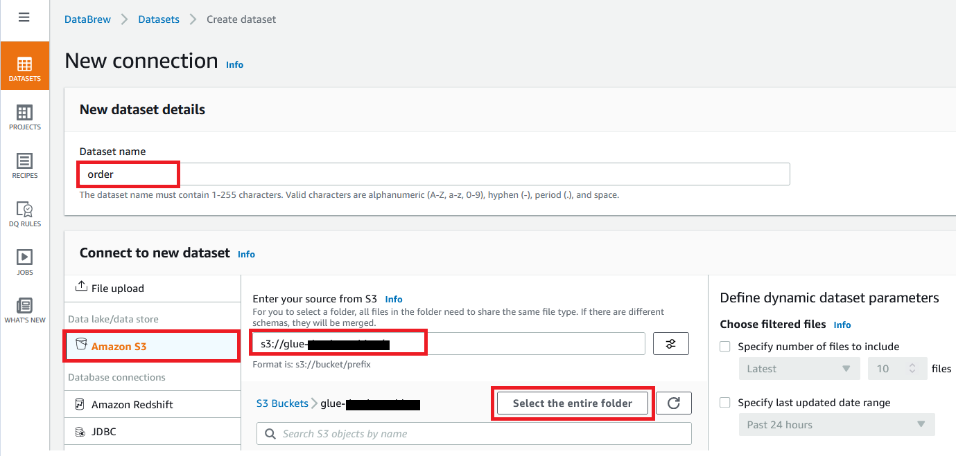
What to consider when migrating data warehouse to Amazon Redshift

Post Syndicated from Lewis Tang original https://aws.amazon.com/blogs/big-data/what-to-consider-when-migrating-data-warehouse-to-amazon-redshift/

Customers are migrating data warehouses to Amazon Redshift because it’s fast, scalable, and cost-effective. However, data warehouse migration projects can be complex and challenging. In this post, I help you understand the common drivers of data warehouse migration, migration strategies, and what tools and services are available to assist with your migration project.

Let’s first discuss the big data landscape, the meaning of a modern data architecture, and what you need to consider for your data warehouse migration project when building a modern data architecture.

Business opportunities

Data is changing the way we work, live, and play. All of this behavior change and the movement to the cloud has resulted in a data explosion over the past 20 years. The proliferation of Internet of Things and smart phones have accelerated the amount of the data that is generated every day. Business models have shifted, and so have the needs of the people running these businesses. We have moved from talking about terabytes of data just a few years ago to now petabytes and exabytes of data. By putting data to work efficiently and building deep business insights from the data collected, businesses in different industries and of various sizes can achieve a wide range of business outcomes. These can be broadly categorized into the following core business outcomes:

  • Improving operational efficiency – By making sense of the data collected from various operational processes, businesses can improve customer experience, increase production efficiency, and increase sales and marketing agility
  • Making more informed decisions – Through developing more meaningful insights by bringing together full picture of data across an organization, businesses can make more informed decisions
  • Accelerating innovation – Combining internal and external data sources enable a variety of AI and machine learning (ML) use cases that help businesses automate processes and unlock business opportunities that were either impossible to do or too difficult to do before

Business challenges

Exponential data growth has also presented business challenges.

First of all, businesses need to access all data across the organization, and data may be distributed in silos. It comes from a variety of sources, in a wide range of data types and in large volume and velocity. Some data may be stored as structured data in relational databases. Other data may be stored as semi-structured data in object stores, such as media files and the clickstream data that is constantly streaming from mobile devices.

Secondly, to build insights from data, businesses need to dive deep into the data by conducting analytics. These analytics activities generally involve dozens and hundreds of data analysts who need to access the system simultaneously. Having a performant system that is scalable to meet the query demand is often a challenge. It gets more complex when businesses need to share the analyzed data with their customers.

Last but not least, businesses need a cost-effective solution to address data silos, performance, scalability, security, and compliance challenges. Being able to visualize and predict cost is necessary for a business to measure the cost-effectiveness of its solution.

To solve these challenges, businesses need a future proof modern data architecture and a robust, efficient analytics system.

Modern data architecture

A modern data architecture enables organizations to store any amount of data in open formats, break down disconnected data silos, empower users to run analytics or ML using their preferred tool or technique, and manage who has access to specific pieces of data with the proper security and data governance controls.

The AWS data lake architecture is a modern data architecture that enables you to store data in a data lake and use a ring of purpose-built data services around the lake, as shown in the following figure. This allows you to make decisions with speed and agility, at scale, and cost-effectively. For more details, refer to Modern Data Architecture on AWS.

Modern data warehouse

Amazon Redshift is a fully managed, scalable, modern data warehouse that accelerates time to insights with fast, easy, and secure analytics at scale. With Amazon Redshift, you can analyze all your data and get performance at any scale with low and predictable costs.

Amazon Redshift offers the following benefits:

  • Analyze all your data – With Amazon Redshift, you can easily analyze all your data across your data warehouse and data lake with consistent security and governance policies. We call this the modern data architecture. With Amazon Redshift Spectrum, you can query data in your data lake with no need for loading or other data preparation. And with data lake export, you can save the results of an Amazon Redshift query back into the lake. This means you can take advantage of real-time analytics and ML/AI use cases without re-architecture, because Amazon Redshift is fully integrated with your data lake. With new capabilities like data sharing, you can easily share data across Amazon Redshift clusters both internally and externally, so everyone has a live and consistent view of the data. Amazon Redshift ML makes it easy to do more with your data—you can create, train, and deploy ML models using familiar SQL commands directly in Amazon Redshift data warehouses.
  • Fast performance at any scale – Amazon Redshift is a self-tuning and self-learning system that allows you to get the best performance for your workloads without the undifferentiated heavy lifting of tuning your data warehouse with tasks such as defining sort keys and distribution keys, and new capabilities like materialized views, auto-refresh, and auto-query rewrite. Amazon Redshift scales to deliver consistently fast results from gigabytes to petabytes of data, and from a few users to thousands. As your user base scales to thousands of concurrent users, the concurrency scaling capability automatically deploys the necessary compute resources to manage the additional load. Amazon Redshift RA3 instances with managed storage separate compute and storage, so you can scale each independently and only pay for the storage you need. AQUA (Advanced Query Accelerator) for Amazon Redshift is a new distributed and hardware-accelerated cache that automatically boosts certain types of queries.

  • Easy analytics for everyone – Amazon Redshift is a fully managed data warehouse that abstracts away the burden of detailed infrastructure management or performance optimization. You can focus on getting to insights, rather than performing maintenance tasks like provisioning infrastructure, creating backups, setting up the layout of data, and other tasks. You can operate data in open formats, use familiar SQL commands, and take advantage of query visualizations available through the new Query Editor v2. You can also access data from any application through a secure data API without configuring software drivers, managing database connections. Amazon Redshift is compatible with business intelligence (BI) tools, opening up the power and integration of Amazon Redshift to business users who operate from within the BI tool.

A modern data architecture with a data lake architecture and modern data warehouse with Amazon Redshift helps businesses in all different sizes address big data challenges, make sense of a large amount of data, and drive business outcomes. You can start the journey of building a modern data architecture by migrating your data warehouse to Amazon Redshift.

Migration considerations

Data warehouse migration presents a challenge in terms of project complexity and poses a risk in terms of resources, time, and cost. To reduce the complexity of data warehouse migration, it’s essential to choose a right migration strategy based on your existing data warehouse landscape and the amount of transformation required to migrate to Amazon Redshift. The following are the key factors that can influence your migration strategy decision:

  • Size – The total size of the source data warehouse to be migrated is determined by the objects, tables, and databases that are included in the migration. A good understanding of the data sources and data domains required for moving to Amazon Redshift leads to an optimal sizing of the migration project.
  • Data transfer – Data warehouse migration involves data transfer between the source data warehouse servers and AWS. You can either transfer data over a network interconnection between the source location and AWS such as AWS Direct Connect or transfer data offline via the tools or services such as the AWS Snow Family.
  • Data change rate – How often do data updates or changes occur in your data warehouse? Your existing data warehouse data change rate determines the update intervals required to keep the source data warehouse and the target Amazon Redshift in sync. A source data warehouse with a high data change rate requires the service switching from the source to Amazon Redshift to complete within an update interval, which leads to a shorter migration cutover window.
  • Data transformation – Moving your existing data warehouse to Amazon Redshift is a heterogenous migration involving data transformation such as data mapping and schema change. The complexity of data transformation determines the processing time required for an iteration of migration.
  • Migration and ETL tools – The selection of migration and extract, transform, and load (ETL) tools can impact the migration project. For example, the efforts required for deployment and setup of these tools can vary. We look closer at AWS tools and services shortly.

After you have factored in all these considerations, you can pick a migration strategy option for your Amazon Redshift migration project.

Migration strategies

You can choose from three migration strategies: one-step migration, two-step migration, or wave-based migration.

One-step migration is a good option for databases that don’t require continuous operation such as continuous replication to keep ongoing data changes in sync between the source and destination. You can extract existing databases as comma separated value (CSV) files, or columnar format like Parquet, then use AWS Snow Family services such as AWS Snowball to deliver datasets to Amazon Simple Storage Service (Amazon S3) for loading into Amazon Redshift. You then test the destination Amazon Redshift database for data consistency with the source. After all validations have passed, the database is switched over to AWS.

Two-step migration is commonly used for databases of any size that require continuous operation, such as the continuous replication. During the migration, the source databases have ongoing data changes, and continuous replication keeps data changes in sync between the source and Amazon Redshift. The breakdown of the two-step migration strategy is as follows:

  • Initial data migration – The data is extracted from the source database, preferably during non-peak usage to minimize the impact. The data is then migrated to Amazon Redshift by following the one-step migration approach described previously.
  • Changed data migration – Data that changed in the source database after the initial data migration is propagated to the destination before switchover. This step synchronizes the source and destination databases. After all the changed data is migrated, you can validate the data in the destination database and perform necessary tests. If all tests are passed, you then switch over to the Amazon Redshift data warehouse.

Wave-based migration is suitable for large-scale data warehouse migration projects. The principle of wave-based migration is taking precautions to divide a complex migration project into multiple logical and systematic waves. This strategy can significantly reduce the complexity and risk. You start from a workload that covers a good number of data sources and subject areas with medium complexity, then add more data sources and subject areas in each subsequent wave. With this strategy, you run both the source data warehouse and Amazon Redshift production environments in parallel for a certain amount of time before you can fully retire the source data warehouse. See Develop an application migration methodology to modernize your data warehouse with Amazon Redshift for details on how to identify and group data sources and analytics applications to migrate from the source data warehouse to Amazon Redshift using the wave-based migration approach.

To guide your migration strategy decision, refer to the following table to map the consideration factors with a preferred migration strategy.

. One-Step Migration Two-Step Migration Wave-Based Migration
The number of subject areas in migration scope Small Medium to Large Medium to Large
Data transfer volume Small to Large Small to Large Small to Large
Data change rate during migration None Minimal to Frequent Minimal to Frequent
Data transformation complexity Any Any Any
Migration change window for switching from source to target Hours Seconds Seconds
Migration project duration Weeks Weeks to Months Months

Migration process

In this section, we review the three high-level steps of the migration process. The two-step migration strategy and wave-based migration strategy involve all three migration steps. However, the wave-based migration strategy includes a number of iterations. Because only databases that don’t require continuous operations are good fits for one-step migration, only Steps 1 and 2 in the migration process are required.

Step 1: Convert schema and subject area

In this step, you make the source data warehouse schema compatible with the Amazon Redshift schema by converting the source data warehouse schema using schema conversion tools such as AWS Schema Conversion Tool (AWS SCT) and the other tools from AWS partners. In some situations, you may also be required to use custom code to conduct complex schema conversions. We dive deeper into AWS SCT and migration best practices in a later section.

Step 2: Initial data extraction and load

In this step, you complete the initial data extraction and load the source data into Amazon Redshift for the first time. You can use AWS SCT data extractors to extract data from the source data warehouse and load data to Amazon S3 if your data size and data transfer requirements allow you to transfer data over the interconnected network. Alternatively, if there are limitations such as network capacity limit, you can load data to Snowball and from there data gets loaded to Amazon S3. When the data in the source data warehouse is available on Amazon S3, it’s loaded to Amazon Redshift. In situations when the source data warehouse native tools do a better data unload and load job than AWS SCT data extractors, you may choose to use the native tools to complete this step.

Step 3: Delta and incremental load

In this step, you use AWS SCT and sometimes source data warehouse native tools to capture and load delta or incremental changes from sources to Amazon Redshift. This is often referred to change data capture (CDC). CDC is a process that captures changes made in a database, and ensures that those changes are replicated to a destination such as a data warehouse.

You should now have enough information to start developing a migration plan for your data warehouse. In the following section, I dive deeper into the AWS services that can help you migrate your data warehouse to Amazon Redshift, and the best practices of using these services to accelerate a successful delivery of your data warehouse migration project.

Data warehouse migration services

Data warehouse migration involves a set of services and tools to support the migration process. You begin with creating a database migration assessment report and then converting the source data schema to be compatible with Amazon Redshift by using AWS SCT. To move data, you can use the AWS SCT data extraction tool, which has integration with AWS Data Migration Service (AWS DMS) to create and manage AWS DMS tasks and orchestrate data migration.

To transfer source data over the interconnected network between the source and AWS, you can use AWS Storage Gateway, Amazon Kinesis Data Firehose, Direct Connect, AWS Transfer Family services, Amazon S3 Transfer Acceleration, and AWS DataSync. For data warehouse migration involving a large volume of data, or if there are constraints with the interconnected network capacity, you can transfer data using the AWS Snow Family of services. With this approach, you can copy the data to the device, send it back to AWS, and have the data copied to Amazon Redshift via Amazon S3.

AWS SCT is an essential service to accelerate your data warehouse migration to Amazon Redshift. Let’s dive deeper into it.

Migrating using AWS SCT

AWS SCT automates much of the process of converting your data warehouse schema to an Amazon Redshift database schema. Because the source and target database engines can have many different features and capabilities, AWS SCT attempts to create an equivalent schema in your target database wherever possible. If no direct conversion is possible, AWS SCT creates a database migration assessment report to help you convert your schema. The database migration assessment report provides important information about the conversion of the schema from your source database to your target database. The report summarizes all the schema conversion tasks and details the action items for schema objects that can’t be converted to the DB engine of your target database. The report also includes estimates of the amount of effort that it will take to write the equivalent code in your target database that can’t be converted automatically.

Storage optimization is the heart of a data warehouse conversion. When using your Amazon Redshift database as a source and a test Amazon Redshift database as the target, AWS SCT recommends sort keys and distribution keys to optimize your database.

With AWS SCT, you can convert the following data warehouse schemas to Amazon Redshift:

  • Amazon Redshift
  • Azure Synapse Analytics (version 10)
  • Greenplum Database (version 4.3 and later)
  • Microsoft SQL Server (version 2008 and later)
  • Netezza (version 7.0.3 and later)
  • Oracle (version 10.2 and later)
  • Snowflake (version 3)
  • Teradata (version 13 and later)
  • Vertica (version 7.2 and later)

At AWS, we continue to release new features and enhancements to improve our product. For the latest supported conversions, visit the AWS SCT User Guide.

Migrating data using AWS SCT data extraction tool

You can use an AWS SCT data extraction tool to extract data from your on-premises data warehouse and migrate it to Amazon Redshift. The agent extracts your data and uploads the data to either Amazon S3 or, for large-scale migrations, an AWS Snowball Family service. You can then use AWS SCT to copy the data to Amazon Redshift. Amazon S3 is a storage and retrieval service. To store an object in Amazon S3, you upload the file you want to store to an S3 bucket. When you upload a file, you can set permissions on the object and also on any metadata.

In large-scale migrations involving data upload to a AWS Snowball Family service, you can use wizard-based workflows in AWS SCT to automate the process in which the data extraction tool orchestrates AWS DMS to perform the actual migration.

Considerations for Amazon Redshift migration tools

To improve and accelerate data warehouse migration to Amazon Redshift, consider the following tips and best practices. Tthis list is not exhaustive. Make sure you have a good understanding of your data warehouse profile and determine which best practices you can use for your migration project.

  • Use AWS SCT to create a migration assessment report and scope migration effort.
  • Automate migration with AWS SCT where possible. The experience from our customers shows that AWS SCT can automatically create the majority of DDL and SQL scripts.
  • When automated schema conversion is not possible, use custom scripting for the code conversion.
  • Install AWS SCT data extractor agents as close as possible to the data source to improve data migration performance and reliability.
  • To improve data migration performance, properly size your Amazon Elastic Compute Cloud (Amazon EC2) instance and its equivalent virtual machines that the data extractor agents are installed on.
  • Configure multiple data extractor agents to run multiple tasks in parallel to improve data migration performance by maximizing the usage of the allocated network bandwidth.
  • Adjust AWS SCT memory configuration to improve schema conversion performance.
  • Use Amazon S3 to store the large objects such as images, PDFs, and other binary data from your existing data warehouse.
  • To migrate large tables, use virtual partitioning and create sub-tasks to improve data migration performance.
  • Understand the use cases of AWS services such as Direct Connect, the AWS Transfer Family, and the AWS Snow Family. Select the right service or tool to meet your data migration requirements.
  • Understand AWS service quotas and make informed migration design decisions.

Summary

Data is growing in volume and complexity faster than ever. However, only a fraction of this invaluable asset is available for analysis. Traditional on-premises data warehouses have rigid architectures that don’t scale for modern big data analytics use cases. These traditional data warehouses are expensive to set up and operate, and require large upfront investments in both software and hardware.

In this post, we discussed Amazon Redshift as a fully managed, scalable, modern data warehouse that can help you analyze all your data, and achieve performance at any scale with low and predictable cost. To migrate your data warehouse to Amazon Redshift, you need to consider a range of factors, such as the total size of the data warehouse, data change rate, and data transformation complexity, before picking a suitable migration strategy and process to reduce the complexity and cost of your data warehouse migration project. With AWS services such AWS SCT and AWS DMS, and by adopting the tips and the best practices of these services, you can automate migration tasks, scale migration, accelerate the delivery of your data warehouse migration project, and delight your customers.


About the Author

Lewis Tang is a Senior Solutions Architect at Amazon Web Services based in Sydney, Australia. Lewis provides partners guidance to a broad range of AWS services and help partners to accelerate AWS practice growth.