At Grab, we continuously enhance our systems to improve scalability, reliability and cost-efficiency. Recently, we undertook a project to split the read and write functionalities of one of our backend services into separate services. This was motivated by the need to independently scale these operations based on their distinct scalability requirements.
In this post, we will dive deep into how we migrated the stream processing (write) functionality to a new service with zero data loss and duplication. This was accomplished while handling a high volume of real-time traffic averaging 20,000 reads per second from 16 source Kafka streams writing to other output streams and several DynamoDB tables.
Migration challenges and strategy
Migrating the stream processing to the new service while ensuring zero data loss and duplication posed some interesting challenges, especially given the high volume of real-time data. We needed a strategy that would enable us to:
Migrate streams one by one gradually.
Validate the new service’s processing in production before fully switching over.
Perform the switchover with no downtime or data inconsistencies.
We considered various options for the switchover such as using feature flags via our unified config management and experimental rollout platform. However, these approaches had some limitations:
There could be some data loss or duplication during the deployment time when toggling the flags, which can be up to a few minutes.
There might be data inconsistencies as the flag value could be updated on the services (the existing and and the new one) at slightly different times.
Ultimately, we decided on a custom time-based switchover logic implemented in shared code between the two services leveraging our monorepo structure. In the following sections, we will walk you through the steps we took to achieve this seamless migration.
Step 1: Preparation
First, since both the existing and new services reside in our monorepo, we moved the stream processing code from the existing service to a shared /commons directory. This allowed both the old and new services to import and use the same code. We added logic in this commons package to selectively turn stream processing on or off based on the service processing them.
Next, we created temporary “sink” resources such as streams and DynamoDB tables for the new service to write the processed data. This allowed us to monitor and validate the new service’s behavior in production without impacting the main resources.
Figure 1. For a short period, both services consumed the incoming streams, but only the old service continued to write to the actual sink resources while the new service wrote to validation sink resources.
Step 2: Scheduling the switchover
In the shared /commons code, we added a map[string]time.Time to schedule the switchover for each stream.
When a stream is added to this map, it means it is scheduled for switchover at the specified time. This logic is shared between both services, so the switchover happens simultaneously. The new service starts writing to the main resources while the old service stops, with no overlap or gap.
Step 3: Deployment and monitoring
To perform the switchover, we:
Updated the switchover times for the streams.
Deployed both services with enough buffer time before the scheduled switch.
Closely monitored the process by creating dedicated monitors for the migration process using our observability tools.
Figure 2. This timeseries graph shows the stream received at the old and the new service (dotted line), facilitating real time monitoring of the stream processing volume across both services during the validation period.
The old service continued consuming the streams for a short monitoring period post-switchover, but without writing anywhere, ensuring no loss or duplication at the output sink resources. Then, the stream consumption was removed from the old service altogether, completing the entire migration process.
Results and learnings
Using this time-based approach, we were able to seamlessly migrate the high-volume stream processing to the new service with:
Zero data loss or duplication.
No downtime or production issues.
The whole migration, including the gradual stream-by-stream switchover, was completed in about three weeks.
One learning was that such custom time-based logic, while effective for our use case, has limitations. If a rollback was needed for any of the two services for some unexpected reasons, some data inconsistency would be unavoidable. Generally, such time-based logic should be used with caution as it can lead to unexpected scenarios if the systems fall out of sync. We went ahead with this approach as it was a temporary measure and we had thoroughly tested it before carrying out the switchover.
Join us
Grab is the leading superapp platform in Southeast Asia, providing everyday services that matter to consumers. More than just a ride-hailing and food delivery app, Grab offers a wide range of on-demand services in the region, including mobility, food, package and grocery delivery services, mobile payments, and financial services across 700 cities in eight countries.
Powered by technology and driven by heart, our mission is to drive Southeast Asia forward by creating economic empowerment for everyone. If this mission speaks to you, join our team today!
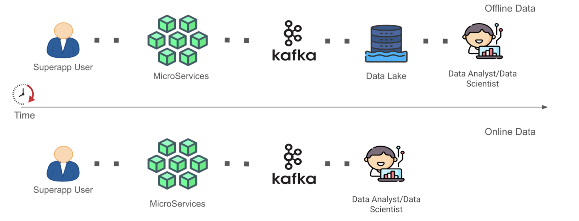
In this digital age, companies collect multitudes of data that enable the tracking of business metrics and performance. Over the years, data analytics tools for data storage and processing have evolved from the days of Excel sheets and macros to more advanced Map Reduce model tools like Spark, Hadoop, and Hive. This evolution has allowed companies, including Grab, to perform modern analytics on the data ingested into the Data Lake, empowering them to make better data-driven business decisions. This form of data will be referenced within this document as “Offline Data”.
With innovations in stream processing technology like Spark and Flink, there is now more interest in unlocking value from streaming data. This form of continuously-generated data in high volume will be referenced within this document as “Online Data”. In the context of Grab, the streaming data is usually materialised as Kafka topics (“Kafka Stream”) as the result of stream processing in its framework. This data is largely unexplored until they are eventually sunk into the Data Lake as Offline Data, part of the data journey (see Figure 1 below). This induces some data latency before the data can be used by data analysts to inform decisions.
Figure 1. Simplified data journey for Offline Data vs. Online Data, from data generation to data analysis.
As seen in Figure 1 above, the Time to Value (“TTV”) of Online Data is shorter as compared to that of Offline Data in a simplified data journey from data generation to data analysis where complexities of data cleaning and transformation have been removed. This is because the role of the data analyst or data scientist (“Data End User”) has been enabled forward to the Kafka stage for Online Data instead of the Data Lake stage for Offline Data. We recognise that allowing earlier data exploration on Online Data allows Data End Users to build context around the data inputs they are using in an earlier stage. This can help them process Offline Data more meaningfully in subsequent stages. We are interested in opening up the possibility for Data End Users to at least explore the Online Data before they architect a full solution to clean and/or process the data directly or more efficiently post-ingestion into the Data Lake. After their data exploration, the users would have more information to decide whether to spin up a stream processing pipeline for Online Data, or to continue processing Offline Data with their current solution, but with a more refined understanding and logic strategy against their source data inputs. However, of course, in this blog, we acknowledge that not all analysis on Online Data could be done in this manner.
Problem statement
Online Data is underutilised within Grab mainly because of, among other reasons, difficulty in performing data exploration on data that is not yet properly stored in the Data Lake.
For the purpose of this blog post, we will focus only on the problem of exploration of Online Data because this problem is the precursor to allowing us to fully democratise such data.
The problem of data exploration manifests itself when Data End Users need to find the proper data inputs to base and develop their data models. These users would then often need to parse through a multitude of documentation and connect with multiple upstream data producers, to know the range of data signals that are currently available and understand what each data signal is trying to measure.
Given the ephemeral nature of Online Data, this implies that the lack of correct tool adoption to seamlessly perform quick tests with application logic on Online Data disincentivises the Data End Users to work on these Online Data. Testing such logic on Offline Data is generally much easier since iteration testing on the exact same dataset is possible.
This difficulty in performing data exploration including ad hoc queries on Online Data has therefore made development of stream processing applications hard for Data End Users, creating headwinds in Grab’s aim to evolve from making data-driven business decisions to also making data-driven operation decisions. Doing both would allow Grab to react much quicker to abrupt changes in its business landscape.
Adoption of Zeppelin notebook environment
To address the difficulty in performing data exploration on Online Data, we have adopted Apache Zeppelin, a web-based notebook that enables data-drive, interactive data analytics with the support of multiple interpreters to work with various data processing backends e.g. Spark, Flink. The full solution of the adopted Zeppelin notebook environment is enabled seamlessly within our internal data-streaming platform, through its control plane. If you are interested, you may check out our previous blog post titled An elegant platform for more details on the abovementioned streaming platform and its control plane.
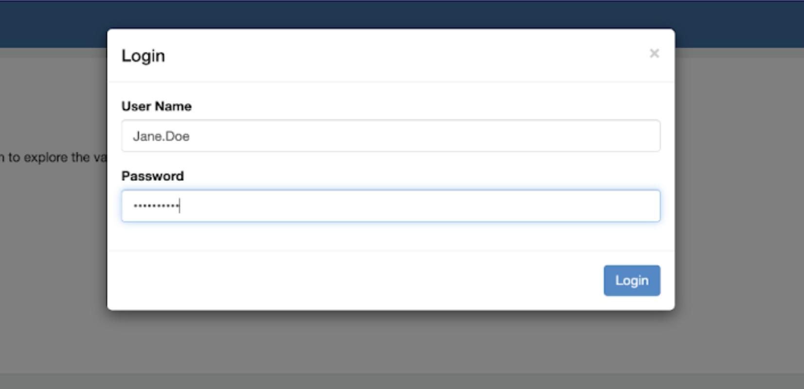
Figure 2. Zeppelin login page via web-based notebook environment.
As seen from Figure 2 above, after successful creation of the Zeppelin cluster, users can log in with their generated credentials delivered to them via the integrated instant messenger, and start using the notebook environment.
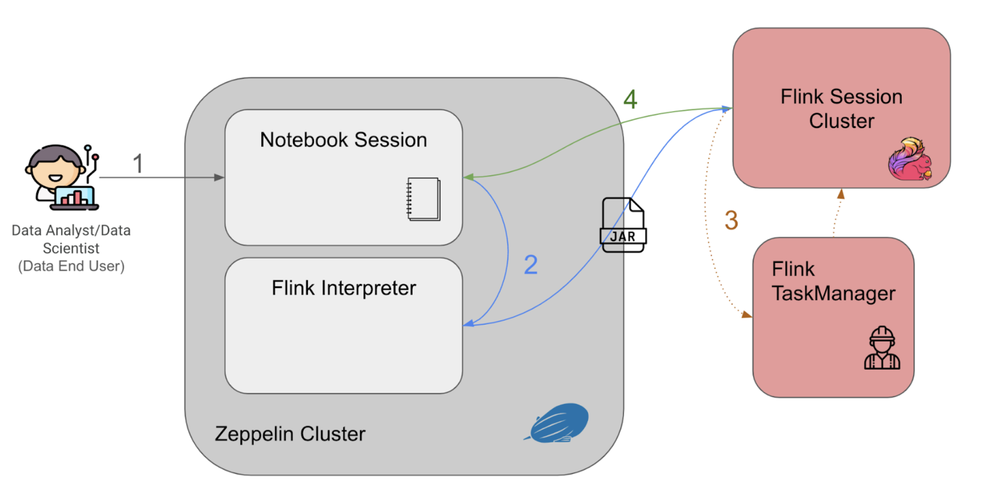
Figure 3. Zeppelin programme flow in the notebook environment.
Figure 3 above explains the Zeppelin notebook programme flow as follows:
The users enter their queries into the notebook session and run querying statements interactively with the established web-based notebook session.
The queries are passed to the Flink interpreter within the cluster to generate the Flink job as a Jar file, to be then submitted to a Flink session cluster.
When the Flink session cluster job manager receives the job, it would spin up the corresponding Flink task managers (workers) to run the application and retrieve the results.
The query results would then be piped back to the notebook session, to be displayed back to the user on the notebook session.
Data query and visualisation
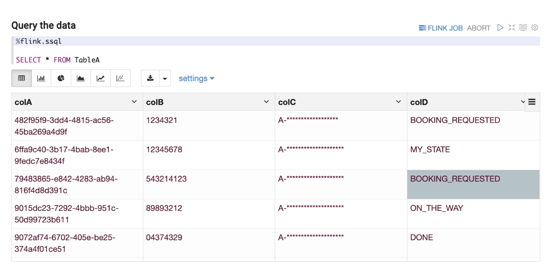
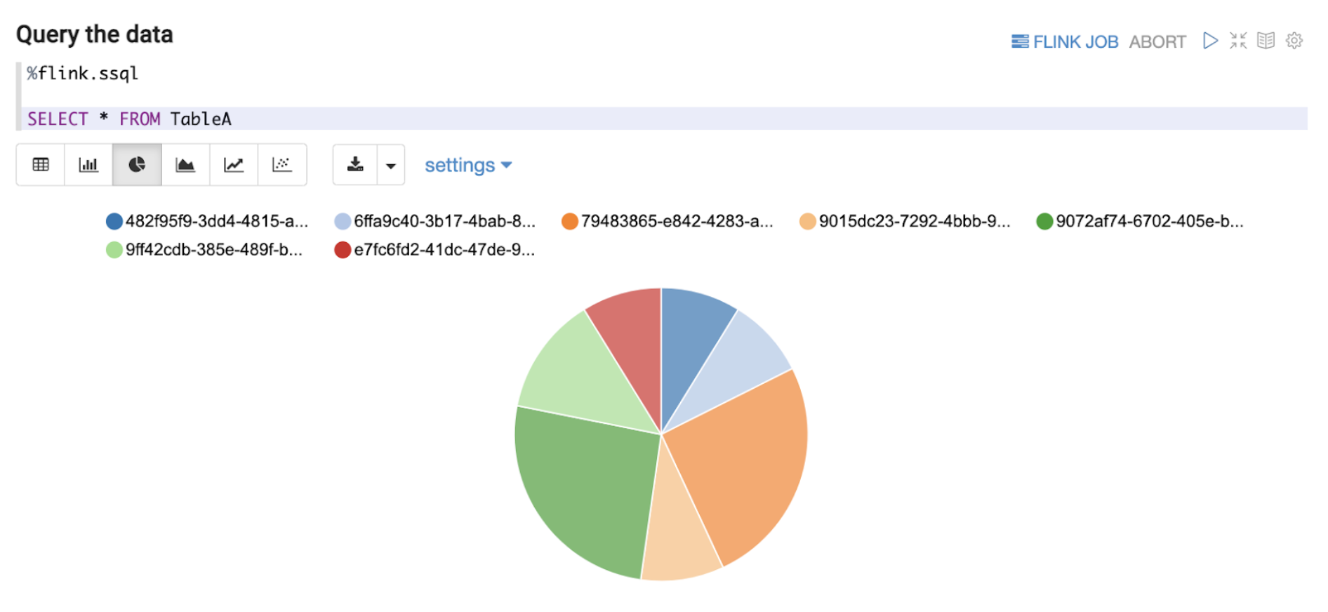
Figure 4. Example of simple select query of data on Kafka. Note: All variable names, schema, values, and other details used in this article are only created for use as examples.
Flink has a planned roadmap to create a unified streaming language for both stream processing and data analytics. In line with the roadmap, we have based our Zeppelin solution on supporting Structured Query Language (“SQL”) as the query language of choice as seen in Figure 4 above. Data End Users can now write queries in SQL, which is a language that they are comfortable with, and perform adequate data exploration.
As discussed in this section, data exploration on streaming data at the Kafka stage by adopting the right tool enables Data End Users to seamlessly have visibility to quickly understand the current schema of a Kafka topic (explained more in the next section. This kind of data exploration also enables Data End Users to understand the type of data the Kafka topic represents, such as the ability to determine if a country code data field is in alpha-2 or alpha-3 format while the data is still part of streaming data. This might seem inconsequential and immediately identifiable even in Offline Data, but by enabling data exploration at an earlier stage in the data journey for Online Data, Data End Users have the opportunity to react much more quickly. For example, a change of expected country code format from the data producer would usually lead to errors in the downstream joins or other stream processing pipelines due to incompatible parsing or filtering of the modified country codes. Instead of waiting for the data to be ingested to Offline Data, users can investigate the issue with Online Data retrieved from Kafka.
Figure 5. Simple visualisation of queried data on Zeppelin’s notebook environment. Note: All variable names, schema, values, and other details used in this article are only created for use as examples.
Besides query features, Zeppelin notebook provides simple visualisation and analytics of the off-the-shelf data as presented above in Figure 5. Furthermore, users are now able to perform interactive ad hoc queries on Online Data. These queries will eventually become much more advanced and/or effective SQL queries to be deployed as a streaming pipeline later on in the data journey. This reduces the inertia in setting up a separate development environment or learning other programming languages like Java or Scala during the development of streaming pipelines. With Zeppelin’s notebook environment, our Data End Users are more empowered to quickly derive value from Online Data.
Need for a more dynamic table schema derivation process
For the Data End Users performing data exploration on Online Data, we see a need for these users to derive the Data Definition Language (“DDL”) associated with a Kafka stream at an earlier stage of the data journey. Within Grab, even though Kafka streams are transmitted in Protobuf format and are thus structured, both the schema and the corresponding DDL changes are added over time as new fields. Typically, the data producer (service owners) and the data engineers responsible for the data ingestion pipeline coordinate to perform such updates. Since the Data End Users are not involved in such schema update processes nor do they directly interact with the data producers, many of them find the discovery of changes in the current Kafka stream schema an issue. Granted that this is an issue our metadata platform is actively solving using Datahub, we hope to also solve the challenge by being able to derive the DDL more dynamically within the tooling, for data exploration on Online Data to reduce friction.
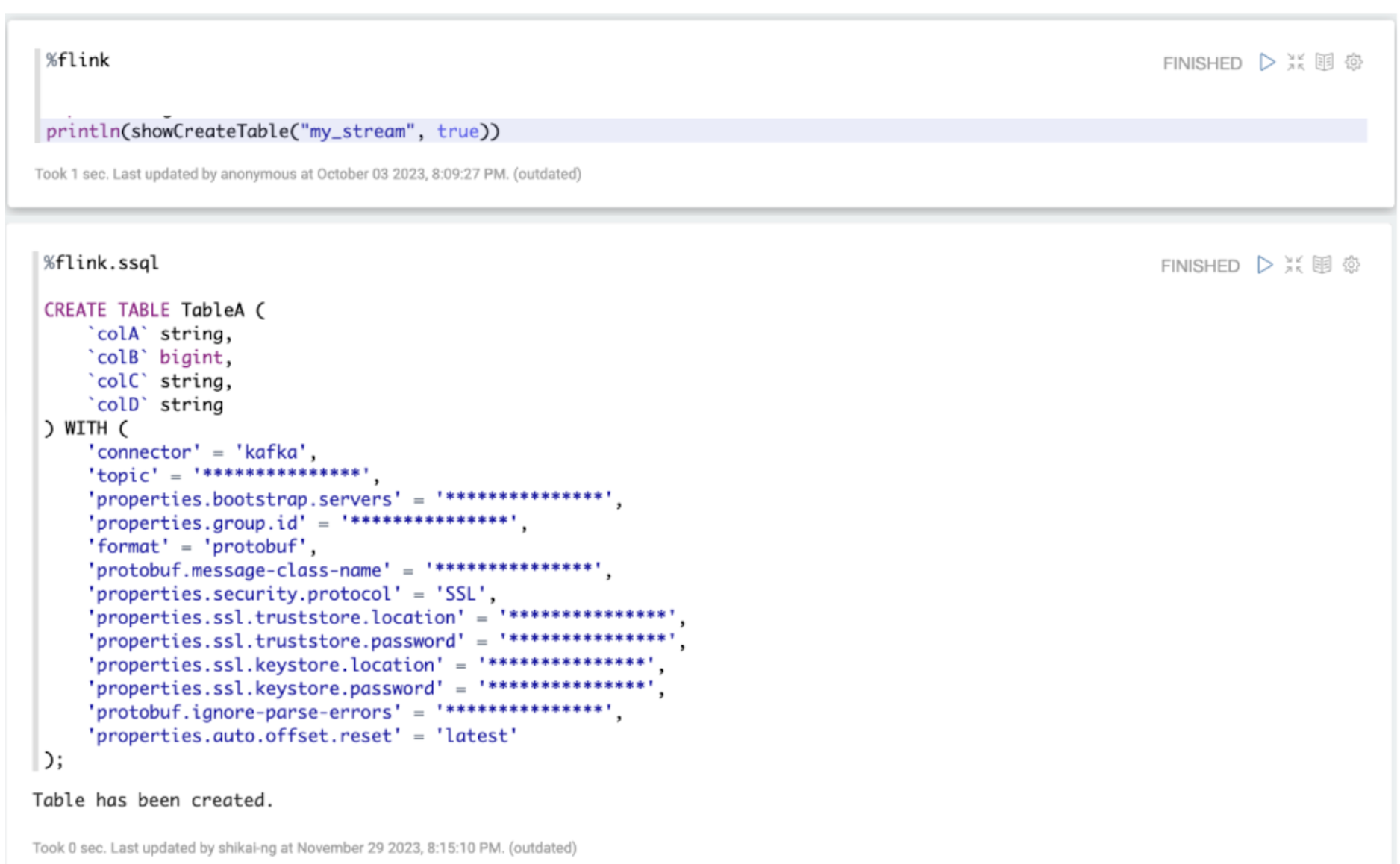
Figure 6. Common functions to derive DDL of a Kafka Stream in SQL. Note: All variable names, schema, values, and other details used in this article are only created for use as examples.
As seen from Figure 6 above, we have an integrated tooling for Data End Users to derive the DDL associated with a Kafka stream using SQL language. A Kafka stream in Grab’s context is a logical concept describing a Kafka topic, associating it with its metadata like Kafka bootstrap servers and associated Java class created by Protoc. This tool maps the Protobuf schema definition of a Kafka stream to a DDL, allowing it to be expressed and used in SQL language. This reduces the manual effort involved in creating these table definitions from scratch based on the associated Protobuf schema. Users can now derive the DDL associated with a Kafka stream more easily.
Mitigating risks arising from data exploration on Online Data – data access authorisation/audit
While we rethink stream processing and are open to options that enable data exploration on Online Data as mentioned above, we realised that new security requirements related to data access authorisation and maintaining proper audit trail have emerged. Even with Personally Identifiable Information (PII) obfuscation enforcement by our streaming pipeline, it means we need to implement stricter guardrails in place along with audit trails to ensure users only have access to what they are allowed to, and this access can be removed in a break-glass scenario. If you are interested, you may check out our previous blog post titled PII masking for privacy-grade machine learning for more details about how we enforce PII masking on machine learning data streaming pipelines.
To enable data access authorisation, we utilised Strimzi, the operator of running Kafka on Kubernetes. We integrated Strimzi’s Open Policy Agent (OPA) with Kafka to define policies that authorise specific read-only user access to specific Kafka Topics. The identification of users is done via mutualTLS (mTLS) connection with our Kafka clusters, where their user details are part of the SSL certificate details used for authentication.
With these tools in place, each user’s request to explore Online Data would be properly logged, and each data access can be controlled by an OPA policy managed by a central team.
If you are interested, you may check out our previous post Zero trust with Kafka where we discussed our efforts to continue strengthening the security of our data-streaming platform.
Impact
With the proliferation of our data-streaming platform, we expect to see improvements in the way our data becomes gradually democratised. We have already been receiving use cases from the Data End Users who are interested in validating a chain of events on Online Data, i.e. retrieving information of all events associated with a particular booking, which is not currently something that can be done easily.
More importantly, the tools in place for data exploration on Online Data form the foundation required for us to embark on our next step of the stream processing journey. This foundation makes the development and validation of the stream processing logic much quicker. This occurs when ad hoc queries in a notebook environment are possible, removing the need for local developer environment setups and the need to go through the whole pipeline deployment process for eventual validation of the developed logic. We believe that this would prove to reduce our lead time in creating stream processing pipelines significantly.
What’s next?
Our next step is to rethink further how our stream processing pipelines are defined and start to provision SQL as the unified streaming language of our pipelines. This helps facilitate better discussion between upstream data producers, data engineers, and Data End Users, since SQL is the common language among these stakeholders.
We will also explore handling schema discovery in a more controlled manner by utilising a Hive catalogue to store our Kafka table definitions. This removes the need for users to retrieve and run the table DDL statement for every session, making the data exploration experience even more seamless.
Grab is the leading superapp platform in Southeast Asia, providing everyday services that matter to consumers. More than just a ride-hailing and food delivery app, Grab offers a wide range of on-demand services in the region, including mobility, food, package and grocery delivery services, mobile payments, and financial services across 428 cities in eight countries.
Powered by technology and driven by heart, our mission is to drive Southeast Asia forward by creating economic empowerment for everyone. If this mission speaks to you, join our team today!
Coban – Grab’s real-time data streaming platform – has been operating Kafka on Kubernetes with Strimzi in
production for about two years. In a previous article (Zero trust with Kafka), we explained how we leveraged Strimzi to enhance the security of our data streaming offering.
In this article, we are going to describe how we improved the fault tolerance of our initial design, to the point where we no longer need to intervene if a Kafka broker is unexpectedly terminated.
To make our operations easier and limit the blast radius of any incidents, we deploy exactly one Kafka cluster for each EKS cluster. We also give a full worker node to each Kafka broker. In terms of storage, we initially relied on EC2 instances with non-volatile memory express (NVMe) instance store volumes for
maximal I/O performance. Also, each Kafka cluster is accessible beyond its own Virtual Private Cloud (VPC) via a VPC Endpoint Service.
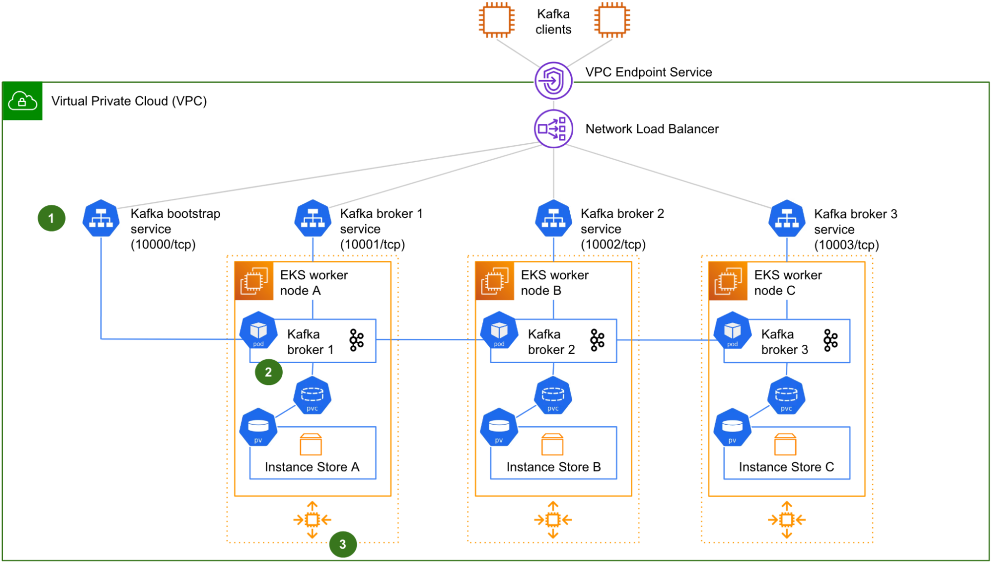
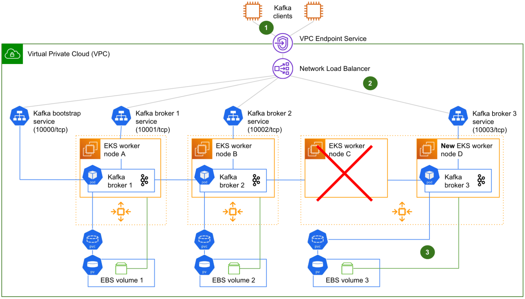
Fig. 1 Initial design of a 3-node Kafka cluster running on Kubernetes.
Fig. 1 shows a logical view of our initial design of a 3-node Kafka on Kubernetes cluster, as typically run by Coban. The Zookeeper and Cruise-Control components are not shown for clarity.
There are four Kubernetes services (1): one for the initial connection – referred to as “bootstrap” – that redirects incoming traffic to any Kafka pods, plus one for each Kafka pod, for the clients to target each Kafka broker individually (a requirement to produce or consume from/to a partition that resides on any particular Kafka broker). Four different listeners on the Network Load Balancer (NLB) listening on four different TCP ports, enable the Kafka clients to target either the bootstrap
service or any particular Kafka broker they need to reach. This is very similar to what we previously described in Exposing a Kafka Cluster via a VPC Endpoint Service.
Each worker node hosts a single Kafka pod (2). The NVMe instance store volume is used to create a Kubernetes Persistent Volume (PV), attached to a pod via a Kubernetes Persistent Volume Claim (PVC).
Lastly, the worker nodes belong to Auto-Scaling Groups (ASG) (3), one by Availability Zone (AZ). Strimzi adds in node affinity to make sure that the brokers are evenly distributed across AZs. In this initial design, ASGs are not for auto-scaling though, because we want to keep the size of the cluster under control. We only use ASGs – with a fixed size – to facilitate manual scaling operation and to automatically replace the terminated worker nodes.
With this initial design, let us see what happens in case of such a worker node termination.
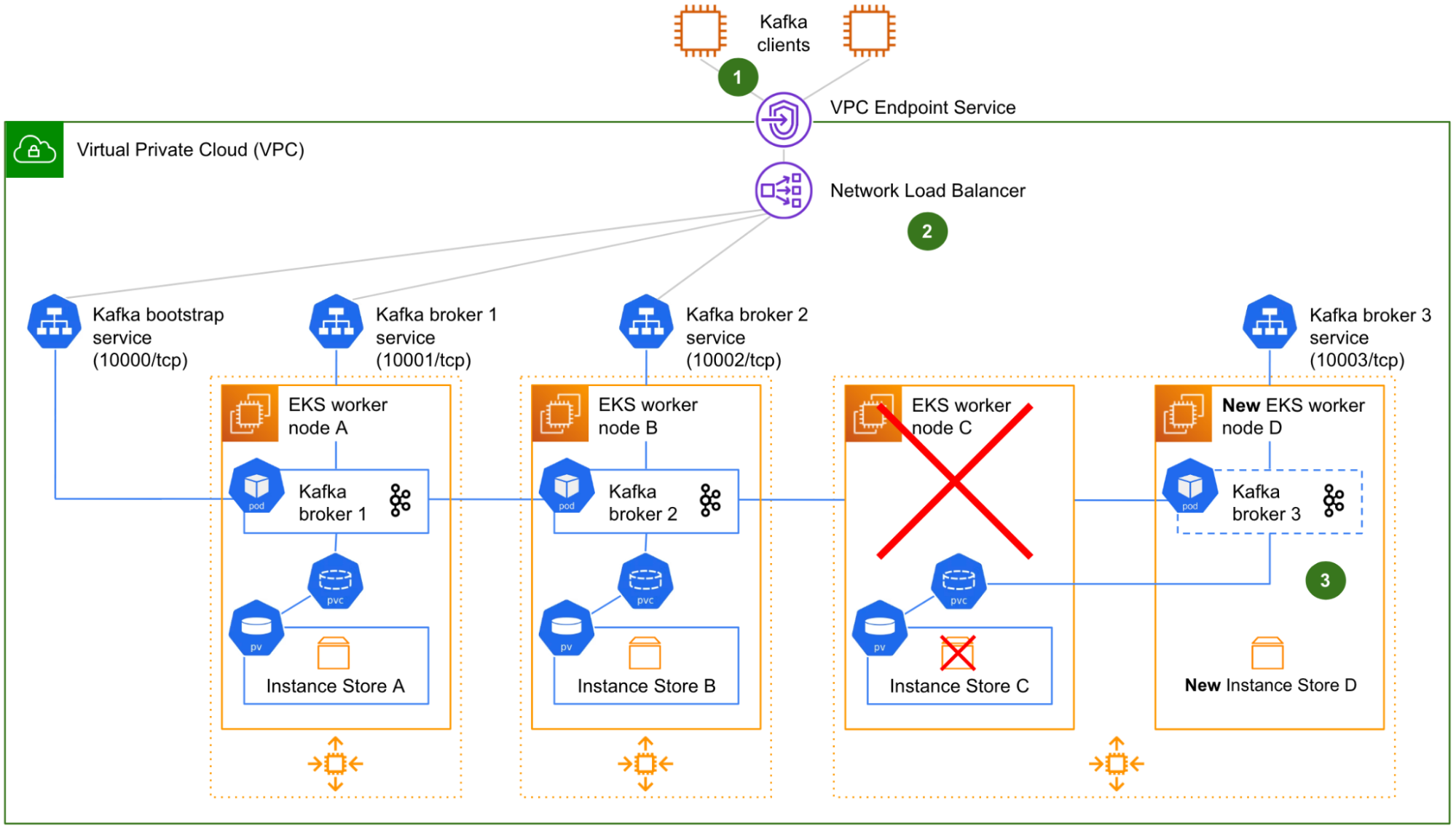
Fig. 2 Representation of a worker node termination. Node C is terminated and replaced by node D. However the Kafka broker 3 pod is unable to restart on node D.
Fig. 2 shows the worker node C being terminated along with its NVMe instance store volume C, and replaced (by the ASG) by a new worker node D and its new, empty NVMe instance store volume D. On start-up, the worker node D automatically joins the Kubernetes cluster. The Kafka broker 3 pod that was running on the faulty worker node C is scheduled to restart on the new worker node D.
Although the NVMe instance store volume C is terminated along with the worker node C, there is no data loss because all of our Kafka topics are configured with a minimum of three replicas. The data is poised to be copied over from the surviving Kafka brokers 1 and 2 back to Kafka broker 3, as soon as Kafka broker 3 is effectively restarted on the worker node D.
However, there are three fundamental issues with this initial design:
The Kafka clients that were in the middle of producing or consuming to/from the partition leaders of Kafka broker 3 are suddenly facing connection errors, because the broker was not gracefully demoted beforehand.
The target groups of the NLB for both the bootstrap connection and Kafka broker 3 still point to the worker node C. Therefore, the network communication from the NLB to Kafka broker 3 is broken. A manual reconfiguration of the target groups is required.
The PVC associating the Kafka broker 3 pod with its instance store PV is unable to automatically switch to the new NVMe instance store volume of the worker node D. Indeed, static provisioning is an intrinsic characteristic of Kubernetes local volumes. The PVC is still in Bound state, so Kubernetes does not take any action. However, the actual storage beneath the PV does not exist anymore. Without any storage, the Kafka broker 3 pod is unable to start.
At this stage, the Kafka cluster is running in a degraded state with only two out of three brokers, until a Coban engineer intervenes to reconfigure the target groups of the NLB and delete the zombie PVC (this, in turn, triggers its re-creation by Strimzi, this time using the new instance store PV).
In the next section, we will see how we have managed to address the three issues mentioned above to make this design fault-tolerant.
Solution
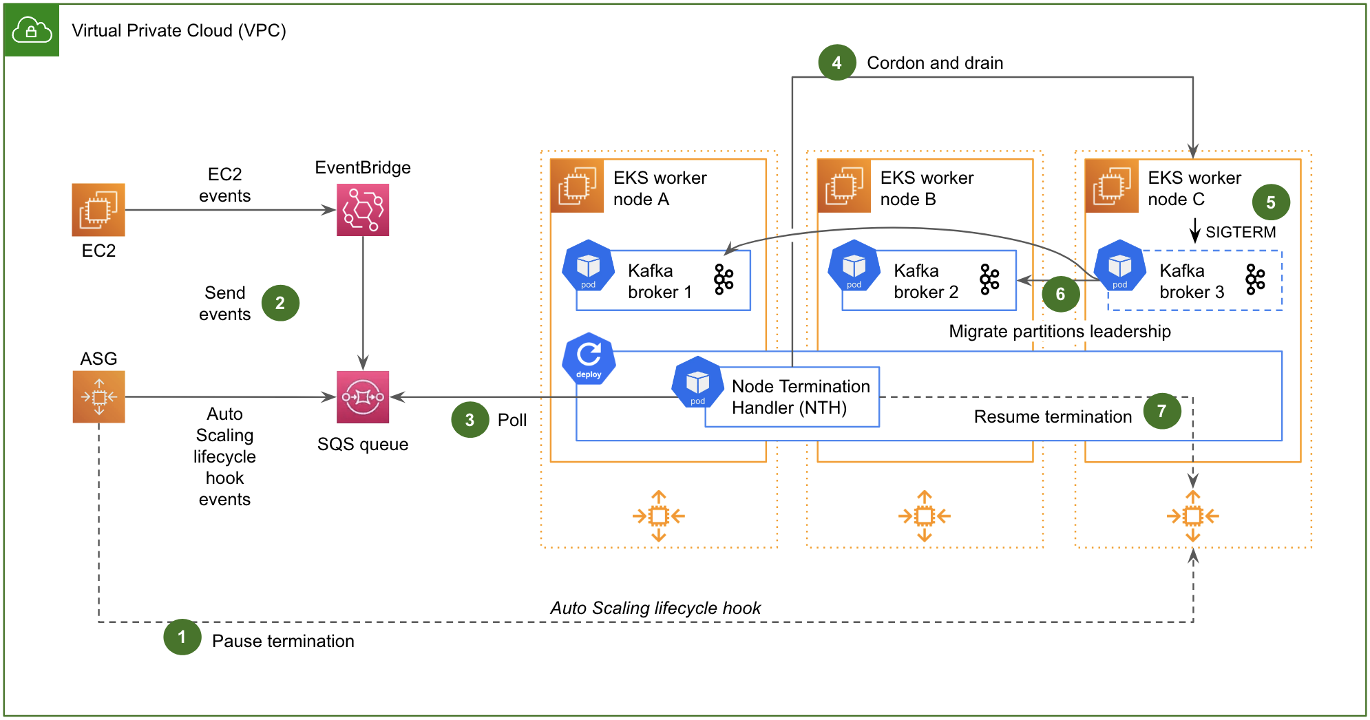
Graceful Kafka shutdown
To minimise the disruption for the Kafka clients, we leveraged the AWS Node Termination Handler (NTH). This component provided by AWS for Kubernetes environments is able to cordon and drain a worker node that is going to be terminated. This draining, in turn, triggers a graceful shutdown of the Kafka
process by sending a polite SIGTERM signal to all pods running on the worker node that is being drained (instead of the brutal SIGKILL of a normal termination).
The termination events of interest that are captured by the NTH are:
Scale-in operations by an ASG.
Manual termination of an instance.
AWS maintenance events, typically EC2 instances scheduled for upcoming retirement.
This suffices for most of the disruptions our clusters can face in normal times and our common maintenance operations, such as terminating a worker node to refresh it. Only sudden hardware failures (AWS issue events) would fall through the cracks and still trigger errors on the Kafka client side.
Fig. 3 Architecture of the NTH with the Queue Processor.
Fig. 3 shows the NTH with the Queue Processor in action, and how it reacts to a scale-in operation (typically triggered manually, during a maintenance operation):
As soon as the scale-in operation is triggered, an Auto Scaling lifecycle hook is invoked to pause the termination of the instance.
Simultaneously, an Auto Scaling lifecycle hook event is issued to an Amazon Simple Queue Service (SQS) queue. In Fig. 3, we have also materialised EC2 events (e.g. manual termination of an instance, AWS maintenance events, etc.) that transit via Amazon EventBridge to eventually end up in the same SQS queue. We will discuss EC2 events in the next two sections.
The NTH, a pod running in the Kubernetes cluster itself, constantly polls that SQS queue.
When a scale-in event pertaining to a worker node of the Kubernetes cluster is read from the SQS queue, the NTH sends to the Kubernetes API the instruction to cordon and drain the impacted worker node.
On draining, Kubernetes sends a SIGTERM signal to the Kafka pod residing on the worker node.
Upon receiving the SIGTERM signal, the Kafka pod gracefully migrates the leadership of its leader partitions to other brokers of the cluster before shutting down, in a transparent manner for the clients. This behaviour is ensured by the controlled.shutdown.enable parameter of Kafka, which is enabled by default.
Once the impacted worker node has been drained, the NTH eventually resumes the termination of the instance.
Strimzi also comes with a terminationGracePeriodSeconds parameter, which we have set to 180 seconds to give the Kafka pods enough time to migrate all of their partition leaders gracefully on termination. We have verified that this is enough to migrate all partition leaders on our Kafka clusters (about 60 seconds for 600 partition leaders).
Manual termination of an instance
The Auto Scaling lifecycle hook that pauses the termination of an instance (Fig. 3, step 1) as well as the corresponding resuming by the NTH (Fig. 3, step 7) are invoked only for ASG scaling events.
In case of a manual termination of an EC2 instance, the termination is captured as an EC2 event that also reaches the NTH. Upon receiving that event, the NTH cordons and drains the impacted worker node. However, the instance is immediately terminated, most likely before the leadership of all of its Kafka partition leaders has had the time to get migrated to other brokers.
To work around this and let a manual termination of an EC2 instance also benefit from the ASG lifecycle hook, the instance must be terminated using the terminate-instance-in-auto-scaling-group AWS CLI command.
AWS maintenance events
For AWS maintenance events such as instances scheduled for upcoming retirement, the NTH acts immediately when the event is first received (typically adequately in advance). It cordons and drains the soon-to-be-retired worker node, which in turn triggers the SIGTERM signal and the graceful termination of Kafka as described above. At this stage, the impacted instance is not terminated, so the Kafka partition leaders have plenty of time to complete their migration to other brokers.
However, the evicted Kafka pod has nowhere to go. There is a need for spinning up a new worker node for it to be able to eventually restart somewhere.
To make this happen seamlessly, we doubled the maximum size of each of our ASGs and installed the Kubernetes Cluster Autoscaler. With that, when such a maintenance event is received:
The worker node scheduled for retirement is cordoned and drained by the NTH. The state of the impacted Kafka pod becomes Pending.
The Kubernetes Cluster Autoscaler comes into play and triggers the corresponding ASG to spin up a new EC2 instance that joins the Kubernetes cluster as a new worker node.
The impacted Kafka pod restarts on the new worker node.
The Kubernetes Cluster Autoscaler detects that the previous worker node is now under-utilised and terminates it.
In this scenario, the impacted Kafka pod only remains in Pending state for about four minutes in total.
In case of multiple simultaneous AWS maintenance events, the Kubernetes scheduler would honour our PodDisruptionBudget and not evict more than one Kafka pod at a time.
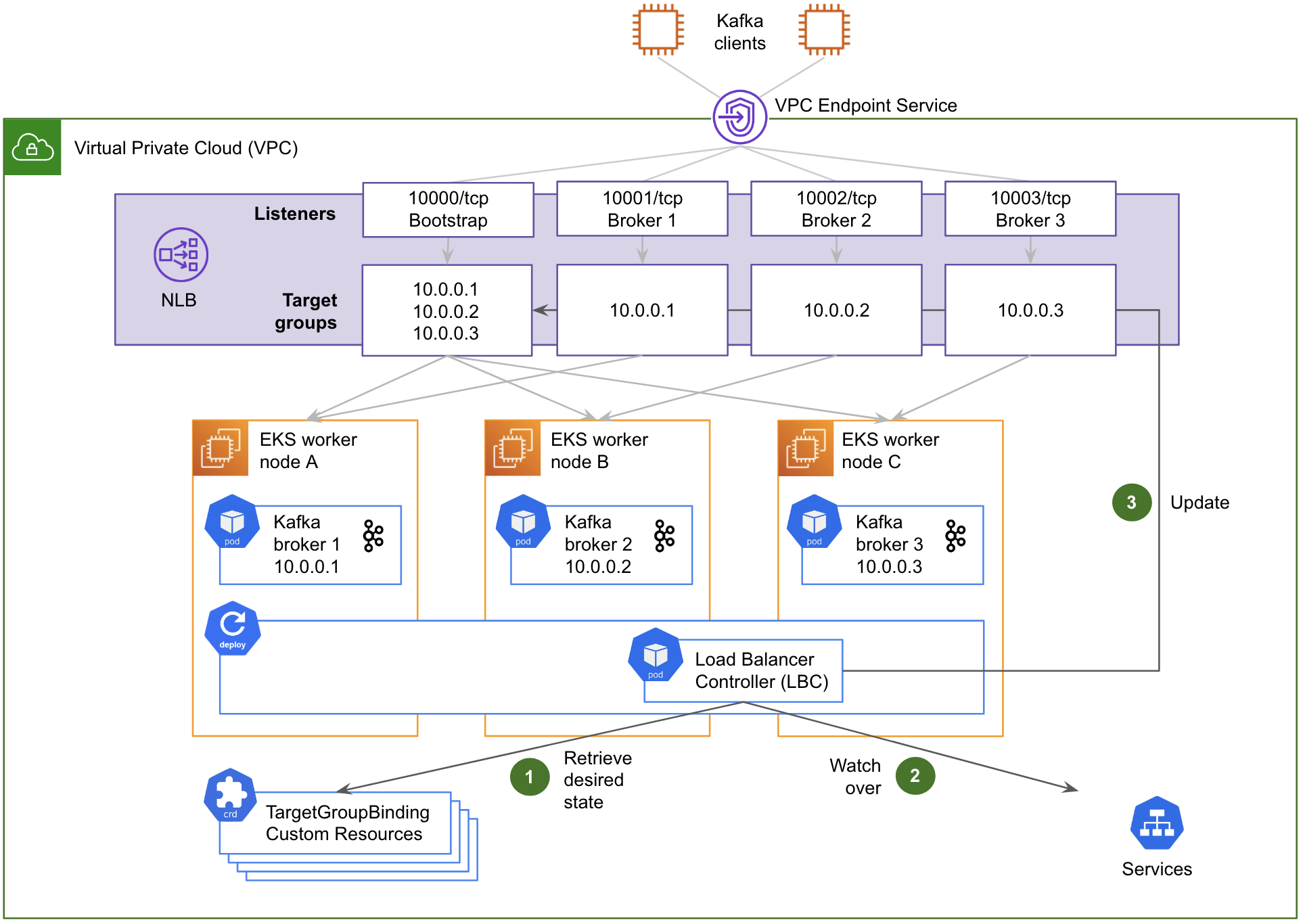
Dynamic NLB configuration
To automatically map the NLB’s target groups with a newly spun up EC2 instance, we leveraged the AWS Load Balancer Controller (LBC).
Let us see how it works.
Fig. 4 Architecture of the LBC managing the NLB’s target groups via TargetGroupBinding custom resources.
Fig. 4 shows how the LBC automates the reconfiguration of the NLB’s target groups:
It first retrieves the desired state described in Kubernetes custom resources (CR) of type TargetGroupBinding. There is one such resource per target group to maintain. Each TargetGroupBinding CR associates its respective target group with a Kubernetes service.
The LBC then watches over the changes of the Kubernetes services that are referenced in the TargetGroupBinding CRs’ definition, specifically the private IP addresses exposed by their respective Endpoints resources.
When a change is detected, it dynamically updates the corresponding NLB’s target groups with those IP addresses as well as the TCP port of the target containers (containerPort).
This automated design sets up the NLB’s target groups with IP addresses (targetType: ip) instead of EC2 instance IDs (targetType: instance). Although the LBC can handle both target types, the IP address approach is actually more straightforward in our case, since each pod has a routable private IP address in the AWS subnet, thanks to the AWS Container Networking Interface (CNI) plug-in.
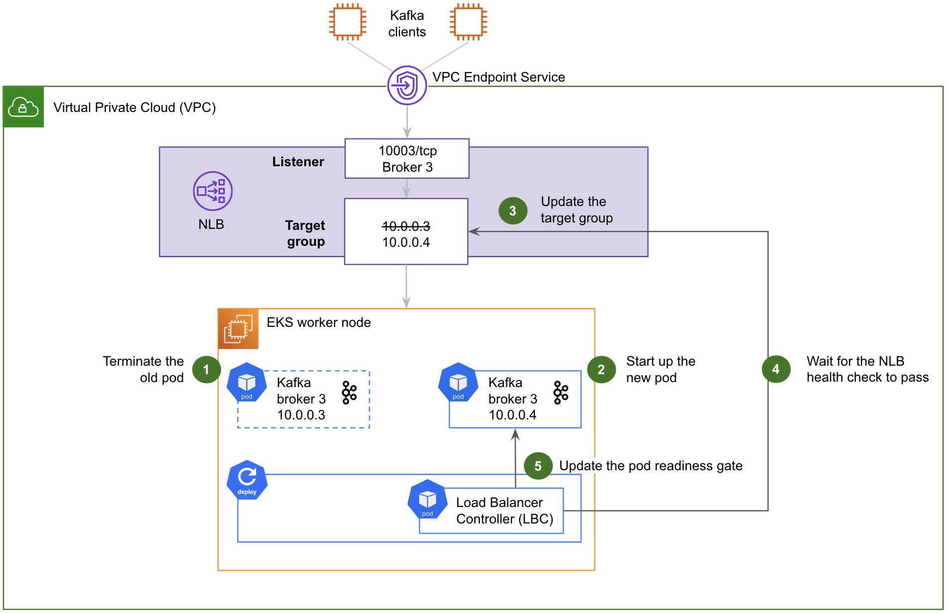
This dynamic NLB configuration design comes with a challenge. Whenever we need to update the Strimzi CR, the rollout of the change to each Kafka pod in a rolling update fashion is happening too fast for the NLB. This is because the NLB inherently takes some time to mark each target as healthy before enabling it. The Kafka brokers that have just been rolled out start advertising their broker-specific endpoints to the Kafka clients via the bootstrap service, but those
endpoints are actually not immediately available because the NLB is still checking their health. To mitigate this, we have reduced the HealthCheckIntervalSeconds and HealthyThresholdCount parameters of each target group to their minimum values of 5 and 2 respectively. This reduces the maximum delay for the NLB to detect that a target has become healthy to 10 seconds. In addition, we have configured the LBC with a Pod Readiness Gate. This feature makes the Strimzi rolling deployment wait for the health check of the NLB to pass, before marking the current pod as Ready and proceeding with the next pod.
Fig. 5 Steps for a Strimzi rolling deployment with a Pod Readiness Gate. Only one Kafka broker and one NLB listener and target group are shown for simplicity.
Fig. 5 shows how the Pod Readiness Gate works during a Strimzi rolling deployment:
The old Kafka pod is terminated.
The new Kafka pod starts up and joins the Kafka cluster. Its individual endpoint for direct access via the NLB is immediately advertised by the Kafka cluster. However, at this stage, it is not reachable, as the target group of the NLB still points to the IP address of the old Kafka pod.
The LBC updates the target group of the NLB with the IP address of the new Kafka pod, but the NLB health check has not yet passed, so the traffic is not forwarded to the new Kafka pod just yet.
The LBC then waits for the NLB health check to pass, which takes 10 seconds. Once the NLB health check has passed, the NLB resumes forwarding the traffic to the Kafka pod.
Finally, the LBC updates the pod readiness gate of the new Kafka pod. This informs Strimzi that it can proceed with the next pod of the rolling deployment.
Data persistence with EBS
To address the challenge of the residual PV and PVC of the old worker node preventing Kubernetes from mounting the local storage of the new worker node after a node rotation, we adopted Elastic Block Store (EBS) volumes instead of NVMe instance store volumes. Contrary to the latter, EBS volumes can conveniently be attached and detached. The trade-off is that their performance is significantly lower.
However, relying on EBS comes with additional benefits:
The cost per GB is lower, compared to NVMe instance store volumes.
Using EBS decouples the size of an instance in terms of CPU and memory from its storage capacity, leading to further cost savings by independently right-sizing the instance type and its storage. Such a separation of concerns also opens the door to new use cases requiring disproportionate amounts of storage.
After a worker node rotation, the time needed for the new node to get back in sync is faster, as it only needs to catch up the data that was produced during the downtime. This leads to shorter maintenance operations and higher iteration speed. Incidentally, the associated inter-AZ traffic cost is also lower, since there is less data to transfer among brokers during this time.
Increasing the storage capacity is an online operation.
Data backup is supported by taking snapshots of EBS volumes.
We have verified with our historical monitoring data that the performance of EBS General Purpose 3 (gp3) volumes is significantly above our maximum historical values for both throughput and I/O per second (IOPS), and we have successfully benchmarked a test EBS-based Kafka cluster. We have also set up new monitors to be alerted in case we need to
provision either additional throughput or IOPS, beyond the baseline of EBS gp3 volumes.
With that, we updated our instance types from storage optimised instances to either general purpose or memory optimised instances. We added the Amazon EBS Container Storage Interface (CSI) driver to the Kubernetes cluster and created a new Kubernetes storage class to let the cluster dynamically provision EBS gp3 volumes.
We configured Strimzi to use that storage class to create any new PVCs. This makes Strimzi able to automatically create the EBS volumes it needs, typically when the cluster is first set up, but also to attach/detach the volumes to/from the EC2 instances whenever a Kafka pod is relocated to a different worker node.
Note that the EBS volumes are not part of any ASG Launch Template, nor do they scale automatically with the ASGs.
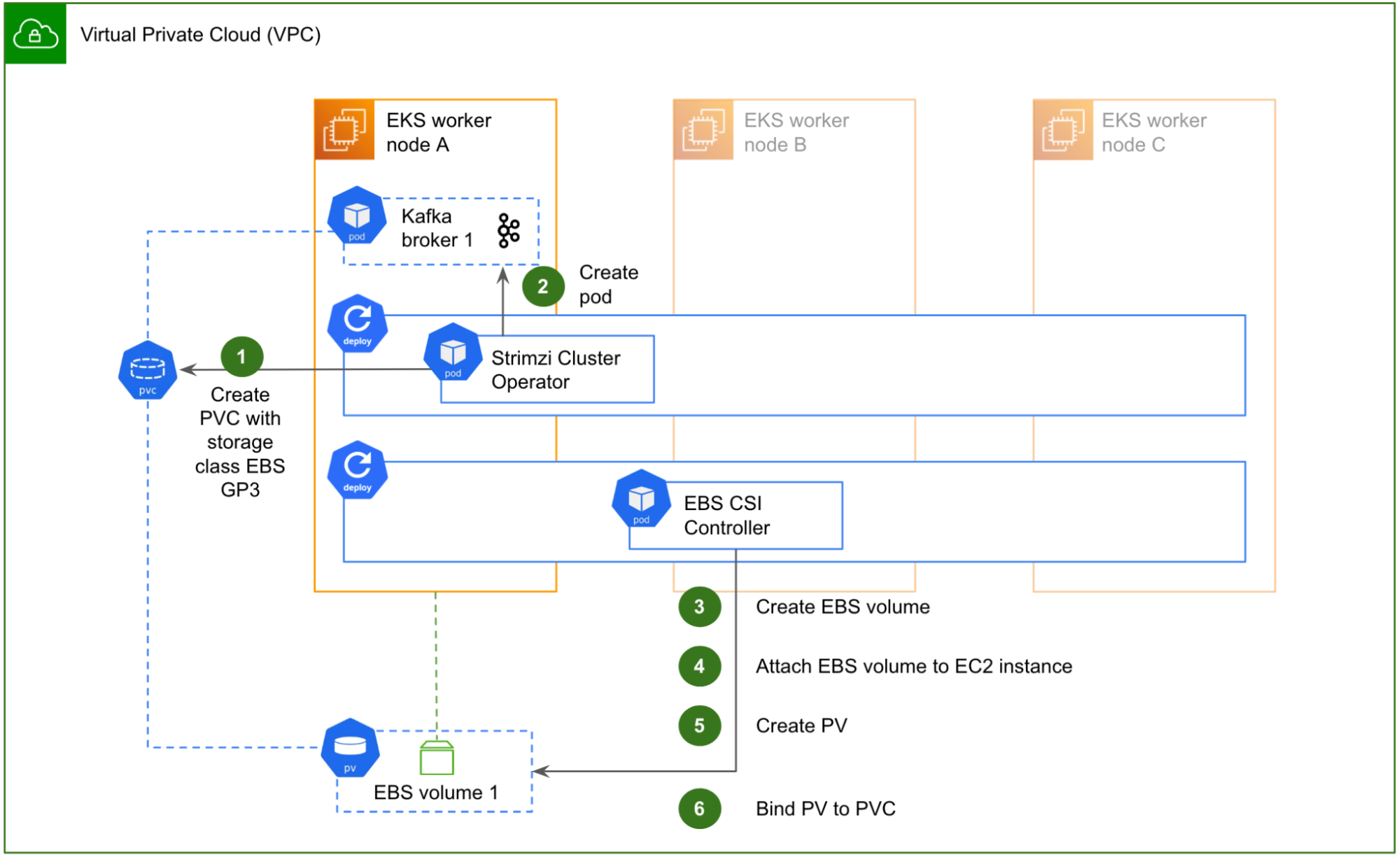
Fig. 6 Steps for the Strimzi Operator to create an EBS volume and attach it to a new Kafka pod.
Fig. 6 illustrates how this works when Strimzi sets up a new Kafka broker, for example the first broker of the cluster in the initial setup:
The Strimzi Cluster Operator first creates a new PVC, specifying a volume size and EBS gp3 as its storage class. The storage class is configured with the EBS CSI Driver as the volume provisioner, so that volumes are dynamically provisioned [1]. However, because it is also set up with volumeBindingMode: WaitForFirstConsumer, the volume is not yet provisioned until a pod actually claims the PVC.
The Strimzi Cluster Operator then creates the Kafka pod, with a reference to the newly created PVC. The pod is scheduled to start, which in turn claims the PVC.
This triggers the EBS CSI Controller. As the volume provisioner, it dynamically creates a new EBS volume in the AWS VPC, in the AZ of the worker node where the pod has been scheduled to start.
It then attaches the newly created EBS volume to the corresponding EC2 instance.
After that, it creates a Kubernetes PV with nodeAffinity and claimRef specifications, making sure that the PV is reserved for the Kafka broker 1 pod.
Lastly, it updates the PVC with the reference of the newly created PV. The PVC is now in Bound state and the Kafka pod can start.
One important point to take note of is that EBS volumes can only be attached to EC2 instances residing in their own AZ. Therefore, when rotating a worker node, the EBS volume can only be re-attached to the new instance if both old and new instances reside in the same AZ. A simple way to guarantee this is to set up one ASG per AZ, instead of a single ASG spanning across 3 AZs.
Also, when such a rotation occurs, the new broker only needs to synchronise the recent data produced during the brief downtime, which is typically an order of magnitude faster than replicating the entire volume (depending on the overall retention period of the hosted Kafka topics).
Table 1 Comparison of the resynchronization of the Kafka data after a broker rotation between the initial design and the new design with EBS volumes.
Initial design (NVMe instance store volumes)
New design (EBS volumes)
Data to synchronise
All of the data
Recent data produced during the brief downtime
Function of (primarily)
Retention period
Downtime
Typical duration
Hours
Minutes
Outcome
With all that, let us revisit the initial scenario, where a malfunctioning worker node is being replaced by a fresh new node.
Fig. 7 Representation of a worker node termination after implementing the solution. Node C is terminated and replaced by node D. This time, the Kafka broker 3 pod is able to start and serve traffic.
Fig. 7 shows the worker node C being terminated and replaced (by the ASG) by a new worker node D, similar to what we have described in the initial problem statement. The worker node D automatically joins the Kubernetes cluster on start-up.
However, this time, a seamless failover takes place:
The Kafka clients that were in the middle of producing or consuming to/from the partition leaders of Kafka broker 3 are gracefully redirected to Kafka brokers 1 and 2, where Kafka has migrated the leadership of its leader partitions.
The target groups of the NLB for both the bootstrap connection and Kafka broker 3 are automatically updated by the LBC. The connectivity between the NLB and Kafka broker 3 is immediately restored.
Triggered by the creation of the Kafka broker 3 pod, the Amazon EBS CSI driver running on the worker node D re-attaches the EBS volume 3 that was previously attached to the worker node C, to the worker node D instead. This enables Kubernetes to automatically re-bind the corresponding PV and PVC to Kafka broker 3 pod. With its storage dependency resolved, Kafka broker 3 is able to start successfully and re-join the Kafka cluster. From there, it only needs to catch up with the new data that was produced
during its short downtime, by replicating it from Kafka brokers 1 and 2.
With this fault-tolerant design, when an EC2 instance is being retired by AWS, no particular action is required from our end.
Similarly, our EKS version upgrades, as well as any operations that require rotating all worker nodes of the cluster in general, are:
Simpler and less error-prone: We only need to rotate each instance in sequence, with no need for manually reconfiguring the target groups of the NLB and deleting the zombie PVCs anymore.
Faster: The time between each instance rotation is limited to the short amount of time it takes for the restarted Kafka broker to catch up with the new data.
More cost-efficient: There is less data to transfer across AZs (which is charged by AWS).
It is worth noting that we have chosen to omit Zookeeper and Cruise Control in this article, for the sake of clarity and simplicity. In reality, all pods in the Kubernetes cluster – including Zookeeper and Cruise Control – now benefit from the same graceful stop, triggered by the AWS termination events and the NTH. Similarly, the EBS CSI driver improves the fault tolerance of any pods that use EBS volumes for persistent storage, which includes the Zookeeper pods.
Challenges faced
One challenge that we are facing with this design lies in the EBS volumes’ management.
On the one hand, the size of EBS volumes cannot be increased consecutively before the end of a cooldown period (minimum of 6 hours and can exceed 24 hours in some cases [2]). Therefore, when we need to urgently extend some EBS volumes because the size of a Kafka topic is suddenly growing, we need to be relatively generous when sizing the new required capacity and add a comfortable security margin, to make sure that we are not running out of storage in the short run.
On the other hand, shrinking a Kubernetes PV is not a supported operation. This can affect the cost efficiency of our design if we overprovision the storage capacity by too much, or in case the workload of a particular cluster organically diminishes.
One way to mitigate this challenge is to tactically scale the cluster horizontally (ie. adding new brokers) when there is a need for more storage and the existing EBS volumes are stuck in a cooldown period, or when the new storage need is only temporary.
What’s next?
In the future, we can improve the NTH’s capability by utilising webhooks. Upon receiving events from SQS, the NTH can also forward the events to the specified webhook URLs.
This can potentially benefit us in a few ways, e.g.:
Proactively spinning up a new instance without waiting for the old one to be terminated, whenever a termination event is received. This would shorten the rotation time even further.
Sending Slack notifications to Coban engineers to keep them informed of any actions taken by the NTH.
We would need to develop and maintain an application that receives webhook events from the NTH and performs the necessary actions.
In addition, we are also rolling out Karpenter to replace the Kubernetes Cluster Autoscaler, as it is able to spin up new instances slightly faster, helping reduce the four minutes delay a Kafka pod remains in Pending state during a node rotation. Incidentally, Karpenter also removes the need for setting up one ASG by AZ, as it is able to deterministically provision instances in a specific AZ, for example where a particular EBS volume resides.
Lastly, to ensure that the performance of our EBS gp3 volumes is both sufficient and cost-efficient, we want to explore autoscaling their throughput and IOPS beyond the baseline, based on the usage metrics collected by our monitoring stack.
We would like to thank our team members and Grab Kubernetes gurus that helped review and improve this blog before publication: Will Ho, Gable Heng, Dewin Goh, Vinnson Lee, Siddharth Pandey, Shi Kai Ng, Quang Minh Tran, Yong Liang Oh, Leon Tay, Tuan Anh Vu.
Join us
Grab is the leading superapp platform in Southeast Asia, providing everyday services that matter to consumers. More than just a ride-hailing and food delivery app, Grab offers a wide range of on-demand services in the region, including mobility, food, package and grocery delivery services, mobile payments, and financial services across 428 cities in eight countries.
Powered by technology and driven by heart, our mission is to drive Southeast Asia forward by creating economic empowerment for everyone. If this mission speaks to you, join our team today!
Coban is Grab’s real-time data streaming platform team. As a platform team, we thrive on providing our internal users from all verticals with self-served data-streaming resources, such as Kafka topics, Flink and Change Data Capture (CDC) pipelines, various kinds of Kafka-Connect connectors, as well as Apache Zeppelin notebooks, so that they can effortlessly leverage real-time data to build intelligent applications and services.
In this article, we present our journey from pure Infrastructure-as-Code (IaC) towards a more sophisticated control plane that has revolutionised the way data streaming resources are self-served at Grab. This change also leads to improved scalability, stability, security, and user adoption of our data streaming platform.
Problem statement
In the early ages of public cloud, it was a common practice to create virtual resources by clicking through the web console of a cloud provider, which is sometimes referred to as ClickOps.
ClickOps has many downsides, such as:
Inability to review, track, and audit changes to the infrastructure.
Inability to massively scale the infrastructure operations.
Inconsistencies between environments, e.g. staging and production.
Inability to quickly recover from a disaster by re-creating the infrastructure at a different location.
That said, ClickOps has one tremendous advantage; it makes creating resources using a graphical User Interface (UI) fairly easy for anyone like Infrastructure Engineers, Software Engineers, Data Engineers etc. This also leads to a high iteration speed towards innovation in general.
IaC resolved many of the limitations of ClickOps, such as:
Changes are committed to a Version Control System (VCS) like Git: They can be reviewed by peers before being merged. The full history of all changes is available for investigating issues and for audit.
The infrastructure operations scale better: Code for similar pieces of infrastructure can be modularised. Changes can be rolled out automatically by Continuous Integration (CI) pipelines in the VCS system, when a change is merged to the main branch.
The same code can be used to deploy the staging and production environments consistently.
The infrastructure can be re-created anytime from its source code, in case of a disaster.
However, IaC unwittingly posed a new entry barrier too, requiring the learning of new tools like Ansible, Puppet, Chef, Terraform, etc.
Some organisations set up dedicated Site Reliability Engineer (SRE) teams to centrally manage, operate, and support those tools and the infrastructure as a whole, but that soon created the potential of new bottlenecks in the path to innovation.
On the other hand, others let engineering teams manage their own infrastructure, and Grab adopted that same approach. We use Terraform to manage infrastructure, and all teams are expected to have select engineers who have received Terraform training and have a clear understanding of it.
In this context, Coban’s platform initially started as a handful of Git repositories where users had to submit their Merge Requests (MR) of Terraform code to create their data streaming resources. Once reviewed by a Coban engineer, those Terraform changes would be applied by a CI pipeline running Atlantis.
While this was a meaningful first step towards self-service and platformisation of Coban’s offering within Grab, it had several significant downsides:
Stability: Due to the lack of control on the Terraform changes, the CI pipeline was prone to human errors and frequent failures. For example, users would initiate a new Terraform project by duplicating an existing one, but then would forget to change the location of the remote Terraform state, leading to the in-place replacement of an existing resource.
Scalability: The Coban team needed to review all MRs and provide ad hoc support whenever the pipeline failed.
Security: In the absence of Identity and Access Management (IAM), MRs could potentially contain changes pertaining to other teams’ resources, or even changes to Coban’s core infrastructure, with code review as the only guardrail.
Limited user growth: We could only acquire users who were well-versed in Terraform.
It soon became clear that we needed to build a layer of abstraction between our users and the Terraform code, to increase the level of control and lower the entry barrier to our platform, while still retaining all of the benefits of IaC under the hood.
Solution
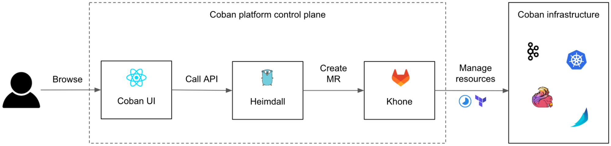
We designed and built an in-house three-tier control plane made of:
Coban UI, a front-end web interface, providing our users with a seamless ClickOps experience.
Heimdall, the Go back-end of the web interface, transforming ClickOps into IaC.
Khone, the storage and provisioner layer, a Git repository storing Terraform code and metadata of all resources as well as the CI pipelines to plan and apply the changes.
In the next sections, we will deep dive in those three components.
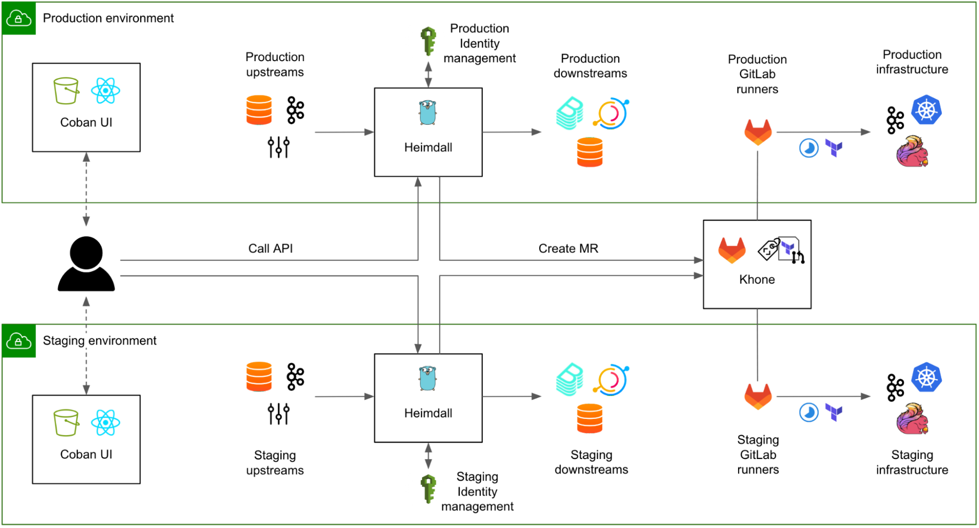
Fig. 1 Simplified architecture of a request flowing from the user to the Coban infrastructure, via the three components of the control plane: the Coban UI, Heimdall, and Khone.
Although we designed the user journey to start from the Coban UI, our users can still opt to communicate with Heimdall and with Khone directly, e.g. for batch changes, or just because many engineers love Git and we want to encourage broad adoption. To make sure that data is eventually consistent across the three systems, we made Khone the only persistent storage layer. Heimdall regularly fetches data from Khone, caches it, and presents it to the Coban UI upon each query.
We also continued using Terraform for all resources, instead of mixing various declarative infrastructure approaches (e.g. Kubernetes Custom Resource Definition, Helm charts), for the sake of consistency of the logic in Khone’s CI pipelines.
Coban UI
The Coban UI is a ReactSingle Page Application (React SPA) designed by our partner team Chroma, a dedicated team of front-end engineers who thrive on building legendary UIs and reusable components for platform teams at Grab.
It serves as a comprehensive self-service portal, enabling users to effortlessly create data streaming resources by filling out web forms with just a few clicks.
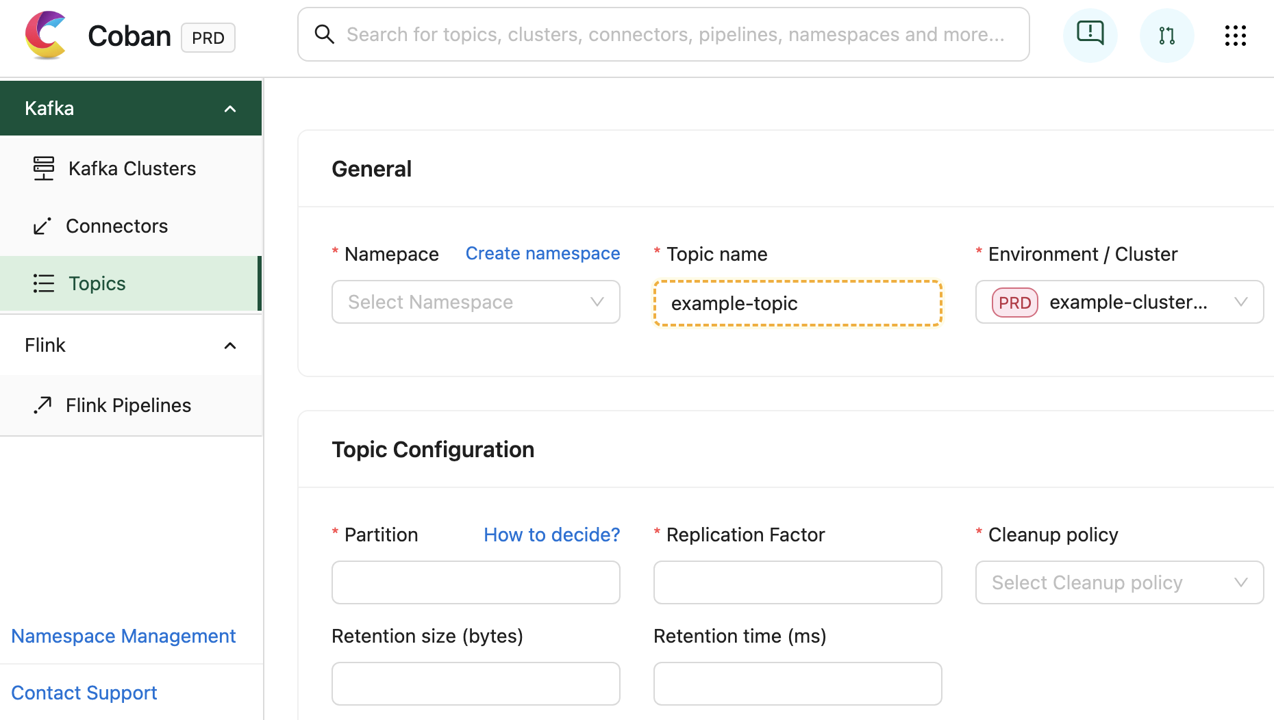
Fig. 2 Screen capture of a new Kafka topic creation in the Coban UI.
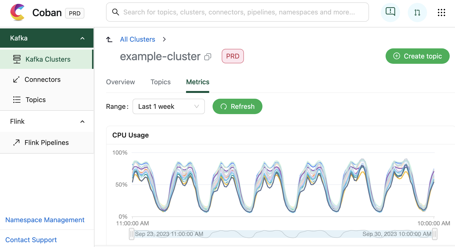
In addition to facilitating resource creation and configuration, the Coban UI is seamlessly integrated with multiple monitoring systems. This integration allows for real-time monitoring of critical metrics and health status for Coban infrastructure components, including Kafka clusters, Kafka topic bytes in/out rates, and more. Under the hood, all this information is exposed by Heimdall APIs.
Fig. 3 Screen capture of the metrics of a Kafka cluster in the Coban UI.
In terms of infrastructure, the Coban UI is hosted in AWS S3 website hosting. All dynamic content is generated by querying the APIs of the back-end: Heimdall.
Heimdall
Heimdall is the Go back-end of the Coban UI. It serves a collection of APIs for:
Managing the data streaming resources of the Coban platform with Create, Read, Update and Delete (CRUD) operations, treating the Coban UI as a first-class citizen.
Exposing the metadata of all Coban resources, so that they can be used by other platforms or searched in the Coban UI.
In the next sections, we are going to dive deeper into these two features.
Managing the data streaming resources
First and foremost, Heimdall enables our users to self-manage their data streaming resources. It primarily relies on Khone as its storage and provisioner layer for actual resource management via Git CI pipelines. Therefore, we designed Heimdall’s resource management workflow to leverage the underlying Git flow.
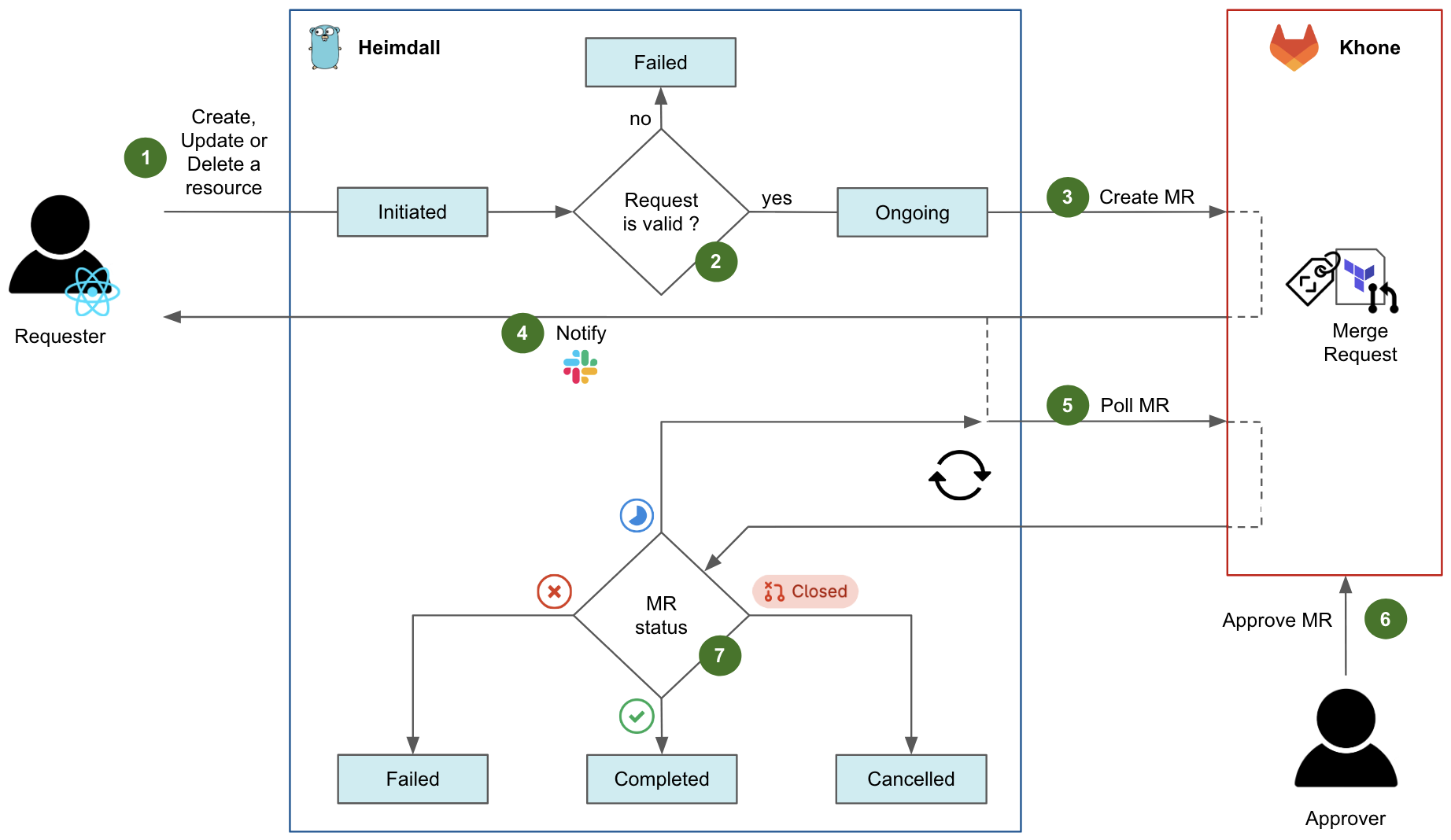
Fig. 4 Diagram flow of a request in Heimdall.
Fig. 4 shows the diagram flow of a typical request in Heimdall to create, update, or delete a resource.
An authenticated user initiates a request, either by navigating in the Coban UI or by calling the Heimdall API directly. At this stage, the request state is Initiated on Heimdall.
Heimdall validates the request against multiple validation rules. For example, if an ongoing change request exists for the same resource, the request fails. If all tests succeed, the request state moves to Ongoing.
Heimdall then creates an MR in Khone, which contains the Terraform files describing the desired state of the resource, as well as an in-house metadata file describing the key attributes of both resource and requester.
After the MR has been created successfully, Heimdall notifies the requester via Slack and shares the MR URL.
After that, Heimdall starts polling the status of the MR in a loop.
For changes pertaining to production resources, an approver who is code owner in the repository of the resource has to approve the MR. Typically, the approver is an immediate teammate of the requester. Indeed, as a platform team, we empower our users to manage their own resources in a self-service fashion. Ultimately, the requester would merge the MR to trigger the CI pipeline applying the actual Terraform changes. Note that for staging resources, this entire step 6 is automatically performed by Heimdall.
Depending on the MR status and the status of its CI pipeline in Khone, the final state of the request can be:
Failed if the CI pipeline has failed in Khone.
Completed if the CI pipeline has succeeded in Khone.
Cancelled if the MR was closed in Khone.
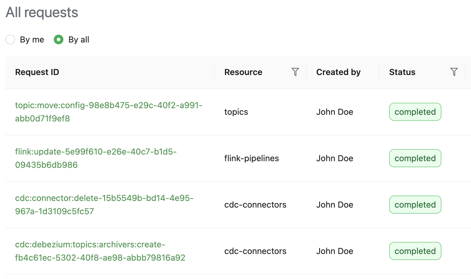
Heimdall exposes APIs to let users track the status of their requests. In the Coban UI, a page queries those APIs to elegantly display the requests.
Fig. 5 Screen capture of the Coban UI showing all requests.
Exposing the metadata
Apart from managing the data streaming resources, Heimdall also centralises and exposes the metadata pertaining to those resources so other Grab systems can fetch and use it. They can make various queries, for example, listing the producers and consumers of a given Kafka topic, or determining if a database (DB) is the data source for any CDC pipeline.
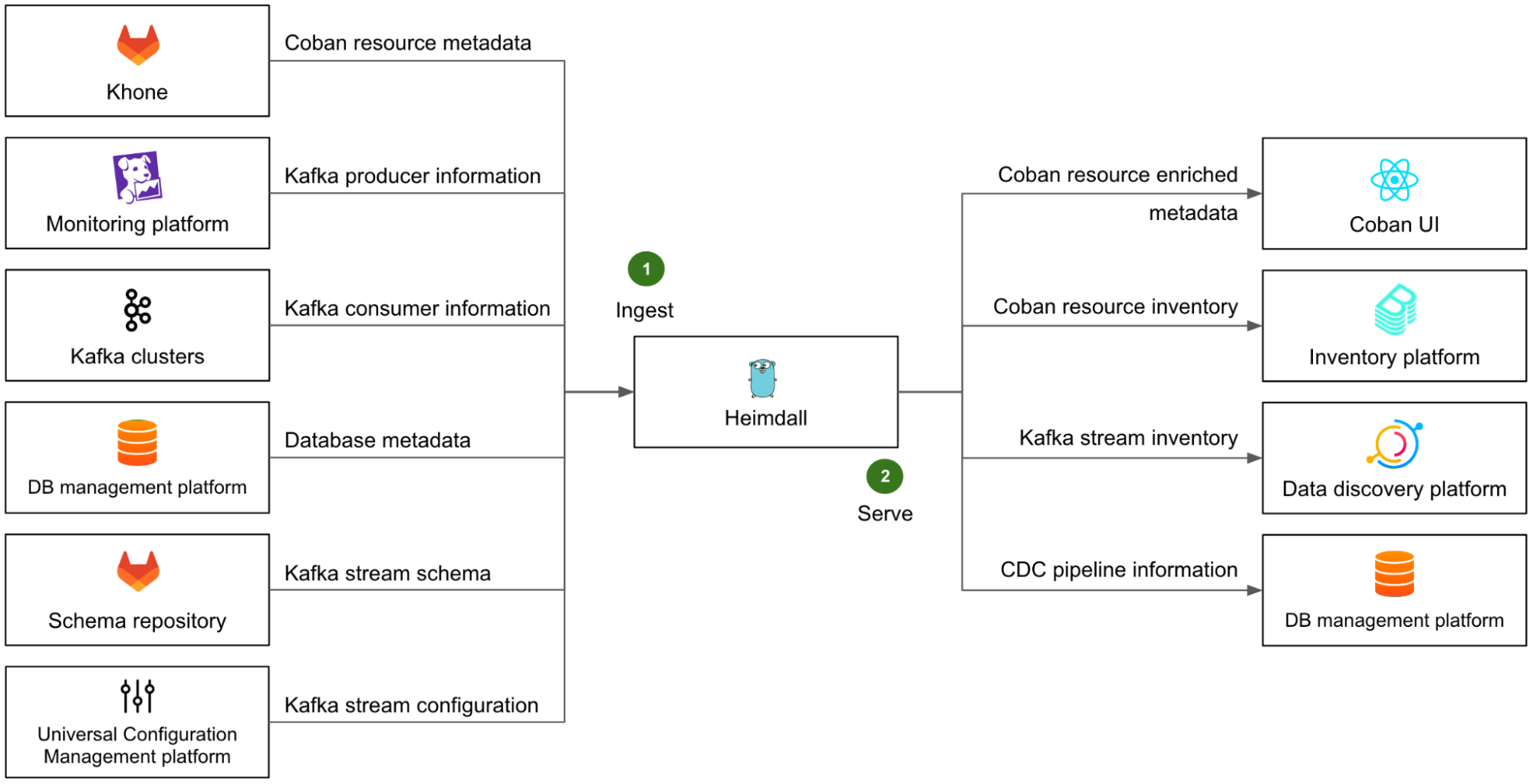
To make this happen, Heimdall not only retains the metadata of all of the resources that it creates, but also regularly ingests additional information from a variety of upstream systems and platforms, to enrich and make this metadata comprehensive.
Fig. 6 Diagram showing some of Heimdall’s upstreams (on the left) and downstreams (on the right) for metadata collection, enrichment, and serving. The arrows show the data flow. The network connection (client -> server) is actually the other way around.
On the left side of Fig. 6, we illustrate Heimdall’s ingestion mechanism with several examples (step 1):
The metadata of all Coban resources is ingested from Khone. This means the metadata of the resources that were created directly in Khone is also available in Heimdall.
The list of Kafka producers is retrieved from our monitoring platform, where most of them emit metrics.
The list of Kafka consumers is retrieved directly from the respective Kafka clusters, by listing the consumer groups and respective Client IDs of each partition.
The metadata of all DBs, that are used as a data source for CDC pipelines, is fetched from Grab’s internal DB management platform.
The Kafka stream schemas are retrieved from the Coban schema repository.
The Kafka stream configuration of each stream is retrieved from Grab Universal Configuration Management platform.
With all of this ingested data, Heimdall can provide comprehensive and accurate information about all data streaming resources to any other Grab platforms via a set of dedicated APIs.
The right side of Fig. 6 shows some examples (step 2) of Heimdall’s serving mechanism:
As a downstream of Heimdall, the Coban UI enables our direct users to conveniently browse their data streaming resources and access their attributes.
The entire resource inventory is ingested into the broader Grab inventory platform, based on backstage.io.
The Kafka streams are ingested into Grab’s internal data discovery platform, based on DataHub, where users can discover and trace the lineage of any piece of data.
The CDC connectors pertaining to DBs are ingested by Grab internal DB management platform, so that they are made visible in that platform when users are browsing their DBs.
Note that the downstream platforms that ingest data from Heimdall each expose a particular view of the Coban inventory that serves their purpose, but the Coban platform remains the only source of truth for any data streaming resource at Grab.
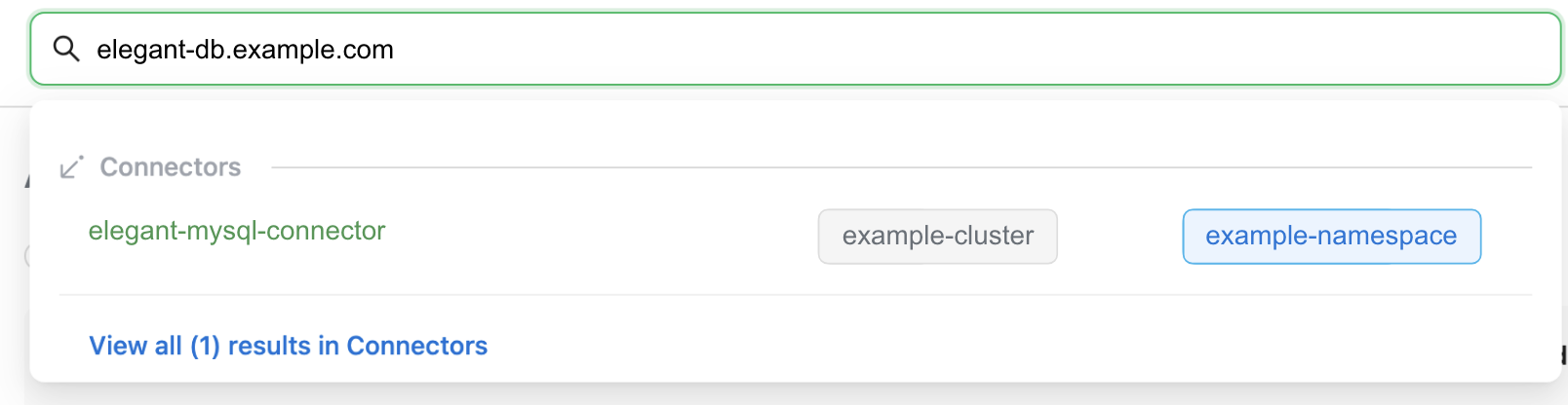
Lastly, Heimdall leverages an internal MySQL DB to support quick data query and exploration. The corresponding API is called by the Coban UI to let our users conveniently search globally among all resources’ attributes.
Fig. 7 Screen capture of the global search feature in the Coban UI.
Khone
Khone is the persistent storage layer of our platform, as well as the executor for actual resource creation, changes, and deletion. Under the hood, it is actually a GitLab repository of Terraform code in typical GitOps fashion, with CI pipelines to plan and apply the Terraform changes automatically. In addition, it also stores a metadata file for each resource.
Compared to letting the platform create the infrastructure directly and keep track of the desired state in its own way, relying on a standard IaC tool like Terraform for the actual changes to the infrastructure presents two major advantages:
The Terraform code can directly be used for disaster recovery. In case of a disaster, any entitled Cobaner with a local copy of the main branch of the Khone repository is able to recreate all our platform resources directly from their machine. There is no need to rebuild the entire platform’s control plane, thus reducing our Recovery Time Objective (RTO).
Minimal effort required to follow the API changes of our infrastructure ecosystem (AWS, Kubernetes, Kafka, etc.). When such a change happens, all we need to do is to update the corresponding Terraform provider.
If you’d like to read more about Khone, check out Securing GitOps pipelines. In this section, we will only focus on Khone’s features that are relevant from the platform perspective.
Lightweight Terraform
In Khone, each resource is stored as a Terraform definition. There are two major differences from a normal Terraform project:
No Terraform environment, such as the required Terraform providers and the location of the remote Terraform state file. They are automatically generated by the CI pipeline via a simple wrapper.
Only vetted Khone Terraform modules can be used. This is controlled and enforced by the CI pipeline via code inspection. There is one such Terraform module for each kind of supported resource of our platform (e.g. Kafka topic, Flink pipeline, Kafka Connect mirror source connector etc.). Furthermore, those in-house Terraform modules are designed to automatically derive their key variables (e.g. resource name, cluster name, environment) from the relative path of the parent Terraform project in the Khone repository.
Those characteristics are designed to limit the risk and blast radius of human errors. They also make sure that all resources created in Khone are supported by our platform, so that they can also be discovered and managed in Heimdall and the Coban UI. Lastly, by generating the Terraform environment on the fly, we can destroy resources simply by deleting the directory of the project in the code base – this would not be possible otherwise.
Resource metadata
All resource metadata is stored in a YAML file that is present in the Terraform directory of each resource in the Khone repository. This is mainly used for ownership and cost attribution.
With this metadata, we can:
Better communicate with our users whenever their resources are impacted by an incident or an upcoming maintenance operation.
Help teams understand the costs of their usage of our platform, a significant step towards cost efficiency.
There are two different ways resource metadata can be created:
Automatically through Heimdall: The YAML metadata file is automatically generated by Heimdall.
Through Khone by a human user: The user needs to prepare the YAML metadata file and include it in the MR. This file is then verified by the CI pipeline.
Outcome
The initial version of the three-tier Coban platform, as described in this article, was internally released in March 2022, supporting only Kafka topic management at the time. Since then, we have added support for Flink pipelines, four kinds of Kafka Connect connectors, CDC pipelines, and more recently, Apache Zeppelin notebooks. At the time of writing, the Coban platform manages about 5000 data streaming resources, all described as IaC under the hood.
Our platform also exposes enriched metadata that includes the full data lineage from Kafka producers to Kafka consumers, as well as ownership information, and cost attribution.
With that, our monthly active users have almost quadrupled, truly moving the needle towards democratising the usage of real-time data within all Grab verticals.
In spite of that user growth, the end-to-end workflow success rate for self-served resource creation, change or deletion, remained well above 90% in the first half of 2023, while the Heimdall API uptime was above 99.95%.
Challenges faced
A common challenge for platform teams resides in the misalignment between the Service Level Objective (SLO) of the platform, and the various environments (e.g. staging, production) of the managed resources and upstream/downstream systems and platforms.
Indeed, the platform aims to guarantee the same level of service, regardless of whether it is used to create resources in the staging or the production environment. From the platform team’s perspective, the platform as a whole is considered production-grade, as soon as it serves actual users.
A naive approach to address this challenge is to let the production version of the platform manage all resources regardless of their respective environments. However, doing so does not permit a hermetic segregation of the staging and production environments across the organisation, which is a good security practice, and often a requirement for compliance. For example, the production version of the platform would have to connect to upstream systems in the staging environment, e.g. staging Kafka clusters to collect their consumer groups, in the case of Heimdall. Conversely, the staging version of certain downstreams would have to connect to the production version of Heimdall, to fetch the metadata of relevant staging resources.
The alternative approach, generally adopted across Grab, is to instantiate all platforms in each environment (staging and production), while still considering both instances as production-grade and guaranteeing tight SLOs in both environments.
Fig. 8 Architecture of the Coban platform, broken down by environment.
In Fig. 8, both instances of Heimdall have equivalent SLOs. The caveat is that all upstream systems and platforms must also guarantee a strict SLO in both environments. This obviously comes with a cost, for example, tighter maintenance windows for the operations pertaining to the Kafka clusters in the staging environment.
A strong “platform” culture is required for platform teams to fully understand that their instance residing in the staging environment is not their own staging environment and should not be used for testing new features.
What’s next?
Currently, users creating, updating, or deleting production resources in the Coban UI (or directly by calling Heimdall API) receive the URL of the generated GitLab MR in a Slack message. From there, they must get the MR approved by a code owner, typically another team member, and finally merge the MR, for the requested change to be actually implemented by the CI pipeline.
Although this was a fairly easy way to implement a maker/checker process that was immediately compliant with our regulatory requirements for any changes in production, the user experience is not optimal. In the near future, we plan to bring the approval mechanism into Heimdall and the Coban UI, while still providing our more advanced users with the option to directly create, approve, and merge MRs in GitLab. In the longer run, we would also like to enhance the Coban UI with the output of the Khone CI jobs that include the Terraform plan and apply results.
There is another aspect of the platform that we want to improve. As Heimdall regularly polls the upstream platforms to collect their metadata, this introduces a latency between a change in one of those platforms and its reflection in the Coban platform, which can hinder the user experience. To refresh resource metadata in Heimdall in near real time, we plan to leverage an existing Grab-wide event stream, where most of the configuration and code changes at Grab are produced as events. Heimdall will soon be able to consume those events and update the metadata of the affected resources immediately, without waiting for the next periodic refresh.
Join us
Grab is the leading superapp platform in Southeast Asia, providing everyday services that matter to consumers. More than just a ride-hailing and food delivery app, Grab offers a wide range of on-demand services in the region, including mobility, food, package and grocery delivery services, mobile payments, and financial services across 428 cities in eight countries.
Powered by technology and driven by heart, our mission is to drive Southeast Asia forward by creating economic empowerment for everyone. If this mission speaks to you, join our team today!
Over the next few years, most content on Netflix will come from Netflix’s own Studio. From the moment a Netflix film or series is pitched and long before it becomes available on Netflix, it goes through many phases. This happens at an unprecedented scale and introduces many interesting challenges; one of the challenges is how to provide visibility of Studio data across multiple phases and systems to facilitate operational excellence and empower decision making. Netflix is known for its loosely coupled microservice architecture and with a global studio footprint, surfacing and connecting the data from microservices into a studio data catalog in real time has become more important than ever.
Operational Reporting is a reporting paradigm specialized in covering high-resolution, low-latency data sets, serving detailed day-to-day activities¹ and processes of a business domain. Such a paradigm aspires to assist front-line operations personnel and stakeholders in “running the business”²; performing their tasks through means such as ad hoc analysis, decision-support, and tracking (of tasks, assets, schedules, etc). The paradigm spans across methods, tools, and technologies and is usually defined in contrast to analytical reporting and predictive modeling which are more strategic (vs. tactical) in nature.
At Netflix Studio, teams build various views of business data to provide visibility for day-to-day decision making. With dependable near real-time data, Studio teams are able to track and react better to the ever-changing pace of productions and improve efficiency of global business operations using the most up-to-date information. Data connectivity across Netflix Studio and availability of Operational Reporting tools also incentivizes studio users to avoid forming data silos.
The Journey
In the past few years, Netflix Studio has gone through few iterations of data movement approaches. In the initial stage, data consumers set up ETL pipelines directly pulling data from databases. With this batch style approach, several issues have surfaced like data movement is tightly coupled with database tables, database schema is not an exact mapping of business data model, and data being stale given it is not real time etc. Later on, we moved to event driven streaming data pipelines (powered by Delta), which solved some problems compared to the batch style, but had its own pain points, such as a high learning curve of stream processing technologies, manual pipeline setup, a lack of schema evolution support, inefficiency of onboarding new entities, inconsistent security access models, etc.
With the latest Data Mesh Platform, data movement in Netflix Studio reaches a new stage. This configuration driven platform decreases the significant lead time when creating a new pipeline, while offering new support features like end-to-end schema evolution, self-serve UI and secure data access. The high level diagram below indicates the latest version of data movement for Operational Reporting.
Operational Reporting Architecture Overview
For data delivery, we leverage the Data Mesh platform to power the data movement. Netflix Studio applications expose GraphQL queries via Studio Edge, which is a unified graph that connects all data in Netflix Studio and provides consistent data retrieval. Change Data Capture(CDC) source connector reads from studio applications’ database transaction logs and emits the change events. The CDC events are passed on to the Data Mesh enrichment processor, which issues GraphQL queries to Studio Edge to enrich the data. Once the data has landed in the Iceberg tables in Netflix Data Warehouse, they could be used for ad-hoc or scheduled querying and reporting. Centralized data will be moved to third party services such as Google Sheets and Airtable for the stakeholders. We will deep dive into Data Delivery and Data Consumption in the following sections.
Data Delivery via Data Mesh
What is Data Mesh?
Data Mesh is a fully managed, streaming data pipeline product used for enabling Change Data Capture (CDC) use cases. In Data Mesh, users create sources and construct pipelines. Sources mimic the state of an externally managed source — as changes occur in the external source, corresponding CDC messages are produced to the Data Mesh source. Pipelines can be configured to transform and store data to externally managed sinks.
Data Mesh provides a drag-and-drop, self-service user interface for exploring sources and creating pipelines so that users can focus on delivering business value without having to worry about managing and scaling complex data streaming infrastructure.
CDC and data source
Change data capture or CDC, is a semantic for processing changes in a source for the purpose of replicating those changes to a sink. The table changes could be row changes (insert row, update row, delete row) or schema changes (add column, alter column, drop column). As of now, CDC sources have been implemented for data stores at Netflix (MySQL, Postgres). CDC events can also be sent to Data Mesh via a Java Client Producer Library.
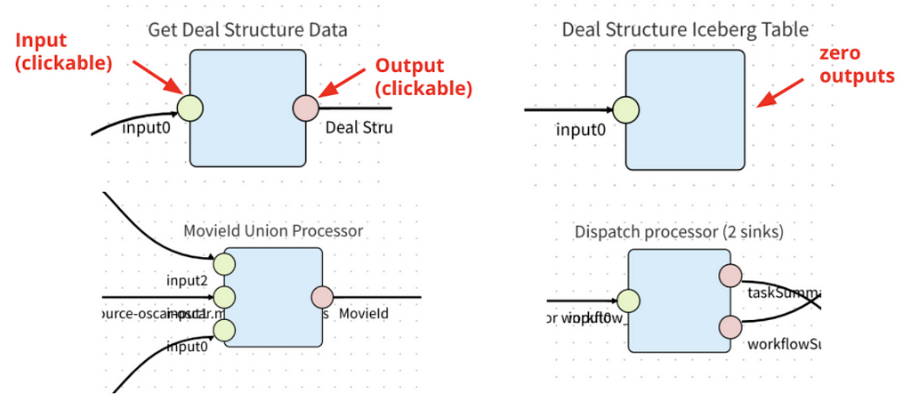
Reusable Processors and Configuration Driven
In Data Mesh, a processor is a configurable data processing application that consumes, transforms, and produces CDC events. A processor has 1 or more inputs and 0 or more outputs. Processors with 0 outputs are sink connectors; which write events to externally managed sinks (e.g. Iceberg, ElasticSearch, etc).
Processors with Different Inputs/Outputs
Data Mesh allows developers to contribute processors to the platform. Processors are not necessarily centrally developed and managed. However, the Data Mesh platform team strives to provide and manage the most highly leveraged processors (e.g. source connectors and sink connectors)
Processors are reusable. The same processor image package is used multiple times for all instances of the processor. Each instance is configured to fit each use case. For example, a GraphQL enrichment processor can be provisioned to query GraphQL Services to enrich data in different pipelines; an Iceberg sink processor can be initialized multiple times to write data to different databases/tables with different schema.
End-to-End Schema Evolution
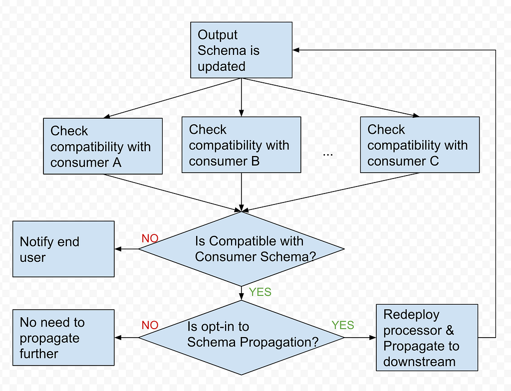
Schema is a key component of Data Mesh. When an upstream schema evolves (e.g. schema change in the MySQL table), Data Mesh detects the change, checks the compatibility and applies the change to the downstream. With schema evolution, Data Mesh ensures the Operational Reporting pipelines always produce data with the latest schema.
We will cover a few core concepts in the Data Mesh Schema domain.
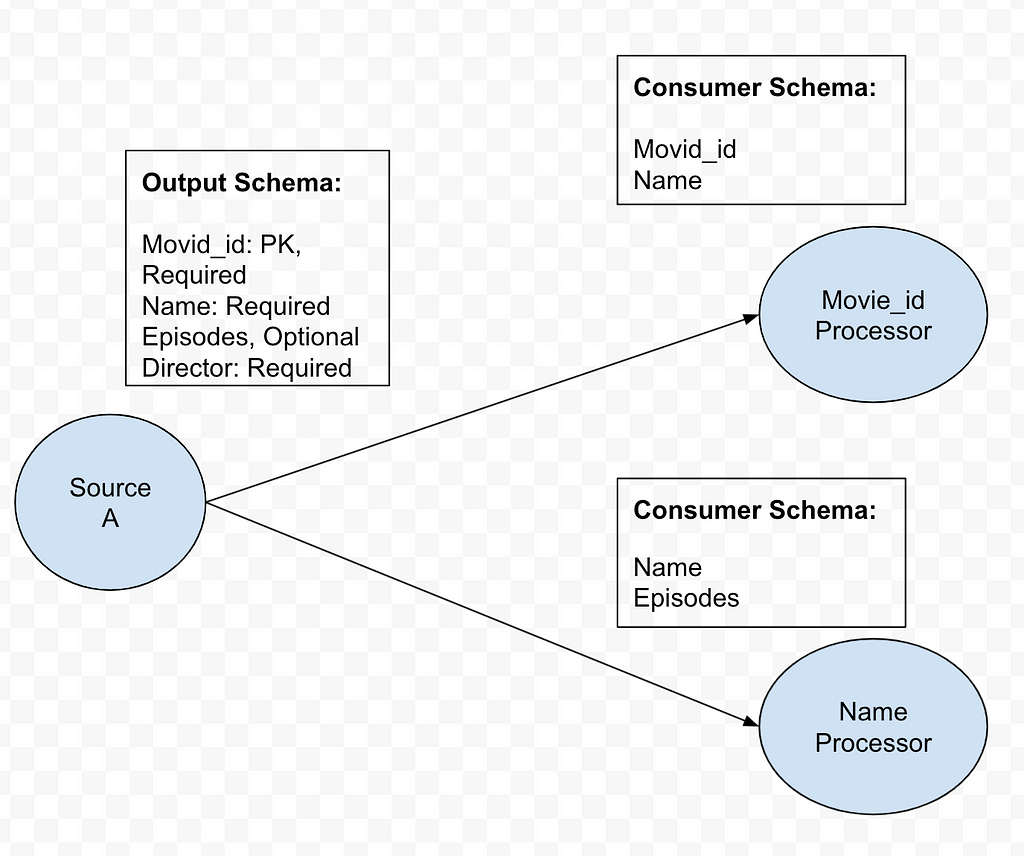
Consumer schema Consumer schema defines how data is consumed by the downstream processors. See example below.
Consumer Schema Example
Schema Compatibility Data Mesh uses Consumer Schema compatibility to achieve flexible yet safe schema evolution. If a field consumed by an Operational Reporting pipeline is removed from CDC source, Data Mesh categorizes this change as incompatible, pauses the pipeline processing and notifies the pipeline owner. On the other hand, if a required field is not consumed by any consumer, dropping such fields would be compatible.
Two Types of Processors 1. Pass through all fields from upstream to downstream.
Example: Filter Processor, Sink Processors
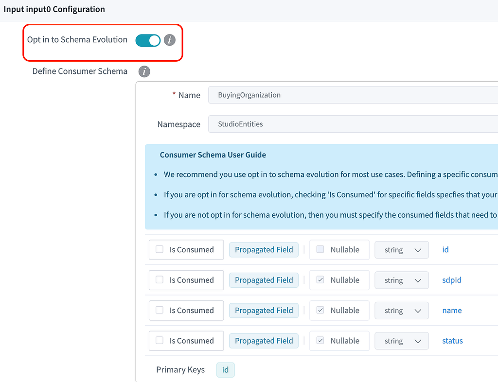
Opt in to schema Evolution example
2. Only uses a subset of fields from upstream.
Example: Project Processor, Enrichment Processor
Opt out to schema Evolution example
In Data Mesh, we introduce theOpt-in to Schema Evolution boolean flag to differentiate those two types of use cases.
Opt in: All the upstream fields will be propagated to the processor. For example, when a new field is added upstream, it will be propagated automatically.
Opt out: Only a subset of fields (defined using ‘Is Consumed’ checkboxes) is propagated and used in the processor. Upstream changes to the rest of the fields won’t affect this processor.
Schema Propagation After the Schema Compatibility is checked, Data Mesh Platform will propagate the schema change based on the end user’s intention. With the opt-in to schema Evolution flag, Operational Reporting pipelines can keep the schema up-to-date with upstream data stores. As part of schema propagation, the platform also syncs the schema from the pipeline to the Iceberg sink.
Schema Evolution Diagram
Enrichment Processor via GraphQL
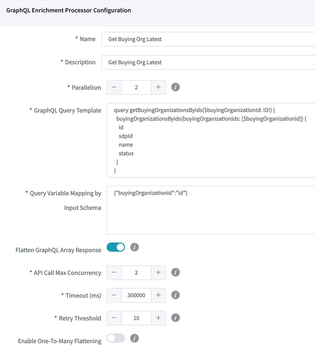
In the current Data Mesh Operational Reporting pipelines, the most commonly used intermediate processor is the GraphQL Enrichment Processor. It takes in the column value from CDC events coming from Source Connector as GraphQL query input, then submits a query to Studio Edge to enrich the data. With Studio Edge’s single data model, it centralizes data modeling efforts, which is highly leveraged by Studio UI Apps, Backend services and Search platforms. Enriching the data via Studio Edge helps us achieve consistent data modeling across the whole ecosystem for Operational Reporting.
Here is the example of GraphQL processor configuration, pipeline builder only need config the following fields to provision an enrichment processor:
GraphQL Enrichment Processor Configuration Example
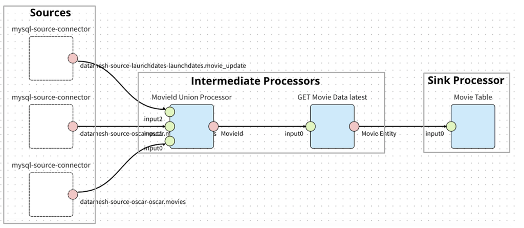
The image below is a sample Operational Reporting pipeline in the production environment to sink the Movie related data. Teams who want to move their data no longer need to learn and write customized Stream Processing jobs. Instead they just need to configure the pipeline topology in the UI while getting other features like schema evolution and secure data access out of the box.
Operational Reporting Pipeline Example
Iceberg Sink
Apache Iceberg is an open source table format for huge analytics datasets. Data Mesh leverages Iceberg tables as data warehouse sinks for downstream analytics use cases. Currently Iceberg sink is appended only. Views are built on top of the raw Iceberg tables to retrieve the latest record for every primary key based on the operational timestamp, which indicates when the record is produced in the sink. Current pipeline consumers are directly consuming Views instead of raw tables.
The compaction process is needed to optimize the performance of downstream queries on the business view as well as lower costs of S3 GET OBJECT operations. A daily process ranks the records by timestamp to generate a data frame of compacted records. Old data files are overwritten with a set of new data files that contain only the compacted data.
Data Quality
Data Mesh provides metrics and dashboards at both the processor and pipeline level for operational observability. Operational Reporting pipeline owners will get alerts if something goes wrong with their pipelines. We also have two types of auditing on the data tables generated from Data Mesh pipelines to guarantee data quality: end-to-end auditing and synthetic events.
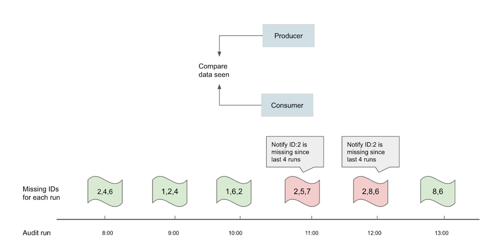
Most of the business views created on top of the Iceberg tables can tolerate a few minutes of latency. However, it is paramount that we validate the complete set of identifiers such as a list of movie ids across producers and consumers for higher overall confidence in the data transport layer of choice. For end-to-end audits, the objective is to run the audits hourly via Big data Platform Scheduler, which is a centralized and integrated tool provided by Netflix data platform for running workflows in an efficient, reliable and reproducible way. The audits check for equality (i.e. query results should be the same), the symmetric difference between two data sets should be empty across multiple runs, and the eventual consistency within the SLA. An hourly notification is sent when a set of primary keys consistently do not match between source of truth and target Data Mesh tables.
End to End (Black Box) Auditing Example
Synthetic events audits are artificially triggered change events to imitate common CUD operations of services. It is generating heartbeat signals at a constant frequency with the objective of using them as a baseline to verify the health of the pipeline regardless of traffic patterns or occasional silences.
Data Consumption
Our studio partners rely on data to make informed decisions and to collaborate during all the phases related to production. The Studio Tech Solutions team provides near real-time reports in some data tool of choice, which we call trackersto empower the decision making.
For the past few years, many of these trackers were powered by hand-curated SQL scripts and API calls being managed by CRON schedulers implemented in a Java Service called Lego. Lego was the main tool for the STS team, and at its peak, Lego managed 300+ trackers.
This strategy had its own set of challenges: being schema-less and treating every report column like a string not always worked out, the volatile reliance on direct RDS connections and rate limits from third party APIs would often make jobs fail. We had a set of “core views” which would be specifically tailored for reports, but this caused queries that just required a very small subset of fields to be slow and expensive due to the view doing a huge amount of joining and aggregation work before being able to retrieve that small subset.
Besides the issues, this worked fine when we didn’t have many trackers to maintain, but as we created more trackers to the point of having many hundreds, we started having issues around maintenance, awareness, knowledge sharing and standardization. New team members had a hard time getting onboard, figuring out which SQL powered which tracker was tough, the lack of standards made every SQL look different and having to update trackers as the data sources changed was a nightmare.
With this in mind, the Studio Tech Solutions focused efforts in building Genesis, a Semantic Data Layer that allows the team to map data points in Data Source Definitions defined as YAML files and then use those to generate the SQL needed for the trackers, based on a selection of fields, filters and formatters specified in an Input Definition file. Genesis takes care of joining, aggregating, formatting and filtering data based on what is available in the Data Source Definitions and specified by the user through the Input Definition being executed.
Genesis Data Source and Input definition example
Genesis is a stateless CLI written in Node.js that reads everything it needs from the file system based on the paths specified in the arguments. This allows us to hook Genesis into Jenkins Jobs, providing a GitOps and CI experience to maintain existing trackers, as well as create new trackers. We can simply change the data layer, trigger an empty pull request, review the changes and have all our trackers up to date with the data source changes.
As of the date of writing, Genesis powers 240+ trackers and is growing everyday, empowering thousands of partners in our studios globally to collaborate, annotate and share information using near-real-time data.
Git-based Tracker management workflow powered by Genesis and the Big Data Scheduler
The generated queries are then used in Workflow Definitions for multiple trackers. The Netflix Data Warehouse offers support for users to create data movement workflows that are managed through our Big Data Scheduler, powered by Titus.
We use the scheduler to execute our queries and move the results to a data tool, which often is a Google Sheet Tab, Airtable base or Tableau dashboard. The scheduler offers templated jobs for moving data from a Presto SQL output to these tools, making it easy to create and maintain hundreds of data movement workflows.
The diagram below summarizes the data consumption flow when building trackers:
Data Consumption Overview
As of July 2021, the Studio Tech Solutions team is finishing a migration from all the trackers built in Lego to use Genesis and the Data Portal. This strategy has increased the Studio Tech Solutions team performance and stability. Trackers are now easy for the team to create, review, change, monitor and discover.
Now and Future
In conclusion, our studio partners have a tracker available to them, populated with near real-time data and tailored to their needs. They can manipulate, annotate, and collaborate using a flexible tool they are familiar with.
Along the journey, we have learned that evolving data movement in complex domains could take multiple iterations and needs to be driven by the business impact. The great cross-functional partnership and collaboration among all data stakeholders is crucial to shape the ideal data product.
However, our story doesn’t end here. We still have a long journey ahead of us to fulfill the vision of such ideal data product, especially in areas such as:
Self-servicing data pipelines provisioning via configuration
Providing toolings for data discoverability, understandability, usage visibility and change management
Enabling data domain orientation and ownership/governance management
Bootstrapping trackers in our Studio ecosystem instead of third party tools. Along the same line as the point above, this would allow us to maintain high standards of data governance, lineage, and security.
Read-write reports and trackers using GraphQL mutations
These are some of the interesting areas that Netflix Studio is planning to invest in. We will have follow up blog posts on these topics in future. Please stay tuned!
Amazon MSK is a fully managed service that helps you build and run applications that use Apache Kafka to process streaming data. Apache Kafka is an open-source platform for building real-time streaming data pipelines and applications. With Amazon MSK, you can use native Apache Kafka APIs to populate data lakes. You can also stream changes to and from databases, and power machine learning and analytics applications.
Amazon MSK simplifies the setup, scaling, and management of clusters running Apache Kafka. MSK manages the provisioning, configuration, and maintenance of resources for a highly available Kafka clusters. It is fully compatible with Apache Kafka and supports familiar community-build tools such as MirrorMaker 2.0, Kafka Connect and Kafka streams.
Introduction
In the past few years, the volume of data that companies must ingest has increased significantly. Information comes from various sources, like transactional databases, system logs, SaaS platforms, mobile, and IoT devices. Businesses want to act as soon as the data arrives. This has resulted in increased adoption of scalable real-time streaming solutions. These solutions scale horizontally to provide the needed throughput to process data in real time, with milliseconds of latency. Customers have adopted Amazon MSK as a top choice of streaming platforms. Amazon MSK gives you the flexibility to retain topic data for longer term (default 7 days). This supports replay, analytics, and machine learning based use cases. When IT and business systems are producing and processing terabytes of data per hour, it can become expensive to store, manage, and retrieve data. This has led to legacy data archival processes moving towards cheaper, reliable, and long-term storage solutions like Amazon Simple Storage Service (S3).
Following are some of the benefits of archiving Amazon MSK topic data to Amazon S3:
Reduced Cost – You only must retain the data in the cluster based on your Recovery Point Objective (RPO). Any historical data can be archived in Amazon S3 and replayed if necessary.
Integration with Enterprise Data Lake – Since your data is available in S3, you can now integrate with other data analytics services like Amazon EMR, AWS Glue, Amazon Athena, to run data aggregation and analytics. For example, you can build reports to visualize month over month changes.
Optimize Machine Learning Workloads – Machine learning applications will be able to train new models and improve predictions using historical streams of data available in Amazon S3. This also enables better integration with Amazon Machine Learning services.
Compliance – Long-term data archival for regulatory and security compliance.
Backloading data to other systems – Ability to rebuild data into other application environments such as pre-prod, testing, and more.
There are many benefits to using Amazon S3 as long-term storage for Amazon MSK topics. Let’s dive deeper into the recommended architecture for this pattern. We will present an architecture to back up Amazon MSK topics to Amazon S3 in real time. In addition, we’ll demonstrate some of the use cases previously mentioned.
Architecture
The diagram following illustrates the architecture for building a real-time archival pipeline to archive Amazon MSK topics to S3. This architecture uses an AWS Lambda function to process records from your Amazon MSK cluster when the cluster is configured as an event source. As a consumer, you don’t need to worry about infrastructure management or scaling with Lambda. You only pay for what you consume, so you don’t pay for over-provisioned infrastructure.
To create an event source mapping, you can add your Amazon MSK cluster in a Lambda function trigger. The Lambda service internally polls for new records or messages from the event source, and then synchronously invokes the target Lambda function. Lambda reads the messages in batches from one or more partitions and provides these to your function as an event payload. The function then processes records, and sends the payload to an Amazon Kinesis Data Firehose delivery stream. We use Kinesis Data Firehose delivery stream because it can natively batch, compress, transform, and encrypt your events before loading to S3.
In this architecture, Kinesis Data Firehose delivers the records received from Lambda in Gzip file to Amazon S3. These files are partitioned in hive style format by Kinesis Data Firehose:
data/year = yyyy/month = MM/day = dd/hour = HH
Figure 1. Archival Architecture
Let’s review some of the possible solutions that can be built on this archived data.
Integration with Enterprise Data Lake
The architecture diagram following shows how you can integrate the archived data in Amazon S3 with your Enterprise Data Lake. Since the data files are prefixed in hive style format, you can partition and store the Data Catalog in AWS Glue. With partitioning in place, you can perform optimizations like partition pruning, which enables predicate pushdown for improved performance of your analytics queries. You can also use AWS Data Analytics services like Amazon EMR and AWS Glue for batch analytics. Amazon Athena can be used to run serverless SQL-like interactive queries on visualization and data.
Data currently gets stored in JSON files. Following are some of the services/tools that can be integrated with your archive for reporting, analytics, visualization, and machine learning requirements.
Figure 2. Analytics Architecture
Cloning data into other application environments
There are use cases where you would want to use this data to clone other application environments using this archive.
These clusters could be used for testing or debugging purposes. You could decide to use only a subset of your data from the archive. Let’s say you want to debug an issue beyond the configured retention period, but not replicate all the data to your testing environment. With archived data in S3, you can build downstream jobs to filter data that can be loaded into a new Amazon MSK cluster. The following diagram highlights this pattern:
Figure 3. Replay Architecture
Ready for a Test Drive
To help you get started, we would like to introduce an AWS Solution: AWS Streaming Data Solution for Amazon MSK (scroll down and see Option 3 tab). There is a single-click AWS CloudFormation template, which can assist you in quickly provisioning resources. This will get your real-time archival pipeline for Amazon MSK up and running quickly. This solution shortens your development time by removing or reducing the need for you to:
Model and provision resources using AWS CloudFormation
Manually implement streaming data best practices in AWS
This solution is data and logic agnostic, enabling you to start with boilerplate code and start customizing quickly. After deployment, use this solution’s monitoring capabilities to transition easily to production.
Conclusion
In this post, we explained the architecture to build a scalable, highly available real-time archival of Amazon MSK topics to long term storage in Amazon S3. The architecture was built using Amazon MSK, AWS Lambda, Amazon Kinesis Data Firehose, and Amazon S3. The architecture also illustrates how you can integrate your Amazon MSK streaming data in S3 with your Enterprise Data Lake.
As businesses race to digitally transform, the challenge is to cope with the amount of data, and the value of that data diminishes over time. The challenge is to analyze, learn, and infer from real-time data to predict future states, as well as to detect anomalies and get accurate results. In this blog post, we’ll explain the architecture for a solution that can achieve real-time inference on streaming data. We’ll also cover the integration of Amazon Kinesis Data Analytics (KDA) with Apache Flink to asynchronously invoke any underlying services (or databases).
Managed real-time in-stream data inference is quite a mouthful; let’s break it up:
In-stream data refers to the capability of processing a data stream that collects, processes, and analyzes data.
Real-time inference refers to the ability to use data from the feed to project future state for the underlying data.
Consider a streaming application that captures credit card transactions along with the other parameters (such as source IP to capture the geographic details of the transaction as well as the amount). This data can then be used to be used to infer fraudulent transactions instantaneously. Compare that to a traditional batch-oriented approach that identifies fraudulent transactions at the end of every business day and generates a report when it’s too late, after bad actors have already committed fraud.
Architecture overview
In this post, we discuss how you can use Amazon Kinesis Data Analytics for Apache Flink (KDA), Amazon SageMaker, Apache Flink, and Amazon API Gateway to address the challenges such as real-time fraud detection on a stream of credit card transaction data. We explore how to build a managed, reliable, scalable, and highly available streaming architecture based on managed services that substantially reduce the operational overhead compared to a self-managed environment. Our particular focus is on how to prepare and run Flink applications with KDA for Apache Flink applications.
The following diagram illustrates this architecture:
In above architecture, data is ingested in AWS Kinesis Data Streams (KDS) using Amazon Kinesis Producer Library (KPL), and you can use any ingestion patterns supported by KDS. KDS then streams the data to an Apache Flink-based KDA application. KDA manages the required infrastructure for Flink, scales the application in response to changing traffic patterns, and automatically recovers from underlying failures. The Flink application is configured to call an API Gateway endpoint using Asynchronous I/O. Residing behind the API Gateway is an AWS SageMaker endpoint, but any endpoints can be used based on your data enrichment needs. Flink distributes the data across one or more stream partitions, and user-defined operators can transform the data stream.
Let’s talk about some of the key pieces of this architecture.
What is Apache Flink?
Apache Flink is an open source distributed processing framework that is tailored to stateful computations over unbounded and bounded datasets. The architecture uses KDA with Apache Flink to run in-stream analytics and uses Asynchronous I/O operator to interact with external systems.
KDA and Apache Flink
KDA for Apache Flink is a fully managed AWS service that enables you to use an Apache Flink application to process streaming data. With KDA for Apache Flink, you can use Java or Scala to process and analyze streaming data. The service enables you to author and run code against streaming sources. KDA provides the underlying infrastructure for your Flink applications. It handles core capabilities like provisioning compute resources, parallel computation, automatic scaling, and application backups (implemented as checkpoints and snapshots).
Flink Asynchronous I/O Operator
Flink’s Asynchronous I/O operator allows you to use asynchronous request clients for external systems to enrich stream events or perform computation. Asynchronous interaction with the external system means that a single parallel function instance can handle multiple requests and receive the responses concurrently. In most cases this leads to higher streaming throughput. Asynchronous I/O API integrates well with data streams, and handles order, event time, fault tolerance, etc. You can configure this operator to call external sources like databases and APIs. The architecture pattern explained in this post is configured to call API Gateway integrated with SageMaker endpoints.
Please refer code at kda-flink-ml, a sample Flink application with implementation of Asynchronous I/O operator to call an external Sagemaker endpoint via API Gateway. Below is the snippet of code of StreamingJob.java from sample Flink application.
The operator code above requires following inputs:
An input data stream
An implementation of AsyncFunction that dispatches the requests to the external system
Timeout, which defines how long an asynchronous request may take before it considered failed
Capacity, which defines how many asynchronous requests may be in progress at the same time
How Amazon SageMaker fits into this puzzle
In our architecture we are proposing a SageMaker endpoint for inferencing that is invoked via API Gateway, which can detect fraudulent transactions.
Amazon SageMaker is a fully managed service that provides every developer and data scientist with the ability to build, train, and deploy machine learning (ML) models quickly. SageMaker removes the heavy lifting from each step of the machine learning process to make it easier to build and develop high quality models. You can use these trained models in an ingestion pipeline to make real-time inferences.
You can set up persistent endpoints to get predictions from your models that are deployed on SageMaker hosting services. For an overview on deploying a single model or multiple models with SageMaker hosting services, see Deploy a Model on SageMaker Hosting Services.
Ready for a test drive
To help you get started, we would like to introduce an AWS Solution: AWS Streaming Data Solution for Amazon Kinesis (Option 4) that is available as a single-click cloud formation template to assist you in quickly provisioning resources to get your real-time in-stream inference pipeline up and running in a few minutes. In this solution we leverage AWS Lambda, but that can be switched with a SageMaker endpoint to achieve the architecture discussed earlier in this post. You can also leverage the pre-built AWS Solutions Construct, which implements an Amazon API Gateway connected to an Amazon SageMaker endpoint pattern that can replace AWS Lambda in the below solution. See the implementation guide for this solution.
The following diagram illustrates the architecture for the solution:
Conclusion
In this post we explained the architecture to build a managed, reliable, scalable, and highly available application that is capable of real-time inferencing on a data stream. The architecture was built using KDS, KDA for Apache Flink, Apache Flink, and Amazon SageMaker. The architecture also illustrates how you can use managed services so that you don’t need to spend time provisioning, configuring, and managing the underlying infrastructure. Instead, you can spend your time creating insights and inference from your data.
We also talked about the AWS Streaming Data Solution for Amazon Kinesis, which is an AWS vetted solution that provides implementations for applications you can automatically deploy directly into your AWS account. The solution automatically configures the AWS services necessary to easily capture, store, process, and infer from streaming data.
The collective thoughts of the interwebz
Manage Consent
To provide the best experiences, we use technologies like cookies to store and/or access device information. Consenting to these technologies will allow us to process data such as browsing behavior or unique IDs on this site. Not consenting or withdrawing consent, may adversely affect certain features and functions.
Functional
Always active
The technical storage or access is strictly necessary for the legitimate purpose of enabling the use of a specific service explicitly requested by the subscriber or user, or for the sole purpose of carrying out the transmission of a communication over an electronic communications network.
Preferences
The technical storage or access is necessary for the legitimate purpose of storing preferences that are not requested by the subscriber or user.
Statistics
The technical storage or access that is used exclusively for statistical purposes.The technical storage or access that is used exclusively for anonymous statistical purposes. Without a subpoena, voluntary compliance on the part of your Internet Service Provider, or additional records from a third party, information stored or retrieved for this purpose alone cannot usually be used to identify you.
Marketing
The technical storage or access is required to create user profiles to send advertising, or to track the user on a website or across several websites for similar marketing purposes.