Анти-примери в озеленяването – сградата на Блъсков в Дианабад

Post Syndicated from Боян Юруков original https://yurukov.net/blog/2026/ozelenyavane-5/

Поредният пример от поредицата ми за нередности в задължителното озеленяване е тази на Блъсков в Дианабад. За разлика от предишният пример, който е буквално отсреща на улицата, тази сграда е готова от години. Аналогично дава ярки примери за пълно незачитане на нормативните разпоредби, нарушения при приемането на обектите и какво неизменно следва веднага като мине акт 16. Разликата с описаното в предишните статии може би е, че там инвеститорите развяват претенции за лукс, качество и най-вече всеобхватна зеленина и екологичност на строежите. Твърдения в рязък контраст с наблюдаваното както в проектната документация, така и на място в строежите. Блъсков и близките му замесени в този строеж поне не се крият какви са.

Както на много други строежи, озеленяването е навярно най-малкия проблем. Този конкретно стана злощастно известен със схемата, в която Фандъкова направи заменка на имот на един от синовете на Блъсков с това място, което трябваше да стане разширение на детската градина. Повече за това и протестите ще намерите в Mediapool и Капитал. Бях на протестите тогава и станах свидетел колко нагло се държа Блъсков и колко лъга. В крайна сметка схемата му успя и прибра значителна печалба с подаръка от същото икономическо мнозинство, което държи и сега СОС.

Част от тази печалба беше възможна именно, защото приложи масовата схема да застрои сградата значително повече от разрешеното. Формално кинтът е спазен, но това е възможно единствено, защото са спестили значително от озеленяването. Преди дни получих от ДНСК протокола на приемателната комисия и ще споделя какви са изводите им. Първо нека разгледаме какво се вижда на място.

Сегашно състояние

Сградата е върху два парцела – 68134.803.3950 и 68134.803.3951. На практика е една и съща и е свързана. На първата снимка виждате южната страна, където с вкопани няколко саксии с храсчета, а останалото, което би следвало да се е зелена площ, винаги е било запълнено с декоративни камъни и трици. Под него на съвсем плитко е бетон та дори трева не би оцеляла.

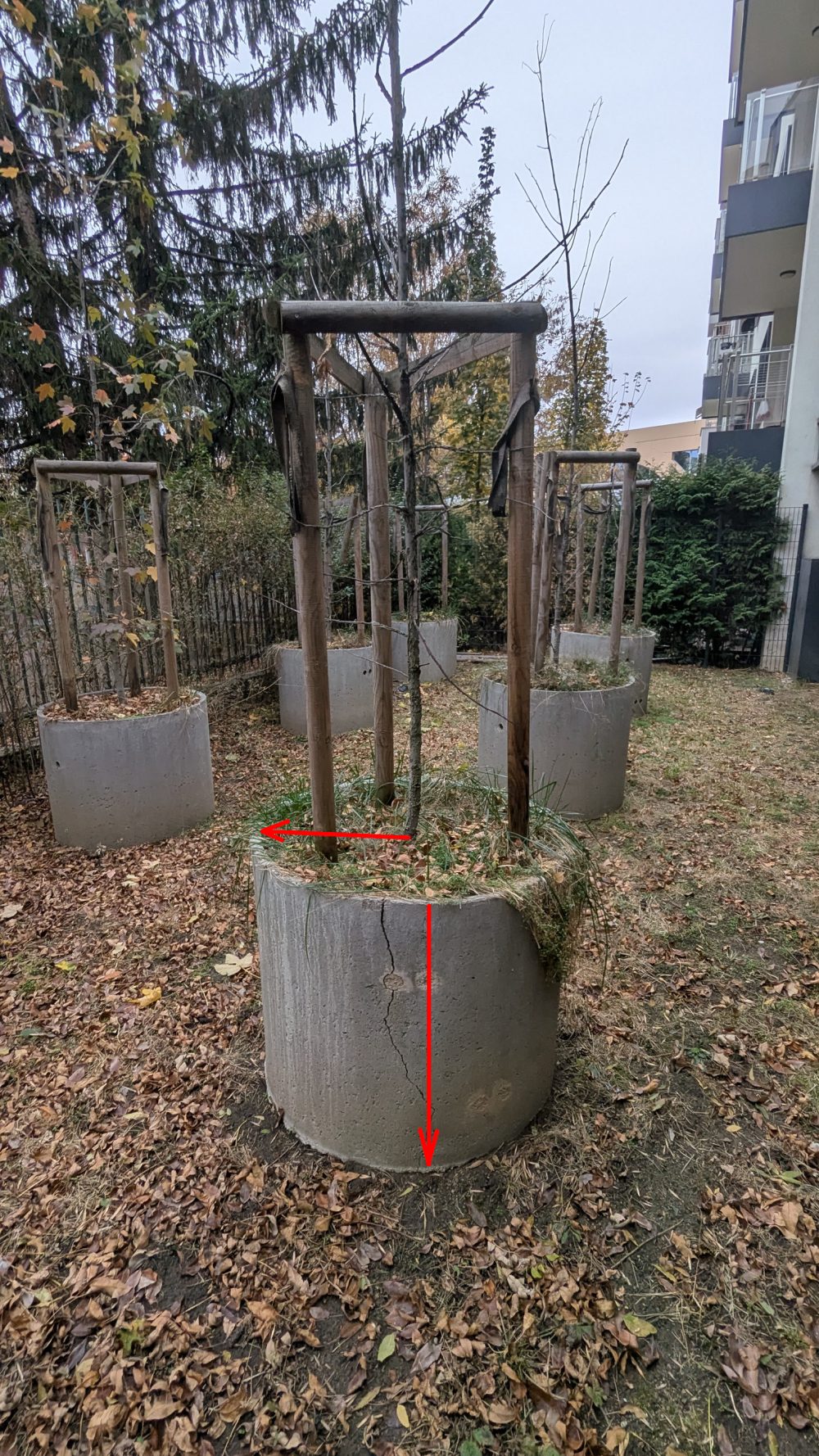
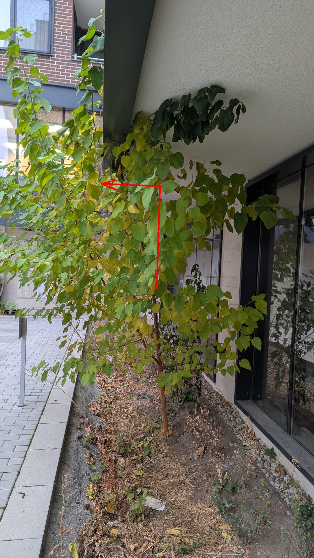
На втората снимка виждате другата страна на южната част където се вижда първото дърво. Както всички останали, които ще видите, то е в „кашпа“ представляваща бетонен елемент за тръба с диаметър и височина 80 см. За почти четири години дървото е с дебелина от два сантиметра. Причината е, че няма дори теоретична възможност да порасне. Изискванията за почвен слой са минимум 120 см., а при кашпа трябва да има поне един кубичен метър почва. Всяка от тези тръби побира най-много 0.4 кубични метра. С други думи нито тази, нито която и от другите подобни дървета не отговаря на нормативните изисквания нито сега, нито когато е била завършена сградата. До него се виждат още едно декоративно дърво, което е практически под стряхата и също не отговаря на изискванията.

На третата снимка се вижда алеята между сградата и детската градина. Има няколко дървета останали от преди строежа. Преди строежа отсякоха много дървета в имота – най-вероятно без разрешение. Зад няколкото оцелели на снимки четири до седем се виждат седем дървета в кашпи подобни на предишната и още три дървета засадени в земята. Всички са останали тънки вейки след четири години в земята. Нито едно от седемте кашпи не отговаря на изискванията. В протокола на приемателната комисия твърдят, че някои от дърветата са с 140 см. почвен слой. Предвид видяното на място и схемите за подземните гаражи това не изглежда да е вярно.

На осма снимка се вижда малка градинка, с която според протокола са заменили зелен хълм в плана за озеленяване. Тя е изцяло под навес на фасадата, няма дървета и храсти, но поне явно някой се занимава да я поддържа. Това личи и на девета снимка, която направих две седмици по-късно. Вижда се, че са засадили нови цветя и махнали други растения. Причината вероятно е, че лехата е крайно недостатъчна, за да оцелеят храсти и по-сериозна растителност.

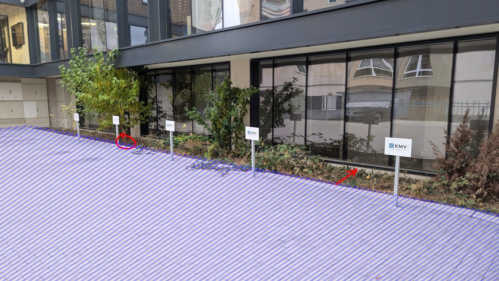
Не това може да се каже за вътрешния двор. На снимка десет се вижда зелена площ, която е почти изцяло покрита с плочи или техника. Почвеният слой е под 5 см., което значи, че не може да се зачита към индекса за задължителното озеленяване. В синьо на същата снимка виждате паркоместа зад нея, които според акт 16 е зелена площ на ивици с дървета. По-добре се вижда мястото на снимка единадесет. Същото важи за снимки 12 и 13 – в синьо може да си мислите, че виждате паркоместа върху паваж, но всъщност е зелена площ на ивици, отново с дървета засадени между тях.

Зад паркоместата до фасадата виждаме малкото оцеляла зеленина. Виждаме я на снимка 14. Тя е изцяло под стреха и има 1-2 дървета, едно от които буквално удря в тавана. Изискването е да е на поне метър от навеса, но навън, не навътре. Виждаме, че и почва почти няма в лехата, което ни позволява да наблюдаваме чест проблем – половината всъщност е бетонирана. Когато се мерят подобни лехи по размерите до бордюра се пропуска, че буквално сантиметри надолу е бетон под ъгъл, за да държи на място въпросния бордюр. Така често в поне 30% от площта зелените площи не може да говорим за нужната дълбочина на почвения слой. Това обаче не е регламентирано в наредбата. Всъщност, дори регламентираните неща в нея не се спазват масово, което показвам с тази поредица.

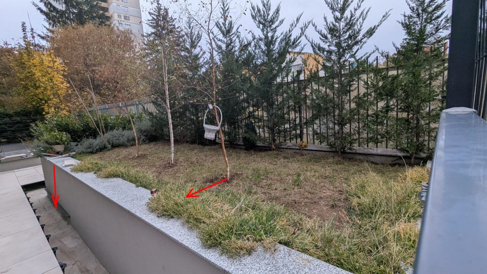
Снимка 15 показва малка леха от северната страна. Там са заболи един клен, който бере душа. Почвеният слой е колкото саксия на балкон. На 16-та снимка се виждат още паркоместа, които се водят за озеленяване. Всъщност, маркираното в синьо е било леха с предполагаемо дърво, но веднага е бетонирано, защото явно е пречело. На последната снимка 17 се вижда издигната леха, която се води за „вертикално озеленяване“ според проекта. Почвеният слой, отстоянията от бордюра и всичко не отговарят на изискванията. Затова и онова, което се води за дървета е изсъхнало.

Промени през времето

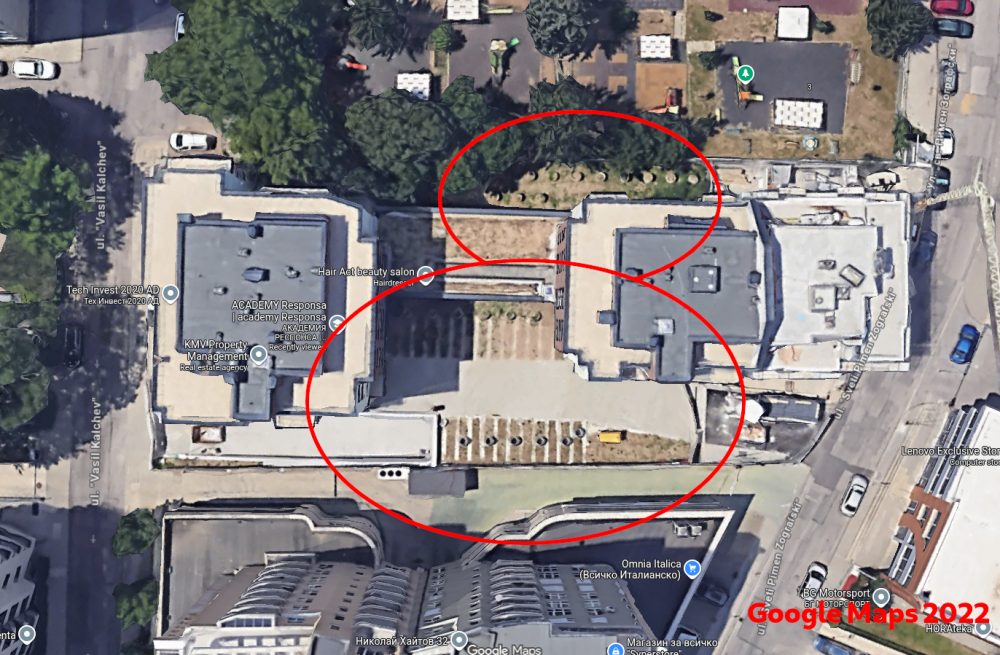
Както видяхме при Диамант 2 на Артекс, зелените площи стават паркоместа веднага след като мине приемателната комисия. На снимката долу виждате сателитна снимка от Google Maps на обсъжданата сграда докато още се строеше през 2022 г. Виждат се зелените площи на лехи където сега има бетон и паркоместа. Същите се виждат горе в снимките отбелязани в синьо. Виждат се храсти, но не и дървета. В горната част се виждат 12 „кашпи“ и предполагаемо дървета, а не 7 както сега. На този етап сградата се довършваше и подготвяше за проверка.
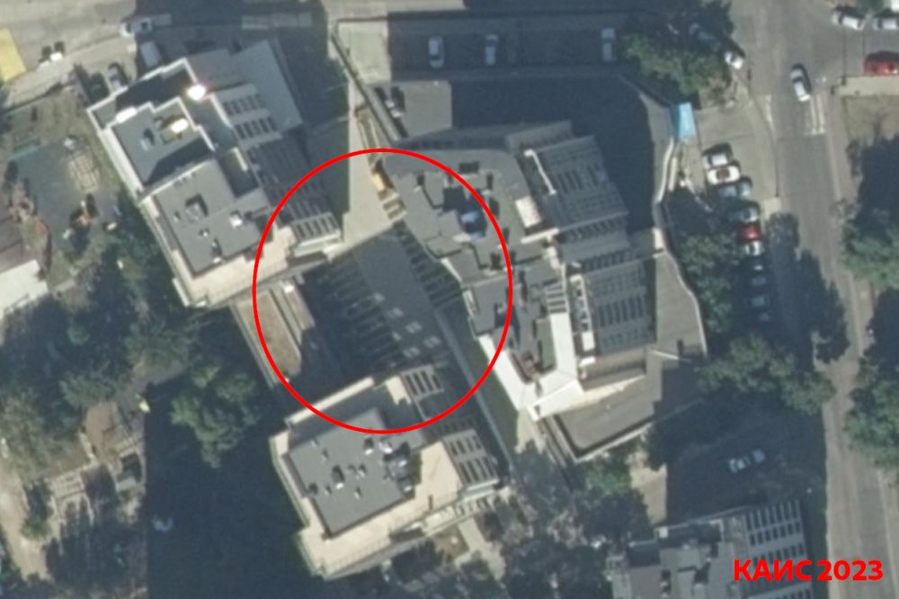
Следващата снимка е от последните сателитни данни на КАИС. МРРБ се похвалиха с тях първо твърдейки, че са от 2026, но след критиката ми се поправиха и стана ясно, че София е заснета през лятото на 2023 г. Това значи, че лехите са оцелели около шест месеца. Все още не се виждат дървета където сега има паркоместа и където акт 16 настоява, че са били някак открити.
В iSofMap имаме снимки от 2024 и там вече се вижда, че лехите са бетонирани изцяло и имотът е вече в сегашното състояние.
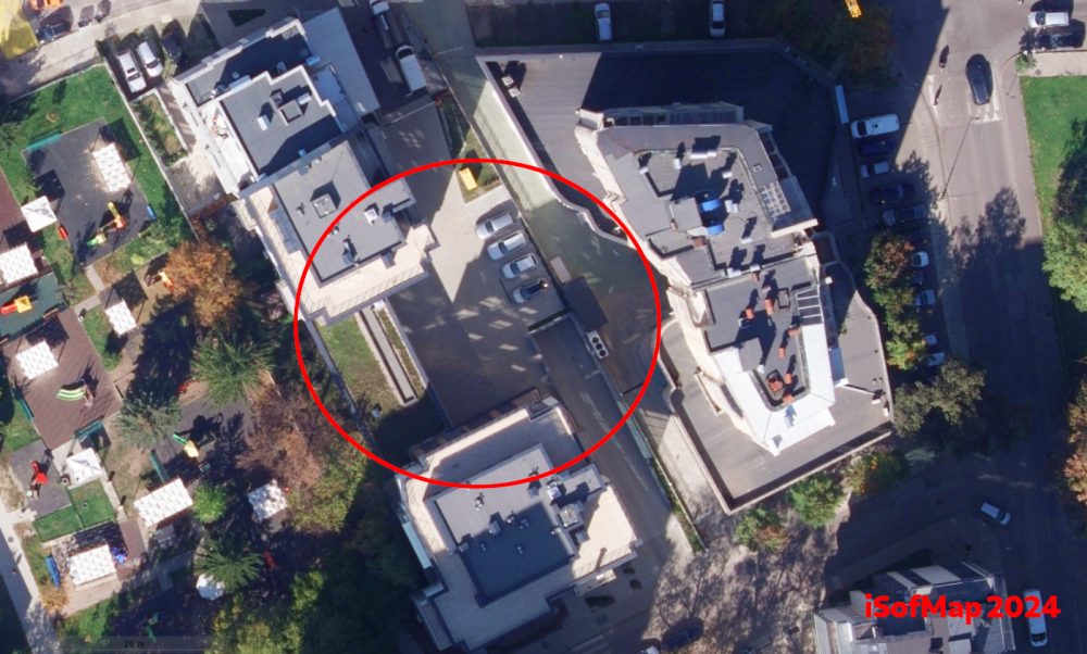
Сателитните снимки показват, че е имало промени в озеленяването между края на 2022 г. и 2024 г. Отделно снимките от лятото на 2023 г. и тези преди това показват, че никога не е имало дървета в лехите между или под паркоместата. Бетонната плоча над гаражите прави най-малкото невъзможно това.

Какво казва акт 16?

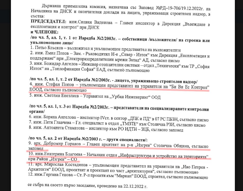
На 22 декември 2022 има заседание на приемателна комисия назначена със заповед на ДНСК три дни по-рано – РД-19-706/19.12.2022. Още на следващия ден – последен преди коледните празници – е извадено разрешение за ползване СТ-05-714/23.12.2022 за основната сграда. Това показва изключителна експедитивност за придвижване на документи и строеж видимо пълни с нарушения. Шест месеца по-късно има вече разрешение и за малката част – СТ-05-310/21.06.2023. Първото още не е достъпно сканирано, но второто ще намерите на страницата на ДНСК.

Получих протокола от приемателната комисия на голямата сградата след запитване по ЗДОИ до ДНСК (и споменаване на двете дела за идентичен документ, които спечелих). В него се забелязват няколко интересни факта. Първо, според декларираното в протокола зелените площи са изпълнени според всички изисквания, между паркоместата има бетонни пръстени и засети дървета. Твърди се че там почвения слой достига 140 см.
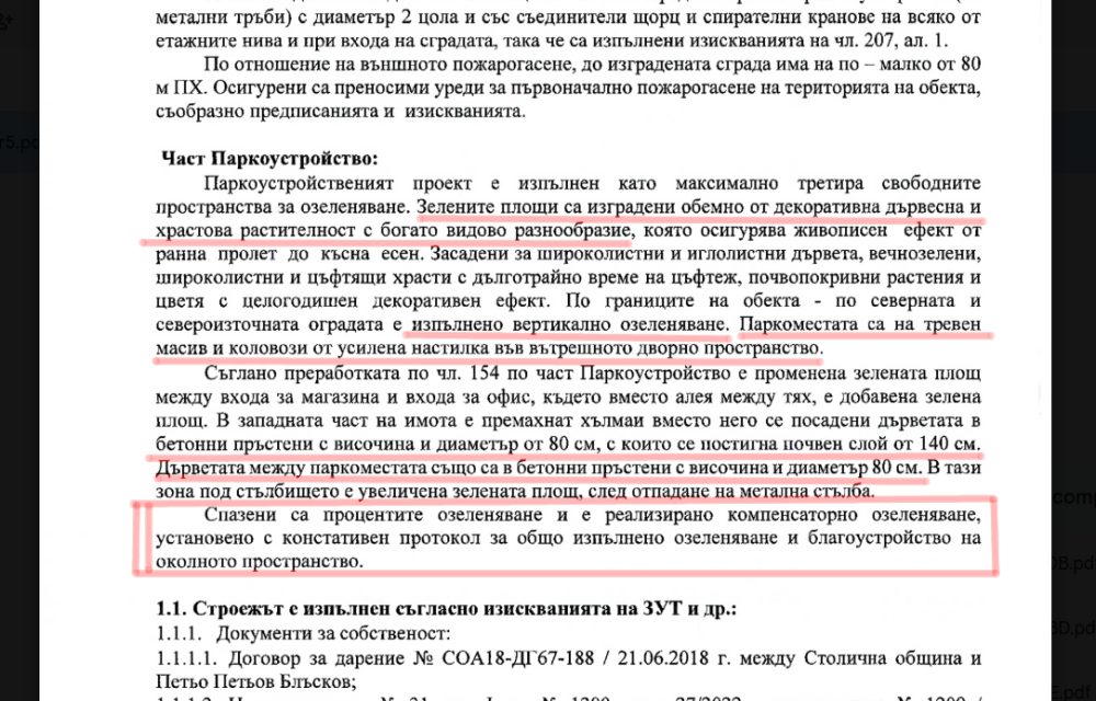
Изброеното е не само невярно, но и невъзможно. При паркоместата има бетонна плоча на сантиметри под тогавашните лехи и сегашните павета. Най-фрапантното е, че в протокола се описват въпросните бетонни пръстени с височина и диаметър 80 см. Изискването през 2022-ра също както сега е дърветата в кашпи да имат поне един кубичен метър почва. Така описани бетонните пръстени осигуряват 0.4 кубични метра. Дори да беше вярно това с дълбочината от 1.4 метра, това прави 0.7 кубика.

Това означава не само, че дърветата не могат да се развиват и ще умрат, но и че не може да се причисляват към изисканията за озеленяване според наредбата на Столична община. Доколкото в протокола са споменати промени спрямо планът за паркоустройство, от описаното и видяното на място става ясно, че изначално е било заложено бутафорно озеленяване с цел бетониране на паркоместата, липса на достатъчен почвен слой, никакъв шанс зеленината да оцелее или да е изпълнена заложената в изискванията цел.

Такова мнение може да си направим от думите на комисията и видяното на място. Противното може да се докаже единствено от архитектурните планове за конструкцията и паркоустройството. В протоколът е споменат архитектът отговорен за последното. По една странна и откровено лобистка дефиниция на закона за авторското право не мога да публикувам тези части от строителните книжа. Затова ще поискам да бъдат публикувани от арх. Василева или да даде разрешение да го сторя. Ако се окаже, че са изрядни и сградата е построена грешно, то значи протоколът лъже по различен начин и други хора следва да носят отговорност.
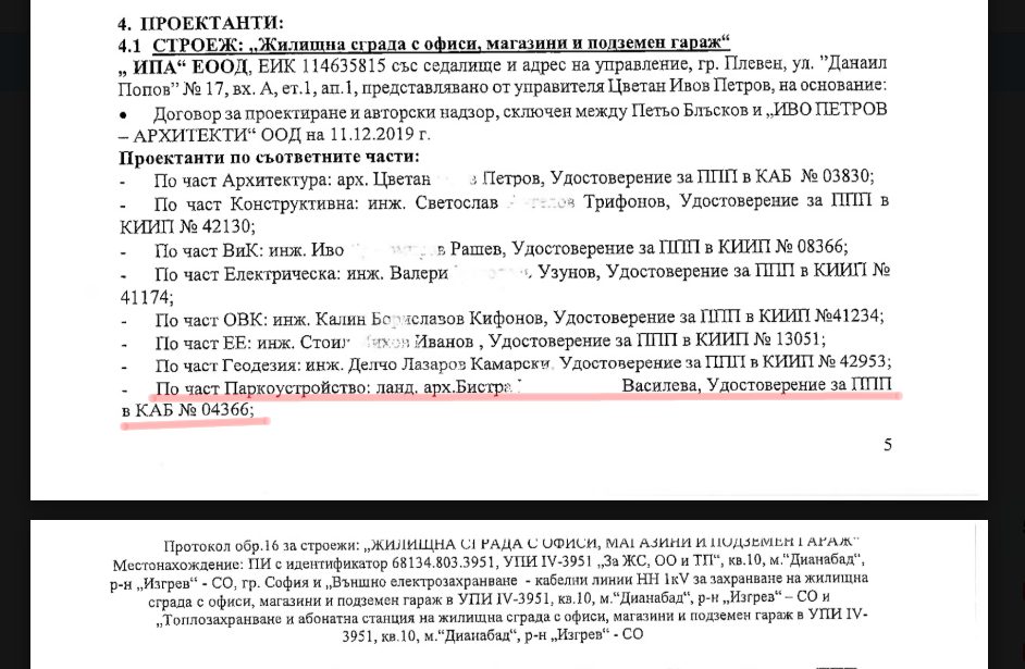
Независимо от това, вижда се ясно на място, както и от сателитни снимки малко и преди комисията, че дървета е нямало, почвеният слой не се различава от сегашния и не отговаря на изискванията. Дори от самия протокол разбираме, че кашпите не е следвало да се приемат. Конкретно за приемане на озеленяването отговаря районната община. В протокола пише, че от район Изгрев за това се е подписал арх. Горанов. Т.е. на база описаното сградата никога не е следвало да бъде пускана в експлоатация най-малкото заради озеленяването и този подпис неправомерно е позволил това.
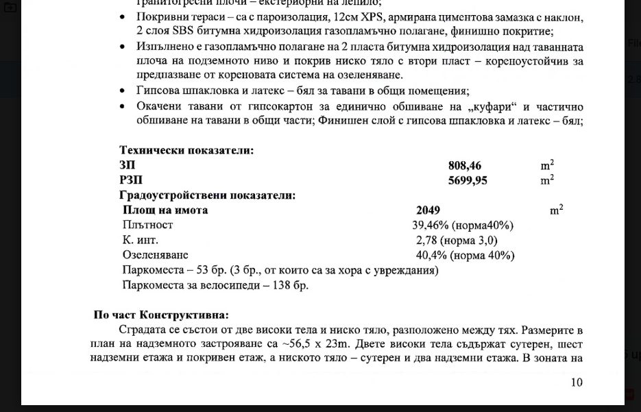
Този протокол се отнася до имот 68134.803.3951 и първото разрешение за ползване. Описват параметрите на застрояване. Според тях са постигнали поне 40% озеленяване. На място премерих не повече от 25% включвайки зеления покрив. Включвайки бетонираните паркоместа трудно би минало 35%. Тук следва да се вземе предвид, че повечето от тези зелени площи не следва въобще да се включат в сметката заради малкия почвен слой, липсата на отстояния и други несъответствия.

От същата страница научаваме, че само в голямата част от сградата са предвидили 53 паркоместа и още 138 за колелета. Доколкото е трудно да се прецени колко коли са побрали в подземните гаражи без да се влезе там, убеден съм, че няма място за дори 20 колелета. Според изискванията, трябва да имат поне 79.
Какво следва?

Разрешенията за ползване са съответно от декември 2022 и юни 2023. Това значи, че районната администрация е длъжна да проверява дали озеленяването отговаря на тогавашните изисквания до декември 2027 и юни 2028. При аналогични сигнали за сграда на Артекс районният кмет на Изгрев години наред настояваше, че не вижда нередности, после като откри такива отказа да провери цялата сграда, а като все пак получих плана за озеленяване и описах несъответствията, отсече, че то хубаво, ама тъкмо бил изтекъл срокът и вече не можело нищо да направи.

В този случай не очаквам нещо по-различно. Всъщност, още няма действия по сигналите ми за хотела на 4-ти км. където освен незаконния видео билборд се оказа, че поне половината задължително озеленяване липсва. Очаквам същите проблеми когато ДНСК разреши ползване на новата сграда на Артекс и тази на Тинтява 80 въпреки, че по аналогични на горния пример причини озеленяването никога не може да отговаря на изискванията с такава интензивност на застрояване и къде е излят бетонът. Може да прочетете повече защо е важно озеленяването и за тази серия от статии.

Това не значи, че няма да предам откритото като сигнал до районната община. Най-малкото, за да се документира отказът им и/или липсата на действие. Истината тук е, че процесът на контрол е счупен, а изискванията са крайно недостатъчни и меко дефинирани. Знам, че според някои архитекти и всички инвеститори са дори прекомерни, но в действителност не са достатъчни, за да осигурят заложените в тях целите. Отделно дори това, което е ясно разписано не се спазва, отчасти заради оставените вратички.

Затова следва да се разширят значително като параметри – почвен слой, отстояния и да се прецизират като изисквания. Следва да се промени ЗУТ и да се махне ограничението от 5 години за последващи проверки и промяната да важи за вече построени сгради независимо кога са били завършени. С последното няма да се нарушава правата на собствениците, тъй като никъде в закона няма презумпция, че след 5 години (или както е по-често – 5 дни) могат да разкарат всички кашпи и да бетонират всички лехи. Срокът ограничава възможността за контрол, а не дава имплицитно разрешение за неразрешени по архитектурен план промени.

Още по-важно е да се документират всички дървета в градската среда и приоритетно в тези регистри да влизат дърветата установени при приемане на строежи, компенсиращото залесяване и съществуващите дървета в частни имоти. Следва да се облекчи и автоматизира режимът на подаване на сигнали и налагане на глоби на база свидетелски показания с цел намаление на административната тежест и покриване на хилядите строежи никнещи всяка година. Трябва да започне да се прилага европейският регламент диктуващ, че дърветата и зелените площи в градска среда не може да намаляват. Това трябва да стане чрез отказ от премахване на дървета за нови строежи и значително увеличаване на изискванията за компенсиращо залесяване в рамките на самия имот.

Не на последно място, трябва да въведем принципа на виртуалното дърво – ако някой отсече неправомерно или умъртви дърво, това трябва да се документира и точното местоположение да се отбележи запазено за бъдещо такова в следващите поне 15 години. Често извършителят остава неизвестен въпреки хилещите се наблизо ръководители на бъдещия строеж. Местната администрация даже не се занимава да документира или глобява. За тази цел не трябва да има значение чия е земята и кой е извършителят – имало ли е дърво, мястото трябва да остане незастроено и в поне радиус от 4 метра около или под него не следва да има бетон, фасади или други конструкции. Мястото да бъде определено за залесяване от общината и да се посади същият или аналогичен вид дърво. Промени на тези обстоятелства да стават единствено с решение на общинския съвет.

Често обаче дърветата не са в регистър и се изсичат през почивните дни, премахват се пъновете и се маха всякаква следа. При липса на преки доказателства или документация, трябва да се приемат сведения от трима живущи в района като достатъчно доказателство. Т.е. да може трима съседи да се подпишат носейки отговорност за думите си, че на това място до скоро е имало дърво. Тогава да се определя това място като „виртуално дърво“ с цел защита срещу бъдещо бетониране, за да се засади ново и да получи шанс да порасне до размерите на отсеченото. Щом трима свидетели са достатъчни за възстановяване на земя чрез реституция заради спомени, че някой я е бил орал преди десетилетия, то същият принцип не пречи да се приложи за едно дърво и събития случили се преди дни.

Това е единственият шанс да се вдигне реалната цена на незаконно унищожено дърво. Глобите са недостатъчни и не се налагат. Когато премахнато дърво поставя под риск цял инвестиционен проект, може би ще започне да се мисли повече за зеленината в градската среда също от страна на строителите. Разбира се, очаквам веднага да креснат с аргументи за цената на жилищата, които отдавна бяха оборени.

Тази и предишните мерки следва да се приложат не само в София, но и за цялата страна. Аналогични проблеми има във всички градове и всеки от нас може да даде примери. Тези, с които илюстрирам казуса в тази поредица, срещам всеки ден пътувайки из града. Някои са само на хвърлей камък един от друг и демонстрират фрапантни нарушения сам по себе си.

А за тази конкретно сграда ще видим. Никой няма надежда, че в следващите 12 до 18 месеца местната администрация ще започне да взима мерки дори в рамките на сегашните си правомощия. Доколкото отчасти е несъмнено въпрос на липсващ административен капацитет и скъпа съдебна процедура, в случая е въпрос на липса на желание от страна на районната администрация отговорна за всички сгради описани до тук. Документите показват, че може да става въпрос и за съучастие. Скоро ще разкажа за протоколите за сградата на Артекс и хотелът на Тиков и ще се разбере дали същото ще изскочи и там.

AMD Launches EPYC Embedded 9006: Venice Gets an Early Start in Embedded

Post Syndicated from Ryan Smith original https://www.servethehome.com/amd-launches-epyc-embedded-9006-venice-gets-an-early-start-in-embedded/

With its new Zen 6 “Venice” silicon in hand, AMD has launched its next-generation EPYC Embedded 9006 platform for the embedded market, aiming to bring the performance benefits of the new platform to the long term stability-focused market segment

The post AMD Launches EPYC Embedded 9006: Venice Gets an Early Start in Embedded appeared first on ServeTheHome.

Upcoming Speaking Engagements

Post Syndicated from Bruce Schneier original https://www.schneier.com/blog/archives/2026/11/upcoming-speaking-engagements-62.html

This is a current list of where and when I am scheduled to speak:

  • I’m speaking at the Catalyst Summit in Brampton, Ontario, Canada, on Wednesday, November 18, 2026.
  • I’m speaking at QT Qonference 2026 in Toronto, Ontario, Canada, on Thursday, November 19, 2026.

The list is maintained on this page.

Седмицата (9–14 ноември)

Post Syndicated from Светла Енчева original https://www.toest.bg/sedmitsata-9-14-noemvri/

Седмицата (9–14 ноември)

Ако четете този бюлетин, светът не е свършил на вчерашния 13 ноември, петък, както са предвидили учени през 1960 г. На 10 ноември, точно 37 години след падането на тоталитарния режим обаче, светът свърши за 12 души, пътуващи по магистрала „Тракия“ в посока Бургас.

И нека не се оставяме да ни приспят с оправданието, че мъглата е виновна. Това не е мъглата от разказа на Борис Виан, а най-нормална есенна мъгла, за каквато пътищата в България би трябвало да са подготвени. Тя може да доведе до фатални последици само в комбинация с други фактори – некачествена пътна настилка, шофьори, които карат като на рали, липса на светлинни табели, липса на адекватен контрол…

Но трагедията показа също, че в България гражданското общество може да бъде активно. Поне в някои случаи. На призивите за кръводаряване се отзоваха стотици. Не забелязах обаче редом с призивите да се разпространява и информация кои хора може и кои не трябва да даряват кръв. Затова съставих неизчерпателен списък в кои случаи кръводаряването поставя в риск вас или хората, които се нуждаят от кръвопреливане. Не трябва да дарявате кръв, ако:

  • сте под 18 или над 65 години;
  • тежите под 50 кг;
  • хемоглобинът ви е нисък;
  • кръвното ви налягане е ниско;
  • имате 5 диоптъра или повече късогледство;
  • страдате от определени заболявания (инфекциозни, сърдечни, белодробни);
  • пили сте лекарства преди по-малко от 48 часа;
  • ваксинирани сте наскоро (срокът зависи от ваксината);
  • претърпели сте операция или сте си направили татуировка или пиърсинг преди по-малко от половин година;
  • били сте скоро на зъболекар (срокът зависи от процедурата – за почистване на зъбен камък е 24 часа, но ваденето на зъб си е операция).

На фона на вълната от обществена солидарност обаче се намери кой да посочи външен враг за трагедията. Понеже по същото време председателката на Европейската комисия Урсула фон дер Лайен беше в България, Костадин Костадинов рече: „Урсула донесе смърт на България.“ Че кой да ни е виновен, ако не ЕС?

Лов на европейски вещици изглежда да е и налагането на космически висока глоба на Kaufland, съчетано със затварянето за няколко часа на магазин на Lidl във Видин – заради развален фризер, който по същото време е бил поправян. Тази тема беше толкова важна за Емилия Милчева, че тя предложи статия за нея още в сряда, а не в петък, както обикновено. Емилия прави паралел между похода на българските институции срещу търговските вериги (ама немските, не балканските) и аналогични репресивни санкции в Унгария по времето на Орбан. В това отношение България следва утвърден модел. Но както наложените от режима на Орбан глоби са довели не до плащането им, а до съдебни дела и влошен бизнес климат, така ще стане и тук.

По бухалките ще ги познаете. Как Радев копира санкциите на Орбан

Когато цените растат, най-лесно е да обвиниш магазините. В Унгария Виктор Орбан превърна тази рецепта в държавна политика, а сега правителството на Румен Радев, изглежда, посяга към същата „готварска книга“. Емилия Милчева сравнява мерките, глобите и съдебните им последици.

Ала докато България върви по пътя на Орбан, самата Унгария се движи в обратната посока. След победата на Петер Мадяр тя все повече се връща към европейската си идентичност. Знак за това е решимостта на правителството на Унгария да ратифицира Истанбулската конвенция. По нашите ширини няма шанс в скоро време Конвенцията да престане да се възприема като плашило и да се използва за подхранване на хомофобията и трансфобията.

Не са големи надеждите и парламентът скоро да отмени забраната на т.нар. ЛГБТ пропаганда в училище. Въпреки че – както показва скорошно национално изследване на ЛГБТИ+ учениците в България, резултатите от което споделих – в резултат на закона тези младежи са изложени на все по-голям тормоз и срещат все по-малко подкрепа, а психичното им здраве се влошава. 58,5% от респондентите обмислят или дори планират самоубийство. Това би трябвало да е червена лампа за институциите, но уви.

ЛГБТИ+ учениците и вредата от забраната на несъществуващи неща

Законът срещу несъществуващата „ЛГБТ пропаганда“ има съвсем реални последици. Ново изследване показва все по-враждебна училищна среда, задълбочаваща се изолация и тревожен ръст на суицидните мисли сред ЛГБТИ+ младежите. Светла Енчева анализира цената на политическата омраза.

Изобщо, списъкът от измислени врагове расте. Наред с ЛГБТИ+ хората и търговските вериги в него вече се нареждат и чуждите езици, особено английският. Според „Възраждане“ българският език трябва да бъде защитен от тях и затова партията предлага специален закон. Но според Павлина Върбанова жанрът на внесения от „Възраждане“ документ е по-скоро декларация. В статията си „Език свещен, почти узаконен“ тя показва не само защо предлаганият закон е неприложим, а и защо е написан неграмотно. Ако се питате колко грешки е открила в законопроекта и приложенията към него – отговорът е 57. Излиза, че хората, които искат да защитят българския език, не могат да го използват правилно. Каква ирония, а?

Език свещен, почти узаконен

Павлина Върбанова разглежда законопроекта за българския език, внесен от „Възраждане“, и обяснява защо той е не само неясен и неприложим, но и пълен с езикови грешки. Зад декларираната грижа за езика прозира неразбиране на неговата същност и опит за налагане на ограничения.

Избраният за вицепрезидент Кирил Вълчев, все още председател на БТА, също брани българския език, конкретно кирилицата. На фона на политическия му възход Дарина Сарелска разсъждава по темата нужна ли е на обществото БТА, каквато е в момента? Реформирана отвън, но останала по дух в 80-те години на миналия век. Уж медия, а всъщност ретранслатор на официални позиции. И безсрамна демонстрация на това, че в България връзката между (определени) медии и власт често е причинно-следствена. А журналистическата етика отива на кино.

Светият синод на БТА

Кой има нужда от един зле реформиран псевдомедиен мастодонт от времето на соца, се пита Дарина Сарелска. За БТА говорим, да не се обърка някой, че то едно ли е…

Отиването на кино в буквалния смисъл обаче може и да е хубаво нещо. Ето, тази седмица започна „Киномания“, която се провежда от 40 години. Кой може да ни я представи по-добре от Нева Мичева? В тазгодишното издание е включен късометражният филм на Мисирков и Богданов „Киномания: началото“, който, както става ясно от заглавието му, е посветен на възникването на фестивала. От статията на Нева научих, че в програмата е и един от любимите ми филми – „Един особен ден“ на Еторе Скола, със София Лорен и Марчело Мастрояни. Ако не сте го гледали, препоръчвам ви го от сърце.

„Киномания“ – глътката свеж въздух, която трае 40 години

На 12 ноември фестивалът „Киномания“ се завръща за 40-ти път в София, Пловдив, Варна, Бургас и Стара Загора с изчерпателна подборка от най-новите филми, за които говори светът, но и със събития, честващи важни моменти от историята на десетата муза. Нева Мичева набелязва някои от най-интересните.

И понеже вече стигнах до препоръките, за ваша изненада, този път няма да ви препоръчам да ни подкрепите. Вместо това предпочитам да ви призова да се включите в дарителската кампания на Манол Пейков за подпомагане на жертвите от катастрофата на магистрала „Тракия“ и техните семейства. Може да се включите по следните начини:

  • По сметка: Фондация „Манол Пейков и приятели“, IBAN: BG09DEMI92405000310141, „Търговска банка Д“ АД
  • В PayPal: [email protected]

Основание за плащане: За пострадалите от катастрофата на магистрала „Тракия“ и техните семейства.

Разбира се, ако много искате да подкрепите „Тоест“ с месечно дарение, няма да ви се разсърдим и няма да ви спрем.

Understanding span queries in Amazon OpenSearch Service

Post Syndicated from Jon Handler original https://aws.amazon.com/blogs/big-data/understanding-span-queries-in-amazon-opensearch-service/

Amazon OpenSearch Service is a fully managed service for deploying, scaling, and operating OpenSearch in the AWS Cloud. OpenSearch is an open source software suite for search, analytics, and observability, licensed under the Apache License V2.0. Among the OpenSearch query types, span queries give you precise control over where terms appear in a document and how they relate to one another. Most applications get good results from match and phrase queries, but certain workloads require exact term placement that simpler queries cannot express. These include legal search, regulatory compliance, scientific and patent search, and contract analysis. Span queries fill that gap.

In this post, you will learn how span queries work, when to use them instead of phrase queries, and how to compose them to express precise structural constraints on your text.

When phrase queries fall short

The phrase query matches a contiguous sequence of terms in order. The match_phrase query accepts a slop parameter that loosens this constraint by allowing some number of position swaps between terms. A user searching for “star wars iv” expects to find the movie “Star Wars: Episode IV — A New Hope.” However, the exact phrase doesn’t appear in the title because of the intervening word “Episode.” Setting slop to 1 allows OpenSearch to swap one term position and find the match.

To explore this, create an index with a single text field:

PUT term_order
{
  "mappings": {
    "properties": {
      "title": {"type": "text"}
    }
  }
}

Index two documents:

POST term_order/_doc/1
{"title": "Star Wars: Episode IV - A New Hope"}

POST term_order/_doc/2
{"title": "Hope for Star Wars: The Prequel Series"}

A match_phrase query for “star wars iv” with slop: 1 matches the first document. Change the query to “star wars hope” with slop: 4, and the query matches both documents:

GET term_order/_search
{
  "query": {
    "match_phrase": {
      "title": {
        "query": "star wars hope",
        "slop": 4
      }
    }
  }
}

The match against “Hope for Star Wars: The Prequel Series” is unexpected. The order of terms in that document is different from the query. Phrase slop performs an edit-distance match, swapping terms within the edit window regardless of order. When you need to enforce term order, position within a field, or structural relationships between terms, phrase queries lack the expressiveness.

What span queries provide

Span queries are compound queries that give you precise control over the position of terms relative to one another. Span queries only contain other span queries. You can’t mix them with non-span queries inside the same compound expression. OpenSearch supports several span query types:

  • span_term: Matches a single term. This is typically the leaf of a compound span query.
  • span_multi: Wraps a multi-term query (prefix, regex, wildcard) so it can be used inside a span query.
  • span_first: Matches spans at the start of a field, within a specified number of positions.
  • span_near: Matches a set of span clauses within a specified slop, similar to match_phrase but operating on spans.
  • span_not: Excludes specific terms from a span match.
  • span_or: Unions multiple span clauses.
  • span_field_masking: Uses a span_term from another field, masked to appear as the primary field.
  • span_containing: Matches spans that contain other spans.
  • span_within: Matches spans that are contained within other spans. span_within is the mirror of span_containing.

All span queries accept an in_order parameter that controls whether sub-spans must appear in the order of the query clauses.

Anchoring a term to a position

To find “A New Hope” in the index, you can require “star” at the beginning of the title and “hope” within 12 terms after it:

GET term_order/_search
{
  "query": {
    "span_near": {
      "clauses": [
        {
          "span_first": {
            "match": {"span_term": {"title": "star"}},
            "end": 2
          }
        },
        {"span_term": {"title": {"value": "hope"}}}
      ],
      "slop": 12,
      "in_order": true
    }
  }
}

This query matches only “Star Wars: Episode IV — A New Hope.” The span_first clause requires “star” within the first two positions of the title. The enclosing span_near then requires “hope” within 12 positions, in the specified order. The second document doesn’t match because “star” isn’t at the start of the title.

Spans within spans

With span_containing and span_within, you can express structural constraints by matching one span inside another. Both take a big and a little clause: the little span must be contained by the big span. The difference is which span the query returns. span_containing returns the big matches, and span_within returns the little matches.

For example, to find documents where the phrase “episode iv” appears within a span containing both “star” and “hope”:

GET term_order/_search
{
  "query": {
    "span_containing": {
      "little": {
        "span_near": {
          "clauses": [
            {"span_term": {"title": {"value": "episode"}}},
            {"span_term": {"title": {"value": "iv"}}}
          ],
          "slop": 0,
          "in_order": true
        }
      },
      "big": {
        "span_near": {
          "clauses": [
            {"span_term": {"title": {"value": "star"}}},
            {"span_term": {"title": {"value": "hope"}}}
          ],
          "slop": 12,
          "in_order": false
        }
      }
    }
  }
}

The little clause matches “episode iv” as an exact phrase (slop is 0, in_order is true). The big clause matches a span containing “star” and “hope” within 12 terms of one another, in either order. The span_containing query then requires the little phrase to fall within a big match. Only “Star Wars: Episode IV — A New Hope” satisfies both constraints.

When to use span queries

Span queries are useful any time you need to express constraints that phrase queries cannot. In legal and regulatory search, statutes and contracts often require specific phrases to appear in proximity. One example is finding documents where “force majeure” appears within five terms of “termination.” Span queries give you the precise control to express that requirement.

In patent and scientific search, claims and papers frequently require terms to appear in specific structural positions relative to one another. Compliance and audit workflows that must enforce exact term placement to satisfy regulatory definitions benefit from the same precision. More generally, when your text doesn’t have an explicit structured model but you need to express constraints about where terms appear within a field, span queries provide a query-time alternative to reshaping your data.

Conclusion

Span queries trade simplicity for precision. Span queries are more verbose than phrase queries and require careful composition. In return, you can use them to express constraints that phrase queries can’t: exact ordering, position within a field, and containment relationships. For applications where term placement carries meaning, span queries are the right tool.

For more information, see the OpenSearch span query documentation and the Amazon OpenSearch Service documentation.


About the author

Jon Handler

Jon Handler

Jon is a Senior Principal Solutions Architect for Search Services at Amazon Web Services. Jon works closely with OpenSearch and Amazon OpenSearch Service, providing help and guidance to a broad range of customers who have search and log analytics workloads. Prior to joining AWS, Jon’s career as a software developer included four years of coding a large-scale, eCommerce search engine.

Optimizing PySpark UDFs on AWS Glue 6.0 with native Arrow UDFs

Post Syndicated from Iván Fernández Perea original https://aws.amazon.com/blogs/big-data/optimizing-pyspark-udfs-on-aws-glue-6-0-with-native-arrow-udfs/

The AWS Prescriptive Guidance topic Optimize user-defined functions explains that Python UDFs in PySpark can degrade performance because data must be serialized between the Java Virtual Machine (JVM) and the Python runtime. It recommends, in order of preference: use built-in Spark SQL functions, implement UDFs in Scala or Java, or use Apache Arrow-based UDFs (also known as vectorized or pandas UDFs) for vectorized workloads.

That guidance is based on a concise example: the operation a + b over 10 million rows, comparing a standard Python UDF, a vectorized UDF, and Spark SQL. In this post we extend that example to answer a few practical questions we hear from customers:

  • Does the ranking hold as data volume grows, from 10 million to 100 million rows?
  • Does it hold for a more compute-intensive operation, not only a + b?
  • AWS Glue 6.0 (Apache Spark 4.1.1) adds two newer Arrow-based options: the Arrow-optimized Python UDF (useArrow=True) and the native Arrow UDF (arrow_udf, from Apache Spark 4.1.0). Where do they fit relative to a vectorized (pandas) UDF?
  • Can we attribute the difference to the data transport, the computation, or both?

We ran each variant as an AWS Glue 6.0 job and share the results, the methodology, and a controlled experiment that clarifies why the vectorized UDF performs the way it does.

Solution overview

We ran a parameterized benchmark harness as an AWS Glue 6.0 job. The job generates a Parquet dataset once, writes it to Amazon Simple Storage Service (Amazon S3), and then runs each UDF variant against the same files, so that every approach reads identical data. We measured across three data volumes (10M, 50M, and 100M rows, where M = million) and three workloads of increasing per-row cost.

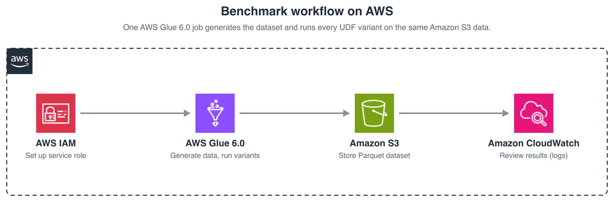
The following image shows the workflow of the benchmark.

Benchmark workflow on AWS

Figure 1: Benchmark workflow running each UDF variant as an AWS Glue 6.0 job

The high-level steps are:

  1. Set up the prerequisite AWS Identity and Access Management (IAM) role and Amazon Simple Storage Service (Amazon S3) bucket.
  2. Deploy and run the AWS Glue 6.0 job, which generates the dataset and runs the variants.
  3. Review the results, emitted to the job logs and optionally written back to Amazon S3.

The approaches we compared

All variants compute the same result. They differ in how data crosses the JVM–Python boundary and how the per-row logic runs.

Approach Transport (JVM–Python) Computation
standard Python UDF Pickle, one row at a time Python, per row
Arrow-optimized Python UDF (useArrow=True) Apache Arrow, columnar batch Python, per row
vectorized UDF (pandas UDF) Apache Arrow, columnar batch NumPy, per batch (through a pandas conversion)
native Arrow UDF (arrow_udf, Apache Spark 4.1) Apache Arrow, columnar batch PyArrow compute, per batch (no pandas conversion)
Spark SQL (built-in) None — runs on the JVM JVM, per batch

The vectorized UDF and the Arrow-optimized Python UDF both use Apache Arrow for transport, so both show ArrowEvalPython in the physical plan. The difference is the computation:

  • A vectorized UDF (pandas UDF) receives a pandas.Series (a batch of rows), so the computation can be expressed with NumPy and runs on the whole batch in native code. It involves a pandas conversion on top of Arrow.
  • An Arrow-optimized Python UDF is a scalar UDF: the function receives one value per call. Arrow makes the transport efficient, but the Python code still runs one row at a time.
  • A native Arrow UDF (the arrow_udf decorator, introduced in Apache Spark 4.1 and available in AWS Glue 6.0) receives and returns a pyarrow.Array and computes with PyArrow compute kernels. It operates directly on Arrow data, without the pandas conversion that a vectorized UDF performs.

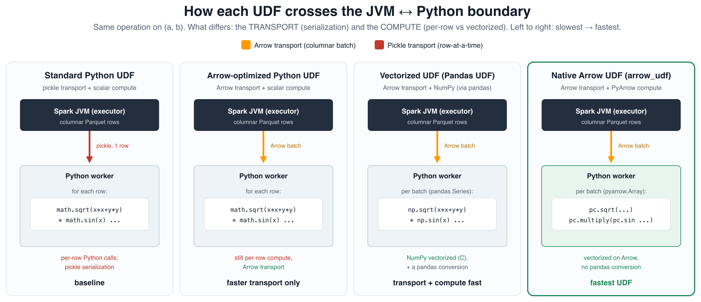
The following image summarizes how each variant crosses the boundary.

How each UDF crosses the JVM–Python boundary

Figure 2: How each UDF variant crosses the JVM to Python boundary

The code difference reflects that distinction. The registration shape is similar, but the computation differs:

# Arrow-optimized Python UDF: scalar function, Arrow transport
op = udf(lambda a, b: math.sqrt(a*a + b*b) * math.sin(a), DoubleType(), useArrow=True)

# vectorized UDF (pandas UDF): batch function, Arrow transport + NumPy computation
@pandas_udf(DoubleType())
def op(a, b):                       # a, b are pandas.Series (a batch of rows)
    return np.sqrt(a*a + b*b) * np.sin(a)

# native Arrow UDF: batch function, Arrow transport + PyArrow compute (no pandas)
@arrow_udf("double")
def op(a, b):                       # a, b are pyarrow.Array (a batch of rows)
    return pc.multiply(pc.sqrt(pc.add(pc.multiply(a, a), pc.multiply(b, b))), pc.sin(a))

Environment and setup

  • Runtime: AWS Glue 6.0 (Apache Spark 4.1.1, Python 3.13, Scala 2.13), 10 × G.1X executors plus the driver, in the US East (N. Virginia) AWS Region (us-east-1).
  • Data: A Parquet dataset with two bigint columns (a, b), written once to Amazon S3 and read back by every variant so all approaches read identical files.
  • Volumes: 10M, 50M, and 100M rows. Two dimensions are combined in every run: the workload (the per-row operation) and the query shape (how that operation is aggregated). Each of the three workloads was run under both query shapes, for every approach and volume.

Workloads (the per-row operation)

We chose three operations of increasing cost, to show how the results change as the per-row work shifts from “almost nothing” to “Python-only.”

Workload Per-row operation Why it’s included Applicable approaches
arith a + b The operation used in the AWS Prescriptive Guidance example. The computation is trivial, so serialization dominates the runtime. All five
mathheavy sqrt(x² + y²) · sin(x) + ln(y) Transcendental math with a meaningful per-row cost. It can be written in SQL, with PyArrow compute kernels, in NumPy, and in scalar Python, so all five approaches apply and compete. All five
pyheavy A bounded iterative loop (Collatz-style step count) Data-dependent control flow that can’t be expressed in SQL or with PyArrow compute kernels. This is the case where a Python UDF is the only option. Python UDF approaches only (no Spark SQL, no native Arrow UDF)

The progression matters. arith isolates the transport cost. mathheavy adds real computation, so vectorization can help. All five approaches apply, including the native Arrow UDF, because the math maps onto PyArrow compute kernels. pyheavy is the opposite extreme: an iterative loop that maps onto neither SQL nor PyArrow compute kernels, so Spark SQL and the native Arrow UDF don’t apply and only the Python-based UDFs remain.

Query shapes (how the operation is aggregated)

Each workload is measured under two query shapes, because they exercise different execution paths in the engine:

  • Streaming: sum(op(a, b)) — A full scan of every row, reduced to a single value. This isolates the per-row cost with minimal aggregation overhead.
  • Stateful: GROUP BY cast(op(a, b) AS bigint) % 1,000,000 — A full scan followed by a high-cardinality aggregation (about one million groups), which adds a shuffle and a large hash table.

Both shapes apply to all three workloads. To keep the tables readable, the following results report the streaming shape. We measured the stateful shape too and found the same ranking, with representative stateful figures given in the Results section.

Methodology

Two decisions had a material effect on the results.

Warm-up and best-of-N. The first run of each variant is dominated by cluster, JVM, and Python worker start-up. We ran one warm-up iteration that we discard, then N timed iterations, and report the best (and mean).

Reading fresh on every iteration. Our first attempt reused a cached DataFrame, and Spark cached the Parquet blocks and pruned the plan for a scalar count(). As a result the UDF timings didn’t scale with data size, and Spark SQL appeared slower than the UDFs. That was the opposite of the expected result. We corrected this by clearing the cache and re-reading the Parquet on every timed iteration, and by using sum(...) so the optimizer can’t prune the per-row work.

def bench(name, fn, repeat, warmup, pre=None):
    for _ in range(warmup):
        if pre: pre()
        fn()                     # discarded
    times = []
    for _ in range(repeat):
        if pre: pre()            # e.g. spark.catalog.clearCache()
        t = time.perf_counter(); fn(); times.append(time.perf_counter() - t)
    return {"best_sec": min(times), "mean_sec": sum(times) / len(times)}

After this correction, the ranking matched the AWS Prescriptive Guidance recommendation and remained consistent across volumes. In short: if a UDF benchmark doesn’t scale with row count, it’s likely measuring the cache rather than the computation.

Results

The following tables report the streaming query shape for each workload. We verified the stateful shape as well, and it produces the same ranking. For example, on mathheavy at 100M rows the stateful order matched streaming (Spark SQL 1.59 seconds, vectorized UDF 4.22 seconds, Arrow-optimized Python UDF 11.02 seconds, and standard Python UDF 14.33 seconds). The pyheavy table that follows shows the streaming and stateful columns side by side. The stateful figures run somewhat slower than streaming because of the added shuffle and hash aggregation, but the relative order of the approaches doesn’t change.

Workload 1: arith (a + b)

Best of seven iterations, warm-up excluded, streaming:

Approach 10M 50M 100M Relative to standard Python UDF (100M)
Spark SQL 0.53s 0.75s 0.99s 11.8× faster
native Arrow UDF (arrow_udf) 0.76s 1.79s 2.81s 4.2× faster
vectorized UDF (pandas UDF) 0.90s 1.98s 3.13s 3.7× faster
Arrow-optimized Python UDF 1.47s 4.82s 8.94s 1.3× faster
standard Python UDF 2.01s 6.20s 11.68s baseline

The recommended ranking holds, and the advantage of the vectorized UDF over the standard Python UDF widens with volume (from about 2.2× at 10M to 3.7× at 100M), because the standard Python UDF’s per-row serialization cost grows with the number of rows. For this trivial operation the native Arrow UDF and the vectorized UDF are close, because there is little computation to vectorize. Their advantage over the scalar approaches comes mainly from the columnar transport.

Workload 2: mathheavy

Best of 7 iterations, streaming:

Approach 10M 50M 100M
Spark SQL 0.52s 0.84s 1.22s
native Arrow UDF (arrow_udf) 0.72s 1.87s 3.13s
vectorized UDF (Pandas UDF) 0.79s 2.21s 3.83s
Arrow-optimized Python UDF 1.57s 5.79s 11.01s
standard Python UDF 1.80s 7.19s 13.82s

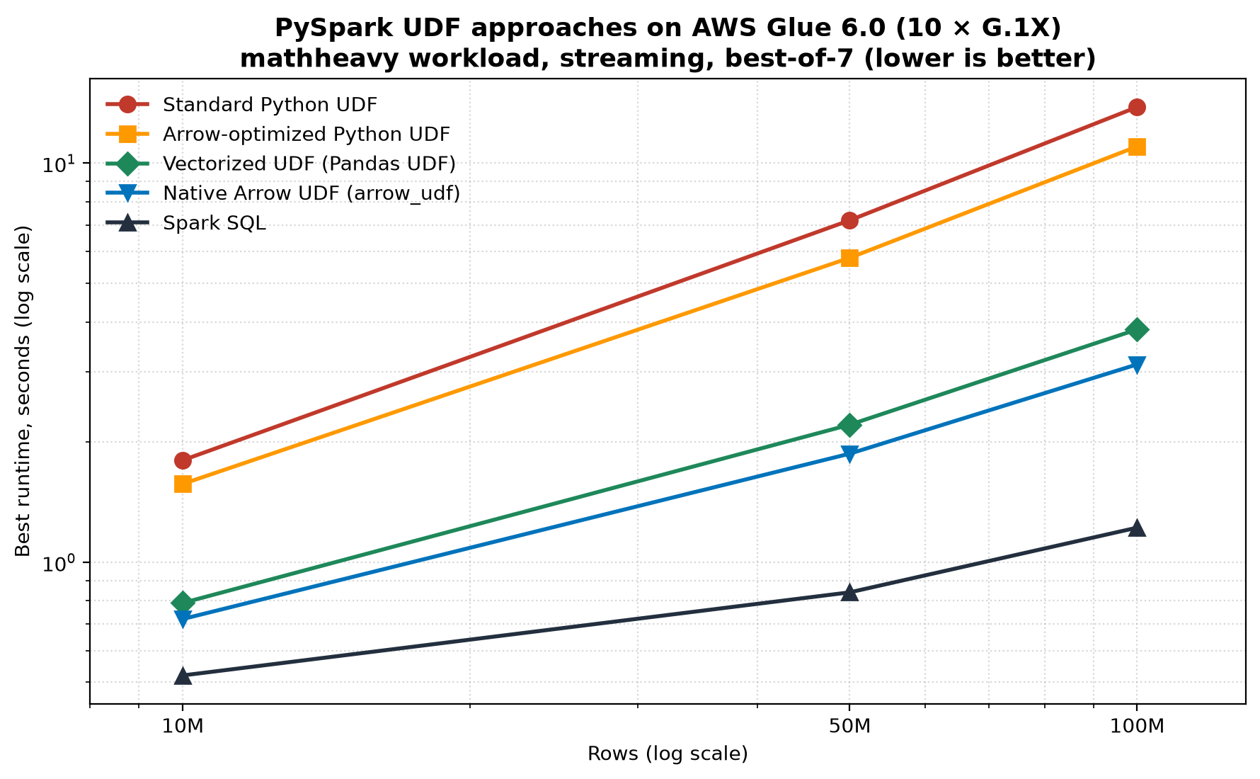
Among the UDF approaches, the native Arrow UDF was the fastest. It ran about 18 percent faster than the vectorized UDF at 100M (3.13 seconds versus 3.83 seconds) because it computes on Arrow data directly and avoids the pandas conversion. The timings scale approximately linearly across 10M, 50M, and 100M, and the ranking is stable at every volume. The following chart shows the approaches across volumes on a log-log scale.

PySpark UDF approaches across volumes

Figure 3: Runtime of each approach on the mathheavy workload across data volumes, on a log-log scale

Workload 3: pyheavy (no SQL equivalent)

This workload runs a per-row iterative loop with no closed-form equivalent. For each row it derives an integer from a and b and repeatedly applies the Collatz step (halve if even, otherwise 3n + 1) until the value reaches 1, counting the number of steps. To keep every row’s runtime predictable, the loop is bounded: it stops after at most 1,000 iterations even if it has not reached 1, so no single row can dominate the benchmark.

def collatz_steps(a, b):             # a, b are scalars (one row per call)
    n = int((a ^ b) % 100000) + 1
    steps = 0
    while n != 1 and steps < 1000:   # bounded: at most 1,000 iterations per row
        n = n // 2 if n % 2 == 0 else 3 * n + 1
        steps += 1
    return steps

This kind of data-dependent control flow can’t be expressed as a SQL scalar expression or with PyArrow compute kernels, so neither Spark SQL nor the native Arrow UDF applies, and only the Python-based UDF approaches are compared. The table shows both query shapes, at 10M, 50M, and 100M rows, to illustrate that the ranking is consistent across shapes and scales:

Approach 10M streaming 10M stateful 50M streaming 50M stateful 100M streaming 100M stateful
vectorized UDF (pandas UDF) 0.67s 0.72s 1.76s 1.85s 2.99s 3.01s
Arrow-optimized Python UDF 1.33s 1.36s 4.85s 4.86s 8.98s 8.71s
standard Python UDF 1.50s 1.55s 6.05s 6.28s 11.42s 11.73s

We report pyheavy up to 100M rows. Because Spark SQL and the native Arrow UDF don’t apply here, the only remaining options are the Python-based UDFs, whose timings scale near-linearly and whose relative order is already stable across both shapes by 100M.

This workload represents the case where a UDF is unavoidable. Examples include an iterative algorithm or a call into a Python library with no SQL counterpart that doesn’t map onto PyArrow compute kernels either. Here the vectorized UDF is the most effective available option: about 2.2× faster than the standard Python UDF at 10M, widening to about 3.8× at 100M.

A controlled experiment: Transport or computation?

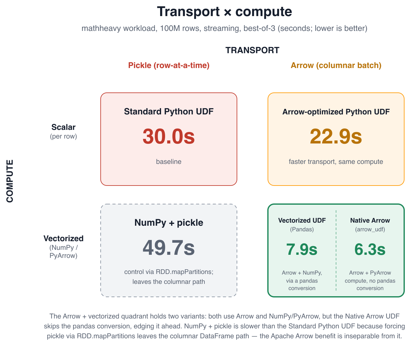
The vectorized UDF consistently outperforms the Arrow-optimized Python UDF. To test whether the difference comes from the transport (both use Arrow) or the computation (only the vectorized UDF uses NumPy on a batch), we constructed the missing combination (NumPy computation with pickle transport, no Arrow) using RDD.mapPartitions.

Transport and computation, as a 2×2

Figure 4: Transport and computation compared as a 2×2 experiment

The NumPy-with-pickle variant was the slowest of all (21.07 seconds at 100M, slower than the standard Python UDF at 13.82 seconds). The reason is that forcing pickle transport requires leaving the DataFrame API for RDD.mapPartitions, which changes two things at once. It materializes each row as a Python object before a NumPy array can be built, and it bypasses the optimized DataFrame execution engine that the vectorized UDF benefits from.

The practical conclusion is that the benefit of a vectorized UDF is not the Arrow transport in isolation. It’s Apache Arrow integrated into the vectorized DataFrame execution path. That path combines columnar transport and NumPy computation. Reproducing only the NumPy portion outside that path doesn’t yield the same benefit.

Code comparison: Arrow-optimized Python UDF and vectorized UDF

These two approaches are often confused: both use Apache Arrow for transport and both show ArrowEvalPython in the physical plan, so it’s worth seeing them side by side. The following two definitions compute the same mathheavy operation. The registration is almost identical. The difference is the function body and the type of its arguments.

The following code is an Arrow-optimized Python UDF (useArrow=True), where the function receives scalar values and runs once per row:

import math
from pyspark.sql.functions import udf
from pyspark.sql.types import DoubleType

def op(a, b):                        # a, b are scalars (one row per call)
    x = float(a % 100000) + 1.0
    y = float(b % 100000) + 1.0
    return math.sqrt(x * x + y * y) * math.sin(x) + math.log(y)

# Arrow transport, scalar Python computation
op_arrow = udf(op, DoubleType(), useArrow=True)
spark.udf.register("op_arrow", op_arrow)

df.selectExpr("sum(op_arrow(a, b)) AS r").collect()

The following code is a vectorized UDF (pandas UDF), where the function receives a pandas.Series (a batch) and computes with NumPy over the whole batch:

import numpy as np
from pyspark.sql.functions import pandas_udf
from pyspark.sql.types import DoubleType

@pandas_udf(DoubleType())
def op_pandas(a, b):                 # a, b are pandas.Series (a batch of rows)
    x = (a % 100000).astype("float64") + 1.0
    y = (b % 100000).astype("float64") + 1.0
    return np.sqrt(x * x + y * y) * np.sin(x) + np.log(y)   # NumPy, whole batch

spark.udf.register("op_pandas", op_pandas)

df.selectExpr("sum(op_pandas(a, b)) AS r").collect()

The following code is a native Arrow UDF (arrow_udf), where the function receives and returns a pyarrow.Array and computes with PyArrow compute kernels, operating directly on Arrow data with no pandas conversion:

import pyarrow as pa
import pyarrow.compute as pc
from pyspark.sql.functions import arrow_udf

@arrow_udf("double")
def op_native(a, b):                 # a, b are pyarrow.Array (a batch of rows)
    x = pc.add(pc.cast(pc.subtract(a, pc.multiply(pc.divide(a, 100000), 100000)), pa.float64()), 1.0)
    y = pc.add(pc.cast(pc.subtract(b, pc.multiply(pc.divide(b, 100000), 100000)), pa.float64()), 1.0)
    return pc.add(pc.multiply(pc.sqrt(pc.add(pc.multiply(x, x), pc.multiply(y, y))), pc.sin(x)), pc.ln(y))

spark.udf.register("op_native", op_native)

df.selectExpr("sum(op_native(a, b)) AS r").collect()

The Arrow-optimized Python UDF and the vectorized UDF differ in two lines that matter:

  • Argument type – In the Arrow-optimized UDF, a and b are scalars, so the body uses math.sqrt and math.sin and runs once per row. In the vectorized UDF, a and b are pandas.Series, so the body uses np.sqrt and np.sin and runs once per batch.
  • Where the computation runs – The Arrow-optimized UDF still executes Python per row. The vectorized UDF executes the batch in NumPy’s native code.

This difference in where the computation runs is what separates the three at scale. On the mathheavy workload at 100 million rows, the Arrow-optimized UDF ran in 11.01 seconds, the vectorized UDF in 3.83 seconds, and the native Arrow UDF fastest at 3.13 seconds. The native Arrow UDF edges ahead because it vectorizes the computation through PyArrow compute kernels without the pandas conversion the vectorized UDF performs. However, it requires the logic to be expressible with those kernels, where the vectorized UDF remains the more flexible choice.

Recommendations

These results align with the AWS Prescriptive Guidance recommendation and add a few practical points:

  1. Prefer built-in Spark SQL functions when the operation can be expressed in SQL – The computation runs on the JVM, and the advantage grows with data volume.
  2. When a UDF is required and the logic can be expressed with PyArrow compute kernels, consider a native Arrow UDF (arrow_udf) – In our tests it was the fastest UDF approach, because it vectorizes the computation on Arrow data without a pandas conversion. It’s available in AWS Glue 6.0 (Apache Spark 4.1).
  3. Otherwise, use a vectorized UDF (pandas UDF) – It outperformed the standard Python UDF by 2.2–3.8× in our tests. It’s the more flexible option when the logic is easier to express with pandas or NumPy than with PyArrow compute kernels.
  4. Arrow-optimized Python UDFs (useArrow=True) improve the transport but not the computation – They are faster than the standard Python UDF, but a vectorized or native Arrow UDF is faster whenever the per-row work is non-trivial. Consider the Arrow-optimized Python UDF when you want a minimal change to an existing scalar UDF.
  5. Stay in the DataFrame API to keep Arrow’s benefit – As the controlled experiment showed, the speedup doesn’t come from Arrow serialization alone. It comes from Arrow integrated into the vectorized DataFrame execution path. Applying the same NumPy logic through RDD.mapPartitions was the slowest approach of all, because it leaves that path. Implement vectorized logic as a vectorized or native Arrow UDF within the DataFrame API rather than dropping to the RDD API.
  6. For iterative or data-dependent logic (the pyheavy case), the vectorized UDF is the fallback – When the operation maps onto neither SQL nor PyArrow compute kernels, both Spark SQL and the native Arrow UDF are unavailable, and among the remaining Python UDF approaches the vectorized UDF was the most efficient.
  7. Decide whether the rewrite is worth the effort – Moving a scalar UDF to a vectorized or native Arrow UDF is a small code change, but it still has to be written and tested. As a rule of thumb, it pays off when the per-row work is non-trivial and the data is large or the job runs often. The speedup (and the per-second cost saving) scales with row count and with how frequently the job runs, while the rewrite is a one-time cost. For a trivial operation on a small, infrequent dataset, the standard Python UDF might be perfectly adequate. For a compute-heavy transform on hundreds of millions of rows that runs daily, the rewrite typically repays itself in the first few runs.
  8. The exact numbers depend on your cluster – All results here use a fixed configuration (10 × G.1X workers) on AWS Glue 6.0. The ranking of approaches is a property of how each UDF crosses the JVM–Python boundary and is not expected to change with cluster size. However, the absolute timings and any crossover with alternatives will shift with worker count, worker type, and data layout. Treat the figures as a guide to relative behavior and validate against your own configuration.
  9. Methodology affects the outcome – Warm-up handling and cache management changed our ranking. A UDF benchmark whose timings don’t scale with row count is likely measuring the cache.

Conclusion

The choice of UDF strategy has a measurable and recurring impact on both runtime and cost. On our compute-intensive workload at 100 million rows, the gap between the fastest UDF approach (the native Arrow UDF at 3.13 seconds) and the standard Python UDF (13.82 seconds) was about 4.4×, for identical output. Because AWS Glue bills by the second, that difference translates directly into spend on every job run.

These results extend the AWS Prescriptive Guidance recommendation with volume scaling from 10 million to 100 million rows, a compute-intensive workload, and the newer Arrow-based UDF options available in AWS Glue 6.0 (Apache Spark 4.1). As a methodology note, warm-up handling and cache management materially affected the ranking. A UDF benchmark whose timings don’t scale with row count is likely measuring the cache rather than the computation.

To learn more, see Optimize user-defined functions in AWS Prescriptive Guidance and the AWS Glue documentation.


About the author

Iván Fernández Perea

Iván Fernández Perea

Iván is a Senior Specialist Solutions Architect in Analytics at AWS, helping customers design data and analytics platforms. He combines a software engineering background in cloud and big data with years of experience as a lecturer in big data and cloud computing at universities and business schools in Spain.

How Thermo Fisher Scientific built AI-powered patient matching on AWS

Post Syndicated from Kaushal Patel original https://aws.amazon.com/blogs/architecture/how-thermo-fisher-scientific-built-ai-powered-patient-matching-on-aws/

Clinical trial recruitment is often described as a patient-matching challenge. In practice, it is much broader. Patient Recruitment teams need to understand where potential participants are in the recruitment journey, how sites are performing, which geographies may offer the strongest opportunities, and whether enough patients may meet increasingly complex study criteria. The answers often sit across different systems, datasets, surveys, questionnaires, consent records, marketing interactions, and operational workflows.

For Thermo Fisher Scientific, improving that experience required more than introducing a new application. It required rethinking the data foundation supporting patient recruitment and creating a more scalable way to turn recruitment data into actionable insights.

Using AWS, Thermo Fisher Scientific established a modern patient recruitment data foundation which brings together and curates data for analytics and AI-enabled use cases. Built on this foundation are complementary capabilities including Patient Recruitment’s Central Insights Hub (CIH), which provides recruitment analytics and operational visibility, and Patient Match AI, Thermo Fisher Scientific’s proprietary tool, that supports self-service patient search, feasibility assessment, and cohort discovery through natural-language interaction.

The impact is particularly visible in cohort discovery. Questions that could previously involve days or even weeks of analysis and back-and-forth with technical teams can now be explored and refined in minutes, giving recruitment teams a faster path from a question to an actionable patient population.

As these capabilities moved toward production, Thermo Fisher Scientific also worked with AWS Countdown Premium to strengthen operational readiness, support launch activities, and reduce risk during a critical stage of the transformation.

The challenge

Over time, patient recruitment data had grown across multiple systems and use cases. Patient information, surveys and questionnaires, recruitment funnel activity, marketing interactions, consent information, site data, and other operational datasets did not always exist in a single, consistent form.

That fragmentation created several challenges.

Recruitment teams needed faster ways to identify and refine relevant patient populations across large volumes of records. They also needed a clearer view of recruitment performance across studies, sites, and geographies. At the same time, the organization wanted to introduce AI-enabled capabilities without compromising data quality, privacy, governance, or compliance.

Existing processes often depended on specialized technical teams to translate business or clinical questions into database queries, retrieve the appropriate data, validate the results, and then repeat the process as criteria changed.

For a simple question, that approach could be manageable. For complex cohort discovery involving multiple clinical, demographic, geographic, or consent-related criteria, it could become a lengthy iterative process.

Thermo Fisher Scientific therefore faced two connected challenges: modernizing the patient recruitment data environment and making that data easier for business users to explore and act on.

Building the data foundation first

Rather than treating AI as a layer that could simply be added to existing systems, the team started with the data. Thermo Fisher Scientific established a modern patient recruitment data foundation on AWS to bring together information from previously disconnected sources and prepare it for downstream analytics and intelligent applications.

The new foundation standardizes and curates data from sources such as patient profiles, surveys, questionnaires, recruitment funnel activity, marketing information, consent data, and other recruitment datasets. Data transformations help create more consistent structures and reusable datasets for applications that depend on them.

This approach provides an important separation of concerns: source systems continue to serve their operational purposes, while curated datasets are prepared specifically for analytics, reporting, and AI-driven workloads.

For the business, the result is a more trusted and reusable source of recruitment information. For technology teams, it creates a scalable foundation that can support multiple products instead of building separate data pipelines for every new use case.

Turning recruitment data into operational insight with Central Insights Hub

One of the capabilities supported by this broader modernization is Central Insights Hub (CIH), Thermo Fisher’s in-house custom UI layer built using open-source technologies.

CIH is a centralized clinical trial recruitment analytics platform that helps teams understand how recruitment efforts are performing across studies.

Through interactive dashboards and visualizations, users can follow the recruitment journey from initial patient engagement through milestones such as pre-screening, referral to a study site, consent, enrollment, and randomization.

The platform brings together views of patient progression, site activity, recruitment timelines, geographic performance, and other operational measures. As CIH has evolved, additional capabilities have expanded visibility into areas such as recruitment costs, participant demographics, disqualification trends, site-patient engagement, and marketing-channel performance.

This gives recruitment teams a common place to identify bottlenecks, compare activity across sites and countries, understand where additional attention may be required, and make more timely decisions.

CIH shows how recruitment is performing and where teams should focus.

Making cohort discovery self-service with Patient Match AI

Patient Match AI, an internal tool within Thermo Fisher, addresses a different, but complementary, challenge: helping users quickly determine which patient populations may be relevant to a recruitment need.

Instead of asking a technical team to manually construct database queries, users can describe what they are looking for in natural language.

For example, a user may begin by asking for the number of patients who meet a broad clinical condition. They can then progressively refine that population by age, geography, diagnosis, treatment history, demographic characteristics, consent or contactability criteria, and other available attributes.

The intended experience follows a straightforward progression:

COUNT → REFINE → TARGETED LIST → EXPORT

Users can start by understanding the size of a potential population, refine the criteria as they learn more, and then move toward a targeted patient cohort when appropriate.

This changes the working model from a series of handoffs to a more interactive, self-service experience.

Tasks that previously could require several rounds of analysis over days or weeks can, for many common feasibility workflows, now be explored in minutes. Recruitment teams can test assumptions, adjust criteria, and understand how those changes affect the potential population without restarting the process each time.

Patient Match AI also supports aggregate insights and visualizations, helping users better understand the composition of a cohort before progressing to governed workflows when patient identity information is required.

Privacy, governance, consent, contactability, and personally identifiable information (PII) controls, consistent with applicable regulatory requirements, remain an important part of the design. The objective is not unrestricted access to patient data, but a faster and more intuitive way to work within established recruitment and governance processes.

Architecture overview

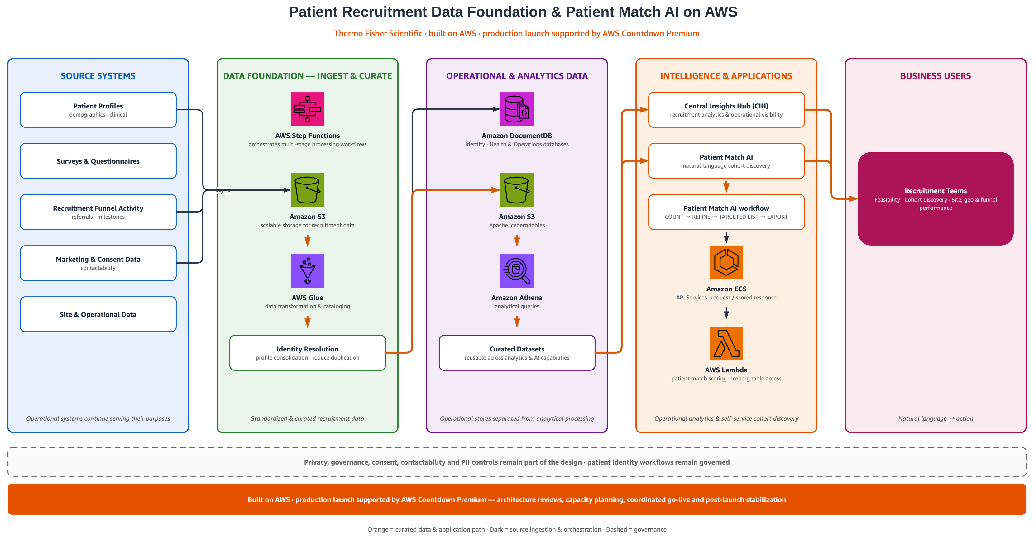
The following diagram shows how data moves from source systems through the curated data foundation into Patient Match AI and Central Insights Hub, and the key AWS services involved at each stage.

Data flowing from source systems through the curated AWS data foundation into Patient Match AI and Central Insights Hub

Figure 1: How data moves from source systems through the curated data foundation into Patient Match AI and Central Insights Hub

The solution uses a cloud-native architecture on AWS that combines managed services for data storage, transformation, orchestration, analytics, AI workloads, and application delivery.

Amazon Simple Storage Service (Amazon S3) provides scalable storage for recruitment data, while AWS Glue supports data transformation and cataloging. AWS Step Functions orchestrates multi-stage data processing workflows, and Amazon Athena runs analytical queries across curated datasets.

The analytics layer uses Apache Iceberg tables on Amazon S3, providing a flexible foundation for large-scale analytical workloads and supporting continued growth in both data volume and use cases.

A key architectural principle is the separation of operational application workloads from analytical processing. Complex cohort and eligibility queries can therefore run across large volumes of patient profiles without placing the same workload on transactional application databases.

Thermo Fisher’s identity resolution and profile consolidation processes also help bring together records originating from multiple systems, reducing duplication and establishing a more consistent view for downstream recruitment use cases.

The outcome is not simply a collection of cloud services. It is an architecture designed so that data can be ingested, curated, queried, and reused across analytics and AI capabilities without rebuilding the underlying foundation for every product.

Source systems include patient profiles, surveys and questionnaires, recruitment funnel activity, marketing and consent data, and site and operational data. These sources are ingested into the data foundation. There, AWS Step Functions orchestrates multi-stage processing, Amazon S3 provides storage, and AWS Glue handles transformation and cataloging. An identity resolution step consolidates profiles and reduces duplication.

Curated data then flows into two separated stores. Amazon DocumentDB (with MongoDB compatibility) holds identity, health, and operations data. The team selected it as the closest managed equivalent to the MongoDB database they had previously relied on. Amazon S3 with Apache Iceberg tables, queried through Amazon Athena, holds the analytics data.

These curated datasets feed the intelligence layer. Central Insights Hub provides recruitment analytics, and Patient Match AI supports natural-language cohort discovery through a COUNT, REFINE, TARGETED LIST, and EXPORT workflow. Amazon Elastic Container Service (Amazon ECS) hosts the API layer, and AWS Lambda performs patient match scoring. Results reach recruitment teams for feasibility, cohort discovery, and site, geographic, and funnel performance analysis. Throughout, privacy, governance, consent, contactability, and PII controls remain part of the design.

Preparing for production with AWS Countdown Premium

Building technology was only part of the journey. Moving a large-scale recruitment capability into production required confidence that the architecture, capacity, operating procedures, and support model were ready for launch.

Thermo Fisher Scientific engaged AWS Countdown Premium from the testing phase onward.

AWS Countdown Premium is an engineer-led support service that provides designated expertise and guidance across critical phases of cloud projects. For this engagement, that support helped the team prepare for launch in four key areas.

Designated engineering expertise

A specialist engineer selected from a team of AWS experts served as a consistent technical point of contact and developed a deeper understanding of the Patient Match AI architecture.

That continuity was valuable when working through complex technical issues. Rather than rebuilding context for each support interaction, the team could work with an engineer who was already familiar with the system and could coordinate access to additional AWS subject matter experts when needed.

One example from the engagement:
Pipeline design review: An AWS specialist engineer reviewed key design decisions ahead of launch. The patient scoring logic moved away from retrieving every record before ranking, and the pipeline was parallelized before sorting and querying. For long-running external calls in AWS Step Functions, the team adopted the wait-for-callback pattern, so they pay only for state transitions and not for idle wait time.

Operational readiness and proactive planning

The engagement focused on identifying potential issues before production rather than waiting for them to appear during launch.

Pre-event reviews, capacity planning, operational runbooks, and decision frameworks helped the team validate that the environment was prepared to support large-scale patient recruitment workloads.

Another example from the engagement:
AWS Glue readiness review: An AWS Glue specialist reviewed the team’s extract, transform, and load (ETL) jobs in non-production and shared written recommendations before launch. The team also received guidance on reading Apache Iceberg tables through the AWS Glue Iceberg REST endpoint and on putting AWS Glue Studio visual jobs under source control.

Support during go-live

During launch, coordinated AWS support provided another layer of technical coverage for troubleshooting and issue resolution.

For a production system supporting clinical recruitment workflows, this helped the team move through go-live with greater confidence and a clear escalation path for issues requiring AWS expertise.

Post-launch stabilization

Support continued beyond the initial deployment.

This provided continuity as the team monitored production behavior, addressed early issues, and transitioned from launch activities into normal operations.

Results

By combining a modern cloud architecture with support from AWS Countdown Premium, Thermo Fisher Scientific achieved several key outcomes:

  • Unified patient data – More than 20 million patient profile records, about 1.6 TB, were brought together from previously separate sources, including patient profiles, surveys, questionnaires, recruitment funnel data, marketing information and consent data.
  • Self-service cohort discovery – With Patient Match AI, recruitment teams can find and refine patient populations by asking questions in plain language, and the shared test queries run in under six seconds against the full dataset.
  • Faster feasibility analysis – Cohort analysis now takes minutes as opposed to days for many common feasibility and patient discovery workflows.
  • More timely insights – Recruitment data is kept up to date continuously, so it is available right away for AI-driven patient search and shortly afterward for analytics dashboards.
  • Modernized data foundation – The move to a data foundation built on AWS reduces reliance on the earlier Snowflake-backed dashboard environment.
  • Successful production launch – Patient Match AI went live in production in Q2 FY26. AWS Countdown Premium supported the launch through an architecture review, readiness reviews for Amazon DocumentDB and AWS Glue, and expert guidance on workflow design and query optimization over a four-month engagement.
  • Designated engineering support – A dedicated Countdown Premium engineer worked with the Amazon DocumentDB service team and specialists to tune the database, cutting estimated processing time by more than 3x.
  • Lower launch risk – Testing at full scale against the complete 20 million record dataset exposed query performance problems early, so they could be fixed before go-live.

Looking ahead

The broader value of this transformation goes beyond any single application. Thermo Fisher Scientific has established a modern, curated patient recruitment data foundation that can support different types of experiences, from operational analytics in Central Insights Hub to AI-powered cohort discovery through Patient Match AI, and that shared foundation creates an opportunity to continue evolving recruitment capabilities without repeatedly rebuilding the underlying data infrastructure.

More importantly, it changes how recruitment teams can work with data.

Instead of waiting for information to move through multiple technical handoffs, teams can increasingly interact with trusted recruitment data directly, using dashboards to understand what is happening and natural-language tools to explore what may be possible.

Conclusion

Thermo Fisher Scientific’s modernization of its patient recruitment environment, including a modern, curated patient recruitment data foundation, Central Insights Hub (CIH), and Patient Match AI, demonstrates how organizations can combine modern data architecture, analytics, and AI capabilities to solve complex, high-stakes business problems.

By using AWS services for data management, orchestration, analytics, and AI, the team created an environment that makes recruitment information easier to access, understand, and act on. Processes that once required substantial manual analysis can now be more timely, interactive, and self-service.

AWS Countdown Premium played an important role in de-risking the transition to production. Designated engineering support, proactive planning, launch assistance, and post-launch stabilization helped the team move these capabilities into production with greater confidence and operational readiness.

For Thermo Fisher Scientific, the result is more than a technology modernization. It is a foundation for helping recruitment teams move from data to insight, and from insight to action, faster.

Other organizations have used AWS Countdown Premium for similar initiatives, from improving manufacturing operations to seamless website migration and accelerating critical cloud migrations.

To learn more about how AWS Countdown Premium can support your next critical cloud initiative, reach out to your AWS account team.

Acknowledgements

Special thanks to everyone who contributed to this launch:

  • Patient Recruitment Engineering Team: Prameela Yasa, Madhurendra Singh, Prakash Singh, Karthik Tirumalasetti, Thanmay Jasti Naga Chowdry, Pawan Shah, Arnab Ghosh, Denys Martsynko, Maria Ozirskaya, Daniel Petko.
  • AWS Leadership: Kwesi Edwards, Mary Marzak.


About the authors

Kaushal Patel

Kaushal Patel

Kaushal is Director of Engineering within CRG Digital at Thermo Fisher Scientific, where he leads the CRG Digital Engineering Team and drives the architecture and delivery of next-generation digital recruitment solutions.

Venu Rapolu

Venu Rapolu

Venu is a Technical Account Manager (TAM) at Amazon Web Services, based in Seattle, WA. He specializes in Cloud Operations, with a primary focus on Cloud Financial Management (CFM) and FinOps. Venu partners with enterprise customers to accelerate cloud adoption, optimize cost, and drive operational excellence at scale. Away from the keyboard, Venu is passionate about community volunteering and spending quality time with his family.

Ram Pathangi

Ram Pathangi

Ram is a Senior Solutions Architect at AWS supporting healthcare and life sciences customers in the San Francisco Bay Area. He has helped customers in Finance, Healthcare, Life Sciences, and Hi-Tech verticals run their business successfully on the AWS Cloud. He specializes in Databases, Analytics, and Machine Learning. Outside of work, he enjoys traveling and meditating.

Amazon Threat Intelligence observes threat actors running cybercrime campaigns with Artex AI agents

Post Syndicated from CJ Moses original https://aws.amazon.com/blogs/security/amazon-threat-intelligence-observes-threat-actors-running-cybercrime-campaigns-with-artex-ai-agents/

From Oct. 3 to Nov. 5, 2026, Amazon’s MadPot, a globally distributed network of decoy threat sensors, captured requests from AI agents that included operating memory from offensive campaigns that threat actors ran on ARTEX, an open-source agentic AI penetration testing framework. The ARTEX agents sent these requests to MadPot sensors configured to present as popular large language model (LLM) inference APIs, and the requests carried the agents’ own records of their campaigns.

Amazon Threat Intelligence assessed threat activity referencing potentially affected AWS customers and notified them as appropriate. Because activity against other organizations could not be confirmed, this post shares the findings and indicators of compromise (IOCs) so that organizations that run the affected technologies can review their own environments.

The most prominent ARTEX campaign was a large-scale theft of credentials to access AI models, organized as a self-sustaining operation in which stolen keys paid for the LLM inference powering further credential hunting. Another campaign targeted cryptocurrency exchanges for know-your-customer (KYC) verification bypass using real-time deepfake injection. In aggregate, the agent records show that agentic frameworks have progressed from experimental use to sustained, multi-objective offensive operations that run with minimal human intervention. This post describes how these campaigns operated based on the agents’ own descriptions of the campaigns.

Attribution and instructions

Amazon Threat Intelligence assesses with moderate confidence that ARTEX was used for these campaigns due to prompt references to ARTEX tooling and other technical artifacts referencing ARTEX. Threat actors instructed ARTEX agents through standing instruction prompts that set the mission objectives, targeting rules, and operational constraints. Within those instructions, the agents handled the work themselves. In one credential theft campaign, operators told the agents to work through a fixed sequence of countries, prioritize enterprise production sites over personal projects, and grade every stolen credential by whether it worked and what it could reach. Agents were directed to treat credentials exposed publicly for more than 30 days as low-value inventory.

Amazon Threat Intelligence also assess with moderate confidence these are disparate Chinese-nexus threat groups due to use of simplified Chinese language in prompts, China time-zone configurations, targeting consistent with Chinese interests, and tooling predominantly used by Chinese-nexus threats. Sample instructions included setting red lines, such as excluding mainland China targets and government domains, and required all outbound traffic to go through proxies.

How MadPot saw inside these campaigns

MadPot presents controlled services to potential attackers and records how they discover, test, and attempt to compromise or abuse them. MadPot telemetry allows Amazon Threat Intelligence to observe attacker behavior without exposing customer workloads. In this case, the MadPot sensors presented popular LLM-compatible chat-completions interfaces on various ports. Agentic frameworks sent prompts to these interfaces as part of their offensive workflows, treating them as LLM inference backends.

The resulting telemetry contained the persistent task context, system prompts, tool histories, knowledge-graph state, and reported findings that these frameworks ordinarily send to an LLM to make operational decisions. Because agentic frameworks retain the history of past conversations, individual requests often contain the full operational history of a campaign. That history described activity that occurred before and between the captured requests, on systems MadPot does not monitor. Amazon Threat Intelligence did not observe that activity as it happened and cannot verify the outcomes the agents reported, but the records show what the actors were pursuing.

Most of the activity used ARTEX to divide work among planner, worker, verification, and compression agents sharing a persistent knowledge graph. The knowledge graph acts as the operation’s shared memory: every agent reads from it, and writes its results back, so each agent picks up where the others left off. The agents’ records described reconnaissance, vulnerability testing, credential theft, cloud-privilege expansion, and cryptocurrency fraud attempts across hundreds of targets spanning AI application platforms and other workloads. These records show how threat actors are organizing persistent, financially motivated offensive operations using agentic AI frameworks.

Campaign 1: Stealing AI credentials at industrial scale

In this campaign, threat actors used AI agents to steal API keys and other credentials that grant access to AI models, most likely so they could use those models while someone else paid for them. The agents’ records show stolen keys being fed into the framework’s own model gateway, where they powered the agents searching for more keys. Beyond AI model access keys, cloud credentials were treated as a doorway to more access. Agents validated identities through each provider’s token and identity services, enumerated storage, assessed permission scope, and went after managed AI model services, secrets and parameter stores, and application identities. They prioritized access to premium frontier models over general cloud permissions.

Agents recorded use of different AI gateways, keys, and models, but they all used a shared method: find internet-exposed AI applications, extract the upstream provider keys they hold, validate those keys, and store them in a managed pool. The agents focused on applications that aggregate provider keys, because one weak management interface can expose many downstream accounts. Targets included LLM gateways and proxy platforms such as One API, New API, Veloera, Sub2API, and LiteLLM, and AI application builders such as Dify, FastGPT, Langflow, RAGFlow, Open WebUI, LobeChat, and Ollama. A codified vulnerability playbook mapped each fingerprinted product to its known attack chain, including uninitialized installs that could be claimed, anonymous management and provider-configuration endpoints, default administrator credentials, such as the LiteLLM default master key, CVE-2025-3248 (Langflow), CVE-2026-28797 (RAGFlow), an authentication bypass via the isCliRequest header in One API family systems, SSRF through URL-fetch features to cloud metadata services, and secrets left in client-side JavaScript, source maps, debug routes, and environment files.

To find those keys, discovery drew on internet scanning services, certificate transparency, and public code and artifact sources: GitHub repositories and event archives (targeting secrets that fell outside automated revocation), npm and PyPI tarballs, container image layers, notebooks, model-hosting spaces, paste sites, and Telegram channels. One parallel operation worked through a fixed country sequence, prioritizing enterprise production sites, and graded every credential: L1 for a lead, L2 for a confirmed working API call, and L3 for quantified impact, such as readable data or spendable balance. Keys exposed publicly for more than 30 days were treated as low-value inventory.

Campaign 2: Defeating identity verification with deepfakes

In this campaign, threat actors used AI agents to defeat the identity verification (KYC) checks at two cryptocurrency exchanges with deepfakes. The agents’ records show generating real-time deepfake video to pass live selfie checks and forged ID document photos to pass document checks.

The records describe a methodical approach to the liveness check, which is a security method that confirms a person interacting with a digital system is a real, living human being physically present at the time of capture. The agents reverse-engineered one vendor’s liveness protocol in detail, documenting the face-detection event stream it sends, how it tracks face position during the check, and the coordinate system it uses to tell the user where to move. Their best recorded attempt completed the full movement sequence with the face positioned within 7 pixels of the target. Even so, the vendor’s server-side verdict rejected the deepfake in every attempt the agents recorded. In parallel, a separate session built a real-time deepfake video pipeline on a single consumer-grade GPU using an open-source face animation model. By splitting the model and avoiding unnecessary memory copies on the GPU, it reached 11.5 frames per second, close to what a live video check expects.

The agents worked on the ID document as well. Verification vendors look for signs that a document photo was edited or is a picture of a screen rather than a camera capture. To get past those checks, the agents recorded building synthetic camera metadata whose image dimensions matched the real values inside the JPEG file, and preserving the original camera compression tables that re-saving an edited image would normally replace. The result is an altered image that looks, at the file level, like an untouched camera photo.

This campaign also shows how ARTEX runs several workstreams toward one goal. At least four agent sessions ran at once: one searched for ways to cash out, one worked on clearing account balances, one set up the deepfake video pipeline, and one carried out the verification bypass. They shared findings and handed off tasks through cross-session tools.

What this means for defenders

None of the techniques in these campaigns were new. What AI agents change is the speed and persistence of the attacker. The agents succeeded where basic security hygiene was missing, including default or hardcoded credentials, keys left in code and public artifacts, unauthenticated interfaces and inference endpoints, and unpatched software. Getting those fundamentals right remains the most effective defense.

Given the speed and persistence of the attackers, organizations should assume exposed secrets and misconfigurations will be found quickly and remediate accordingly. They should bring AI applications, model gateways, and inference endpoints under the same controls as other production systems, and they should watch for misuse of AI services through unexpected spend or unusual usage.

Indicators of Compromise (IOCs)

IOC Value IOC Type First Seen Last Seen Annotation
104.28.225[.]223 IPv4 2026-10-17 2026-10-19 Campaign 1
31.22.91[.]156 IPv4 2026-10-14 2026-10-19 Campaign 1
150.136.38[.]110 IPv4 2026-10-31 2026-10-31 Campaign 1
128.242.115[.]131 IPv4 2026-10-31 2026-10-31 Campaign 1
216.176.239[.]231 IPv4 2026-11-02 2026-11-02 Campaign 1
212.107.28[.]51 IPv4 2026-10-14 2026-10-14 Campaign 2
103.142.140[.]158 IPv4 2026-10-17 2026-10-17 Campaign 2
104.28.251[.]98 IPv4 2026-10-18 2026-10-18 Campaign 2
104.28.251[.]99 IPv4 2026-10-18 2026-10-18 Campaign 2
104.28.219[.]97 IPv4 2026-10-18 2026-10-18 Campaign 2
125.103.213[.]41 IPv4 2026-10-18 2026-10-19 Campaign 2

If you have questions, start a new thread on AWS re:Post or reach out to AWS Support.


CJ Moses

CJ Moses

CJ Moses is the CISO of Amazon Integrated Security. In his role, CJ leads security engineering and operations across Amazon. His mission is to enable Amazon businesses by making the benefits of security the path of least resistance. CJ joined Amazon in December 2007, holding various roles including Consumer CISO, and most recently AWS CISO, before becoming CISO of Amazon Integrated Security September of 2023.

Prior to joining Amazon, CJ led the technical analysis of computer and network intrusion efforts at the Federal Bureau of Investigation’s Cyber Division. CJ also served as a Special Agent with the Air Force Office of Special Investigations (AFOSI). CJ led several computer intrusion investigations seen as foundational to the security industry today.

CJ holds degrees in Computer Science and Criminal Justice, and is an active SRO GT America GT2 race car driver.

Kitesurf is now open source

Post Syndicated from Celso Martinho original https://blog.cloudflare.com/kitesurf-open-source/

We introduced Kitesurf, our stateless browser for AI agents that runs entirely on top of Workers, in August and followed up in September with WebMCP support, new APIs, and improved compatibility. On every occasion, we mentioned our commitment to open sourcing it so that developers could run their own browser engine on their own Cloudflare accounts if they want to.

That promise is now real. Kitesurf is open source on GitHub under the Apache 2.0 license. You can read the code, run it locally, change it, and deploy your own instance to Cloudflare Workers.

A browser built for agents

Kitesurf runs entirely on Cloudflare Workers. It parses HTML, applies CSS, executes page JavaScript, and renders screenshots without a browser container. It supports the Chrome DevTools Protocol (CDP), so you can connect clients such as Puppeteer.

Our main goal is to give AI agents a lightweight, efficient browser — one that can load websites, execute JavaScript, and interact with pages while using less CPU and memory than a full browser like Chromium, and scaling on demand across Cloudflare’s global Workers network.

Read more about why and how we built Kitesurf in our initial announcement and how to use it in Browser Run’s developer documentation.

What is inside the repository?

Kitesurf builds on Cloudflare’s Developer Platform and APIs, alongside an ecosystem of open-source Rust packages compiled to WebAssembly:

  • Blitz provides HTML parsing, the DOM, layout, and painting.
  • Stylo provides CSS parsing, cascading, and computed styles.
  • Boa runs JavaScript inside WebAssembly (as the last resort only when we can’t run JavaScript in Dynamic Workers).
  • Linebender libraries provide text layout and 2D graphics, and Krilla generates PDF output.

These projects made Kitesurf possible. They retain their respective licenses; the repository's NOTICE documents third-party notices.

Kitesurf has three main parts: the Engine manages browser sessions and client connections, PageScript runs the page and its JavaScript, and PageRenderer draws the result.

All packages, the engine, its Rust core, DOM shims, renderer, and Kitesurf CLI live separately in folders under the repository’s packages directory where you can explore how all the pieces fit together.

Run your own Kitesurf

To run Kitesurf locally, follow the repository's build requirements, then clone the repository, install dependencies, and start the engine:

git clone https://github.com/cloudflare/kitesurf.git
cd kitesurf
pnpm install --frozen-lockfile
pnpm run dev

The first build compiles the Rust core and its dependencies, so give it some time. Subsequent builds reuse the build cache. Finally wrangler starts a local development server at http://127.0.0.1:8787. Open that address to try a page in Chrome DevTools, or use it programmatically.

You can use puppeteer with a NodeJS script:

import puppeteer from "puppeteer-core";

const browser = await puppeteer.connect({
  browserWSEndpoint: "ws://127.0.0.1:8787/devtools/browser",
});

try {
  const page = await browser.newPage();
  await page.goto("https://example.com/");
  await page.screenshot({ path: "page.png" });
} finally {
  await browser.disconnect();
}

Or you can point your AI harness at the local CDP port (agents love CDP) and watch it take full control of Kitesurf.

Deploy to your Cloudflare account

When you’re done changing and testing locally, you can deploy the engine to your own account and use Kitesurf from there instead of the Browser Run managed APIs we provide. Note that a Workers Paid plan is required because Kitesurf uses Dynamic Workers to create isolated Workers for pages.

From the repository root:

pnpm run deploy

Help us make it better

As with all of our open-sourced projects, Kitesurf lives in Github and we welcome forks and contributions. However, note that Kitesurf is under heavy development and we are focusing on making the engine more compatible (check out Web Platform Test evolution), more reliable, and efficient.

Start with the contribution guidelines if you want to contribute. Open an issue with a minimal reproduction or a proposed approach, and get vouched by a maintainer before opening a pull request. Focused fixes with tests, clear evidence, and a well-defined scope are much easier to review than large rewrites or unrelated cleanup, but all contribution does not have to be code: a small page that reproduces a rendering bug, a failing automation workflow, or a clear documentation correction can help us move forward.

Stay tuned

Kitesurf is evolving quickly. Stay tuned for updates in the blog and our changelog, and keep an eye on the official landing page for the latest on standards compatibility in Web Platform Tests page and benchmarks.

And come chat with the team on Discord. We’re building a browser for agents, and we’d love your help making it better.

Multi-statement transactions for Apache Iceberg tables in Amazon Redshift

Post Syndicated from Shiyu Xu original https://aws.amazon.com/blogs/big-data/multi-statement-transactions-for-apache-iceberg-tables-in-amazon-redshift/

Data pipelines often change a table in several steps, such as first upserting the day’s sales and then removing canceled orders. Amazon Redshift now supports multi-statement transactions for Apache Iceberg tables so you can run several data manipulation language (DML) statements against one Iceberg table inside a single BEGIN … COMMIT. Amazon Redshift publishes them as one Iceberg snapshot. Readers in other sessions and engines see the table before the batch commit or after it. A failed or rolled-back transaction leaves nothing to undo. Multi-statement transactions are available in Amazon Redshift with Patch 206 and later.

Multi-statement transactions extend existing Iceberg support in Amazon Redshift, which you can use to create Iceberg tables and write to them with INSERT, modify rows with DELETE, UPDATE, and MERGE, store materialized views as Iceberg tables, and commit concurrent writes that don’t overlap. Until now, though, each write committed on its own, one statement at a time.

In this post, we explain why one commit per statement makes multi-step pipelines fragile and how Amazon Redshift commits multiple statements as one snapshot. We also cover what you can run in a transaction, what concurrent readers and writers see, and how multi-statement transactions perform.

The challenge of one commit per statement

Consider a retailer whose finance team tracks daily revenue. During the day, some point-of-sale (POS) values are corrected, such as a price fix, and others are voided, such as a canceled order. Dashboards and downstream jobs read revenue from one Iceberg table, sales (sale_id, store_id, sale_date, amount), in the external schema iceberg_schema. Each night, the POS system delivers the day’s batch as two staging Iceberg tables. pos_sales holds new and corrected sales, one row per sale_id, and pos_voids lists voided sales. A job applies the batch in two statements:

-- 1. Upsert new and corrected sales
MERGE INTO iceberg_schema.sales USING iceberg_schema.pos_sales p
  ON sales.sale_id = p.sale_id
  WHEN MATCHED THEN UPDATE SET amount = p.amount
  WHEN NOT MATCHED THEN INSERT VALUES (p.sale_id, p.store_id, p.sale_date, p.amount);
-- auto-commits: revenue includes voided sales

-- 2. Remove voided sales
DELETE FROM iceberg_schema.sales
  WHERE sale_id IN (SELECT sale_id FROM iceberg_schema.pos_voids);
-- auto-commits: revenue is correct

Because each statement commits on its own, the state between them is public. Until the DELETE commits, every reader sees revenue that includes the voided sales. If the DELETE fails, for example because the query is canceled, the table stays that way. If a check after the job finds the batch wrong, both changes are already public, so you must work out which statements landed and write SQL to undo them. Each commit also costs time as it writes new table metadata to Amazon Simple Storage Service (Amazon S3) and updates the catalog. A job of N statements pays the catalog update N times.

How Amazon Redshift commits multiple statements as one snapshot

To make the batch atomic, wrap the same statements in BEGIN and COMMIT. No new syntax is needed, and the job can audit the result before it commits:

BEGIN;

-- 1. Upsert new and corrected sales (full statement above)
MERGE INTO iceberg_schema.sales USING iceberg_schema.pos_sales p ON ...;

-- 2. Remove voided sales
DELETE FROM iceberg_schema.sales
  WHERE sale_id IN (SELECT sale_id FROM iceberg_schema.pos_voids);

-- 3. Audit: data quality checks see the uncommitted changes
SELECT sum(amount)                                 AS day_total,
       sum(CASE WHEN amount < 0 THEN 1 ELSE 0 END) AS negative_rows
FROM iceberg_schema.sales
WHERE sale_date = '2026-10-06';

-- 4. COMMIT if the checks pass; otherwise ROLLBACK
COMMIT;

Here’s what happens in this transaction:

  1. Each statement builds on the previous statement’s uncommitted metadata, so the transaction accumulates one pending snapshot.
  2. Reads of sales inside the transaction, by the same name, see that pending snapshot. The audit SELECT checks the batch while no other session or engine can see it.
  3. At COMMIT, Amazon Redshift publishes the whole batch as one snapshot with one catalog update, instead of one per statement. Readers in other sessions and engines see the table before the batch or after it, never in between.
  4. If a statement fails or the job issues ROLLBACK, nothing is published. The table stays as it was before BEGIN, with nothing to undo.

This transaction is a session-scoped form of the write-audit-publish pattern in plain SQL. The job’s orchestrator, such as your application or an Apache Airflow task, commits only if day_total matches the control total from the POS system and negative_rows is zero. Otherwise it issues ROLLBACK, and readers keep seeing the last verified version of sales while the team investigates the batch.

Timeline diagram comparing auto-commit with a multi-statement transaction. With auto-commit, MERGE and DELETE each make a catalog commit, so between the two commits other readers see overstated revenue that includes voided sales. In a multi-statement transaction, MERGE, DELETE, and the audit SELECT stay pending inside the session, and other readers see the table as it was before the batch until COMMIT publishes the correct revenue in one catalog commit. ROLLBACK publishes nothing.

Figure 1: What other readers see with auto-commit and with a multi-statement transaction

What you can run inside a transaction

Iceberg DML is accepted in an explicit transaction block, in a multi-statement command string, and in prepared statements, including those sent through the Amazon Redshift JDBC driver.

All writes in a transaction must go to the same Iceberg table. The table can be in the AWS Glue Data Catalog or Amazon S3 Tables, and you can reference it through an external schema or the auto-mounted awsdatacatalog catalog. Refer to the table by the same name throughout the transaction. Amazon Redshift identifies a table by how you reference it. If you reference one physical table through two external schemas, or through an external schema and awsdatacatalog, it counts as two tables. A write through the second name is rejected.

Statement inside the transaction Behavior
Reads of Iceberg, Redshift managed storage (RMS), and external tables, across databases Allowed
INSERT, UPDATE, DELETE, MERGE against one Iceberg table Allowed. Published as one snapshot at COMMIT
REFRESH MATERIALIZED VIEW on one Iceberg materialized view Allowed. The view is the transaction’s write target
Reads of the Iceberg table you are writing, by the same name Allowed. Sees your uncommitted changes
A write to a second Iceberg table Rejected
Any other write, before or after the Iceberg writes: RMS or temporary table DML, COPY, UNLOAD, GRANT, REVOKE, ANALYZE, or other data definition language (DDL) Rejected
DDL on an Iceberg table: CREATE TABLE, CREATE TABLE AS, ALTER TABLE, CREATE MATERIALIZED VIEW, DROP TABLE, DROP MATERIALIZED VIEW Rejected
An Iceberg write inside a stored procedure Rejected

A rejected statement fails and aborts the transaction, so nothing that ran before it is published.

The nightly job fits these rules: it reads the Iceberg tables pos_sales and pos_voids and writes only sales. If the job also clears processed rows from a staging table, do that after COMMIT. Inside the transaction, it would be a write to a second Iceberg table.

Note: This changes behavior for existing workloads. A single Iceberg DDL statement inside BEGIN … COMMIT used to succeed and is now rejected. Run Iceberg DDL as a standalone statement.

Cleaning up orphan files

Intermediate files written by a transaction that doesn’t commit aren’t referenced by any snapshot and become orphan files. For Amazon S3 Tables, unreferenced file removal is enabled by default for table buckets. For tables in the AWS Glue Data Catalog, enable the orphan file deletion table optimizer. It removes only files created after you enable it, so enable it before you start using multi-statement transactions.

Concurrent readers and writers

A multi-statement transaction gives you three guarantees:

  1. Atomic publishing: Other sessions and engines see none of your changes until COMMIT, and then see all of them in one snapshot.
  2. Read your own writes: Reads of the Iceberg table you are writing include your uncommitted changes, as long as you use the same name.
  3. Repeatable reads of each table: The first read of an Iceberg table fixes its version for the rest of the transaction. Later reads of that table return the same data, even if other sessions commit to it in the meantime.

Each table’s version is fixed at its first read, not when the transaction begins. An Iceberg table that you first read later in the transaction can include changes that other sessions committed after the transaction started. For example, suppose the nightly job reads sales and then looks up store details in an Iceberg stores table. The lookup includes changes that another session committed to stores in between:

-- Session 1                              -- Session 2
BEGIN;
SELECT * FROM iceberg_schema.sales;
-- fixes the version of sales
                                          INSERT INTO iceberg_schema.stores ...;
                                          -- auto-commit
SELECT * FROM iceberg_schema.stores;
-- first read of stores:
-- includes Session 2's insert
COMMIT;

RMS tables follow their own snapshot, taken at the transaction’s first statement and not coordinated with the Iceberg catalog.

Performance

To measure the performance impact, we compared committing each statement on its own against batching the same statements into multi-statement transactions. We report results relative to single-statement commits.

Setup: An Iceberg table registered in the AWS Glue Data Catalog in the US East (N. Virginia) Region (us-east-1), written from a single Amazon Redshift provisioned cluster. Throughput tests run one session per writer over a fixed window. Each writer runs its transactions back to back. A transaction whose commit fails is rolled back and not counted. Results vary with statement size, partitioning, and contention.

Latency

We first measured the case that batching is meant to help: many small statements, where commits rather than data movement dominate the run time. Each configuration runs the same 500 small statements against one table, and only the number of statements per commit changes.

Line chart of the reduction in total run time from batching 500 small statements, by statements per transaction (1, 4, and 25), compared to committing each one separately. INSERT: 0.00%, 9.20%, and 14.77%. DELETE: 0.00%, 6.21%, and 11.29%.

Figure 2: Reduction in total run time for 500 small statements, relative to committing each statement separately

As Figure 2 shows, batching 25 statements per commit reduced total run time by 14.77% for INSERT and 11.29% for DELETE, compared to committing each statement separately. More than half of that gain already arrives at 4 statements per commit (9.20% and 6.21%). The gain comes from paying one catalog commit per transaction instead of one per statement, and from less per-statement transaction overhead.

However, when each statement already does heavy data work, the time saved by combining commits is too small to notice. Batching statements into one transaction doesn’t make the job meaningfully faster.

Throughput

With multi-statement transactions, a single catalog commit can carry the changes from several statements, which raises write throughput. To measure this, we ran an increasing number of concurrent writers against one table, comparing auto-commit single-statement INSERTs with transactions of four INSERTs. Figure 3 shows committed statements per second, normalized to a single auto-commit writer.

These results were measured with conflict resolution, which applies to every multi-statement transaction. Another writer can commit to the same table while your transaction is open. If the two sets of changes don’t overlap, Amazon Redshift rebases your transaction onto the latest table version and commits it as one snapshot, without re-running any of its statements. Only a genuine conflict, where both writes changed the same data, fails the COMMIT. In that case, retry the transaction from your application.

Line chart of committed statements per second for 1 to 32 concurrent writers, normalized to one auto-commit writer. Transactions of four INSERTs rise from 1.18x to 10.37x. Auto-commit single-statement INSERTs rise from 1.00x to 2.89x.

Figure 3: Committed statements per second as concurrent writers are added, normalized to a single auto-commit writer

The advantage grows with concurrency. With one writer, transactions commit 1.18× as many statements as auto-commit. As writers are added, the number of catalog commits per second levels off for both configurations, but each transaction commit carries four statements instead of one. At 32 concurrent writers, auto-commit reaches 2.89× the single-writer rate and transactions reach 10.37×. That is 3.59 times as many committed statements in the same window.

Conclusion

Multi-step writes are the normal shape of a data pipeline. Until now, each step against an Iceberg table was visible on its own and you could undo it only by hand. With multi-statement transactions, Amazon Redshift publishes a group of DML statements against one Iceberg table as a single atomic snapshot. Readers never see a half-applied change, and a failure leaves nothing to undo. The pipeline also pays one catalog commit instead of one per statement. To get started, upgrade to Patch 206 or later.

To learn more about Iceberg support in Amazon Redshift, see the following resources:


About the authors

Shiyu Xu

Shiyu Xu

Shiyu is a software engineer at Amazon Redshift who builds core storage infrastructure, including transactional support for Apache Iceberg tables, backup, and the data storage layer.

Jiuzhi Yu

Jiuzhi Yu

Jiuzhi is a software engineer at Amazon Redshift working on transactional support for Apache Iceberg tables, backup, and the data storage layer.

Xiening Dai

Xiening Dai

Xiening is a principal software engineer leading various efforts in Amazon Redshift query execution and data lake processing.

Madhukiran Vaddi

Madhukiran Vaddi

Madhukiran is an engineering lead with the Amazon Redshift team. Leads Iceberg transaction support, including conflict resolution and multi-table transactions, and Redshift concurrency scaling, backups, and durability. Madhukiran is passionate about building reliable data infrastructure at cloud scale.

Srishti Mittal

Srishti Mittal

Srishti is a Product Manager at AWS, with a focus on making open data lakes performant and interoperable across analytics engines. She leads product strategy for open table formats such as Apache Iceberg, partnering with customers and field teams to turn real-world data lake challenges into product capabilities.

Adapting to AI penetration testing orchestrators: The Modern Security Model

Post Syndicated from Blake Darché original https://blog.cloudflare.com/adapting-to-ai-penetration-testing-orchestrators/

Over the last month, the number of Large Language Model (LLM) penetration testing and orchestration frameworks has exploded. Just a few weeks ago, ARTEX — an open source agentic penetration testing system that automates offensive security workflows — was the only framework available. In just the last three days, we have seen over 50 framework families attempt to scan Cloudflare customers globally. The number of Internet Protocol (IP) addresses seen running these frameworks has grown into the thousands and continues to increase daily. The proliferation of these frameworks has significantly changed the status quo in cyber defense: defenders are struggling to keep up with the volumetric nature of these autonomously guided attacks.

ARTEX was taken down by its creator Autumn-27 on October 8. (“The malicious exploitation of this tool runs entirely counter to its original intent,” they wrote in Chinese.) But in the month since, the ecosystem has exploded with new fragmented versions of it. There are now over 12,000 repositories, with several hundred unique forks containing lineage from the original repository. Additionally, hundreds of other similar agentic orchestration frameworks have been created since October 8. Daily requests of AI penetration testing (pentesting) and exploitation tools has grown by 30x since October 1. These tools have also begun chaining stolen customer credentials in some of the more complex attacks, such as lateral movement chaining throughout an environment.

We expect these frameworks to continue to proliferate, and every organization should be prepared to address this threat. To counter LLM-based pentest frameworks, we recommend that all organizations adopt what we call the Modern Security Model, which has six key pillars:

  • Fortify the front gate: Implement a Web Application Firewall (WAF) with advanced rules such as rate limits.
  • Security station in the foyer: Anomaly detection on all web applications your customers access.
  • Identify phony visitors: Implement Bot Defense.
  • Remove the back door: Implement Identity-Gated Access for all high-risk external and internal web applications.
  • Inspect deliveries: Enforce validated schemas and explicit security controls.
  • Neighborhood watch: Implement Threat Intelligence to gain visibility into attacks.

What is an LLM penetration and exploitation orchestrator?

Open-source pentesting frameworks are able to orchestrate AI agents to carry out stages of the traditional Cyber Kill Chain at scale. Tools like ARTEX have the ability to quickly plug in existing Model Context Protocol (MCP) and connect traditional standalone pentesting tools in novel ways. Some even allow operator direction on what type of task to accomplish. These tools can map and enumerate environments, both from the inside and outside. ARTEX and its forks map assets and environments onto a graph, allowing multiple independent parallel agents to enumerate, verify, prototype, and attack at the speed of inference. These tools turn compromises into a hill-climbable problem, which agents are specifically good at.

The AI LLM pentesting tools that currently exist

We are currently tracking 50+ AI LLM agents. The table below shows the top five LLM penetration and exploitation orchestrators. Each is extremely popular (1k+ GitHub stars) and fully autonomous. The fully autonomous nature of these agents represents a doctrinal shift in offensive cyber capabilities:

  • Human skills are no longer the limit: A harness performs every step of the OODA loop by observing the environment, orienting itself to prioritize valuable and/or vulnerable targets, decide on an action, and act autonomously.
  • Speed increase: Having multiple parallel agents working towards a goal is a large shift compared to single operator or multiple operator augmented by AI.
  • Scale: A single operator can target multiple organizations at the same time, greatly increasing their blast radius.
  • Small mistakes are easily discovered: Autonomous frameworks relentlessly and systematically test exposed services, including their configurations.

Architecture

Planning model

Built-in capabilities/execution environment

Post-exploitation capabilities

ARTEX (and forks)

Planner and parallel agents

Graph of goals, leads, and findings is linked to separate asset graph of target

Directly on host or container with network/root access, can install/develop tools as needed

Nothing built-in, requires user instruction

LuaN1aoAgent

Supervisor agent, planner agent, and generic executor agents

Three graphs, with goals/tasks/blockers, evidence/hypothesises/exploits, and target/local

Container with network/user access, can develop tools as needed and install user packages

Built-in SSH and Chisel for tunneling and attempted reconnection after disruption

Decepticon

Orchestrator agent dispatching specialist sub-agents

Graph of objectives with prerequisites

Kali container running as root, can develop tools as needed

Dedicated post-access, Active Directory and cloud pivoting skills

Cairn

Dispatcher orchestrating work to existing AI harnesses (Codex, Claude Code, Pi)

Graph of facts and leads; new nodes trigger dispatcher

Kali container with root access or directly on host, can develop tools as needed

Prompt guidance and Kali tools

PentestGPT-Agent

Supervisor agent and one generic executor agent

Task list with dependencies, goals, and evidence

Run on host, can develop tools as needed

Nothing built-in, requires user instruction

Observations from the world's largest network

As of November 12, ARTEX and its forks make up over 60% of currently known AI penetration testing orchestrators. The charts below help us understand how adoption of these tools has changed over the past six weeks. Since the removal of the original ARTEX repository on October 8, traffic has grown more than tenfold, and has increased more than 30x since October 1.

As demonstrated above, the takedown of ARTEX on October 8 (and widespread reporting of it) likely caused a hydra effect, where the removal of the original repository led to a massive increase in the number of forks and modifications which can be seen in the steep acceleration of unique instances around October 8.

Identity-chained LLM exploitation

Over the last eight weeks, our Cloudforce One team has been called into multiple incident response investigations involving ARTEX and ARTEX-derived LLM exploitation frameworks. We’ve seen firsthand how exposed credentials are being chained with LLM-based exploitation frameworks to gain the upper hand over defenders.
We observed multiple incidents in which a threat actor gained initial access to a hyperscaler environment and pivoted directly into the customer's Cloudflare environment. Root-cause analysis revealed a common credential hygiene failure. Attackers repeatedly compromised static, non-expiring tokens running inside CI/CD pipelines, which granted broad, cross-environment access across the organization's hyperscaler infrastructure. LLM frameworks greatly expand the likelihood of a client’s API key being laterally leveraged to take over other tenant environments.

ARTEX in action

As part of one incident response investigation, our team observed ARTEX gaining access to a compromised account-level API token previously used for CI/CD with no IP restrictions or rate limiting. Available evidence indicated that the compromise most likely originated through a third-party hyperscaler.

We observed that a large number of new Worker scripts had been created with distinct names such as artex-*, artex-pgrecon-*, artex-pgw-*, and artex-do-*. The naming of each Worker script correlated to distinct behaviors and actions it was taking, and was often postfixed by an alphanumeric identifier. We observed activity in excess of 69 requests per minute across multiple unique parts of their Cloudflare infrastructure and 400 database dump requests in an hour. We also observed attempted persistence mechanisms and attempts to validate session tokens for other third-party applications. While we believe that much of this activity was lightly guided by the human operator, this is just one example of the speed and breadth that ARTEX and similar frameworks can achieve post-compromise.

Our recommendation: the Modern Security Model

Large Language Models increase the ability of a threat actor to rapidly iterate through the Cyber Kill Chain against a target. They do this by giving the actor the advantage of speed and validation. Each step of the Cyber Kill Chain can be validated and fed into the next stage of the attack. This level of orchestration is unparalleled and effectively vaporizes legacy cyber security models. A modern model must be used against these attacks.

To help explain this model further, let’s use the metaphor of protecting a house on an estate. Each section below outlines how to defend against the threat at each step.

Fortify the front gate: implement traffic control and a WAF with advanced rules

Before anyone even sets foot on your lawn, they have to reach the perimeter fence.

On an unprotected estate, an adversary can drive an endless fleet of decoy trucks straight into your driveway, completely blocking the entrance and smashing through the barriers (Layer 3/4 volumetric floods and direct IP probing).

With perimeter gate security in place, all incoming traffic is routed through massive, distributed outer gates miles away from the main house. Rogue delivery trucks are filtered out to the highway, rogue utility tunnels trying to wiretap your property are severed, and only legitimate foot traffic ever reaches your home address.

Network traffic control serves as an important role in stopping volumetric attacks.

A security station in the foyer: anomaly detection

Once visitors arrive at the main entry, they meet a strict security station at the foyer.

Automated prowlers don't just kick the door; they disguise themselves. They attempt weird ways to get in the door — stuffing paper into the lock, trying variations like //front-door//back-room/ to trick the mechanism into swinging open.

The security guard at the door enforces clear rules:

  • You cannot knock 500 times in five seconds.
  • You cannot disguise your path with trickery.
  • You cannot attempt to roll a massive flatbed cart through the front hall to haul away the house's internal blueprints (diagnostic heap dumps). Suspicious behavior is turned away immediately.
  • Implement security keys and hardware based FIDO keys.

Web Application Firewall (WAF) serves as a key defense mechanism in stopping application exploitation through rate limits and anomaly detection.

Identify phony visitors: implement Bot Defense

A sophisticated intruder rarely looks like a masked burglar; they disguise themselves as ordinary visitors. But automated agents, headless browser scrapers, and AI reconnaissance tools don't act like real people.

They don't blink, their posture is unnervingly rigid, their cadence is mechanical, and their "identification" is often a sloppy imitation of a real visitor badge.

Bot Defense and challenges act as behavioral specialists watching the crowd through one-way glass. It flags the unnatural cadence, catches the synthetic micro-behaviors, and quietly escorts the machines off the property before they can touch a single doorknob.

Remove the back door: implement Identity-Gated Access and micro-segmentation

Many homes historically were built with side doors or a cellar hatch (internal admin panels, /actuator diagnostic endpoints, and remote gateways). Even if locked, a prowler could stand on the sidewalk, shine a flashlight on the cellar door, and start picking the lock.

Zero Trust application access does something radical: it bricks up the doorway from the outside and restricts which rooms can be entered.

To anyone wandering the perimeter, the cellar door does not exist. There is no lock to pick, no handle to rattle, and no light on inside. The only way in is with an escort who checks your biometric badge, confirms your device has a clean bill of health, and steps you directly into the specific room you need — leaving the rest of the house out of view.

For those who do enter, you have to ensure they cannot breach rooms next to the room they enter. Micro-segmentation is a highly effective strategy at stopping lateral movement. It limits compromised credentials from breaching production, test, and development systems.

Inspect deliveries: enforce validated schemas and explicit security controls

You receive daily supply deliveries to your estate — groceries, mail, maintenance parts. In digital terms, this is your incoming API traffic, which must be inspected and verified.

Intruders often attempt to bypass controls by sending unvalidated payloads or forged delivery manifests meant for restricted internal systems.

The porch protocol mandates thorough inspection and schema validation for all traffic:

  • Every incoming request must undergo OpenAPI schema validation to ensure it strictly conforms to expected definitions and structures.
  • Drivers and couriers must present validated mutual TLS (mTLS) certificates to establish trusted, authenticated connections.
  • Any request failing inspection or missing valid credentials is rejected immediately at the boundary.
  • Default-Deny Posture: Every positive security implementation ends with an explicit deny-all rule at the bottom of the ruleset.

Neighborhood watch: implement threat intelligence to gain visibility into attacks

Even with ironclad walls, an isolated property can be vulnerable if a syndicate invents a brand-new infiltration technique across town.

Threat intelligence acts as your warning network with neighboring estates. When a rogue actor sets up a new command-and-control safehouse down the road or begins deploying dynamic tunneling vans in your district, you receive an early dossier. Your estate updates its watchlists, recalibrates its sensors, and slams the gate shut before the actor ever turns onto your street.

How to get real-time help

ARTEX and similar LLM-based frameworks pose a significant challenge to legacy cyber defense models. Even the historical defense-in-depth model — which emphasizes a classic network DMZ — falls short in today's complex architectures. Tomorrow's attacks will only advance as orchestration tools become the new normal.

Securing legacy equipment and on-premises devices requires an identity-gated approach that logically makes these devices impossible to reach on the Internet. Beyond identity, slowing or making lateral movement more noisy is the goal of micro-segmentation. This architecture emphasizes a containment-first approach to security, which is essential when users are consistently losing their keys. When combined, the elements of the Modern Security Model are the answer to this vexing problem.

If you are facing an active security incident and need the Cloudforce One team on the ground to help respond to the incident or require threat intelligence support, please contact us immediately. If you need help implementing the Modern Security Model outlined here, please contact our Solutions Engineering team.

Build a self-healing ETL pipeline with Amazon Bedrock AgentCore

Post Syndicated from Kevin Tinn original https://aws.amazon.com/blogs/big-data/build-a-self-healing-etl-pipeline-with-amazon-bedrock-agentcore/

Extract, transform, and load (ETL) pipelines break silently. Schema drift, missing fields, and type mismatches corrupt downstream analytics. The typical fix is manual: detect the error, triage it, patch the record, update the code, redeploy. As data volumes grow, this detect-triage-fix-deploy cycle doesn’t scale. A self-healing pipeline built on Amazon Bedrock AgentCore, a platform to build, connect, and optimize agents at scale with any framework or model, can repair itself.

The self-healing pipeline in this post fixes its own data, persists the corrections, and can propose pull requests to help prevent the same errors from recurring (optional, requires repository credentials).

In this post, you will build a self-healing ETL pipeline that uses AWS Glue and Amazon Bedrock AgentCore. The pipeline automatically corrects bad records using domain knowledge and writes them back to the data lake. When you configure the optional repository integration, it also generates code reviews with recommended fixes. The result is a closed loop on data quality that reduces the need for human intervention. You’ll cover the architecture, deploy the infrastructure with the AWS Cloud Development Kit (AWS CDK), and test the data correction workflow with sample data, including a before-and-after record comparison.

Amazon Bedrock Knowledge Bases with pre-computed correction strategies stored in Amazon S3 Vectors, a capability of Amazon Simple Storage Service (Amazon S3), reduce the time to create and deploy corrective measures. A manual workflow involves an engineer diagnosing the error pattern, writing a fix, and deploying it through a release cycle. This system applies known corrections within seconds of detection. It also surfaces new patterns to the team with full context, including a proposed code fix. When records fail validation, automatic correction keeps them flowing to consumers instead of sitting in a dead-letter queue awaiting manual triage. Confidence threshold and human-notification fallback provide built-in oversight governing this autonomous agentic behavior. For additional responsible AI controls, consider Amazon Bedrock Guardrails, grounding, and content filtering.

The problem: Data quality at scale

Consider a hypothetical weather data system ingesting National Oceanic and Atmospheric Administration (NOAA) records across 15 schema types: temperature, precipitation, wind, pressure, humidity, visibility, cloud cover, solar radiation, and more. In a system like this, sensor failures, schema drift, and producer bugs can cause a meaningful percentage of records to fail validation.

Today, that means:

  • Engineers get paged about bad data hours after it arrives.
  • Someone manually inspects the error, determines the fix, and patches the record.
  • A developer traces the root cause back to upstream code and submits a fix.
  • The pipeline is redeployed, until the next variant of the same error appears.

Each step requires a person, a tool, and a context switch. A self-healing pipeline captures that correction knowledge and applies it automatically the next time a similar error appears.

Prerequisites

To implement this pattern, you need:

  • An AWS account with permissions to create resources in the following services:
    • Amazon S3 (including Amazon S3 Vectors), AWS Glue, Amazon Bedrock.
    • Amazon Elastic Container Registry (Amazon ECR), AWS CodeBuild, AWS Lambda.
    • Amazon Simple Notification Service (Amazon SNS), AWS Secrets Manager, AWS Identity and Access Management (IAM).
  • Amazon Bedrock model access enabled for Anthropic Claude (agent reasoning) and Amazon Titan Embeddings V2 (knowledge base indexing) in your target AWS Region. For model availability by Region, refer to supported models by AWS Region in Amazon Bedrock (https://docs.aws.amazon.com/bedrock/latest/userguide/models-regions.html).
  • AWS CDK CLI installed (npm install -g aws-cdk@latest) with Python 3.10+.
  • Finch or Docker for building agent container images (CDK builds ARM64 images through CodeBuild, but local testing requires a container runtime).
  • Familiarity with Amazon S3 data lake patterns and basic understanding of multi-agent orchestration concepts.

The sample implementation uses the Strands Agents SDK for agent development and AWS CDK (Python) for infrastructure. Deploy all resources within a single AWS Region.

Solution overview

This solution replaces that manual cycle with a multi-agent system that automates three things: correct the data, persist the fix, and remediate the code. The following diagram shows the complete architecture:

Architecture diagram showing the full end-to-end pipeline flow: data producers upload to the S3 raw zone, AWS Glue validates and transforms records, error records route to the Bedrock AgentCore multi-agent system for correction, persistence, and remediation, with SNS notifications for manual intervention

Figure 1: End-to-end architecture of the self-healing ETL pipeline

Here’s how data flows through the pipeline:

  1. Ingest – Data producers write weather records directly to an Amazon S3 raw landing bucket, organized by schema type under the raw/ prefix. Records are preserved unmodified.
  2. Transform – An AWS Glue ETL job validates each record against its declared weather schema and writes valid records to the transformed zone. Records that fail validation are classified by error type (missing field, type mismatch, schema violation, invalid format) and routed to the AgentCore system.
  3. AI correction – A four-agent system on Bedrock AgentCore handles the error:
    • Orchestrator agent coordinates the sequential workflow: correction to persistence to remediation.
    • Data correction agent queries domain knowledge to find and apply a high-confidence fix.
    • Data persistence agent writes the corrected record back to the data lake.
    • Code remediation agent identifies the root cause and proposes a pull request to help prevent recurrence.
  4. Notify – When no high-confidence correction is found, the orchestrator publishes a notification through Amazon Simple Notification Service (Amazon SNS) for manual intervention rather than applying a bad fix.

How validation and error routing work

The AWS Glue ETL job acts as the quality gate. It validates each record against a dispatcher that maps each of the 15 schema types to a dedicated validator. Each validator checks required fields, data types, enum values, and numeric constraints:

def validate_record(record: dict) -> dict:
    """Validate a single weather record against its declared schema_type."""
    schema_type = record.get("schema_type")
    if schema_type not in VALID_SCHEMA_TYPES:
        return {"valid": False, "error_type": "invalid_format",
                "error_details": f"Unknown schema_type: '{schema_type}'"}

    data = record.get("data")
    validator = SCHEMA_VALIDATORS.get(schema_type)
    error_details = validator(data)

    if error_details:
        # Validators emit only three message shapes, so once missing-field and
        # type-mismatch are ruled out, the else is always a constraint/enum/range failure
        if "Missing required field" in error_details:
            error_type = "missing_field"
        elif "Type mismatch" in error_details:
            error_type = "type_mismatch"
        else:
            error_type = "schema_violation"
        return {"valid": False, "error_type": error_type,
                "error_details": error_details}

    return {"valid": True, "error_type": None, "error_details": None}

When a record fails, the job packages it as an error record, preserving the original payload, the classified error type, and the validation details. It then routes the error to the AgentCore orchestrator through the InvokeAgentRuntime API. This is the handoff point where the pipeline stops being a passive data mover and becomes an active self-healing system.

Multi-agent orchestration with Bedrock AgentCore

The orchestrator agent coordinates the entire correction workflow. It receives an error record from the AWS Glue ETL job and drives a sequential path through the specialized agents, degrading gracefully to a human notification when it can’t correct with confidence of at least 70 percent. If a step fails, it stops rather than propagating bad data downstream. The following diagram shows that flow and how each agent connects to its knowledge sources and outputs:

AgentCore multi-agent workflow: the orchestrator receives error records from Glue, invokes the correction agent (backed by the Knowledge Base and S3 correction files), checks the confidence threshold, then routes to the persistence agent (writing both data lake zones) and remediation agent (submitting repository pull requests), or to SNS when confidence is too low

Figure 2: Multi-agent orchestration workflow on Amazon Bedrock AgentCore

The diagram shows the orchestrator receiving an error record from AWS Glue and invoking the correction agent, which draws on the Amazon Bedrock knowledge base and the S3 correction files. The orchestrator then checks the correction’s confidence against the threshold: if it clears, the orchestrator routes the record to the persistence agent (which writes to both data lake zones) and the remediation agent (which opens a repository pull request). If it falls short, the orchestrator sends the record to Amazon SNS for manual review.

Each agent is a containerized application built with the Strands Agents SDK and deployed as an AgentCore runtime, a capability of Amazon Bedrock AgentCore.

The orchestrator doesn’t contain correction logic itself. It delegates to specialized agents and makes routing decisions based on their responses. This separation means you can update correction strategies without touching orchestration logic. You can also swap in a different persistence backend without affecting the correction agent.

Two-source correction: Breadth meets precision

The correction agent’s job is to find the right fix with high confidence. It uses two complementary knowledge sources:

Amazon Bedrock Knowledge Bases. The agent sends a natural language query describing the error to a knowledge base backed by Amazon S3 Vectors and Amazon Titan Embeddings V2. Amazon Bedrock Knowledge Bases provides fully managed Retrieval Augmented Generation (RAG) capabilities. In this case the knowledge base provides semantic search over indexed domain documents (NOAA data guides, schema definitions, error pattern catalogs) and returns ranked results with relevance scores.

def _query_knowledge_base(error_record: dict) -> dict:
    """Query Amazon Bedrock KnowledgeBase for correction strategies."""
    query_text = (
        f"How to correct a {error_record.get('error_type')} error "
        f"in a {error_record.get('schema_type')} weather record? "
        f"Error details: {error_record.get('error_details')}"
    )
    response = bedrock_agent_runtime.retrieve(
        knowledgeBaseId=KNOWLEDGE_BASE_ID,
        retrievalQuery={"text": query_text},
        retrievalConfiguration={"vectorSearchConfiguration": {"numberOfResults": 3}},
    )

    results = response.get("retrievalResults", [])
    top_result = results[0]
    score = top_result.get("score", 0.0)
    content = top_result.get("content", {}).get("text", "")
    source = top_result.get("location", {}).get("s3Location", {}).get("uri", "unknown")
    return {"strategy": content, "score": score}

Amazon S3 Vectors. In parallel, the agent does a direct lookup for a pre-computed correction strategy at correction/{schema_type}/{error_type}.json. These files contain specific fix instructions with confidence scores for known error combinations:

{
  "correction_strategy": "For missing temperature fields, check if the complementary unit field is present (celsius/fahrenheit) and compute the missing value using the conversion formula.",
  "confidence": 0.85
}

The agent compares both results and picks whichever has the higher confidence score. If the selected strategy meets the threshold (default 0.7), the correction is applied. If not, the orchestrator sends an SNS notification for manual intervention.

This design gives you:

  • Breadth – The knowledge base can reason about novel error patterns using domain knowledge from indexed documents, even for combinations it hasn’t seen before.
  • Precision – S3 Vectors provide instant, high-confidence fixes for known combinations without requiring Amazon Bedrock model inference.
  • Graceful degradation – If neither source returns a confident answer, the system notifies humans rather than applying a bad fix.

The correction agent decides which fix to apply by weighing two knowledge sources against a confidence threshold. The following flowchart shows that decision logic, with example confidence scores:

Two-source correction decision flow: the correction agent queries the Knowledge Base and S3 correction files in parallel, selects the higher-confidence strategy, applies the correction if the score meets the 0.7 threshold, or returns failure triggering an SNS notification

Figure 3: Two-source correction decision flow with a confidence threshold

The flowchart shows the correction agent querying the Amazon Bedrock knowledge base and the S3 correction files in parallel, then selecting the higher-confidence strategy (for example, an S3 score of 0.85 over a knowledge base score of 0.78). If the selected score meets the 0.7 threshold, the agent applies the correction and returns the corrected record. If it falls short, the agent returns a failure. This triggers an Amazon SNS notification for manual review.

Closing the loop: Automated code remediation

Most data quality systems stop at fixing the record. This pipeline goes further: the remediation agent traces the error back to its source and proposes a code fix.

After a successful correction, the orchestrator invokes the code remediation agent, which:

  1. Reads the source repository – Connects to the repository using credentials stored in AWS Secrets Manager.
  2. Analyzes root cause – Correlates the error type, schema type, and correction applied to identify which upstream code produced the bad data.
  3. Generates a code change – Produces recommended changes that preserve existing logic (it does not recommend disabling validation or removing functionality).
  4. Submits a pull request – Uses GitHub MCP Server to create a branch, commits the changes, and opens a pull request with the root cause analysis in the description.
def _create_mcp_client(auth_token: str):
    return MCPClient(
        lambda: streamable_http_client(
            GIT_MCP_URL,
            http_client=create_mcp_http_client(headers=headers),
        ),
        startup_timeout=GIT_MCP_TIMEOUT,
    )

This means recurring errors get fixed at the source rather than only patched in the data lake. Over time, the pipeline’s error rate decreases as upstream code improves.

The data lake: Three zones, one truth

The S3 data lake uses prefix-based organization across three zones. Downstream consumers see complete data for processed records, whether a record was valid on first pass or corrected by the agents:

Zone Purpose Written By
raw/ Unmodified original records (audit trail) Data producers
transformed/ Validated, schema-conformant records Glue ETL Job + Persistence Agent
corrected/ Corrected records with correction metadata Persistence Agent

The persistence agent writes corrected records to both zones. The corrected zone provides auditability, capturing what was wrong and how it was fixed. The transformed zone gives downstream consumers a complete dataset without needing to union multiple paths.

Deploy the pipeline

With the architecture understood, deploy the pipeline. The complete sample implementation is available in the GitHub repository. The entire system is defined in AWS CDK (Python). A single cdk deploy command provisions all infrastructure, builds container images through CodeBuild, creates the knowledge base, and sets up the AgentCore runtime resources.

Step 1: Clone the repository and install dependencies

git clone https://github.com/aws-samples/sample-self-healing-etl-pipeline.git
cd sample-self-healing-etl-pipeline

python3 -m venv .venv
source .venv/bin/activate
pip install -r requirements.txt

Step 2: Bootstrap CDK and deploy infrastructure

Deploy all stacks with a single command. CDK handles dependency ordering, container image builds, knowledge base creation, and runtime provisioning automatically:

# Bootstrap CDK (first time only)
cdk bootstrap aws://$(aws sts get-caller-identity --query Account --output text)/us-east-1

# Deploy all stacks
cdk deploy --all \
  --require-approval broadening \
  -c aws_region=us-east-1 \
  -c aws_account=$(aws sts get-caller-identity --query Account --output text) \
  -c [email protected] \
  -c git_repo_url=https://github.com/aws-samples/sample-self-healing-etl-pipeline

CDK deploys the following stacks in dependency order:

Stack Resources
WeatherDataLakeStack S3 output bucket (transformed + corrected zones)
WeatherIngestionStack S3 raw landing bucket
WeatherGlueStack Crawler, Data Catalog, ETL job, automatic script upload
WeatherKnowledgeBaseStack S3 Vector bucket + index, Amazon Bedrock Knowledge Base + Data Source, automatic document upload + ingestion, agent vector buckets with generated lookup files
WeatherAgentCoreStack ECR repos, IAM roles, SNS topic, Secrets Manager, CodeBuild projects with automatic ARM64 image builds
WeatherAgentCoreRuntimeStack Four AgentCore Runtime resources

To pass repository credentials for the optional remediation step:

./scripts/set_git_token.sh --token <your_github_token>

The stacks pass resources to each other through constructor arguments in app.py. For example, the AgentCore runtime stack receives the IAM roles and ECR repository URIs from the AgentCore stack. It also receives the knowledge base ID from the knowledge base stack:

# app.py: cross-stack wiring
agentcore_stack = AgentCoreStack(
    app,
    "WeatherAgentCoreStack",
    notification_email=config["notification_email"],
    git_repo_url=config["git_repo_url"],
    knowledge_base_id=knowledge_base_stack.knowledge_base.attr_knowledge_base_id,
    correction_vectors_bucket=knowledge_base_stack.correction_vectors_bucket.bucket_name,
    persistence_vectors_bucket=knowledge_base_stack.persistence_vectors_bucket.bucket_name,
    corrected_bucket=data_lake_stack.output_bucket.bucket_name,
    transformed_bucket=data_lake_stack.output_bucket.bucket_name,
    log_retention_days=config["log_retention_days"],
    env=env,
)

# Runtime stack deploys last, after CodeBuild pushes the agent images to ECR
runtime_stack = AgentCoreRuntimeStack(
    app,
    "WeatherAgentCoreRuntimeStack",
    agent_roles=agentcore_stack.agent_roles,
    ecr_repo_uris={name: repo.repository_uri for name, repo in agentcore_stack.ecr_repos.items()},
    notification_topic_arn=agentcore_stack.notification_topic.topic_arn,
    git_secret_arn=agentcore_stack.git_secret.ref,
    knowledge_base_id=knowledge_base_stack.knowledge_base.attr_knowledge_base_id,
    correction_vectors_bucket=knowledge_base_stack.correction_vectors_bucket.bucket_name,
    persistence_vectors_bucket=knowledge_base_stack.persistence_vectors_bucket.bucket_name,
    corrected_bucket=data_lake_stack.output_bucket.bucket_name,
    transformed_bucket=data_lake_stack.output_bucket.bucket_name,
    env=env,
)

One wiring detail deserves mention: the AWS Glue stack deploys before the runtime stack exists. This means the orchestrator ARN can’t be passed as a CDK reference without creating a circular dependency. Instead, the runtime stack writes the ARN to an AWS Systems Manager (SSM) parameter (/weather-etl/orchestrator-runtime-arn) and the AWS Glue job reads it at job runtime.

Step 3: Verify knowledge sources

The knowledge sources populate automatically during cdk deploy. Domain documents (schema definitions, error patterns, NOAA data guides) upload from the repository’s knowledge_base/ folder to the knowledge base source bucket. A custom resource then triggers the knowledge base ingestion job. Correction strategy files and storage mappings are generated from the same documents and uploaded to the agent vector buckets.

Verify the population completed:

# Resolve the auto-generated vector bucket names from stack outputs (run once)
CORRECTION_BUCKET=$(aws cloudformation describe-stacks \
  --stack-name WeatherKnowledgeBaseStack \
  --query "Stacks[0].Outputs[?ExportName=='WeatherKB-CorrectionVectorsBucketName'].OutputValue" \
  --output text)

PERSISTENCE_BUCKET=$(aws cloudformation describe-stacks \
  --stack-name WeatherKnowledgeBaseStack \
  --query "Stacks[0].Outputs[?ExportName=='WeatherKB-PersistenceVectorsBucketName'].OutputValue" \
  --output text)

# Check correction strategy files (one per schema-type/error-type combination)
aws s3 ls "s3://$CORRECTION_BUCKET/correction/" --recursive | head

# Check storage mapping files
aws s3 ls "s3://$PERSISTENCE_BUCKET/persistence/" --recursive | head

The correction vectors bucket contains one JSON file per schema-type/error-type combination, each with a correction strategy and confidence score. The persistence vectors bucket contains storage mapping files that tell the persistence agent where and how to write each schema type.

Step 4: Test the correction workflow with sample data

Generate sample weather data including intentional errors and upload directly to S3:

# Generate 15 valid records + 4 error records and upload to S3 raw zone
python3 scripts/generate_sample_data.py --upload --region us-east-1

After uploading data, the AWS Glue crawler catalogs the new records on its next scheduled run. You can then trigger the AWS Glue ETL job to validate records, write valid ones to the transformed zone, and route errors to the orchestrator.

# Trigger the Glue ETL job manually
aws glue start-job-run \
  --job-name weather-etl-job-$(aws sts get-caller-identity --query Account --output text)-us-east-1 \
  --region us-east-1

# Resolve the auto-generated data lake bucket name from stack outputs
OUTPUT_BUCKET=$(aws cloudformation describe-stacks \
  --stack-name WeatherDataLakeStack \
  --query "Stacks[0].Outputs[?ExportName=='WeatherDataLake-OutputBucketName'].OutputValue" \
  --output text)

# Check results
aws s3 ls "s3://$OUTPUT_BUCKET/transformed/" --recursive
aws s3 ls "s3://$OUTPUT_BUCKET/corrected/" --recursive

You can watch the correction agent’s decision flow in Amazon CloudWatch Logs (log group /aws/bedrock-agentcore/runtimes/weather_correction_agent-*). This excerpt from a real run shows the two-source lookup and strategy selection for a missing_field error:

[CORRECTION] Step 1: Querying Amazon Bedrock knowledge base for semantic correction guidance
  (domain docs, error patterns, schema definitions)
[KB] Querying Amazon Bedrock knowledge base (ID=XXXXXXXXXX) for correction strategy.
  Query: 'How to correct a missing_field error in a precipitation_measurement
  weather record? Error details: Missing required field: data'
[KB] Received 3 results from knowledge base
[KB] Top result: score=0.784, source=s3://weatherknowledgebasestack-kbsourcebucket29781297-xxxxxxxxxxxx/error_patterns/missing_field.md,
  content_preview='# Error Pattern: Missing Field ## Description Records where one or
  more required fields in the data payload are absent...'
[CORRECTION] Step 2: Querying S3 Vectors for pre-computed correction strategy
  (exact match by schema_type + error_type)
[S3V] Querying S3 Vectors for pre-computed correction strategy.
  Bucket=weatherknowledgebasestack-correctionvectorsbucket27485eb2-xxxxxxxxxxxx, Key=correction/precipitation_measurement/missing_field.json
[S3V] Found correction strategy: score=0.85, strategy='**Field name correction**:
  Check for similar field names that may be typos and rename them.'
[CORRECTION] Step 3: Strategy selection — KB strategy=found (score=0.78),
  S3V pattern=found (score=0.85) → selected confidence=0.85, threshold=0.70

Both sources returned a strategy. The pre-computed S3 file scored higher (0.85 compared to 0.78), cleared the 0.7 threshold, and the correction was applied.

To see the correction itself, compare an error record with its corrected version. This sample record failed validation because temperature_celsius contained a string instead of a number:

{
  "record_id": "fd04d2d9-ab37-4baf-869b-33a52ef9c574",
  "schema_type": "temperature_observation",
  "data": {
    "temperature_celsius": "not-a-number",
    "temperature_fahrenheit": 74.3,
    "measurement_type": "surface",
    "quality_flag": "valid",
    "sensor_id": "TEMP-ERR-001"
  }
}

The corrected record written to the data lake preserves the original fields and annotates the record with the selected correction strategy. This gives downstream consumers and auditors visibility into which fix was chosen:

{
  "record_id": "fd04d2d9-ab37-4baf-869b-33a52ef9c574",
  "schema_type": "temperature_observation",
  "data": {
    "temperature_celsius": "not-a-number",
    "temperature_fahrenheit": 74.3,
    "measurement_type": "surface",
    "quality_flag": "valid",
    "sensor_id": "TEMP-ERR-001"
  },
  "_correction_applied": "**Type coercion**: For invalid numeric formats,
    check if the complementary unit field is present and compute the value
    using the conversion formula."
}

The sample implementation annotates records with the strategy rather than mutating field values, keeping the correction transparent and reversible. To apply transformations directly (for example, deriving temperature_celsius from the valid temperature_fahrenheit value), extend the correction agent’s _apply_correction function with your domain’s transformation logic.

After the agents finish, the corrected records appear in both data lake zones. This listing from a test run shows the four intentionally corrupted records repaired and written to the corrected zone within minutes of the AWS Glue job routing them:

$ aws s3 ls s3://$OUTPUT_BUCKET/corrected/ --recursive

2026-08-04 11:51:12  720  corrected/precipitation_measurement/2026-08-04/0bde2ae3-....json
2026-08-04 11:56:28  758  corrected/pressure_observation/2026-08-04/ce2ea549-....json
2026-08-04 12:01:44  783  corrected/temperature_observation/2026-08-04/24050a62-....json
2026-08-04 12:06:59  716  corrected/wind_observation/2026-08-04/d894ac43-....json

The same corrected records also land in the transformed zone, so downstream consumers see them alongside the records that passed validation on first pass. If a correction had fallen below the confidence threshold, the orchestrator would instead publish an SNS notification to the configured email address with the error details for manual review.

The remediation step requires repository credentials (git_repo_url context values at deploy time, git token set using script). When configured, the remediation agent creates a branch, commits the proposed fix, and opens a pull request with the root cause analysis in the description. Without credentials, the agent logs that remediation was skipped and the workflow completes with data correction and persistence only.

What this pattern automates

The following table compares a standard ETL error-handling workflow with the self-healing approach:

Standard ETL workflow Self-healing ETL workflow
Bad records go to a dead-letter queue Bad records get corrected and re-inserted
Engineers manually triage errors Agents classify and fix errors automatically
Code fixes require a separate workflow Pull requests are submitted automatically
Same errors recur until code is patched Root cause is addressed at the source
Downstream consumers see incomplete data Transformed zone includes corrected records
Knowledge lives in runbooks and tribal memory Knowledge lives in a searchable, versioned knowledge base

To see how the self-healing automations combine for a single record, follow one error record through the pipeline from end to end. The following diagram traces that path:

End-to-end trace of a single error record: validation failure in Glue, routing to the orchestrator, two-source correction with confidence scores, persistence to both data lake zones, and a repository pull request for the root cause fix

Figure 4: End-to-end trace of a single error record through the pipeline

The diagram traces a single error record through the pipeline: validation failure in the AWS Glue ETL job, routing to the orchestrator agent, two-source correction with confidence scores from the Amazon Bedrock knowledge base and the S3 correction files, persistence to both the transformed and corrected data lake zones, and a repository pull request that addresses the root cause in the upstream code.

Key design decisions

Four agents enforce separation of concerns – You can update the correction agent with new strategies without touching persistence logic. In environments without repository access, skip configuring the remediation agent’s credentials. Failure modes such as low-confidence notifications live in the orchestrator, independent of the correction logic.

The confidence threshold helps prevent incorrect corrections – Applying a wrong correction is worse than no correction. With the 0.7 threshold, the system acts when it’s confident, and notifies humans otherwise. You can tune this per-schema or per-error-type based on your tolerance.

The two knowledge sources serve distinct, complementary roles – The knowledge base excels at novel patterns. It can reason about error combinations it hasn’t seen before by drawing on domain documentation. Amazon S3 Vectors excel at known patterns, returning instant, deterministic results without model inference latency. Together, they cover both the long tail and the common case.

Clean up resources

To avoid ongoing charges, tear down the deployed resources when you’re done:

source .venv/bin/activate
cdk destroy --all

CDK destroys all stacks in reverse dependency order. The cleanup handles:

  • Deleting all CDK stacks and their resources.
  • Emptying S3 buckets (by using autoDeleteObjects).
  • Removing ECR container images (by using emptyOnDelete).
  • Deleting the S3 Vector bucket and index.
  • Force-deleting the Secrets Manager secret for repo credentials.

If you prefer to clean up manually, delete the stacks in this order:

  1. WeatherAgentCoreRuntimeStack.
  2. WeatherAgentCoreStack.
  3. WeatherKnowledgeBaseStack.
  4. WeatherGlueStack.
  5. WeatherIngestionStack.
  6. WeatherDataLakeStack.

CDK-created S3 buckets have autoDeleteObjects enabled and empty automatically during stack deletion. The cleanup does not delete the CDK bootstrap stack (CDKToolkit). Remove it separately if no longer needed.

Conclusion

A multi-agent system turns a standard ETL pipeline into a self-healing one. The system corrects and persists errors automatically, and the system can propose pull requests to fix the source code. The key components:

  • AWS Glue acts as the quality gate, validating data and routing failures to the agent system instead of a dead-letter queue.
  • Amazon Bedrock AgentCore with the Strands Agents SDK provides managed multi-agent orchestration without building custom workflow infrastructure.
  • Amazon Bedrock Knowledge Bases + S3 Vectors give agents domain expertise through both semantic reasoning and deterministic lookups.
  • The remediation agent is designed to close the loop when repo credentials are configured. It proposes fixes to the code that produced the bad data, not only the data itself.

To get started, clone the sample repository and follow the deployment steps in this post. To learn more about the services used, see the Amazon Bedrock AgentCore documentation, the Strands Agents SDK documentation, and the AWS Glue documentation. Adapt the pattern to your own data formats by replacing the weather schema validators with your domain’s validation logic. Update the knowledge base documents with your domain expertise, and populate S3 Vectors with correction strategies for your known error patterns. You can extend the pipeline by adding fine-tuned models for domain-specific corrections or implementing approval policies to automatically merge low-risk remediations. You can also connect additional knowledge sources as your error catalog grows.


About the authors

Kevin Tinn

Kevin Tinn

Kevin is a Senior Application Modernization Delivery Consultant at AWS Professional Services. He helps enterprise customers migrate and modernize their applications on AWS, with a focus on event-driven architecture and data processing. With over 20 years in the industry, his background spans software engineering, consulting, and team transformation.

Utsab Roy

Utsab Roy

Utsab is a Senior Delivery Consultant at AWS Professional Services. He helps enterprise customers design, build, and modernize cloud-native applications on AWS, with a focus on containers, DevOps, and application security. With over 15 years in the industry, his background spans software engineering and cloud architecture.

The collective thoughts of the interwebz