Bringing the best live video experience to Cloudflare Stream with AV1

Post Syndicated from Renan Dincer original https://blog.cloudflare.com/av1-cloudflare-stream-beta/

Bringing the best live video experience to Cloudflare Stream with AV1

Bringing the best live video experience to Cloudflare Stream with AV1

Consumer hardware is pushing the limits of consumers’ bandwidth.

VR headsets support 5760 x 3840 resolution — 22.1 million pixels per frame of video. Nearly all new TVs and smartphones sold today now support 4K — 8.8 million pixels per frame. It’s now normal for most people on a subway to be casually streaming video on their phone, even as they pass through a tunnel. People expect all of this to just work, and get frustrated when it doesn’t.

Consumer Internet bandwidth hasn’t kept up. Even advanced mobile carriers still limit streaming video resolution to prevent network congestion. Many mobile users still have to monitor and limit their mobile data usage. Higher Internet speeds require expensive infrastructure upgrades, and 30% of Americans still say they often have problems simply connecting to the Internet at home.

We talk to developers every day who are pushing up against these limits, trying to deliver the highest quality streaming video without buffering or jitter, challenged by viewers’ expectations and bandwidth. Developers building live video experiences hit these limits the hardest — buffering doesn’t just delay video playback, it can cause the viewer to get out of sync with the live event. Buffering can cause a sports fan to miss a key moment as playback suddenly skips ahead, or find out in a text message about the outcome of the final play, before they’ve had a chance to watch.

Today we’re announcing a big step towards breaking the ceiling of these limits — support in Cloudflare Stream for the AV1 codec for live videos and their recordings, available today to all Cloudflare Stream customers in open beta. Read the docs to get started, or watch an AV1 video from Cloudflare Stream in your web browser. AV1 is an open and royalty-free video codec that uses 46% less bandwidth than H.264, the most commonly used video codec on the web today.

What is AV1, and how does it improve live video streaming?

Every piece of information that travels across the Internet, from web pages to photos, requires data to be transmitted between two computers. A single character usually takes one byte, so a two-page letter would be 3600 bytes or 3.6 kilobytes of data transferred.

One pixel in a photo takes 3 bytes, one each for red, green and blue in the pixel. A 4K photo would take 8,294,400 bytes, or 8.2 Megabytes. A video is like a photo that changes 30 times a second, which would make almost 15 Gigabytes per minute. That’s a lot!

To reduce the amount of bandwidth needed to stream video, before video is sent to your device, it is compressed using a codec. When your device receives video, it decodes this into the pixels displayed on your screen. These codecs are essential to both streaming and storing video.

Video compression codecs combine multiple advanced techniques, and are able to compress video to one percent of the original size, with your eyes barely noticing a difference. This also makes video codecs computationally intensive and hard to run. Smartphones, laptops and TVs have specific media decoding hardware, separate from the main CPU, optimized to decode specific protocols quickly, using the minimum amount of battery life and power.

Every few years, as researchers invent more efficient compression techniques, standards bodies release new codecs that take advantage of these improvements. Each generation of improvements in compression technology increases the requirements for computers that run them. With higher requirements, new chips are made available with increased compute capacity. These new chips allow your device to display higher quality video while using less bandwidth.

AV1 takes advantage of recent advances in compute to deliver video with dramatically fewer bytes, even compared to other relatively recent video protocols like VP9 and HEVC.

AV1 leverages the power of new smartphone chips

One of the biggest developments of the past few years has been the rise of custom chip designs for smartphones. Much of what’s driven the development of these chips is the need for advanced on-device image and video processing, as companies compete on the basis of which smartphone has the best camera.

This means the phones we carry around have an incredible amount of compute power. One way to think about AV1 is that it shifts work from the network to the viewer’s device. AV1 is fewer bytes over the wire, but computationally harder to decode than prior formats. When AV1 was first announced in 2018, it was dismissed by some as too slow to encode and decode, but smartphone chips have become radically faster in the past four years, more quickly than many saw coming.

AV1 hardware decoding is already built into the latest Google Pixel smartphones as part of the Tensor chip design. The Samsung Exynos 2200 and MediaTek Dimensity 1000 SoC mobile chipsets both support hardware accelerated AV1 decoding. It appears that Google will require that all devices that support Android 14 support decoding AV1. And AVPlayer, the media playback API built into iOS and tvOS, now includes an option for AV1, which hints at future support. It’s clear that the industry is heading towards hardware-accelerated AV1 decoding in the most popular consumer devices.

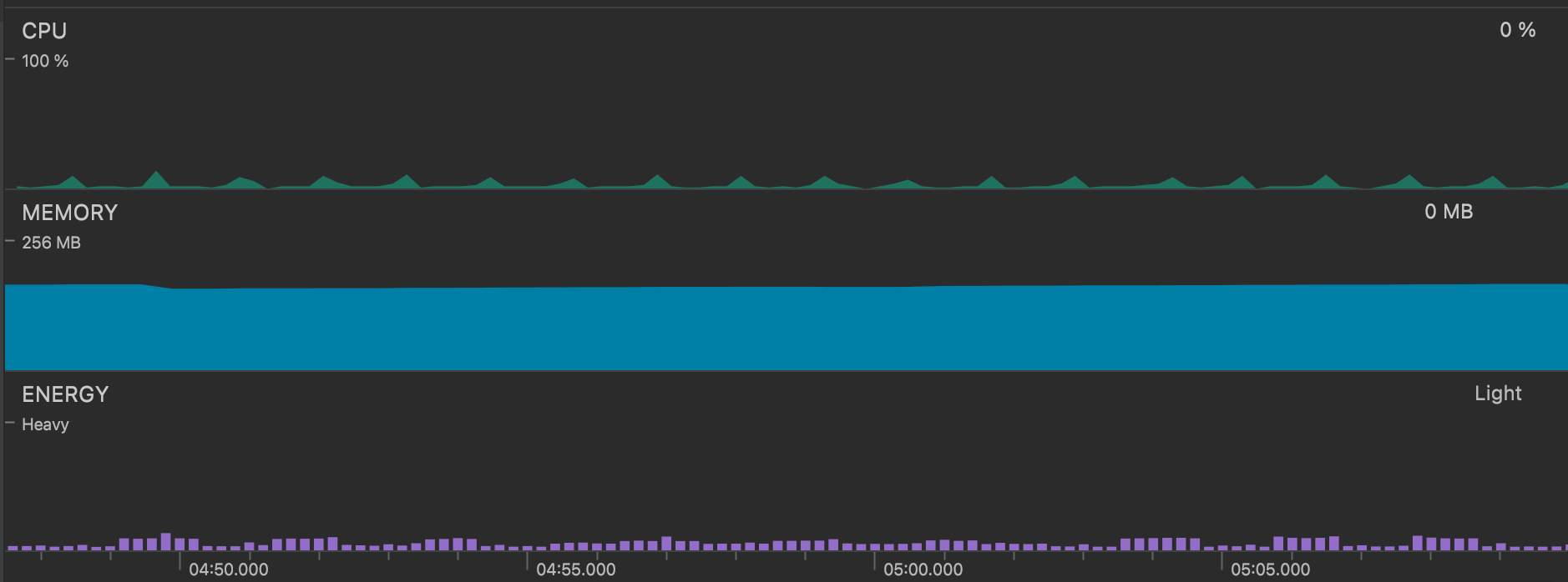
With hardware decoding comes battery life savings — essential for both today’s smartphones and tomorrow’s VR headsets. For example, a Google Pixel 6 with AV1 hardware decoding uses only minimal battery and CPU to decode and play our test video:

Bringing the best live video experience to Cloudflare Stream with AV1

AV1 encoding requires even more compute power

Just as decoding is significantly harder for end-user devices, it is also significantly harder to encode video using AV1. When AV1 was announced in 2018, many doubted whether hardware would be able to encode it efficiently enough for the protocol to be adopted quickly enough.

To demonstrate this, we encoded the 4K rendering of Big Buck Bunny (a classic among video engineers!) into AV1, using an AMD EPYC 7642 48-Core Processor with 256 GB RAM. This CPU continues to be a workhorse of our compute fleet, as we have written about previously. We used the following command to re-encode the video, based on the example in the ffmpeg AV1 documentation:

ffmpeg -i bbb_sunflower_2160p_30fps_normal.mp4 -c:v libaom-av1 -crf 30 -b:v 0 -strict -2 av1_test.mkv

Using a single core, encoding just two seconds of video at 30fps took over 30 minutes. Even if all 48 cores were used to encode, it would take at minimum over 43 seconds to encode just two seconds of video. Live encoding using only CPUs would require over 20 servers running at full capacity.

Special-purpose AV1 software encoders like rav1e and SVT-AV1 that run on general purpose CPUs can encode somewhat faster than libaom-av1 with ffmpeg, but still consume a huge amount of compute power to encode AV1 in real-time, requiring multiple servers running at full capacity in many scenarios.

Cloudflare Stream encodes your video to AV1 in real-time

At Cloudflare, we control both the hardware and software on our network. So to solve the CPU constraint, we’ve installed dedicated AV1 hardware encoders, designed specifically to encode AV1 at blazing fast speeds. This end to end control is what lets us encode your video to AV1 in real-time. This is entirely out of reach to most public cloud customers, including the video infrastructure providers who depend on them for compute power.

Encoding in real-time means you can use AV1 for live video streaming, where saving bandwidth matters most. With a pre-recorded video, the client video player can fetch future segments of video well in advance, relying on a buffer that can be many tens of seconds long. With live video, buffering is constrained by latency — it’s not possible to build up a large buffer when viewing a live stream. There is less margin for error with live streaming, and every byte saved means that if a viewer’s connection is interrupted, it takes less time to recover before the buffer is empty.

Stream lets you support AV1 with no additional work

AV1 has a chicken or the egg dilemma. And we’re helping solve it.

Companies with large video libraries often re-encode their entire content library to a new codec before using it. But AV1 is so computationally intensive that re-encoding whole libraries has been cost prohibitive. Companies have to choose specific videos to re-encode, and guess which content will be most viewed ahead of time. This is particularly challenging for apps with user generated content, where content can suddenly go viral, and viewer patterns are hard to anticipate.

This has slowed down the adoption of AV1 — content providers wait for more devices to support AV1, and device manufacturers wait for more content to use AV1. Which will come first?

With Cloudflare Stream there is no need to manually trigger re-encoding, re-upload video, or manage the bulk encoding of a large video library. This is a unique approach that is made possible by integrating encoding and delivery into a single product — it is not possible to encode on-demand using the old way of encoding first, and then pointing a CDN at a bucket of pre-encoded files.

We think this approach can accelerate the adoption of AV1. Consider a video app with millions of minutes of user-generated video. Most videos will never be watched again. In the old model, developers would have to spend huge sums of money to encode upfront, or pick and choose which videos to re-encode. With Stream, we can help anyone incrementally adopt AV1, without re-encoding upfront. As we work towards making AV1 Generally Available, we’ll be working to make supporting AV1 simple and painless, even for videos already uploaded to Stream, with no special configuration necessary.

Open, royalty-free, and widely supported

At Cloudflare, we are committed to open standards and fighting patent trolls. While there are multiple competing options for new video codecs, we chose to support AV1 first in part because it is open source and has royalty-free licensing.

Other encoding codecs force device manufacturers to pay royalty fees in order to adopt their standard in consumer hardware, and have been quick to file lawsuits against competing video codecs. The group behind the open and royalty-free VP8 and VP9 codecs have been pushing back against this model for more than a decade, and AV1 is the successor to these codecs, with support from all the biggest technology companies, both software and hardware. Beyond its technical accomplishments, AV1 is a clear message from the industry that the future of video encoding should be open, royalty-free, and free from patent litigation.

Try AV1 right now with your live stream or live recording

Support for AV1 is currently in open beta. You can try using AV1 on your own live video with Cloudflare Stream right now — just add the ?betaCodecSuggestion=av1 query parameter to the HLS or DASH manifest URL for any live stream or live recording created after October 1st in Cloudflare Stream. Read the docs to get started. If you don’t yet have a Cloudflare account, you can sign up here and start using Cloudflare Stream in just a few minutes.

We also have a recording of a live video, encoded using AV1, that you can watch here. Note that Safari does not yet support AV1.

We encourage you to try AV1 with your test streams, and we’d love your feedback. Join our Discord channel and tell us what you’re building, and what kinds of video you’re interested in using AV1 with. We’d love to hear from you!

Common streaming data enrichment patterns in Amazon Kinesis Data Analytics for Apache Flink

Post Syndicated from Ali Alemi original https://aws.amazon.com/blogs/big-data/common-streaming-data-enrichment-patterns-in-amazon-kinesis-data-analytics-for-apache-flink/

Stream data processing allows you to act on data in real time. Real-time data analytics can help you have on-time and optimized responses while improving overall customer experience.

Apache Flink is a distributed computation framework that allows for stateful real-time data processing. It provides a single set of APIs for building batch and streaming jobs, making it easy for developers to work with bounded and unbounded data. Apache Flink provides different levels of abstraction to cover a variety of event processing use cases.

Amazon Kinesis Data Analytics is an AWS service that provides a serverless infrastructure for running Apache Flink applications. This makes it easy for developers to build highly available, fault tolerant, and scalable Apache Flink applications without needing to become an expert in building, configuring, and maintaining Apache Flink clusters on AWS.

Data streaming workloads often require data in the stream to be enriched via external sources (such as databases or other data streams). For example, assume you are receiving coordinates data from a GPS device and need to understand how these coordinates map with physical geographic locations; you need to enrich it with geolocation data. You can use several approaches to enrich your real-time data in Kinesis Data Analytics depending on your use case and Apache Flink abstraction level. Each method has different effects on the throughput, network traffic, and CPU (or memory) utilization. In this post, we cover these approaches and discuss their benefits and drawbacks.

Data enrichment patterns

Data enrichment is a process that appends additional context and enhances the collected data. The additional data often is collected from a variety of sources. The format and the frequency of the data updates could range from once in a month to many times in a second. The following table shows a few examples of different sources, formats, and update frequency.

Data Format Update Frequency
IP address ranges by country CSV Once a month
Company organization chart JSON Twice a year
Machine names by ID CSV Once a day
Employee information Table (Relational database) A few times a day
Customer information Table (Non-relational database) A few times an hour
Customer orders Table (Relational database) Many times a second

Based on the use case, your data enrichment application may have different requirements in terms of latency, throughput, or other factors. The remainder of the post dives deeper into different patterns of data enrichment in Kinesis Data Analytics, which are listed in the following table with their key characteristics. You can choose the best pattern based on the trade-off of these characteristics.

Enrichment Pattern Latency Throughput Accuracy if Reference Data Changes Memory Utilization Complexity
Pre-load reference data in Apache Flink Task Manager memory Low High Low High Low
Partitioned pre-loading of reference data in Apache Flink state Low High Low Low Low
Periodic Partitioned pre-loading of reference data in Apache Flink state Low High Medium Low Medium
Per-record asynchronous lookup with unordered map Medium Medium High Low Low
Per-record asynchronous lookup from an external cache system Low or Medium (Depending on Cache storage and implementation) Medium High Low Medium
Enriching streams using the Table API Low High High Low – Medium (depending on the selected join operator) Low

Enrich streaming data by pre-loading the reference data

When the reference data is small in size and static in nature (for example, country data including country code and country name), it’s recommended to enrich your streaming data by pre-loading the reference data, which you can do in several ways.

To see the code implementation for pre-loading reference data in various ways, refer to the GitHub repo. Follow the instructions in the GitHub repository to run the code and understand the data model.

Pre-loading of reference data in Apache Flink Task Manager memory

The simplest and also fastest enrichment method is to load the enrichment data into each of the Apache Flink task managers’ on-heap memory. To implement this method, you create a new class by extending the RichFlatMapFunction abstract class. You define a global static variable in your class definition. The variable could be of any type, the only limitation is that it should extend java.io.Serializable—for example, java.util.HashMap. Within the open() method, you define a logic that loads the static data into your defined variable. The open() method is always called first, during the initialization of each task in Apache Flink’s task managers, which makes sure the whole reference data is loaded before the processing begins. You implement your processing logic by overriding the processElement() method. You implement your processing logic and access the reference data by its key from the defined global variable.

The following architecture diagram shows the full reference data load in each task slot of the task manager.

diagram shows the full reference data load in each task slot of the task manager.

This method has the following benefits:

  • Easy to implement
  • Low latency
  • Can support high throughput

However, it has the following disadvantages:

  • If the reference data is large in size, the Apache Flink task manager may run out of memory.
  • Reference data can become stale over a period of time.
  • Multiple copies of the same reference data are loaded in each task slot of the task manager.
  • Reference data should be small to fit in the memory allocated to a single task slot. In Kinesis Data Analytics, each Kinesis Processing Unit (KPU) has 4 GB of memory, out of which 3 GB can be used for heap memory. If ParallelismPerKPU in Kinesis Data Analytics is set to 1, one task slot runs in each task manager, and the task slot can use the whole 3 GB of heap memory. If ParallelismPerKPU is set to a value greater than 1, the 3 GB of heap memory is distributed across multiple task slots in the task manager. If you’re deploying Apache Flink in Amazon EMR or in a self-managed mode, you can tune taskmanager.memory.task.heap.size to increase the heap memory of a task manager.

Partitioned pre-loading of reference data in Apache Flink State

In this approach, the reference data is loaded and kept in the Apache Flink state store at the start of the Apache Flink application. To optimize the memory utilization, first the main data stream is divided by a specified field via the keyBy() operator across all task slots. Furthermore, only the portion of the reference data that corresponds to each task slot is loaded in the state store.

This is achieved in Apache Flink by creating the class PartitionPreLoadEnrichmentData, extending the RichFlatMapFunction abstract class. Within the open method, you override the ValueStateDescriptor method to create a state handle. In the referenced example, the descriptor is named locationRefData, the state key type is String, and the value type is Location. In this code, we use ValueState compared to MapState because we only hold the location reference data for a particular key. For example, when we query Amazon S3 to get the location reference data, we query for the specific role and get a particular location as a value.

In Apache Flink, ValueState is used to hold a specific value for a key, whereas MapState is used to hold a combination of key-value pairs.

This technique is useful when you have a large static dataset that is difficult to fit in memory as a whole for each partition.

The following architecture diagram shows the load of reference data for the specific key for each partition of the stream.

diagram shows the load of reference data for the specific key for each partition of the stream.

For example, our reference data in the sample GitHub code has roles which are mapped to each building. Because the stream is partitioned by roles, only the specific building information per role is required to be loaded for each partition as the reference data.

This method has the following benefits:

  • Low latency.
  • Can support high throughput.
  • Reference data for specific partition is loaded in the keyed state.
  • In Kinesis Data Analytics, the default state store configured is RocksDB. RocksDB can utilize a significant portion of 1 GB of managed memory and 50 GB of disk space provided by each KPU. This provides enough room for the reference data to grow.

However, it has the following disadvantages:

  • Reference data can become stale over a period of time

Periodic partitioned pre-loading of reference data in Apache Flink State

This approach is a fine-tune of the previous technique, where each partitioned reference data is reloaded on a periodic basis to refresh the reference data. This is useful if your reference data changes occasionally.

The following architecture diagram shows the periodic load of reference data for the specific key for each partition of the stream.

diagram shows the periodic load of reference data for the specific key for each partition of the stream.

In this approach, the class PeriodicPerPartitionLoadEnrichmentData is created, extending the KeyedProcessFunction class. Similar to the previous pattern, in the context of the GitHub example, ValueState is recommended here because each partition only loads a single value for the key. In the same way as mentioned earlier, in the open method, you define the ValueStateDescriptor to handle the value state and define a runtime context to access the state.

Within the processElement method, load the value state and attach the reference data (in the referenced GitHub example, buildingNo to the customer data). Also register a timer service to be invoked when the processing time passes the given time. In the sample code, the timer service is scheduled to be invoked periodically (for example, every 60 seconds). In the onTimer method, update the state by making a call to reload the reference data for the specific role.

This method has the following benefits:

  • Low latency.
  • Can support high throughput.
  • Reference data for specific partitions is loaded in the keyed state.
  • Reference data is refreshed periodically.
  • In Kinesis Data Analytics, the default state store configured is RocksDB. Also, 50 GB of disk space provided by each KPU. This provides enough room for the reference data to grow.

However, it has the following disadvantages:

  • If the reference data changes frequently, the application still has stale data depending on how frequently the state is reloaded
  • The application can face load spikes during reload of reference data

Enrich streaming data using per-record lookup

Although pre-loading of reference data provides low latency and high throughput, it may not be suitable for certain types of workloads, such as the following:

  • Reference data updates with high frequency
  • Apache Flink needs to make an external call to compute the business logic
  • Accuracy of the output is important and the application shouldn’t use stale data

Normally, for these types of use cases, developers trade-off high throughput and low latency for data accuracy. In this section, you learn about a few of common implementations for per-record data enrichment and their benefits and disadvantages.

Per-record asynchronous lookup with unordered map

In a synchronous per-record lookup implementation, the Apache Flink application has to wait until it receives the response after sending every request. This causes the processor to stay idle for a significant period of processing time. Instead, the application can send a request for other elements in the stream while it waits for the response for the first element. This way, the wait time is amortized across multiple requests and therefore it increases the process throughput. Apache Flink provides asynchronous I/O for external data access. While using this pattern, you have to decide between unorderedWait (where it emits the result to the next operator as soon as the response is received, disregarding the order of the element on the stream) and orderedWait (where it waits until all inflight I/O operations complete, then sends the results to the next operator in the same order as original elements were placed on the stream). Usually, when downstream consumers disregard the order of the elements in the stream, unorderedWait provides better throughput and less idle time. Visit Enrich your data stream asynchronously using Kinesis Data Analytics for Apache Flink to learn more about this pattern.

The following architecture diagram shows how an Apache Flink application on Kinesis Data Analytics does asynchronous calls to an external database engine (for example Amazon DynamoDB) for every event in the main stream.

diagram shows how an Apache Flink application on Kinesis Data Analytics does asynchronous calls to an external database engine (for example Amazon DynamoDB) for every event in the main stream.

This method has the following benefits:

  • Still reasonably simple and easy to implement
  • Reads the most up-to-date reference data

However, it has the following disadvantages:

  • It generates a heavy read load for the external system (for example, a database engine or an external API) that hosts the reference data
  • Overall, it might not be suitable for systems that require high throughput with low latency

Per-record asynchronous lookup from an external cache system

A way to enhance the previous pattern is to use a cache system to enhance the read time for every lookup I/O call. You can use Amazon ElastiCache for caching, which accelerates application and database performance, or as a primary data store for use cases that don’t require durability like session stores, gaming leaderboards, streaming, and analytics. ElastiCache is compatible with Redis and Memcached.

For this pattern to work, you must implement a caching pattern for populating data in the cache storage. You can choose between a proactive or reactive approach depending your application objectives and latency requirements. For more information, refer to Caching patterns.

The following architecture diagram shows how an Apache Flink application calls to read the reference data from an external cache storage (for example, Amazon ElastiCache for Redis). Data changes must be replicated from the main database (for example, Amazon Aurora) to the cache storage by implementing one of the caching patterns.

diagram shows how an Apache Flink application calls to read the reference data from an external cache storage (for example, Amazon ElastiCache for Redis). Data changes must be replicated from the main database (for example, Amazon Aurora) to the cache storage by implementing one of the caching patterns.

Implementation for this data enrichment pattern is similar to the per-record asynchronous lookup pattern; the only difference is that the Apache Flink application makes a connection to the cache storage, instead of connecting to the primary database.

This method has the following benefits:

  • Better throughput because caching can accelerate application and database performance
  • Protects the primary data source from the read traffic created by the stream processing application
  • Can provide lower read latency for every lookup call
  • Overall, might not be suitable for medium to high throughput systems that want to improve data freshness

However, it has the following disadvantages:

  • Additional complexity of implementing a cache pattern for populating and syncing the data between the primary database and the cache storage
  • There is a chance for the Apache Flink stream processing application to read stale reference data depending on what caching pattern is implemented
  • Depending on the chosen cache pattern (proactive or reactive), the response time for each enrichment I/O may differ, therefore the overall processing time of the stream could be unpredictable

Alternatively, you can avoid these complexities by using the Apache Flink JDBC connector for Flink SQL APIs. We discuss enrichment stream data via Flink SQL APIs in more detail later in this post.

Enrich stream data via another stream

In this pattern, the data in the main stream is enriched with the reference data in another data stream. This pattern is good for use cases in which the reference data is updated frequently and it’s possible to perform change data capture (CDC) and publish the events to a data streaming service such as Apache Kafka or Amazon Kinesis Data Streams. This pattern is useful in the following use cases, for example:

  • Customer purchase orders are published to a Kinesis data stream, and then join with customer billing information in a DynamoDB stream
  • Data events captured from IoT devices should enrich with reference data in a table in Amazon Relational Database Service (Amazon RDS)
  • Network log events should enrich with the machine name on the source (and the destination) IP addresses

The following architecture diagram shows how an Apache Flink application on Kinesis Data Analytics joins data in the main stream with the CDC data in a DynamoDB stream.

diagram shows how an Apache Flink application on Kinesis Data Analytics joins data in the main stream with the CDC data in a DynamoDB stream.

To enrich streaming data from another stream, we use a common stream to stream join patterns, which we explain in the following sections.

Enrich streams using the Table API

Apache Flink Table APIs provide higher abstraction for working with data events. With Table APIs, you can define your data stream as a table and attach the data schema to it.

In this pattern, you define tables for each data stream and then join those tables to achieve the data enrichment goals. Apache Flink Table APIs support different types of join conditions, like inner join and outer join. However, you want to avoid those if you’re dealing with unbounded streams because those are resource intensive. To limit the resource utilization and run joins effectively, you should use either interval or temporal joins. An interval join requires one equi-join predicate and a join condition that bounds the time on both sides. To better understand how to implement an interval join, refer to Get started with Apache Flink SQL APIs in Kinesis Data Analytics Studio.

Compared to interval joins, temporal table joins don’t work with a time period within which different versions of a record are kept. Records from the main stream are always joined with the corresponding version of the reference data at the time specified by the watermark. Therefore, fewer versions of the reference data remain in the state.

Note that the reference data may or may not have a time element associated with it. If it doesn’t, you may need to add a processing time element for the join with the time-based stream.

In the following example code snippet, the update_time column is added to the currency_rates reference table from the change data capture metadata such as Debezium. Furthermore, it’s used to define a watermark strategy for the table.

CREATE TABLE currency_rates (
    currency STRING,
    conversion_rate DECIMAL(32, 2),
    update_time TIMESTAMP(3) METADATA FROM `values.source.timestamp` VIRTUAL,
        WATERMARK FOR update_time AS update_time,
    PRIMARY KEY(currency) NOT ENFORCED
) WITH (
   'connector' = 'kafka',
   'value.format' = 'debezium-json',
   /* ... */
);

This method has the following benefits:
  • Easy to implement
  • Low latency
  • Can support high throughput when reference data is a data stream

SQL APIs provide higher abstractions over how the data is processed. For more complex logic around how the join operator should process, we recommend you always start with SQL APIs first and use DataStream APIs if you really need to.

Conclusion

In this post, we demonstrated different data enrichment patterns in Kinesis Data Analytics. You can use these patterns and find the one that addresses your needs and quickly develop a stream processing application.

For further reading on Kinesis Data Analytics, visit the official product page.


About the Authors

About the author Ali AlemiAli Alemi is a Streaming Specialist Solutions Architect at AWS. Ali advises AWS customers with architectural best practices and helps them design real-time analytics data systems that are reliable, secure, efficient, and cost-effective. He works backward from customers’ use cases and designs data solutions to solve their business problems. Prior to joining AWS, Ali supported several public sector customers and AWS consulting partners in their application modernization journey and migration to the cloud.

About the author Subham RakshitSubham Rakshit is a Streaming Specialist Solutions Architect for Analytics at AWS based in the UK. He works with customers to design and build search and streaming data platforms that help them achieve their business objective. Outside of work, he enjoys spending time solving jigsaw puzzles with his daughter.

About the author Dr. Sam MokhtariDr. Sam Mokhtari is a Senior Solutions Architect in AWS. His main area of depth is data and analytics, and he has published more than 30 influential articles in this field. He is also a respected data and analytics advisor who led several large-scale implementation projects across different industries, including energy, health, telecom, and transport.

The Storage Pod Story: Innovation to Commodity

Post Syndicated from original https://www.backblaze.com/blog/the-storage-pod-story-innovation-to-commodity/

It has been over six years since we released Storage Pod 6.0. Yes, we have improved that system since then, several times. We’ve added more memory, upgraded the CPU, and of course deployed larger disks. I suppose we could have written blog posts about those improvements, a Storage Pod 6.X post or two or three, but somehow that felt a bit hollow.

About 18 months ago, we talked about The Next Backblaze Storage Pod. We had started using Dell servers in our Amsterdam data center, although we were still building and deploying the version 6.X storage pods in our U.S. data centers. That changed about six months ago and we haven’t built or deployed a Backblaze Storage Pod since that time. Here’s what we’ve done instead.

A Backblaze-Worthy Storage Server

In September of 2019, we wrote a blog post to celebrate the 10 year anniversary of open sourcing our Storage Pod design. In that post we mused about the build/buy decision and stated the criteria we needed to consider if we were going to buy storage servers from someone else: cost, ease of maintenance, the use of commodity parts, ability to scale production, and so on. Also in that post, we compiled a list of storage servers on the market at the time which were similar to our Storage Pod design.

We then proceeded to test several different storage servers from the list and elsewhere. The testing was done over a period of about a year using the criteria noted earlier. The process progressed and one server, a 60-drive Supermicro server, was selected to move on to the next stage, production performance testing.

Here we would observe the server’s performance and test its compatibility with our operational architecture. We built a vault of 20 Supermicro servers and placed it into production, and at the same time we placed a standard Storage Pod vault into production. The two vaults ran the same software and we would track each vault’s performance throughout.

When a Backblaze Vault enters production, 60 tomes of storage come online at the same time joining thousands of other tomes ready to receive data. Each vault has the same opportunity to load data, but this will vary depending on the performance of the vault to process the requests received. In general, the more performant the vault, the more data it can upload each day.

The comparison of how much data each vault uploaded each day is shown below. Vault 1084 is composed of 20 Supermicro servers and Vault 1085 is composed of 20 Backblaze Storage Pods.

The Supermicro vault (1084) started with a limit of 2,500 simultaneous connections allowed for the first seven days. Once that limit was lifted and both vaults were set to 5,000 simultaneous connections, the Supermicro vault generally outperformed the Backblaze vault over the remainder of the observation period.

What happened to the data once the test was over? It stayed in the Supermicro vault and that vault became a permanent part of our production environment. It is still in operation today, joined by over 1,100 additional Supermicro servers. Safe to say, we moved ahead with using the Supermicro servers in our environment in place of building new Storage Pods.

The Server Model We Use

The Supermicro model we order from Supermicro is the PIO-5049P-E1CR60L (PIO-5049). That model is not sold via the Supermicro website. That said, model SSG-6049P-E1CR60L (SSG-6049) is similar and is widely available. Both models have 60 drives, but the chassis is slightly different, and the motherboards are different with the PIO-5049 model having a single CPU slot, and the SSG-6049 model having two CPU slots. Let’s compare the basics of the two models below.

In practice, the Supermicro SSG-6049 model supports newer components such as the latest CPUs and allows more memory versus the Supermicro PIO-5049 model, but the latter is more than capable of supporting our needs.

Can You Build It?

A little over 13 years ago, we wrote the Petabytes on a Budget blog post introducing Backblaze Storage Pods to the world and open sourcing the design. Since then, many individuals, organizations, and businesses have taken the various storage pod designs we published over the years and built their own storage servers. That’s awesome.

We know building a Storage Pod was not easy. Oh, the assembly was simple enough, but getting all the parts you needed was a challenge: searching endlessly for 5-port backplanes (minimum order quantity 1,000-ouch, sorry) or having to build your own power supply cables. While many of you enjoyed the challenge; many didn’t.
For the Supermicro system, let’s work with the Supermicro SSG-6049 model as it is available to everyone and see what it would take for you to acquire/assemble/build a single Supermicro storage server.

Option One: Go Standard

The easiest thing to do is to order a pre-configured SSG-6049 model from Supermicro or you can try one of their online reseller sites such as Canada Computers & Electronics or ComputerLink, which offer the same “complete system”. In these cases, the ability to customize the server is minimal and requires direct contact with the vendor for most changes. If that works for you, then you’re all set.

Option Two: Configure

If you want to design your own system you can try Supermicro resellers such as IT Creations (US) and Server Simply (EU) which have configurators that allow you to select your CPU, motherboard, network cards, memory, and various other components. This is a great option but given the number of different options and the possibility of incompatibilities between components, you need to be careful here. Don’t rely on the configurator to catch a component mismatch.

Option Three: Create

Here you might buy the most stripped-down server you can find and replace nearly everything inside—motherboard, CPU, fans, switches, cables and so on. You’ll probably void any warranty you had on the system, but we suspect you knew that already. Regardless, you can take the base system and stuff it full of smoking-fast everything so that your copy of “Ferris Buellers Day Off” downloads in picoseconds. That’s the fun part of building your own storage server, when you are done it is uniquely yours.

Which option you choose is, of course, your choice, and while ordering a standard system from Supermicro may not be as satisfying as soldering heat sinks to the motherboard or neatly tying off your SATA cable runs, it will give you more time to watch Ferris, so there’s that.

FYI, Supermicro has an extensive network of resellers around the world. While the options above fall neatly into three categories, each reseller has their own way of working with their clients. If you are going to buy or build your own Supermicro storage server or have already done so, share your experience with your colleagues in the comments below or on your favorite forum or community site.

What About Pricing

Supermicro does not publish prices and we are not going to out them here, but we wanted to see if we could determine the street price for the Supermicro SSG-6049 system by surveying reseller websites. It was not pretty. In our research, we saw prices for the Supermicro SSG-6049 model range from $6K to 40K on different reseller sites. On the website with the $6K price they started with a fictitious base system that you could not order, and then listed the various components you were required to add, such as CPU, memory, hard drives, etc. At the $40K website the reseller didn’t bother to list any of the components; it just had the model and the price—no specs or technical information. Classic buyer beware scenarios in both cases.

The other variable that made the street price hard to determine was that resellers often bundled other services into the price of the system such as installation, annual maintenance, and even shipping. All are reasonable services for a reseller to offer, but they cloud the picture when trying to determine the actual cost of the product you are trying to buy. At best, we can say that the street price is somewhere between $20K and $30K, but we are not very confident with that range.

Storage Server Pricing Over Time

Since 2009 we have tracked the cost per GB of each Storage Pod version we have produced. We’ve updated the chart below to add both Storage Pod version 6.X, our most current Storage Pod configuration, and the Supermicro storage server we are buying, model PIO-5049.

The cost per GB is computed by taking the total hardware cost of a storage server, including the hard drives, and dividing by the total storage in the server at the time. When Storage Pod 1.0 was released in September 2009, the system cost was about $0.12/GB, and as you can see that has decreased over time to $0.02/GB in the Supermicro systems.

One point to note is that both the Storage Pod 6.X ($0.028/GB) and Supermicro ($0.020/GB) servers use the same 16TB hard drive models. We believe the difference between the cost per GB of the two cohorts ($0.008) is primarily based on the operational efficiency obtained by Supermicro in making and selling tens of thousands of units a month versus Backblaze assembling a hundred 6.X Storage Pods on our own. In other words, Supermicro’s scale of production has enabled us to get performant systems for less than if we continued to build them ourselves.

What’s Next for Storage Pods

No one here at Backblaze is ready to write the obituary for our beloved red Backblaze Storage Pods. Afterall, the innovation that was the Storage Pod created the opportunity for Backblaze to change the dynamics of the storage market. Now that the Storage Pod hardware has been commoditized, our cloud storage software platform is what enables us to continue to deliver value to businesses and individuals alike.

All that means is that our next Storage Pod probably won’t be an incremental change, but instead something completely new, at least for us. It may not even be a Storage Pod—who knows? That said, we will continue to upgrade our existing Storage Pods with new CPUs, memory, and such, and they’ll be around for years to come. At which point we may give them away or crush them (again). In the meantime, we’ll probably do another blog post or two so we can post a few pictures and tell a few stories. Or maybe we’ll just move on. Hard to say right now.

Thanks to all our Storage Pod readers for your comments and suggestions over the years. You’ve made us better along the way and we look forward to continuing to hear from you as our journey continues.

The post The Storage Pod Story: Innovation to Commodity appeared first on Backblaze Blog | Cloud Storage & Cloud Backup.

GitHub Availability Report: September 2022

Post Syndicated from Jakub Oleksy original https://github.blog/2022-10-05-github-availability-report-september-2022/

In September, we experienced one incident that resulted in significant impact and degraded state of availability to multiple GitHub services. We also experienced one incident resulting in significant impact to Codespaces. We are still investigating that incident and will include it in next month’s report. This report also sheds light into an incident that impacted Codespaces in August and an incident that impacted GitHub Actions in August.

September 8 19:44 UTC (lasting 5 hours and 11 minutes)

On September 8, 2022 at 19:44 UTC, our monitoring detected an increase in the number of pull request merge failures. The impact was concentrated on Enterprise Managed Users (EMUs) with a small number of bot accounts also affected.

Within 45 minutes, we traced the cause to a data transition that removed inconsistent data from profile records. Unfortunately, the transition incorrectly operated on EMU accounts, removing some data that is required to successfully merge pull requests via the UI and our API. CLI merges were unaffected.

We restored the data from backup, but this took longer than we had anticipated. We simultaneously pursued a workaround in code, but opted not to proceed with it as it could introduce data inconsistencies. Our restore operation resolved the issue with our pull request monitors having recovered by September 9, 2022 at 00:55 UTC.

Following this incident, we have made changes to our data transition procedures to allow for faster restores and transitions that can be automatically rolled back without relying on backups. We are also working on multiple improvements to our testing processes as they relate to EMUs.

September 28 03:53 UTC (lasting 1 hour and 16 minutes)

Our alerting systems detected an incident that impacted most Codespaces customers. Due to the recency of this incident, we are still investigating the contributing factors and will provide a more detailed update on cause and remediation in the October Availability Report, which we will publish the first Wednesday of November.

Follow up to August 29 12:51 UTC (lasting 5 hours and 40 minutes)

On August 29, 2022 at 12:51 UTC, our monitoring detected an increase in Codespaces create and start errors. We also started seeing DNS-related networking errors in some running Codespaces where outbound DNS resolutions were failing. At 14:19 UTC, we updated the status for Codespaces from yellow to red due to broad user impact.

This incident was caused by an Ubuntu security patch in systemd that broke DNS resolution. In recent versions of Ubuntu, unattended upgrades for security fixes are enabled by default. Codespaces host VMs were using the default recommended settings to apply security patches automatically on running VMs. When this patch was published, Codespaces host VMs started installing and applying the patch after the VM was created. Once the patch was installed on a VM, DNS resolution was broken. Depending on the timing of when the patch was installed on the host VM, this led to a few different failure modes, including failure creating/starting Codespaces or failure, making outbound network calls inside of a codespace that was already running.

Once we identified systemd’s DNS resolver configuration as the source of these errors, we were able to mitigate the issue by disabling systemd’s DNS resolver and manually configuring an upstream DNS resolver IP address. We deployed a change to the DNS configuration on the host VMs at 18:13 UTC. By 18:21 UTC, we started seeing positive signs of recovery in our metrics and changed the status to yellow. Ten minutes later, at 18:31 UTC, all metrics were fully healthy and the incident was resolved.

Following this incident, we are updating our DNS configuration to reduce dependencies on systemd’s DNS resolver. We are also investigating whether we should continue to use unattended upgrades for security patches. Disabling unattended upgrades will give us more deterministic behavior at runtime, preventing external changes from breaking Codespaces. We will remain fully capable of quickly patching VMs across our fleet even with unattended upgrades disabled.

Follow up to August 18 14:33 UTC (lasting 3 hours and 23 minutes)

This incident occurred in August but was left out of the August report because it did not result in a widespread outage. Several GitHub Actions customers experienced issues because of the degradation so we decided to include it retroactively.

At 14:13 UTC, there was a sudden spike in traffic to GitHub Actions which resulted in a higher than usual write load on our services. A majority of our services handled this graciously, but one of our internal services that is used for generating security tokens started returning 503 Service Unavailable errors to requests, triggering an alert to the engineering team. Further investigation revealed that the token database was experiencing a performance degradation which, compounded by the increased load, caused us to hit the database’s max concurrent connections limit. This was made worse due to a mismatch between our client-side throttling limits and database capacity, which resulted in our throttling thresholds allowing more traffic than this database had capacity to handle.

We mitigated the issue by scaling up the impacted database while also allowing a higher number of concurrent connections to it. The impacted service went back to a healthy state and the incident was considered resolved at 17:36 UTC. In addition to the immediate actions, we have improved our monitoring and alerting to allow faster remediation. We are also evaluating changes to our throttling mechanisms to better account for this traffic pattern.

In summary

Please follow our status page for real-time updates on status changes. To learn more about what we’re working on, check out the GitHub Engineering Blog.

The Thorny Problem of Keeping the Internet’s Time (New Yorker)

Post Syndicated from original https://lwn.net/Articles/910418/

The New Yorker has a
lengthy article
on the Network Time Protocol and its creator David
Mills.

Coders sometimes joke, morbidly, about the “bus factor.” How many
people need to get hit by a bus before a given project is
endangered? It’s difficult to determine the bus factor for N.T.P.,
and time synchronization more broadly, especially now that
companies such as Google have developed their own N.T.P.-inspired
proprietary code. But it seems reasonable to say that N.T.P.’s bus
factor is rather small.

Al-Qudsi: Implementing truly safe semaphores in rust

Post Syndicated from original https://lwn.net/Articles/910417/

Mahmoud Al-Qudsi provides
extensive details
on what it takes to implement a safe semaphore type
in the Rust language.

The problem is that with n > 1, there’s no concept of a
“privileged” owning thread and all threads that have “obtained” the
semaphore do so equally. Therefore, a rust semaphore can only ever
provide read-only (&T) access to an underlying resource,
limiting the usefulness of such a semaphore almost to the point of
having no utility. As such, the only safe “owning” semaphore with
read-write access that can exist in the rust world would be
Semaphore<()>, or one that actually owns no data and can
only be used for its side effect of limiting concurrency while the
semaphore is “owned,” so to speak.

Announcing server-side encryption with Amazon Simple Queue Service -managed encryption keys (SSE-SQS) by default

Post Syndicated from James Beswick original https://aws.amazon.com/blogs/compute/announcing-server-side-encryption-with-amazon-simple-queue-service-managed-encryption-keys-sse-sqs-by-default/

This post is written by Sofiya Muzychko (Sr Product Manager), Nipun Chagari (Principal Solutions Architect), and Hardik Vasa (Senior Solutions Architect).

Amazon Simple Queue Service (SQS) now provides server-side encryption (SSE) using SQS-owned encryption (SSE-SQS) by default. This feature further simplifies the security posture to encrypt the message body in SQS queues.

SQS is a fully managed message queuing service that enables you to decouple and scale microservices, distributed systems, and serverless applications. Customers are increasingly decoupling their monolithic applications to microservices and moving sensitive workloads to SQS, such as financial and healthcare applications, whose compliance regulations mandate data encryption.

SQS already supports server-side encryption with customer-provided encryption keys using the AWS Key Management Service (SSE-KMS) or using SQS-owned encryption keys (SSE-SQS). Both encryption options greatly reduce the operational burden and complexity involved in protecting data. Additionally, with the SSE-SQS encryption type, you do not need to create, manage, or pay for SQS-managed encryption keys.

Using the default encryption

With this feature, all newly created queues using HTTPS (TLS) and Signature Version 4 endpoints are encrypted using SQS-owned encryption (SSE-SQS) by default, enhancing the protection of your data against unauthorized access. Any new queue created using the non-TLS endpoint will not enable SSE-SQS encryption by default. We hence encourage you to create SQS queues using HTTPS endpoints as a security best practice.

The SSE-SQS default encryption is available for both standard and FIFO. You do not need to make any code or application changes to encrypt new queues. This does not affect existing queues. You can however change the encryption option for existing queues at any time using the SQS console, AWS Command Line Interface, or API.

Create queue

The preceding image shows the SQS queue creation console wizard with configuration options for encryption. As you can see, server-side encryption is enabled by default with encryption key type SSE-SQS option selected.

Creating a new SQS queue with SSE-SQS encryption using AWS CloudFormation

Default SSE-SQS encryption is also supported in AWS CloudFormation. To learn more, see this documentation page.

Here is the sample CloudFormation template to create an SQS standard queue with SQS owned Server Side Encryption (SSE-SQS) explicitly enabled.

AWSTemplateFormatVersion: "2010-09-09"
Description: SSE-SQS Cloudformation template
Resources:
  SQSEncryptionQueue:
    Type: AWS::SQS::Queue
    Properties: 
      MaximumMessageSize: 262144
      MessageRetentionPeriod: 86400
      QueueName: SSESQSQueue
      SqsManagedSseEnabled: true
      KmsDataKeyReusePeriodSeconds: 900
      VisibilityTimeout: 30

Note that if the SqsManagedSseEnabled: true property is not specified, SSE-SQS is enabled by default.

Configuring SSE-SQS encryption for existing queues vis AWS Management Console

To configure SSE-SQS encryption for an existing queue using the SQS console:

  1. Navigate to the SQS console at https://console.aws.amazon.com/sqs/.
  2. In the navigation pane, choose Queues.
  3. Select a queue, and then choose Edit.
  4. Under the Encryption dialog box, for Server-side encryption, choose Enabled.
  5. Select Amazon SQS key (SSE-SQS).
  6. Choose Save.

Edit standard queue

To configure SSE-SQS encryption for an existing queue using the AWS CLI

To enable SSE-SQS to an existing queue with no encryption, use the following AWS CLI command

aws sqs set-queue-attributes --queue-url <queueURL> --attributes SqsManagedSseEnabled=true

Replace <queueURL> with the URL of your SQS queue.

To disable SSE-SQS for an existing queue using the AWS CLI, run:

aws sqs set-queue-attributes --queue-url <queueURL> --attributes SqsManagedSseEnabled=false

Testing the queue with the SSE-SQS encryption enabled

To test sending message to the SQS queue with SSE-SQS enabled, run:

aws sqs send-message --queue-url <queueURL> --message-body test-message

Replace <queueURL> with the URL of your SQS queue. You see the following response, which means the message is successfully sent to the queue:

{
    "MD5OfMessageBody": "beaa0032306f083e847cbf86a09ba9b2",
    "MessageId": "6e53de76-7865-4c45-a640-f058c24a619b"
}

Default SSE-SQS encryption key rotation

You can choose how often the keys will be rotated by configuring the KmsDataKeyReusePeriodSeconds queue attribute. The value must be an integer between 60 (1 minute) and 86,400 (24 hours). The default is 300 (5 minutes).

To update the KMS data key reuse period for an existing SQS queue, run:

aws sqs set-queue-attributes --queue-url <queueURL> --attributes KmsDataKeyReusePeriodSeconds=900

This configures the queue with KMS key rotation to every 900 seconds (15 minutes).

Default SSE-SQS and encrypted messages

Encrypting a message makes its contents unavailable to unauthorized or anonymous users. Anonymous requests are requests made to a queue that is open to a public network without any authentication. Note, if you are using anonymous SendMessage and ReceiveMessage requests to the newly created queues, the requests will now be rejected with SSE-SQS enabled by default.

Making anonymous requests to SQS queues does not follow SQS security best practices. We strongly recommend updating your policy to make signed requests to SQS queues using AWS SDK or AWS CLI and to continue using SSE-SQS enabled by default.

Look at the SQS service response for anonymous messages when SSE-SQS encryption is enabled. For an existing queue, you can change the queue policy to grant all users (anonymous users) SendMessage permission for a queue named EncryptionQueue:

{
  "Version": "2012-10-17",
  "Id": "Queue1_Policy_UUID",
  "Statement": [
    {
      "Sid": "Queue1_SendMessage",
      "Effect": "Allow",
      "Principal": "*",
      "Action": "sqs:SendMessage",
      "Resource": "<queueARN>"
    }
  ]
}

You can then make an anonymous request against the queue:

curl <queueURL> -d 'Action=SendMessage&MessageBody=Hello'

You get an error message similar to the following:

<?xml version="1.0"?>
<ErrorResponse
	xmlns="http://queue.amazonaws.com/doc/2012-11-05/">
	<Error>
		<Type>Sender</Type>
		<Code>AccessDenied</Code>
		<Message>Access to the resource The specified queue does not exist or you do not have access to it. is denied.</Message>
		<Detail/>
	</Error>
	<RequestId> RequestID </RequestId>
</ErrorResponse>

However, for any reason if you want to continue using anonymous requests to the newly created queues in the future, you must create or update the queue with SSE-SQS encryption disabled.

SqsManagedSseEnabled=false

You can also disable the SSE-SQS using the Amazon SQS console.

Encrypting SQS queues with your own encryption keys

You can always change the default of SSE-SQS queues encryption and use your own keys. To encrypt SQS queues with your own encryption keys using the AWS Key Management Service (SSE-KMS), the default encryption with SSE-SQS can be overwritten to SSE-KMS during the queue creation process or afterwards.

You can update the SQS queue Server-side encryption key type using the Amazon SQS console, AWS Command Line Interface, or API.

Benefits of SQS owned encryption (SSE-SQS)

There are a number of significant benefits to encrypting your data with SQS owned encryption (SSE-SQS):

  • SSE-SQS lets you transmit data more securely and improve your security posture commonly required for compliance and regulations with no additional overhead, as you do not need to create and manage encryption keys.
  • Encryption at rest using the default SSE-SQS is provided at no additional charge.
  • The encryption and decryption of your data are handled transparently and continue to deliver the same performance you expect.
  • Data is encrypted using the 256-bit Advanced Encryption Standard (AES-256 GCM algorithm), so that only authorized roles and services can access data.

In addition, customers can enable CloudWatch Alarms to alarm on activities such as authorization failures, AWS Identity and Access Management (IAM) policy changes, or tampering with CloudTrail logs to help detect and stay on top of security incidents in the customer application (to learn more, see Amazon CloudWatch User Guide).

Conclusion

SQS now provides server-side encryption (SSE) using SQS-owned encryption (SSE-SQS) by default. This enhancement makes it easier to create SQS queues, while greatly reducing the operational burden and complexity involved in protecting data.

Encryption at rest using the default SSE-SQS is provided at no additional charge and is supported for both Standard and FIFO SQS queues using HTTPS endpoints. The default SSE-SQS encryption is available now.

To learn more about Amazon Simple Queue Service (SQS), see Getting Started with Amazon SQS and Amazon Simple Queue Service Developer Guide.

For more serverless learning resources, visit Serverless Land.

Let’s Architect! Architecting in health tech

Post Syndicated from Luca Mezzalira original https://aws.amazon.com/blogs/architecture/lets-architect-architecting-in-health-tech/

Healthcare technology, commonly referred to as “health tech,” is the use of technologies developed for the purpose of improving any and all aspects of the healthcare system. For example, IT tools or software designed to boost hospital/administrative productivity, give insights into new and existing treatments, or improve the overall quality of care.

Also known as “digital health”, health tech uses databases, applications, mobile devices, and wearables to facilitate the delivery, payment, and/or consumption of healthcare. The increased accessibility to these technologies can further increase the development and launch of additional healthcare products.

In this post, we explore how to build and manage health tech architectures using Amazon Web Services (AWS).

HIPAA Reference Architecture on the AWS Cloud

This Quick Start provides guidance for deploying a U.S. Health Insurance Portability and Accountability Act (HIPAA) architecture on the AWS Cloud. Specifically, this aims to help those in the healthcare industry build and implement HIPAA-ready environments that fit with an organization’s larger HIPAA compliance program. It includes AWS CloudFormation templates that are customizable, plus automatically deploy the environment and configure AWS resources.

HIPAA Reference Architecture on the AWS Cloud

Using AppStream 2.0 to Deliver PACS and Image Analysis in Clinical Trials

Amazon AppStream 2.0 is a fully managed, non-persistent desktop and application service for remotely accessing your work. This means that clinical staff can now access the medical applications and data they need from anywhere. Benefits of using AppStream 2.0 include reduced overhead cost. This Architecture Blog post examines how to construct the AWS architecture for an image analysis application used in clinical trials, while keeping cost down. Furthermore, it demonstrates how something seemingly complex can be built with ease using both AWS services and image analysis applications already in place.

Using AppStream 2.0 to Deliver PACS and Image Analysis in Clinical Trials

How fEMR Delivers Cryptographically Secure and Verifiable Medical Data with Amazon QLDB

Data veracity is fundamental. Patient data is confidential, and when a system deals with sensitive data, there needs to be a clear chain of ownership.

This blog post depicts an architecture based on the use of Amazon Quantum Ledger Database (Amazon QLDB), which addresses the need for data integrity and verifiability in healthcare. By using Amazon QLDB, the team can take advantage of an append-only journal to create a verifiable electronic medical record.

Also explored are the challenges architects face while working on these types of systems, as well as considerations about security, operational efficiency, processes for repeatable deployments using infrastructure as code, and data replication across multiple databases. The design choices architects make when developing a system depend on the context; read more about the mental models adopted in this use case.

How fEMR Delivers Cryptographically Secure and Verifiable Medical Data with Amazon QLDB

Service Workbench on AWS

Service Workbench on AWS is a cloud solution that enables IT teams to provide secure, repeatable, and federated control of access to data, tooling, and compute power. Service Workbench can help redirect researchers’ focus from technical duties back to the research itself, by allowing them to automate of the creation of baseline research setups and providing data access. It gives researchers the ability to build research environments in minutes without having to know about cloud infrastructure or wait for research IT to respond. It is fully HIPAA-compliant and allows for secure peer-to-peer collaboration, including with individuals from other institutions.

See you next time!

Thanks for joining our discussion on health tech architectures! See you in two weeks for more architecture best practices and guidance.

Other posts in this series

Looking for more architecture content?

AWS Architecture Center provides reference architecture diagrams, vetted architecture solutions, Well-Architected best practices, patterns, icons, and more!

Колекция от опорки

Post Syndicated from Bozho original https://blog.bozho.net/blog/3952

Колекционирам си опорни точки на опоненти и тролове. Ето някои от тях, които редовно изплуват, вкл. в следизборни пресконференции:

  • „искате просто да смените Гешев с ваш човек, това не е съдебна реформа“. Не, този опит за омаловажаване на позоцията ни се ползва отдавна, но няма общо с реалността. Да, Гешев трябва да си ходи, като олицетворение на всичко изгнило в съдебната система, но реформата е много повече – отчетност, премахване на безконтролността и възможността за чадъри (отказ от разследване). Имаме проект на изменение на Конституцията и там не пише „Гешев“.
  • „Подкрепихте Радев, виновни сте за избора му“ – никога нито Демократична България, нито Да, България е подкрепяла явно или тайно Радев. Имахме свой кандидат, а на балотажа нашите избиратели гласуваха по съвест, без партийни инструкции, каквито така или иначе не можем да им даваме
  • „коленичихте пред Радев и му палихте свещи“ – този злощастен флашмоб в близост до президентството беше иницииран от граждански активисти, които обясниха след това мотивите и те нямаха общо с Радев. При всички случаи не ми е известно някой от ДБ да е бил тази вечер там, камо ли да го е организирал.
  • „Демократична България вече е била е коалиция с ГЕРБ“ – полуистините (или в този случай – 1/14 истини) са типичен пропаганден инструмент. Реформаторският блок беше в коалиция с ГЕРБ. ДСБ (1 от 7 партии) излязоха в опозиция след оставката на Христо Иванов след първата година. ДСБ е 1 от 3 партии в ДБ, но Реформаторския блок се разпадна именно заради тази коалиция. А Да, България беше създадена отчасти като отговор на този разпаднал се блок, с изцяло нови лица.
  • „Реформата на Христо Иванов беше приета, какво повече искате“. Не, не беше, затова той подаде оставка. С типична за ГЕРБ и ДПС процедурна врътка, внесена и гласувана в последния момент от най-малкия партньор тогва – АБВ – основата на реформата беше променена, за да може главният прокурор запази влиянието си във ВСС и така да остане безконтролен.

„Опорките“ няма да спрат, но тяхното опровергаване може да ги отслаби.

Материалът Колекция от опорки е публикуван за пръв път на БЛОГодаря.

Security updates for Wednesday

Post Syndicated from original https://lwn.net/Articles/910395/

Security updates have been issued by Debian (barbican, mediawiki, and php-twig), Fedora (bash, chromium, lighttpd, postgresql-jdbc, and scala), Mageia (bash, chromium-browser-stable, and golang), Oracle (bind, bind9.16, and squid:4), Red Hat (bind, bind9.16, RHSSO, and squid:4), Scientific Linux (bind), SUSE (cifs-utils, libjpeg-turbo, nodejs14, and nodejs16), and Ubuntu (jackd2, linux-gke, and linux-intel-iotg).

What’s New in InsightIDR: Q3 2022 in Review

Post Syndicated from KJ McCann original https://blog.rapid7.com/2022/10/05/whats-new-in-insightidr-q3-2022-in-review/

What's New in InsightIDR: Q3 2022 in Review

This Q3 2022 recap post takes a look at some of the latest investments we’ve made to InsightIDR to drive detection and response forward for your organization.

360-degree XDR and attack surface coverage with Rapid7

The Rapid7 XDR suite — flagship InsightIDR, alongside InsightConnect (SOAR), and Threat Command (Threat Intel) — unifies detection and response coverage across both your internal and external attack surface. Customers detect threats earlier and respond more quickly,  shrinking the window for attackers to succeed.  

With Threat Command alerts now directly ingested into InsightIDR, receive a more holistic picture of your threat landscape, beyond the traditional network perimeter. By unifying these detections and related workflows together in one place, customers can:

  • Manage and tune external Threat Command detections from InsightIDR console
  • Investigate external threats alongside context and detections of their broader internal environment
  • Activate automated response workflows for Threat Command alerts – powered by InsightConnect – from InsightIDR to extinguish threats faster

Rapid7 products have helped us close the gap on detecting and resolving security incidents to the greatest effect. This has resulted in a safer environment for our workloads and has created a culture of secure business practices.

— Manager, Security or IT, Medium Enterprise Computer Software Company via Techvalidate

Eliminate manual tasks with expanded automation

Reduce mean time to respond (MTTR) to threats and increase confidence in your response actions with the expanded integration between InsightConnect and InsightIDR. Easily create and map InsightConnect workflows to any attack behavior analytics (ABA), user behavior analytics (UBA), or custom detection rule, so tailored response actions can be initiated as soon as an alert fires. Quarantine assets, enrich investigations with more evidence, kick off ticketing workflows, and more – all with just a click.

Preview the impact of exceptions on detection rules

Building on our intuitive detection tuning experience, it’s now easier to anticipate how exceptions will impact your alert volume. Preview exceptions in InsightIDR to confirm your logic to ensure that tuning will yield relevant, high fidelity alerts. Exception previews allow you to confidently refine the behavior of ABA detection rules for specific users, assets, IP addresses, and more to fit your unique environments and circumstances.

What's New in InsightIDR: Q3 2022 in Review

Streamline investigations and collaboration with comments and attachments

With teams more distributed than ever, the ability to collaborate virtually around investigations is paramount. Our overhauled notes system now empowers your team to create comments and upload/download rich attachments through Investigation Details in InsightIDR, as well as through the API. This new capability ensures your team has continuity, documentation, and all relevant information at their fingertips as different analysts collaborate on an investigation.

What's New in InsightIDR: Q3 2022 in Review
Quickly and easily add comments and upload and download attachments to add relevant context gathered from other tools and stay connected to your team during an investigation.

New vCenter deployment option for the Insight Network Sensor

As a security practitioner looking to minimize your attack surface, you need to know the types of data on your network and how much of it is moving: two critical areas that could indicate malicious activity in your environment.

With our new vCenter deployment option, you can now use distributed port mirroring to monitor internal east-west traffic and traffic across multiple ESX servers using just a single virtual Insight Network Sensor. When using the vCenter deployment method, choose the GRETAP option via the sensor management page.

First annual VeloCON brings DFIR experts from around the globe together

Rapid7 brought DFIR experts and enthusiasts from around the world together this September to share experiences in using and developing Velociraptor to address the needs of the wider DFIR community.

What's New in InsightIDR: Q3 2022 in Review

Velociraptor’s unique, advanced open-source endpoint monitoring, digital forensic, and cyber response platform provides you with the ability to respond more effectively to a wide range of digital forensic and cyber incident response investigations and data breaches.

Watch VeloCON on-demand to see security experts delve into new ideas, workflows, and features that will take Velociraptor to the next level of endpoint management, detection, and response.

A growing library of actionable detections

In Q3, we added 385 new ABA detection rules to InsightIDR. See them in-product or visit the Detection Library for actionable descriptions and recommendations.

Stay tuned!

As always, we’re continuing to work on exciting product enhancements and releases throughout the year. Keep an eye on our blog and release notes as we continue to highlight the latest in detection and response at Rapid7.

NEVER MISS A BLOG

Get the latest stories, expertise, and news about security today.

Кой всъщност спечели изборите

Post Syndicated from Светла Енчева original https://toest.bg/koy-vsushtnost-specheli-izborite/

Резултатите от четвъртите за година и половина избори за народно събрание не бяха неочаквани. Въпреки това следизборното настроение няма как да е приповдигнато. Чака ни поредният период на политическа нестабилност, а само след няколко месеца – по всяка вероятност и нови избори. Всичко това в контекста на война на няколкостотин метра от границите, все по-отчаяни и ескалиращи действия на един диктатор, загубил връзка с реалността, несигурност на доставките на газ, инфлация, поредни бежански вълни, неясни перспективи за влизането на България в еврозоната и шенгенското пространство. В тази ситуация, изглежда, няма кой да поеме политическата отговорност.

Макар на изборите формално да имаше победител, всички участници по един или друг начин загубиха.

Загуби ГЕРБ, защото, макар и да получи почти толкова проценти, колкото „Продължаваме промяната“ на изборите през ноември 2021 г., няма начин да състави правителство, без допълнително да дискредитира и без това спорния си морален интегритет. Или без да се раздели с Бойко Борисов, което би било началото на края на тази по същество лидерска партия. Предложението на Борисов всички партийни лидери „да се дръпнат назад“ би го поставило в ролята на сив кардинал от типа на Ахмед Доган. Ясно е, че дори партиите да приемат призива му, нищо в ГЕРБ не би се променило.

Нищожна е вероятността „Продължаваме промяната“ и „Демократична България“ да се отзоват на поканата на ГЕРБ за „евро-атлантически кабинет“, защото това би ги обезсмислило политически. Те знаят, че зад мантрата за евро-атлантизма се крие желанието на Борисов да остане на власт и да се съхрани клиентелистката структура на партията по места.

Същият Борисов, който:

– е взел активно участие в т.нар. Възродителен процес;
– е бил бодигард на социалистическия диктатор Тодор Живков;
– през 1991 г. предпочел да напусне работата си, за да остане в БКП;
– подари на Путин кученце;
– остави паравоенни пропутински групировки да се вихрят необезспокоявано в България;
– направи всичко по силите си да бетонира енергийната зависимост на България от Русия;
– вложи милиарди държавни пари за тръба, която заобикаля Украйна, знаейки, че от нея България няма полза

Та същият Борисов днес се вживява в една от многото си роли – на евро-атлантик.

Понеже ПП и ДБ „не ядат доматите с колците“, комай единственият вариант за управление на ГЕРБ би бил в коалиция с ДПС, „Български възход“ и няколко „разсеяни“ депутати от „Възраждане“, които пропуснат да присъстват при гласуването на кабинета. Подобна конфигурация би била „самоубийствена“ за всички участници, смята социологът Живко Георгиев. Според него ГЕРБ „е токсична за всички без ДПС, но пък ДПС е токсично за всички, в това число и за ГЕРБ“.

Вариантът „експертно правителство“ също е спорен. Строго погледнато, експертни правителства няма – зад всяко правителство стоят определени политики, за които следва да се поеме политическа отговорност. А зад българските експертни правителства стои все ДПС. „Експертни“ бяха правителствата на Любен Беров и Пламен Орешарски. Днес никой не ги споменава с добро.

Безспорно загуби „Продължаваме промяната“, която не удържа заявката си за изборна победа, въпреки че получи повече, отколкото проучванията ѝ отреждаха. И която няма полезен ход, ако получи втория мандат за съставянето на правителство, защото не може да сформира коалиционно мнозинство. Именно в този контекст следва да се интерпретира и отказът за обща парламентарна група с ДБ.

За загубата на партията допринесоха не толкова недостатъчните успехи на коалиционното правителство на Кирил Петков в контекста на всеобщата кризисна ситуация, колкото последователното очерняне на ПП от страна на медии, ГЕРБ и президента, както и грешки на самата партия по време на кампанията. Ето някои от предварителните заключения на Международната мисия за наблюдение на изборите за медийното отразяване на предизборната кампания:

В уебсайтовете на няколко ненадеждни медии, свързани със страници във Facebook и канали в Telegram, се разпространяваше заблуждаваща информация, имаща за цел главно да дискредитира ПП и ДБ и да накърни информационната среда. […] Информационните бюлетини в най-гледаното време на ефирните медии бяха съсредоточени върху решенията на правителството и президента, като от време на време се споменаваха ГЕРБ, БСП, ДПС и ПП във връзка с работата им в предходните кабинети. Отразяването на БСП и ПП беше главно с негативен тон.

Що се отнася до грешките на ПП, те са както в поведението на лидерите ѝ, така и в таргетирането на кампанията. Пример за първия тип грешка е начинът, по който Кирил Петков аргументира участието си в предизборен дебат на bTV. Думите му прозвучаха като изсмукано от пръстите оправдание. Това, заедно с драматичната реакция на представителите на ГЕРБ и неумерено агресивното поведение на водещата на дебата Мария Цънцарова, затвърди впечатлението, че не е в реда на нещата партиен лидер да участва в дебат.

Що се отнася до таргетирането, кампанията на ПП се целеше в три основни групи – антикорупционно настроени, пенсионери и млади хора, предимно негласуващи. Първите се опитваше да привлече с изтъкване на усилията си за спиране на корупционни канали, вторите – с напомняне как са увеличили пенсиите, третите – със симпатично, леко „хулиганско“ поведение, с концерт и особено с изявите на „депутата Христо“ (Христо Петров, известен с рапърския си прякор Ицо Хазарта). Проблемът е, че първите две групи са и типичен електорат на ДБ и БСП и привличайки част от него, ПП „обезкървява“ потенциалните си коалиционни партньори. В същото време партията на Кирил Петков и Асен Василев не зае категорична позиция за войната в Украйна, с което може би отблъсна повече избиратели, отколкото привлече.

ДПС се класира като трета политическа сила от общо седем, преминали 4-процентовата бариера, което е безспорно добро постижение. Проблемът е обаче в споменатата от Живко Георгиев „токсичност“ на партията. ДПС отдавна не се асоциира с турския етнос на огромната част от избирателите си, а с корупция, клиентелизъм и скрити лостове за влияние в институциите и медиите. За партията с почетен председател Ахмед Доган остават следните алтернативи – да бъде групата на „прокажените“, които никой не иска; да влезе в управлението, с което да повлече доверието към другите партии в него надолу; или да продължава да „дърпа конците зад кулисите“, както прави и сега.

На пръв поглед „Възраждане“ определено печели. Продължава тенденцията на увеличаваща се електорална подкрепа за партията, за потенциала на която „Тоест“ обръща внимание от години (например тук, тук и тук). Само че партията на Костадин Костадинов трудно може да капитализира политически възхода си. Може да го капитализира най-вече финансово, примерно с още някоя луксозна къща за председателя си. Радикалният вот в България обаче си има граница и „Възраждане“ е на път да я достигне.

Още повече че войната в Украйна ескалира по такъв начин, че вече е трудно да си путинофил – дори доскорошни верни съюзници на Путин вече се дистанцират от него. А и темата за ваксините се поизтърка. Костадинов е изобретателен и все ще намери нещо ново, чрез което да канализира омраза за политическа употреба. Но това ще е до време.

Не е изключено и „Възраждане“ да влезе в ролята на „златния пръст“ (ала Волен Сидеров), осигурявайки мнозинство за някое управление. В такъв случай я чака съдбата на „Атака“, която на последните избори получи 0,3%, или 7605 гласа. За сравнение: през 2013 г. за партията гласуваха 258 481 души, а на изборите само година по-късно подкрепата за нея се стопи почти наполовина. Докато се стопи толкова подкрепата за партията на Костадинов обаче, ще минат още няколко години от живота ни, стига да сме живи и здрави.

За разлика от „Възраждане“, БСП еднозначно губи. Най-старата действаща партия у нас е сведена до пета политическа сила. Тенденцията на намаляваща електорална подкрепа за „Столетницата“ се запазва, откакто Корнелия Нинова я оглавява. БСП отказва да се превърне в „модерна лява партия“ от европейски тип, към каквато се стремеше, поне на декларативно равнище, бившият ѝ председател Сергей Станишев.

Електоратът на БСП, значителна част от който е на преклонна възраст, оредява все повече по демографски причини. Някои от социално настроените избиратели мигрират към ПП. „Фобският“ електорат, когото Нинова плаши с Истанбулската конвенция, се чувства по-комфортно при „Възраждане“. А путинофилите могат да избират – освен БСП, над чиято председателка тегне „клеймото“, че е подписвала разрешения за износ на оръжие, което в последна сметка е отишло в Украйна – между партията на Костадинов и „Български възход“.

На последните избори „Демократична България“ получи близо 20 000 гласа повече, отколкото през ноември 2021 г. И все пак коалицията се класира на шесто място и сред парламентарно представените партии не е изпреварена само от „Български възход“. А това трудно може да се нарече успех, особено за политическа формация, имала свои министри в предишното редовно правителство.

Всъщност ДБ така и не може да определи кой е нейният електорат, освен тесен слой високообразовани хора в големите градове, преобладаващо в София. Сред тях най-адекватни са посланията на коалицията за програмистите, защото тъкмо те най биха се радвали да могат да общуват с администрацията „само с един клик“ и имат интерес максималният осигурителен праг да е по-нисък.

Опитите на ДБ да „слезе до народа“ са понякога нелепи до конфузност – колкото нелепи са родители, които искат да „стопят леда“ с децата си тийнейджъри, като отиват на купона им и имитират стила и поведението им. Една политическа сила може да разшири електоралната си база, ако отправи адекватни послания за по-широки групи от населението, а не ако нейни кандидати вземат рецепти за туршия от баби от провинцията.

Що се отнася до предизборния слоган „Довери се на разума“, той стана обект на остри критики дори от избиратели на партията и вероятно се харесва само на тези, които са го измислили, и на тесния кръг около тях. Както каза един избирател на ДБ в частен разговор: „Какво искат да ми кажат с това послание, че съм тъп ли?“

„Български възход“ прескочи бариерата за влизане в парламента, което на пръв поглед си е успех. Вероятно това стана, защото някои гласоподаватели асоциират председателя на партията Стефан Янев с президента Румен Радев. Въпреки че последният се разграничи от назначения от него бивш служебен премиер, след като той беше отстранен като военен министър от правителството на Кирил Петков заради пропутинските си позиции.

На Янев много му се участва в управлението – по собственото си признание е готов на всякаква коалиция. Може да се окаже обаче, че няма с кого. Междувременно с публичните си изяви Янев създава впечатлението, че е много объркан човек, пък макар и генерал. След още някой бисер като „защо тръбата е цяла“ току-виж парламентарното битие на „Български възход“ се окаже по-кратко и от това на ИТН.

„Има такъв народ“ загуби, защото не успя да стигне заветните 4%. Или може би не загуби, защото всъщност постигна целта си да дискредитира парламентарната система. Отломките от разрушенията, които нанесе, още не позволяват да има работещо управление.

Може би не загуби и „Изправи се, България“ на Мая Манолова, защото с 1,01% от гласовете си осигури субсидия. И ще получава пари, без да се налага да прави политика.

ВМРО обаче безусловно загуби, защото с 0,81% си остана и без субсидията.

Ако някой все пак спечели от изборите, това е президентът Румен Радев.

По време на предизборната кампания Радев не демонстрира подкрепа към никоя партия или коалиция, но пък не спестяваше критиките си към ПП и БСП, а за кусурите на неотдавнашния си главен враг – ГЕРБ – оставаше сляп.

Тъй като вероятността за работещ редовен кабинет не е голяма, изглежда, Радев за пети път ще има възможността да направи служебно правителство – след кабинета на Огнян Герджиков, двата на Стефан Янев и последния на Гълъб Донев. Така Радев ще продължи да провежда политика според собствените си разбирания, което означава, че в контекста на войната на Русия срещу Украйна България все така няма да заема ясна позиция и ще възпроизвежда пропутински послания, макар декларативно да се обявява за ЕС и НАТО.

Поредното служебно правителство, на свой ред, допълнително ще подкопае доверието в парламентарната демокрация и ще засили настроенията за „силна ръка“ и „президентска република“. Ако подкрепата към Радев, която заради войната е намаляла, не се срине напълно, все повече хора ще си зададат логичния въпрос – след като страната така и така се управлява, аз защо да гласувам? А пътят от този въпрос до отказа от демокрацията, която за българското общество все още е важна, е кратък.

Ала както гласи горчивият хумор по повод на „частичната мобилизация“ в Русия – когато не се интересуваш от политика, рано или късно получаваш повиквателно.

Заглавна снимка: Giorgio Trovato / Unsplash

Източник

The collective thoughts of the interwebz