Dealing with the non-free firmware that is increasingly needed to install
Debian has been a hot topic for the
distribution over the past few months. The problem goes back further still, of course, but Steve McIntyre re-raised the
issue in April, which resulted in a predictable lengthy discussion
thread on the debian-devel mailing list. Now McIntyre has proposed a
general resolution (GR) with the intent of resolving how to give users a way to
install the distribution on their hardware while trying to avoid trampling
on the
“100% free” guarantee in the Debian Social
Contract. Finding the right balance is going to be tricky as is shown
by the multiple GR
options that have been proposed in the discussion.
Sourceware.org has long hosted the
repositories for many important free-software projects, including much of
the GNU toolchain. Frank Ch. Eigler has posted
about some changes coming to Sourceware:
Red Hat has been and continues to be a generous sponsor of the
hardware, connectivity, and the very modest employee time it
requires. We are glad to report there are zero indications of any
change to this commitment. Things are stable, new services are
coming online, and users seem to be happy. However, it is always
good to think about any future needs.
To protect confidence in the long term future of this hosting
service, we have reached out to the Software Freedom Conservancy
(SFC) to function as a “fiscal sponsor”.
The GitHub blog has posted a
detailed look at how Git stores the commit history to be able to
quickly answer queries.
The commit-graph file provides a location for adding new
information to our commits that do not exist in the commit object
format by default. The new information that we store is called a generation number. There are multiple ways to compute a
generation number, but the most important property we need to
guarantee is the following:
If the generation number of a commit A is less than the generation
number of a commit B, then A cannot reach B.
Our customers are looking for cost-effective ways to continue to migrate their applications to the cloud. VMware Cloud on AWS is a fully managed, jointly engineered service that brings VMware’s enterprise-class, software-defined data center architecture to the cloud. VMware Cloud on AWS offers our customers the ability to run applications across operationally consistent VMware vSphere-based public, private, and hybrid cloud environments by bringing VMware’s Software-Defined Data Center (SDDC) to AWS.
In 2021, we announced the fully managed shared storage service Amazon FSx for NetApp ONTAP. This service provides our customers with access to the popular features, performance, and APIs of ONTAP file systems with the agility, scalability, security, and resiliency of AWS, making it easier to migrate on-premises applications that rely on network-attached storage (NAS) appliances to AWS.
Today I’m excited to announce the general availability of VMware Cloud on AWS integration with Amazon FSx for NetApp ONTAP. Prior to this announcement, customers could only use VMware VSAN where they could scale datastore capacity with compute. Now, they can scale storage independently and SDDCs can be scaled with the additional storage capacity that is made possible by FSx for NetApp ONTAP.
Customers can already add storage to their SDDCs by purchasing additional hosts or by adding AWS native storage services such as Amazon S3, Amazon EFS, and Amazon FSx for providing storage to virtual machines (VMs) on existing hosts. You may be thinking that nothing about this announcement is new.
Well, with this amazing integration, our customers now have the flexibility to add an external datastore option to support their growing workload needs. If you are running into storage constraints or are continually met with unplanned storage demands, this integration provides a cost-effective way to incrementally add capacity without the need to purchase more hosts. By taking advantage of external datastores through FSx for NetApp ONTAP, you have the flexibility to add more storage capacity when your workloads require it.
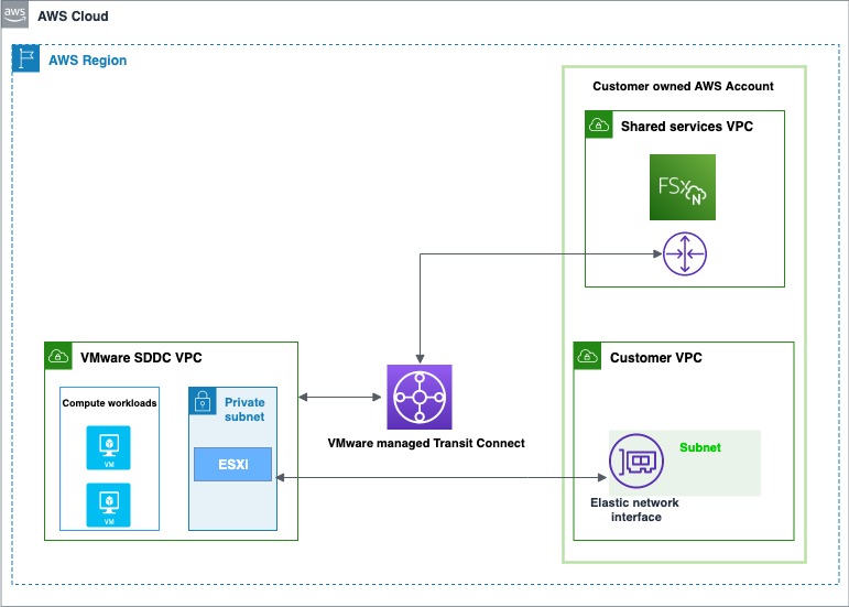
An Overview of VMware Cloud on AWS Integration with Amazon FSx for NetApp ONTAP There are two account connectivity options for enabling storage provisioned by FSx for NetApp ONTAP to be made available for mounting as a datastore to a VMware Cloud on AWS SDDC. Both options use a dedicated Amazon Virtual Private Cloud (Amazon VPC) for the FSx file system to prevent routing conflicts.
The first option is to create a new Amazon VPC under the same connected AWS account and have it connected with the VMware-owned Shadow VPC using VMware Transit Connect. The diagram below shows the architecture of this option:
The first option is to enable storage under the same AWS connected account
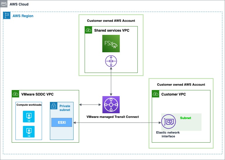
The second option is to create a new AWS account, which by default comes with an Amazon VPC for the Region. Similar to the first option, VMware Transit Connect is used to attach this new VPC with the VMware-owned Shadow VPC. Here is a diagram showing the architecture of this option:
The second option is to enable storage by creating a new AWS account
Getting Started with VMware Cloud on AWS Integration with Amazon FSx for NetApp ONTAP The first step is to create an FSx for NetApp ONTAP file system in your AWS account. The steps that you will follow to do this are the same, whether you’re using the first or second path to provision and mount your NFS datastore.
On the dashboard, choose Create file system to start the file system creation wizard.
On the Select file system type page, select Amazon FSx for NetApp ONTAP, and then click Next which takes you to the Create ONTAP file system page. Here select the Standard create method.
The following video shows a complete guide on how to create an FSx for NetApp ONTAP:
After the file system is created, locate the NFS IP address under the Storage virtual machines tab. The NFS IP address is the floating IP that is used to manage access between file system nodes, and it is required for configuring VMware Transit Connect.
Location of the NFS IP address under the Storage virtual machines tab – AWS console
Location of the NFS IP address under the Storage virtual machines tab – AWS console
You are done with creating the FSx for NetApp ONTAP file system, and now you need to create an SDDC group and configure VMware Transit Connect. In order to do this, you need to navigate between the VMware Cloud Console and the AWS console.
Sign in to the VMware Cloud Console, then go to the SDDC page. Here locate the Actions button and select Create SDDC Group. Once you’ve done this, provide the required data for Name (in the following example I used “FSx SDDC Group” for the name) and Description. For Membership, only include the SDDC in question.
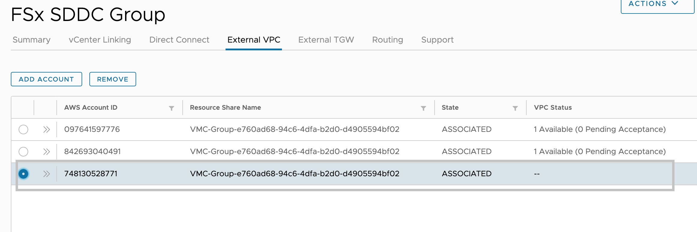
After the SDDC Group is created, it shows up in your list of SDDC Groups. Select the SDDC Group, and then go to the External VPC tab.
External VPC tab Add Account – VMC Console
Once you are in the External VPC tab, click the ADD ACCOUNT button, then provide the AWS account that was used to provision the FSx file system, and then click Add.
Now it’s time for you to go back to the AWS console and sign in to the same AWS account where you created your Amazon FSx file system. Here navigate to the Resource Access Manager service page and click the Accept resource share button.
Resource Access Manager service page to access the Accept resource share button – AWS console
Return to the VMC Console. By now, the External VPC is in an ASSOCIATED state. This can take several minutes to update.
External VPC tab – VMC Console
Next, you need to attach a Transit Gateway to the VPC. For this, navigate back to the AWS console. A step-by-step guide can be found in the AWS Transit Gateway documentation.
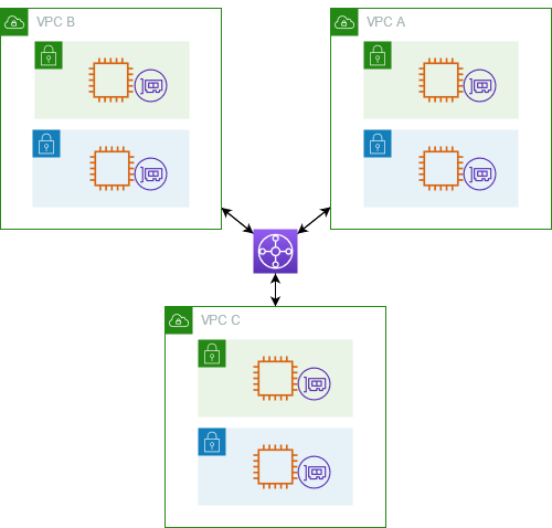
The following is an example that represents a typical architecture of a VPC attached to a Transit Gateway:
A typical architecture of a VPC attached to a Transit Gateway
You are almost at the end of the process. You now need to accept the transit gateway attachment and for this you will navigate back to the VMware Cloud Console.
Accept the Transit Gateway attachment as follows:
Navigating back to the SDDC Group, External VPC tab, select the AWS account ID used for creating your FSx NetApp ONTAP, and click Accept. This process may take a few minutes.
Next, you need to add the routes so that the SDDC can see the FSx file system. This is done on the same External VPC tab, where you will find a table with the VPC. In that table, there is a button called Add Routes. In the Add Route section, add two routes:
The CIDR of the VPC where the FSx file system was deployed.
The floating IP address of the file system.
Click Done to complete the route task.
In the AWS console, create the route back to the SDDC by locating VPC on the VPC service page and navigating to the Route Table as seen below.
VPC service page Route Table navigation – AWS console
Ensure that you have the correct inbound rules for the SDDC Group CIDR by locating Security Groups under VPC and finding the Security Group that is being used (it should be the default one) to allow the inbound rules for SDDC Group CIDR.
Security Groups under VPC that are being used to allow the inbound rules for SDDC Group CIDR
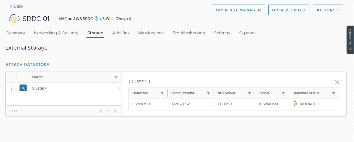
Lastly, mount the NFS Datastore in the VMware Cloud Console as follows:
Locate your SDDC.
After selecting the SDDC, Navigate to the Storage Tab.
Click Attach Datastore to mount the NFS volume(s).
The next step is to select which hosts in the SDDC to mount the datastore to and click Mount to complete the task.
Attach A New Datastore
Available Today Amazon FSx for NetApp ONTAP is available today for VMware Cloud on AWS customers in US East (Ohio), US East (N. Virginia), US West (Oregon), Asia Pacific (Mumbai), Asia Pacific (Seoul), Asia Pacific (Singapore), Asia Pacific (Sydney), Asia Pacific (Tokyo), Canada (Central), Europe (Frankfurt), Europe (Ireland), Europe (London), Europe (Milan), Europe (Paris), Europe (Stockholm), South America (São Paulo), AWS GovCloud (US-East), and AWS GovCloud (US-West).
Cloud workflows are rapidly becoming a driver of every modern media team’s day-to-day creative output. Whether it’s enabling remote shoots, distributed teams, or leveraging budgets more effectively, the cloud can deliver a ton of value to any team. But workflows, by their nature, are complex—and plenty of legacy cloud solutions only add to that complexity with tangled pricing models and limits to egress and collaboration.
ELEMENTS has been simplifying media workflows for more than a decade. Cloud storage has always been part of the ELEMENTS DNA, but they’ll be presenting revolutionary platform updates for cloud workflows in 2023 and beyond at IBC 2022. Part of this new focus on cloud solutions is their addition of an easy, transparent cloud storage option to their platform in Backblaze B2 Cloud Storage. Nimble post-production teams are always on the lookout for more straightforward and easy-to-understand cloud plans with transparent costs—this is a market that Backblaze serves more effectively than the other legacy providers accessible through the platform.
Learn More About This Solution Live in Amsterdam
If you’re attending the 2022 IBC Conference in Amsterdam, join us at stand 7.B06 to learn about integrating B2 Cloud Storage into your workflow. You can schedule a meeting here.
The Backblaze + ELEMENTS Integration
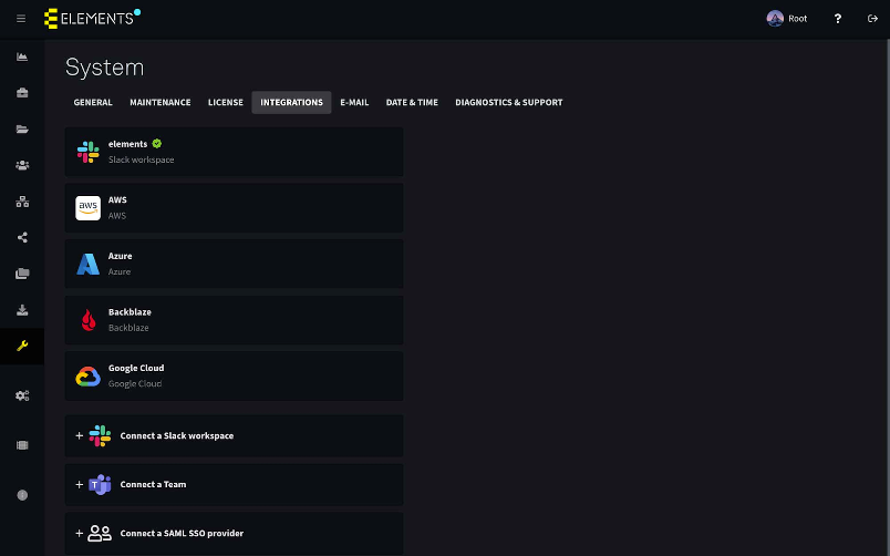
The ELEMENTS platform makes it simple to upload and download files straight from on-premises storage while also offering smart and fully customisable archiving workflows, cloud-based media asset management (MAM), and a number of other tools and features that remove the borders between cloud and on-premises storage. Once connected, ELEMENTS enables users to search, edit, or automate changes to media assets. This extends to team collaboration and setting rights to folders and data across the connected networks. ELEMENTS has provided an intuitive interface making this an easy-to-use solution that is designed for the M&E industry.
Connecting your Backblaze account with ELEMENTS is easy. Simply navigate to the System > Integrations menu and enter your Backblaze login credentials. After this, Backblaze B2 Buckets of the connected account can be mounted as a volume on ELEMENTS.
If you’d like to run a proof of concept with Backblaze, the first 10 GB is free and setting up a Backblaze account only takes a few clicks. Or you can contact sales for more information.
If you’re already a Backblaze B2 customer and would like to check out the ELEMENTS platform, contact ELEMENTS directly here.
Simplifying Your Workflow AND Your Budget
Backblaze focuses on end-to-end ease, including how it works in your budget. Businesses can select a pay-as-you go option or work with a reseller to access capacity plans.
B2 Cloud Storage – This is a general cloud plan for applications, backups and almost all of your business needs. The pricing is simple: $5 per TB per month + $0.01 per GB download fee. As with all plans, the files are located on one storage tier and can always be easily accessed.
B2 Reserve – This is the sweet spot for most media use cases. B2 Reserve is a cloud package starting from 20TB per month. This plan comes at a slightly higher cost than the standard B2 Cloud Storage plan but is free from egress fees up to the amount of storage purchased per month. B2 Reserve will quickly work in your favor if you plan on accessing your files regularly. NOTE: B2 Reserve is only available through resellers.
Top Benefits for Teams Using Backblaze and ELEMENTS Together
The ELEMENTS platform offers a set of robust tools that unlock time and budgets for creative teams to do more. We’ll underline how these different features can work with Backblaze B2.
Automation Engine
The ELEMENTS Automation Engine allows users to create workflows with any number of steps. This tool has a growing list of templates, two of which are Archive and Restore automations. These can be used to archive footage to Backblaze and delete it from the on-premises storage while keeping a lightweight preview proxy. If you need the original footage after previewing the proxy, triggering the Restore automation is all you need to do. The hi-res footage will automatically be downloaded from the Backblaze B2 bucket and placed onto the original location.
A huge benefit of using cloud storage through the ELEMENTS platform is that the individual users do not need to have cloud accounts or direct cloud access. Users will only be able to use the cloud features through the preset automation jobs and according to their permissions.
Media Library
Cloud technologies open up a number of new possibilities within the Media Library, our powerful, browser-based media asset management (MAM) platform.
For example, if your post-production facility has a locally-deployed media library which is running on your ELEMENTS storage and is connected to your Backblaze account, users can playback all of your footage at any time, no matter where it is stored—on-premises, in the cloud, or even in your LTO archive.
The Media Library adds a layer of functionality to the cloud and allows you to easily build a true cloud archive—one that can be accessed from anywhere, in which footage can easily be previewed and just as easily restored with a click of a button.
File Manager
The File Manager is a functionality of the ELEMENTS Web UI that allows you to browse and manage content on your storage on-premises and, very soon, in the cloud. It provides you with a clear overview of all your files, no matter how many file systems and cloud buckets you have. File Managers’ support for cloud storage means users will be able to manage all of their files in one place, without having to navigate through a host of different cloud providers’ interfaces.
ELEMENTS Client
The ELEMENTS Client is an intuitive connection manager that allows admins to decide who gets to mount what—providing a secure gatekeeper to your footage.
The latest function, coming soon to the ELEMENTS Client, will allow users to mount cloud workspaces. This means that users will be able to access the contents of the Backblaze B2 Bucket as if it were a local drive. With optional access logging, users will have the ability to access the cloud-stored content while admins can maintain a high level of security.
Bringing Independent Cloud Storage to the ELEMENTS Platform
Offering B2 Cloud Storage as a native option within the ELEMENTS platform brings a whole new type of cloud offering to Elements’ users. We’re eager to see how creatives use an easier, more affordable, independent option in their workflows.
Learn More About this Solution Live in Amsterdam
If you’re attending the 2022 IBC Conference in Amsterdam, join us at stand 7.B06 to learn about integrating B2 Cloud Storage into your workflow. You can schedule a meeting here.
This week, we are exploring Git’s internals with the following concept in mind:
Git is the distributed database at the core of your engineering system.
Git’s role as a version control system has multiple purposes. One is to help your team make collaborative changes to a common repository. Another purpose is to allow individuals to search and investigate the history of the repository. These history investigations form an interesting query type when thinking of Git as a database.
Not only are history queries an interesting query type, but Git commit history presents interesting data shapes that inform how Git’s algorithms satisfy those queries.
Let’s dig into some common history queries now.
Git history queries
History queries can take several forms. For this post, we are focused only on history queries based entirely on the commits themselves. In part III we will explore file history queries.
Recent commits
Users most frequently interact with commit history using git log to see the latest changes in the current branch. git log shows the commit history which relies on starting at some known commits and then visiting their parent commits and continuing to “walk” parent relationships until all interesting commits are shown to the user. This command can be modified to compare the commits in different branches or display commits in a graphical visualization.
We sometimes also need to get extra information about our commit history, such as asking “which tags contain this commit?” The git tag --contains command is one way to answer that question.
The similar git branch --contains command will report all branches that can reach a given commit. These queries can be extremely valuable. For example, they can help identify which versions of a product have a given bugfix.
Merge base queries
When creating a merge commit, Git uses a three-way merge algorithm to automatically resolve the differences between the two independent commits being merged. As the name implies, a third commit is required: a merge base.
A merge base between two commits is a commit that is in the history of both commits. Technically, any commit in their common history is sufficient, but the three-way merge algorithm works better if the difference between the merge base and each side of the merge is as small as possible.
Git tries to select a single merge base that is not reachable from any other potential merge base. While this choice is usually unique, certain commit histories can permit multiple “best” merge bases, in which case Git prints all of them.
The git merge-base command takes two commits and outputs the object ID of the merge base commit that satisfies all of the properties described earlier.
One thing that can help to visualize merge commits is to explore the boundary between two commit histories. When considering the commit range B..A, a commit C is on the boundary if it is reachable from both A and B and there is at least one commit that is reachable from A and not reachable from B and has C as its parent. In this way, the boundary commits are the commits in the common history that are parents of something in the symmetric difference. There are a number of commits on the boundary of these two example commits, but one of them can reach all of the others providing the unique choice in merge base.
$ git log --graph --oneline --boundary 3d8e3dc4fc..d02cc45c7a
* d02cc45c7a2c Merge branch 'mt/pkt-line-comment-tweak'
|\
| * ce5f07983d18 pkt-line.h: move comment closer to the associated code
* | acdb1e1053c5 Merge branch 'mt/checkout-count-fix'
|\ \
| * | 611c7785e8e2 checkout: fix two bugs on the final count of updated entries
| * | 11d14dee4379 checkout: show bug about failed entries being included in final report
| * | ed602c3f448c checkout: document bug where delayed checkout counts entries twice
* | | f0f9a033ed3c Merge branch 'cl/rerere-train-with-no-sign'
|\ \ \
| * | | cc391fc88663 contrib/rerere-train: avoid useless gpg sign in training
| o | | bbea4dcf42b2 Git 2.37.1
| / /
o / / 3d8e3dc4fc22 Merge branch 'ds/rebase-update-ref' <--- Merge Base
/ /
o / e4a4b31577c7 Git 2.37
/
o 359da658ae32 Git 2.35.4
These simple examples are only a start to the kind of information Git uses from a repository’s commit history. We will discuss some of the important ways the structure of commits can be used to accelerate these queries.
The object ID for the tree representing the root of the worktree at this point in time.
The object IDs for any number of parent commits representing the previous points in time leading to this commit. We use different names for commits based on their parent count:
Zero parents: these commits are the starting point for the history and are called root commits.
One parent: these are typical commits that modify the repository with respect to the single parent. These commits are frequently referred to as patches, since their differences can be communicated in patch format using git format-patch.
Two parents: these commits are called merges because they combine two independent commits into a common history.
Three or more parents: these commits are called _octopus merges_since they combine an arbitrary number of independent commits.
Time information for the author time and committer time, which can be different.
A commit message, which represents additional metadata. This information is mostly intended for human consumption, so you should write it carefully. Some carefully-formatted trailer lines in the message can be useful for automation. One such trailer is the Co-authored-by: trailer which allows having multiple authors of a single commit.
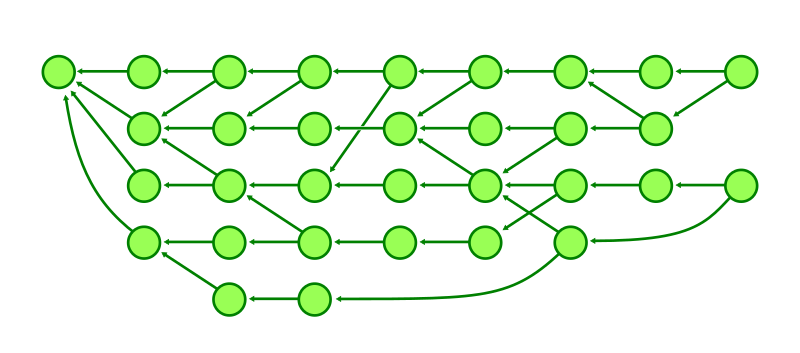
The commit graph is the directed graph whose vertices are the commits in the repository and where a commit has a directed edge to each of its parents. With this representation in mind, we can visualize the commit history as dots and arrows.
Graph databases need not apply
There are a number of graph databases that store general-purpose graph relationships. While it would be possible to store commits, trees, and blobs in such a database, those databases are instead designed for queries of limited-depth. They expect to walk only a few relationships, and maybe there are many relationships from a single node.
When considering general-purpose graph databases, think about social networks. Think about the concept of six degrees of separation and how almost every node is reachable within a short distance. In these graphs, the number of relationships at a given node can vary wildly. Further, the relationships are mainly unordered.
Git is not like that. It is rare to refer to a commit directly by its object ID. Instead Git commands focus on the current set of references. The references are much smaller in number than the total number of commits, and we might need to walk thousands of commit-parent edges before satisfying even the simplest queries.
Git also cares about the order of the parent relationships. When a merge commit is created, the parents are ordered. The first parent has a special role here. The convention is that the first parent is the previous value of the branch being updated by the merge operation. If you use pull requests to update a branch, then you can use git log --first-parent to show the list of merge commits created by that pull request.
$ git log --oneline --first-parent
2d79a03 Merge pull request #797 from ldennington/ssl-cert-updates
e209b3d Merge pull request #790 from cornejom/gitlab-support-docs
b83bf02 Merge pull request #788 from ldennington/arm-fix
cf5a693 (tag: v2.0.785) Merge pull request #778 from GyroJoe/main
dd4fe47 Merge pull request #764 from timsu92/patch-1
428b40a Merge pull request #759 from GitCredentialManager/readme-update
0d6f1c8 (tag: v2.0.779) Merge pull request #754 from mjcheetham/bb-newui
a9d78c1 Merge pull request #756 from mjcheetham/win-manifest
Git’s query pattern is so different from general-purpose graph databases that we need to use specialized storage and algorithms suited to its use case.
Git’s commit-graph file
All of Git’s functionality can be done by loading each commit’s contents out of the object store, parsing its header to discover its parents, and then repeating that process for each commit we need to examine. This is fast enough for small repositories, but as the repository increases in size the overhead of parsing these plain-text files to get the graph relationships becomes too expensive. Even the fact that we need a binary search to locate the object within the packfile begins to add up.
Git’s solution is the commit-graph file. You can create one in your own repository using git commit-graph write --reachable, but likely you already get one through git gc --auto or through background maintenance.
The file acts as a query index by storing a structured version of the commit graph data, such as the parent relationships as well as the commit date and root tree information. This information is sufficient to satisfy the most expensive parts of most history queries. This avoids the expensive lookup and parsing of the commit messages from the object store except when a commit needs to be output to the user.
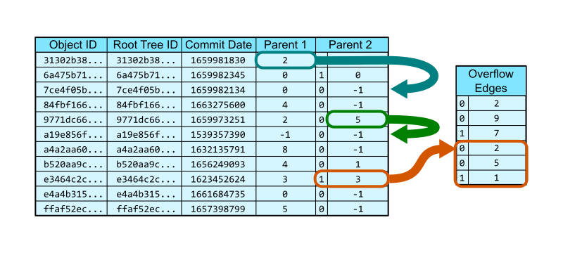
We can think about the commit-graph as a pair of database tables. The first table stores each commit with its object ID, root tree, date, and first two parents as the columns. A special value, -1, is used to indicate that there is no parent in that position, which is important for root commits and patches.
The vast majority of commits have at most two parents, so these two columns are sufficient. However, Git allows an arbitrary number of parents, forming octopus merges. If a commit has three or more parents, then the second parent column has a special bit indicating that it stores a row position in a second table of overflow edges. The remaining parents form a list starting at that row of the overflow edges table, each position stores the integer position of a parent. The list terminates with a parent listed along with a special bit.
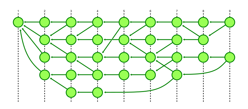
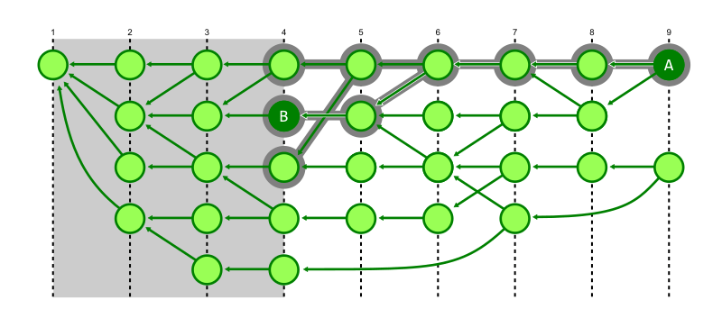
In the figure below, the commit at row 0 has a single parent that exists at row 2. The commit at row 4 is a merge whose second parent is at row 5. The commit at row 8 is an octopus merge with first parent at row 3 and the remaining parents come from the parents table: 2, 5, and 1.
One important thing about the commit-graph file is that it is closed under reachability. That means that if a commit is in the file, then so is its parent. This means that a commit’s parents can be stored as row numbers instead of as full object IDs. This provides a constant-time lookup when traversing between a commit and its parent. It also compresses the commit-graph file since it only needs four bytes per parent.
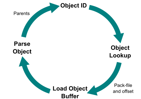
The structure of the commit-graph file speeds up commit history walks significantly, without any changes to the commit walk algorithms themselves. This is mainly due to the time it takes to visit a commit. Without the commit-graph file, we follow this pattern:
Start with an Object ID.
Do a lookup in the object store to see where that object is stored.
Load the object content from the loose object or pack, decompressing the data from disk.
Parse that object file looking for the parent object IDs.
This loop is visualized below.
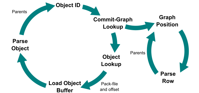
When a commit-graph file exists, we have a way to eject out of this loop and into a much tighter loop. We add an extra step before doing a generic object lookup in the object store: use a binary search to find that object ID in the commit-graph file. This operation is logarithmic in the number of commits, not in the total number of objects in the repository. If the commit-graph does not have that commit, then continue in the old loop. Check the commit-graph each time so we can eventually find a commit and its position in the commit-graph file.
Once we have a commit in the commit-graph file, we can navigate immediately to the row that stores that commit’s information, then load the parent commits by their position. This means that we can lookup the parents in constant time without doing any binary search! This loop is visualized below.
This reduced data footprint makes it clear that we can speed up certain queries on the basis of parsing speed alone. The git rev-list command is great for showing this because it prints the object IDs of the commits and not the commit messages. Thus, we can test how long it takes to walk the full commit graph with and without the commit-graph file.
The Linux kernel repository is an excellent candidate for testing these queries, since it is publicly available and has over a million commits. You can replicate these tests by writing a commit-graph file and toggling the core.commitGraph config setting.
Command
Without commit-graph
With commit-graph
git rev-list v5.19
6.94s
0.98s
git rev-list v5.0..v5.19
2.51s
0.30s
git merge-base v5.0 v5.19
2.59s
0.24s
Avoiding the expensive commit parsing results in a nice constant factor speedup (about 6x in these examples), but we need something more to get even better performance out of certain queries.
Reachability indexes
One of the most important questions we ask about commits is “can commit A reach commit B?” If we can answer that question quickly, then commands such as git tag --contains and git branch --contains become very fast.
Providing a positive answer can be very difficult, and most times we actually want to traverse the full path from A to B, so there is not too much value in that answer. However, we can learn a lot from the opposite answer when we can be sure that A cannot reach B.
The commit-graph file provides a location for adding new information to our commits that do not exist in the commit object format by default. The new information that we store is called a generation number. There are multiple ways to compute a generation number, but the most important property we need to guarantee is the following:
If the generation number of a commit A is less than the generation number of a commit B, then A cannot reach B.
In this way, generation numbers form a negative reachability index in that they can help us determine that some commits definitely cannot reach some other set of commits.
The simplest generation number is called topological level and it is defined this way:
If a commit has no parents, then its topological level is 1.
Otherwise, the topological level of a commit is one more than the maximum of the topological level of its parents.
Our earlier commit graph figure was already organized by topological level, but here it is shown with those levels marked by dashed lines.
The topological level satisfies the property of a generation number because every commit has topological level strictly larger than its parents, which implies that everything that commit can reach has strictly smaller topological level. Conversely, if something has larger topological level, then it is not reachable from that commit.
You may have noticed that I did not mention what is implied when two commits have the same generation number. While we could surmise that equal topological level implies that neither commit can reach the other, it is helpful to leave equality as an unknown state. This is because commits that are in the repository but have not yet been added to the commit-graph file do not have a precomputed generation number. Internally, Git treats these commits as having generation number infinity which is larger than all of the precomputed generation numbers in the commit-graph. However, Git can do nothing when two commits with generation number infinity are compared. Instead of special-casing these commits, Git does not assume anything about equal generation number.
Stopping walks short with generation numbers
Let’s explore how we can use generation numbers to speed up commit history queries. The first category to explore are reachability queries, such as:
git tag --contains <b> returns the list of tags that can reach the commit <b>.
git merge-base --is-ancestor <b> <a> returns an exit code of 0 if and only if <b> is an ancestor of <a> (<b> is reachable from <a>)
Both of these queries seek to find paths to a given point <b>. The natural algorithm is to start walking and report success if we ever discover the commit <b>. However, this might lead to walking every single commit before determining that we cannot in fact reach <b>. Before generation numbers, the best approach was to use a breadth-first search using commit date as a heuristic for walking the most recent commits first. This minimized the number of commits to walk in the case that we did eventually find <b>, but does not help at all if we cannot find <b>.
With generation numbers, we can gain two new enhancements to this search.
The first enhancement is that we can stop exploring a commit if its generation number is below the generation number of our target commit. Those commits of smaller generation could never contribute to a path to the target, so avoid walking them. This is particularly helpful if the target commit is very recent, since that cuts out a huge amount of commits from the search space.
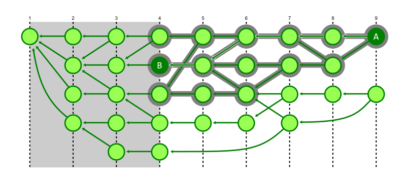
In the figure below, we discover that commit A can reach commit B, but we explored every reachable commit with higher generation. We know that we do not need to explore below generation number 4.
The second enhancement is that we can switch from breadth-first search to a depth-first search. This heuristic exploits some structure about typical repositories. The first parent of a commit is typically special, representing the previous value of the branch before the merge. The later parents are typically small topic branches merging a few new commits into the trunk of the repository. By walking the first parent history, we can navigate quickly to the generation number cutoff where the target commit is likely to be. As we backtrack from that cutoff, we are likely to find the merge commit that introduced the target commit sooner than if we had walked all recent commits first.
In the figure below, we demonstrate the same reachability query from commit A to commit B, where Git avoids walking below generation 4, but the depth-first search also prevents visiting a number of commits that were marked as visited in the previous figure.
Note that this depth-first search approach is less efficient if we do not have the first generation number cutoff optimization, because the walk would spend most of its time exploring very old commits.
These two walks together can introduce dramatic improvements to our reachability queries.
Command
Without commit-graph
With commit-graph
git tag --contains v5.19~100
7.34s
0.04s
git merge-base --is-ancestor v5.0 v5.19
2.64s
0.02s
Note that since git tag --contains is checking reachability starting at every tag, it needs to walk the entire commit history even from old tags in order to be sure they cannot reach the target commit. With generation numbers, the cutoff saves Git from even starting a walk from those old tags. The git merge-base --is-ancestor command is faster even without generation numbers because it can terminate early once the target commit is found.
However, with the commit-graph file and generation numbers, both commands benefit from the depth-first search as the target commit is on the first-parent history from the starting points.
If you’re interested to read the code for this depth-first search in the Git codebase, then read the can_all_from_reach_with_flags() method which is a very general form of the walk. Take a look at how it is used by other callers such as repo_is_descendant_of() and notice how the presence of generation numbers determines which algorithm to use.
Topological sorting
Generation numbers can help other queries where it is less obvious that a reachability index would help. Specifically, git log --graph displays all reachable commits, but uses a special ordering to help the graphical visualization.
git log --graph uses a sorting algorithm called topological sort to present the commits in a pleasing order. This ordering has one hard requirement and one soft requirement.
The hard requirement is that every commit appears before its parents. This is not guaranteed by default in git log, since the default sort uses commit dates as a heuristic during the walk. Commit dates could be skewed and a commit could appear after one of its parents because of date skew.
The soft requirement is that commits are grouped together in an interesting way. When git log --graph shows a merge commit, it shows the commits “introduced” by the merge before showing the first parent. This means that the second parent is shown first followed by all of the commits it can reach that the first parent cannot reach. Typically, this will look like the commits from the topic branch that were merged in that pull request. We can see how this works with the following example from the git/git repository.
Notice that the first example with only --graph brought the commits introduced by the merge to the top of the order. Adding --date-order changes this ordering goal to instead present commits by their commit date, hiding those introduced commits below a long list of merge commits.
The basic algorithm for topological sorting is Kahn’s algorithm which follows two big steps:
Walk all reachable commits, counting the number of times a commit appears as a parent of another commit. Call these numbers the in-degree of the commit, referencing the number of incoming edges.
Walk the reachable commits, but only visit a commit if its in-degree value is zero. When visiting a commit, decrement the in-degree value of each parent.
This algorithm works because at least one of our starting points will have in-degree zero, and then decrementing the in-degree value is similar to deleting the commit from the graph, always having at least one commit with in-degree zero.
But there’s a huge problem with this algorithm! It requires walking all reachable commits before writing even one commit for the user to see. It would be much better if our algorithm would be fast to show the first page of information, so the computation could continue while the user has something to look at.
Typically, Git will show the results in a pager such as less, but we can emulate that experience using a commit count limit with the -n 100 argument. Trying this in the Linux kernel takes over seven seconds!
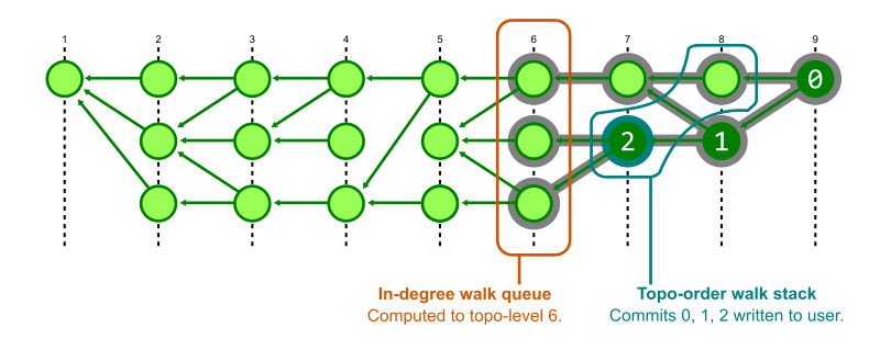
With generation numbers, we can perform an in-line form of Kahn’s algorithm to quickly show the first page of results. The trick is to perform both steps of the algorithm at the same time.
To perform two walks at the same time, Git creates structures that store the state of each walk. The structures are initialized with the starting commits. The in-degree walk uses a priority queue ordered by generation number and that walk starts by computing in-degrees until the maximum generation in that priority queue is below the minimum generation number of the starting positions. The output walk uses a stack, which gives us the nice grouping of commits, but commits are not added unless their in-degree value is zero.
To guarantee that the output walk can add a commit to the stack, it first checks with the status of the in-degree walk to see that the maximum generation in its queue is below the generation number of that commit. In this way, Git alternates between the two walks. It computes just enough of the in-degrees to know that certain commits have an in-degree of zero, then pauses that walk to output some commits to the user.
This has a significant performance improvement for our topological sorting commands.
Command
Without commit-graph
With commit-graph
git rev-list --topo-order -n 100 v5.19
6.88s
0.02s
git log --graph -n 100 v5.19
7.73s
0.03s
git rev-list --topo-order -n 100 v5.18..v5.19
0.39s
0.02s
git log --graph -n 100 v5.18..v5.19
0.43s
0.03s
The top two commands use an unbounded commit range, which is why the old algorithm takes so long: it needs to visit every reachable commit in the in-degree walk before writing anything to output. The new algorithm with generation numbers can explore only the recent commits.
The second two commands use a commit range (v5.18..v5.19) which focuses the search on the commits that are reachable from one commit, but not reachable from another. This actually adds a third stage to the algorithm, where first Git determines which commits are in this range. That algorithm can use a priority queue based on commit date to discover that range without walking the entire commit history, so the old algorithm speeds up for these cases. The in-degree walk still needs to walk that entire range, so it is still slower than the new algorithm as long as that range is big enough.
This idea of a commit range operating on a smaller subgraph than the full commit history actually requires that our interleaved topological sort needs a third walk to determine which commits should be excluded from the output. If you want to learn more about this three-stage algorithm, then read the commit that introduced the walk to Git’s codebase for the full details.
Generation number v2: corrected commit dates
The earlier definition of a generation number was intentionally generic. This is because there are actually multiple possible generation numbers even in the Git codebase!
The definition of topological level essentially uses the smallest possible integer that could be used to satisfy the property of a generation number. The simplicity is nice for understanding, but it has a drawback. It is possible to make the algorithms using generation number worse if you create your commit history in certain ways.
Most of the time, merge commits introduce a short list of recent commits into the commit history. However, some times those merges introduce a commit that’s based on a very old commit. This can happen when fixing a bug in a really old area of code and the developer wants to apply the fix as early as possible so it can merge into old maintenance branches. However, this means that the topological level is much smaller for that commit than for other commits created at similar times.
In this sense, the commit date is a much better heuristic for limiting the commit walk. The only problem is that we can’t trust it as an accurate generation number! Here is where a solution was found: a new generation number based on commit dates. This was implemented as part of a Google Summer of Code project in 2020.
The corrected commit date is defined as follows:
If a commit has no parents, then its corrected commit date is the same as its commit date.
Otherwise, determine the maximum corrected commit date of the commit’s parents. If that maximum is larger than the commit date, then add one to that maximum. Otherwise, use the commit date.
Using corrected commit date leads to a wider variety of values in the generation number of each commit in the commit graph. The figure below is the same graph as in the earlier examples, but the commits have been shifted as they could be using corrected commit dates on the horizontal axis.
This definition flips the generation number around. If possible, use the commit date. If not, use the smallest possible value that satisfies the generation number properties with respect to the corrected commit dates of the commit’s parents.
In performance testing, corrected commit dates solve these performance issues due to recent commits based on old commits. In addition, some Git commands generally have slight improvements over topological levels.
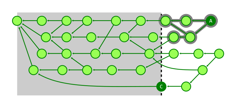
For example, the search from A to C in the figure below shows how many commits must be visited to determine that A cannot reach C when using topological level.
However, switching to using corrected commit dates, the search space becomes much smaller.
We’ve gone very deep into the commit-graph file and reachability algorithms. The on-disk file format is customized to Git’s needs when answering these commit history queries. Thus, it is a type of query index much like one could define in an application database. The rabbit hole goes deeper, though, with yet another level of query index specialized to other queries.
Make sure that you have a commit-graph file accelerating your Git repositories! You can ensure this happens in one of several ways:
Manually run git commit-graph write --reachable.
Enable the fetch.writeCommitGraph config option.
Run git maintenance start and let Git write it in the background.
In the next part of this blog series, we will explore how Git file history queries use the structure of tree objects and the commit graph to limit how many objects need to be parsed. We’ll also talk about a special file history index that is stored in the commit-graph and greatly accelerates file history queries in large repositories.
I’ll also be speaking at Git Merge 2022 covering all five parts of this blog series, so I look forward to seeing you there!
Amazon Redshift Serverless makes it easy to run and scale analytics in seconds without the need to setup and manage data warehouse clusters. With Redshift Serverless, users such as data analysts, developers, business professionals, and data scientists can get insights from data by simply loading and querying data in the data warehouse.
With Redshift Serverless, you can benefit from the following features:
Access and analyze data without the need to set up, tune, and manage Amazon Redshift clusters
Use Amazon Redshift’s SQL capabilities, industry-leading performance, and data lake integration to seamlessly query data across a data warehouse, data lake, and databases
Deliver consistently high performance and simplified operations for even the most demanding and volatile workloads with intelligent and automatic scaling, without under-provisioning or over-provisioning the compute resources
Pay for the compute only when the data warehouse is in use
In this post, we discuss four different use cases of Redshift Serverless:
Easy analytics – A startup company needs to create a new data warehouse and reports for marketing analytics. They have very limited IT resources, and need to get started quickly and easily with minimal infrastructure or administrative overhead.
Self-service analytics – An existing Amazon Redshift customer has a provisioned Amazon Redshift cluster that is right-sized for their current workload. A new team needs quick self-service access to the Amazon Redshift data to create forecasting and predictive models for the business.
Optimize workload performance – An existing Amazon Redshift customer is looking to optimize the performance of their variable reporting workloads during peak time.
Cost-optimizationof sporadic workloads – An existing customer is looking to optimize the cost of their Amazon Redshift producer cluster with sporadic batch ingestion workloads.
Easy analytics
In our first use case, a startup company with limited resources needs to create a new data warehouse and reports for marketing analytics. The customer doesn’t have any IT administrators, and their staff is comprised of data analysts, a data scientist, and business analysts. They want to create new marketing analytics quickly and easily, to determine the ROI and effectiveness of their marketing efforts. Given their limited resources, they want minimal infrastructure and administrative overhead.
In this case, they can use Redshift Serverless to satisfy their needs. They can create a new Redshift Serverless endpoint in a few minutes and load their initial few TBs of marketing dataset into Redshift Serverless quickly. Their data analysts, data scientists, and business analysts can start querying and analyzing the data with ease and derive business insights quickly without worrying about infrastructure, tuning, and administrative tasks.
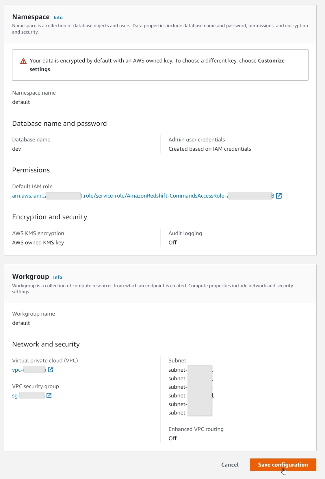
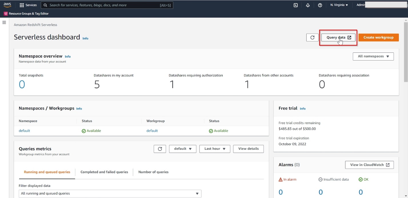
Getting started with Redshift Serverless is easy and quick. On the Get started with Amazon Redshift Serverless page, you can select the Use default settings option, which will create a default namespace and workgroup with the default settings, as shown in the following screenshots.
With just a single click, you can create a new Redshift Serverless endpoint in minutes with data encryption enabled, and a default AWS Identity and Access Management (IAM) role, VPC, and security group attached. You can also use the Customize settings option to override these settings, if desired.
When the Redshift Serverless endpoint is available, choose Query data to launch the Amazon Redshift Query Editor v2.
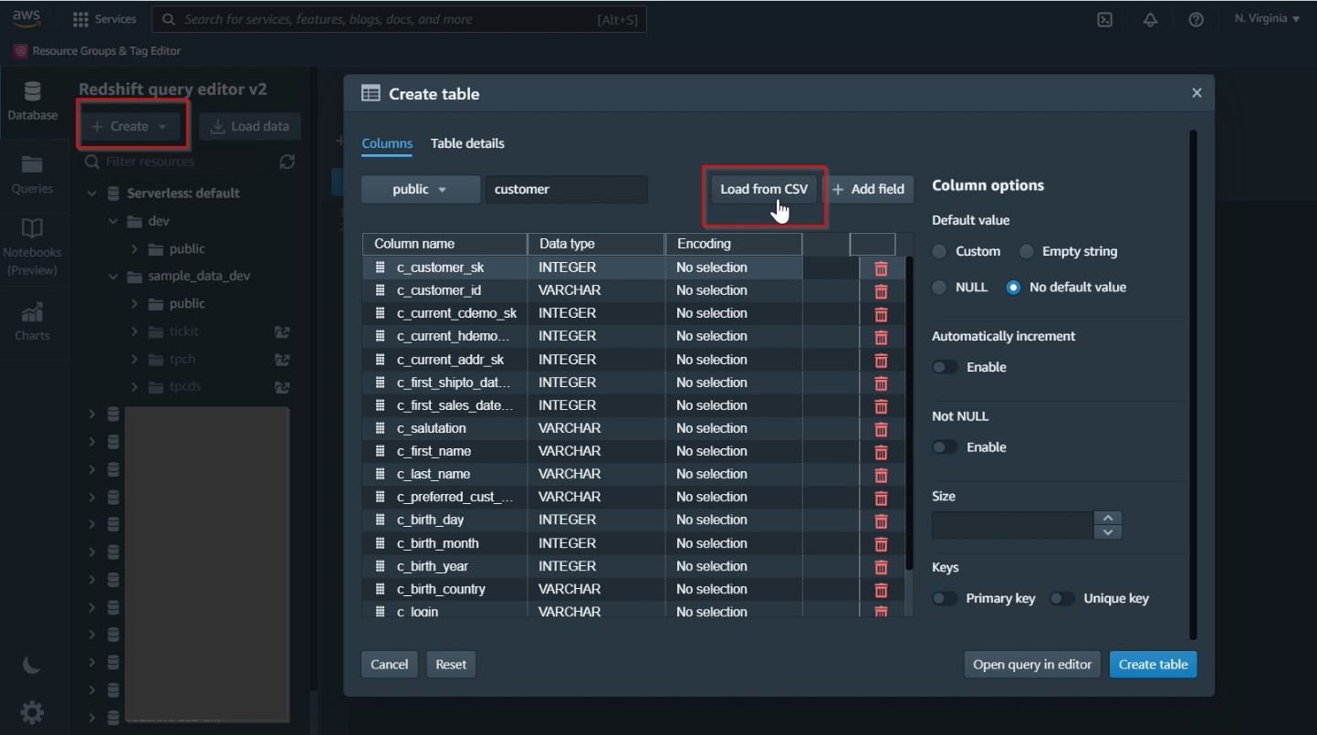
Query Editor v2 makes it easy to create database objects, load data, analyze and visualize data, and share and collaborate with your teams.
The following screenshot illustrates creating new database tables using the UI.
In another use case, a customer is currently using an Amazon Redshift provisioned cluster that is right-sized for their current workloads. A new data science team wants quick access to the Amazon Redshift cluster data for a new workload that will build predictive models for forecasting. The new team members don’t know yet how long they will need access and how complex their queries will be.
Adding the new data science group to the current cluster presented the following challenges:
The additional compute capacity needs of the new team are unknown and hard to estimate
Because the current cluster resources are optimally utilized, they need to ensure workload isolation to support the needs of the new team without impacting existing workloads
A chargeback or cost allocation model is desired for the various teams consuming data
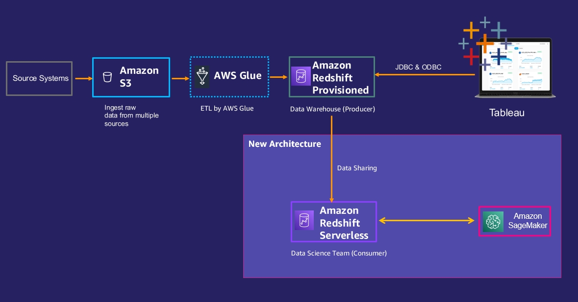
To address these issues, they decide to let the data science team create their own new Redshift Serverless instance and grant them data share access to the data they need from the existing Amazon Redshift provisioned cluster. The following diagram illustrates the new architecture.
The following steps need to be performed to implement this architecture:
The data science team can create a new Redshift Serverless endpoint, as described in the previous use case.
Enable data sharing between the Amazon Redshift provisioned cluster (producer) and the data science Redshift Serverless endpoint (consumer) using these high-level steps:
Create a new data share.
Add a schema to the data share.
Add objects you want to share to the data share.
Grant usage on this data share to the Redshift Serverless consumer namespace, using the Redshift Serverless endpoint’s namespace ID.
Note that the Redshift Serverless endpoint is encrypted by default; the provisioned Redshift producer cluster also needs to be encrypted for data sharing to work between them.
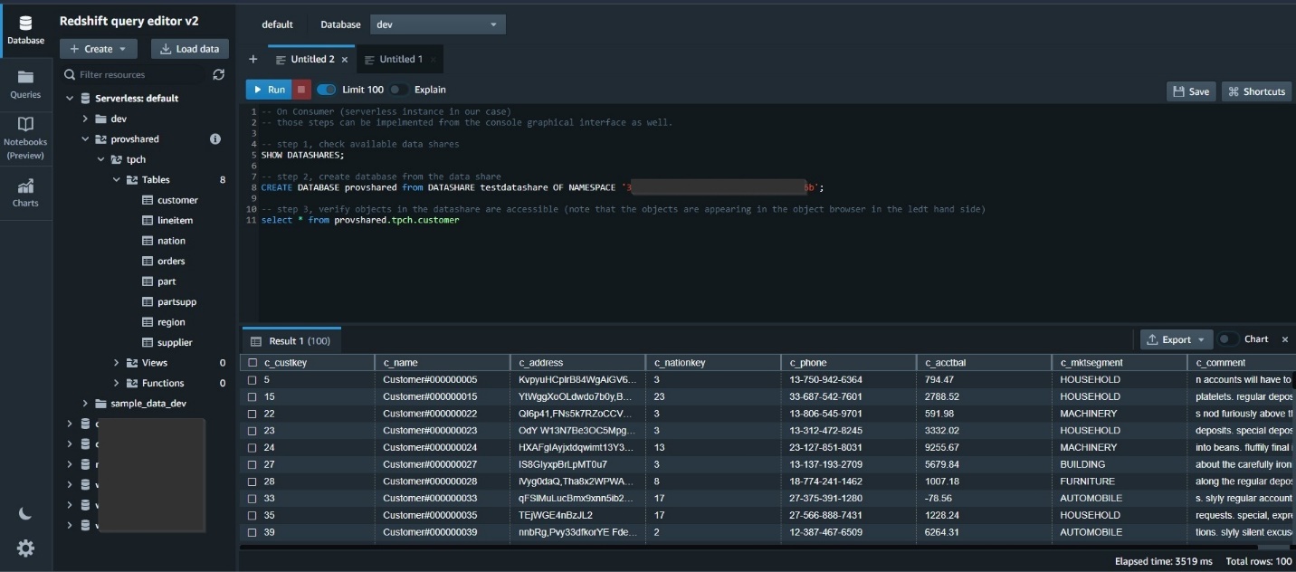
The following screenshot shows sample SQL commands to enable data sharing on the Amazon Redshift provisioned producer cluster.
On the Amazon Redshift Serverless consumer, create a database from the data share and then query the shared objects.
With this architecture, we can resolve the three challenges mentioned earlier:
Redshift Serverless allows the data science team to create a new Amazon Redshift database without worrying about capacity needs, and set up data sharing with the Amazon Redshift provisioned producer cluster within 30 minutes. This tackles the first challenge.
Amazon Redshift data sharing allows you to share live, transactionally consistent data across provisioned and Serverless Redshift databases, and data sharing can even happen when the producer is paused. The new workload is isolated and runs on its own compute resources, without impacting the performance of the Amazon Redshift provisioned producer cluster. This addresses the second challenge.
Redshift Serverless isolates the cost of the new workload to the new team and enables an easy chargeback model. This tackles the third challenge.
Optimized workload performance
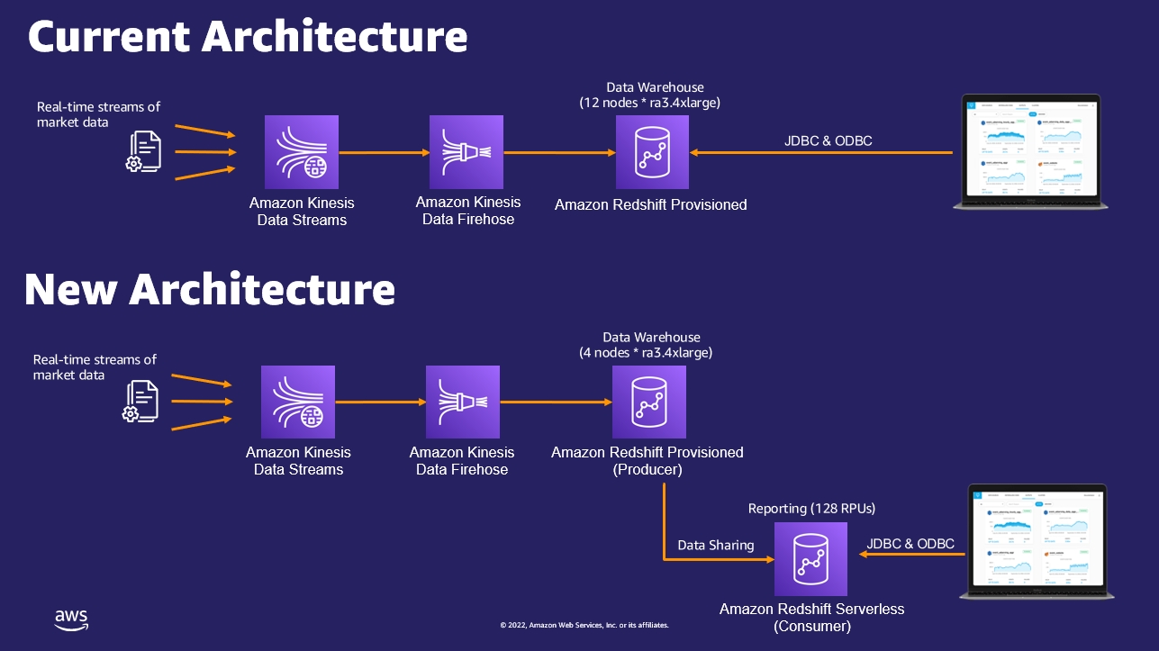
For our third use case, an Amazon Redshift customer using an Amazon Redshift provisioned cluster is looking for performance optimization during peak times for their workload. They need a solution to manage dynamic workloads without over-provisioning or under-provisioning resources and build a scalable architecture.
An analysis of the workload on the cluster shows that the cluster has two different workloads:
The first workload is streaming ingestion, which runs steadily during the day.
The second workload is reporting, which runs on an ad hoc basis during the day with some scheduled jobs during the night. It was noted that the reporting jobs run anywhere between 8–12 hours daily.
The provisioned cluster was sized as 12 nodes of ra3.4xlarge to handle both workloads running in parallel.
To optimize these workloads, the following architecture was proposed and implemented:
Configure an Amazon Redshift provisioned cluster with just 4 nodes of ra3.4xlarge, to handle the streaming ingestion workload only. The following screenshots illustrate how to do this on the Amazon Redshift console, via an elastic resize operation of the existing Amazon Redshift provisioned cluster by reducing number of nodes from 12 to 4:
Create a new Redshift Serverless endpoint to be utilized by the reporting workload with 128 RPU (Redshift Processing Units) in lieu of 8 nodes ra3.4xlarge. For more details about setting up Redshift Serverless, refer to the first use case regarding easy analytics.
Enable data sharing between the Amazon Redshift provisioned cluster as the producer and Redshift Serverless as the consumer using the serverless namespace ID, similar to how it was configured earlier in the self-service analytics use case. For more information about how to configure Amazon Redshift data sharing, refer to Sharing Amazon Redshift data securely across Amazon Redshift clusters for workload isolation.
The following diagram compares the current architecture and the new architecture using Redshift Serverless.
After completing this setup, the customer ran the streaming ingestion workload on the Amazon Redshift provisioned instance (producer) and reporting workloads on Redshift Serverless (consumer) based on the recommended architecture. The following improvements were observed:
The streaming ingestion workload performed the same as it did on the former 12-node Amazon Redshift provisioned cluster.
Reporting users saw a performance improvement of 30% by using Redshift Serverless. It was able to scale compute resources dynamically within seconds, as additional ad hoc users ran reports and queries without impacting the streaming ingestion workload.
This architecture pattern is expandable to add more consumers like data scientists, by setting up another Redshift Serverless instance as a new consumer.
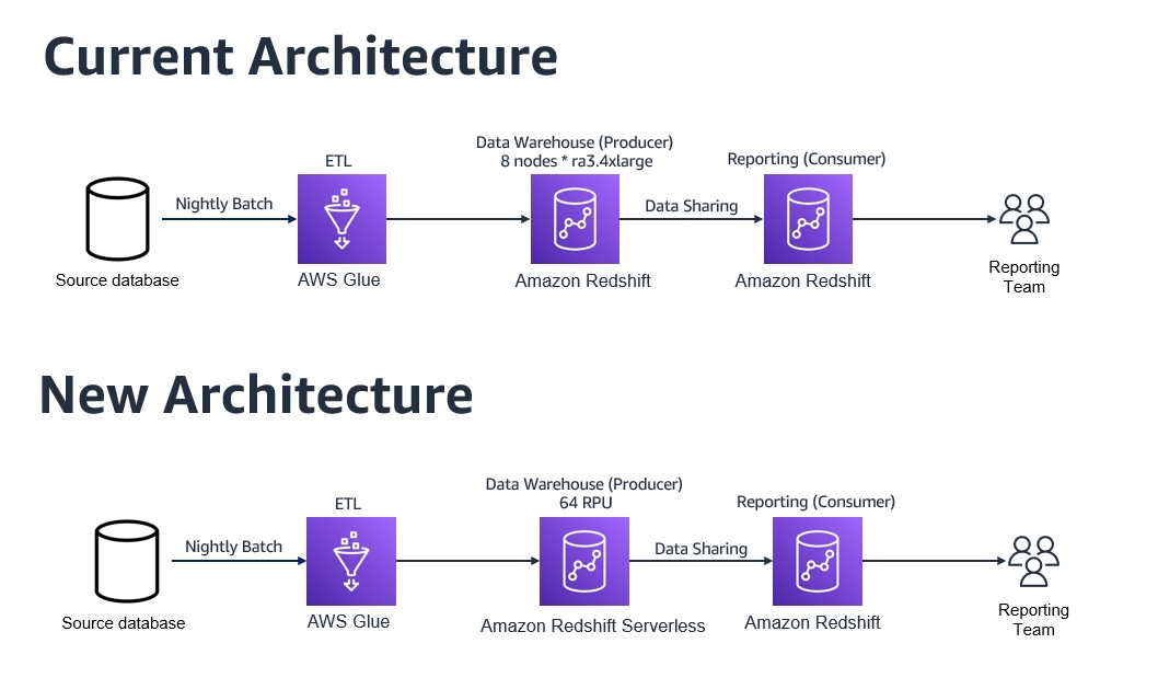
Cost-optimization
In our final use case, a customer is using an Amazon Redshift provisioned cluster as a producer to ingest data from different sources. The data is then shared with other Amazon Redshift provisioned consumer clusters for data science modeling and reporting purposes.
Their current Amazon Redshift provisioned producer cluster has 8 nodes of ra3.4xlarge and is located in the us-east-1 Region. The data delivery from the different data sources is scattered between midnight to 8:00 AM, and the data ingestion jobs take around 3 hours to run in total every day. The customer is currently on the on-demand cost model and has scheduled daily jobs to pause and resume the cluster to minimize costs. The cluster resumes every day at midnight and pauses at 8:00 AM, with a total runtime of 8 hours a day.
The current annual cost of this cluster is 365 days * 8 hours * 8 nodes * $3.26 (node cost per hour) = $76,153.6 per year.
To optimize the cost of this workload, the following architecture was proposed and implemented:
Set up a new Redshift Serverless endpoint with 64 RPU as the base configuration to be utilized by the data ingestion producer team. For more information about setting up Redshift Serverless, refer to the first use case regarding easy analytics.
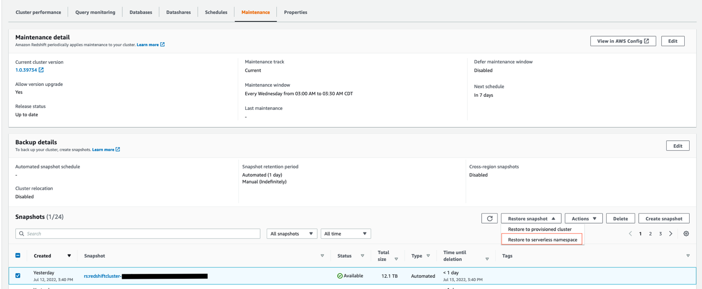
Restore the latest snapshot from the existing Amazon Redshift provisioned producer cluster into Redshift Serverless by choosing the Restore to serverless namespace option, as shown in the following screenshot.
Enable data sharing between Redshift Serverless as the producer and the Amazon Redshift provisioned cluster as the consumer, similar to how it was configured earlier in the self-service analytics use case.
The following diagram compares the current architecture to the new architecture.
By moving to Redshift Serverless, the customer realized the following benefits:
Cost savings – With Redshift Serverless, the customer pays for compute only when the data warehouse is in use. In this scenario, the customer observed a savings of up to 65% on their annual costs by using Redshift Serverless as the producer, while still getting better performance on their workloads. The Redshift Serverless annual cost in this case equals 365 days * 3 hours * 64 RPUs * $0.375 (RPU cost per hour) = $26,280, compared to $76,153.6 for their former provisioned producer cluster. Also, the Redshift Serverless 64 RPU baseline configuration offers the customer more compute resources than their former 8 nodes of ra3.4xlarge cluster, resulting in better performance overall.
Less administration overhead – Because the customer doesn’t need to worry about pausing and resuming their Amazon Redshift cluster any more, the administration of their data warehouse is simplified by moving their producer Amazon Redshift cluster to Redshift Serverless.
Conclusion
In this post, we discussed four different use cases, demonstrating the benefits of Amazon Redshift Serverless—from its easy analytics, ease of use, superior performance, and cost savings that can be realized from the pay-per-use pricing model.
Amazon Redshift provides flexibility and choice in data warehousing. Amazon Redshift Provisioned is a great choice for customers who need a custom provisioning environment with more granular controls; and with Redshift Serverless, you can start new data warehousing workloads in minutes with dynamic auto scaling, no infrastructure management, and a pay-per-use pricing model.
Ahmed Shehata is a Data Warehouse Specialist Solutions Architect with Amazon Web Services, based out of Toronto.
Manish Vazirani is an Analytics Platform Specialist at AWS. He is part of the Data-Driven Everything (D2E) program, where he helps customers become more data-driven.
Rohit Bansal is an Analytics Specialist Solutions Architect at AWS. He has nearly two decades of experience helping customers modernize their data platforms. He is passionate about helping customers build scalable, cost-effective data and analytics solutions in the cloud. In his spare time, he enjoys spending time with his family, travel, and road cycling.
Today we are excited to announce thresholds for our Security Event Alerts: a new and improved way of detecting anomalous spikes of security events on your Internet properties. Previously, our calculations were based on z-score methodology alone, which was able to determine most of the significant spikes. By introducing a threshold, we are able to make alerts more accurate and only notify you when it truly matters. One can think of it as a romance between the two strategies. This is the story of how they met.
Author’s note: as an intern at Cloudflare I got to work on this project from start to finish from investigation all the way to the final product.
Once upon a time
In the beginning, there were Security Event Alerts. Security Event Alerts are notifications that are sent whenever we detect a threat to your Internet property. As the name suggests, they track the number of security events, which are requests to your application that match security rules. For example, you can configure a security rule that blocks access from certain countries. Every time a user from that country tries to access your Internet property, it will log as a security event. While a security event may be harmless and fired as a result of the natural flow of traffic, it is important to alert on instances when a rule is fired more times than usual. Anomalous spikes of too many security events in a short period of time can indicate an attack. To find these anomalies and distinguish between the natural number of security events and that which poses a threat, we need a good strategy.
The lonely life of a z-score
Before a threshold entered the picture, our strategy worked onlyon the basis of a z-score. Z-score is a methodology that looks at the number of standard deviations a certain data point is from the mean. In our current configuration, if a spike crosses the z-score value of 3.5, we send you an alert. This value was decided on after careful analysis of our customers’ data, finding it the most effective in determining a legitimate alert. Any lower and notifications will get noisy for smaller spikes. Any higher and we may miss out on significant events. You can read more about our z-score methodology in this blog post.
The following graphs are an example of how the z-score method works. The first graph shows the number of security events over time, with a recent spike.
To determine whether this spike is significant, we calculate the z-score and check if the value is above 3.5:
As the graph shows, the deviation is above 3.5 and so an alert is triggered.
However, relying on z-score becomes tricky for domains that experience no security events for a long period of time. With many security events at zero, the mean and standard deviation depress to zero as well. When a non-zero value finally appears, it will always be infinite standard deviations away from the mean. As a result, it will always trigger an alert even on spikes that do not pose any threat to your domain, such as the below:
With five security events, you are likely going to ignore this spike, as it is too low to indicate a meaningful threat. However, the z-score in this instance will be infinite:
Since a z-score of infinity is greater than 3.5, an alert will be triggered. This means that customers with few security events would often be overwhelmed by event alerts that are not worth worrying about.
Letting go of zeros
To avoid the mean and standard deviation becoming zero and thus alerting on every non-zero spike, zero values can be ignored in the calculation. In other words, to calculate the mean and standard deviation, only data points that are higher than zero will be considered.
With those conditions, the same spike to five security events will now generate a different z-score:
Great! With the z-score at zero, it will no longer trigger an alert on the harmless spike!
But what about spikes that could be harmful? When calculations ignore zeros, we need enough non-zero data points to accurately determine the mean and standard deviation. If only one non-zero value is present, that data point determines the mean and standard deviation. As such, the mean will always be equal to the spike, z-score will always be zero and an alert will never be triggered:
For a spike of 1000 events, we can tell that there is something wrong and we should trigger an alert. However, because there is only one non-zero data point, the z-score will remain zero:
The z-score does not cross the value 3.5 and an alert will not be triggered.
So what’s better? Including zeros in our calculations can skew the results for domains with too many zero events and alert them every time a spike appears. Not including zeros is mathematically wrong and will never alert on these spikes.
Threshold, the prince charming
Clearly, a z-score is not enough on its own.
Instead, we paired up the z-score with a threshold. The threshold represents the raw number of security events an Internet property can have, below which an alert will not be sent. While z-score checks whether the spike is at least 3.5 standard deviations above the mean, the threshold makes sure it is above a certain static value. If both of these conditions are met, we will send you an alert:
The above spike crosses the threshold of 200 security events. We now have to check that the z-score is above 3.5:
The z-score value crosses 3.5 and an alert will be sent.
A threshold for the number of security events comes as the perfect complement. By itself, the threshold cannot determine whether something is a spike, and would simply alert on any value crossing it. This blog post describes in more detail why thresholds alone do not work. However, when paired with z-score, they are able to share their strengths and cover for each other’s weaknesses. If the z-score falsely detects an insignificant spike, the threshold will stop the alert from triggering. Conversely, if a value does cross the security events threshold, the z-score ensures there is a reasonable variance from the data average before allowing an alert to be sent.
The invaluable value
To foster a successful relationship between the z-score and security events threshold, we needed to determine the most effective threshold value. After careful analysis of our previous attacks on customers, we set the value to 200. This number is high enough to filter out the smaller, noisier spikes, but low enough to expose any threats.
Am I invited to the wedding?
Yes, you are! The z-score and threshold relationship is already enabled for all WAF customers, so all you need to do is sit back and relax. For enterprise customers, the threshold will be applied to each type of alert enabled on your domain.
Happily ever after
The story certainly does not end here. We are constantly iterating on our alerts, so keep an eye out for future updates on the road to make our algorithms even more personalized for your Internet properties!
As a unified SIEM and XDR solution, InsightIDR gives organizations the tools they need to drive an elevated and efficient compliance program.
Cybersecurity standards and compliance are mission-critical for every organization, regardless of size. Apart from the direct losses resulting from a data breach, non-compliant companies could face hefty fees, loss of business, and even jail time under growing regulations. However, managing and maintaining compliance, preparing for audits, and building necessary reports can be a full-time job, which might not be in the budget. For already-lean teams, compliance can also distract from more critical security priorities like monitoring threats, early threat detection, and accelerated response – exposing organizations to greater risk.
An efficient compliance strategy reduces risk, ensures that your team is always audit-ready, and – most importantly – drives focus on more critical security work. With InsightIDR, security practitioners can quickly meet their compliance and regulatory requirements while accelerating their overall detection and response program.
Here are three ways InsightIDR has been built to elevate and simplify your compliance processes.
1. Powerful log management capabilities for full environment visibility and compliance readiness
Complete environment visibility and security log collection are critical for compliance purposes, as well as for providing a foundation of effective monitoring and threat detection. Enterprises need to monitor user activity, behavior, and application access across their entire environment — from the cloud to on-premises services. The adoption of cloud services continues to increase, creating even more potential access points for teams to keep up with.
InsightIDR’s strong log management capabilities provide full visibility into these potential threats, as well as enable robust compliance reporting by:
Centralizing and aggregating all security-relevant events, making them available for use in monitoring, alerting, investigation, ad hoc searching
Providing the ability to search for data quickly, create data models and pivots, save searches and pivots as reports, configure alerts, and create dashboards
Retaining all log data for 13 months for all InsightIDR customers, enabling the correlation of data over time and meeting compliance mandates.
Automatically mapping data to compliance controls, allowing analysts to create comprehensive dashboards and reports with just a few clicks
To take it a step further, InsightIDR’s intuitive user interface streamlines searches while eliminating the need for IT administrators to master a search language. The out-of-the-box correlation searches can be invoked in real time or scheduled to run regularly at a specific time should the need arise for compliance audits and reporting, updated dashboards, and more.
2. Predefined compliance reports and dashboards to keep you organized and consistent
Pre-built compliance content in InsightIDR enables teams to create robust reports without investing countless hours manually building and correlating data to provide information on the organization’s compliance posture. With the pre-built reports and dashboards, you can:
Automatically map data to compliance controls
Save filters and searches, then duplicate them across dashboards
Create, share, and customize reports right from the dashboard
Make reports available in multiple formats like PDF or interactive HTML files
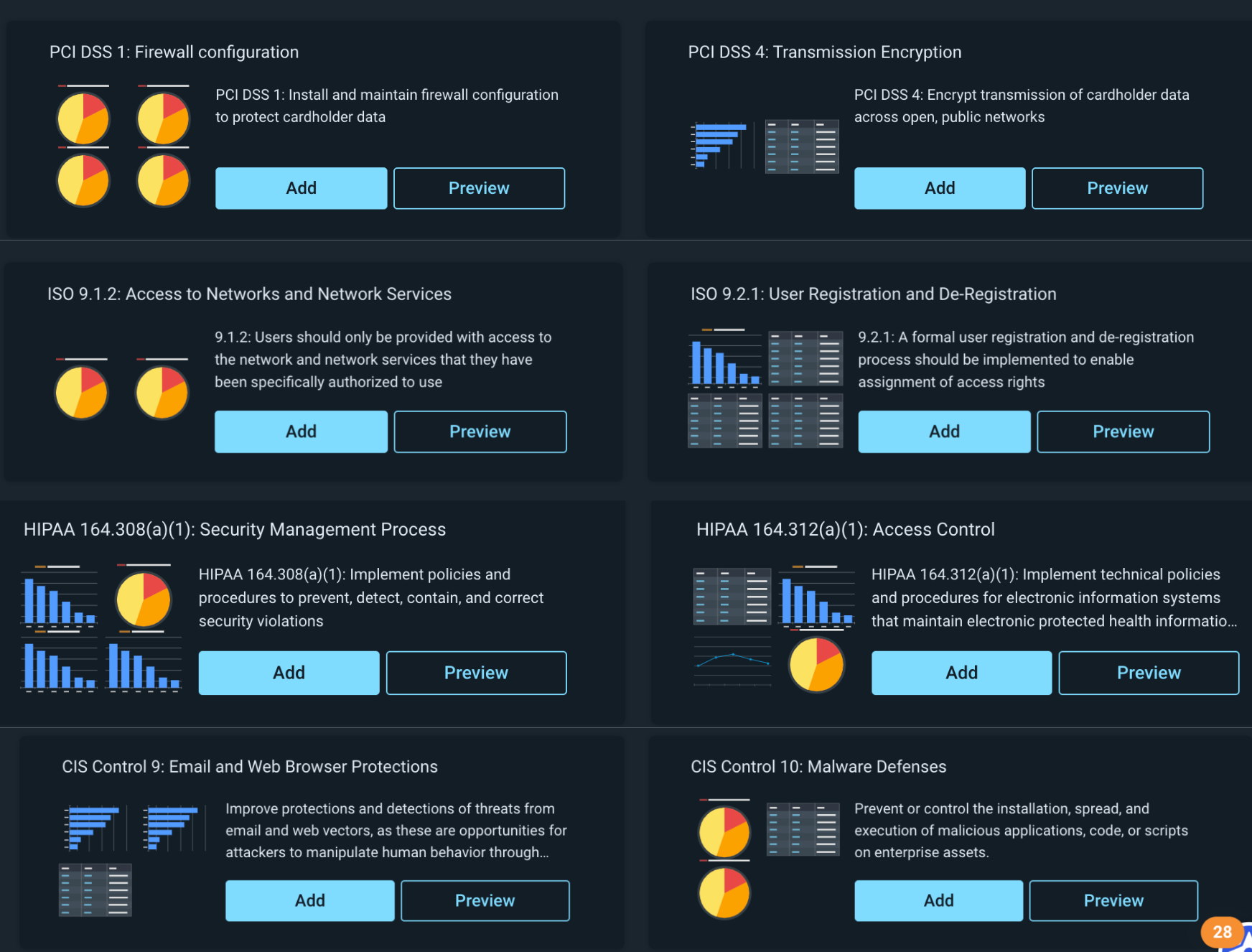
InsightIDR’s library of pre-built dashboards makes it easier than ever to visualize your data within the context of common frameworks. Entire dashboards created by our Rapid7 experts can be set up in just a few clicks. Our dashboards cover a variety of key compliance frameworks like PCI, ISO 27001, HIPAA, and more.
3. Unified and correlated data points to provide meaningful insights
With strong log management capabilities providing a foundation for your security posture, the ability to correlate the resulting data and look for unusual behavior, system anomalies, and other indicators of a security incident is key. This information is used not only for real-time event notification but also for compliance audits and reporting, performance dashboards, historical trend analysis, and post-hoc incident forensics.
Privileged users are often the targets of attacks, and when compromised, they typically do the most damage. That’s why it’s critical to extend monitoring to these users. In fact, because of the risk involved, privileged user monitoring is a common requirement for compliance reporting in many regulated industries.
InsightIDR provides a constantly curated library of detections that span user behavior analytics, endpoints, file integrity monitoring, network traffic analysis, and cloud threat detection and response – supported by our own native endpoint agent, network sensor, and collection software. User authentications, locational data, and asset activity are baselined to identify anomalous privilege escalations, lateral movement, and compromised credentials. Customers can also connect their existing Privileged Access Management tools (like CyberArk Vault or Varonis DatAdvantage) to get a more unified view of privileged user monitoring with a single interface.
Meet compliance standards while accelerating your detection and response
We know compliance is not the only thing a security operations center (SOC) has to worry about. InsightIDR can ensure that your most critical compliance requirements are met quickly and confidently. Once you have an efficient compliance process, the team will be able to focus their time and effort on staying ahead of emergent threats and remediating attacks quickly, reducing risk to the business.
Security updates have been issued by Debian (thunderbird), Fedora (ctk, dcmtk, OpenImageIO, and varnish-modules), Red Hat (systemd), SUSE (libslirp, open-vm-tools, and opera), and Ubuntu (jupyter-notebook, libsdl1.2, and systemd).
The Federal Trade Commission (FTC) has sued Kochava, a large location data provider, for allegedly selling data that the FTC says can track people at reproductive health clinics and places of worship, according to an announcement from the agency.
“Defendant’s violations are in connection with acquiring consumers’ precise geolocation data and selling the data in a format that allows entities to track the consumers’ movements to and from sensitive locations, including, among others, locations associated with medical care, reproductive health, religious worship, mental health temporary shelters, such as shelters for the homeless, domestic violence survivors, or other at risk populations, and addiction recovery,” the lawsuit reads.
Builders create AWS Step Functions workflows to orchestrate multiple services into business-critical applications with minimal code. Customers are looking for best practices and guidelines to build cost-effective workflows with Step Functions.
This blog post explains the difference between Standard and Express Workflows. It shows the cost of running the same workload as Express or Standard Workflows. Then it covers how to migrate from Standard to Express, how to combine workflow types to optimize for cost, and how to modularize and nest one workflow inside another.
Step Functions Express Workflows
Express Workflows orchestrate AWS services at a higher throughput of up to 100,000 state transitions per second. It also provides a lower cost of $1.00 per million invocations versus $25 per million for Standard Workflows.
Express Workflows can run for a maximum duration of 5 minutes and do not support the .waitForTaskToken or .sync integration pattern. Most Step Functions workflows that do not use these integrations patterns and complete within the 5-minute duration limit see both cost and throughput optimizations by converting the workflow type from Standard to Express.
Consider the following example, a naïve implementation of an ecommerce workflow:
When started, it emits a message onto an Amazon SQS queue. An AWS Lambda function processes and approves this asynchronously (not shown). Once processed, the Lambda function persists the state to an Amazon DynamoDB table. The workflow polls the table to check when the action is completed. It then moves on to process the payment, where it repeats the pattern. Finally, the workflow runs a series of update tasks in sequence before completing.
I run this workflow 1,000 times as a Standard workflow. I then convert this to an Express Workflow and run another 1,000 times. I create an Amazon CloudWatch dashboard to display the average execution times. The Express Workflow runs on average 0.5 seconds faster than the Standard Workflow and also shows improvements in cost:
Workflow Execution times
Running the Standard Workflow 1,000 times costs approximately $0.42. This excludes the 4,000 state transitions included in the AWS Free Tier every month, and the additional services that are being used. In contrast to this, running the Express Workflow 1000 times costs $0.01. How is this calculated?
Standard Workflow cost calculation formula:
Standard Workflows are charged based on the number of state transitions required to run a workload. Step Functions count a state transition each time a step of your workflow runs. You are charged for the total number of state transitions across all your state machines, including retries. The cost is $0.025 per 1,000 state transitions.
A happy path through the workflow comprises 17 transitions (including start and finish).
Total cost = (number of transitions per execution x number of executions) x $0.000025 Total cost = (17 X 1000) X 0.000025 = $0.42*
*Excluding the 4,000 state transitions included in the AWS Free Tier every month.
Express Workflow cost calculation formula:
Express Workflows are charged based on the number of requests and its duration. Duration is calculated from the time that your workflow begins running until it completes or otherwise finishes, rounded up to the nearest 100 ms, and the amount of memory used in running your workflow, billed in 64-MB chunks.
Total cost = (Execution cost + Duration cost) x Number of Requests Duration cost = (Avg billed duration ms / 100) * price per 100 ms Execution cost = $0.000001 per request
Total cost = ($0.000001 + $0.0000117746) x 1000 = $0.01 Duration cost = (11300 MS /100) * $ 0.0000001042 = $0.0000117746 Execution cost = $0.000001 per request
Converting a Standard Workflow to an Express Workflow
Given the cost benefits shown in the previous section, converting existing Standard Workflows to Express Workflows is often a good idea. However, some considerations should be made before doing this. The workflow must finish in less than 5 minutes and not use .WaitForTaskToken or .sync integration patterns. Express Workflows send logging history to CloudWatch Logs at an additional cost.
An additional consideration is idempotency, and exactly once versus at least once execution requirements. If a workload requires a guaranteed once execution model, then a Standard Workflow is preferred. Here, tasks and states are never run more than once unless you have specified retry behavior in Amazon States Language (ASL). This makes them suited to orchestrating non-idempotent actions, such as starting an Amazon EMR cluster or processing payments. Express Workflows use an at-least-once model, where there is a possibility that an execution might be run more than once. This makes them ideal for orchestrating idempotent actions. Idempotence refers to an operation that produces the same result (for a given input) irrespective of how many times it is applied.
To convert a Standard Workflow to an Express Workflow directly from within the Step Functions console:
Go to the Step Functions workflow you want to convert, and choose Actions, Copy to new.
Choose Design your workflow visually.
Choose Express then choose Next.
The next two steps allow you to make changes to your workflow design. Choose Next twice.
Name the workflow, assign permissions, logging and tracing configurations, then choose Create state machine.
If converting a Standard Workflow defined in a templating language such as AWS CDK or AWS SAM, you must change both the Type value and the Resource name. The following example shows how to do this in AWS SAM:
StateMachinetoDDBStandard:
    Type: AWS::Serverless::StateMachine
    Properties:
      Type: STANDARD
This does not overwrite the existing workflow, but creates a new workflow with a new name and type.
Better together
Some workloads may require a combination of both long-running and high-event-rate workflows. By using Step Functions workflows, you can build larger, more complex workflows out of smaller, simpler workflows.
For example, the initial step in the previous workflow may require a pause for human interaction that takes more than 5 minutes, followed by running a series of idempotent actions. These types of workloads can be ideal for using both Standard and Express workflow types together. This can be achieved by nesting a “child” Express Workflow within a “parent” Standard Workflow. The previous workflow example has been refactored as a parent-child nested workflow.
This new blended workflow has a number of advantages. First the polling pattern is replaced by .WaitForTaskToken. This pauses the workflow until a response is received indicating success or failure. In this case, the response is sent by a Lambda function (not shown). This pause can last for up to 1 year, and the wait time is not billable.
This not only simplifies the workflow but also reduces the number of state transitions. Next, the idempotent steps are moved into an Express Workflow, this reduces the number of state transitions from the Standard Workflow, and benefits from the high throughput provided by Express Workflows. The child workflow is invoked by using the StartExecution StepFunctions API call from the parent workflow.
This new workflow combination runs 1,000 times, costing a total cost of 20 cents. There is no additional charge for starting a nested workflow: It is treated as another state transition. The nested workflow itself is billed the same way as all Step Functions workflows.
Here’s how the cost is calculated:
Parent Standard Workflow:
Total cost = (number of transitions per execution x number of executions) x $0.000025 Total cost =(8*1000) *0.000025 = $0.20
Child Express Workflow:
Total cost = (Execution cost + Duration cost) x No Requests Duration cost = (Avg billed duration ms / 100) * price per 100ms Execution cost = $0.000001 per request
Total cost = ($0.000001 + $0.0000013546) x 1000 = $0.0002 Duration cost = (1300 ms /100) * $ 0.0000001042 = $0.0000013546 Execution cost = $0.000001 per request
Total cost for nested workflow = (cost of Parent Standard Workflow) + (cost of Child Express Workflow) Total cost for nested workflow = 0.20 cents / 1000 executions.
Conclusion
This blog post explains the difference between Standard and Express Workflows. It describes the exactly once and at-least-one execution models and how this relates to idempotency. It compares the cost of running the same workload as an Express and Standard Workflow, showing how to migrate from one to the other and the considerations to make before doing so.
Finally, it explains how to combine workflow types to optimize for cost. Nesting state machines between types enables teams to work on individual workflows, turning them into modular reusable building blocks.
Visit the Serverless Workflows Collection to browse the many deployable workflows to help build your serverless applications.
The AWS Region in the United Arab Emirates is now open. The official name is Middle East (UAE), and the API name is me-central-1. You can start using it today to deploy workloads and store your data in the United Arab Emirates. The AWS Middle East (UAE) Region is the second Region in the Middle East, joining the AWS Middle East (Bahrain) Region.
The Middle East (UAE) Region has three Availability Zones that you can use to reliably spread your applications across multiple data centers. Each Availability Zone is a fully isolated partition of AWS infrastructure that contains one or more data centers.
Availability Zones are in separate and distinct geographic locations with enough distance to reduce the risk of a single event affecting the availability of the Region but near enough for business continuity for applications that require rapid failover and synchronous replication. This gives you the ability to operate production applications that are more highly available, more fault-tolerant, and more scalable than would be possible from a single data center.
AWS in the Middle East In addition to the two Regions—Bahrain and UAE—the Middle East has two AWS Direct Connect locations, allowing customers to establish private connectivity between AWS and their data centers and offices, as well as two Amazon CloudFront edge locations, one in Dubai and another in Fujairah. The UAE Region also offers low-latency connections to other AWS Regions in the area, as shown in the following chart:
Since 2017, AWS has established offices in Dubai and Bahrain along with a broad network of partners. We continue to build our teams in the Middle East by adding account managers, solutions architects, business developers, and professional services consultants to help customers of all sizes build or move their workloads to the cloud. Visit the Amazon career page to check out the roles we are hiring for.
In addition to Infrastructure, AWS continues to make investments in education initiatives, training, and start-up enablement to support UAE’s digital transformation and economic development plans.
AWS Activate – This global program provides start-ups with credits, training, and support so they can build their business on AWS.
AWS Training and Certification – This program helps developers build cloud skills using digital or classroom training and to validate those skills by earning an industry-recognized credential.
AWS Educate and AWS Academy – These programs provide higher education institutions, educators, and students with cloud computing courses and certifications.
AWS Customers in the Middle East We have many amazing customers in the Middle East that are doing incredible things with AWS, for example:
The Ministry of Health and Prevention (MoHAP) implements the health care policy in the UAE. MoHAP is working with AWS to modernize their patient experience. With AWS, MoHAP can connect 100 percent of care providers—public and private—to further enhance their data strategy to support predictive and population health programs.
GEMS Education is one of the largest private K–12 operators in the world. Using AWS services like artificial intelligence and machine learning, GEMS developed an all-in-one integrated ED Tech platform called LearnOS. This platform supports teachers and creates personalized learning experiences. For example, with the use of Amazon Rekognition, they reduced 93 percent of the time spent in marking attendance. They also developed an automated quiz generation and assessment platform using Amazon EC2 and Amazon SageMaker. In addition, the algorithms can predict student year-end performance with up to 95 percent accuracy and recommend personalized reading materials.
YAP is a fast-growing regional financial super app that focuses on improving the digital banking experience. It functions as an independent app with no physical branches, making it the first of its kind in the UAE. AWS has helped fuel YAP’s growth and enabled them to scale to become a leading regional FinTech, giving them the elasticity to control costs as their user base has grown to over 130,000 users. With AWS, YAP can scale fast as they launch new markets, reducing the time to build and deploy complete infrastructure from months to weeks.
Available Now The new Middle East (UAE) Region is ready to support your business. You can find a detailed list of the services available in this Region on the AWS Regional Service List.
With this launch, AWS now spans 87 Availability Zones within 27 geographic Regions around the world. We also have announced plans for 21 more Availability Zones and seven more AWS Regions in Australia, Canada, India, Israel, New Zealand, Spain, and Switzerland.
For more information on our global infrastructure, upcoming Regions, and the custom hardware we use, visit the Global Infrastructure page.
To provide the best experiences, we use technologies like cookies to store and/or access device information. Consenting to these technologies will allow us to process data such as browsing behavior or unique IDs on this site. Not consenting or withdrawing consent, may adversely affect certain features and functions.
Functional
Always active
The technical storage or access is strictly necessary for the legitimate purpose of enabling the use of a specific service explicitly requested by the subscriber or user, or for the sole purpose of carrying out the transmission of a communication over an electronic communications network.
Preferences
The technical storage or access is necessary for the legitimate purpose of storing preferences that are not requested by the subscriber or user.
Statistics
The technical storage or access that is used exclusively for statistical purposes.The technical storage or access that is used exclusively for anonymous statistical purposes. Without a subpoena, voluntary compliance on the part of your Internet Service Provider, or additional records from a third party, information stored or retrieved for this purpose alone cannot usually be used to identify you.
Marketing
The technical storage or access is required to create user profiles to send advertising, or to track the user on a website or across several websites for similar marketing purposes.