Post Syndicated from Crosstalk Solutions original https://www.youtube.com/shorts/BNXpXPYV-5A
[$] Sharing stories on Scuttlebutt
Post Syndicated from daroc original https://lwn.net/Articles/1065471/
Not many people live on sailboats. Things may be better these days, but
back in 2014 sailboat dwellers had
to contend with lag-prone,
intermittent, low-bandwidth internet connections. Dominic Tarr
decided
to fix the problem of keeping up with his friends by developing a delay-tolerant,
fully distributed social-media protocol called
Scuttlebutt. Nearly twelve
years later, the protocol has gained a number of users who have their own,
non-sailboat-related reasons to prefer a censorship-resistant,
offline-first social-media system.
Security updates for Tuesday
Post Syndicated from jzb original https://lwn.net/Articles/1066665/
Security updates have been issued by AlmaLinux (crun, kernel, and kernel-rt), Debian (dovecot), Fedora (calibre and nextcloud), Mageia (freerdp, polkit-122, python-nltk, python-pyasn1, vim, and xz), Red Hat (edk2 and openssl), SUSE (avahi, cockpit, python-pyOpenSSL, python311, and tar), and Ubuntu (lambdaisland-uri-clojure, linux-gcp, linux-gcp-4.15, linux-gcp-fips, linux-oem-6.17, and linux-realtime-6.17).
A First Look at Our Speaker Lineup and Agenda for the Rapid7 2026 Global Cybersecurity Summit
Post Syndicated from Emma Burdett original https://www.rapid7.com/blog/post/it-speaker-lineup-first-look-agenda-rapid7-2026-global-cybersecurity-summit
The agenda for the Rapid7 2026 Global Cybersecurity Summit is starting to take shape, and with it, a clearer picture of the conversations security teams need to be having right now.
Taking place May 12–13, this year’s summit brings together a mix of security leaders, practitioners, analysts, and industry voices to explore how organizations are moving from reactive defense to preemptive security operations. The focus is practical. What is changing, what is not working, and what teams need to do differently.
Voices from across the industry
This year’s lineup reflects that shift. Alongside Rapid7 experts and customer speakers, the summit will feature well-known voices from across the security community.
Rachel Tobac, CEO of SocialProof Security, joins the keynote panel The Reality of Running a SOC in 2026, bringing a perspective grounded in how modern attacks actually begin and how attackers adapt in real time. She is joined by cybersecurity speaker and “Smashing Security” podcast host Graham Cluley, whose work has long focused on translating complex threats into practical understanding for security teams.
From an analyst perspective, Craig Robinson of IDC and Dave Gruber of Omdia add an external view on how the market is evolving, where organizations are investing, and how security programs are being measured. Their contributions help ground the discussion in broader industry trends, not just individual experiences.
Customer voices also play a central role. Leaders from organizations such as Netscout Systems, Target RWE, and Miltenyi Biotecwill share how they are navigating complexity, validating decisions around MDR and platform consolidation, and focusing on outcomes rather than activity.
What to expect during the show
Across two days, the summit is structured to reflect how security teams actually operate.
Day one focuses on shared context with sessions like Defense Starts Earlier Than You Think and The Reality of Running a SOC in 2026 examining how the threat landscape has shifted and why traditional approaches are struggling to keep pace. From there, sessions such as Inside the Modern SOC and Using Red Teaming to Power Preemptive MDR move into how detection, response, and validation work in practice.
The goal is to connect the full picture: how attacks begin, how they progress, and how teams respond when it matters.
Day two is more focused on the unique needs of particular security roles. The two dedicated tracks allow attendees to go deeper into the implications of modern security evolution based on their daily realities.
For security leaders, sessions such as The CISO’s Role in Enterprise Transformation and A CISO’s Guide to MDR Accountability and Outcomes explore governance, accountability, and ways to measure effectiveness that reflect real business risk.
For practitioners, sessions like Hunt or Be Hunted and IR in Practice focus on the mechanics of investigation, detection and response. These sessions look closely at how analysts triage signals, how decisions are made under pressure, and how response workflows hold up in real environments.
Across both days, the agenda is designed to move beyond theory with each session connecting back to the same core concept. Security teams need to act earlier, reduce uncertainty, and make decisions with greater confidence.
Secure your spot
If you are looking to understand how security operations are evolving, and how teams are putting that into practice, this is where those conversations come together.
Join us May 12–13 and see how organizations are building more resilient, preemptive security operations.
THG Podcast – Counterfactuals: The Gregorian Calendar
Post Syndicated from The History Guy: History Deserves to Be Remembered original https://www.youtube.com/watch?v=mTaUUMvlyLo
Hong Kong Police Can Force You to Reveal Your Encryption Keys
Post Syndicated from Bruce Schneier original https://www.schneier.com/blog/archives/2026/04/hong-kong-police-can-force-you-to-reveal-your-encryption-keys.html
According to a new law, the Hong Kong police can demand that you reveal the encryption keys protecting your computer, phone, hard drives, etc.—even if you are just transiting the airport.
In a security alert dated March 26, the U.S. Consulate General said that, on March 23, 2026, Hong Kong authorities changed the rules governing enforcement of the National Security Law. Under the revised framework, police can require individuals to provide passwords or other assistance to access personal electronic devices, including cellphones and laptops.
The consulate warned that refusal to comply is now a criminal offense. It also said authorities have expanded powers to take and keep personal electronic devices as evidence if they claim the devices are linked to national security offenses.
Stop Answering the Same Question Twice: Interval-Aware Caching for Druid at Netflix Scale
Post Syndicated from Netflix Technology Blog original https://netflixtechblog.com/stop-answering-the-same-question-twice-interval-aware-caching-for-druid-at-netflix-scale-22fadc9b840e
By Ben Sykes
In a previous post, we described how Netflix uses Apache Druid to ingest millions of events per second and query trillions of rows, providing the real-time insights needed to ensure a high-quality experience for our members. Since that post, our scale has grown considerably.
With our database holding over 10 trillion rows and regularly ingesting up to 15 million events per second, the value of our real-time data is undeniable. But this massive scale introduced a new challenge: queries. The live show monitoring, dashboards, automated alerting, canary analysis, and A/B test monitoring that are built on top of Druid became so heavily relied upon that the repetitive query load started to become a scaling concern in itself.
This post describes an experimental caching layer we built to address this problem, and the trade-offs we chose to accept.
The Problem
Our internal dashboards are heavily used for real-time monitoring, especially during high-profile live shows or global launches. A typical dashboard has 10+ charts, each triggering one or more Druid queries; one popular dashboard with 26 charts and stats generates 64 queries per load. When dozens of engineers view the same dashboards and metrics for the same event, the query volume quickly becomes unmanageable.
Take the popular dashboard above: 64 queries per load, refreshing every 10 seconds, viewed by 30 people. That’s 192 queries per second from one dashboard, mostly for nearly identical data. We still need Druid capacity for automated alerting, canary analysis, and ad-hoc queries. And because these dashboards request a rolling last-few-hours window, each refresh changes slightly as the time range advances.
Druid’s built-in caches are effective. Both the full-result cache and the per-segment cache. But neither is designed to handle the continuous, overlapping time-window shifts inherent to rolling-window dashboards. The full-result cache misses for two reasons.
- If the time window shifts even slightly, the query is different, so it’s a cache miss.
- Druid deliberately refuses to cache results that involve realtime segments (those still being indexed), because it values deterministic, stable cache results and query correctness over a higher cache hit rate.
The per-segment cache does help avoid redundant scans on historical nodes, but we still need to collect those cached segment results from each data node and merge them in the brokers with data from the realtime nodes for every query.
During major shows, rolling-window dashboards can generate a flood of near-duplicate queries that Druid’s caches mostly miss, creating heavy redundant load. At our scale, solving this by simply adding more hardware is prohibitively expensive.
We needed a smarter approach.
The Insight
When a dashboard requests the last 3 hours of data, the vast majority of that data, everything except the most recent few minutes, is already settled. The data from 2 hours ago won’t change.
What if we could remember the older portions of the result and only ask Druid for the part that’s actually new?
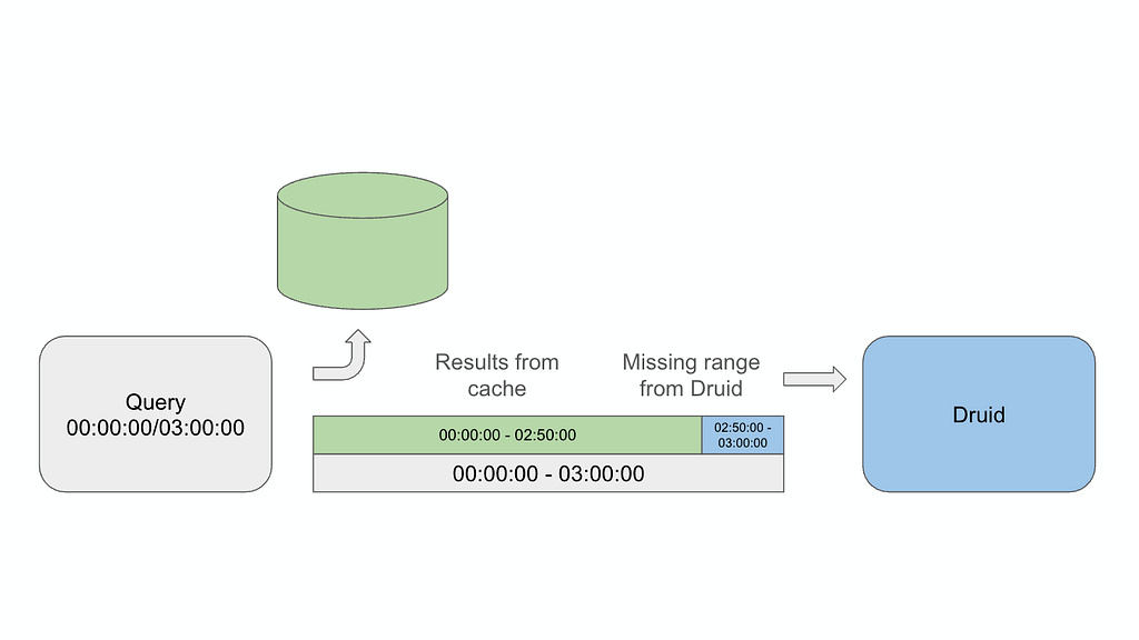
This is the core idea behind a new caching service that understands the structure of Druid queries and serves previously-seen results from cache while fetching only the freshest portion from Druid.
A Deliberate Trade-Off
Before diving into the implementation, it’s worth being explicit about the trade-off we’re making. Caching query results introduces some staleness, specifically, up to 5 seconds for the newest data. This is acceptable for most of our operational dashboards, which refresh every 10 to 30 seconds. In practice, many of our queries already set an end time of now-1m or now-5s to avoid the “flappy tail” that can occur with currently-arriving data.
Since our end-to-end data pipeline latency is typically under 5 seconds at P90, a 5-second cache TTL on the freshest data introduces negligible additional staleness on top of what’s already inherent in the system. We decided it was better to accept this small amount of staleness in exchange for significantly lower query load on Druid. But a 5s cache on its own is not very useful.
Exponential TTLs
Not all data points are equally trustworthy. In real-time analytics, there’s a well-known late-arriving data problem. Events can arrive out of order or be delayed in the ingestion pipeline. A data point from 30 seconds ago might still change as late-arriving events trickle in. A data point from 30 minutes ago is almost certainly final.
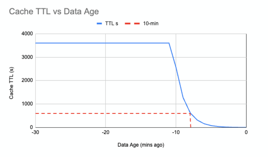
We use this observation to set cache TTLs that increase exponentially with the age of the data. Data less than 2 minutes old gets a minimum TTL of 5 seconds. After that, the TTL doubles for each additional minute of age: 10 seconds at 2 minutes old, 20 seconds at 3 minutes, 40 seconds at 4 minutes, and so on, up to a maximum TTL of 1 hour.
The effect is that fresh data cycles through the cache rapidly, so any corrections from late-arriving events in the most recent couple of minutes are picked up quickly. Older data lingers much longer, because our confidence in its accuracy grows with time.
For a 3-hour rolling window, the exponential TTL ensures the vast majority of the query is served from the cache, leaving Druid to only scan the most recent, unsettled data.
Bucketing
If we were to use a single-level cache key for the query and interval, similar to Druid’s existing result-level cache, we wouldn’t be able to extract only the relevant time range from cached results. A shifted window means a different key, which means a cache miss.
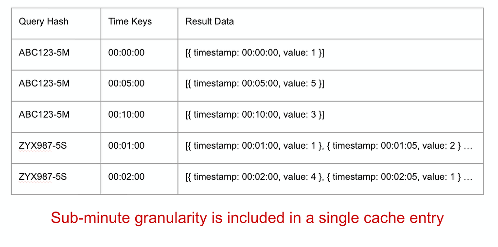
Instead, we use a map-of-maps. The top-level key is the query hash without the time interval; the inner keys are timestamps bucketed to the query granularity (or 1 minute, whichever is larger) and encoded as big-endian bytes so lexicographic order matches time. This enables efficient range scans; fetching all cached buckets between times A and B for a query hash. A 3-hour query at 1-minute granularity becomes 180 independent cached buckets, each with its own TTL; when the window shifts (e.g., 30 seconds later), we reuse most buckets from cache and only query Druid for the new data.
How It Works
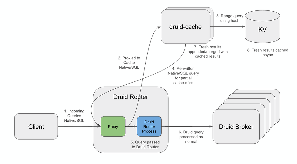
Today, the cache runs as an external service integrated transparently by intercepting requests at the Druid Router and redirecting them to the cache. If the cache fully satisfies a request, it returns the result; otherwise it shrinks the time interval to the uncached portion and calls back into the Router, bypassing the redirect to query Druid normally. Non-cached requests (e.g., metadata queries or queries without time group-bys) pass straight through to Druid unchanged.
This intercepting proxy design allows us to enable or disable caching without any client changes and is a key to its adoption. We see this setup as temporary while we work out a way to better integrate this capability into Druid more natively.
When a cacheable query arrives, those that are grouping-by time (timeseries, groupBy), the cache performs the following steps.
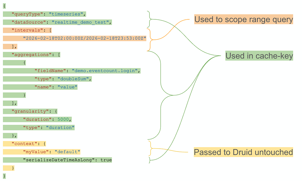
Parsing and Hashing. We parse each incoming query to extract the time interval, granularity, and structure, then compute a SHA-256 hash of the query with the time interval and parts of the context removed. That hash is the cache key: it encodes what is being asked (datasource, filters, aggregations, granularity) but not when, so the same logical query over different overlapping time windows maps to the same cache entry. There are some context properties that can alter the response structure or contents, so these are included in the cache-key.
Cache Lookup. Using the cache key, we fetch cached points within the requested range, but only if they’re contiguous from the start. Because bucket TTLs can expire unevenly, gaps can appear; when we hit a gap, we stop and fetch all newer data from Druid. This guarantees a complete, unbroken result set while sending at most one Druid query, rather than “filling gaps” with multiple small, fragmented queries that would increase Druid load.
Fetching the Missing Tail. On a partial cache hit (e.g., 2h 50m of a 3h window), we rebuild the query with a narrowed interval for the missing 10 minutes and send only that to Druid. Since Druid then scans just the recent segments for a small time range, the query is usually faster and cheaper than the original.
Combining. The cached data and fresh data are concatenated, sorted by timestamp, and returned to the client. From the client’s perspective, the response looks identical to what Druid would have returned, same JSON format, same fields.
Asynchronous Caching. The fresh data from Druid is parsed into individual time-granularity buckets and written back to the cache asynchronously, so we don’t add latency to the response path.
Negative Caching
Some metrics are sparse. Certain time buckets may genuinely have no data. Without special handling, the cache would treat these empty buckets as gaps and re-query Druid for them every time.
We handle this by caching empty sentinel values for time buckets where Druid returned no data. Our gap-detection logic recognizes these empty entries as valid cached data rather than missing data, preventing needless re-queries for naturally sparse metrics.
However, we’re careful not to negative-cache trailing empty buckets. If a query returns data up to minute 45 and nothing after, we only cache empty entries for gaps between data points, not after the last one. This avoids incorrectly caching “no data” for time periods where events simply haven’t arrived yet, which would exacerbate the chart delays of late arriving data.
The Storage Layer
For the backing store, we use Netflix’s Key-Value Data Abstraction Layer (KVDAL), backed by Cassandra. KVDAL provides a two-level map abstraction, a natural fit for our needs. The outer key is the query hash, and the inner keys are timestamps. Crucially, KVDAL supports independent TTLs on each inner key-value pair, eliminating the need for us to manage cache eviction manually.
This two-level structure gives us efficient range queries over the inner keys, which is exactly what we need for partial cache lookups: “give me all cached buckets between time A and time B for query hash X.”
Results
The biggest win is during high-volume events (e.g., live shows): when many users view the same dashboards, the cache serves most identical queries as full hits, so the query rate reaching Druid is essentially the same with 1 viewer or 100. The scaling bottleneck moves from Druid’s query capacity to the much cheaper-to-scale cache, and with ~5.5 ms P90 cache responses, dashboards load faster for everyone.
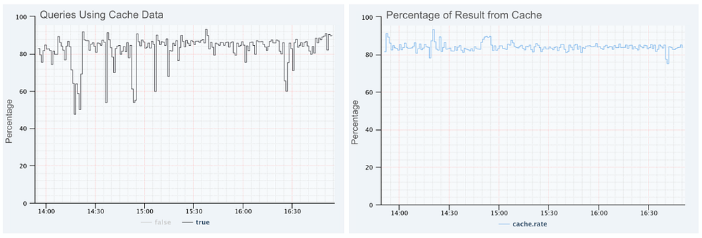
On a typical day, 82% of real user queries get at least a partial cache hit, and 84% of result data is served from cache. As a result, the queries that reach Druid scan much narrower time ranges, touching fewer segments and processing less data, freeing Druid to focus on aggregating the newest data instead of repeatedly re-querying historical segments.
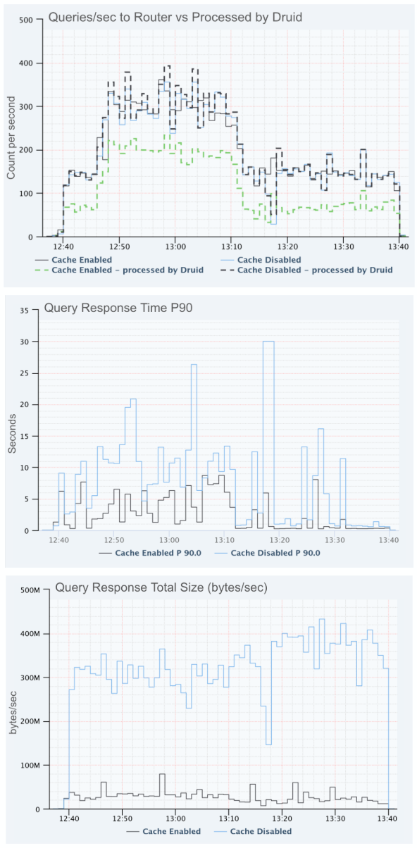
An experiment validated this, showing about a 33% drop in queries to Druid and a 66% improvement in overall P90 query times. It also cut result bytes and segments queried, and in some cases, enabling the cache reduced result bytes by more than 14x. Caveat: the size of these gains depends heavily on how similar and repetitive the query workload is.
Looking Ahead
This caching layer is still experimental, but results are promising and we’re exploring next steps. We’ve added partial support for templated SQL so dashboard tools can benefit without writing native Druid queries.
Longer term, we’d like interval-aware caching to be built into Druid: an external proxy adds infrastructure to manage, extra network hops, and workarounds (like SQL templating) to extract intervals. Implemented inside Druid, it could be more efficient, with direct access to the query planner and segment metadata, and benefit the broader community without custom infrastructure. We’d likely ship it as an opt-in, configurable, result-level cache in the Brokers, with metrics to tune TTLs and measure effectiveness. Please leave a comment if you have a use-case that could benefit from this feature.
More broadly, this strategy, splitting time-series results into independently cached, granularity-aligned buckets with age-based exponential TTLs, isn’t Druid-specific and could apply to any time-series database with frequent overlapping-window queries.
Summary
As more Netflix teams rely on real-time analytics, query volume grows too. Dashboards are essential at our scale, but their popularity can become a scaling bottleneck. By inserting an intelligent cache between dashboards and Druid, one that understands query structure, breaks results into granularity-aligned buckets, and trades a small amount of staleness for much lower Druid load, we’ve increased query capacity without scaling infrastructure proportionally, and hope to deliver these benefits to the Druid community soon as a built-in Druid feature.
Sometimes the best way to handle a flood of queries is to stop answering the same question twice.

Stop Answering the Same Question Twice: Interval-Aware Caching for Druid at Netflix Scale was originally published in Netflix TechBlog on Medium, where people are continuing the conversation by highlighting and responding to this story.
Unlock efficient model deployment: Simplified Inference Operator setup on Amazon SageMaker HyperPod
Post Syndicated from Shreya Gangishetty original https://aws.amazon.com/blogs/architecture/unlock-efficient-model-deployment-simplified-inference-operator-setup-on-amazon-sagemaker-hyperpod/
Amazon SageMaker HyperPod offers an end-to-end experience supporting the full lifecycle of AI development—from interactive experimentation and training to inference and post-training workflows. The SageMaker HyperPod Inference Operator is a Kubernetes controller that manages the deployment and lifecycle of models on HyperPod clusters, offering flexible deployment interfaces (kubectl, Python SDK, SageMaker Studio UI, or HyperPod CLI), advanced autoscaling with dynamic resource allocation, and comprehensive observability that tracks critical metrics like time-to-first-token, latency, and GPU utilization.
Deploying inference workloads on Kubernetes-native infrastructure has traditionally required AI teams to navigate a maze of Helm charts, IAM role configurations, dependency management, and manual upgrades — often taking hours before a single model can serve predictions. Today, we’re announcing the Amazon SageMaker HyperPod Inference Operator as a native EKS add-on, enabling one-click installation and managed upgrades directly from the SageMaker console. This eliminates the need for manual Helm charts, complex IAM configuration tweaks, and downtime during upgrades.
In this post, we walk through the new installation experience, demonstrate three deployment methods (console, CLI, and Terraform), and show how features like multi-instance-type deployment and native node affinity give you fine-grained control over inference scheduling
Simplified installation experience
The new installation experience addresses three key customer scenarios with streamlined workflows:
New HyperPod clusters: Automatic installation
When creating new HyperPod clusters through the SageMaker console’s Quick Setup or Custom Setup workflows, the Inference Operator along with necessary dependencies is now installed through EKS add-on automatically as part of the cluster creation process. This eliminates the need for post-deployment configuration and ensures your cluster is ready for model deployments immediately upon creation along with one click upgrades.
Existing clusters: One-click installation
For existing HyperPod clusters, customers can install the Inference Operator with a single click through the SageMaker console. The installation automatically:
- Creates required IAM roles with appropriate trust relationships and permissions
- Sets up S3 buckets for TLS certificate storage
- Configures VPC endpoints for secure S3 access
- Installs dependency add-ons (cert-manager, S3 CSI driver, FSx CSI driver, metrics-server)
- Deploys the Inference Operator as an EKS add-on
Managed upgrades and lifecycle
The EKS add-on integration provides standardized version management with one-click upgrades through the AWS console or CLI. This ensures customers can easily adopt new features and security updates without complex manual procedures.
The below prerequisite resources are needed to be setup before installing the Inference operator add-on. These prerequisites will be setup if SageMaker AI console is used to setup Inference operator. However, if EKS cli or console is used, these prerequisites will need to be created manually and passed to the add-on through configuration parameters. We discuss these approaches in Installation Methods.
List of prerequisites
- EKS add-ons (S3 Mountpoint csi driver add-on, FsX add-on, Cert Manager add-on, Metrics server add-on)
- IAM roles (Inference operator execution role, ALB role, KEDA role, Optional JumpStart Gated models role)
- Infrastructure (S3 bucket to manage TLS certificates, OIDC association on the cluster,
For more information refer to this trouble shooting guide.
Installation methods
Method 1: Install SageMaker HyperPod Inference Add-on through SageMaker UI (Recommended)
The SageMaker console provides the most streamlined experience with two installation options:
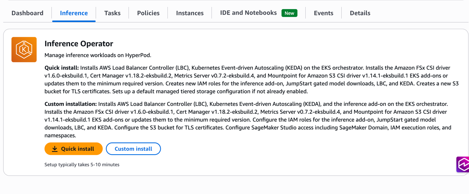
Quick install: Automatically creates all required resources with optimized defaults, including IAM roles, S3 buckets, and dependency add-ons. This option is ideal for getting started quickly with minimal configuration decisions.
Custom install: Provides flexibility to specify existing resources or customize configurations while maintaining the one-click experience. Customers can choose to reuse existing IAM roles, S3 buckets, or dependency add-ons based on their organizational requirements.
Prerequisites
- An existing Amazon SageMaker HyperPod cluster with EKS orchestration
- IAM permissions for EKS cluster administration
- kubectl configured for cluster access
Installation steps
- Navigate to the SageMaker Console: Go to HyperPod Clusters → Cluster Management
- Select Your Cluster: Choose the cluster where you want to install the Inference Operator
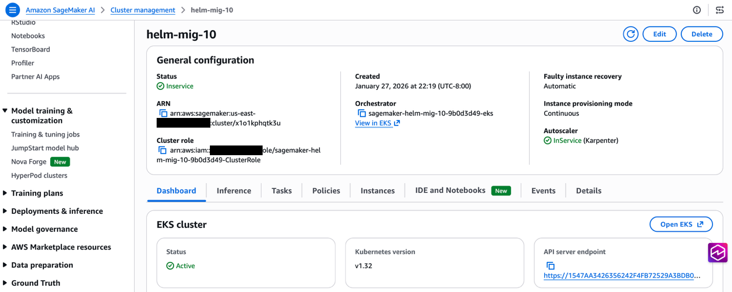
- Choose Installation Type: Navigate to Inference tab. Select Quick Install for automated setup or Custom Install for configuration flexibility
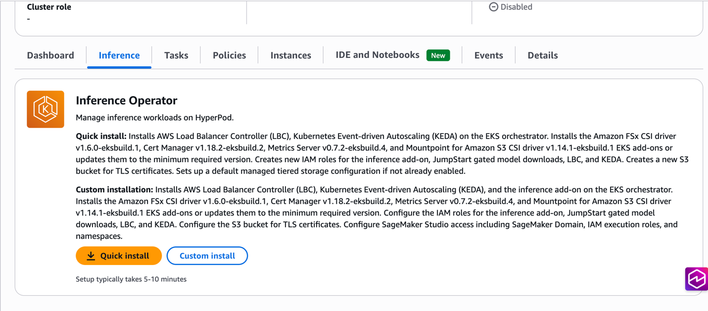
- Configure Options: If choosing Custom Install, specify existing resources or customize settings as needed
- Install: Choose Install to begin the automated installation process
- Verify: Check the installation status through the console, or by running
kubectl get pods -n hyperpod-inference-system, or by checking the add-on status withaws eks describe-addon --cluster-name CLUSTER-NAME --addon-name amazon-sagemaker-hyperpod-inference --region REGION
After the add-on is successfully installed, you can deploy models using the Model deployments document or navigate to Deploying Your First Model section below.
Method 2: Install SageMaker HyperPod Inference add-on through EKS APIs
For customers preferring command-line workflows, the Inference Operator can be installed directly using the EKS CLI. Note that all prerequisite resources (IAM roles, S3 buckets, VPC endpoints) and dependency add-ons must be created manually before installing the Inference Operator add-on. For detailed setup instructions, see the installation guide.
aws eks create-addon \
  --cluster-name my-hyperpod-cluster \
  --addon-name amazon-sagemaker-hyperpod-inference \
  --addon-version v1.0.0-eksbuild.1 \
  --configuration-values '{
    "executionRoleArn": "arn:aws:iam::ACCOUNT-ID:role/SageMakerHyperPodInference-inference-role",
    "tlsCertificateS3Bucket": "hyperpod-tls-certificate-bucket",
    "hyperpodClusterArn": "arn:aws:sagemaker:REGION:ACCOUNT-ID:cluster/CLUSTER-ID",
    "alb": {
      "serviceAccount": {
        "create": true,
        "roleArn": "arn:aws:iam::ACCOUNT-ID:role/alb-controller-role"
      }
    },
    "keda": {
      "auth": {
        "aws": {
          "irsa": {
            "roleArn": "arn:aws:iam::ACCOUNT-ID:role/keda-operator-role"
          }
        }
      }
    }
  }' \
  --region us-west-2
Method 3: Install SageMaker HyperPod Inference add-on through Terraform deployment
Organizations utilizing Terraform for Infrastructure as Code (IaC) can deploy HyperPod clusters using the provided modules in the awesome-distributed-training GitHub repository.
To enable the HyperPod inference operator, set the create_hyperpod_inference_operator_module variable to true within your custom.tfvars file, as shown below:
kubernetes_version    = "1.33"
eks_cluster_name      = "tf-eks-cluster"
hyperpod_cluster_name = "tf-hp-cluster"
resource_name_prefix  = "tf-eks-test"
aws_region            = "us-east-1"

instance_groups = [
    {
        name                      = "accelerated-instance-group-1"
        instance_type             = "ml.g5.8xlarge",
        instance_count            = 2,
        availability_zone_id      = "use1-az2",
        ebs_volume_size_in_gb     = 100,
        threads_per_core          = 1,
        enable_stress_check       = false,
        enable_connectivity_check = false,
        lifecycle_script          = "on_create.sh"
    }
]

create_hyperpod_inference_operator_module = true
In addition to the HyperPod inference operator add-on, the Terraform modules also support the task governance, training operator, and observability add-ons as well. Check out the documentation for enabling optional add-ons for more details.
Dependency management
The HyperPod inference operator includes several additional dependencies, which are enabled by default but can be toggled off if they already exist on your EKS cluster:
| Dependency | Module/Variable | Toggle to Disable |
| cert-manager | Installed via the HyperPod module | enable_cert_manager = false |
| Amazon FSx for Lustre CSI | Installed via FSx module | create_fsx_module = false |
| Mountpoint for Amazon S3 CSI | Bundled with Inference Operator Module | enable_s3_csi_driver = false |
| AWS Load Balancer Controller | Bundled with Inference Operator EKS add-on | enable_alb_controller = false |
| KEDA Operator | Bundled with Inference Operator EKS add-on | enable_keda = false |
Key benefits
Faster time to value
Teams can now deploy their first inference endpoint within minutes of cluster creation, compared to the previous multi-hour setup process. This acceleration enables faster experimentation and reduces the barrier to adoption for new teams.
Reduced complexity
The new installation experience eliminates the need to manually create and configure multiple AWS resources. Previously, customers needed to create IAM roles, policies, S3 buckets, VPC endpoints, and install multiple Kubernetes operators. Now, a single action handles all these requirements automatically.
Consistent configuration
Automated resource creation ensures consistent, secure configurations across environments. The installation process follows AWS best practices for IAM permissions, network security, and resource naming conventions.
Simplified upgrades
EKS Add-on integration provides standardized upgrade paths with rollback capabilities. Customers can confidently adopt new features and security updates through the familiar AWS console or CLI interfaces.
Advanced features integration
The simplified installation experience seamlessly integrates with advanced HyperPod inference capabilities:
Managed tiered KV cache
During installation, customers can optionally enable managed tiered KV cache with intelligent memory allocation based on instance types. This feature can reduce inference latency by up to 40% for long-context workloads while optimizing memory utilization across the cluster.
Intelligent routing
The installation automatically configures intelligent routing capabilities with multiple strategies (prefix-aware, KV-aware, round-robin) to maximize cache efficiency and minimize inference latency based on workload characteristics.
Observability integration
Built-in integration with HyperPod Observability provides immediate visibility into inference metrics, cache performance, and routing efficiency through Amazon Managed Grafana dashboards.
Deploying your first model
Once the add-on is installed, you can deploy models using the InferenceEndpointConfig or JumpStart models custom resources. Here’s an example configuration for deploying a Llama model:
apiVersion: inference.sagemaker.aws.amazon.com/v1
kind: JumpStartModel
metadata:
  name: deepseek-test-endpoint
spec:
  model:
    modelId: "deepseek-llm-r1-distill-qwen-1-5b"
  sageMakerEndpoint:
    name: deepseek-test-endpoint
  server:
    instanceType: "ml.g5.8xlarge"
New features
Multi-Instance Type Deployment HyperPod Inference supports multi-instance type deployment, enhancing deployment reliability and resource utilization. You can specify a prioritized list of instance types in your deployment configuration, and the system automatically selects from available alternatives when your preferred instance type lacks capacity. The Kubernetes scheduler evaluates instance types in priority order using node affinity rules based scheduling, seamlessly placing workloads on the highest-priority available instance type. In the example below, when deploying a model from S3, ml.p4d.24xlarge has the highest priority and will be selected first if memory capacity is available. If ml.p4d.24xlarge is unavailable, the scheduler automatically falls back to ml.g5.24xlarge, and finally to ml.g5.8xlarge as the last resort.
apiVersion: inference.sagemaker.aws.amazon.com/v1
kind: InferenceEndpointConfig
metadata:
  name: lmcache-test-1
  namespace: default
spec:
  replicas: 13
  modelName: Llama-3.1-8B-Instruct
  instanceTypes: ["ml.p4d.24xlarge","ml.g5.24xlarge","ml.g5.8xlarge"]
This is implemented using Kubernetes node affinity rules with requiredDuringSchedulingIgnoredDuringExecution to restrict scheduling to the specified instance types, and preferredDuringSchedulingIgnoredDuringExecution with descending weights to enforce priority ordering.
Node affinity
For scenarios requiring more granular scheduling control — such as excluding spot instances, preferring specific availability zones, or targeting nodes with custom labels — HyperPod Inference exposes Kubernetes’ native nodeAffinity directly in the InferenceEndpointConfig spec. This gives you the full expressiveness of Kubernetes scheduling primitives.
apiVersion: inference.sagemaker.aws.amazon.com/v1
kind: InferenceEndpointConfig
metadata:
  name: lmcache-test-1
  namespace: default
spec:
  replicas: 15
  modelName: Llama-3.1-8B-Instruct
  nodeAffinity:
    preferredDuringSchedulingIgnoredDuringExecution:
    - weight: 100
      preference:
        matchExpressions:
        - key: node.kubernetes.io/instanceType
          operator: In
          values: ["ml.g5.4xlarge"]
  worker:
    resources:
      limits:
        nvidia.com/gpu: "1"
      requests:
        cpu: "6"
        memory: 30Gi
        nvidia.com/gpu: "1"
Clean up
To clean up your environment after completing this walkthrough, follow these steps to remove the deployed models and uninstall the Inference Operator add-on from your HyperPod cluster.
Removing Inference Operator add-on
Through the SageMaker console:
- Navigate to SageMaker Console → HyperPod Clusters → Cluster Management
- Select your cluster and go to the Inference tab
- Choose Remove to uninstall the Inference Operator add-on and associated resources
Alternatively, using the AWS CLI:
aws eks delete-addon \
--cluster-name <my-hyperpod-cluster> \
--addon-name amazon-sagemaker-hyperpod-inference \
--region <region>
Delete the deployed models
# Delete JumpStartModel deployment
kubectl delete jumpstartmodel <model-name> -n <namespace>

# Or for InferenceEndpointConfig deployment
kubectl delete inferenceendpointconfig <endpoint-name> -n <namespace>
Migration path for existing users
Automated migration script is hosted in public GitHub that transitions the HyperPod Inference Operator from Helm to EKS add-on with built-in rollback capabilities if add-on installation fails. Backup files are stored in /tmp/hyperpod-migration-backup-<timestamp>/ for manual rollback if needed.
Key features
- Auto-Discovery: Derives configuration from existing Helm deployment (roles, buckets, dependencies)
- Safe Migration: Scales down Helm deployments before add-on installation, validates prerequisites
- Dependency Handling: Migrates S3/FSx CSI drivers, cert-manager, and metrics-server to add-ons
- Rollback Support: Preserves original resources and restores on failure
IAM Roles created
- Execution Role (Inference Operator + S3 TLS access)
- JumpStart Gated Model Role
- ALB Controller Role
- KEDA Operator Role
Examples for running the script
# to follow step by step guide
./helm_to_addon.sh --cluster-name <my-cluster> --region us-east-1

# no prompts needed except for initiating rollback in case of failure
./helm_to_addon.sh --cluster-name <my-cluster> --region us-east-1 --auto-approve

# To skip the dependencies FSX, S3, Metricsserver, cert manager migration from Inference operator helm to respective add-ons
./helm_to_addon.sh --cluster-name my-cluster —region us-east-1 --skip-dependencies-migration
Migration flow
- Validate existing Helm installation
- Auto-derive configuration and create new IAM roles
- Tag resources (ALBs, ACM certs, S3 objects) with
CreatedBy: HyperPodInference - Install dependency add-ons (S3, FSx, cert-manager) if dependent CRDs don’t exist
- Scale down Helm deployments for ALB, KEDA and Inference operator
- Install Inference Operator add-on with
OVERWRITEflag - Clean up old Helm resources
- Migrate Helm-installed dependencies that are installed through Inference operator main chart to add-ons. To skip this step provide
--skip-dependenciesflag.
Benefits
- Simplified management through EKS console/APIs
- Automated updates via EKS add-on mechanisms
- Native EKS integration
- Zero downtime migration with rollback safety
Conclusion
The streamlined Inference Operator installation experience for Amazon SageMaker HyperPod eliminates infrastructure complexity and accelerates time to value for machine learning teams. With one-click installation, automated resource management, and seamless upgrade capabilities, teams can focus on deploying and optimizing their inference workloads rather than managing underlying infrastructure.
The EKS Add-on integration provides enterprise-grade lifecycle management while maintaining the flexibility to customize configurations for specific organizational requirements. Combined with advanced features like managed tiered KV cache and intelligent routing, this simplified installation experience makes high-performance inference deployment accessible to teams of all sizes.
Get started today by creating a new HyperPod cluster with the Inference Operator pre-installed, or add it to your existing clusters with a single click through the SageMaker console. For detailed add-on installation instructions and configuration options see this guide and for troubleshooting see this guide.
Appendix
About the authors
How we built Organizations to help enterprises manage Cloudflare at scale
Post Syndicated from Justin Hutchings original https://blog.cloudflare.com/organizations-beta/
Cloudflare was designed to be simple to use for even the smallest customers, but it’s also critical that it scales to meet the needs of the largest enterprises. While smaller customers might work solo or in a small team, enterprises often have thousands of users making use of Cloudflare’s developer, security, and networking capabilities. This scale can add complexity, as these users represent multiple teams and job functions.
Enterprise customers often use multiple Cloudflare Accounts to segment their teams (allowing more autonomy and separation of roles), but this can cause a new set of problems for the administrators by fragmenting their controls.
That’s why today, we’re launching our new Organizations feature in beta — to provide a cohesive place for administrators to manage users, configurations, and view analytics across many Cloudflare Accounts.
The principle of least privilege is one of the driving factors behind enterprises using multiple accounts. While Cloudflare’s role-based access control (RBAC) system now offers fine-grained permissions for many resources, it can be cumbersome to enumerate all the resources one by one. Instead, we see enterprises use multiple accounts, so each team’s resources are managed by that team alone. This allows organic growth within the account: they can add new resources as needed, without giving Administrative control too widely.
While multiple accounts are great at limiting permissions for most of the users within an organization, they complicate things for the administrators, as the administrators need to be added to every account and given the appropriate permissions to handle tasks like reporting or setting policies. This situation is fragile, as other administrators could remove them.
We designed Cloudflare Organizations with these scenarios in mind. Organizations adds a new layer to the hierarchy so that administrators can manage a collection of accounts together. Organizations is built on top of the Tenant system, which we created to support the needs of Cloudflare’s partner ecosystem. This provides a strong foundation for the many new features we’ve built with enterprises in mind.
The account list is at the core of the organization. This is a flat list of all the accounts that have been onboarded to the organization. “Org Super Administrator” is a new user role that is managed at the organization level; users with this role can add more accounts to the list as long as they are a Super Administrator of the account as well.
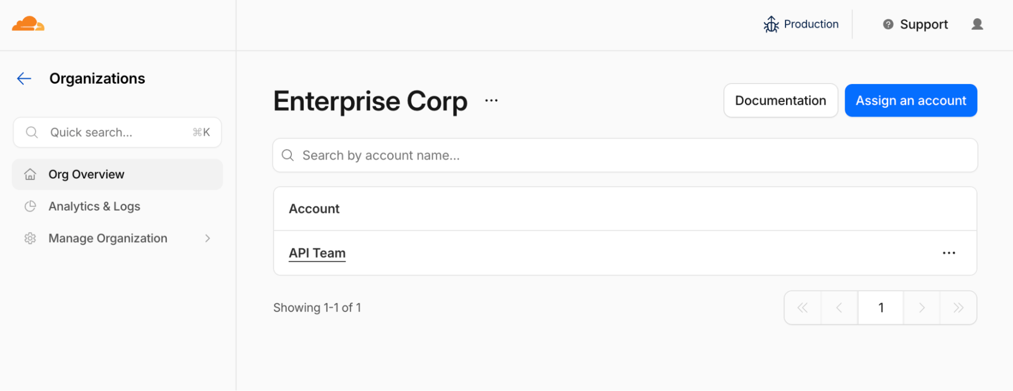
Org Super Administrators have Super Administrator permissions to every account in the organization. They do not require a membership in any of the child accounts and will not be listed in the account level UI. Org Super Administrator is the first of many roles we anticipate adding at the organization layer over the course of the year.
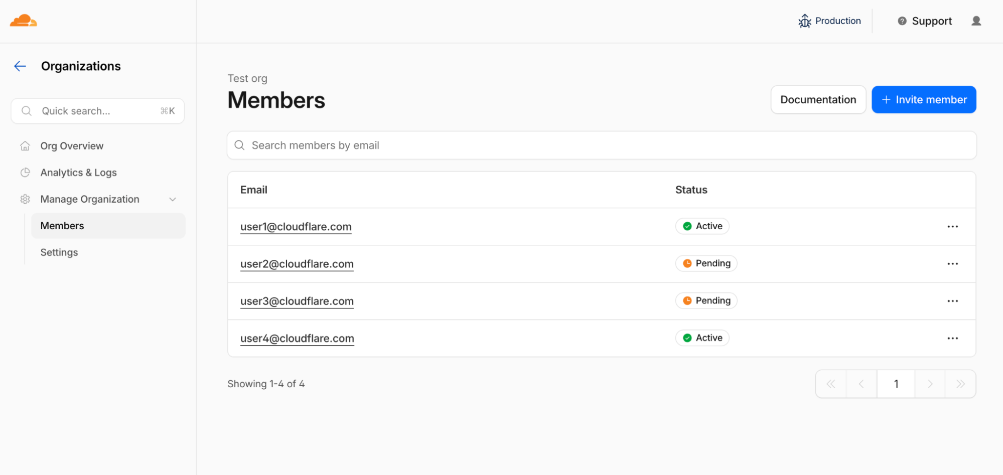
This feature was the culmination of a major innersource development project that we ran within the organization to remove legacy codepaths and consolidate every authorization check on our domain-scoped roles system. We added almost 133,000 lines of new code and removed about 32,000 lines of old code in support of this, making it one of the largest changes to our permissions system ever. This foundational improvement will make it easier to deliver additional roles in the future, both at the organization and account levels. We also made a 27% performance improvement in how we check permissions on enumeration calls like /accounts or /zones, which previously struggled with users that have access to thousands of accounts.
Org super administrators can view a roll-up dashboard complete with analytics about their HTTP traffic from across all accounts and zones. HTTP traffic analytics is the first of many analytics dashboards that we expect to deliver over the course of the year as we add this feature for more products.

Managing shared policies across your organization allows one team to centrally manage features like WAF (Web Application Firewall) or Gateway policies. Org Super Administrators will have the ability to share a policy set from one account to the rest of the accounts within the organization. That means any users in the source account with permission to manage those configurations can update the policy sets. So security analysts can update WAF rules for an entire enterprise centrally, without needing to be org administrators or administrators of other accounts in the organization.
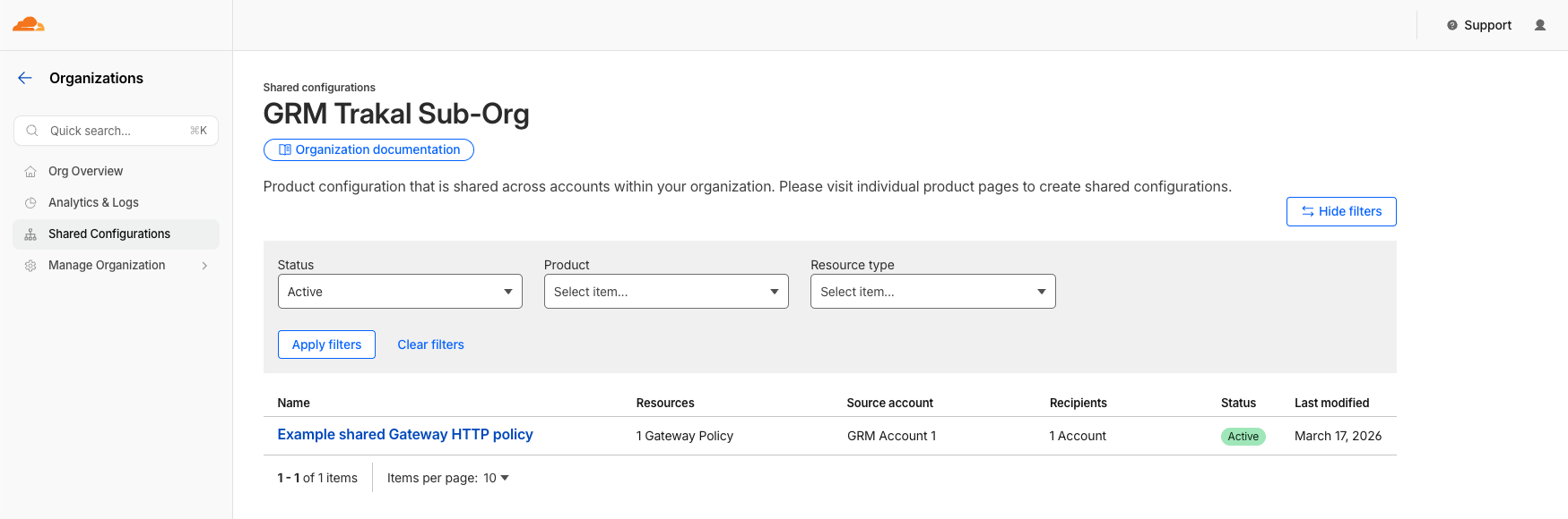
We’ve limited the initial launch of Organizations only to enterprise customers, but will be expanding it to all customers in the coming months starting with pay-as-you-go customers. We’ll be working to extend this to our partner ecosystem too, but have a number of special scenarios we need to address for them before we do.
There’s a lot more on the roadmap in this space. Keep an eye on the changelog for capabilities coming soon:
- Organization-level audit logs
- Organization-level billing reports
- More organization-level analytics reports
- Additional organization user roles
- Self-serve account creation
Organizations is rolling out in public beta over the next several days to enterprise customers. In introducing Organizations, our own key requirements are that we do not elevate privilege for any users, and that customers create just one organization each. To deliver on those requirements, we elected not to do a backfill and create organizations on your behalf, and are instead using a self-serve invitation process.
If you are a Super Administrator of an enterprise account, and nobody else has created an organization for your company, then you will see an invitation to create an organization in your Cloudflare dashboard. Once you have created an organization, you can add accounts to the organization if you are a super administrator of that account as well.
If another user in your company has already claimed the organization, then they can either invite you as an Org Super Administrator so that you can add your accounts to the organization, or you can invite them as a Super Administrator of your account, so they can add your account to the organization. This process ensures that no user ever gets permission to a Cloudflare account where a Super Administrator was not involved in approving it. Cloudflare support will not be making configuration changes on behalf of customers, so plan to work with other administrators to complete your internal rollout of Organizations.
If you’re a Super Administrator of an enterprise account, claim your company’s organization now. There is no additional fee for using Organizations. You can find more details on how to get started in the Dashboard under the new Organizations tab, or at our developer docs.
If you’re not an enterprise customer, keep an eye on our changelog for more information about when Organizations will be available for your plan. And to learn more about our enterprise offerings, our enterprise sales team can get you started today.
Introducing the FreeBSD laptop integration testing project
Post Syndicated from jzb original https://lwn.net/Articles/1066593/
Recently, the FreeBSD Foundation has been making
progress on improving the operating system’s support for modern
laptop hardware. The foundation is now looking to expand testing to
encompass a wider range of hardware; it has announced
a laptop integration testing project to allow the community to easily
test FreeBSD’s compatibility with laptops and submit the results.
With limited access to testing systems, there’s only so much we can
do! We hope to work together with volunteers from the community who
want FreeBSD to work well on their laptops.While we expect device hardware and software enumeration to be a
fully automated process, we feel that manually-submitted comments
about personal experience with FreeBSD are equally valuable. We plan
to highlight this commentary on our “matrix of compatibility” webpage
for each tested laptop.We are striving to make it as easy as possible to submit your
results. You won’t have to worry about environment setup, submission
formatting, or any repo-specific details!
See the project
repository and testing
instructions for more.
New Mexico’s Meta Ruling and Encryption
Post Syndicated from Bruce Schneier original https://www.schneier.com/blog/archives/2026/04/new-mexicos-meta-ruling-and-encryption.html
Mike Masnick points out that the recent New Mexico court ruling against Meta has some bad implications for end-to-end encryption, and security in general:
If the “design choices create liability” framework seems worrying in the abstract, the New Mexico case provides a concrete example of where it leads in practice.
One of the key pieces of evidence the New Mexico attorney general used against Meta was the company’s 2023 decision to add end-to-end encryption to Facebook Messenger. The argument went like this: predators used Messenger to groom minors and exchange child sexual abuse material. By encrypting those messages, Meta made it harder for law enforcement to access evidence of those crimes. Therefore, the encryption was a design choice that enabled harm.
The state is now seeking court-mandated changes including “protecting minors from encrypted communications that shield bad actors.”
Yes, the end result of the New Mexico ruling might be that Meta is ordered to make everyone’s communications less secure. That should be terrifying to everyone. Even those cheering on the verdict.
End-to-end encryption protects billions of people from surveillance, data breaches, authoritarian governments, stalkers, and domestic abusers. It’s one of the most important privacy and security tools ordinary people have. Every major security expert and civil liberties organization in the world has argued for stronger encryption, not weaker.
But under the “design liability” theory, implementing encryption becomes evidence of negligence, because a small number of bad actors also use encrypted communications. The logic applies to literally every communication tool ever invented. Predators also use the postal service, telephones, and in-person conversation. The encryption itself harms no one. Like infinite scroll and autoplay, it is inert without the choices of bad actors - choices made by people, not by the platform’s design.
The incentive this creates goes far beyond encryption, and it’s bad. If any product improvement that protects the majority of users can be held against you because a tiny fraction of bad actors exploit it, companies will simply stop making those improvements. Why add encryption if it becomes Exhibit A in a future lawsuit? Why implement any privacy-protective feature if a plaintiff’s lawyer will characterize it as “shielding bad actors”?
And it gets worse. Some of the most damaging evidence in both trials came from internal company documents where employees raised concerns about safety risks and discussed tradeoffs. These were played up in the media (and the courtroom) as “smoking guns.” But that means no company is going to allow anyone to raise concerns ever again. That’s very, very bad.
In a sane legal environment, you want companies to have these internal debates. You want engineers and safety teams to flag potential risks, wrestle with difficult tradeoffs, and document their reasoning. But when those good-faith deliberations become plaintiff’s exhibits presented to a jury as proof that “they knew and did it anyway,” the rational corporate response is to stop putting anything in writing. Stop doing risk assessments. Stop asking hard questions internally.
The lesson every general counsel in Silicon Valley is learning right now: ignorance is safer than inquiry. That makes everyone less safe, not more.
The essay has a lot more: about Section 230, about competition in this space, about the myopic nature of the ruling. Go read it.
The Manosphere Turns on Trump
Post Syndicated from The Atlantic original https://www.youtube.com/shorts/HyBik5FcXJE
Modernize business intelligence workloads using Amazon Quick
Post Syndicated from Satesh Sonti original https://aws.amazon.com/blogs/big-data/modernize-business-intelligence-workloads-using-amazon-quick/
Traditional business intelligence (BI) integration with enterprise data warehouses has been the established pattern for years. With generative AI, you can now modernize BI workloads with capabilities like interactive chat agents, automated business processes, and using natural language to generate dashboards.
In this post, we provide implementation guidance for building integrated analytics solutions that combine the generative BI features of Amazon Quick with Amazon Redshift and Amazon Athena SQL analytics capabilities. Use this post as a reference for proof-of-concept implementations, production deployment planning, or as a learning resource for understanding Quick integration patterns with Amazon Redshift and Athena.
Common use cases
You can use this integrated approach across several scenarios. The following are some of the most common use cases.
- Traditional BI reporting benefits from bundled data warehouse and BI tool pricing, making generative BI the primary use case with significant cost advantages.
- Insurance: Automates Solvency II and IFRS 17 regulatory reporting, replacing manual spreadsheet consolidation.
- Banking: Accelerates FDIC call report generation and capital adequacy dashboards, cutting month-end close from days to hours.
- Interactive dashboards with contextual chat agents give BI teams conversational interfaces alongside their visual metrics.
- Gaming: Live ops teams query player retention and monetization KPIs in plain English—no SQL needed.
- Financial Services: Trading analysts chat with real-time P&L dashboards to surface anomalies and drill into positions on demand.
- Domain-specific analytics workspaces democratize enterprise data exploration through Quick Spaces and natural language queries.
- Insurance: Actuarial and underwriting teams query claims and risk data without waiting on data engineering.
- Banking: Risk and compliance teams explore credit, market, and operational data through a single natural language interface.
- Workflow automation removes repetitive tasks and accelerates self-service analytics.
- Financial Services: Automated AR reconciliation flows replace manual ledger matching, shrinking close cycle effort significantly.
- Gaming: Telemetry ingestion pipelines trigger reporting refreshes automatically, freeing data engineers from routine work.
Let us examine an end-to-end solution combining these technologies.
Solution flow
AWS offers two native SQL analytics engines for building analytics workloads. Amazon Redshift provides a fully managed data warehouse with columnar storage and massively parallel processing. Amazon Athena delivers serverless interactive query capabilities directly against data in Amazon S3.
You can use either Amazon Redshift or Amazon Athena as a SQL engine while implementing the steps in this post. The following are the steps involved in building an end-to-end solution.
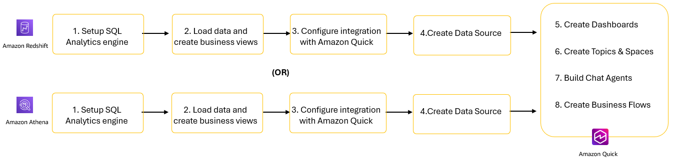
Figure1: Solution steps to integrate SQL Analytics engines with Amazon Quick
- Set up your SQL analytics engines: Amazon Redshift or Amazon Athena.
- Load data and create business views designed for analytics workloads.
- Configure integration between SQL analytics engines and Amazon Quick.
- Create data sources in Amazon Quick.
- Create datasets and dashboards for visual analytics.
- Use Topics and Spaces to provide natural language interfaces to your data.
- Deploy chat agents to deliver conversational AI experiences for business users.
- Implement business flows to automate repetitive workflows and processes.
Let’s start by walking through steps 1–4 for Amazon Redshift. We then describe the same four steps for Amazon Athena before explaining the Amazon Quick steps 5–8.
Configure and create datasets in Amazon Redshift
Amazon Redshift offers two deployment options to meet your data warehousing needs. Provisioned clusters provide traditional deployment where you manage compute resources by selecting node types and cluster size. Serverless automatically scales compute capacity based on workload demands with pay-per-use pricing. Both options are supported by Amazon Quick. For this walkthrough, we use Redshift Serverless.
Set up SQL analytics engine
To create a Redshift Serverless namespace and workgroup:
- Open the Amazon Redshift console.
- On the left navigation pane, select Redshift Serverless.
- Follow the steps described in the Creating a workgroup with a namespace documentation page to create a workgroup and a namespace. Note the username and password provided. You will use these details for configuring connections in Amazon Redshift and Quick.
- You should see the status as Available for both the workgroup and namespace in the Serverless dashboard.
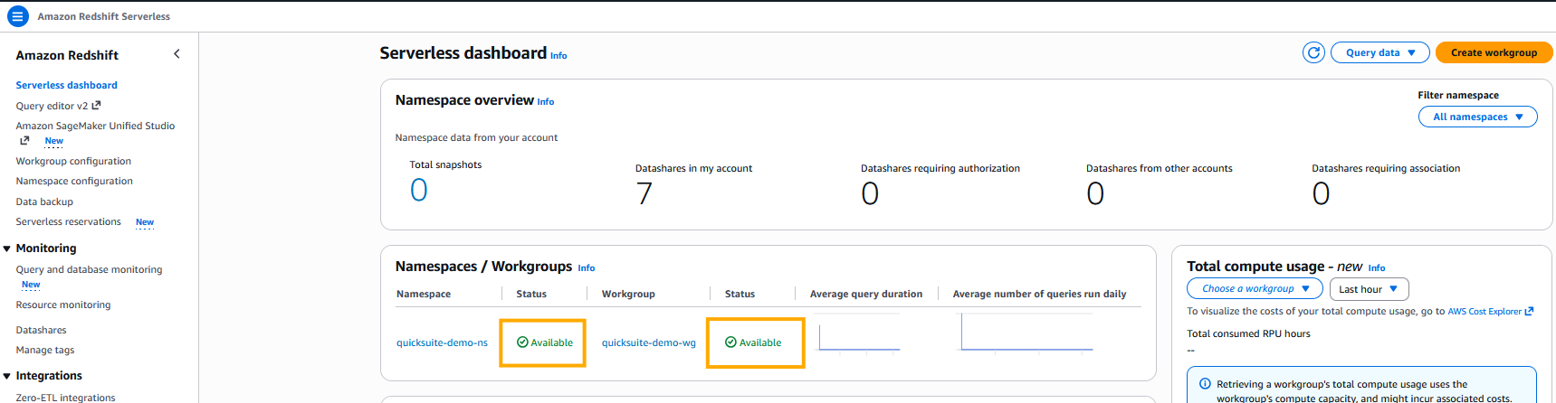
Figure 2: Amazon Redshift Serverless Workgroup and NamespacesThe deployment will be completed in approximately 3–5 minutes.
Load data and create business views
Now you can load data using the industry-standard TPC-H benchmark dataset, which provides realistic customer, order, and product data for analytics workloads.To load data into Amazon Redshift:
- Open the Amazon Redshift Query Editor V2 from the console.
- Run the TPC H DDL statements to create TPC-H tables.
- Run the following COPY commands to load data from the public S3 bucket:
s3://redshift-downloads/TPC-H/.
Ensure that the IAM role attached to the namespace is set as the default IAM role. If you didn’t set up the default IAM role at the time of namespace creation, you can refer to the Creating an IAM role as default for Amazon Redshift documentation page to set it now.
Run the following query to validate load status. The status column should show as completed. You can also review the information in other columns to see details about the loads such as record counts, duration, and data source.

Figure 3: Output of SYS_LOAD_HISTORY showing successful completion of COPY Jobs
- Create a materialized view to improve query performance:
Run the following SQL to create a materialized view that pre-compute results set for customer revenues and order volumes by market segment.
Run the following SQL to review the data in the materialized view.
Configure integration with Amazon Quick
Amazon Quick auto discovers the Amazon Redshift provisioned clusters that are associated with your AWS account. These resources must be in the same AWS Region as your Amazon Quick account. For Amazon Redshift clusters in other accounts or Amazon Redshift Serverless, we recommend that you add a VPC connection following the steps in Enabling access to an Amazon Redshift cluster in a VPC documentation. Usually, these steps are performed by your organization’s cloud security administration team.
For serverless, you will apply the same steps in the workgroup instead of the cluster. You can find the VPC and Security Group settings in the Data Access tab of a workgroup.
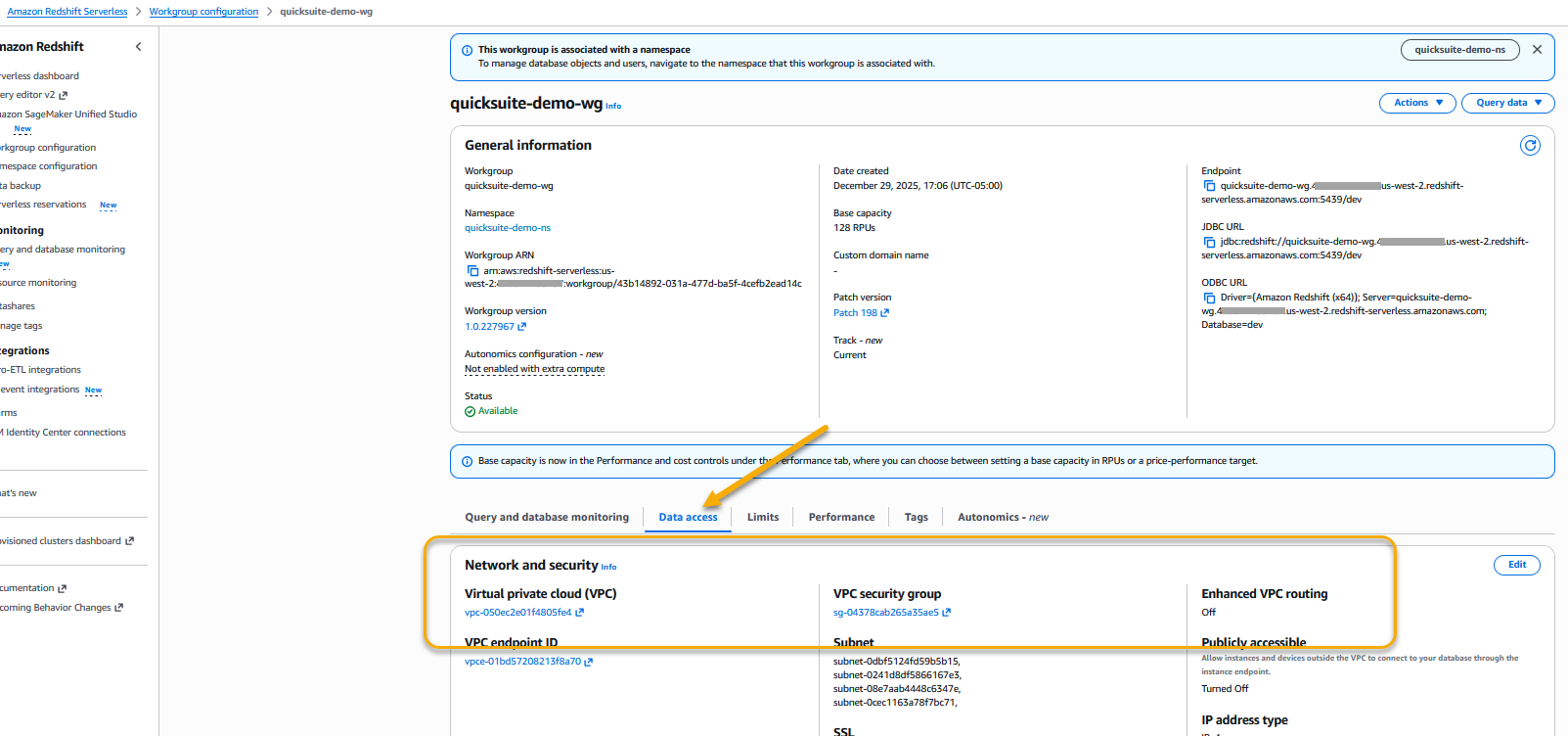
Figure 4: Amazon Redshift Serverless workgroup VPC and Security groups
You can also refer to How do I privately connect Quick to an Amazon Redshift or RDS data source in a private subnet? for a demonstration.
Create data source
To create a dataset connecting to Amazon Redshift, complete the following steps.
- In the Quick left navigation pane, go to Datasets.
- Choose the Data sources tab and select Create data source.
- Select Amazon Redshift and enter the following:
- Data Source Name: Provide
customer-rev-datasourceas data source name. - Connection type: Select the VPC connection created in the previous step.
- Database server: Enter the Amazon Redshift workgroup endpoint (for example,
quick-demo-wg.123456789.us-west-2.redshift-serverless.amazonaws.com). - Port: 5439 (default).
- Database:
dev. - Username/Password: Amazon Redshift credentials with access to the database.
- Data Source Name: Provide
- Choose Validate connection. The validation should be successful.
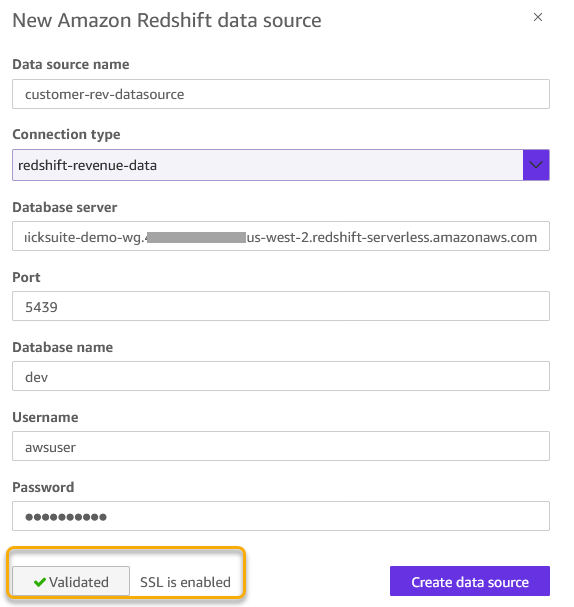
Figure 5: Amazon Redshift data source configuration
- Choose Create Data Source to create a data source.
Now let’s explore how to perform all these four steps to configure Athena in Amazon Quick.
Configure and create datasets in Amazon Athena
Amazon Athena provides immediate query capabilities against petabytes of data with automatic scaling to handle concurrent users. Let’s go through the steps to configure connections between Amazon Quick and Amazon Athena.
Set up SQL analytics engine
To create an Athena workgroup:
- Open the Amazon Athena console.
- In the navigation pane, choose Workgroups.
- Choose Create workgroup.
- For Workgroup name, enter
quick-demo. - For Query result configuration, select Athena managed.
- Choose Create workgroup.
Your workgroup is ready immediately for querying data.
Load data and create business views
For Athena, you create tables using the TPC-H benchmark dataset that AWS provides in a public S3 bucket. This approach gives you 1.5 million customer records already optimized in Parquet format without requiring data loading.
To create tables and views in Athena:
- Open the Athena Query Editor from the console.
- Create a database for your analytics (create S3 bucket if it exists already):
- Create an external table pointing to the TPC-H public dataset:
- Create a business-friendly view for analytics:
Run the following SQL to create a view that aggregates customer account balances grouped by market segments.
- Verify your view from Athena with:
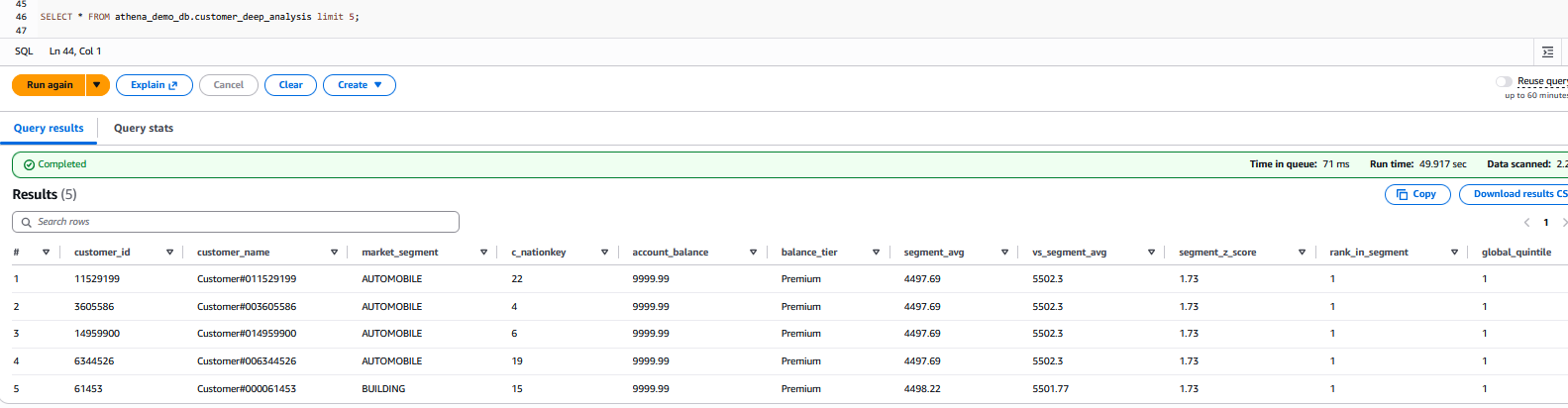
Figure 6: Output from the SELECT query
Configure integration with Amazon Quick
To connect to Amazon Athena in Amazon Quick, follow these steps, consolidated from official AWS documentation and authorizing connections to Amazon Athena.
Authorize Quick to Access Athena, S3 Bucket for data, and S3 bucket for Athena Results.
Open the Amazon Quick Security Settings
- Sign in to the Amazon Quick console as an administrator.
- In the top-right corner, choose your profile icon, then select Manage account.
- Under Permissions, choose AWS resources.

Figure 7: AWS resource permissions
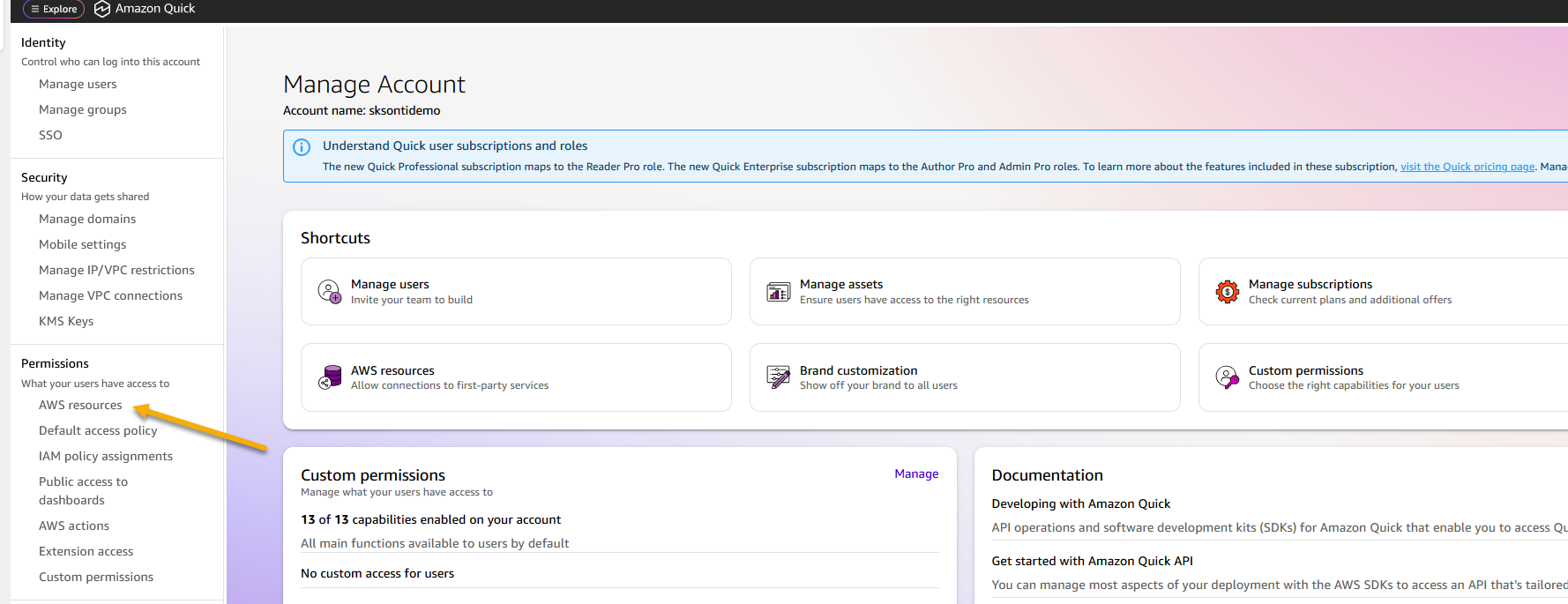
Enable Athena Access
- Under Quick access to AWS services, choose Manage.
- Locate Amazon Athena in the list of AWS services.
- If Athena is already selected but access issues persist, clear the checkbox and re-select it to re-enable Athena.
- Under Amazon S3, select S3 buckets.
- Check the boxes next to each S3 bucket that Amazon Quick needs to access—including buckets used for Athena query results and any Redshift COPY source buckets.
- Enable Write permission for Athena Workgroup to allow Amazon Quick to write Athena query results to S3 and choose Finish.
- Choose Save to update the configuration.
The final step is to grant your Amazon Quick author permissions to query your database, Athena tables, and views. Configuration depends on whether AWS Lake Formation is enabled.
If AWS Lake Formation is not enabled
Permissions are managed at the Quick service role level through standard IAM-based S3 access control. Ensure that the Quick service role (for example, aws-quick-service-role-v0) has the appropriate IAM permissions for the relevant S3 buckets and Athena resources. No additional Lake Formation configuration is required.
If AWS Lake Formation is enabled
Lake Formation acts as the central authorization layer, overriding standard IAM-based S3 permissions. Grant permissions directly to the Amazon Quick author or IAM role.
To grant data permissions:
- Open the AWS Lake Formation console.
- Choose Permissions, then Data permissions, then Grant.
- Select the IAM user or role.
- Choose the required databases, tables, and columns.
- Grant SELECT at minimum; add DESCRIBE for dataset creation.
- Repeat for each user or role that requires access.
Create data source
Follow these steps to create an Athena data source on Amazon Quick.
- In the Amazon Quick console, navigate to Datasets and choose Data sources tab.
- Choose Create data source, then select the Amazon Athena card.
- Enter a Data source name (you can give any name of your choice), select your Athena workgroup (like quick-demo), and choose Validate connection.
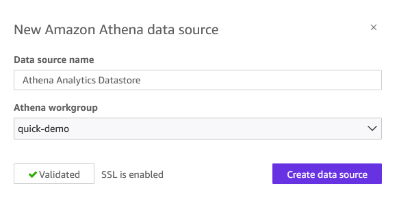
Figure 8: Athena data source creation
- Choose Create data source.
Your Athena data source is now available for building datasets, dashboards, and Topics.
Use Amazon Quick generative AI features
The next steps, from 5–8, demonstrate Amazon Quick generative AI capabilities using Amazon Redshift as a data source. While we use Amazon Redshift in this example, you can substitute with Amazon Athena based on your specific requirements.
Create dashboards
Let’s start by creating datasets from the Amazon Redshift data source.
- In the left navigation pane, choose Datasets.
- On the Datasets page, choose Create Dataset.
- For the data source, select Amazon Redshift data source
customer-rev-datasource. - From the menu, choose
mv_customer_revenue.
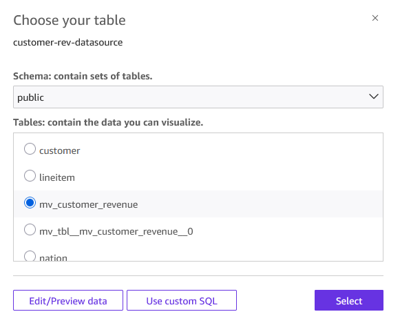
Figure 9: Select table to visualize
- You can choose one of the following query modes. For this post, select Directly query your data option and choose Visualize.
- Import to SPICE for quicker analytics – Quick loads a snapshot into its in-memory engine for faster dashboard performance.
- Directly query your data– Quick runs queries on demand against your query engine.
- Select Build icon to open a chat window. Enter “Show me orders by market segments” as the prompt. Note that you need Author Pro access to use this feature.
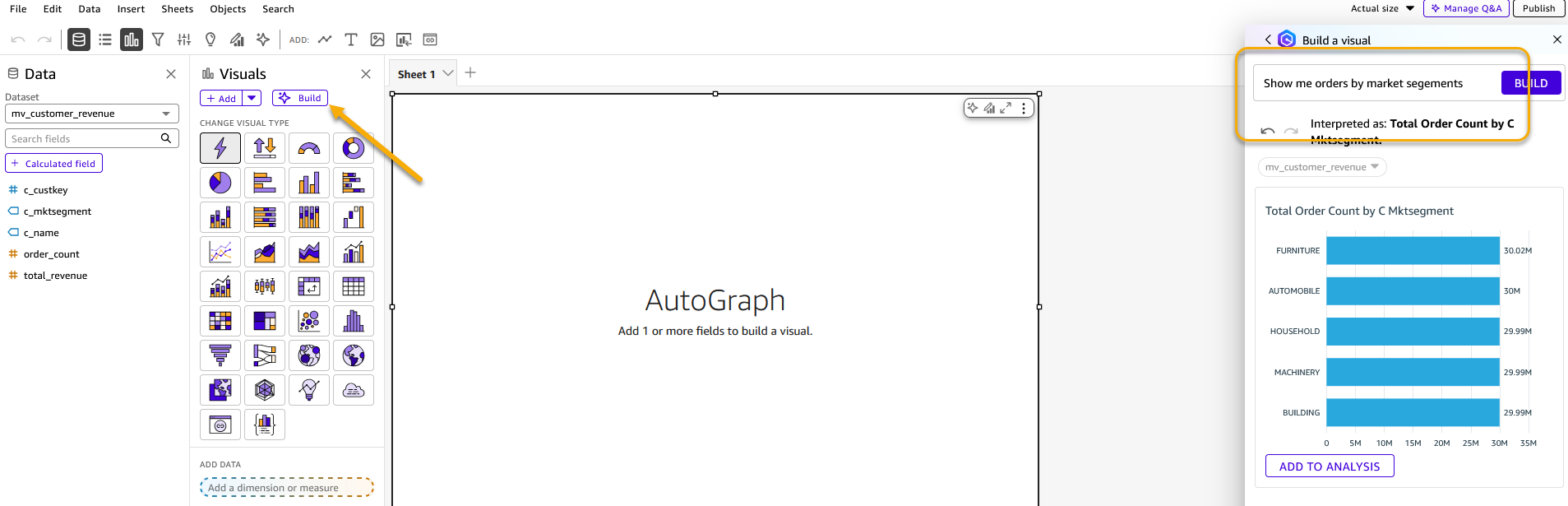
Figure 10: Build visualization using generative BI feature
- You can change the visual type to a pie chart and add it to the analysis.
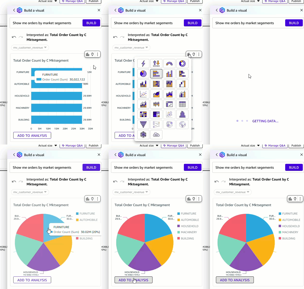
Figure 10: Change visual type
To publish your analysis as a dashboard
- After you add the visuals, choose Publish.
- Enter a name for the dashboard. For this post, use the Market Segment Dashboard.
- Choose Publish dashboard. Your dashboard is now available for viewing and sharing.
Create topics and spaces
To fully maximize enterprise data with AI, we must provide the right structure and context. That’s where Topics and Spaces come in. Topics act as natural language interfaces to your structured datasets, automatically analyzing your data, mapping fields, and adding synonyms. Business users can ask “What are total revenues by market segment?” and receive instant, visualized answers without writing a single line of SQL. Spaces bring together all of your related assets into a single collaborative workspace that democratizes data access, reduces context-switching, accelerates team onboarding, so everyone is working from the same trusted, AI-ready data sources.
To create a Quick topic
- From the Amazon Quick homepage, choose Topics, then choose Create topic.
- Enter a name for your topic. For this post, use Customer Revenue Analytics.
- Enter a description. For example:
The Customer Revenue Analytics topic is designed for business users (including analysts, sales operations teams, finance, and market segment owners who need to explore customer and revenue data without SQL expertise. It serves as a natural language interface over the mv_customer_revenue Amazon Redshift dataset, allowing users to ask plain-English questions like “What are total revenues by market segment?” and receive instant, visualized answers. By automatically mapping business language to the underlying schema, it democratizes access to revenue insights across the organization.
- Under Dataset, select
mv_customer_revenue. - Choose Create. The topic can take 15–30 minutes to enable depending on the data. During this time, Amazon Quick automatically analyzes your data, selects relevant fields, and adds synonyms.
- After the topic is enabled, take a few minutes to review and enrich it. The following are some example enrichments.
- Add column descriptions to clarify field meaning for business users.
- Define preferred aggregations (for example, sum compared to average for revenue fields).
- Confirm which fields are Dimensions and which are Measures.
- (Optional) To further refine how your topic interprets and responds to queries, add multiple datasets (for example, a customer CSV combined with a database view), custom instructions, filters, and calculated fields.
After your topic is created, its columns are available to add to a Space or to an Agent by selecting it as a data source.
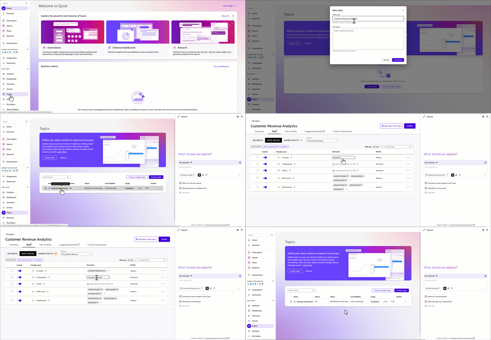
Figure 11: Create a Quick Topic
Create a Space for your team
Spaces bring together dashboards, topics, datasets, documents, and other resources into organized, collaborative workspaces. By centralizing related assets in a single workspace, Spaces reduce context-switching, accelerate onboarding, so everyone is working from the same trusted data sources.
What to include in your Quick Space
- Dashboard – Add the dashboard Market Segment Dashboard published from your
mv_customer_revenueanalysis. This gives team members instant access to visualizations such as revenue by market segment, top customers by order volume, and revenue distribution. - Topic – Connect the Customer Revenue Analytics (built on the
mv_customer_revenuematerialized view) to enable natural language queries directly against your Amazon Redshift data. - Optionally, you can upload supporting context to ground your team’s analysis:
- Data dictionary or field definitions for
mv_customer_revenue - Market segment definitions (AUTOMOBILE, BUILDING, FURNITURE, MACHINERY, HOUSEHOLD)
- Business rules for revenue calculation (for example, how discounts are applied in the TPC-H model)
- This implementation guide, so new team members can onboard quickly
- Data dictionary or field definitions for
To create the Quick Space
- From the left navigation menu, choose Spaces, then choose Create space.
- Enter a name, for example, Customer Revenue & Segmentation.
- Enter a description. For example:
Centralized workspace for customer revenue analysis powered by Amazon Redshift includes interactive dashboards, natural language query access to customer and segment data, and supports documentation for the TPC-H revenue model.
- Add knowledge by connecting the Market Segment Dashboard and topic Customer Revenue Analytics.
- You can invite team members, such as finance, sales operations, and segment owners, and set appropriate permissions.
Your Space is now ready for collaborative data exploration.
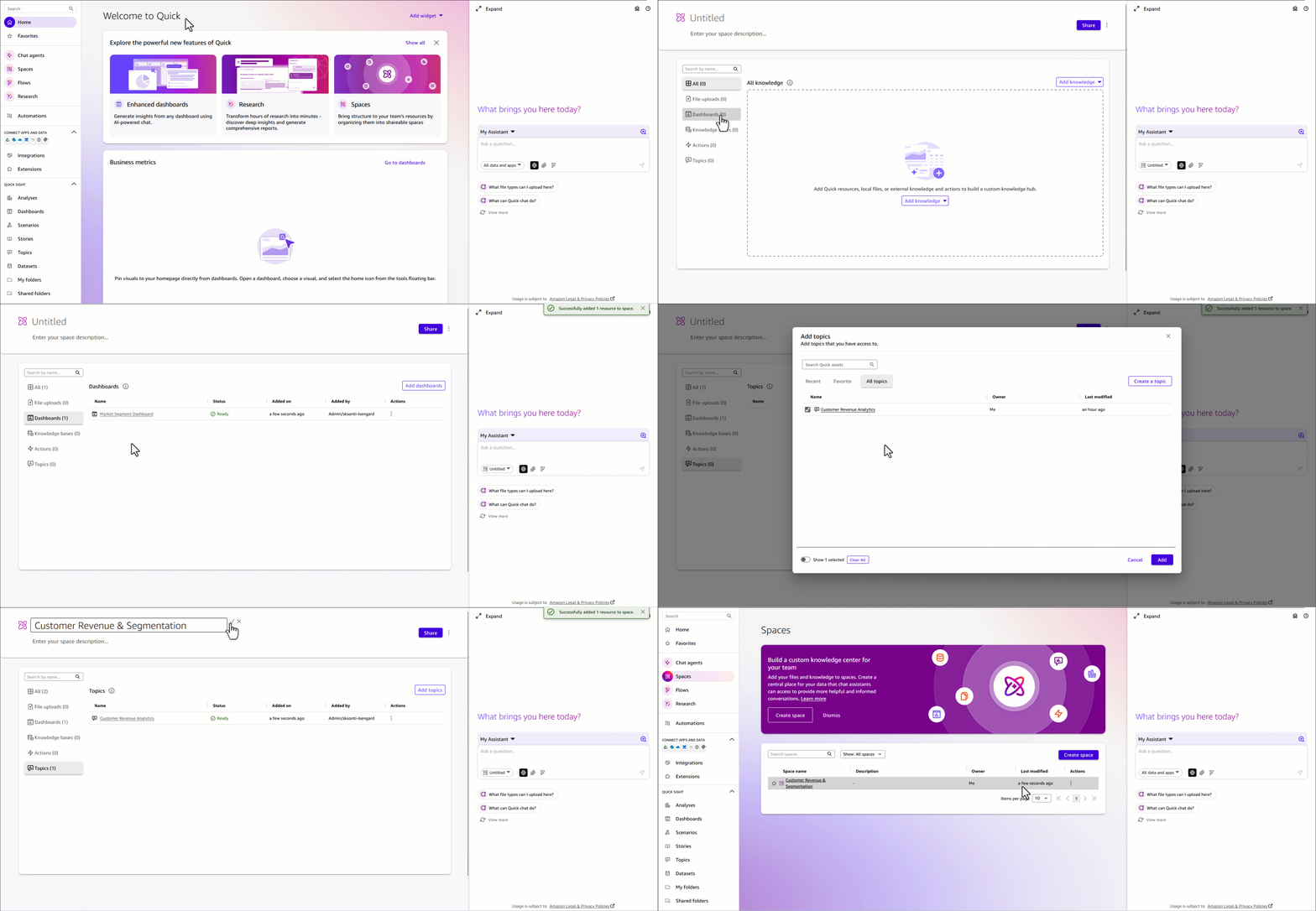
Figure 12: Create a Quick Space
Build chat agents
A custom chat agent delivers conversational AI experiences that understand business context and provide intelligent, grounded responses to user queries. These agents go beyond question-and-answer interactions. They synthesize knowledge from your dashboards, topics, datasets, and documents to explain trends, surface anomalies, guide users through complex analytics workflows, and recommend next steps.
Rather than requiring users to navigate multiple tools or write SQL queries, agents serve as a single conversational interface to your entire analytics environment. Agents can also connect to Actions, pre-built integrations with enterprise tools such as Slack, Microsoft Teams, Outlook, and SharePoint, enabling them to answer questions and trigger real-world workflows, send notifications, create tasks, and interact with external systems directly from the conversation. Custom agents can be tailored to specific business domains, teams, or use cases so that responses align with organizational terminology, data definitions, and business processes. After created, agents can be shared across teams, enabling consistent, actionable, AI-powered data access at scale. For teams working with the mv_customer_revenue dataset, we recommend creating a dedicated Customer Revenue Analysis Agent. This is a purpose-built conversational assistant grounded in your Amazon Redshift data, dashboards, and the Customer Revenue & Segmentation Space.
Create a Quick chat agent
There are two ways that you can use Amazon Quick to create a Quick agent. You can use the navigation menu or directly from Space. The following steps walk you through creating one from the navigation menu.
To create a Quick chat agent
- From the left navigation menu, choose Agents, then choose Create agent.
- Enter a name for your agent, for example, Customer Revenue Analyst.
- Enter a description. For example:
An AI assistant for analyzing customer revenue, market segment performance, and order trends using our Amazon Redshift or data warehouse.
- Under Knowledge Sources, add the Customer Revenue & Segmentation Space as a data source. This gives your agent access to the dashboards, topics, and reference documents you’ve already built.
- (Optional) Define custom persona instructions to align the agent’s responses with your business context. For example, specifying preferred terminology, response style, or the types of questions it should prioritize.
- Choose Launch chat agent.
- Start having a conversation with your data. You are welcome to ask any questions. The following are some examples.
- Which market segment generated most revenue?
- Show me order trends
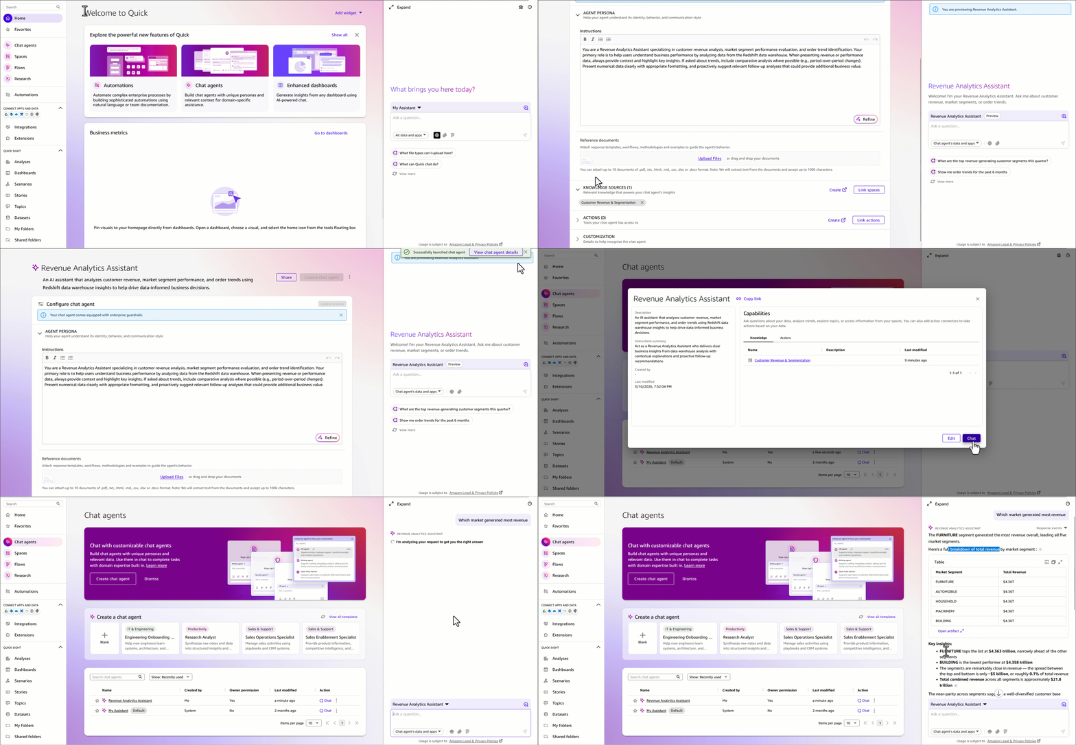
Figure 13: Create a Quick Chat agent
To share your Quick chat agent
After your agent is published, choose Share and invite team members or share it across your organization. Custom agents can be tailored to specific business contexts so that different teams can get AI assistance that speaks their language, without needing to configure anything themselves.
Create Quick Flows
Quick Flows automate repetitive tasks and orchestrate multi-step workflows across your entire analytics environment. This removes manual effort, reducing human error, and ensuring consistent execution of critical business processes. Flows can be triggered on a schedule or launched on demand, giving you flexible control over when and how automation runs.
You can build flows that span the full analytics lifecycle: monitoring data quality and flagging anomalies, generating and distributing scheduled reports to stakeholders, and triggering downstream actions in integrated systems such as Slack, Outlook. Amazon Quick gives you three ways to create a flow, so whether you prefer a no-code conversation or a visual step-by-step builder, there’s an option that fits how you work.
To create a flow from chat
- While conversing with My Assistant or a custom agent, describe the workflow that you want to automate in plain English.
- Amazon Quick generates the flow and offers to create it directly from your conversation — no configuration screens required.
To create a flow from a natural language description
- From the left navigation menu, choose Flows, then choose Create flow.
- Enter a plain-English description of your workflow. For example:
” Query revenue data by market segments. Filter by order count and all dates. Search web for comparable relevant market trends. Generate formatted summary reports providing market summary and look ahead per segment. ”
- Amazon Quick automatically generates the complete workflow with all the necessary steps.
- Optionally, you can add additional steps.
- Choose Run Mode to test the Flow.
- After your flow is created, share it with team members or publish it to your organization’s flow library, so everyone benefits from the same automation without having to rebuild it independently.
Figure 14: Create a Quick Flow to generate summaries and publish dashboards
For more complex flow, review weekly customer revenue summary flow as an example.
- Queries the
mv_customer_revenuematerialized view in Amazon Redshift for the latest weekly revenue figures by market segment. - Compares results against the prior week to calculate segment-level variance.
- Generates a formatted summary report and publishes it to the Customer Revenue & Segmentation Space.
- Sends a notification through email or Slack to finance, sales operations, and segment owners with a direct link to the updated dashboard.
- Flags any segment where revenue has declined more than a defined threshold, routing an alert to the appropriate owner for follow-up.
This flow transforms what might otherwise be a manual, multi-step reporting process into a fully automated pipeline, so stakeholders receive consistent, timely revenue insights without analyst intervention and saving analysts an estimated 3–5 hours per week. For detailed guidance on creating and managing flows, see Using Amazon Quick Flows. Also review Create workflows for routine tasks demo.
Cleanup
Consider deleting the following resources created while following this post to avoid incurring costs. We encourage you to use the trials at no cost as much as possible to familiarize yourself with the features described.
- Delete the Amazon Redshift Serverless workgroup and namespace.
- Delete Athena workgroup and S3 Buckets.
- Delete the Amazon Quick account used while following this post. If you used an existing account, delete the data sets, dashboards, topics, spaces, agents and flows created.
Conclusion
This integrated approach to business intelligence combines the power of AWS SQL analytics engines with Amazon Quick generative AI capabilities to deliver comprehensive analytics solutions. By following these implementation steps, you establish a foundation for traditional BI reporting, interactive dashboards, natural language data exploration, and intelligent workflow automation. The architecture scales from proof-of-concept implementations to production deployments, transforming how organizations access and act on data insights. For more information about Amazon Quick features and capabilities, see the Amazon Quick documentation. To learn more about Amazon Redshift, visit the Amazon Redshift product page. For Amazon Athena details, see the Amazon Athena product page.
About the authors
MSI XpertStation WS300 NVIDIA GB300 Station and More at the MSI NVIDIA GTC 2026 Booth
Post Syndicated from Patrick Kennedy original https://www.servethehome.com/msi-xpertstation-ws300-nvidia-gb300-station-and-more-at-the-msi-nvidia-gtc-2026-booth/
At NVIDIA GTCX 2026, we saw MSI servers ranging from the desktop EdgeXpert and XpertStation WS300 to air and liquid-cooled multi-GPU servers
The post MSI XpertStation WS300 NVIDIA GB300 Station and More at the MSI NVIDIA GTC 2026 Booth appeared first on ServeTheHome.
AWS Weekly Roundup: AWS DevOps Agent & Security Agent GA, Product Lifecycle updates, and more (April 6, 2026)
Post Syndicated from Channy Yun (윤석찬) original https://aws.amazon.com/blogs/aws/aws-weekly-roundup-aws-devops-agent-security-agent-ga-product-lifecycle-updates-and-more-april-6-2026/
Last week, I visited AWS Hong Kong User Group with my team. Hong Kong has a small but strong community, and their energy and passion are high. They recently started a new AI user group, and we hope more people will join. I was able to strengthen my bond with the community through great food and conversation.
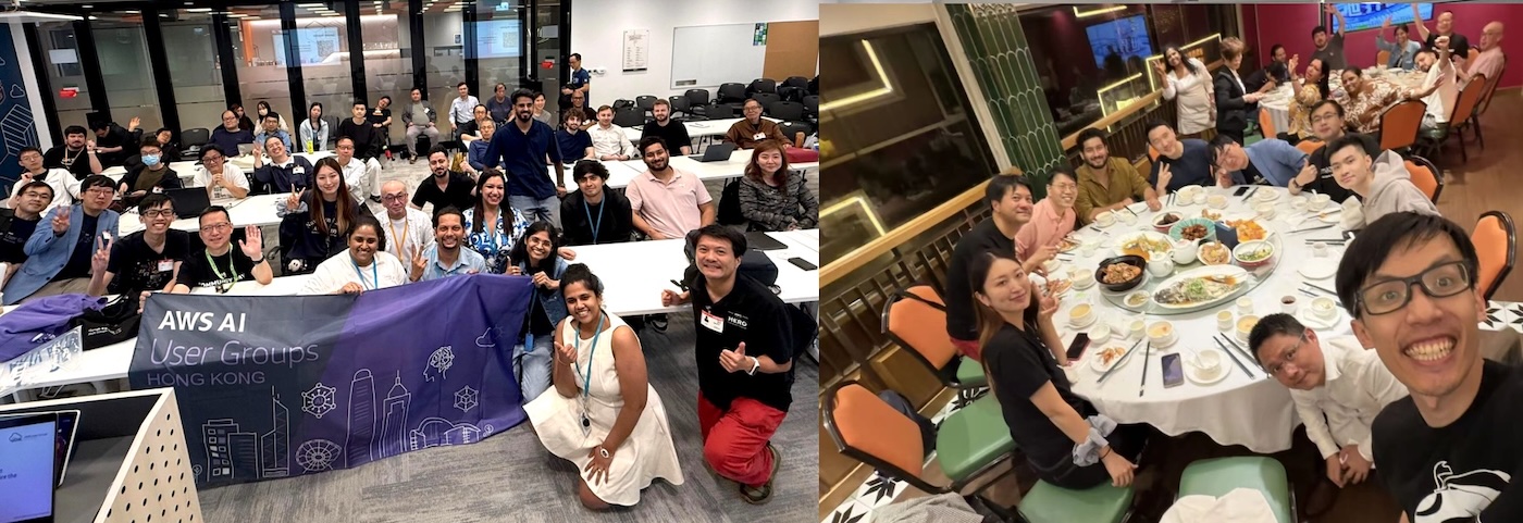
This week, I”ll first take a closer look at some of the key launches.
AWS DevOps Agent and Security Agent GA
 At the last re:Invent, we introduced the concept of frontier agents that work autonomously across multiple steps to achieve outcomes, operating continuously until the job is done. The first two—AWS DevOps Agent and AWS Security Agent—are now generally available after the preview.
AWS DevOps Agent helps you run cloud operations—investigating incidents, reducing time to resolution, and preventing issues before they happen. Customers like United Airlines, Western Governors University, and T-Mobile are already using DevOps Agent to accelerate incident response and simplify operations at scale. At WGU, resolution time dropped from hours to minutes, and in preview customers report up to 75% lower MTTR and 3 to 5 times faster resolution. Learn more in Sébastien’s preview blog post and GA announcement.
AWS Security Agent brings continuous, context-aware penetration testing into the development lifecycle. This agent operates like a human penetration tester. Customers including LG CNS, HENNGE, and Wayspring are seeing strong results. At LG CNS, teams estimate over 50% faster testing and ~30% lower costs, along with significantly fewer false positives. Learn more in Esra’s preview blog post and GA announcement.
Both are designed to work across AWS cloud, multicloud, and on-prem environments. You can have an always-available teammate that can handle the heavy lifting, so you can focus on what matters most.
AWS Service Availability Updates
When the availability of an AWS service or feature changes, we provide customers guidance in AWS Product Lifecycle Changes on available alternatives and support for migration so that disruptions to your operations are minimized. The following lifecycle changes were updated on March 31, 2026.
- Availability change guide for services in maintenance
- AWS App Runner
- AWS Audit Manager
- AWS CloudTrail – Lake
- AWS Glue – Ray jobs
- AWS IoT FleetWise
- Amazon Application Recovery Controller (ARC) – Readiness Check
- Amazon Comprehend – Topic Modeling, Event Detection, and Prompt Safety Classification
- Amazon Rekognition – Streaming Events and Batch Image Content Moderation
- Amazon Simple Notification Service (Amazon SNS) – Message Data Protection (MDP)
- Availability change guide for services in sunset:
- Services reaching in sunset:
- Amazon Chime SDK – Proxy Sessions
We understand that changes in availability can impact your operations. For specific guidance, consult the relevant service documentation or contact AWS Support.
Last week’s launches
Here are last week’s launches that caught my attention:
- Amazon ECS announces Managed Daemons for ECS Managed Instances
- New AWS Sustainability console: Scope 1–3 reporting in one place
- Amazon Bedrock AgentCore Evaluations is now generally available
- AWS Transform custom announces general availability of automated codebase analysis
- Amazon CloudWatch launches OpenTelemetry Container Insights for Amazon EKS (Preview)
- New compute-optimized instance bundles for Amazon Lightsail with up to 72 vCPUs
- Amazon CloudFront now supports SHA-256 for signed URLs and signed cookies
For a full list of AWS announcements, be sure to keep an eye on the What’s New with AWS page.
Additional updates
Here are some additional news items that you might find interesting:
- Architecting for agentic AI development on AWS
- Optimizing data transfer costs when using AWS Network Load Balancer
- Announcing AWS World Sports Innovation Cup – Will your idea change the game?
- 5 Techniques to Stop AI agent hallucinations in production
- Explore the global AWS Community through a 3D interactive globe
For a full list of AWS blog posts, be sure to keep an eye on the AWS Blogs page.
Learn more about AWS, browse and join upcoming AWS led in-person and virtual events, startup events, and developer-focused events as well as AWS Summits and AWS Community Days. Join the AWS Builder Center to connect with builders, share solutions, and access content that supports your development.
That’s all for this week. Check back next Monday for another Weekly Roundup!
— Channy
[$] Protecting against TPM interposer attacks
Post Syndicated from jake original https://lwn.net/Articles/1064685/
The Trusted
Platform Module (TPM) is a widely misunderstood piece of hardware (or
firmware) that lives in most x86-based computers. At SCALE 23x in Pasadena, California,
James Bottomley gave a presentation on the TPM and the work that he and
others have done to enable the Linux kernel to work with it. In
particular, he described the problems with interposer attacks, which target
the communication between the TPM and the kernel, and what has
been added to the kernel to thwart them.
6.6.133 stable kernel released
Post Syndicated from jzb original https://lwn.net/Articles/1066507/
Greg Kroah-Hartman has released the 6.6.133 stable kernel. This reverts
a backporting mistake that removed file descriptor checks which
led to kernel panics if the fgetxattr, flistxattr,
fremovexattr, or fsetxattr functions were called
from user space with a file descriptor that did not reference an open
file.
Ruthie Rogers on the Value of Restaurants
Post Syndicated from The Atlantic original https://www.youtube.com/shorts/F6VPAKOXsYU
Security updates for Monday
Post Syndicated from jzb original https://lwn.net/Articles/1066505/
Security updates have been issued by AlmaLinux (freerdp, grafana, grafana-pcp, gstreamer1-plugins-bad-free, gstreamer1-plugins-base, gstreamer1-plugins-good, and gstreamer1-plugins-ugly-free, kernel, libpng12, libpng15, perl-YAML-Syck, python3, and rsync), Debian (dovecot, libxml-parser-perl, pyasn1, python-tornado, roundcube, tor, trafficserver, and valkey), Fedora (bind9-next, chromium, cmake, domoticz, freerdp, giflib, gst-devtools, gst-editing-services, gstreamer1, gstreamer1-doc, gstreamer1-plugin-libav, gstreamer1-plugins-bad-free, gstreamer1-plugins-base, gstreamer1-plugins-good, gstreamer1-plugins-ugly-free, gstreamer1-rtsp-server, gstreamer1-vaapi, libgsasl, libinput, libopenmpt, mapserver, mingw-binutils, mingw-gstreamer1, mingw-gstreamer1-plugins-bad-free, mingw-gstreamer1-plugins-base, mingw-gstreamer1-plugins-good, mingw-libpng, mingw-python3, nginx-mod-modsecurity, openbao, python-gstreamer1, python3.12, python3.13, python3.14, python3.9, rust, rust-sccache, tcpflow, and vim), Red Hat (ncurses), Slackware (infozip and krita), SUSE (chromium, corosync, keybase-client, libinput-devel, osslsigncode, python-pillow, python311-Flask-Cors, python313, and python314), and Ubuntu (libarchive and spip).
Why NATO?
Post Syndicated from The History Guy: History Deserves to Be Remembered original https://www.youtube.com/watch?v=62d7ZmxMhiY