Post Syndicated from The Atlantic original https://www.youtube.com/watch?v=wS6GNorQGMU
The Atlantic Presents: The 2026 Michael Kelly Award
Post Syndicated from The Atlantic original https://www.youtube.com/watch?v=n23E7V-Dgx8
Friday Squid Blogging: On Squid Egg Sacs
Post Syndicated from Bruce Schneier original https://www.schneier.com/blog/archives/2026/09/friday-squid-blogging-on-squid-egg-sacs.html
Short essay about squid egg sacs.
As usual, you can also use this squid post to talk about the security stories in the news that I haven’t covered.
Pete Buttigieg: Amending the Constitution Should Not Be Beyond Ambition
Post Syndicated from The Atlantic original https://www.youtube.com/shorts/KSx7N_RVDic
Conversations With Shenna Bellows and Brad Raffensperger
Post Syndicated from The Atlantic original https://www.youtube.com/watch?v=qNo_dIFPnpg
The Tech Economy: Is AI Reshaping America?
Post Syndicated from The Atlantic original https://www.youtube.com/watch?v=F_lINL20h3c
Why Ethics Is About More Than Just Helping Other People
Post Syndicated from The Atlantic original https://www.youtube.com/shorts/_kuz6-FP8BY
NYT Executive Editor Joe Kahn Says Quality, Original Reporting ‘Won’t Be Suppressed’
Post Syndicated from The Atlantic original https://www.youtube.com/shorts/rIc4-mCGC8E
Saving another 100TB of RAM with math (and Rust)
Post Syndicated from Kevin Guthrie original https://blog.cloudflare.com/saving-100-tb-of-ram-with-math/
Cloudflare operates at a scale so big that even after working here for years, it doesn’t seem real. We have thousands of servers all over the world with petabytes of RAM and millions of CPU cores, and all of it is pushed to the max. As vast as those resources feel, they are still finite, and when you need every service to run on every node, it doesn’t leave room for wasted space.
At this scale, small improvements are greatly magnified, so even 1%-at-a-time improvements are worth celebrating. And some tweaks add up to a lot more: in this post, we’ll look at how small changes to a single algorithm reduced the memory footprint of one of our Pingora-based services significantly. That allowed us to reclaim more than 100TB of RAM globally, on top of the 100TB of memory the DNS team was able to shed last month.
Waste not
Maintaining equitable resource sharing between teams is not easy, especially in large organizations. One of the ways Cloudflare ensures the balance is kept is through the tireless efforts of the wonderful Performance team.
This story starts with a ticket filed by Ivan who found: Excessive memory usage from pingora-ketama in Pingora Backend Router. The finding was that our internal load-balancing service, Pingora Backend Router (yes, PBR), was using significantly more memory than expected — specifically in structures associated with pingora-ketama, which is our open-source library for handling consistent hashing.
In order to talk about how we addressed this seeming overuse of memory, we need to talk about what consistent hashing even is, why we are using it in PBR, and how it became so memory hungry. Along the way, we’ll learn some Rust and even a little math.
Consistent hashing
Consistent hashing is a widely used method for distributing tasks across multiple servers in a way that does not require large changes when servers are added or removed. Internally we use it to route cacheable requests to servers by URL. This allows us to keep only one copy of a file stored per data center and gives a stable way to find the location of each file. We have mentioned this system before, but let’s take the time to walk through how and why this algorithm is used and how it works.
The key concept of consistent hashing is that while hash functions can accept any kind of input, their output is limited to a single unsigned integer (32, 64, or 128-bit integers depending on which hash function). This allows us to relate tasks and servers to each other in a consistent way. Most discussions of consistent hashing have you think of that output space as a continuous, circular ring that wraps around from its max value to zero. This depiction makes for some nice visualizations, but it can also make the simple concept of integer ranges seem more complicated than it needs to be. For our discussion, we’ll represent the 32-bit output of our hash function as a number line.
Now, let’s say we have a set of servers, A, B, & C, and a set of tasks t-z. We can map each onto the number line based on the hash of their representative values, so something like IP addresses for servers and cache keys for tasks.
Assigning tasks to servers is now just a matter of finding the first server to the left of each task. We can represent this visually by coloring in the region of hashes that will be associated with each server. Notice that the range covered by server C wraps around to the beginning, hence the idea that hashes exist in a ring.
And that’s it. At a base level, consistent hashing is this simple — but it doesn’t take long to see that there is room for improvement. Notice that the range covered by server A in our example is significantly larger than that of either B or C. This is a problem because the fraction of the requests a server handles is going to be proportional to the size of its range on the number line. Ideally we would like to guarantee each server will have an equal size, but because hashes are essentially random numbers, we have to talk about the size of the regions in terms of statistics. 😨
Math and consequences
First: don’t panic. I promise I'm not about to lie to you and that we will stay safely within the bounds of a day-one probability lesson. When we talk about statistical distributions, there are two big factors that help us quantify uncertainty in helpful ways: expected value and standard deviation. In (over-)simplified terms, expected value gives us a point where measurements based on a distribution will be centered, and standard deviation tells how close to that central point most measurements are likely to be.
For consistent hashing, we can calculate these factors for the fractional size of the range associated with one of N servers. (Details on where this formula comes from later).
In terms of concrete numbers, let’s say we have 100 servers. The formulas above give:
That tells us that we can expect that the range each server handles will be centered around 0.99% of the total and most of the lengths to fall within 1% of what's expected. This sounds good until we realize that that’s 0.99% of the total length. We need to scale the standard deviation by the expected value to see how big the error is as a fraction of the target size. This value is called the coefficient of variation.
What if we add hashes?
The simplicity of consistent hashing is a double-edged sword. It’s easy to understand and implement because everything is turned into easily-relatable hashes on the same numberline, but any improvements to the system will also need to be relatable to that numberline. That means the solution to any consistent hashing problem can only be more hashes. It’s less like a golden hammer (a tool with which all problems look like nails) and more like a golden nail in that it turns all tools into hammers.
To solve the problem of imbalanced workloads, we can add multiple hashes to represent each server instead of just one. We’ll get to the math behind this momentarily, but it should make some intuitive sense that while each individual range has a large standard deviation, adding a bunch together should make their total size even out. If we take our three-server example from the above diagrams and add two more hashes at random for each server, we see that it helps even out each server’s workload.
This is an admittedly contrived example. The random nature of the system means there’s no guarantee how much improvement you will get from adding 2 additional hashes per server, but it should make some intuitive sense that combining more of these hash segments together produces a more even distribution. Each segment in the sum has a chance of balancing another. Maybe one is too short; maybe one is too long. This is essentially what the law of large numbers tells us should happen… The obvious problem is it only works for large numbers. In NGINX, the baseline number of hashes per server is hardcoded to 160, and Pingora uses the same value as the default. I’ll spare you the math for now, but if we go back to our 100-server example, if we use 160 points per server instead of just one, the coefficient of variation (which we can think of like an error margin) drops from about 99% to about 8%, a significant improvement.
What if we add more hashes?
We saw above that increasing the number of hashes per server by a constant amount allows us to improve how evenly workloads are distributed per server, but what if we don’t want to distribute the work evenly? In Cloudflare’s case, we have some servers that have more storage space than others, so it would be better to have the number of requests allotted to a server be proportional to its disk space. One way to accomplish this is with the ketama algorithm. The naming is a little funny because the algorithm is named after the library where it was first implemented, and the library was named … well you can google it 😶🌫️.
For us, since we want workload to be scaled based on storage, we can use the disk space as the weight, which is exactly what the Pingora team has been doing for years. Elsewhere in the company where workloads are more compute-intensive, weights might be based on CPU or GPU count.
What if we add even more hashes???
The last problem we need to address is that so far we are working under the assumption that any server can handle any request, but in practice that is not the case. Things like compliance requirements or enabled caching features mean only a subset of servers can handle any particular request. Unfortunately, unlike before, we can’t solve this problem by adding more hashes to the same ring. We have to add completely new rings, and not only that — every combination of features potentially needs its own specific ring!
Storage improvements
One big improvement came from Zaidoon, who had an insight about our struct for storing hashes in PBR. That struct looks like this:
Unfortunately, Rust doesn’t make it that easy. Changing the size of the index as we did above does nothing to reduce the memory footprint. This is because Rust has alignment rules that require the size of a structure in memory to be a multiple of its largest (or “most aligned”) field. In this case, the hash is the largest with four bytes, so when stored in memory, a Point is required to have size $mN \times 4m$, so the minimum size is eight bytes.
Luckily there are well-known ways around this. You (meaning me) might be tempted to use #[repr(packed)], but that is controversial for good reasons. A safer but less readable solution is to store the hash and index as raw byte array and access them with getters. Both methods compile to the same thing.
This simple (if wordy) change reduces the amount of memory used for consistent hashing by a whopping 25%! In order to do better than that, we’ll need to jump back into the math, so everybody hang on to something; this is the home stretch.
What if we tried fewer hashes?
You may have noticed that we gave the formula for the standard deviation for the case where there is only one hash per server. Deriving the formula for the case where there are $m k m$ hashes per server is not easy, and most sources only give you an approximation or an asymptotic limit, but not us. I might not be a statistician, but I grew up with a calculus teacher (Hi, Mom!), and I wanted to know the actual value. The full derivation is in a supplemental post, but here is the payoff.
To see how increasing the hash count improves the accuracy, we need to look again at the coefficient of variation.
The predictions from my beautiful math only work if we think about hashes in a continuous ring, but in practice we use 32-bit numbers for the hashes that have the potential for collisions, and the probability of collisions goes up surprisingly quickly as the number of hashes increases (see the birthday paradox). Collisions matter because in the ideal case, every hash contributes to the volume and distribution of requests handled by the associated server, but a collision means some contributions are randomly dropped, introducing unpredictable error. If we compare some simulated results with 32-bit hashes with the predicted error rate, we can see that for data centers with 2048 servers, the error rate increases: between 10,000 and 100,000 hashes per server.
Ultimately, even though this realization feels kind of bad, it’s great news for our plan to reclaim some RAM! Now that we have some math to back it up, we determined that we could decrease the number of hashes we were generating for each server by 90% without incurring any appreciable error, so that is what we set out to do.
Migrating without melting origins
There was one more problem: changing the hash ring changes where some cacheable requests go. Even if the new ring is better, switching the whole network at once would effectively invalidate almost all cached content. It would turn a memory optimization into an apocalyptic increase in origin traffic.
So we did not make this a single global flip. For a while, PBR carried both versions of the cacheable load balancer in memory: the old ketama ring and the new smaller one. Each request used our normal migration framework to decide which ring should select the backend. That meant the rollout decision was stable per request hash, and it also gave us a clean rollback path. If anything looked wrong, we could send new requests back through the old ring without redeploying PBR.
We then rolled the migration out in layers. We started with small validation locations, moved through progressively larger groups of data centers, and only then continued toward the rest of the world.
The important part was that we controlled two dimensions independently: how much traffic used the new ring, and where that traffic was allowed to move. A plain global percentage rollout would have spread cache churn everywhere at once. Data-center-scoped rollout kept the blast radius small and made it much easier to tell whether a change was actually safe.
During the migration, we watched backend-selection traces, ring-version counters, PBR connection errors, process memory, startup time, cache behavior, and origin traffic. Once the migration reached 100%, we removed the temporary old-ring path, and voila!
The chart above shows the comparison of the memory used by PBR the week of the change compared with data from a few weeks before, as well as the result of subtracting one from the other. The sharp drop is the day where the version of PBR with the large (now unused) hash rings was decommissioned forever. Looking at the difference, we get the satisfying result that our changes dropped the used memory by 100TB!
Try it yourself
All the changes we talked about in this post are available now in the pingora-ketama crate in the form of a (for now) unadvertised cargo feature. The v2 ring has the compacted storage format, a faster sorting method, and the ability to scale the base number of hashes per node. Our focus in making these changes had to be on stability and control, so the v1 ring is identical to what pingora ketama has always used, and the library makes it possible to run both simultaneously and decide on a request-by-request basis which to use and when.
Beyond trying our literal consistent hashing changes, I would like you to take away from this some inspiration to dig into your own systems to see what “simple” or “obvious” decisions are hiding potential wins, if you’re willing to get into the numbers. You might not be able to solve all your problems with Rust, but math is universal.
Дубайбад – бившото Аудиовидео Орфей в Изгрев
Post Syndicated from Боян Юруков original https://yurukov.net/blog/2026/dubaibad2/

Днес излезе заявление за издаване на ПУП на имот от 26 декара в кв. Изгрев на бившото Аудиовидео Орфей. Писах преди, че заради бездействие на министерството на културата и липса на отношение от районната администрация държавата загуби имота.
През май дадох пример в картата на застрояването как би изглеждала сградата, ако се използват максимално позволените параметри. Скицата към заявлението от днес показва много по-лоши планове. Както винаги казвам откакто се вгледах в застрояването – ако се питате дали ще се застрои, то отговорът е да и ще е по-зле отколкото си представяте. Не просто надвишават разрешените параметри и практически няма място за озеленяване, но и ще блокират улиците в района.
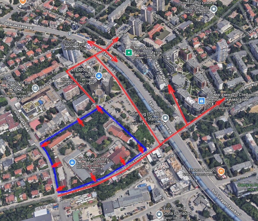
Около имота има само малки квартални улици направени за няколко десетки семейства живеещи в двуетажни къщи. В случая говорим за стотици отгоре на това. Първият изход е по ул. Самоков в посока кръговото на 4-ти км. Преди това се превръща в ул. Тинтява и това кръстовище вече е изцяло блокирано сутрин и вечер. Другият път е към метроспирката на Кюри. Кръстовището там е по-малко блокирано, но не е направено за такъв трафик, нито малките квартални улици, през които ще минават стотици коли в повече всеки ден.
Нямам съмнения, че ще си купят обаче транспортен анализ с удобните изводи. Видяхме го при няколко строежа в близост. Тези не са публични все още макар да целят защита на обществените интереси и безопасност. За абсурдните твърдения в тях научаваме единствено от дискусиите в комисия на НАГ.

Имотът е 26195, с кинт. 3.5 и максимална височина 75 метра. Дори предполагайки щедри като височина фоайета и големи студия, каквито се предвиждат в сделката с Аудиовидео Орфей, пак скицата ни показва разгърната площ от 30% повече от разрешеното по устройствен план. Единственият начин това да стане е да си купят гласове от ГЕРБ, БСП и ВМРО в СОС, които да им го позволят. Височината също се надвишава на едно място и предвижда почти 80 м.
Озеленяването трябва да е 40%, от които една четвърт да са високи дървета. Скицата показва 50% застроена площ. Като включим тротоари, алеи, входове на гаражи, трансформатори и друга инфраструктура, трудно може да се види как биха постигнали 40% озеленяване на така представената скица. Отчитайки отстоянията между сградите, практически е невъзможно да поместят и 210 дървета, какъвто е минимума, които да оцелеят и да имат задължителните по наредба отстояния от сгради и бордюри. От месеци има сигнали, че сегашните дървета се изсичат незаконно. Районната община мълчи въпреки сигналите. Няма разрешение за строеж и основание да им го разрешат, а те и не публикуват такива разрешения, макар да са длъжни по наредба. Бързат да секат обаче, защото биха били пречка за бъдещото разрешение за строеж.
А ще е пречка, защото според същата скица ще бетонират и запечатат изцяло 26-те декара за изграждането на 2 етажа подземен гараж. Това, както и масовата практика в (не)озеленяването в София, за която дадох примери. Единият беше за готови сгради, а другият – за строящи се съвсем наблизо. Отново, не очаквам да е проблем дори да не боднат едно дръвче и пак да вземат акт 16. Сега водя две дела с ДНСК, които отказват да предоставят административен документ показващ кой е подписал, че всичко е наред с озеленяването на две готови сгради с ясно видими нарушения. Не очаквам нещо различно тук.
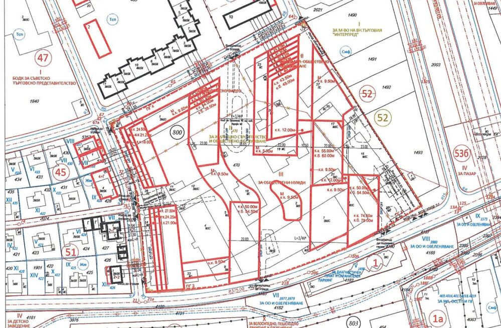
Проектът е още на етап заявление за ПУП. Не е прието или одобрено. Въведох го в сегашния му вид на картата на застрояването, защото това е планът на инвеститора. С други думи, общината нищо не е разрешила. Научаваме за ПУП-а заради прозрачност, която Терзиев въведе в началото на миналата година, точно, за да знаем за подобни планове и да реагираме, защото именно този етап е критичен и до сега оставаше скрит.
Тепърва ще минава комисия, ще се иска становище от районната община и експерти. Районният кмет отговаря на такива проекти винаги без забележки и съгласие до сега като пример е проекта на Тинтява 80, сега започвания в съседство и вече с проблеми строеж на бившите сервизи бензиностанция Петрол, както и кулите на мястото на сградата на ПИБ. Та не очаквам много от там. Надеждата ми е, че комисията в НАГ ще изиска значително намаление на измеренията на проекта с оглед на инфраструктурата и цялостното планиране на квартала. Ще следим обсъжданията, но именно на нито ПУП е важно какво се реши, а не да се действа както в миналото на парче.
Leave the Class Path in the Rearview Mirror
Post Syndicated from Netflix Technology Blog original https://netflixtechblog.com/leave-the-class-path-in-the-rearview-mirror-67a85b15b6be
Introducing composable, module system native and agent friendly command line tools for modern Java development
By Danny Thomas, JVM Ecosystem Team

Recent work on the Java language to pave the on-ramp has made it easier than ever to start a Java program and evolve it using the full language and platform. At the end of that on-ramp lies Java’s mature build and dependency management ecosystem, capable of carrying software to enormous scale and complexity.
That ecosystem reached its maturity by developing strong models for projects, dependencies, and builds. When the Java Module System arrived, those models were already serving developers exceptionally well. The module descriptor consequently became just another description of the project to keep in agreement.
We’re excited to announce a preview of ja and its family of composable tools, that build on the capabilities of the Java Module System to provide a modern command line development experience for Java. We take the module descriptor and make it a complete description of a project, with dependency versions sitting naturally beside its requires directives and module metadata provided through documentation tags:
/**
 * @mainClass com.example.application.Main
 */
module com.example.application {
    requires com.example.framework; // @1.2.3
}
Combined with command line ergonomics you’re used to in other languages, creating and consuming Java modules has never been easier.
Composable Tools
Java developers have long been exceptionally well served by graphical tools. An IDE formats source, navigates between declarations and usages, presents API documentation, and maintains a compiled view of the project. That experience has been so complete that Java has had less need to expose the same capabilities through small, composable command line tools. Those gaps become quickly apparent when coding agents work with the Java language, with agents frequently struggling to locate dependencies, documentation and sources.
ja only provides command line ergonomics and tool orchestration, each feature is underpinned by a standalone tool. You don’t need to adopt ja to get the benefit of these tools, you can compose them in any way you choose:
- jig performs module version resolution, compilation and assembly, outputting standard module system arguments for use with other tools. It is also the bridge to and from Maven repositories providing a standalone module proxy and publishing commands
- jfmt formats source using the Code Conventions for the Java Programming Language, adapted for the modern Java language. Avoids the very common whitespace, indentation, import ordering and qualified class references introduced in agent written code
- jist provides source aware symbol search, providing a grep style interface for understanding class files and their associated sources. Gives coding agents access to symbols and sources without indexing, LSPs or MCPs while interoperating with other build tools via an argument file contract
- jdocserver serves locally browsable API documentation
These projects use the tool discovery and execution capabilities of the platform, and are intended to be installed in your JDK along with the standard tools. They all implement Tool or ToolProvider, allowing them to be run in process.
This is also the tool discovery and execution model for ja. There we use OptionChecker and optional custom metadata to discover which module system options are supported so it can resolve the arguments on behalf of the tool. This provides a seamless transition from your source path modules to the standard JDK tooling such as jdeps, jlink and jshell.
Maven as a foundation
In a recent survey of the 1,000 most popular artifacts on Maven Central, just 232 had explicit module definitions and another 248 declared automatic module names. The remaining 520 expressed no Java module name opinion. The module system also makes no distinction between namespace and module name, so module-first tooling requires a solution to module naming and location in existing repositories.
Fortunately, Maven Central already gives published artifacts a verified namespace. Publishers prove control of reverse domain group IDs, reflecting Sonatype’s long standing case for namespaces in public repositories.
We use these conventions to establish a canonical Maven module coordinate, paring a verifiable DNS namespace with the complete module name, for example pkg:maven/com.netflix/com.netflix.tools.ja. For existing modules, authors choose to publish a single Maven relocation pom at the canonical coordinate, to allow for discovery of the original coordinate.
When neither are available, candidates are walked from the root of the namespace using common Maven artifact conventions inferring coordinates from module names. We also bundle a short list of aliases for the most popular modules that don’t use a reverse DNS module name, but we suggest authors should always namespace their modules. The module proxy in jig presents resolved modules using the filename based conventions for module naming, making even automatic modules without stable names safe when used with these tools.
These conventions and location strategies allow the majority of existing artifacts to be discovered using only the module name and version.
Integrity by default
ALL-UNNAMED has become unfortunately common in Java access options, because of the heavy use of the class path. It hides the source of the technical debt that applications are incurring by allowing such access and becomes increasingly consequential as Java moves toward Integrity by Default. For example, Preparing to Make Final Mean Final asks applications to explicitly authorize the modules allowed to mutate final fields.
We allow runtime access requirements to bedeclared as module metadata and carried with the module descriptor throughout the module’s lifecycle. For example a library may record the access it requires:
/**
* @enableFinalFieldMutation com.example.framework
*/
module com.example.framework {
}
However, the consuming application remains in control and must explicitly authorize the framework, for it to be available at runtime:
/**
* @mainClass com.example.application.Main
* @enableFinalFieldMutation com.example.framework
*/
module com.example.application {
    requires com.example.framework; // @1.2.3
}
The command line interface for ja allows the dependency and authorization to be added together:
ja require [email protected] \
 --enable-final-field-mutation com.example.framework
Without that authorization, dependency resolution fails with an unsatisfied access requirement. Native access follows the same model through @enableNativeAccess and qualified exports and opens are also supported.
Module integrity is ensured by persistent hashes of resolved binary dependencies in a module-info.hash file, sequent resolution verifies those hashes and rejects an artifact that has changed.
We also take a step further than the recent improvements to annotation processor security by treating annotation processing as an explicit code generation step. The resulting sources are alongside regular module source, making them visible in code review and allowing a module to be assembled without executing generator code.
Make modules your default
We think every Java project should be modular, regardless of the build tool you’re using. If you’re a library author producing automatic modules, we’d encourage you to avoid split packages and produce explicit modules.
You can get started with our tools today with our installation guide.

Leave the Class Path in the Rearview Mirror was originally published in Netflix TechBlog on Medium, where people are continuing the conversation by highlighting and responding to this story.
Conversations With Jeffrey Goldberg, Amna Nawaz, Joe Kahn, and More
Post Syndicated from The Atlantic original https://www.youtube.com/watch?v=thu0d15jvlY
Running self-hosted AI agent sandboxes with AWS Lambda MicroVMs
Post Syndicated from Brian Krygsman original https://aws.amazon.com/blogs/compute/running-self-hosted-ai-agent-sandboxes-with-aws-lambda-microvms/
Organizations are building AI agents that autonomously write code, query databases, and interact with internal systems on behalf of their teams. These agents handle use cases such as automated code review, data pipeline optimization, and infrastructure troubleshooting. When your AI agent generates a shell command, queries a database, or writes to a file system, that code needs a secure environment to run in. Without isolation, one session’s tool calls can contaminate another session’s state, inadvertently expose sensitive data across tenants, or unintentionally allow untrusted code to reach production resources. Self-hosted sandboxes solve this by keeping agent execution within your own AWS account, giving you full control over networking, secrets, and governance.
Say you’re building an internal AI agent that optimizes database queries for your engineering team. A developer asks it to find the ten slowest queries in your analytics database, rewrite them with better indexing, and test the results. That’s three tool calls in a single session. One hits a live database with real credentials. One generates code. One executes it. Now multiply that by fifty developers using the assistant at the same time. Each session needs its own credentials, its own filesystem, its own network boundary. If credentials or state cross session boundaries, you have inadvertent data exposure.
AWS Lambda MicroVMs is a serverless compute environment that provides general-purpose runtimes with the strong isolation of virtual machines and the rapid scaling of AWS Lambda. Powered by Firecracker virtualization, each MicroVM runs Amazon Linux with full OS access for up to 8 hours. You launch, suspend, resume, and terminate MicroVMs programmatically. You get the serverless benefits of managed infrastructure, responsive scaling, and pay-per-use pricing. Three capabilities make Lambda MicroVMs a strong fit for agent sandboxes:
- VM-level isolation per environment: Each MicroVM runs in its own Firecracker virtual machine, providing hardware-virtualization-based isolation between sessions without the resource overhead and startup time required of full VMs. One developer cannot see a teammate’s session, even when both run at the same time.
- Launch from snapshot: Like Lambda SnapStart, MicroVMs boot from a pre-captured memory and disk snapshot, skipping application initialization entirely. Your agent gets a near-instant ready-to-use environment.
- 4x vertical scaling without re-provisioning: A running MicroVM can scale CPU and memory up to 4x its initial allocation, which can range from 0.25 vCPU/0.5 GB to 4 vCPU/8 GB, without terminating or re-creating the environment. If the agent needs to run a heavy data transformation mid-session, it can get more resources without starting over.
In this post, we show you how to architect and build a self-hosted AI agent that uses Lambda MicroVMs as secure, isolated sandboxes for tool-call execution. Lambda MicroVMs can handle the compute isolation for running tool calls, while the host for production AI agents, such as Amazon Bedrock AgentCore, manages the agent logic, model routing, and session state. A complete reference solution is available in aws-samples.
How self-hosted sandboxes work
A developer asks the agent to “find the ten slowest queries in our analytics database and suggest index improvements.” The agent orchestration system starts a session then breaks the objective into tool calls and distributes them. A worker needs to pick up that session, run the queries, and return results.
Most AI agent orchestration services and frameworks use a work queue model to distribute tool-call execution. The orchestration service enqueues sessions representing tool-call work. A worker, the process that claims a session and executes its tool calls, runs inside a compute environment, posts results, and exits. In this architecture, each Lambda MicroVM is the compute environment, and the worker is the process running inside it. Claude Managed Agents self-hosted sandboxes run those workers inside your own infrastructure rather than on a shared, multi-tenant compute pool. Your database credentials stay in your virtual private cloud (VPC). Your network, introspection, and governance rules apply.
You can trigger workers in two ways:
- Webhook-triggered: The orchestration application sends a notification when a session is ready. Your control plane launches a worker on demand.
- Always-on: A long-running process continuously polls the work queue for new sessions.
The Lambda MicroVMs lifecycle aligns with the webhook-triggered pattern, where each session produces one inbound event that launches a fresh MicroVM. Lambda MicroVMs support configurable idle policies. After a configurable idle period, a MicroVM suspends automatically, preserving disk and memory state. It resumes when inbound traffic arrives or when you call the resume API. The MicroVM runs for the duration of the session, the worker exits, and the idle policy suspends then finally terminates the VM. Lifecycle hooks allow you to run custom logic at key steps in the MicroVM lifecycle.
In contrast, the always-on pattern risks breaking the polling loop by suspending the MicroVM when idle, since there’s no inbound traffic between sessions. You could disable the configurable idle period, but then you pay for empty polling. Use the webhook-triggered approach for self-hosted sandboxes on Lambda MicroVMs.
Architecture
The following figure shows the reference solution’s architecture, with the Anthropic agent orchestration service control plane on the left interacting with a self-hosted sandbox environment in AWS on the right.
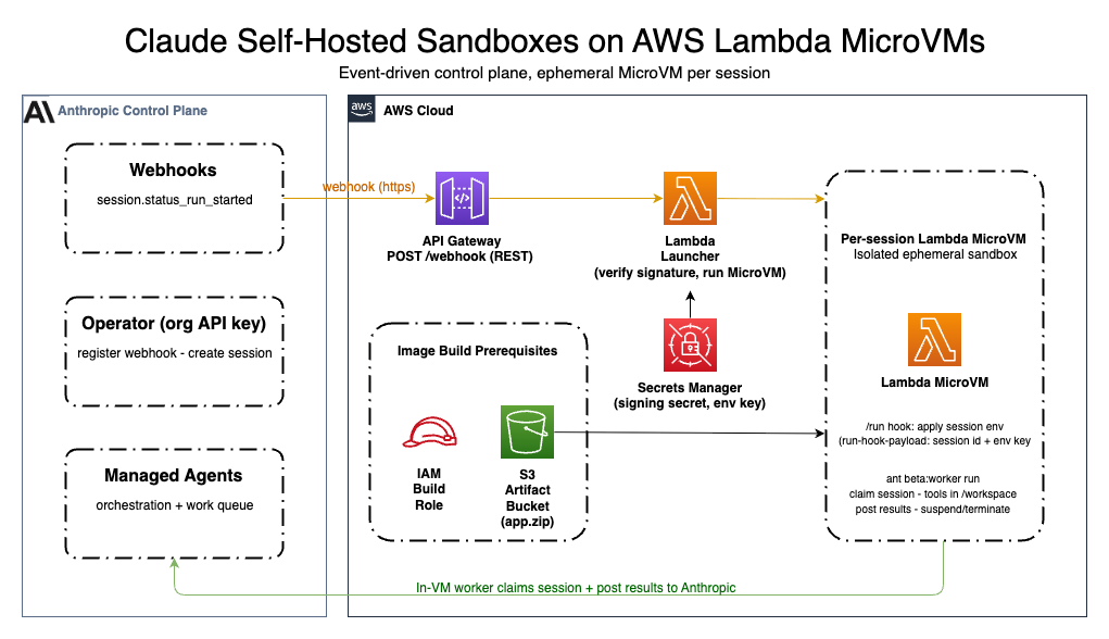
Figure 1: Reference architecture for self-hosted AI agent sandboxes on Lambda MicroVMs
The sample architecture is event-driven. The only inbound traffic is the webhook call. When the event arrives, the handler launches a MicroVM. Once launched, the MicroVM pulls its assigned session from the orchestration system’s work queue and runs the task. In our example, the developer’s “find slow queries” request has been queued as a session. The agent now needs to reach your infrastructure, spin up an isolated environment, and hand off the work. The following sequence shows how each component interacts to fulfill a single session.
The orchestration service queues work as sessions. A MicroVM launches to service each session, and the worker is the process running inside that MicroVM that claims the session, executes tool calls, and returns results.
- Once the orchestration service marks a session as ready to run, it sends a
session.status_run_startedwebhook to an Amazon API Gateway endpoint, triggering a MicroVM launch. - The launcher verifies the webhook signature using a signing secret from AWS Systems Manager Parameter Store, rejecting invalid or stale deliveries before spending compute.
- The launcher calls
RunMicrovm, passing the session ID and a secret reference throughrunHookPayload. It deduplicates on the webhook event ID (backed by Amazon DynamoDB) so retries do not launch duplicate VMs. - The MicroVM boots from a pre-captured Firecracker snapshot and receives the dispatch on its
/runlifecycle hook. The worker fetches the environment key from Parameter Store using its execution role. It pulls the matching session from the work queue, claims it, and executes tool calls in an isolated/workspacedirectory. When finished, it posts results and exits. The idle policy suspends then terminates the VM.
Deduplication. The webhook event ID serves as the idempotency key. The launcher uses Powertools for AWS Lambda (Python) with a DynamoDB persistence layer to verify exactly-once processing. If the orchestration application retries a delivery with the same event ID, Powertools protects the system from launching extra MicroVMs and doing extra work.
Credential boundaries. Each component accesses only the single secret it needs. The launcher reads only the webhook signing secret to verify inbound events. It passes only an ARN reference to the environment key into the MicroVM payload. The MicroVM’s execution role retrieves only that environment key at runtime. No single component holds both secrets.
| Component | Has access to |
| Launcher Lambda | Webhook signing secret (verify inbound events) |
| MicroVM worker | Environment key (through the execution role, to poll and claim sessions) |
Cost model. You pay for MicroVM run time per session, plus standard charges for API Gateway requests, Parameter Store API calls, and Lambda invocations for the launcher. When no sessions are active, no MicroVMs run. Cost scales with concurrent sessions and their duration, avoiding idle compute charges.
Implementation
The following sections explore the reference architecture in more depth.
Project structure
The reference solution uses AWS Serverless Application Model (AWS SAM) for infrastructure-as-code. Alternatively, if you use an AI coding agent such as Claude Code, Kiro, or Cursor, the Agent Toolkit for AWS includes a Lambda MicroVMs skill that gives your agent the procedures to provision, configure, and deploy MicroVM-based sandbox environments on your behalf.
Launcher: verify the webhook before spinning up compute
When the webhook arrives saying a developer’s session is ready, the launcher’s first action is signature verification. If it fails, the function returns 401 immediately. No MicroVM launches. No DynamoDB writes. You don’t pay for fraudulent or replayed requests.
After verification, the launcher builds a dispatch payload containing the session ID, environment ID, region, and an ARN reference to the environment key secret. It passes this to RunMicrovm through runHookPayload:
MicroVM worker: claim one session, execute, exit
The MicroVM image is built from a Firecracker snapshot. The worker process starts during image creation and is captured in the snapshot, so there is no application startup at run time. The /run lifecycle hook delivers the dispatch payload:
The worker acknowledges the hook within its timeout, fetches the environment key, and claims the session. This is where the requested work begins. The worker connects to the analytics database, runs EXPLAIN ANALYZE on the flagged queries, writes optimized alternatives to /workspace/suggestions.sql, and posts the results back to the developer. All of that happens inside this single VM. When the session completes, the worker calls terminate-microvm to release all compute resources.
Deployment
For full deployment instructions, see the reference solution README. Before deploying, make sure you have these prerequisites.
Prerequisites
- An AWS account with permissions for Amazon Simple Storage Service (Amazon S3), AWS Identity and Access Management (IAM), AWS Systems Manager Parameter Store, Amazon API Gateway, AWS Lambda, AWS WAF, Amazon CloudWatch Logs, and AWS Lambda MicroVMs.
- AWS Command Line Interface (AWS CLI) v2+.
- The AWS SAM CLI.
- An existing Anthropic Claude Managed Agents agent configured with a
self_hostedenvironment (note the agent ID and environment ID). - A webhook signing secret and environment key, both generated in the Anthropic Claude Console.
Four steps
- Deploy the control plane. Build and deploy the SAM stack, which creates the launcher Lambda, API Gateway endpoint, WAF WebACL, DynamoDB idempotency table, Parameter Store entries, and MicroVM execution role.
- Register the webhook and populate secrets. In the Claude Console, register the stack’s
WebhookUrloutput as a webhook endpoint subscribed tosession.status_run_started. Store the signing secret and environment key in the Parameter Store resources created by the stack. - Build the MicroVM image. Package the Dockerfile and worker code, upload to Amazon S3, and create the image. The service runs your Dockerfile, launches the worker, and captures a Firecracker snapshot. Monitor build progress in Amazon CloudWatch under
/aws/lambda/microvms/<image-name>. - Verify. Create a test session and confirm a MicroVM launches and completes end-to-end. The reference solution includes a verification script that creates a session, triggers the webhook, and validates the full flow.
Using Claude Platform on AWS (CPOA)
The preceding architecture works similarly when you access Claude through Claude Platform on AWS rather than the first-party API. Three things change in the worker:
- Client initialization. Replace the first-party client with the AWS client and supply your workspace ID:
- Authentication options. CPOA supports two modes:
- CPOA API key (
aws-external-anthropic-api-key-...): Store it in Parameter Store the same way as the first-party environment key. These keys are short-lived (12-hour STS tokens) and must be regenerated when they expire. - SigV4 (IAM): The MicroVM execution role can sign requests directly, so there is no secret to store or rotate. Set the environment key secret to a placeholder value (for example,
use-sigv4) and the SDK falls through to IAM credentials automatically. This is the recommended path for production.
- CPOA API key (
In both authentication modes, attach the AWS managed policy AnthropicSelfHostedEnvironmentAccess to the MicroVM execution role. This policy grants the aws-external-anthropic actions needed to poll the work queue, claim sessions, and post results. See IAM actions for Claude Platform on AWS for the full reference.
Prerequisite: Enable outbound web identity federation once per AWS account:
Everything else, including webhook verification, deduplication, credential separation, and idle policy remains the same.
Security
Earlier we talked about what goes wrong without isolation. Credentials exposed between sessions. Scripts unintentionally reaching production. Agents escaping their sandbox. This architecture implements defense in depth to help prevent these.
Each component accesses a single, scoped secret. The launcher passes only an ARN reference to the worker credential into the MicroVM. The MicroVM’s execution role retrieves only that credential at runtime. The analytics database connection string does not touch the launcher and does not leave your environment.
AWS WAF applies managed rule sets (OWASP, known bad inputs, IP reputation) and per-IP rate limiting. Amazon API Gateway request validation rejects malformed bodies. The launcher performs HMAC signature verification as the true authentication boundary.
Each session runs in its own MicroVM. Sessions do not share memory, disk, or network namespaces. Firecracker provides hardware-virtualization-based isolation. The launcher IAM role reads only the signing secret. The MicroVM execution role reads only the worker credential. Both are scoped to specific Parameter Store ARNs. The Amazon S3 artifact bucket blocks public access, enables versioning, and uses server-side encryption.
Conclusion
This post walked through how to give your internal AI agent a safe place to run database queries, generate code, and execute scripts on behalf of fifty developers without leaking data between sessions or reaching resources it shouldn’t.
AWS Lambda MicroVMs provide ephemeral, VM-isolated compute environments that align with the per-session execution model of AI agent sandboxes. Snapshot-based launch avoids application startup latency. Idle policies terminate VMs once sessions complete. Firecracker isolation verifies that sessions do not share state. You pay only for active execution time and maintain full control over credentials, networking, and governance within your AWS boundary.
You build and operate a serverless control plane. You get per-session VM isolation with no idle compute cost and no shared tenancy.
To get started, explore these resources:
- Read more about Lambda MicroVMs in the launch announcement post.
- Clone the reference solution in the aws-samples repository.
- Add the MicroVMs skill to your coding agent.
- Learn more about AWS Lambda MicroVMs in the Developer Guide.
- Learn about Anthropic self-hosted sandbox configuration in the self-hosted sandbox documentation.
- For more serverless learning resources, visit Serverless Land.
AI Is Not Exempt From the Law
Post Syndicated from The Atlantic original https://www.youtube.com/watch?v=lOI50oMkoHU
How CSIRO built scalable, cost-optimized genomic variant querying on AWS
Post Syndicated from Prof. Denis Bauer original https://aws.amazon.com/blogs/architecture/how-csiro-built-scalable-cost-optimized-genomic-variant-querying-on-aws/
This is a guest post by Denis Bauer, Yatish Jain, Anuradha Wickramarachchi, Brendan Hosking, and Nick Edwards of CSIRO, in collaboration with the ASP Prototyping and Scaling Team at AWS.
In this post, we describe how researchers at CSIRO, Australia’s national science agency, built Serverless Beacon (sBeacon), a scalable serverless solution for securely querying genomic variant data on AWS, underpinning production-scale clinical and research applications.
The Beacon protocol is the widely adopted standard for exchanging genomic and phenotypic data developed by the Global Alliance for Genomics and Health (GA4GH). It uses an API to define how data is shared, with the goal of enabling efficient and secure data discovery across international research and clinical networks.
sBeacon is a production-ready implementation of this standard, built using AWS services: Amazon Simple Storage Service (Amazon S3), AWS Lambda, Amazon DynamoDB, and Amazon Athena. By using these foundational AWS serverless services, sBeacon is able to provide the following benefits to researchers and clinicians needing to perform genomic variant querying:
- Highly scalable for large cohorts: sBeacon can scale to support hundreds of millions of individuals (and billions of genomic locations), which makes it suitable even for mega-biobank-scale datasets.
- Low cost to run: Because it uses a serverless, cloud-native architecture, sBeacon can operate for approximately USD 0.40 per month for a 1000 Genomes-scale dataset. The following case study breaks down ingestion, query, and storage costs in detail.
- High performance and fast query response: Real-world queries return in seconds (about 5 seconds) because of the serverless compute and efficient architecture, for near real-time data lookups.
- No heavy data ingestion or transformation needed: sBeacon can directly consume standard VCF files (a common format for genomic variant data), which reduces the need to load data into databases or transform it to different data structures.
- Rapid onboarding of new data: Genomic data generation is accelerating because it underpins clinical diagnosis and treatment, and because its complexity demands ever-larger cohorts to study complex traits. As a result, both clinical services and research cohorts must continuously onboard new data, and Beacon supports real-time generation-to-use life cycles (about 18 seconds).
- Improved privacy, data ownership, and decentralization: Because sBeacon doesn’t require central databases and supports federated networks, data stays under the control of original holders, which can help data custodians address privacy and ethical considerations in sensitive genomic and medical data sharing.
- Lower barrier to entry for broader participation: Its affordability, simplicity, and small operational footprint can help make it more accessible for smaller or resource-limited institutions and countries, which can increase participation from underrepresented populations and improve data diversity.
- Zero trust model: sBeacon enforces explicit authentication, least-privilege data access, ephemeral compute isolation, and strict cloud-native boundary controls that help confirm no component, user, or request is implicitly trusted.
Prerequisites
sBeacon is deployed as a container that sets up the necessary development environment, with Terraform defining the resources for the deployment. To get started, clone the terraform-aws-serverless-beacon repository on the GitHub website.
Make sure that your development environment contains Docker and has the necessary permissions for you to use it without super user access. Press Ctrl+Shift+P (Cmd+Shift+P on macOS) to open the command palette in VS Code, and then choose Reopen in Container. This opens the workspace in the container environment that we have defined.
Now, run the following command to initialize the necessary libraries and Lambda layers.
Next, run the following command to initialize the Terraform environment.
Optionally, you can define a backend by following the instructions in the repository. After the preceding command runs successfully, you can run the deployment command.
Enter yes when prompted to proceed with the deployment. After the deployment is complete, you receive information such as the API URL and the command to sign in as the admin or guest user. To shut down the entire service, run terraform destroy. Any created datasets are lost (but not the VCFs on which they are based).
Solution walkthrough
CSIRO developed sBeacon for sharing and querying genomic and medical data. sBeacon uses AWS serverless technology for the elastic scaling of compute resources.
The architecture of sBeacon performs two broad processes:
- Data onboarding: the ingestion and indexing of genomic metadata into sBeacon.
- Data querying: the querying of the genomic metadata by end users.
Data onboarding
During the onboarding process, you define where the genomic data and the metadata (such as disease status, age, and location) is located. Note that genomic data is not copied out of its original location but rather is referenced when needed. In contrast, metadata is loaded to sBeacon’s storage mechanisms because it is necessary to perform indexing that allows efficient querying. The user will need to ensure no sensitive or privacy-revealing data is disclosed. The example details the approach using CSIRO’s Ontoserver. However, sBeacon supports the API schema of the Ensembl OLS V4 specification.
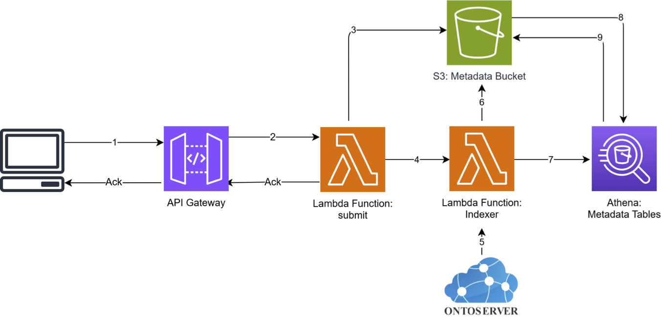
Figure 1. Data onboarding.
The data onboarding process is summarized by the following steps:
- The onboarding starts with the user submitting the location of the genomic data as request payloads to an API Gateway endpoint.
- The request payloads are forwarded to an AWS Lambda function that handles the data indexing.
- The metadata is written to an Amazon S3 bucket in the ORC format, to allow future querying and processing by Athena.
- An AWS Lambda function is called to orchestrate the indexing process.
- The CSIRO Ontoserver is called to build the ontology index for advanced metadata queries.
- The resulting index files are written to Amazon S3.
CREATE TABLE AS SELECT(CTAS) queries are run on Amazon Athena to build the metadata tables.- Athena loads the metadata from Amazon S3 into the metadata tables.
- The metadata tables are written back to Amazon S3 in ORC format.
Data querying
Querying in sBeacon is flexible, catering to a wide range of applications from human genetic disease to pathogen queries. We achieved this by designing the query architecture modularly. This approach let us separate the querying logic into several Lambda functions based on their querying scope, while maintaining a similar architecture.
The following architecture diagram describes the workflow for metadata querying, which uses the Variant Querying Module described later in this section.
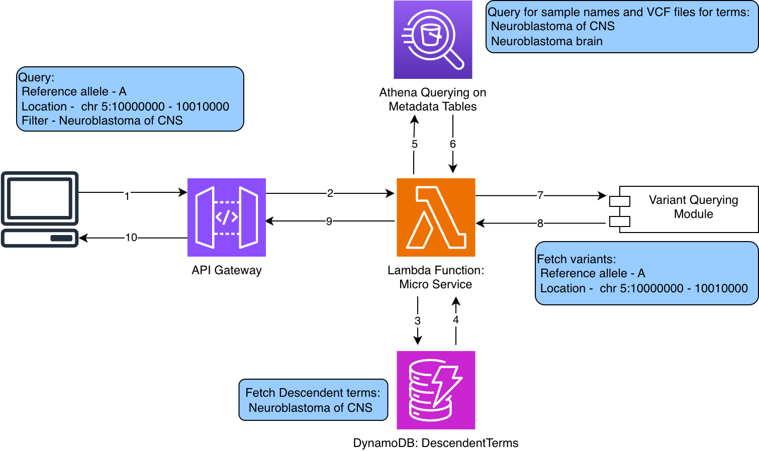
Figure 2. Data querying.
- The user submits their query to the API Gateway endpoint.
- API Gateway calls the Microservice Lambda function.
- The Microservice Lambda function looks up the relevant query ontology terms in an Amazon DynamoDB table.
- The matching ontology descendent terms (and their codes) are returned to the Microservice Lambda function. The descendent terms are those that match a hierarchical descendent of each term, or each term itself, from the query.
- Using the ontology codes from step 3, the metadata tables on Athena are queried.
- The metadata associated with the query is returned from Athena.
- If required by the query, the Microservice Lambda function queries the Variant Querying Module.
- The variant data associated with the genomic conditions in the query is returned to the Microservice Lambda function.
- The result is formatted according to the Beacon protocol and is returned to the user through Amazon API Gateway.
- The response is received by the user.
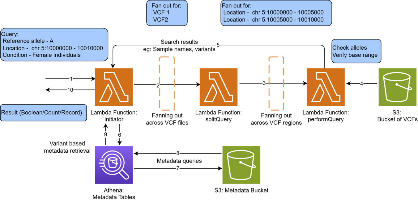
Figure 3. Variant Querying Module.
Genomic variant queries are performed using the Variant Querying Module. The workflow of this module is as follows:
- The Microservice Lambda function calls an Initiator Lambda function.
- The Initiator Lambda function fans out the
splitQueryLambda function across the VCF files. - The
performQueryLambda function is then fanned out across the VCF regions in each of the files involved in the query. - The
performQueryLambda function fetches the VCF files from Amazon S3. - The query results are synchronously returned to the parent Initiator Lambda function.
- If requested by the user, metadata can optionally be queried, where the Initiator Lambda function queries the metadata from Athena.
- Athena queries the metadata from Amazon S3 (through an external table).
- The metadata results are returned to Athena.
- The Initiator Lambda function receives the metadata from Athena.
- All the query results, including any optional metadata, are returned to the calling Microservice Lambda function.
Case study: 1000 Genomes dataset
We demonstrate sBeacon on chromosome 1 of the 1000 Genomes Project to report how it handles large-scale variant queries. We measure ingestion efficiency, query scalability, and cost for typical population-scale analyses, such as identifying SNP variants across defined genomic regions. The case study uses chromosome 1 (chr1, 8% of the genome) from the 1000 Genomes Project, which contains 2504 samples. This multi-sample VCF is approximately 1.1 GB compressed, with data stored in Amazon S3. Note that sBeacon can also process cohorts of single-sample VCF files. All costs in this section are for the Asia Pacific (Sydney) Region (ap-southeast-2), exclude applicable taxes, and reflect pricing at the time of writing.
sBeacon can ingest chromosome 1 from the 2504 individuals in 18 seconds, for less than 1 cent (USD 0.00052). This is because sBeacon does not copy the large genomic information but instead creates index files that enable random access. Cost is therefore driven predominantly by storing the copied metadata. After ingestion, sBeacon can be maintained for USD 0.000025 per month (1 MB of compressed metadata stored for 2504 samples in ORC format, plus genomic index files). If you store the genomic data as well, this would be USD 0.032 for chr1 (at USD 0.025 per GB in ap-southeast-2) or about USD 0.425 for the whole genome.
Query time is similarly near real time. For example, querying across a region of 10,000 base pairs to determine the genotypes in this region takes 1.52 seconds across the 2504 individuals. This would serve a query such as “Fetch all individuals with a specific BRCA1 mutation who have stage 3 cancer.” The cost for such a query is USD 0.00013. Note how the query time stays constant even with an increasing number of variants returned (for example, from 4 to 400).
Table 1. Query example costing and times (whole chromosome 1).
| Query region size (bases) | Number of variants found | Average Time | Compute Cost (per query in USD) |
| 10 | 4 | 1.51 s (+- 0.26) | 0.00013 |
| 100 | 18 | 1.52 s (+- 0.25) | 0.00013 |
| 1,000 | 84 | 1.62 s (+- 0.24) | 0.00014 |
| 5,000 | 229 | 1.65 s (+- 0.29) | 0.00014 |
| 10,000 | 400 | 1.52 s (+- 0.11) | 0.00013 |
Table 2. Cost for ingestion, querying, and idling (whole chromosome 1 for 2504 genomes with less than 10 MB of metadata).
| Scenario | Metric | Cost (USD) per month |
| Ingestion Cost | per 1000 ingestions | 0.53 (32.82 GB seconds of Lambda) |
| Query compute cost | per 1000 queries | 0.28 (9.8 GB seconds of Lambda) |
| Query Athena Cost | per 1000 queries | 0.05 |
| Idle Cost (Storage Cost) | 1.1 GB | 0.03 |
| Query DynamoDB Cost | Per 1000 queries | 0.0005 |
Security features
Security and compliance is a shared responsibility between AWS and the customer. AWS is responsible for protecting the infrastructure that runs the AWS services described in this post, and you are responsible for your use of those services, including how you configure them, which identities you grant access to, and which data you choose to onboard. Consider the services you choose carefully, because your responsibilities vary depending on the services used, how you integrate those services into your IT environment, and applicable laws and regulations. For more information, see the AWS Shared Responsibility Model.
Zero trust model
- Explicit authentication and authorization – Every API request must carry a valid JWT issued by the Amazon Cognito user pool (
aws_api_gateway_authorizer.BeaconUserPool-authorizer, typeCOGNITO_USER_POOLS). The authorizer runs at API Gateway before any Lambda function is invoked, so requests do not reach a handler without Cognito validation. Token validation includes signature, expiry, and audience (Cognito app client ID). You can disable authentication during the first deployment withBEACON_ENABLE_AUTH = falsefor intentionally public or open beacons. This is an explicit operator decision, not a default.
Authorization (what a valid user can do) is enforced inside the Lambda layer, not in Amazon API Gateway:
- Group membership (
sbeacon-record-access-user-group, and so on) controls the maximum granularity returned. - Admin-only operations (dataset submission, deletion) check for
sbeacon-admin-groupmembership before proceeding. - Least-privilege data access – sBeacon implements role-based access control (RBAC) through Cognito groups that map directly to disclosure tiers. You assign each user one or more of the following:
| Cognito group | Maximum disclosure |
sbeacon-boolean-access-user-group |
exists: true/false only |
sbeacon-count-access-user-group |
aggregate counts |
sbeacon-record-access-user-group |
full variant details and sample names |
sbeacon-admin-group |
preceding tiers plus dataset management |
The JWT carries the user’s group memberships as claims. The query Lambda function reads these claims to determine requested_granularity and include_details, then passes both flags to performQuery. performQuery computes only what was requested. A boolean-tier user’s request does not cause sample-level data to be computed or returned, even if it exists in the VCF.
- Ephemeral compute isolation – Lambda execution environments are stateless by design. Each cold start is a fresh container,
/tmp(1,024 MB forperformQuery) is cleared between cold starts, and concurrent invocations run in separate sandboxes with no shared memory. Thebcftoolssubprocess insideperformQueryruns and exits within the Lambda function lifetime (10 second timeout). No state persists after invocation. - Cloud-native boundary controls – API Gateway is the public entry point in this architecture. Amazon S3 buckets, DynamoDB tables, Athena, and Amazon SNS topics have no public resource policies. Amazon S3 buckets are created with private ACLs and
BucketOwnerPreferredownership controls. Lambda functions run on AWS-managed VPCs with no inbound network access. Amazon SNS topics are account-private (no external principal grants).
Privacy and data ownership
Each institution deploys the entire Terraform stack into its own AWS account, so there is no shared infrastructure, no central data lake, and no cross-account trust. VCF files live in the deploying institution’s Amazon S3 bucket and do not leave it. performQuery passes the Amazon S3 URL directly to bcftools as a subprocess argument, which uses htslib HTTP byte-range requests to read only the tabix-indexed region of interest (about 1 KB per query). The raw genomic sequence bytes do not pass through Lambda memory as returnable data. What the query returns upstream (exists as a boolean, call_count as an integer, and variant representations) is aggregate result data, not source sequence.
Decentralization in sBeacon is achieved at the storage layer, not the compute layer. The _vcfLocations registered for a dataset are Amazon S3 URIs, and these can point to buckets owned by entirely different organizations. When a query runs, performQuery passes each URI directly to bcftools, and htslib issues HTTP byte-range requests (Range: bytes=X-Y) against the Amazon S3 REST API of whichever organization owns that bucket. The raw VCF bytes do not leave the source organization’s Amazon S3 bucket. Only the query result (exists, count, or variant record) is returned.
Data onboarding privacy
The submitDataset endpoint sits behind the same API Gateway Cognito authorizer as all other endpoints. An unauthenticated request receives a 401 response before reaching any Lambda function. Beyond authentication, the handler also checks that the caller is a member of sbeacon-admin-group. A valid token from a user in only record-access or count-access is rejected. This means the beacon operator explicitly controls the set of people who can introduce data into the system, so onboarding is not a self-service capability.
Further considerations
We chose AWS Lambda over AWS Step Functions in this architecture because it can process much larger payloads. Given the size and complexity of genomic data and the fan-in and fan-out architecture for parallel handling, AWS Lambda emerged as the lower-cost and more flexible approach for this workload.
As demonstrated in the sBeacon publication, the architecture can cater to population-scale datasets. However, if you accidentally attempt to run a range query of the entire genome, the architecture times out at the Amazon API Gateway level. Applying functional operations over the whole genome requires further architectural considerations.
Because a single fan-out query spawns many parallel Lambda invocations, you need to monitor concurrency consumption to confirm that burst queries do not exhaust the account’s concurrency pool and starve other functions. Tracking the ConcurrentExecutions metric at both the account and function level provides early visibility into capacity pressure.
Similarly, because synchronous Lambda invoke does not automatically retry on throttle, a 429 response from a performQuery invocation means the result is silently lost unless the application handles it explicitly. Setting Amazon CloudWatch alarms on the Throttles metric for performQuery allows you to take corrective action, such as requesting a concurrency limit increase, before throttles affect query accuracy. Alternatively, we have produced a separate architecture that sends alert email with diagnostic information when Lambda functions fail, available in the error-catcher repository on the GitHub website. You can implement this in the repository or set it up as a standalone service to catch Lambda errors thrown by sBeacon.
After idle periods, simultaneous performQuery invocations might encounter cold starts that add latency to query responses. Enabling provisioned concurrency on the query-path Lambda functions helps reduce this cold-start latency during burst fan-out scenarios at the price of increasing the idle cost.
Conclusion
In this post, we described how CSIRO built sBeacon, a fast, scalable, and low-cost way to run genomics workloads on AWS. sBeacon implements the GA4GH Beacon standard with a fully serverless and modular architecture. This publicly available solution supports near real-time querying of standard VCF data, scales to mega-biobank cohorts, minimizes ingestion effort, and supports privacy and zero-trust security. If you are considering genomics on AWS, you can deploy sBeacon on existing Amazon S3-hosted VCF data, integrate it with clinical or research workflows through the Beacon API, and progressively federate with other Beacons for secure, cross-institutional genomic data discovery. Set up sBeacon to query your genomic data and explore the possibilities of securely sharing insights with your collaborators. You can read more about sBeacon in our publication: Scalable genomic data exchange and analytics with sBeacon. The source code for sBeacon can be downloaded from our GitHub repository.
About the authors
[$] Looking forward to Git 2.56 — and 3.0
Post Syndicated from corbet original https://lwn.net/Articles/1094575/
The Git source-code management system is
at the core of development processes worldwide, so changes, especially
incompatible changes, are of great interest to the developers involved.
The Git 2.56 release, which can be expected around the end of September, is
currently available in release-candidate form. It
is not the most earth-shaking of releases, but the one that follows, which
might be the long-awaited Git 3.0, may well be.
Systemtap 5.6 released
Post Syndicated from corbet original https://lwn.net/Articles/1095220/
Version 5.6 of the Systemtap tracing tool has been released.
BPF LSM hooks and XDP packet-processing probes for the –bpf
runtime, BTF-based kernel.tracepoint probes, statement execution
tracing, a new @enumname() operator, richer runtime error context,
dyninst hardware watchpoints, modern systemd service templates, and
broad Linux 7.2 runtime/tapset compatibility work. Multithreaded
speedups throughout.
Security updates for Friday
Post Syndicated from corbet original https://lwn.net/Articles/1095219/
Security updates have been issued by AlmaLinux (.NET 10.0, coreutils, kernel, libevent, libsoup3, microcode_ctl, perl-Net-DNS, postgresql18, postgresql:16, postgresql:18, tomcat, and unbound), Debian (bind9, chromium, libapache2-mod-auth-openidc, nginx, xz-utils, and zip), Fedora (chromium, freeipmi, GitPython, gnatcoll, nodejs-undici, parted, python-django5, and sblim-cmpi-base), Mageia (imagemagick and python-starlette), Oracle (.NET 10.0, .NET 8.0, .NET 9.0, coreutils, corosync, firewalld, kernel, libevent, libsoup, microcode_ctl, nginx:1.24, perl, perl:5.32, postgresql:16, postgresql:18, redis, rsync, rsyslog, tesseract, and unbound), Red Hat (vim), SUSE (alsa, chirp, chromium, cjose, cups, discount, firefox, gh, glibc, gvfs, jq, kernel, libcjose-devel, libmbedcrypto7, libpcap, mbedtls-2, netcdf, nodejs18, openai-codex, openvpn, pcre2, perl-net-dns, sngrep, tiff, and znc), and Ubuntu (bison, bubblewrap, and gst-plugins-good1.0).
Padma Lakshmi talks about the impact of her high-profile career
Post Syndicated from The Atlantic original https://www.youtube.com/shorts/zaP7tce_EN0
A Conversation With Gina Raimondo
Post Syndicated from The Atlantic original https://www.youtube.com/watch?v=J52fDKpeUjY