Network connectivity patterns for private access to Amazon OpenSearch Serverless used to require considerable setup. You had to create virtual private cloud (VPC) endpoints in every consumer VPC and configure Amazon Route 53 Profiles for cross-account DNS. You also had to maintain custom private hosted zones with CNAME records and deploy resolver inbound endpoints for on-premises connectivity. The next generation of OpenSearch Serverless changes this. It uses standard AWS PrivateLink interface endpoints with native private DNS support. Connectivity patterns that previously required multi-step DNS orchestration now work with the same endpoint mechanics you already use for other AWS services.
Collections use resource-based endpoints on the on.aws domain in two formats. The per-collection endpoint (<collectionId>.aoss.<region>.on.aws) reaches a single collection, and the hostname itself identifies which collection you want, so no additional routing information is needed. The per-account Regional endpoint (<accountId>.aoss.<region>.on.aws) reaches any collection in your account through one hostname. Because the hostname alone does not identify a specific collection, you add the x-amz-aoss-collection-name header (or x-amz-aoss-collection-id) to each request to name the target collection. The AWS SDKs include this header automatically when they sign the request with Signature Version 4 (SigV4).
Both formats use standard AWS PrivateLink. You create the VPC endpoint from the Amazon Virtual Private Cloud (Amazon VPC) console or the Amazon Elastic Compute Cloud (Amazon EC2)CreateVpcEndpoint API, using the service name com.amazonaws.<region>.aoss-data. It is the same interface endpoint you create for any other AWS service.
In this post, each pattern shows the architecture, the DNS resolution flow, and the data traffic path. Patterns 1 through 8 operate within a single Region across one or more accounts, labeled Region A in the diagrams, so the repeated Region A boxes in a cross-account pattern are the same Region. Only Pattern 9 spans Regions, shown as Region A and Region B.
These patterns apply to the collection (data) endpoint only. When you create a collection, you also receive an OpenSearch UI endpoint. That endpoint uses a separate PrivateLink mechanism today, with its own VPC endpoint and access policy, and is on a path to move to the standard PrivateLink model. OpenSearch UI connectivity is out of scope for this post.
When you create a standard VPC endpoint for com.amazonaws.<region>.aoss-data with private DNS enabled, AWS creates a private hosted zone for *.aoss.<region>.on.aws and associates it with your VPC. This zone maps collection hostnames to the endpoint’s private elastic network interface (ENI) IP addresses. Your compute’s DNS query reaches the VPC’s Amazon Route 53 Resolver at VPC+2, which resolves the hostname to ENI IPs.
One endpoint serves every collection hostname in the Region. The following AWS CLI command creates that interface endpoint, and the --private-dns-enabled flag turns on the private DNS resolution described here.
OpenSearch Serverless has no per-collection Dashboards endpoint. Use OpenSearch UI applications to explore and visualize collection data.
The diagrams in the following patterns use an Amazon EC2 instance to represent the compute client. Any compute in the VPC reaches a collection the same way, including EC2 instances, AWS Lambda functions attached to the VPC, and containers on Amazon Elastic Container Service (Amazon ECS) or Amazon Elastic Kubernetes Service (Amazon EKS). The connectivity, DNS resolution, and access policies are the same regardless of the compute type.
Pattern 1: Private access from a single VPC
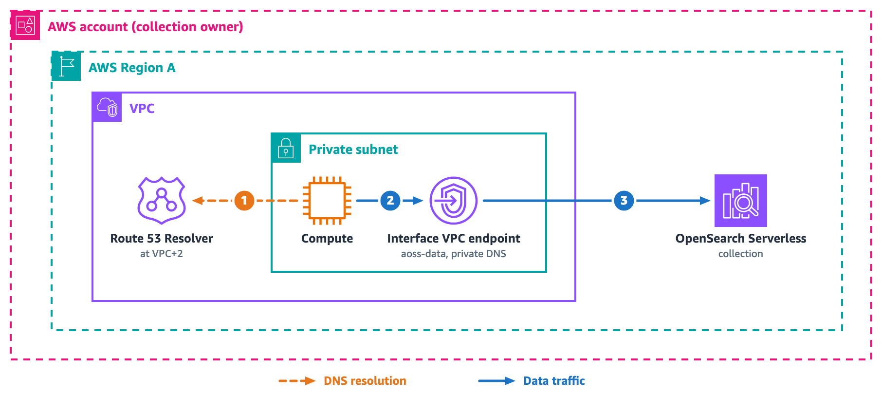
Compute in a VPC needs private access to collections in the same account. The following diagram shows the architecture for private access from a single VPC.
Figure 1: Private access from a single VPC
Create a standard VPC endpoint in the VPC where your compute runs, then reference its ID in the collection’s network policy.
For the DNS resolution flow, (1) compute queries <collectionId>.aoss.<region>.on.aws, and the VPC Route 53 Resolver at VPC+2 returns the endpoint ENI IP addresses because private DNS is enabled on the endpoint.
For the data traffic path, (2) compute connects to the ENI, and (3) PrivateLink forwards the request to the service, which routes to the collection by hostname.
Pattern 2: Multiple VPCs in the same account
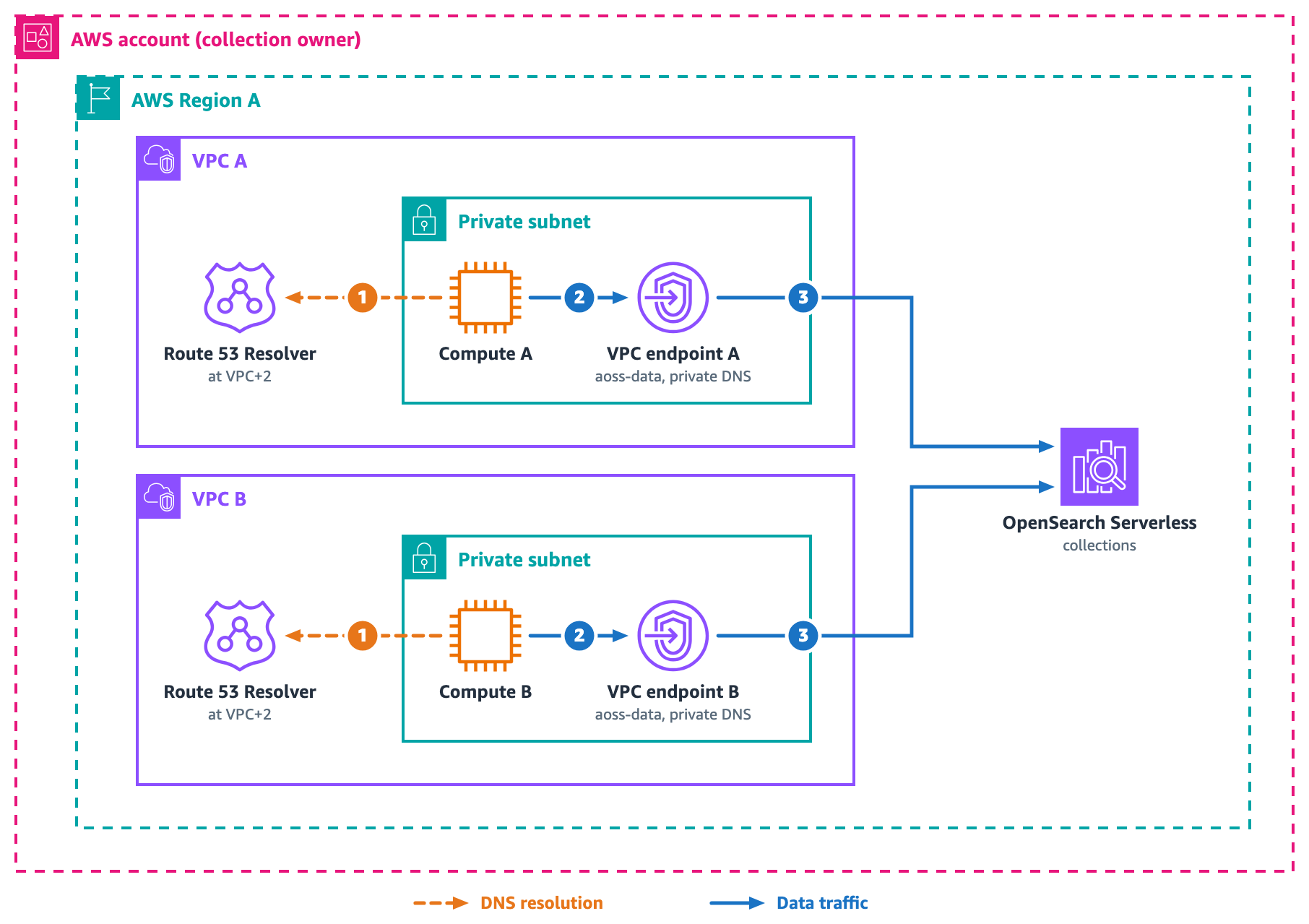
Several VPCs, split by environment, tier, or team, need private access to the same collections. The following diagram shows how each VPC uses its own endpoint to reach the same collections.
Figure 2: Multiple VPCs in the same account
Each VPC needs exactly one aoss-data endpoint with private DNS enabled, and that single endpoint already reaches every collection in the Region. DNS resolves independently within each VPC, so there is no cross-VPC DNS dependency. Adding a new VPC takes two steps. Create the endpoint, then add its endpoint ID to the collection’s network policy. Do not create a second aoss-data endpoint with private DNS enabled in the same VPC. Both endpoints share the same private hosted zone, which causes a conflict and the creation fails.
For the DNS resolution flow, (1) compute in each VPC queries the collection hostname, and that VPC’s Route 53 Resolver at VPC+2 returns the endpoint ENI IP addresses because private DNS is enabled on the endpoint.
For the data traffic path, (2) compute connects to its local ENI, and (3) PrivateLink forwards the request to the service, which routes to the collection by hostname.
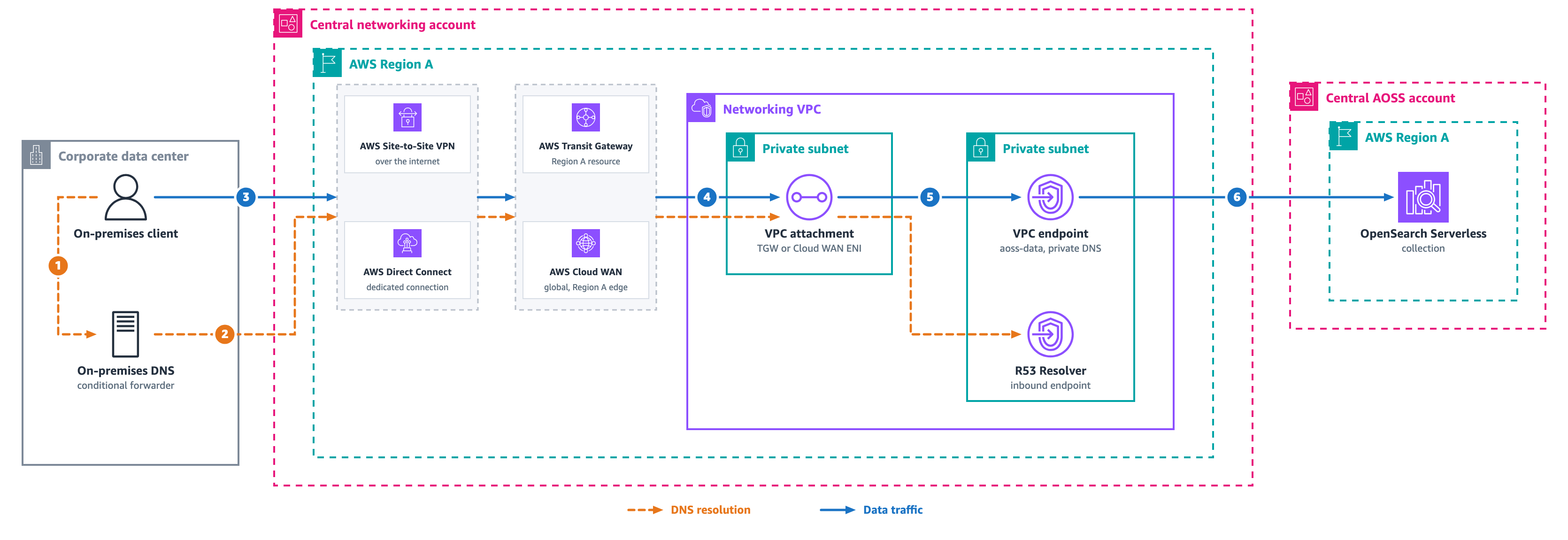
Pattern 3: On-premises access from a single account
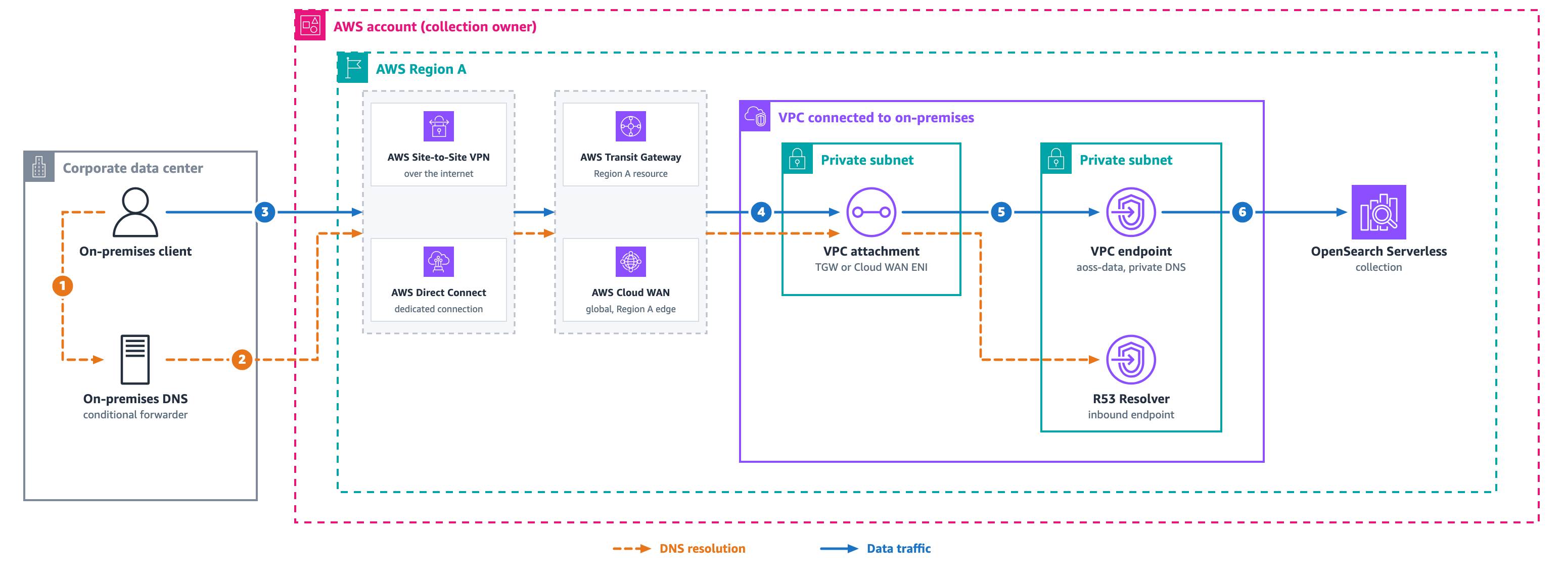
Figure 3: On-premises access from a single account
On-premises DNS servers sit outside the VPC and cannot resolve PrivateLink private DNS names directly. Place an Amazon Route 53 Resolver inbound endpoint in the VPC that holds the aoss-data VPC endpoint. On-premises DNS forwards queries for aoss.<region>.on.aws to that inbound endpoint. The inbound endpoint resolves them against the private hosted zone. The inbound endpoint’s security group must allow TCP/UDP port 53 from your on-premises resolver ranges.
For the DNS resolution flow, (1) the client queries the on-premises resolver. (2) The on-premises conditional forwarder for *.aoss.<region>.on.aws sends the query over Direct Connect or VPN, through Transit Gateway or Cloud WAN, to the inbound endpoint. The inbound endpoint uses the VPC Route 53 Resolver to return the endpoint’s private ENI IPs.
For the data traffic path, (3) the client sends an HTTPS request with the Transport Layer Security (TLS) Server Name Indication (SNI) header set to the collection hostname, over Direct Connect or VPN through Transit Gateway or Cloud WAN. (4) Traffic crosses the VPC’s attachment ENI, (5) reaches the VPC endpoint ENIs, and (6) PrivateLink forwards the request to the service.
Pattern 4: Cross-account access with an endpoint in each consumer VPC
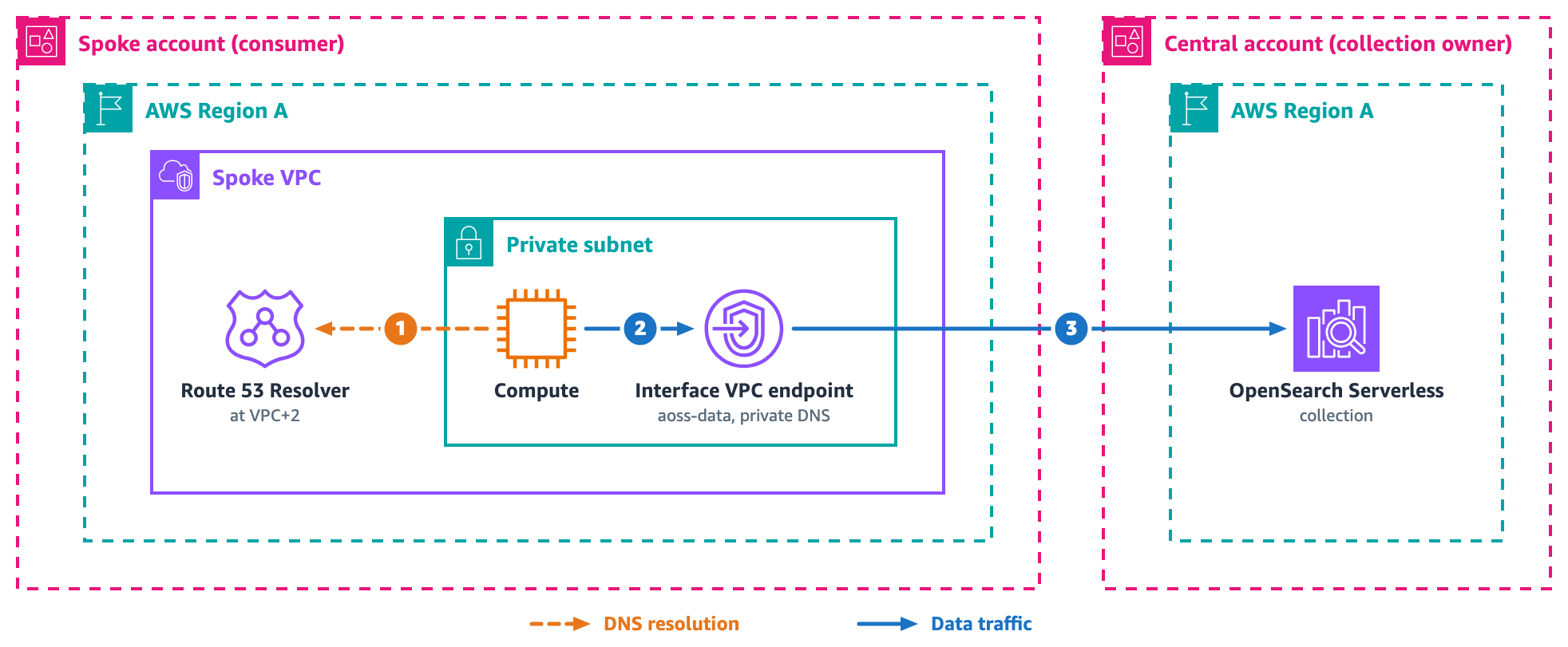
A central account hosts collections, and compute in spoke accounts needs private access. Many enterprises start here. The following diagram shows the cross-account endpoint architecture.
Figure 4: Cross-account access with an endpoint in each consumer VPC
Each spoke creates its own endpoint. The collection owner’s network policy references the spoke’s endpoint ID. The data access policy grants the spoke’s IAM role. PrivateLink carries the traffic end to end, with no Transit Gateway and no peering.
The endpoint lives in the spoke account, not the collection account. The spoke team creates a standard interface VPC endpoint in the spoke VPC for the service name com.amazonaws.<region>.aoss-data with private DNS enabled. The collection owner does not create this endpoint. After the endpoint is ready the spoke shares its endpoint ID with the collection owner, who adds that ID to the collection network policy under SourceVPCEs. A network policy accepts endpoint IDs from accounts across your organization. Each spoke creates its own endpoint and shares the ID rather than peering VPCs or routing through another account’s endpoint.
Network access and data access stay separate. The network policy authorizes the endpoint, and the data access policy authorizes the identity. A serverless data access policy grants principals from the collection’s own account. For a spoke in another account, you create an IAM role in the collection account and grant that role in the data access policy. The spoke role then assumes it to sign requests.
The following network access policy lists the two spoke endpoint IDs under SourceVPCEs and sets AllowFromPublic to false, so only those endpoints reach the collection and the policy denies public access.
For the DNS resolution flow, (1) spoke compute queries the VPC Route 53 Resolver at VPC+2, which returns the local endpoint ENI IPs because private DNS is enabled on the endpoint.
For the data traffic path, (2) compute connects to the local ENI. (3) PrivateLink forwards the request to the service, which checks the network policy for the endpoint ID and the data access policy for the IAM role before routing. Adding a spoke takes one API call and two policy edits.
Pattern 5: Centralized shared endpoint with Amazon Route 53 Profiles over Transit Gateway
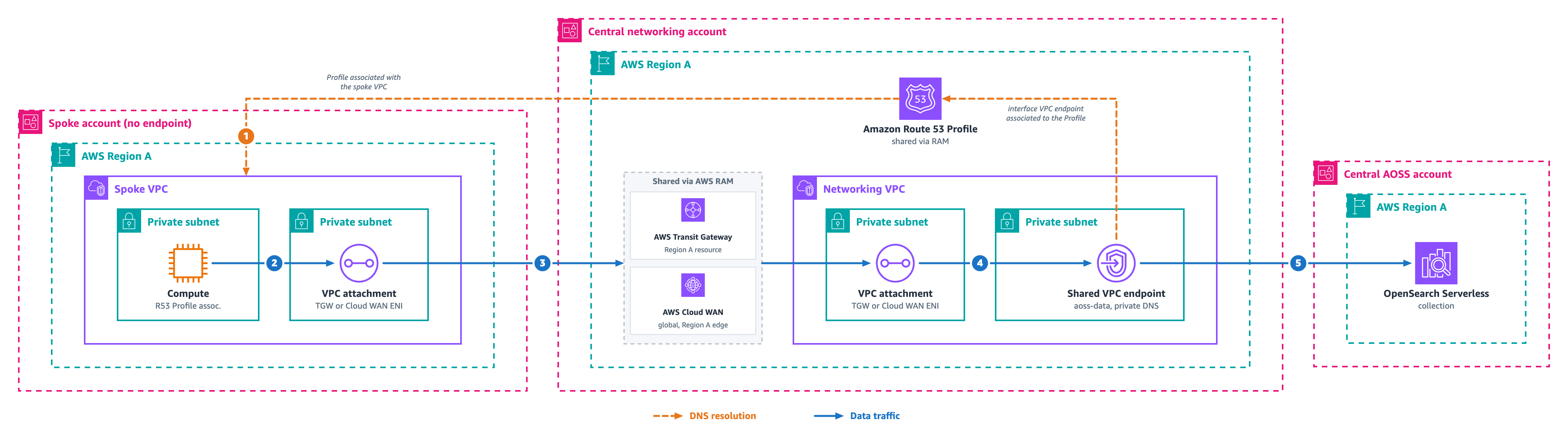
You want fewer PrivateLink endpoints, so you run one shared endpoint in a networking VPC and reach it from spoke accounts over Transit Gateway or AWS Cloud WAN, with no endpoint in each spoke. The following diagram shows this centralized architecture.
Figure 5: Centralized shared endpoint with Amazon Route 53 Profiles over Transit Gateway
Pattern 5 consolidates access through a single shared endpoint in a central networking VPC rather than creating one per spoke. Because spoke VPCs have no local endpoint, they cannot resolve *.aoss.<region>.on.aws on their own. You share the endpoint’s private DNS with spoke VPCs using Amazon Route 53 Profiles, shared through AWS Resource Access Manager (AWS RAM). This is the one pattern where you still manage DNS propagation.
For the DNS resolution flow, (1) the spoke resolves the hostname through the shared Route 53 Profile, which returns the networking-VPC endpoint ENI IPs.
For the data traffic path, (2) traffic leaves the compute through the spoke VPC’s attachment ENI, (3) crosses Transit Gateway or Cloud WAN into the networking VPC’s attachment ENI, (4) reaches the shared endpoint ENIs, and (5) PrivateLink forwards the request to the service.
Pattern 6: Cross-account centralized networking with on-premises
A central account hosts collections. A separate networking account owns Direct Connect or VPN and Route 53. On-premises clients reach the collections through the networking account. The following diagram shows this architecture.
Figure 6: Cross-account centralized networking with on-premises
The networking account runs the standard VPC endpoint and a Route 53 Resolver inbound endpoint. The collection owner’s network policy references the networking account’s endpoint ID.
For the DNS resolution flow, (1) the on-premises client queries its resolver. (2) The on-premises conditional forwarder sends the query over Direct Connect or VPN, through Transit Gateway or Cloud WAN, to the inbound endpoint. The inbound endpoint uses the VPC Route 53 Resolver to return the endpoint’s private ENI IPs.
For the data traffic path, (3) the client sends HTTPS over Direct Connect or VPN, through Transit Gateway or Cloud WAN. (4) Traffic crosses the networking VPC’s attachment ENI, (5) reaches the networking-VPC endpoint ENIs, and (6) PrivateLink forwards the request to the service in the central account. The two teams coordinate through one artifact, the endpoint ID.
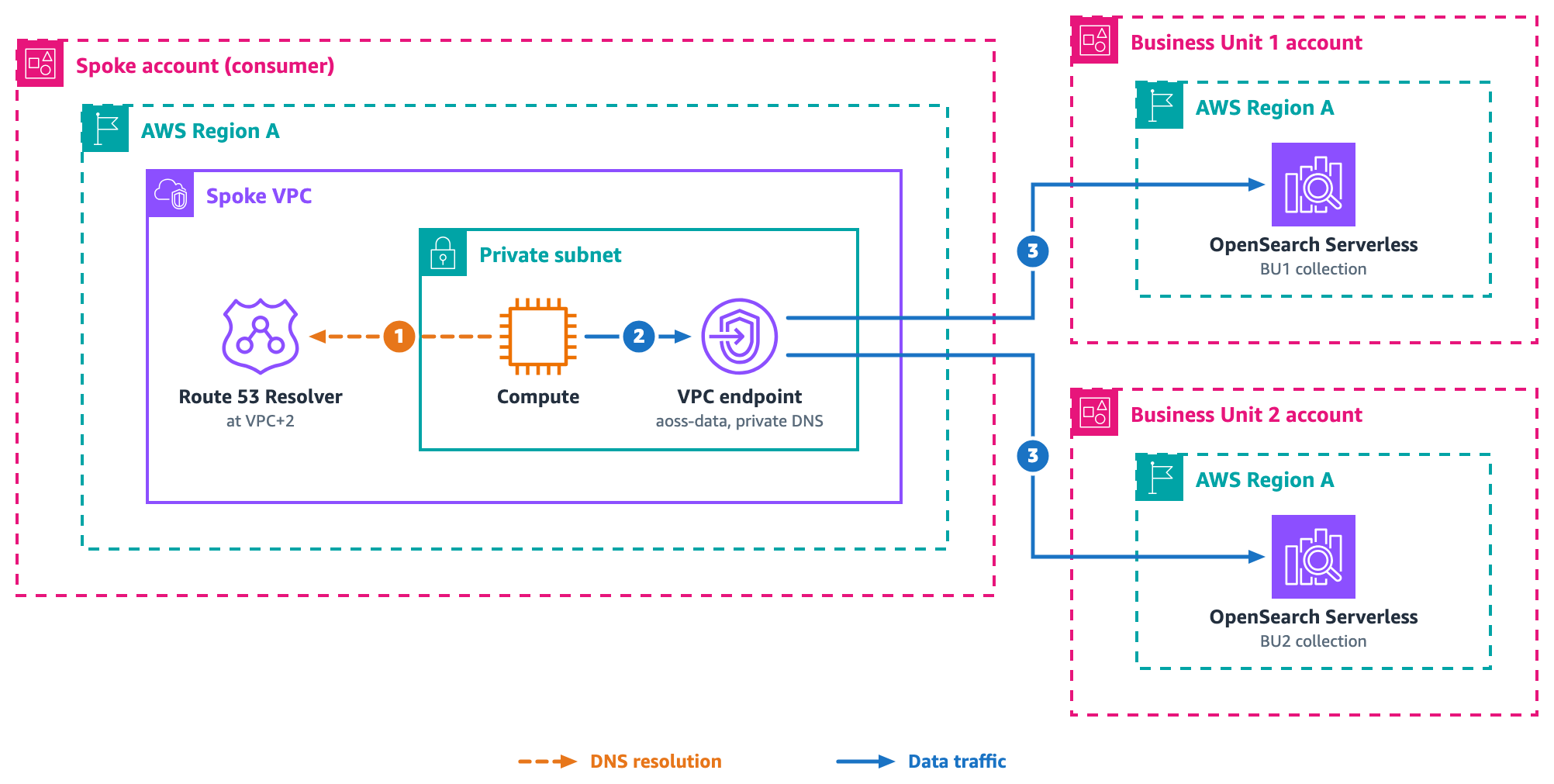
Pattern 7: Distributed multi-business-unit with spoke-account access
Spoke accounts such as analytics or application teams need collections spread across several business unit accounts, and each unit manages its own collections. The following diagram shows the distributed multi-business-unit architecture.
Figure 7: Distributed multi-business-unit with spoke-account access
Each spoke creates one standard endpoint, which resolves every collection hostname in the Region. Each business unit’s network policy lists the spoke endpoint IDs. Access control decides which collections a spoke reaches. DNS does not.
For the DNS resolution flow, (1) spoke compute queries the VPC Route 53 Resolver at VPC+2, which returns the endpoint ENI IPs because private DNS is enabled on the endpoint.
For the data traffic path, (2) compute connects to the local ENI, and (3) PrivateLink forwards the request to the service, which routes to the correct business unit collection by hostname.
Action
Required change
New collection in any BU
No networking change is needed because in the network policy collection/* wildcard, already covers any new collection
New spoke account
Spoke creates an endpoint, and BUs add its ID to their policies
Remove spoke access
BUs remove the endpoint ID and the IAM principal
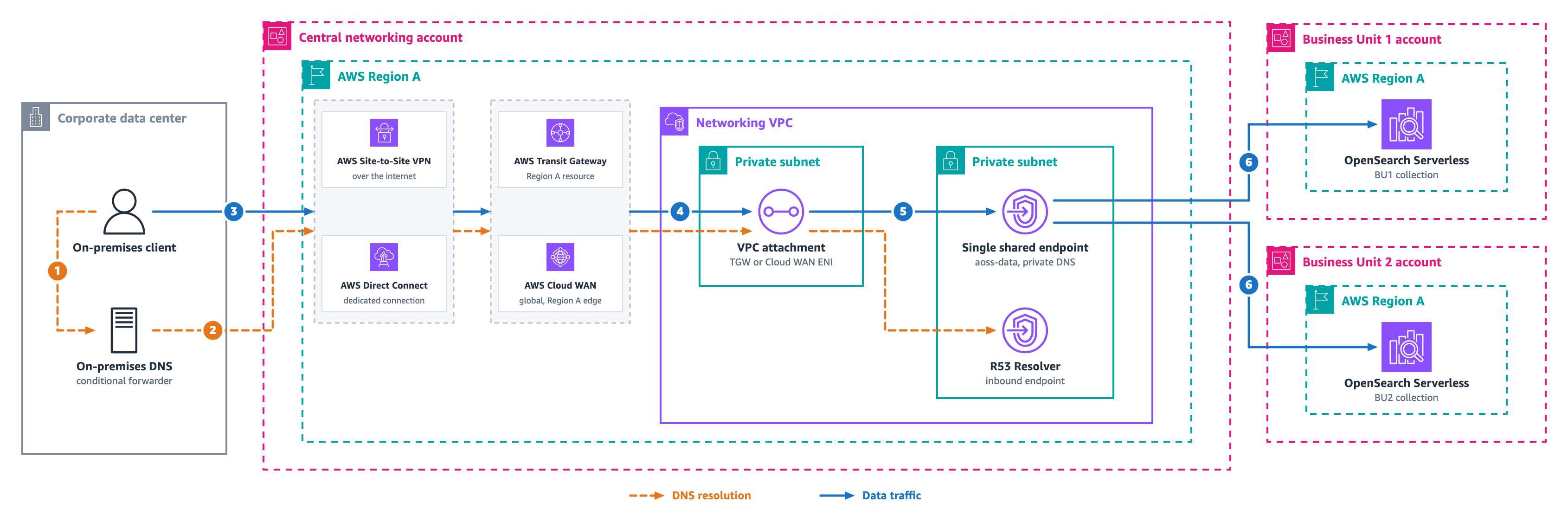
Pattern 8: Distributed multi-business-unit with on-premises access
Several business units own collections in separate accounts. On-premises clients reach collections across all of those accounts through a central networking account. The following diagram shows this architecture.
Figure 8: Distributed multi-business-unit with on-premises access
The networking account runs one standard endpoint that resolves *.aoss.<region>.on.aws hostnames, regardless of which account owns the collection. Each business unit’s network policy includes the networking endpoint ID.
For the DNS resolution flow, (1) the on-premises client queries its resolver. (2) The on-premises conditional forwarder for *.aoss.<region>.on.aws sends the query over Direct Connect or VPN, through Transit Gateway or Cloud WAN, to the networking VPC’s inbound endpoint. The inbound endpoint uses the VPC Route 53 Resolver to return the shared endpoint’s private ENI IPs.
For the data traffic path, (3) the client sends HTTPS over Direct Connect or VPN, through Transit Gateway or Cloud WAN. (4) Traffic crosses the networking VPC’s attachment ENI, (5) the request arrives at the shared endpoint ENIs, and (6) the service routes to business unit 1 or business unit 2 by hostname, as long as that business unit’s policy lists the networking endpoint ID. Adding a collection in any business unit needs no networking change if the network policy uses a collection/* wildcard, since the wildcard already covers it.
Pattern 9: Cross-Region access strategies
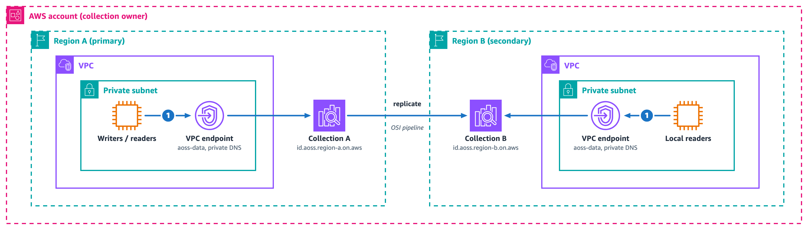
Consumers in Region B need data that lives in collections in Region A. The following diagram shows cross-Region access strategies.
Figure 9: Cross-Region access strategies
Collections are Regional. No built-in cross-Region endpoint or replication exists. Deploy independent collections in each Region, each with its own endpoint and policies, then synchronize data with one of these approaches.
Dual-write. The application writes to both Regions at ingestion time.
Amazon OpenSearch Ingestion pipeline. A pipeline replicates index operations to the secondary Region with near real-time lag. The pipeline creates its own PrivateLink endpoint to the destination collection. It adds the endpoint to that collection’s network policy automatically. You only need to name the network policy and grant the pipeline role.
Amazon Simple Storage Service (Amazon S3) Cross-Region Replication with re-ingestion. Cross-Region Replication copies objects, and an OpenSearch Ingestion pipeline loads them into the local collection. Lag runs in minutes, at the lowest cost of these approaches.
For the DNS resolution flow, DNS resolves locally in each Region, the same as Pattern 1. Each collection hostname carries its Region, so a hostname in Region A resolves through Region A’s own endpoint and a hostname in Region B resolves through Region B’s own endpoint, with no cross-Region DNS.
For the data traffic path, (1) compute in each Region uses that Region’s own endpoint to reach its local collection. Writes land in the primary Region and the sync approach you choose replicates them to the secondary Region, where local readers query the replica. The replicate arrow shows that cross-Region movement, such as an OpenSearch Ingestion pipeline that writes into the secondary-Region collection.
Scale-to-zero changes the economics. An idle secondary-Region collection costs only storage until requests arrive.
Summary
Pattern
Components
1. Same VPC
Standard endpoint and network policy
2. Multiple VPCs
Endpoint per VPC and a policy listing all IDs
3. On-premises
Endpoint, Route 53 inbound endpoint, on-premises forwarder, and Transit Gateway or Cloud WAN
4. Cross-account
Endpoint per consumer, network policy, and data policy
5. Centralized shared endpoint
Shared endpoint, Route 53 Profiles through RAM, and Transit Gateway or Cloud WAN
6. Central networking with on-premises
Networking endpoint, Route 53 inbound, forwarder, Transit Gateway or Cloud WAN, and policies
7. Multi-BU with spoke access
Endpoint per spoke, and each BU policy lists spoke IDs
8. Multi-BU with on-premises
One networking endpoint reached through Transit Gateway or Cloud WAN, and each BU policy lists its ID
9. Cross-Region
Independent collections per Region and a data-sync approach
Across each private pattern, the VPC endpoint resolves all *.aoss.<region>.on.aws hostnames through standard PrivateLink private DNS. Network policies control which endpoints reach a collection, and data access policies control which principals operate on the data. Only Pattern 5 asks you to manage DNS.
Cost considerations
The connectivity pattern you choose drives recurring cost, so match it to your scale instead of adding infrastructure you do not need. The two charges that come up most often, a Route 53 Resolver inbound endpoint and Route 53 Profiles, are both optional for access that stays inside AWS.
A Route 53 Resolver inbound endpoint is needed only for the on-premises patterns (3, 6, and 8), where an on-premises resolver forwards queries into the VPC. Traffic that stays inside AWS never uses it. Route 53 Profiles apply only when a VPC has no endpoint of its own, as in Pattern 5, where the profile carries the shared endpoint’s private DNS to the spoke. When each VPC runs its own interface endpoint, DNS resolves locally through the VPC Route 53 Resolver at no extra charge, so neither the inbound endpoint nor a profile is required.
For most multi-account and multi-Region deployments, an interface endpoint in each consumer VPC (Pattern 4) is the least complex and often the least expensive option. You pay for the interface endpoints you already need for private access, and local DNS resolution adds nothing. Because collections are Regional and each Region resolves on its own, this scales across Regions with no cross-Region DNS.
Centralizing on one shared endpoint (Pattern 5) lowers the number of interface endpoints. However, it adds Transit Gateway or Cloud WAN data processing charges and the cost of sharing DNS. You share that DNS either through Route 53 Profiles or through a private hosted zone that you associate across accounts and maintain yourself. A smaller endpoint count is not automatically cheaper because transit data processing can exceed the savings. Compare both designs against your own traffic before you decide.
OpenSearch Serverless uses standard AWS PrivateLink for private connectivity. You create a VPC endpoint, enable private DNS, and reference the endpoint ID in your network policy. The model scales from single-VPC access to multi-account and multi-business-unit designs, and only Pattern 5 adds DNS infrastructure, where you share the endpoint’s private DNS with Route 53 Profiles. The per-account regional endpoint goes further and serves any collection in an account through one hostname and connection pool. To get started, create your first collection in the OpenSearch Serverless console, or explore the OpenSearch Serverless documentation for detailed API references and tutorials.
Moovit, part of Mobileye (Nasdaq: MBLY), is a leading Mobility-as-a-Service (MaaS) solutions provider and the creator of a leading urban mobility app. Moovit’s iOS, Android, and web apps offer users a smart mobility experience to get to their destination using any mode of public and shared transportation. Transit riders can benefit from mobile ticketing to plan, pay, and ride with transit services. Introduced in 2012, Moovit now serves over 1.7 billion users in more than 3,500 cities across 112 countries, in 45 languages.
Behind these user-facing experiences is a data platform that processes large volumes of mobility, application, and operational data to support product analytics, business intelligence (BI), monitoring, and data science. As the platform grew, Moovit needed to keep analytical workloads reliable and cost-efficient without slowing down teams that depend on fresh data every day.
Over several years, Moovit’s Amazon Redshift cluster grew continuously. It started with an expanding fleet of DC2 nodes, migrated to RA3 nodes, and scaled multiple times to keep pace with growing data demands, ultimately becoming the backbone of their entire data platform.
To address this growth, Moovit transformed their data architecture by building an optimal multi-engine lakehouse architecture and assigning each workload to the most suitable option. This modernization reduced their Amazon Redshift cluster by 50 percent, while establishing a flexible, multi-engine architecture ready for future use cases.
In this post, we share how Moovit gained visibility into workload patterns, cleaned up unnecessary load, selected candidates for offloading, and ran a successful proof of concept (POC) on Amazon EMR Serverless. Moovit ultimately divided the workload between multiple engines, building a modern and cost-optimized data platform that combines provisioned Amazon Redshift, Amazon Redshift Serverless, and Amazon EMR.
The challenge: Outgrowing a single-engine data platform
The Amazon Redshift engine handled a wide variety of workloads, including:
Heavy ETL processing: Raw data ingestion from Amazon Simple Storage Service (Amazon S3) followed by complex aggregation pipelines (daily user-aggregation running once per day with a 3-day lookback, and weekly 10-day-lookback jobs).
Near-real-time operational monitoring: Queries executing every 20 minutes against raw data for system-health dashboards.
Business-intelligence reporting: Tableau extracts and live dashboards.
Data-science workloads: Exploratory analysis and model-feature engineering.
Ad-hoc analysis: Non-recurring queries done by analysts and engineers.
With business growth, storage grew by orders of magnitude over the past decade as the platform expanded. All these varied workloads competed for the same engine and pushed it to its limits. Jobs experienced increasing queue times, service level agreements (SLAs) were at risk, and adding nodes provided minimal performance gains, creating a need to isolate workloads.
Gaining visibility: Measuring workload impact
Moovit’s first modernization milestone was to create a trusted measurement foundation before changing any workloads. Instead of treating warehouse activity as a single opaque stream, the team implemented automated query attribution that continuously classified each query by workload owner and execution context. The classification combined multiple signals: who executed the query (user or service account), recognizable query-signature patterns, and metadata emitted by orchestration frameworks and scheduled processes.
This produced a historical, query-level map of platform usage that answered three critical questions: who is generating load, whatkind of workload is running, and how expensive each workload is in runtime and resource terms. With that baseline in place, the team made offload decisions from evidence rather than assumptions. This approach prioritized the largest and most stable optimization opportunities first and reduced the risk of moving business-critical workloads without visibility.
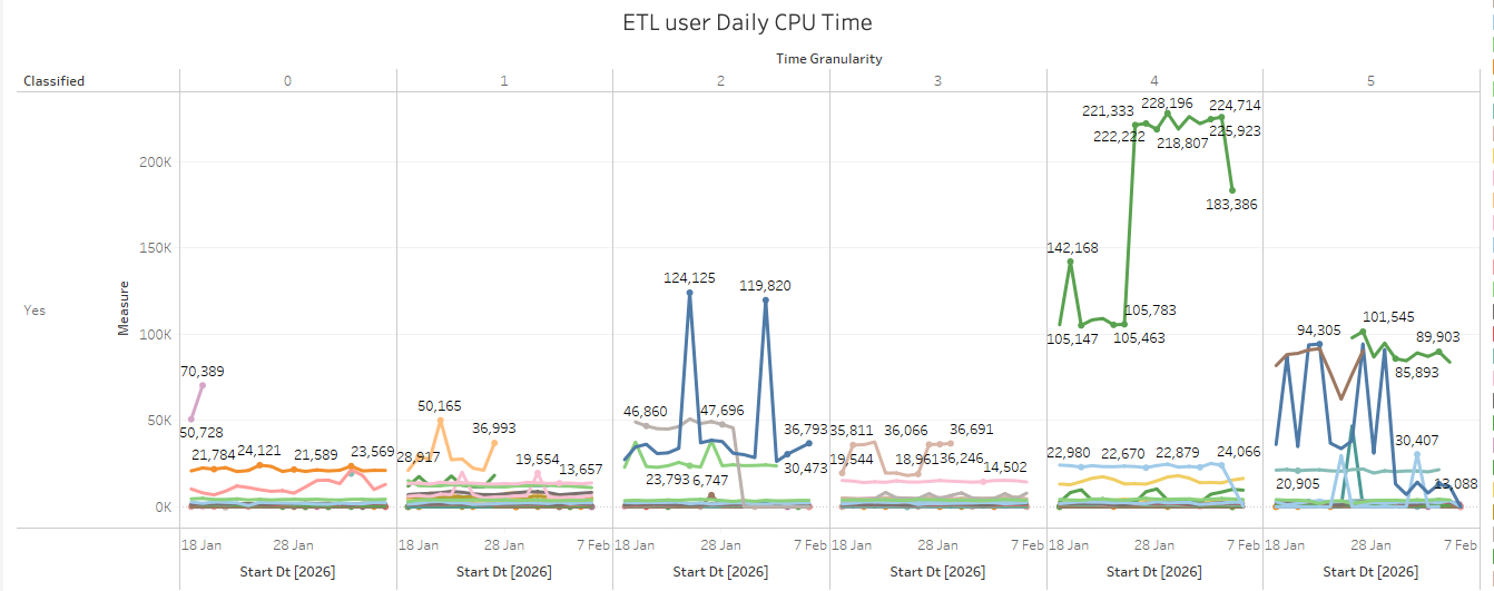
These classifications and workload metrics were reflected in a Tableau report that aggregated query activity by classification label and execution context. The view exposed operational dimensions such as classification, time granularity, service class, execution-time bucket, unload flags, and sample-query context, supporting both trend monitoring and root-cause drill-down.
The worksheet was parameterized to support multiple measurement modes over the same grouped workload population: total execution time, execution plus queue time, total CPU time, average execution time per query, and ratio-based efficiency views (execution/CPU and CPU/execution). This let the team compare “heavy by volume” workloads against “inefficient by behavior” workloads without creating separate artifacts.
For decision-making, CPU time was used as the primary impact metric because it best represented sustained compute pressure. Execution time, queue time, query-count normalization, and workload-management segmentation were treated as secondary evidence to distinguish:
compute-heavy but healthy workloads
queue-constrained workloads
high-frequency/low-cost workloads
noisy or weakly classified workloads that required attribution cleanup first
Using this framework, prioritization became systematic: first improve classification coverage, then rank workloads by CPU contribution, then validate with queue and workload management (WLM) signals, and finally choose the action path per workload (optimize SQL, reschedule, isolate, retire, or move to another engine).
The following figure shows an example of one of the dashboard widgets (CPU time by query).
Figure 1: CPU time by query, highlighting the most resource-intensive queries and their usage patterns
Cleanup: Reducing unnecessary data warehouse load
With a long-running data platform, in most cases the workloads will start accumulating, some of which become irrelevant at some point. For example, a report which was created and scheduled, yet it became irrelevant after a few years, but still running since no one disabled it. It’s important to indicate these workloads in general to reduce unnecessary load, yet even more critical before doing any significant architectural changes or migrations. Before migrating any workloads, Moovit first reduced unnecessary warehouse load.
The team:
Removed unused processes that were still consuming cluster resources.
Reduced unnecessary frequency where possible: some jobs ran more often than downstream consumers needed.
Reviewed workload-management guardrails to verify resource allocation matched actual priorities.
This cleanup phase was a prerequisite to migration. By removing waste first, the team verified that the workloads eventually selected for offloading were genuinely heavy rather than simply unoptimized or unnecessary.
The no-longer-relevant processes consumed around 7 percent of overall CPU time and were removed before the optimization work began.
Workload selection: Choosing what to offload
With a clear picture of workload patterns, Moovit faced a common decision point: continue scaling the existing Redshift cluster, or re-architect towards a multi-engine approach. The team evaluated two main paths:
Re-architect with Redshift multi-cluster and data sharing: Identify workloads that could benefit from resource isolation, then redistribute processing and queries between multiple Redshift clusters, combining both serverless and provisioned options. This would redistribute load across use-case-optimized clusters and potentially save costs through better resource use.
Re-architect with purpose-built engines: Identify workloads that could benefit from alternative processing frameworks and offload them to more suitable engines. This would reduce pressure on Amazon Redshift while building a more flexible, cost-efficient architecture.
Moovit decided to do both, because while some workloads benefited from being offloaded, others benefited from isolated Amazon Redshift compute.
The measurement data revealed a primary candidate for offloading: raw-data aggregation pipelines. This workload loaded raw data into Amazon Redshift from Amazon S3, then performed heavy sessionization and aggregation transformations. Raw tables were still used for ad-hoc and exploratory analysis, but recurring production consumers primarily depended on aggregated outputs, making these transformations strong candidates for offloading.
Proof of concept: Offloading to EMR Serverless with Spark SQL
With target workload identified, Moovit initiated a POC using Amazon EMR Serverless with Spark SQL. The choice of EMR Serverless was driven by several factors:
Spark SQL compatibility: The existing Redshift SQL logic could be ported with minimal changes to Spark SQL syntax.
Serverless simplicity: No cluster-management overhead during the evaluation phase.
Data-lake native: Processing could occur directly on data in Amazon S3.
The POC defined quantified success criteria measured over five or more consecutive runs:
Runtime reduction: Greater than or equal to 40 percent reduction for the transform portion of selected pipelines.
Amazon Redshift cost reduction: Greater than 30 percent reduction in Redshift RA3 compute with no performance degradation for remaining workloads.
Data-quality parity: Exact match between Spark and Amazon Redshift outputs on row counts, distinct users, and all published metrics over a frozen parity window.
Overcoming initial performance challenges
The first POC attempts exposed significant challenges. Early Spark jobs with 100 executors took approximately 4 hours, far exceeding the 30–40-minute baseline on Amazon Redshift. Beyond raw performance, the team encountered memory pressure, data-parity gaps between Spark and Amazon Redshift outputs, and subtle SQL behavior differences between the two engines.
The team systematically diagnosed and resolved these issues:
Execution-plan analysis: Reviewing the Spark execution plan revealed suboptimal query patterns that generated excessive data shuffles.
Query rewrites: Rewriting specific SQL constructs to align with Spark’s distributed processing model, including splitting large monolithic logic into staged transformations.
Reducing or rewriting expensive DISTINCT patterns: Identifying and eliminating unnecessary DISTINCT operations that created heavy shuffle pressure.
After applying these optimizations, execution time dropped from 4 hours to approximately 10 minutes, and the required executors dropped to fewer than 50, surpassing the original performance.
Validation: Ensuring data parity before cutover
Before transitioning any workload to production, Moovit implemented a rigorous validation process. The new Spark output was compared with the previous Amazon Redshift output using multiple dimensions:
Row counts: ensuring no data was lost or duplicated.
Metric parity: all published business metrics matched.
Daily trends: time-series patterns remained consistent.
Row-level checks: spot-checking individual records for correctness.
Only after all validation checks passed consistently over multiple consecutive runs did the team proceed with cutover for each workload.
Moving to production: Expanding workload offloading
With a successful POC demonstrating both performance gains and cost savings, Moovit progressively moved additional workloads from Amazon Redshift to EMR:
Heavy-aggregation jobs: The primary daily and weekly aggregation pipelines transitioned fully to EMR.
Data-transformation stages: Preprocessing steps that previously consumed Redshift compute moved to Spark, with only final aggregated results loaded back into Amazon Redshift for BI consumption.
Weekly batch workloads: Large batch jobs that previously created resource contention during weekend processing windows.
The transition used a measured approach: each workload was migrated individually, with data-quality validation confirming parity before decommissioning the equivalent jobs which were running on Redshift.
Additional optimizations: Redshift Serverless, workload isolation, and Amazon EMR on Amazon EC2
Beyond EMR offloading, Moovit implemented further architectural improvements to isolate workloads and optimize costs.
With heavy workloads successfully offloaded and isolated, Moovit proceeded to right-size the Redshift cluster. Rather than a single resize, the team reduced the cluster incrementally, two nodes at a time, using elastic resize. At each step, they validated that:
Existing BI workloads maintained acceptable performance.
Queue wait times remained within SLA thresholds.
No workload degradation was observed under peak loads.
This iterative approach minimized risk and allowed the team to find the optimal cluster size with confidence.
Workload isolation with Redshift Serverless
Amazon Redshift persisted as the engine of choice for serving curated BI data. However, not all Amazon Redshift workloads needed provisioned capacity:
Ad-hoc analyst queries: Moved to Redshift Serverless, isolating unpredictable workloads from the provisioned cluster through data sharing.
Data-science workloads: Transitioned to Redshift Serverless for flexible exploration without impacting production.
This workload isolation through Redshift Serverless provided resource separation without requiring additional provisioned capacity. The architecture now used data sharing to provide a unified view across provisioned and serverless clusters.
Operational isolation refinements
Moovit also refined workload isolation by rebalancing WLM priorities on the provisioned cluster. Because the ETL queue mainly handled raw data loading from Amazon S3 (which was not the bottleneck after heavy aggregations moved to Spark), its priority was reduced. At the same time, with most human users moved to Redshift Serverless, Tableau serving workloads on provisioned Redshift were prioritized higher to keep dashboard performance predictable. The final result: a 50% reduction in provisioned Redshift capacity.
Transitioning to EMR on EC2
EMR Serverless proved efficient for the POC phase: it allowed fast iteration without cluster management overhead. However, for longer-term recurring production workloads, Moovit moved to EMR on EC2 to better fit their production cost and infrastructure model, using existing compute reservations.
The transition between EMR deployment options required zero application code changes, demonstrating the flexibility of the EMR deployment options.
AI-assisted SQL translation
Additionally, Moovit used AI-assisted development tools, Claude Code and Cursor, to accelerate parts of the SQL transition process. These tools helped engineers identify Redshift SQL and Spark SQL syntax differences, suggest rewrites, and debug migration issues, while validation and production approval remained under engineer review.
Results: A modern multi-engine architecture
The architectural modernization delivered measurable outcomes:
Cluster size reduction: Redshift cluster size reduced to 50 percent of the initial capacity.
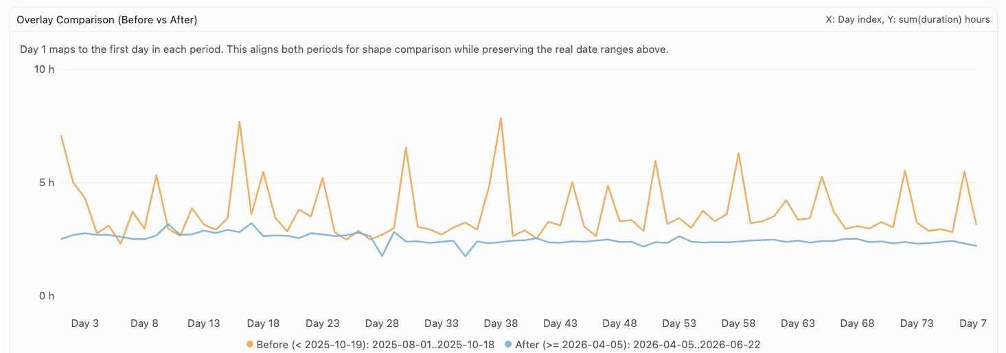
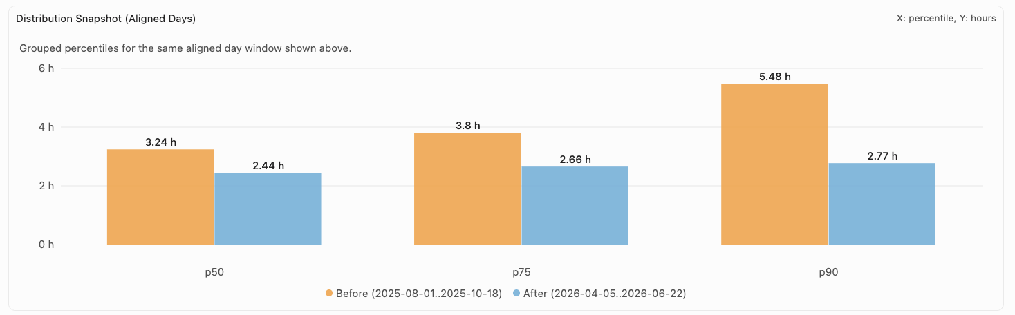
Performance improvement: Key aggregation jobs ran faster and more consistently on EMR (50 percent execution time reduction for p90).
Workload isolation: No single workload type could impact others through resource contention.
33 percent overall data pipeline cost reduction: Combined savings from cluster reduction, transition to EMR, and efficient serverless usage.
Future flexibility: The multi-engine architecture provided pathways for additional use cases without architectural changes.
The following figures compare aggregation-job performance before and after the transition.
Figure 2: Aggregation-job execution times before and after the transition
Figure 3: Wall-clock time for job executions by percentile, before and after the transition
The resulting architecture assigned each workload to the engine that fits it best:
Workload type
Engine
Rationale
Heavy ETL and aggregation
Amazon EMR (Spark SQL)
Distributed processing on Amazon S3. No data warehouse load required
Ongoing processing and BI reporting
Amazon Redshift provisioned
24/7 running processes
Ad-hoc queries
Amazon Redshift Serverless
Burst capacity with workload isolation
Data science
Amazon Redshift Serverless
Flexible exploration without impacting production
Lessons learned
The Moovit modernization journey produced several key insights applicable to similar architectural transitions:
Measure before you move: Establishing baseline metrics and automated classification was essential for identifying true offloading candidates. Without granular workload-level measurements, the team would not have identified which specific processes were exhausting the cluster.
Clean up before you migrate: Reducing unnecessary load first verified that migration efforts targeted genuinely heavy workloads rather than simply unoptimized or unused processes.
Small SQL changes, big impact: Moving from Redshift SQL to Spark SQL required relatively minor syntax adjustments. The core business logic remained intact, and most transformations translated directly with minimal refactoring.
Optimize for the engine: Porting SQL queries to Spark without optimization produced initially poor results for some workloads. Understanding Spark’s distributed execution model and optimizing for it was critical for achieving target performance.
Validate rigorously: Multi-dimensional data-parity checks (row counts, distinct users, metrics, daily trends, and row-level spot checks) gave the team confidence to cut over without data-quality regressions.
Moving between EMR options is straightforward: EMR Serverless proved very efficient for starting fast and evaluating Spark. When Moovit needed to move to EMR on EC2 to use existing reservations, the transition required no application code changes.
Iterative cluster rightsizing: Rather than a single resize, Moovit reduced the Redshift cluster incrementally (two nodes at a time) using elastic resize, validating performance at each step before proceeding further.
Conclusion
Looking ahead, as another potential optimization, Moovit will be evaluating the new Amazon Redshift RG instances for provisioned clusters, providing up to 2.2x better price performance and priced 30% lower than RA3, powered by AWS Graviton.
The broader takeaway is that AWS provides multiple purpose-built engines that can be used in a single data platform. In Moovit’s case, the biggest improvement came from assigning each workload to the engine that fit it best: Amazon Redshift for curated analytical serving, Redshift Serverless for isolated exploratory workloads, and Amazon EMR for large-scale transformations over data in Amazon S3. This architecture gives Moovit a foundation for future optimization and flexibility as data volumes grow and new analytical use cases emerge.
Tiered-memory systems are built with multiple types of memory, each of
which has different performance characteristics. In addition to the usual
DRAM, a tiered system might also provide faster high-bandwidth memory or
slower CXL memory. On these systems, the placement of memory allocations
has a significant effect on the performance that a workload will obtain.
While work on tiered-memory improvements has been ongoing for years, it
feels like the pace has slowed a bit recently. Even so, there are a few
efforts underway, but they are facing questions about whether the tiering
design makes sense.
Version
4.0 of the Audacity audio editor has been released. Notable changes in this
release include a rewritten interface using Qt, ability to save user-interface
layouts as “Workspaces”, improvements in working with audio clips, and a new .aup4 project format.
The release is not fully feature-compatible with the Audacity 3.x
series; see the compatibility
notes for a list of missing features.
Continuous improvement depends on experimentation. Teams know that the fastest path to better outcomes is to test changes against real user behavior, measure results, and iterate. In practice, sustaining that cycle is slow and costly because the overhead compounds with each attempt.
Three barriers slow teams down:
1. Planning cost — Turning a proposed change into a testable experiment requires defining a feature flag strategy, coordinating implementation, and wiring everything together before any user sees new behavior.
2. Measurement disconnected from action — Once live, teams must configure metrics, define success criteria, monitor, and interpret results. When metrics regress, remediation traditionally depends on a human merging a fix or rolling back a deployment.
3. Stalled iteration — Without a record of which change caused which outcome, the next hypothesis is a guess, so iteration often does not happen and the goal stalls.
This post introduces a reference solution that closes the gap between defining a goal and reaching it. A team states an improvement goal (for example, increase add-to-cart rate by 10%), and agents plan the experiment, implement the change, deploy it behind a feature flag, measure its impact, and iterate on the result, all within defined safety boundaries. The solution connects Kiro for code generation, AWS DevOps Agent for orchestration and release readiness review, and LaunchDarkly for feature flag governance, experiments, and Guarded Releases for safe, metric-driven rollouts with automatic rollback. The architecture described here is a reference implementation you can build today. A more turnkey experience is planned for the future.
Pre-requisites
Step 1. Enable AWS DevOps Agent and Create an Agent Space. AWS DevOps Agent is available in the AWS regions listed here. Follow these steps to create your AWS DevOps Agent and create an Agent Space.
Step 3. Enable the LaunchDarkly MCP Server in the Agent Space. AWS DevOps Agent connects to LaunchDarkly’s hosted MCP server as a client, giving it the ability to query flag state, read targeting rules, and list flags by project or environment.
Step 4 — Register the LaunchDarkly MCP server (account-level). MCP servers are registered at the AWS account level and shared among all Agent Spaces in that account.
Sign in to the AWS DevOps Agent console.
Navigate to the Capability Providers page (side navigation).
Find MCP Server under the Available providers section and choose Register.
Description: LaunchDarkly feature flag management MCP server
Enable Dynamic Client Registration: Select this checkbox to allow DevOps Agent to automatically register with LaunchDarkly’s authorization server
Step 4a — Configure the authorization flow
LaunchDarkly’s hosted MCP server uses OAuth for authentication:
Select OAuth 3LO (Three-Legged OAuth).
Choose Next.
Complete the OAuth authorization — you will be redirected to LaunchDarkly’s consent page to authorize the connection.
Choose Next.
Tip: Refer to the LaunchDarkly MCP server documentation for specific OAuth scope and credential details.
Step 4b — Review and submit
Review the MCP server configuration details.
Choose Submit.
AWS DevOps Agent validates the connection to LaunchDarkly’s MCP server.
On successful validation, the MCP server is registered at the account level.
Step 5 — Add the MCP server to your Agent Space
After the account-level registration, connect it to your specific Agent Space:
In the AWS DevOps Agent console, select your Agent Space (created in Section 1).
Go to the Capabilities tab.
In the MCP Servers section, choose Add.
Select the LaunchDarkly MCP server you just registered.
Configure tool access:
Allow all tools — makes all LaunchDarkly MCP tools available to the agent
Select specific tools — allowlist only the tools you need (recommended for production)
Choose Add.
Step 5 — Validate the connection. Run a test query to confirm the integration is working. In the DevOps Agent console, start a new investigation or chat session and ask: “List the feature flags in the <your-project-key> project in the production environment.” If the agent returns flag data from LaunchDarkly, the connection is active.
Solution overview
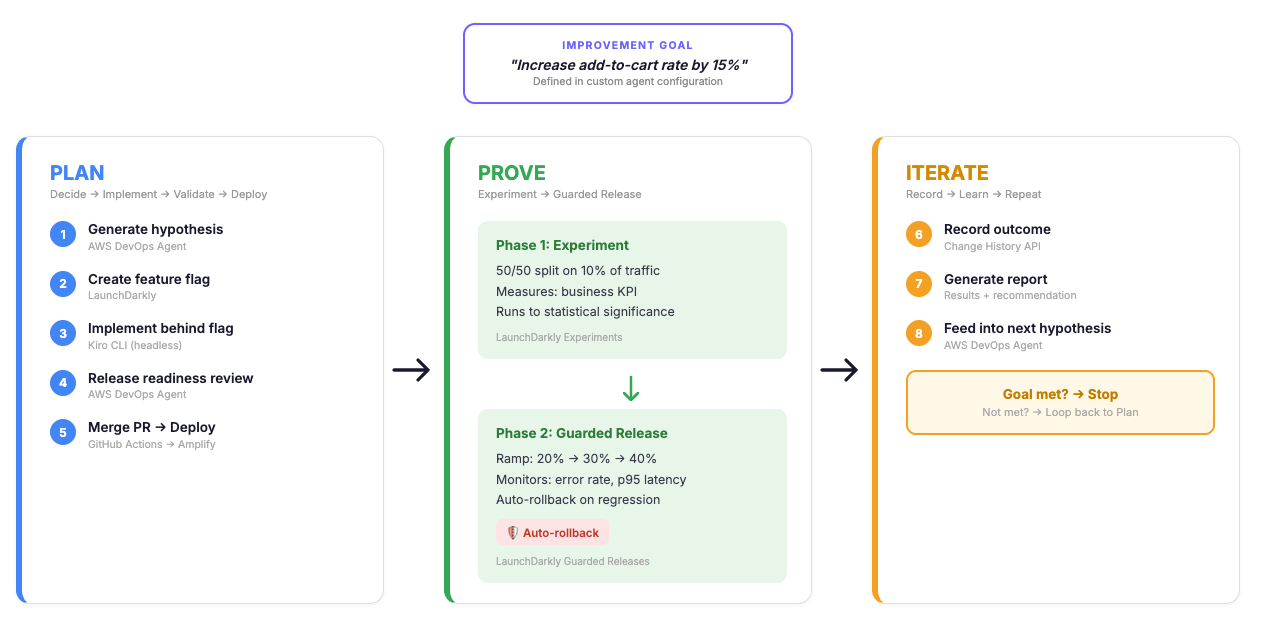
The automated experimentation lifecycle operates as a closed loop. A team states an improvement goal, and the system moves through a continuous cycle: decide what to try next, implement the change behind a feature flag, validate and deploy it, run an experiment to measure impact, roll it out safely, and feed the outcome back into the next iteration. The loop continues until the goal is met or the team decides to stop.
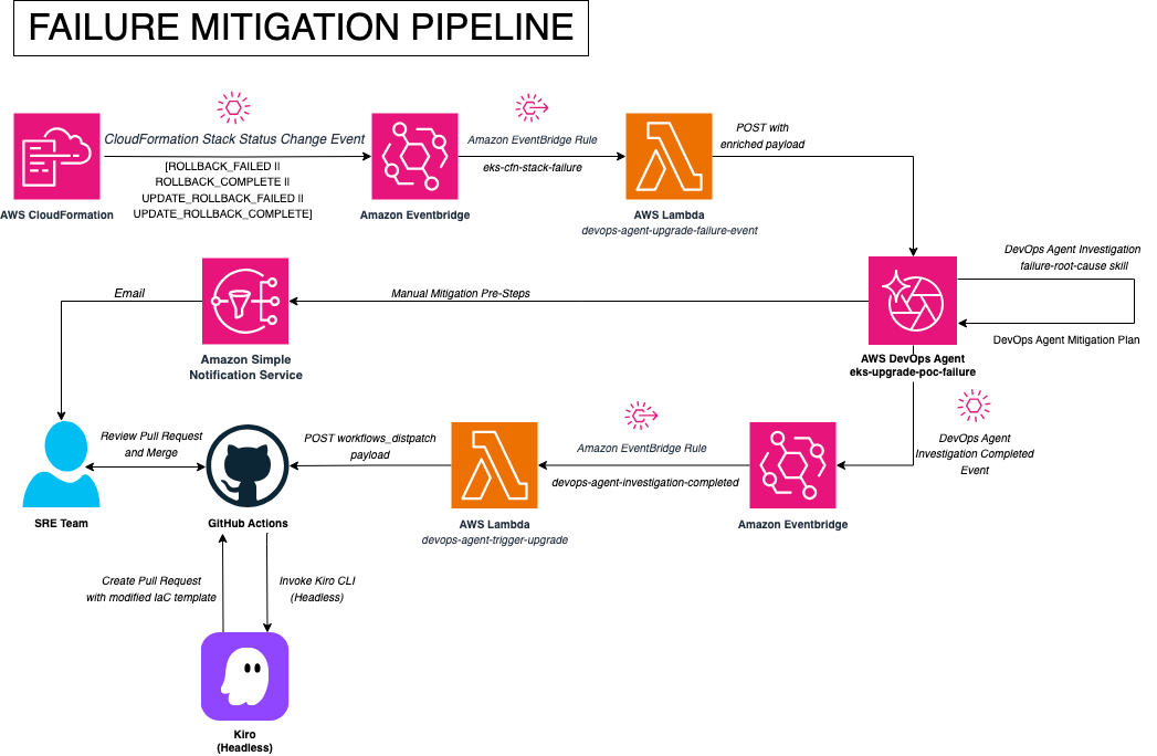
End-to-end Plan-Prove-Iterate workflow showing how AWS DevOps Agent orchestrates hypothesis generation, feature-flagged implementation, experimentation, guarded rollout, and outcome recording in a continuous improvement loop.
Each component has a distinct responsibility. AWS DevOps Agent orchestrates the cycle: it runs on a schedule as a Custom Agent which is a user-defined agent with its own instructions, skills, and connected tools that executes autonomously without pausing for input unless something fails. AWS DevOps Agent supports Custom Agents as a way to encode a specific workflow, including its decision logic, safety constraints, and cadence, into an agent that runs end-to-end on its own. In this solution, the Custom Agent reviews goals, generates hypotheses informed by prior outcomes, coordinates implementation and validation, and drives iteration across multiple experiment cycles.”. Kiro CLI runs in headless mode inside the Experiment MCP Server container on Amazon Bedrock AgentCore, implementing code changes behind LaunchDarkly feature flags and opening pull requests without a human operating an IDE.
LaunchDarkly hosts feature flags, experiments, and Guarded Releases, monitors metrics in real time, and reverts flag state when a threshold is breached. It also exposes a hosted MCP server with tools the agent calls directly. The Experiment MCP Server (custom, built for this solution) exposes the remaining operations over MCP: code implementation through Kiro, PR merge, and deployment triggering.
The agent acts as an MCP client connected to these two servers. LaunchDarkly’s hosted MCP server provides flag management, experiment lifecycle, Guarded Release, and observability tools. The Experiment MCP Server provides code implementation, PR merging, and deployment tools. This design separates decision-making from execution: the agent decides what to do, the MCP servers handle how.
Plan / Prove / Iterate
The lifecycle operates in three phases.
Plan — The agent decides the next action for a goal, generates a hypothesis informed by prior outcomes when iterating, and creates a feature flag in LaunchDarkly. It then invokes Kiro CLI to implement the change behind the flag and open a pull request. AWS DevOps Agent validates the change through release readiness review. After a green review, the PR is merged and a GitHub Actions workflow deploys the application through AWS Amplify.
Prove — Two sequential phases run after deployment. First, a 50/50 experiment splits 10% of traffic on a business KPI (for example, add-to-cart rate) until statistical significance selects a winning variation. Then a Guarded Release ramps the winning variation from 20% to 30% to 40% and eventually to 100% while LaunchDarkly monitors operational guardrails (error rate, page-load-time-p95). If a guardrail threshold is breached, LaunchDarkly reverts the flag state automatically, requiring no redeployment. The experiment measures value (does the change improve the goal metric?); the Guarded Release measures safety (does the change hold up at scale?).
Iterate — After a rollout concludes, the agent queries LaunchDarkly’s Change History API to associate specific flag modifications with outcomes. The recorded outcome informs the next hypothesis, and the cycle repeats until the goal is met or the agent recommends waiting.
Extending the agent with a custom MCP server
AWS DevOps Agent reads code, reviews changes, and decides what to do next. It does not take action on its own. To move from decision to execution, you connect it to MCP servers that expose operations as tools.
LaunchDarkly’s hosted MCP server covers flags, experiments, and Guarded Releases. We needed operations it doesn’t cover — writing code, merging PRs, and deploying — so we built the Experiment MCP Server. It runs on Amazon Bedrock AgentCore and exposes five tools: create_task and get_task_status (invoke Kiro CLI to implement changes and open a PR), merge_pr, trigger_deployment, and get_deployment_status.
These are mutation operations. When the agent calls create_task, Kiro writes real code. When it calls merge_pr, that code lands in main. You are responsible for this server — what it exposes, which repos it can touch, which branches it can merge to. We scoped ours to one repository, one branch, and one Amplify application. Those constraints live in the MCP server’s code, not the agent’s prompt, because API-level scoping cannot be misinterpreted.
The Experiment MCP Server [CG1] is a Python application built on FastMCP, packaged as a container and deployed to Amazon Bedrock AgentCore over stateless HTTP so the platform can restart or replace the container without breaking in-flight requests. At startup, the container pulls credentials from AWS Secrets Manager, clones the target repository, and makes Kiro CLI available as a local binary. This single-container design keeps everything colocated: when the agent calls create_task, the server spawns Kiro CLI as a headless subprocess with direct filesystem access to the cloned repo rather than making a network call to a separate code-generation service. Kiro CLI receives a structured prompt containing the task description, the LaunchDarkly flag key, and the variation details, then writes the change, commits to a new branch, and pushes. The server opens a pull request through the GitHub API and returns the task ID immediately without waiting for Kiro to finish. The caller polls get_task_status, which long-polls against an S3-backed state store so task progress survives container restarts. Deployment tracking follows a similar pattern: trigger_deployment dispatches a GitHub Actions workflow and returns the real GitHub run ID, and get_deployment_status reads live status directly from GitHub, so there is nothing to lose if the container cycles between calls. The overall design principle is that the MCP server coordinates work and delegates persistence to external systems (S3 for task state, GitHub for deployment state, Secrets Manager for credentials) rather than holding anything in memory that a restart would erase.
How the agent works
The agent runs on a schedule. Each run, it evaluates the current state of each goal and picks one of three actions: create a new experiment (no active rollout exists), iterate on a prior result (a rollout completed and the goal is not yet met), or wait (an experiment or rollout is still in progress).
The entry point for the system is an outcome, not a task list. The team picks a business metric from the available set — add-to-cart rate, checkout conversion, bounce rate, or page-load-time-p95 — and sets a target improvement, for example “increase add-to-cart rate by 10%.” Error rate is reserved as a safety guardrail during the Guarded Release phase and cannot be chosen as the primary success metric, because the system needs an independent operational signal to decide whether a winning variation is safe to scale. Beyond the metric and the target, all other inputs are optional. The agent infers the current baseline, the areas of the application in scope for changes, and any constraints from the codebase and production data. If those assumptions are off, the team corrects them before any code is written. The team states where they want to end up, and the agent works backward from there.
Demo Store product listing page used as the test surface for the add-to-cart experimentation cycles. Product cards currently show the control layout (no inline Add to Cart button).
For new goals, the agent explores the target repository and proposes a code change likely to move the metric. For iterations, it reads prior outcomes and adjusts its approach based on what worked and what did not. Before any code change, the agent creates a feature flag in LaunchDarkly (boolean, OFF by default, named with a convention like exp-add-to-cart-*) so every change ships behind a flag from the start.
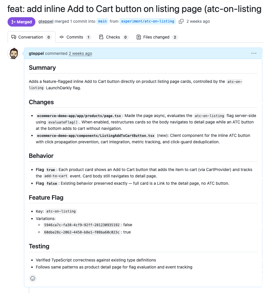
Implementation runs through Kiro CLI in headless mode. The agent calls create_task, Kiro clones the repository, writes the change behind the feature flag, and opens a pull request.
Merged GitHub PR implementing the feature-flagged inline Add to Cart button on the product listing page, controlled by the atc-on-listing LaunchDarkly flag.
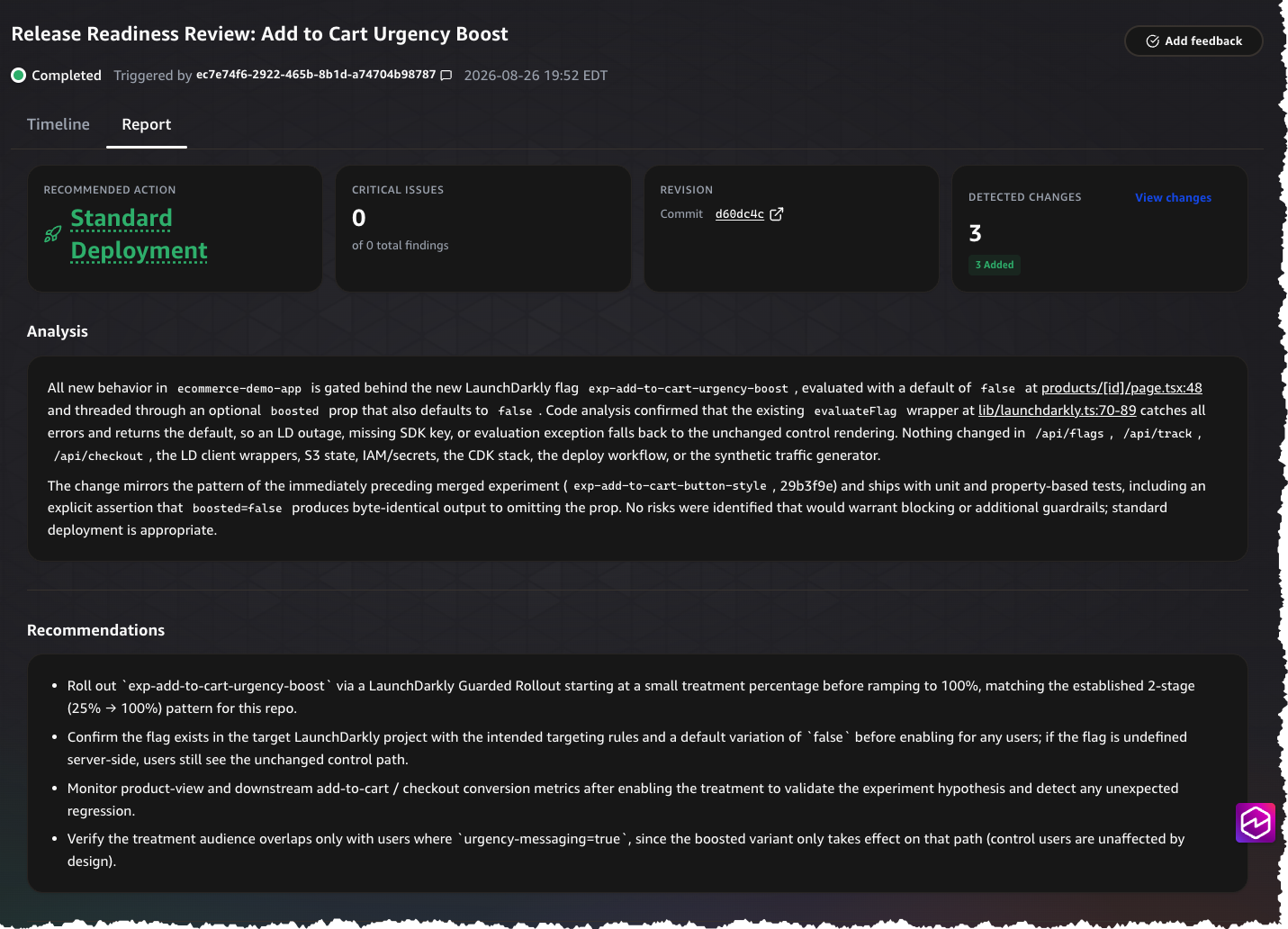
AWS DevOps Agent then runs a release readiness review on the PR. If the review fails, the agent retries up to three times before stopping to ask for help. After a green review, the PR is merged and a GitHub Actions workflow deploys through AWS Amplify.
AWS DevOps Agent Release Readiness Review for the Add to Cart Urgency Boost experiment. The automated review found zero critical issues and recommended standard deployment with a guarded rollout.
Proving the change
Once deployed, the flag is toggled on and the experiment begins. The agent creates a 50/50 experiment across 10% of traffic, splitting on the goal’s business KPI. In production, experiment data comes from real users interacting with your application, with metrics emitted through OpenTelemetry to LaunchDarkly. For this reference implementation, we built a synthetic traffic generator that simulates user sessions across both treatment and control variations, producing the conversion events and operational metrics that drive experiment decisions. It runs alongside the demo application and generates enough volume to reach statistical significance within minutes rather than days. The synthetic traffic generator is a demo convenience, not a production requirement. Any application that emits the right events to LaunchDarkly will work with this architecture.
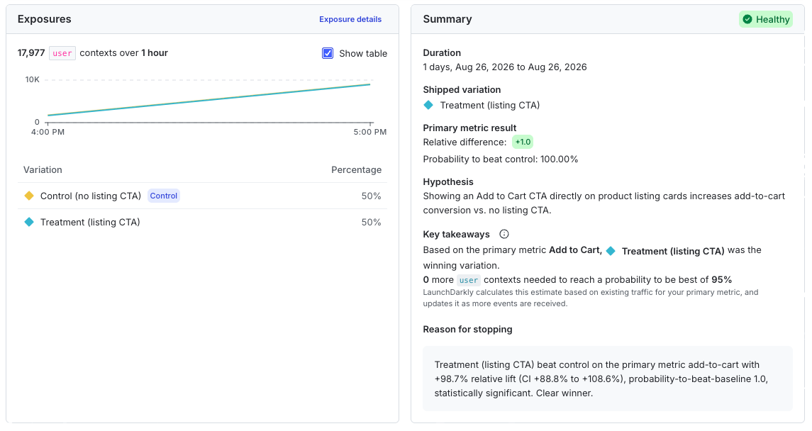
The agent checks for results on each Custom Agent execution until statistical significance is reached. In an interactive chat session, you prompt the agent to check when you are ready. If the treatment wins, the agent proceeds to the Guarded Release. If it loses, the agent archives the flag and records the outcome for the next iteration.
LaunchDarkly experiment summary for the inline Add to Cart listing CTA test. Treatment won decisively with 98.7% relative lift in add-to-cart conversion and 100% probability to beat control.
The Guarded Release ramps the winning variation from 20% to 30% to 40% while LaunchDarkly [1] applies sequential testing to the operational guardrail metric, halting the rollout as soon as the data shows a statistically significant regression against the original variation.. If a guardrail threshold is breached at any stage, LaunchDarkly reverts flag state at runtime without a redeployment. Guarded Releases and automatic rollback serve as the runtime safety net: if something goes wrong after deployment, the system reverts flag state without waiting for a human to intervene.
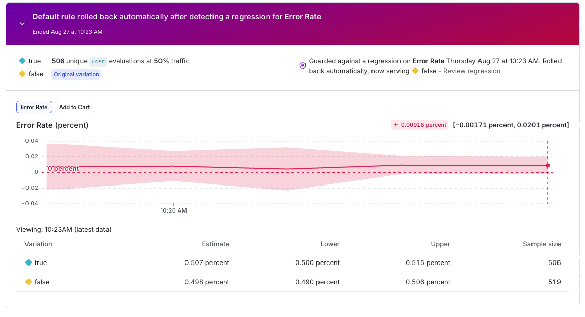
To validate the safety net in the reference implementation, we triggered a simulated error-rate spike during the ramp. LaunchDarkly detected the regression within the monitoring window, halted the rollout, and reverted the flag to its pre-rollout state automatically. No human intervened, no redeployment ran, and the application returned to the control behavior within seconds. The screenshot below shows the Guarded Release dashboard after the rollback.
LaunchDarkly Guarded Release auto-rollback event. The system detected an error rate regression during the ramp phase and automatically rolled traffic back to the control variation.
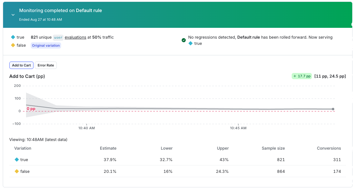
After recording the rollback and feeding the outcome into the next iteration, the agent adjusted its approach and proposed a revised implementation that avoided the latency regression. The second attempt followed the same pipeline: hypothesis, feature flag, implementation, review, deployment, experiment, and Guarded Release. This time, monitoring completed with no regressions detected. LaunchDarkly rolled the winning variation forward to full traffic, with add-to-cart conversion lifting from 20.1% to 37.9% across the treatment population, confirming the experiment result held at scale.
LaunchDarkly Guarded Release monitoring completion. The Add to Cart metric showed a 17.7 percentage point lift with no regressions, so the system graduated the treatment to 100% of traffic.
After each cycle, the agent generates a report documenting the hypothesis, experiment results, rollout outcome, and a recommendation for the next iteration. This report feeds into the next decision, so no context is lost between cycles.
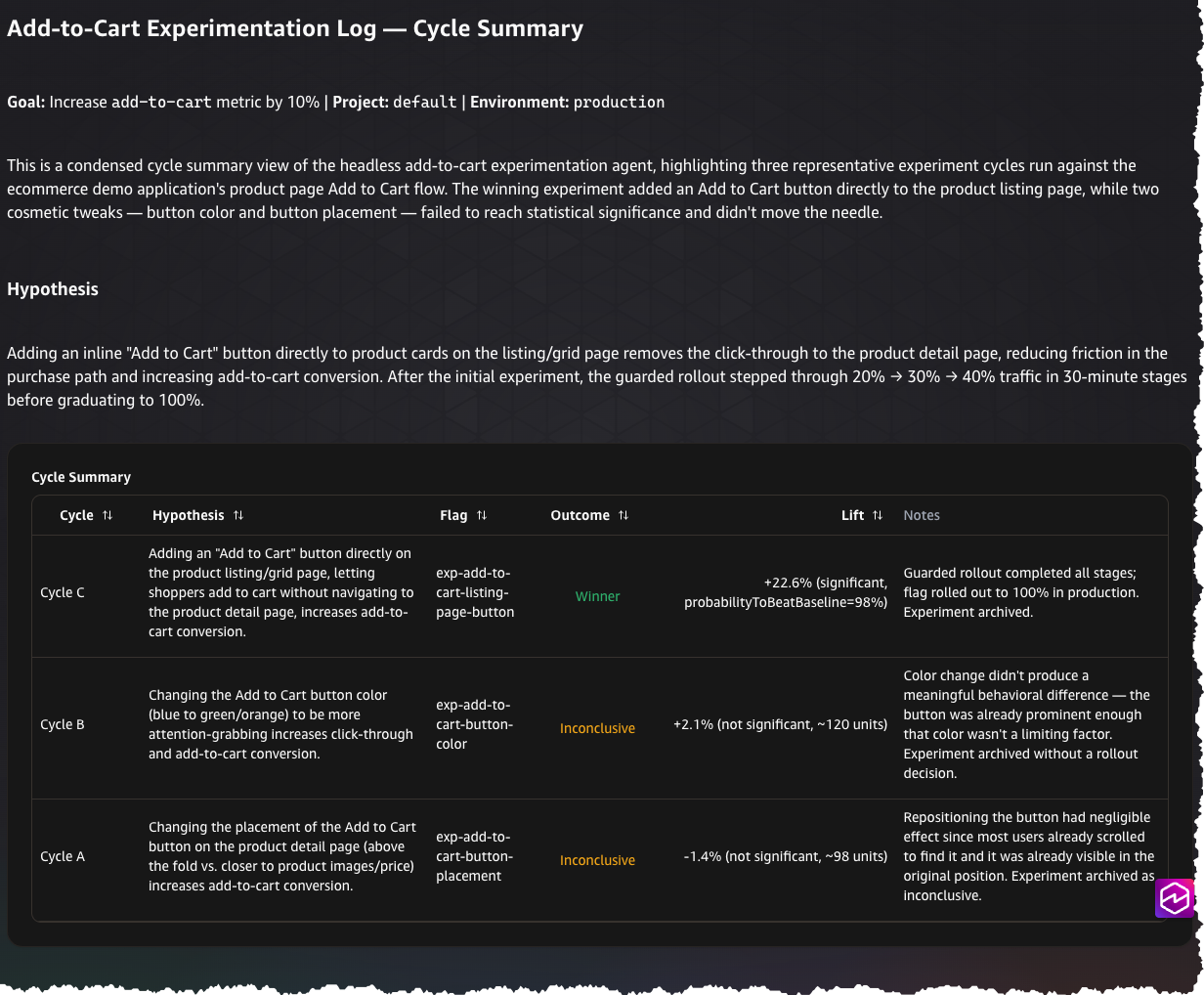
Experimentation cycle summary showing three hypothesis-test iterations. Only Cycle C (inline Add to Cart on listing page) reached statistical significance and was promoted to production. The two cosmetic experiments (button color and placement) were inconclusive.
Safety boundaries
The system operates within defined constraints. The agent validates every change through release readiness review before merge. It creates a feature flag before writing any code, so every change can be toggled off without a redeployment. Guarded Releases enforce operational guardrails at runtime with automatic rollback. The agent retries failed validations up to three times, then stops and asks for help rather than proceeding. All credentials are stored in AWS Secrets Manager and referenced by name only, never exposed in agent logs or tool calls.
Getting started
To implement this workflow, you need AWS DevOps Agent enabled in your AWS account, a LaunchDarkly account (start with a free 30-day AWS trial), and a target application and repository. The reference uses a Next.js app deployed through AWS Amplify. Experiments are available on every LaunchDarkly plan, including the free Developer plan. Guarded Releases, which automate progressive rollouts with automatic rollback, require a LaunchDarkly Enterprise plan with the Guardian add-on. Without Guarded Releases, the workflow still runs experiments and reports results. You manage the rollout manually instead. If your plan does not include Guarded Releases, update the agent skill definition below to remove the Guarded Release actions.
Setup requires three steps. First, add the LaunchDarkly remote MCP server to your AWS DevOps Agent space. Second, deploy the Experiment MCP Server container to an AgentCore runtime, storing API keys and tokens in AWS Secrets Manager. Third, create your custom agent with the orchestration skill. Use the experimentation skill in AWS DevOps Agent to guide you through defining goals, connecting the MCP servers, and writing the orchestration instructions. The full orchestration skill is included below.
---
name: "experiment-orchestration"
description: "Orchestrates automated experimentation lifecycle using LaunchDarkly Guarded Rollouts, an AI coding agent for implementation, and GitHub Actions for deployment."
---

# Automated Experimentation

Use this skill when you have a goal you want to move through experimentation (e.g., "increase checkout conversion by 15%", "decrease page load time by 20%").

**Core principle: experiment first, then guarded rollout.** Always prove a change on a small, fixed slice of traffic via an A/B experiment before ramping it up through a guarded rollout. Never start a guarded rollout blind — it exists only to scale a change the experiment has already shown to work.

**Execution mode:** once the goal is confirmed (Step 1), run Steps 2–8 end-to-end. Async operations (code implementation, release review, deployment, experiment monitoring, rollout monitoring) should be checked periodically, not tight-polled — see the waiting note in each step. Only stop and ask the user something if a step fails unrecoverably (repeated failed release reviews, deployment failure, or an inconclusive/losing experiment result).

**The final report (Step 8) is mandatory, not optional.** The moment an experiment or rollout reaches a terminal outcome — winner, loser, inconclusive, or rollback — produce the full report in the same turn you announce the outcome. Don't let a casual "it worked! ????" substitute for the structured report.

## Step 1: Goal Clarification

Before doing anything, get answers to:

1. **What metric measures success?** *(Required)* e.g. conversion rate, page load time, bounce rate. Reserve your error-rate metric as a safety guardrail — never use it as the primary success metric.
2. **What's the target improvement?** *(Required)* e.g. 15% increase, 200ms decrease.
3. **What's the current baseline?** *(Optional — infer from production metrics if not given)*
4. **What parts of the app are in scope?** *(Optional — infer from the codebase if not given)*
5. **Any constraints?** *(Optional)* e.g. no changes to the payment flow.

Questions 1–2 are required before proceeding; infer 3–5 where possible and confirm your assumptions with the user before implementing.

## Step 2: Hypothesis Generation

Explore the target repository/codebase to find a plausible change:

1. Search and read the relevant code paths.
2. Think through what UI/UX or logic change could plausibly move the chosen metric.
3. Check whether this hypothesis (or something close to it) has already been tried and failed — look at flag history or archived flags with similar naming. Avoid repeating a known failure.
4. Present the hypothesis to the user before proceeding, along with your reasoning and any inferred assumptions from Step 1.

**Before finalizing a flag key, check for collisions:** look up any candidate flag key first.
- Already fully shipped (100% one variation, no split) → already decided, pick a different hypothesis.
- Actively running an experiment → mid-flight, don't compete with it, pick a different hypothesis.
- Doesn't exist → safe to create.

## Step 3: Implementation

1. Create a boolean feature flag, OFF by default in all environments. Name it with a clear pattern like `exp-<metric>-<short-description>` (e.g. `exp-checkout-conversion-cta-color`), lowercase with hyphens, ~50 chars max.
2. Hand off implementation to your coding agent/tool of choice, with clear instructions to gate the change behind the exact flag key from step 1.
3. This step is asynchronous — check status periodically rather than looping tightly on it.
4. Once implementation completes, move to Step 4 with the resulting branch/PR. If it fails, report the error and stop.

## Step 4: Release Readiness

Run your standard release/risk review on the PR before merging.

- If it passes: merge the PR.
- If it fails: feed the review's specific feedback back into implementation and retry. Cap retries at a small fixed number (e.g. 3 attempts total) — if it still hasn't passed, stop and report the last failure to the user rather than retrying indefinitely.

*(If your environment genuinely has no review capability available — e.g., a fully unattended automation context — you can skip straight to merge, but treat that as a deliberate, narrow exception you call out explicitly, not a default. Skipping review removes your only gate against shipping broken code.)*

## Step 5: Deployment

Deployment typically won't fire automatically on merge if your workflow is manually-triggered (`workflow_dispatch`-only) — you'll need to trigger it explicitly.

1. Trigger the deploy workflow on the merge target branch. Treat "already an in-progress deployment for this ref" as expected de-duplication, not an error — don't re-trigger.
2. Poll for status, but let your polling tool's own internal long-poll do the waiting rather than looping tightly yourself.
3. Watch for a "stale" status specifically: if a deployment reports "running" for far longer than normal, cross-check the actual CI run history by commit SHA/timing before assuming it's still in progress — a background poll process may have died without updating the record.
4. **Trigger a deployment at most once per attempt.** If you're unsure whether a previous trigger succeeded, check status first — never re-trigger just because you're unsure.
5. On timeout: stop, check the CI run directly, report the situation, ask how to proceed.
6. On explicit failure: stop and report — do not proceed to the experiment.
7. On success: proceed immediately to Step 6.

## Step 6: Experiment Phase (fixed 10%)

Prove the change on a small, fixed slice of traffic. Do **not** start a guarded rollout here — that's Step 7, and only after this proves out.

1. Turn the flag ON.
2. Configure a fixed 50/50 split across 10% of traffic (a flat allocation, not a staged ramp) on your chosen randomization unit (typically "user"). The remaining 90% of traffic is excluded from the experiment entirely.
3. Create an experiment with:
   - Exactly one primary metric: the success metric from Step 1.
   - Guardrail metric(s): always include your error-rate metric; add a performance metric (e.g. p95 page load time) too if this is a performance-focused change.
   - Treatments: control (off) at 50%, treatment (on) at 50%, allocated to 10% of total traffic.
4. Start the experiment/data collection.
5. Move to Step 7 to monitor toward a decision.

## Step 7: Monitoring & Outcome

Check status periodically — don't tight-loop. In an interactive session, check once and report progress, then pick back up later. In an unattended/scheduled context, check once per invocation and persist your progress somewhere durable between runs.

**Phase 1 — Prove the experiment at 10% (gate before any rollout):**

Watch for statistical significance on the primary metric:

- **Significant + positive lift** → experiment proven. Stop the experiment iteration and move to Phase 2.
- **Significant + negative lift** → declare a loser, archive the flag, skip Phase 2, go straight to the Step 8 report.
- **No significance after a reasonable ceiling (e.g. 30 minutes)** → report "inconclusive, need more traffic" and stop; don't proceed to Phase 2.

Never declare a winner off a single data point or before your stats engine confirms significance.

**Phase 2 — Guarded rollout ramp (only after Phase 1 proves the change):**

Start a guarded rollout with:
- The winning ("on") variation as the test, the original as control.
- Same randomization unit as the experiment.
- **Exactly 3 monitored stages, capped well below 100%** — e.g. 20% → 30% → 40%, ~60 minutes monitoring each. Don't add a stage at or above 100%; Guarded-rollout implementations reject stages above 50% audience allocation, and the rollout auto-promotes to 100% itself once the final monitored stage completes cleanly — no explicit 100% stage needed.
- The same primary + guardrail metrics as the experiment, each configured to notify and auto-rollback on regression.

Track stage progression. If the rollout rolls back or stops at any point, treat it as a regression: declare failed, clean up the flag (deprecate/archive it), and go to the Step 8 report.

Once the final stage completes cleanly and auto-promotes to 100%, declare a winner and go to the Step 8 report.

**Retrying after a rollback:** a rollback isn't always caused by your monitored metrics genuinely regressing — it can also be triggered by an unrelated application error surfacing mid-ramp. Before blindly restarting after the user says they've fixed something:
1. Confirm the flag's current state (should be back to 100% control, nothing stuck mid-rollout).
2. Check the change history timing between "advanced to next stage" and "reverted." A rollback within seconds of advancing is inconsistent with a full metric-window regression and points to an external cause instead.
3. If the flag is cleanly reverted and the external cause is confirmed fixed, it's safe to restart the guarded rollout from scratch with the same parameters.
4. Don't silently retry without this check, and don't refuse to retry just because a prior attempt rolled back — a genuinely fixed external cause is a legitimate reason to retry. A metric-driven loser is not — don't retry that.

**On any terminal outcome, immediately produce the Step 8 report in the same turn** — a one-line "it worked!" note is fine as a lead-in, but the structured report must follow, not wait for a follow-up request.

## Step 8: Report

Runs automatically the instant Step 7 reaches a terminal outcome (winner + auto-promoted to 100%; loser; inconclusive; or rollback/failure). Use this exact structure:

```
## Experiment Report: [Goal Description]

**Date:** [YYYY-MM-DD]
**Goal:** [metric] [direction] by [target]%
**Status:** [achieved / in progress / stalled]

### Hypothesis
[What we tried and why]

### Implementation
- Flag: [flag_key]
- Files modified: [list]
- Branch: [branch name]

### Release Readiness
- [reviewed, passed after N attempt(s) / skipped, per your environment's process]

### Experiment Phase (10% fixed split)
- Status: [proven / loser / inconclusive]
- Duration: [time]
- Metric change: [before] → [after] ([+/-]%)
- Statistical significance: [value, confidence interval]

### Guarded Rollout Phase (if reached)
- Status: [completed / rolled_back / not started]
- Duration: [time]
- Stages reached: [N of 3 monitored stages]
- If rolled back and retried: [root cause, outcome of retry]

### Safety Metrics
- error-rate: [baseline] → [final] ([no regression / regression detected])
- [other guardrails]: [baseline] → [final] ([status])

### Next Steps
[What to do next based on the outcome]
```

## Safety Rules (the non-negotiables)

- Always present the hypothesis before implementing.
- Always run a release/risk review before merging, unless your environment has a deliberate, explicitly-called-out exception.
- **Always prove a change via a fixed small-percentage experiment before starting any guarded rollout** — never ramp blind.
- Always include an error-rate (or equivalent "don't break prod") metric as a guardrail, separate from your success metric.
- Add a performance guardrail (e.g. p95 latency) for performance-focused changes.
- Every rollout metric should be configured to both notify AND auto-rollback on regression — don't rely on notification alone.
- **Cap guarded rollout stages well below 100%** (most platforms reject stages ≥50% audience allocation) and let the platform auto-promote to 100% after the final stage — don't try to add an explicit 100% stage.
- Distinguish a metric-driven rollback (don't retry) from an external-cause rollback (safe to retry once fixed) before restarting a rolled-back rollout.
- The final report is automatic and mandatory on every terminal outcome — never defer it to a follow-up ask.
Conclusion
This post described how AWS DevOps Agent, Kiro CLI, and LaunchDarkly connect into a closed-loop system that turns an improvement goal into a series of measured, safe experiments. The agent runs autonomously on a schedule: it generates hypotheses informed by prior outcomes, creates feature flags before any code change, invokes Kiro CLI in headless mode to implement changes behind those flags, validates through release readiness review, deploys through GitHub Actions and AWS Amplify, and hands off to LaunchDarkly for experiment measurement and guarded rollout. If a guardrail is breached at any point during the rollout, LaunchDarkly reverts flag state at runtime without a redeployment. After each cycle, the agent records what happened and feeds it into the next decision.
This directly addresses the three barriers that slow experimentation:
● Planning cost is reduced because the agent handles hypothesis generation, flag creation, implementation coordination, and validation. The team defines the goal; the system handles the wiring.
● Measurement disconnected from action is addressed because LaunchDarkly monitors metrics in real time and reverts flag state automatically when a guardrail is breached, requiring no redeployment and no waiting for a human to notice.
● Stalled iteration is solved because every outcome is recorded and fed into the next hypothesis automatically. The system does not forget what it learned, and it does not stall between iterations.
The architecture is available to implement today as a reference. The orchestration skill included in this post encodes the full 8-step workflow: goal clarification, hypothesis generation, implementation, release readiness, deployment, experiment, monitoring, guarded rollout, and reporting. Teams define their improvement goal, connect the LaunchDarkly MCP server and the Experiment MCP Server to a DevOps Agent custom agent, and let the system iterate toward the target within the safety boundaries they configure. A more turnkey experience is planned for the future.
Не мога да спя и мисля глупости, и се ядосавам, щото someone is wrong on the internet. Тия дни четох нещо много полезно по темата за “това е просто инструмент”, и имам малко мисли по темата (писанието е доста по-добро от моето, ама имам нужда и аз да напиша нещо).
Първо, това е thought-terminating cliche – хората го казват като приключващо спора, колкото и глупаво и малоумно да е. Нито един инструмент не е “просто” инструмент – всеки инструмент носи със себе си допълнителни последствия, и има ефекти в/у нас и светът около нас, колкото и да си затваряме очите.
Преди да стигна до текущия “просто инструмент”, мога да дам няколко супер очевидни примера за “просто инструменти”, които имат много по-голямо влияние от базовата си функция.
Колите са един такъв прост и очевиден пример – основната им функция е транспортна, но на практика имат огромно влияние върху здравето (замърсяване и катастрофи), архитектурата на градовете, сегрегацията (в щатите са я докарали до наука, как да държим по-тъмнозелените надалеч, като направим така, че за тях няма транспорт), и т.н., и т.н..
Друг прост пример са оръжията и парите, които са различно регулирани на различни места. И за двете има политически течения, дето твърдят, че това са просто инструменти, но да отречем тяхното огромно влияние би било чак смешно.
И сега имаме някакви нови неща. Например, интернетът навсякъде, който също има огромно влияние. И който също е просто инструмент, който обаче с малко добавки почна да има сериозна роля в резултатите от различни избори по света, като един от по-крайните ефекти. После, bitcoin и подобните валути, които много улесниха прането на пари и разни незаконни разплащания, както и дадоха нов живот на стари схеми за измама. И сега AI, което за всичкия ток, който харчи, върши смислена работа на сравнително малко хора (не броя тия, дето усилено работят да издоят всичките пари на тоя свят, само за потребителите му), но се промотира като наследник на нарязания хляб и топлата вода.
Та, следващия, който тръгне да ми обяснява за как AI (или каквото и да е) е “просто инструмент”, ще му обясня, че и псуването на майка е просто инструмент и това, че го пращам да се съвокуплява с нея си е част от инструмента и няма що да се ядосва. В крайна сметка, той и хероинът е едно просто обезболяващо, къде ни е проблема…
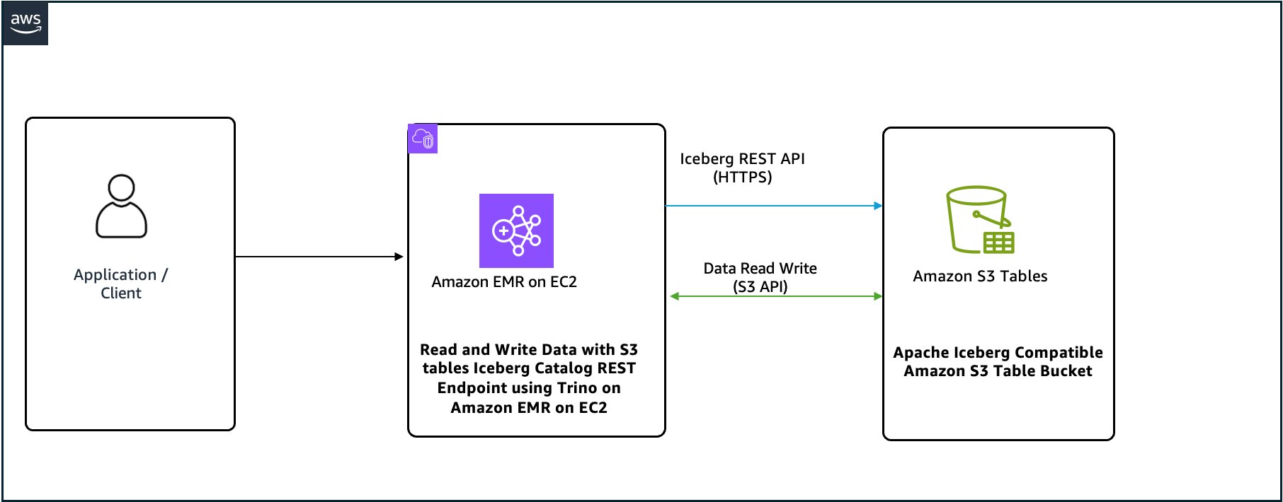
Organizations running analytics on Amazon Simple Storage Service (Amazon S3) data lakes often struggle with the operational overhead of managing Apache Iceberg tables, including compaction, snapshot expiration, and metadata tracking, while still needing fast, interactive SQL access across large volumes of data. Amazon S3 Tables, a capability of Amazon S3, addresses this by providing a purpose-built storage layer with native Apache Iceberg support and automated table maintenance. When you query S3 Tables from Amazon EMR using Trino and the Iceberg REST endpoint, you get a fully managed, open-standards-based analytics stack without the undifferentiated heavy lifting of table upkeep.
When paired with Amazon EMR running Trino, organizations gain access to a high-performance distributed SQL query engine capable of processing large-scale datasets. Trino’s ability to query data across multiple sources, combined with the automated optimization features of S3 Tables, creates a flexible analytics platform. The integration uses Apache Iceberg’s REST catalog specification, providing a standardized interface that supports compatibility across different compute engines while maintaining full control over query execution and data processing logic.
This architectural pattern is particularly valuable for organizations seeking to modernize their data platforms without vendor lock-in, as it relies on open standards and formats. The solution delivers high-throughput query performance with distributed SQL execution while significantly reducing the operational burden of managing table metadata, compaction, and snapshot lifecycle management. In this post, we show you how to create and query Amazon S3 Tables using Trino on Amazon EMR through the Apache Iceberg REST catalog endpoint.
Solution overview
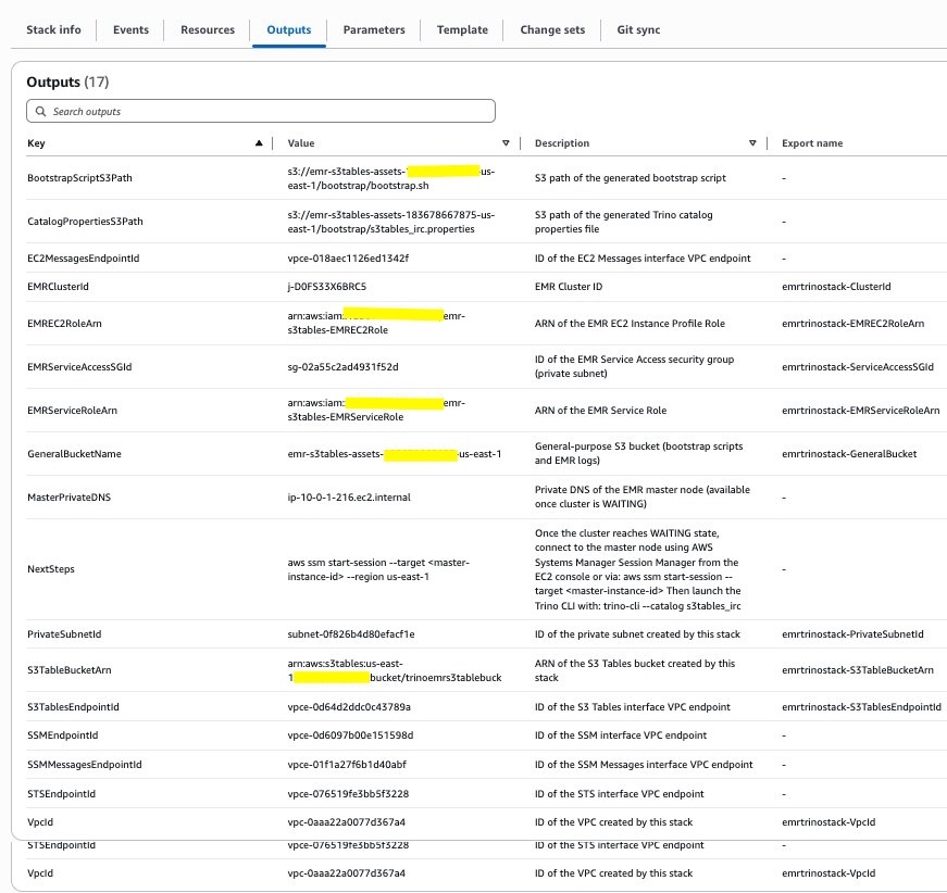
This implementation demonstrates a complete integration between the Trino distribution on Amazon EMR and Amazon S3 Tables through the Apache Iceberg REST catalog endpoint. The architecture uses several key AWS services working in concert:
Amazon EMR serves as the managed compute layer, providing a scalable Hadoop framework that hosts the Trino query engine. Amazon EMR handles cluster provisioning, configuration management, and automatic scaling, allowing teams to focus on analytics rather than infrastructure management.
Apache Trino acts as the distributed SQL query engine, offering ANSI SQL compatibility and the ability to process queries across massive datasets with low latency for interactive workloads. Its connector architecture supports integration with various data sources, including the Iceberg REST catalog.
Amazon S3 Tables provides the storage and catalog layer, managing Apache Iceberg tables with built-in optimization. The service automatically handles compaction, snapshot expiration, and metadata management, reducing operational overhead while maintaining query performance. S3 Tables exposes a REST API endpoint that conforms to the Apache Iceberg REST catalog specification, which provides standardized integration with any Iceberg-compatible engine.
Apache Iceberg REST endpoint serves as the communication protocol between Trino and S3 Tables. This RESTful interface handles catalog operations including namespace management, table creation, metadata retrieval, and transaction coordination. The endpoint supports AWS Signature Version 4 authentication for secure access to table resources.
The data flow follows this pattern: Users submit SQL queries through the Trino CLI or JDBC interface. Trino’s Iceberg connector communicates with the S3 Tables REST endpoint to retrieve table metadata and plan query execution. The query engine then reads data directly from S3 using optimized file formats (Parquet, ORC) while using Iceberg’s metadata layer for partition pruning and predicate pushdown. Write operations follow a similar path, with Trino coordinating with S3 Tables to commit new data files and update table metadata atomically.
This architecture delivers several key benefits: separation of compute and storage for independent scaling, automated table maintenance reducing operational costs, open-source format compatibility preventing vendor lock-in, and fine-grained access control through AWS Identity and Access Management (IAM) and AWS Lake Formation integration.
Figure 1: Solution architecture for querying Amazon S3 Tables from Trino on Amazon EMR
Prerequisites
Before getting started, make sure that you have the following:
An active AWS account with billing enabled.
An AWS Identity and Access Management (IAM) user with specific permissions to create and manage resources, such as a virtual private cloud (VPC), subnet, security group, IAM roles, Amazon EMR, Interface VPC endpoints, S3 Tables bucket and S3 buckets.
Sufficient VPC capacity in your chosen AWS Region.
For this post, we create the solution resources in the US East (N. Virginia) Region (us-east-1) using AWS CloudFormation templates. In the following sections, we show you how to configure your resources and implement the solution.
Note: Querying Amazon S3 Tables through Trino on Amazon EMR requires Trino version 475 or later, available in Amazon EMR 7.11 and later.
Part A: Configure Amazon S3 Tables integration with Trino on Amazon EMR using AWS CloudFormation
In this post, you use the CloudFormation template emr-trino-s3tables.yaml.
This template deploys the following resources: a VPC with one private subnet, an S3 Tables interface VPC endpoint for private access, and an Amazon EMR cluster running Trino integrated with Amazon S3 Tables through the Apache Iceberg REST catalog endpoint.
It also creates an S3 Tables bucket, a general-purpose S3 bucket, IAM roles, and security groups.
At deploy time, it dynamically generates the Trino catalog configuration and bootstrap script.
To create the solution resources, complete the following steps:
Launch the stack emr-trino-s3tables.yaml using the CloudFormation template.
Provide the parameter values as listed in the following table.
Parameters
Description
Sample value
Stack Name
Name of CloudFormation stack
emr-s3tables-trino
VPC CIDR block
IP range (CIDR notation) for this VPC.
10.0.0.0/16
Private Subnet CIDR block
IP range (CIDR notation) for the private subnet in the second Availability Zone.
10.0.1.0/24
Resource name Prefix
Short prefix applied to every resource name
emr-s3tables
S3 Tables bucket name
Name of S3 table Bucket
trinoemrs3tablebuck
EMR release
Release version of Amazon EMR
EMR 7.12
The stack creation process can take approximately 15 minutes to complete. You can check the Outputs tab for the stack after the stack is created, as shown in the following screenshot.
Figure 3: CloudFormation stack outputs
Figure 3: CloudFormation stack outputs
Understanding the deployment
The CloudFormation template performs several key tasks:
Infrastructure provisioning: Sets up the Amazon EMR cluster with Trino, VPC, subnet, security group, and S3 table bucket.
Integration configuration: Sets up the Iceberg REST connector for S3 Tables.
Part B: Connecting Trino to Amazon S3 Tables with Iceberg REST endpoint
The CloudFormation template automatically configures the S3 Tables catalog in Trino on Amazon EMR. In the next section, we examine the configuration that drives this integration.
1. Catalog configuration details
A catalog in Trino on Amazon EMR is the configuration that grants access to a specific data source. Each Trino on Amazon EMR cluster can have multiple catalogs configured, allowing access to different data sources simultaneously.
As part of this setup, the CloudFormation template creates a catalog properties file at /etc/trino/conf/catalog/s3tables_irc.properties with the following configuration:
The following table lists the key properties in the catalog configuration on Trino:
Property name
Description
iceberg.rest-catalog.uri
REST server API endpoint URI (necessary).
iceberg.rest-catalog.warehouse
Warehouse ID or location for the catalog (necessary). For S3 Tables, this is the ARN for the S3 table bucket as shown in the preceding properties example.
iceberg.rest-catalog.sigv4-enabled
Must be set to ‘true’ (necessary)
iceberg.rest-catalog.signing-name
Must be set to ‘s3tables’ (necessary)
iceberg.rest-catalog.view-endpoints-enabled
Must be set to ‘false’ (necessary)
fs.hadoop.enabled
Must be set to ‘false’
fs.native-s3.enabled
Must be set to ‘true’
s3.iam-role
Amazon Resource Name (ARN) of the IAM role with permissions to S3 Tables. In this post, we use the same role, which is the service role for Amazon EMR.
s3.region
AWS Region, for example us-east-1
This configuration establishes a connection between Trino and the S3 Tables REST endpoint. You can have multiple catalogs registered, one per S3 table bucket, which is determined by the iceberg.rest-catalog.warehouse property.
3. Configure Amazon EMR service IAM role trust relationships
The Amazon EMR service role requires proper trust relationships to function correctly. Navigate to the IAM console and configure the trust policy for your Amazon EMR service role:
This trust policy establishes two critical relationships:
The Amazon EMR service can assume the role to manage cluster operations.
The EC2 instance profile can assume the role to access S3 Tables with elevated permissions.
4. Working with S3 Tables in Trino on Amazon EMR
Now that you have Trino on Amazon EMR set up and configured to work with S3 Tables, you can explore how to work with this integration.
4.1. Connecting to Trino on Amazon EMR
Navigate to Amazon EMR and select Connect to the primary node using AWS Systems Manager Session Manager for passwordless SSH.
Figure 4: Connecting to the primary node with Session Manager
When you’re connected, you can use the Trino CLI with your S3 Tables catalog:
sudo su - hadoop
trino-cli --catalog s3tables_irc
This connects you to the Trino on Amazon EMR using the S3 Tables integration you configured.
Figure 5: Trino CLI connected to the S3 Tables catalog
4.2. Examples: Creating and querying tables
In this section you run through some example queries to demonstrate the functionality.
4.2.1 Creating a namespace
First, you create a namespace (schema) in S3 Tables. A namespace in S3 Tables is a logical container or organizational unit that helps group related tables and objects together.
CREATE SCHEMA blog_namespace;
USE blog_namespace;
4.2.2 Creating a table
Create a table with various data types. You don’t need to specify the table type as Iceberg explicitly because you’re connecting to the Iceberg catalog. You can use all standard Iceberg capabilities, such as partitioning and sorting. Furthermore, some of the important Iceberg table properties that support table maintenance operations are configured with default values. You also have the option to edit the configurations using S3 Tables maintenance APIs.
CREATE TABLE IF NOT EXISTS customers (
customer_sk INT,
customer_id VARCHAR,
salutation VARCHAR,
first_name VARCHAR,
last_name VARCHAR,
preferred_cust_flag VARCHAR,
birth_day INT,
birth_month INT,
birth_year INT,
birth_country VARCHAR,
login VARCHAR
) WITH (
format = 'PARQUET',
sorted_by = ARRAY['customer_id']
);
Table property explanation:
format = 'PARQUET': Specifies Parquet as the file format for optimal compression and query performance.
sorted_by = ARRAY['customer_id']: Defines sort order within data files, improving query performance for customer_id filters.
Verify the table creation:
SHOW TABLES;
You should see customers in the output, confirming the table exists in the S3 Tables catalog.
4.2.3 Inserting data
You can insert some sample data into your table. You can also use an existing table in any of the catalogs configured in Trino on Amazon EMR to read data and write into the S3 table with an INSERT INTO ... SELECT statement.
This INSERT operation demonstrates Trino’s ability to write data to S3 Tables. Behind the scenes, Trino:
Writes data files in Parquet format to S3.
Communicates with the S3 Tables REST endpoint to register the new files.
Atomically commits the transaction, updating table metadata.
4.2.4 Querying data
Execute a SELECT query to retrieve and verify the inserted data:
SELECT * FROM customers LIMIT 10;
The query should return all eight customer records with proper formatting. You can also execute more complex analytical queries:
-- Count customers by country
SELECT birth_country, COUNT(*) as customer_count
FROM customers
GROUP BY birth_country
ORDER BY customer_count DESC;

-- Find customers born after 1990
SELECT first_name, last_name, birth_year
FROM customers
WHERE birth_year > 1990
ORDER BY birth_year;
These queries demonstrate Trino’s SQL capabilities and the integration with S3 Tables for both read and write operations.
4.3 Explore advanced features
S3 Tables with Iceberg provides several features for data management:
4.3.1 Time travel queries
Step 1: Check available snapshots.
-- Query table as of a specific timestamp. Check available snapshots
SELECT * FROM "customers$snapshots";
Step 2: Query the table as of a specific snapshot.
SELECT * FROM customers FOR VERSION AS OF <snapshot_id_from_step1>;
4.3.2 Schema evolution
-- Add a new column
ALTER TABLE customers ADD COLUMN email VARCHAR;

-- Rename a column
ALTER TABLE customers RENAME COLUMN login TO username;
Cleaning up
To clean up the resources, navigate to CloudFormation and delete the stack that you created.
Conclusion
This solution demonstrates an integration between Amazon EMR Trino and Amazon S3 Tables using the Apache Iceberg REST catalog specification. In this post, we showed you how to create and query S3 Tables from Trino on Amazon EMR. The architecture delivers several advantages for modern data platforms:
Operational simplicity: S3 Tables eliminates the complexity of managing Iceberg table metadata, compaction schedules, and snapshot lifecycle policies. The service handles these operations automatically, allowing data teams to focus on analytics rather than infrastructure maintenance.
Performance at scale: The architecture is designed for large-scale workloads. Trino distributes query execution across the cluster while Iceberg’s metadata layer helps the engine locate only the relevant data files. Features like partition pruning, predicate pushdown, and columnar file formats can help improve performance for both interactive and batch workloads.
Cost efficiency: This architecture separates compute and storage, so you can scale each independently based on workload requirements. S3 Tables automatically compacts small files to help reduce storage overhead, and Amazon EMR clusters can scale dynamically so you pay for compute only when needed.
Open standards and portability: By using Apache Iceberg’s open table format and REST catalog specification, this solution avoids vendor lock-in. Other Iceberg-compatible engines can access tables created in S3 Tables including Apache Spark, Apache Flink, and Dremio, providing flexibility in tool selection.
Fine-grained access control: Integration with IAM and resource-based policies provides access control at the table bucket, namespace, and table level. For fine-grained access at the column and row level, you can integrate with AWS Lake Formation. AWS Signature Version 4 authentication supports secure communication between Trino and S3 Tables.
ACID transactions: Iceberg’s transaction model guarantees atomicity, consistency, isolation, and durability for all table operations. This supports reliable concurrent reads and writes, making the platform suitable for production workloads requiring data consistency.
This architectural pattern is particularly well-suited for organizations building modern data lakehouses, migrating from traditional data warehouses, or consolidating multiple analytics platforms. The combination of the managed compute of Amazon EMR, Trino’s versatile query engine, and the automated table management of S3 Tables creates a strong foundation for data-driven decision making.
To learn more about the services and features discussed in this post, see the following resources:
AWS uses Planned Lifecycle Events (PLEs) for AWS Health to signal that a managed service version is approaching end of standard support. Several AWS services such as Amazon Elastic Kubernetes Service (Amazon EKS), Amazon Relational Database Service (Amazon RDS), Amazon OpenSearch Service, and Amazon ElastiCache publish these events through AWS Health when a running resource needs to move to a newer version before a published deadline. For the team receiving that alert, the work that follows is remarkably similar regardless of which service triggered it. Engineers must identify every affected resource across accounts and AWS Regions, determine the correct target version, and assess compatibility constraints for dependencies and consumers. They then update infrastructure-as-code (IaC) definitions to reflect the new versions, validate that no breaking changes are introduced, and deploy within the deadline. When multiple services reach end-of-support on overlapping timelines, each with dozens of affected resources, this per-service effort compounds into a sustained operational burden for engineering and operations teams.
AWS DevOps Agent is a frontier agent that resolves and proactively helps prevent incidents, continuously improving reliability and performance of applications on AWS and hybrid environments. AWS DevOps Agent helps review software changes for production risks while investigating incidents and identifying operational improvements as an experienced DevOps engineer.
AWS DevOps Agent and Kiro are transforming how organizations manage version upgrades across AWS managed services and turn these into a governed, event-driven workflow. The AWS DevOps Agent automates the investigation: it discovers impacted resources, analyzes upgrade paths, and produces a structured change specification. Kiro provides the agentic development environment to apply those changes, validate safety constraints, and open a pull request (PR) for human review. The engineer’s role shifts from executing the upgrade to reviewing a PR that has already been investigated, coded, and validated. The engineers can even write the upgrade logic as a custom AWS DevOps Agent skill, and the framework handles orchestration, validation, and delivery.
This post and the sample code demonstrates the approach with an end-to-end Amazon EKS upgrade example. The underlying pattern of event detection, agent-driven investigation, automated code changes, and a failure retry loop applies to other AWS managed services that publish AWS Health PLEs.
In this post, you will learn how to:
Automate planned lifecycle upgrade events detection using AWS Health and Amazon EventBridge
Use AWS DevOps Agent to investigate the upgrade path and produce a structured change spec.
Run Kiro CLI (headless mode) in a continuous integration and continuous delivery (CI/CD) pipeline to apply code changes, validate safety constraints, and open a pull request.
Close the loop with automatic upgrade deployment failure detection where a failed deployment triggers root-cause analysis, mitigation planning, operator notification, and a code fix pull request without human initiation.
Solution overview
The following diagram shows the end-to-end flow, from the initial AWS Health event through to the pull request and the pipeline upgrade loop.
Figure 1: Architecture diagram of the automated upgrade pipeline
There are five main phases in this flow. Let’s walk through each phase.
Phase 1: Detection
a. The pipeline starts when AWS Health publishes an AWS_EKS_PLANNED_LIFECYCLE_EVENT to the default Amazon EventBridge bus with the following event details:
service: EKS
eventTypeCategory: scheduledChange
eventTypeCode: AWS_EKS_PLANNED_LIFECYCLE_EVENT
affectedEntities: <array of cluster ARNs with status: PENDING>
eventRegion: <region of the affected cluster>
b. An Amazon EventBridge rule named eks-health-planned-lifecycle matches this event and invokes the AWS Lambda function devops-agent-health-event.
c. The Lambda function extracts the relevant information (cluster name and region), builds a webhook payload with eventType: incident and priority: HIGH, and POSTs to AWS DevOps Agent webhook endpoint, instructing the agent to follow the eks-upgrade-planning skill for the specific cluster and region. The Lambda function does not validate those values, so a failed extraction can leave the investigation running against placeholder data.
Phase 2: Investigation
a. AWS DevOps Agent uses the eks-upgrade-planning skill to discover cluster topology, validate the version increment, check addon compatibility, scan for deprecated APIs, and determine upgrade sequence.
b. The agent outputs a structured AWS Cloud Development Kit (AWS CDK) Change Spec containing target version strings for every component, a rollback readiness assessment (confirming the 7-day rollback window will be available post-upgrade), a feasibility assessment (READY, BLOCKED, or NEEDS_REMEDIATION), and a risk rating.
c. When AWS DevOps Agent completes its investigation, it emits an Investigation Completed event to Amazon EventBridge with the following event details:
a. A second Amazon EventBridge rule devops-agent-investigation-events matches this event, filtered by agent_space_id so that only events from the specific agent space trigger the pipeline.
b. The rule invokes the Trigger Upgrade Lambda function (devops-agent-trigger-upgrade). This Lambda function fetches the investigation’s journal records through ListJournalRecords and scans the output for content markers to determine the next action. Markers are checked in a fixed priority order so that a failure investigation quoting upstream CLUSTER_VERSION context cannot accidentally re-trigger an upgrade workflow. When either a CDK Change Spec heading or a resolved CLUSTER_VERSION line is present, the Lambda function treats the investigation as having produced an actionable upgrade plan. It retrieves the GitHub Personal Access Token (PAT) from AWS Secrets Manager, builds the investigation metadata into a summary JSON, and dispatches the eks-upgrade.ymlGitHub Actions workflow through the GitHub API. The dispatched payload is a compact summary record (~3.8 KB) containing the CDK Change Spec, not the full investigation transcript, which exceeds GitHub’s workflow dispatch size limit.
c. Before the workflow lets a coding agent near the code, it validates what the investigation produced. An extraction step scans the received payload for fenced code blocks containing CLUSTER_VERSION. Each candidate block is held to a strict format contract:
No leftover placeholder markers.
A Kubernetes version matching X.Y.
A kubectl layer package matching @aws-cdk/lambda-layer-kubectl-vNN.
Every addon version matching vX.Y.Z-eksbuild.N unless explicitly marked NOT_INSTALLED.
The workflow also enforces the agent’s own feasibility verdict. If the investigation concluded BLOCKED or NEEDS_REMEDIATION, the run stops and the coding agent is not invoked. When validation passes, the single deduplicated spec block is written to a temporary file for the coding step. The workflow stops with an error if no spec block is found, no block passes validation, or multiple conflicting specs are present. The pipeline fails closed rather than handing an ambiguous instruction to a coding agent.
d. GitHub Actions then installs Kiro CLI, gated on a minimum tested version, with anything newer allowed through but flagged as untested. The installer is downloaded and executed as two discrete steps rather than piped from curl, and Kiro is then invoked in headless mode:
kiro-cli chat --no-interactive --trust-tools=read,write,glob,grep \
"Read kiro-cdk-instructions.md for context on the CDK patterns. Then read /tmp/cdk-change-spec.txt — it contains the validated CDK Change Spec extracted from the DevOps Agent investigation. Apply those values exactly. Modify lib/iteration3-stack.ts ONLY. Do NOT derive or guess version numbers — use only the values from the spec file. Make only the file edits — do not run any build or shell commands, and do not commit."
e. Two things are worth noting about this invocation. Kiro is trusted with file tools only (read, write, glob, grep) with no shell or command execution, so the scope of the agent step is limited to file edits in the checked-out working tree. And it is told explicitly not to derive version numbers: every value comes from the validated spec file, so a model that misreads the investigation cannot substitute a version of its own. Kiro reads kiro-cdk-instructions.md, a standalone reference that prescribes the CDK modification procedure for EKS upgrades, then modifies lib/iteration3-stack.ts and nothing else. The kubectl layer dependency is handled separately, by npm, in a later step. Neither the AWS DevOps Agent nor Kiro can query a package registry, so neither can know which versions of that layer actually exist. The spec carries only the package name and npm resolves the version. It is the pipeline’s own principle applied to itself: identify what the model cannot know, and move it out of the model’s reach rather than letting it guess.
f. Two independent gates run after Kiro exits. The first diffs the working tree against a single-file allowlist and fails the run if anything other than lib/iteration3-stack.ts was touched. That diff is a containment check on the agent’s write access and only after that audit passes, a separate step updates the kubectl layer dependency in package.json. The second gate runs the full build and CDK synthesis pipeline, so a change that does not compile or synthesize does not create a pull request.
Phase 4: Review and deploy
a. After Kiro exits, the workflow opens a GitHub Pull Request (PR) on a branch named upgrade/eks-automated-<run_id>. Kiro’s role ends at file edits. It does not interact with Git or GitHub. The PR body includes a rollback window advisory documenting the 7-day reversal deadline, a reviewer checklist, and a machine-readable investigation-context block containing the agent space ID and task ID. The post-merge deploy workflow parses that block to tag the AWS CloudFormation stack, so a future upgrade failure carries a record of which investigation produced the deployed plan. The tag is informational only and the failure investigation is not linked to the upgrade investigation, keeping the two workstreams independent.
b. The automated pipeline pauses at the pull request. The Site Reliability Engineering (SRE) team reviews the changes using their existing approval process.
c. After merge, the team deploys using their standard CI/CD pipeline. The investigation-context tags on the stack enable traceability back to the originating event if issues arise.
Phase 5: Failure detection and automated mitigation
The pipeline includes a closed-loop failure path. If a deployed upgrade fails, the system automatically investigates the root cause, generates a mitigation plan, notifies the SRE team, and opens a code fix pull request, all without human initiation. The pipeline attempts this automated recovery once. If the failure investigation itself does not produce actionable results, the pipeline stops and we recommend manually reviewing the cluster upgrade failure through the AWS DevOps Agent console or standard operational runbooks.
With EKS version rollbacks now available, the eks-failure-root-cause skill evaluates whether a rollback is the faster recovery before recommending a code fix. In case a deployment failure occurs within the 7-day rollback window, the root-cause investigation first evaluates whether a version rollback would resolve the issue faster than a code fix. When rollback readiness checks pass and the root cause is version-related (not a code or configuration error), the skill directs the agent to recommend version rollback (aws eks update-cluster-version --kubernetes-version <previous-version>) as the primary recovery action, with the code fix PR as a follow-up hardening measure. If rollback is not viable (outside the window, node skew, forward-only addon changes), the pipeline continues to the existing code fix workflow.
The following diagram shows the failure path from CloudFormation rollback through to the code fix pull request and operator notification.
Figure 2: Architecture diagram of the failure mitigation loop
a. When cdk deploy fails after merge, CloudFormation emits a stack status change event (such as ROLLBACK_FAILED, ROLLBACK_COMPLETE, UPDATE_ROLLBACK_FAILED, or UPDATE_ROLLBACK_COMPLETE) to Amazon EventBridge. An Amazon EventBridge rule (eks-cfn-stack-failure) matches one of these terminal rollback statuses and invokes the Failure Lambda function.
One point deserves emphasis before a responder acts on this event: a CloudFormation stack rollback does not revert an EKS control plane version. Reverting the template to one that specifies a lower Kubernetes version is not a cluster version rollback. That has to be initiated explicitly through the UpdateClusterVersion API, the AWS CLI, or the console. If CloudFormation had already updated the control plane before failing on a later resource, the stack can report a completed rollback while the cluster remains on the new version. Confirm the cluster’s actual Kubernetes version rather than inferring it from the stack status.
b. The Failure Lambda function opens a new investigation on the same agent space (eks-upgrade-poc) used for upgrade planning. The prompt instructs the agent to analyze the failure and produce a root-cause assessment. Using the scoping controls for agent sessions, a single agent space can handle both investigation types safely:
Global Instructions (applied to all agent types) enforce hard rules: “never reference findings from an upgrade-planning investigation when performing failure root-cause analysis” and vice versa. These always-on rules are the primary isolation boundary.
A triage skill (eks-investigation-triage-rules, scoped to Incident Triage) adds explicit “never link” rules that prevent the agent from correlating failure investigations with upgrade investigations, even when they involve the same cluster.
Scoped RCA skills activate based on incident context: eks-upgrade-planning triggers for Health events, eks-failure-root-cause triggers for CloudFormation rollbacks. The agent selects the correct skill automatically.
c. When the root-cause investigation completes, it emits the Investigation Completed event to Amazon EventBridge. The same Trigger Lambda function that handles upgrade completions picks up this event (filtered by agent_space_id).
d. The Trigger Lambda function (devops-agent-trigger-upgrade) fetches the investigation’s journal records through ListJournalRecords and scans for content markers. If a Root Cause heading is present in the content markers but no Mitigation Plan heading exists, the Lambda function knows the root-cause phase is complete but mitigation hasn’t run yet. It programmatically activates the Mitigation Agent by calling UpdateBacklogTask with status PENDING_START, instructing AWS DevOps Agent to generate a recovery plan based on the root-cause findings. It then schedules a one-time check by using Amazon EventBridge Scheduler, set for five minutes later, to poll for mitigation completion. The Mitigation Agent does not reliably emit a second completion event. If mitigation is still running when the check fires, the Lambda function reschedules at three-minute intervals. If the execution has finished but its journal records are not yet fully written, it retries at one-minute intervals until they appear. Polling is capped at thirty attempts so a stuck mitigation cannot loop indefinitely. If the mitigation execution ends in a terminal failure status (FAILED, CANCELED, or TIMED_OUT), the Lambda function publishes an Amazon Simple Notification Service (Amazon SNS) alert and stops polling rather than retrying indefinitely. Because a native Investigation Completed event and a scheduled poll can both reach the Trigger Lambda function for the same task, dispatches are guarded by a lock built on deterministic Amazon EventBridge Scheduler schedule names, so the same recovery is not dispatched twice.
e. The Mitigation Agent produces up to two outputs depending on what the failure requires: an execution plan with immediate recovery steps if manual intervention is needed, and an agent-ready specification with CDK code changes if an infrastructure fix can prevent recurrence. Either output may be omitted if the mitigation does not call for it.
f. When the scheduled poll detects the mitigation output, the Trigger Lambda function delivers both results:
Operator notification: The SRE team receives an SNS notification with the immediate recovery steps so they can recover the cluster without waiting for a code review.
Code fix pull request: If the mitigation includes a CDK change spec, a GitHub Actions workflow runs Kiro CLI to implement the agent-ready specification and opens a pull request for human review. When the root cause lies outside the CDK stack, such as an application-level API deprecation or a custom admission webhook, the pipeline delivers the execution plan with manual remediation steps only and does not generate a PR.
The responder acts on the urgent manual steps immediately while the automated code fix goes through the normal review process.
Why a closed loop matters
Even with thorough investigation and validation, real-world upgrades can fail because of conditions the agent couldn’t observe pre-deployment: workload-specific API deprecations, custom admission webhooks that reject updated resources, or transient control plane issues during the upgrade window. A pipeline that only handles the happy path leaves the team scrambling manually when things go wrong. The closed loop is designed to apply the same agent-driven rigor to failure recovery.
Keeping skills current: Daily skill review
AWS services evolve continuously, new EKS versions ship, addon defaults change, and API deprecation timelines shift. A skill written today may contain outdated version constraints or miss a new upgrade path within weeks. The pipeline includes an automated daily review that keeps the agent’s skills current without manual monitoring.
An Amazon EventBridge rule triggers a Skill Review Lambda function daily. The Lambda function fetches all four skill files (eks-upgrade-planning, eks-failure-root-cause, eks-investigation-triage-rules, and eks-skill-review itself) from the GitHub repository’s main branch and posts them, embedded in the incident description, to the agent space as a new signed-webhook investigation. The agent runs a dedicated review skill (eks-skill-review) that verifies each claim in the embedded content against authoritative AWS sources. It queries AWS APIs for current EKS version availability, addon defaults, and deprecation schedules, then compares what it finds against the embedded skill content.
When the review identifies gaps, outdated constraints, or missing upgrade paths, the Trigger Lambda function dispatches a skill-update.yml GitHub Actions workflow. Kiro CLI applies the recommended edits to the skill files and opens a pull request. The team receives an SNS notification on the eks-skill-update-notifications topic, reviews the PR, and after merging, re-uploads the updated skill zips to the agent space. If no changes are needed, the pipeline logs the result and exits silently. A third path guards against silent failure: if the agent’s output carries the spec heading but no parse-able spec can be isolated from it, the Lambda function dispatches the workflow with the full findings so the run fails visibly rather than reporting a false no-change result.
This self-maintenance loop means the pipeline’s knowledge stays aligned with EKS capabilities, including changes like the recently announced version rollback feature, without requiring the team to manually track service announcements and update skills.
Two caveats apply. First, skill-based triage routing relies on model judgment and can vary between runs on identical input. Treat the daily review as a best-effort maintenance loop, not a guaranteed daily gate. Second, while the review inspects its own skill file, edits to the review procedure still require the same human merge-and-re-upload cycle as any other skill change.
Safety constraints: What the pipeline enforces and why
Amazon EKS upgrades carry risks that make automated safety checks essential. The pipeline enforces constraints at every stage, from the agent’s investigation through to the final CDK diff validation.
Only one minor version at a time. EKS does not support skipping Kubernetes versions. For example, you can move from 1.30 to 1.31, but not from 1.30 to 1.32. The agent validates this in Step 2 of its investigation and stops with an error if a version skip is detected. This constraint means that clusters that are multiple versions behind require sequential upgrades, each with its own investigation and validation cycle.
Control plane upgrades are reversible for 7 days. EKS supports Kubernetes version rollbacks, so you can revert a control plane upgrade to the previous minor version within seven days. EKS evaluates rollback readiness through cluster insights under the ROLLBACK_READINESS category, checking API usage compatibility, cluster health, kubelet and kube-proxy version skew, and EKS-managed add-on compatibility. Insights with ERROR or UNKNOWN status block the rollback until resolved, so rollback can be unavailable even within the 7-day window if readiness checks fail. After the window closes, rollback is no longer offered regardless of cluster state. Rolling back from a version under standard support into one under extended support resumes extended support charges. The upgrade-planning skill checks rollback readiness during its investigation and documents the window in the PR body, so reviewers know their safety net and its constraints.
Rollback is not always viable. Even within the 7-day window, rollback may be unavailable or inappropriate when:
Resources were created during the 7-day window using APIs or fields that exist only in the newer version, which must be removed before rolling back.
Add-on versions are not rolled back automatically, and a downgrade can fail if the current configuration settings are incompatible with the target add-on version. Rollback readiness insights evaluate only EKS managed add-ons.
Nodes were already upgraded and now have version skew. Managed node groups must be rolled back before the control plane, the inverse of the upgrade sequence.
Workloads have adopted features available only in the newer Kubernetes version.
The cluster uses AWS Fargate worker nodes. Fargate pods running the current version must be deleted before rollback, or the kubelet version skew check bypassed with --force.
The cluster was automatically upgraded at the end of extended support (rollback unavailable), or at the end of standard support (rollback requires changing the cluster’s upgrade policy to EXTENDED first)
The cluster was created at its current Kubernetes version rather than upgraded into it, so there is no prior version to return to.
Rollback supports only N to N-1. You cannot roll back across multiple minor versions.
The agent’s risk assessment flags the conditions the pipeline actually encodes (deprecated API usage, add-on version incompatibility, and node version skew) and records them in the PR body alongside its ROLLBACK_AVAILABLE verdict. The remaining conditions above are documented AWS behavior that reviewers should confirm manually. The pipeline does not check them. Note too that the --force flag bypasses insight checks only. It does not bypass the prerequisite validations (the 7-day window, the created-at-version check, or the single-minor-version rule) and it cannot override an incompatible Amazon EKS feature enabled at the current version.
vpc-cni must be updated before node groups. New Amazon Machine Images expect the updated CNI plugin, so the Amazon Virtual Private Cloud (Amazon VPC) CNI add-on upgrade must precede any node group update. If the add-on has not been updated first, pods on the new nodes lose networking. The CDK stack declares this ordering explicitly: the managed node group carries a CloudFormation DependsOn the Amazon VPC CNI add-on, so an update cannot reach the node group before the add-on has been updated. The sequence is also declared non-negotiable in the upgrade-planning skill and the Global Instructions, and the agent reproduces the required order in its investigation output and the PR body. The remaining add-on order (kube-proxy, then Coredns) is documented operational sequence rather than a synthesized dependency.
A Replace means cluster destruction. A Replace action deletes the resource and recreates it. For an Amazon EKS cluster, that means the control plane, all workloads, and all state are destroyed and rebuilt from scratch, which makes the cdk diff the single most important thing a reviewer looks at. The pipeline reduces the chance of a destructive change reaching that review through layered gates rather than a single check:
Version values are taken verbatim from the validated spec file rather than derived by the model.
Kiro CLI is restricted to file tools only (read, write, glob, grep) and cannot run shell commands.
A file-change allowlist fails the run if anything other than lib/iteration3-stack.ts was modified.
A separate step updates the kubectl layer dependency, and a final validation step runs the build and CDK synthesis so that only changes that compile and synthesize successfully can reach a pull request.
The PR body’s reviewer checklist then requires a cdk diff showing Modify and not Replace, alongside version-correctness and add-on compatibility checks. That is a human gate, not an automated one, and it is the final defense before the separately triggered deploy workflow runs after merge.
These constraints are enforced at multiple points: during the agent’s investigation, during Kiro’s code modification and validation, and again at the human review gate on the pull request. Redundant checks at the earlier stages reduce the risk of a single point of failure allowing a destructive change through.
With the safety model clear, here’s what you need before deploying.
Getting started
Follow these steps to deploy the whole solution into your own account, from the Amazon EKS cluster through to the agent space, skills, and event routing.
Important: This solution deploys billable AWS resources including an Amazon EKS cluster, AWS Lambda functions, Amazon EventBridge rules, AWS Identity and Access Management (IAM) roles, and AWS Secrets Manager secrets. You will incur charges while these resources are running. We recommend deploying in a development account and following the Clean up section after completing the walkthrough to avoid ongoing charges.
Prerequisites
To deploy this pipeline in your own environment, you need the following:
AWS account and tooling
An AWS account in a region where AWS DevOps Agent is available, with AWS CDK bootstrapped and AWS Command Line Interface (AWS CLI) v2 configured.
Permissions to create Amazon EKS clusters, AWS Identity and Access Management (IAM) roles, Lambda functions, Amazon EventBridge rules, and Secrets Manager secrets. The walkthrough uses administrative credentials for brevity. Scope them down for anything beyond a sandbox account.
A GitHub fine-grained Personal Access Token (PAT) granting Read and write on Actions, Contents, and Pull requests for your fork, which you will store on AWS Secrets Manager.
For the optional post-merge deploy workflow only: an IAM role that trusts GitHub’s OpenID Connect (OIDC) provider, with its ARN stored as the AWS_DEPLOY_ROLE_ARN repository secret. The sample does not create this role, and the upgrade pipeline through pull request creation works without it.
Kiro
A Kiro CLI API key, which requires a Kiro Pro, Pro+, or Power subscription.
Step 1: Clone the repository
git clone https://github.com/aws-samples/sample-automate-planned-lifecycle-upgrades-with-aws-devops-agent-and-kiro.git
cd sample-automate-planned-lifecycle-upgrades-with-aws-devops-agent-and-kiro
Step 2: Run the bootstrap script to provision the Amazon EKS cluster, AWS DevOps Agent space, Lambda functions, and Amazon EventBridge rules:
./bootstrap.sh
Step 3: Follow the README to configure the webhook credentials, GitHub PAT, and Kiro API key.
Step 4: Upload the AWS DevOps Agent skills and configure agent instructions
Operations teams use AWS DevOps Agent Space web apps for daily incident response activities. This standalone application provides an interface where SREs can launch investigations, interact with the agent through natural language chat, view application topologies, and review incident prevention recommendations.
Access the AWS DevOps Agent space web app
In the AWS DevOps Agent console, select your agent space (eks-upgrade-poc).
Select Launch web app from the top right, choosing IAM or AWS IAM Identity Center option based on your setup. This opens the dedicated web app that the operations teams use to conduct investigations and review recommendations within that space.
The single agent space uses Global Instructions, agent-type-scoped instructions, and four skills to route investigations correctly and enforce isolation between upgrade and failure paths.
Configure Global Instructions
In the AWS DevOps Agent web app navigate to Knowledge > Instructions > All agents
Paste the contents of instructions/global-instructions.md from the repository and select Save.
The Instructions page groups global instructions with the agent-type-scoped instructions, as the following screenshot shows.
Figure 3: The Instructions page showing Global Instructions and agent-type-scoped instructions
Configure Incident Mitigation instructions
In the same agent space, navigate to Knowledge > Instructions > Incident Mitigation
Paste the contents of instructions/mitigation-agent-instructions.md from the repository and select Save.
Upload the agent skills
Zip the skill folder from the repository:
cd skills
zip -r eks-upgrade-planning.zip eks-upgrade-planning
zip -r eks-failure-root-cause.zip eks-failure-root-cause
zip -r eks-investigation-triage-rules.zip eks-investigation-triage-rules
zip -r eks-skill-review.zip eks-skill-review
In the AWS DevOps Agent web app, navigate to Settings > Skills > Custom Skills and select Add Skill.
The Skills page separates the custom skills you upload from AWS managed skills, as the following screenshot shows.
Figure 4: The Skills Management page with the Custom Skills and Managed Skills tabs
Select Upload Skill from the pop-up.
For each skill, upload the zip file.
Under agent type scope, select the agent type listed in the following table and choose Upload.
Note: Each skill must be scoped to the correct agent type so the agent activates it in the right context.
Skill
Scope
Purpose
eks-upgrade-planning
Incident RCA
7-step EKS upgrade investigation producing a CDK Change Spec
eks-failure-root-cause
Incident RCA
Root-cause analysis for CloudFormation rollback failures
eks-investigation-triage-rules
Incident Triage
Prevents linking between upgrade and failure investigations
eks-skill-review
Incident RCA
Daily review of skills for gaps and outdated information
The Upload Skill dialog takes the zip file and the agent type scope together, as the following screenshot shows.
Figure 5: The Upload Skill dialog for choosing a skill zip file and agent type scope
Step 5: Subscribe to SNS topics
Subscribe your on-call email to both SNS topics the stack creates: eks-upgrade-failure-mitigation (mitigation plans and pipeline failure alerts) and eks-skill-update-notifications (daily skill review findings).
Step 6: Test the pipeline end-to-end
The README includes a step-by-step walkthrough, end-to-end test instructions, and optional configuration for the failure mitigation SNS notifications.
Clean up
To avoid ongoing charges, delete the resources deployed during this walkthrough. The repository includes a cleanup script that removes everything in reverse order.
Run the cleanup script:
./cleanup.sh
The script deletes the CloudFormation stack (agent space, Lambda functions, Amazon EventBridge rules, Secrets Manager secrets) and the CDK stack (EKS cluster, node group, VPC). See the repository README for pre-cleanup steps and details on resources that require manual removal.
Security best practices
Security and compliance is a shared responsibility between AWS and the customer, as outlined in the Shared Responsibility Model. We encourage you to review this model for a comprehensive understanding of the respective responsibilities.
In this solution, we implemented the following security measures:
Secrets management. Webhook HMAC credentials and the GitHub PAT are stored on AWS Secrets Manager and are not hard-coded or passed as environment variables. Lambda functions retrieve secrets at invocation time using least-privilege IAM policies scoped to only the specific secret ARNs they require.
Least-privilege IAM. Each Lambda function operates with a dedicated IAM role granting only the minimal permissions required for its specific function. The Health Lambda function can only read webhook credentials and invoke the AWS DevOps Agent webhook. The Trigger Lambda function can only read journal records, update backlog tasks, create and delete the Amazon EventBridge Scheduler schedules it uses for mitigation polling, dispatch GitHub workflows, and publish to the two designated SNS topics (eks-upgrade-failure-mitigation for operator notifications and eks-skill-update-notifications for daily skill review alerts).
Webhook authentication. Communications between Lambda functions and the AWS DevOps Agent webhook use HMAC-SHA256 signed payloads. The agent validates the signature on every request, rejecting payloads with an invalid or missing signature.
GitHub token scoping. The GitHub Personal Access Token uses fine-grained permissions scoped to a single repository with only the Actions, Contents, and Pull Requests permissions required for workflow dispatch and PR creation.
No long-lived credentials in CI/CD. The post-merge deploy workflow (eks-deploy.yml) uses GitHub Actions OIDC federation to assume a short-lived IAM role, removing long-lived access keys from the GitHub environment.
Encryption. All data at rest in Amazon Simple Storage Service (Amazon S3) (CloudFormation template uploads, CDK assets) is encrypted using server-side encryption. Secrets Manager secrets are encrypted with a customer-managed AWS Key Management Service (AWS KMS) key created by the template. All API communications use TLS encryption in transit.
Constrained agent tooling. Kiro CLI runs with file tools only (read, write, glob, grep), with no shell or command execution, so the scope of the agent step is limited to file edits in the checked-out working tree. After Kiro exits, a separate workflow step diffs the working tree against a single-file allowlist (lib/iteration3-stack.ts) and fails the run if any other file was modified. The mitigation path’s workflow uses a wider three-file allowlist (adding package.json and package-lock.json), since a code fix can legitimately require other dependency changes. The agent cannot execute commands, alter workflow definitions, or touch IAM policies or the CloudFormation template.
Pinned, verified CI tooling. Kiro CLI is pinned to a minimum tested version. The workflow fails on anything older and warns on anything newer, so an untested release cannot be silently adopted. The installer is downloaded and executed as two discrete steps rather than piped directly from curl to a shell.
We recommend applying these additional security practices:
Enable AWS CloudTrail logging for the devops-agent API calls to maintain an audit trail of agent interactions.
Restrict the Amazon EventBridge rules to accept events only from expected sources and account IDs.
Rotate the GitHub PAT and webhook HMAC secret on a regular cadence.
Two recently released AWS DevOps Agent capabilities could further strengthen this pipeline, though they are not included in our solution:
Release management: AWS DevOps Agent can automatically review code changes for standards adherence, cross-repository dependency risks, and access-control correctness before deployment. In the context of this pipeline, Release management could evaluate the Kiro-generated CDK pull request against your organization’s policies and flag cross-service breaking changes that CDK diff alone would miss. It can also generate and execute change-specific tests against a running environment, catching integration failures before merge. For more information, see Release management.
Improvements (proactive incident prevention): AWS DevOps Agent analyzes patterns across your incident investigations and delivers prioritized recommendations to help prevent recurring failures. For the EKS upgrade pipeline, this means the agent can identify systemic patterns across multiple failed upgrades, such as a recurring addon incompatibility or a misconfigured node group setting, and generate agent-ready specifications to address the root cause proactively. Recommendations are categorized across observability, infrastructure, governance, and code optimization, and can be handed directly to a coding agent for implementation. Access this capability through the Improvements page in the AWS DevOps Agent web app. For more information, see Proactive incident prevention.
Conclusion
This pipeline shifts end-of-support upgrades from a reactive, manual process to a proactive, event-driven workflow. The investigation, code changes, and validation that an engineer previously performed per cluster now arrive as a reviewed pull request, with no human intervention until the approval step. When AWS Health detects an approaching end-of-support milestone, the system investigates, codes, validates, and delivers a pull request. This reduces mean time to remediation from days to minutes and frees engineers to focus on architecture decisions rather than repetitive upgrade mechanics.
The pipeline’s separation of investigation from delivery means that onboarding a new AWS managed service, such as Amazon RDS engine versions, Amazon ElastiCache engine upgrades, or Lambda runtime deprecations, requires only a new investigation skill. The event routing, code modification, validation, and PR infrastructure remains unchanged.
To get started, clone the repository and run bootstrap.sh, which deploys the CDK stack first (VPC, EKS cluster, managed addons, and the AWS Load Balancer Controller) and then the devops-agent-space.yaml CloudFormation template that creates the agent space, IAM roles, Amazon EventBridge rules, Lambda functions, and Secrets Manager secrets. Configure your webhook credentials and GitHub PAT on AWS Secrets Manager, point the GitHub Actions workflow at your CDK repository, and the pipeline is live. The next Planned Lifecycle Event that fires for your Amazon EKS clusters will produce a validated, reviewable pull request with no human intervention required until the review step.
Next steps
Whether you are exploring, prototyping, or ready to deploy, here is where to go next:
Just evaluating?Read the event workflow walkthrough, which traces every event, Lambda function invocation, and decision point traced end to end, with nothing to deploy. Pair it with the upgrade-planning skill to see the investigation logic that produces the CDK Change Spec.
Ready to run it?Clone the repository and follow the deployment guide in a development account. Roughly 25 minutes for bootstrap.sh, plus 10–15 minutes of configuration, and the synthetic health event in the README produces your first agent-generated pull request. Run cleanup.sh when you are finished to stop the charges.
Ready to adapt it? The investigation logic lives entirely in skills/eks-upgrade-planning/SKILL.md. The routing, validation, and PR machinery is service-agnostic. Onboarding another service that publishes lifecycle events means a new skill and a matching Amazon EventBridge pattern, not a new pipeline. Start with that skill’s output contract, since it is what the validation gate enforces.
After talking with enterprise security leaders over the past year, one thing has become clear: the rise of autonomous AI agents is the most significant shift in security posture since the move to cloud. Organizations across every industry are adopting AI agents that authenticate on behalf of users, execute multistep workflows, and make decisions across infrastructure, often without waiting for human approval. Security operations need to keep pace.
At Amazon Web Services (AWS), we believe security should evolve ahead of AI adoption, not behind it. That belief drove our team to collaborate with the SANS Institute on a new chapter in the 2026 Cloud Security Exchange eBook, where we lay out a practical framework for securing agentic workloads at enterprise scale.
The challenge: Threats now move at machine speed
Traditional security was built for deterministic systems with predictable inputs and outputs. Agentic workloads break those assumptions. The same prompt can produce a compliant response on one request and a policy-violating response on the next. Agents adapt their behavior over time as they interact with users, data, and tools and operate with genuine autonomy: connecting to APIs, chaining actions together, and making independent decisions.
These properties mean that security controls designed for one-time assessments no longer suffice. Detection and response need to operate continuously and at machine speed.
What makes this urgent is the gap between adoption velocity and security maturity. Although 80% of organizations have adopted AI, only 10% govern it. Agents are being built by an expanding population of developers—including those using low-code tools—creating governance challenges that existing security programs must be extended to address.
Extending what already works
The good news, agentic security isn’t a blank slate. It builds on the same principles security teams already apply: identity governance, least privilege, defense in depth, and backup and recovery. What changes is how those principles are implemented when workloads are autonomous and probabilistic. In our eBook chapter, we cover four foundational areas:
Agent identity and governance: Every agent needs its own identity with temporary, scoped credentials rather than persistent, broad access. This extends zero trust principles to AI agents, where every request is authenticated and authorized independently, and every action has a traceable authorization chain. When a single agent combines access to sensitive data, the ability to communicate externally, and exposure to untrusted content, the risk profile changes significantly. Design patterns that prevent any single component from combining all three reduce that risk substantially.
Evolving detection for agentic workloads: Static, rule-based detection designed for human activity patterns can’t keep up with agent behavior. Organizations need continuous behavioral monitoring, living baselines that adapt as agents evolve, and instrumented observation that surfaces anomalies in real time. Amazon GuardDuty delivers this today, analyzing security signals continuously to detect threats as they emerge.
Response that balances speed with precision: When threats move at machine speed, response must be automated and tiered: some agent behaviors should be contained immediately, others require human judgment. The response framework we outline distinguishes between actions that can be automated safely and those that need escalation.
From single agents to multiagent ecosystems: Agents are already composing into teams, delegating subtasks, negotiating access, and coordinating across organizational boundaries. Each stage of this evolution inherits every security requirement that came before it, meaning organizations securing today’s basic chat agents are already laying the foundation for tomorrow’s multiagent ecosystems.
Security as an enabler of agentic AI adoption
The security leaders I speak with aren’t asking whether to adopt AI agents. They’re asking how to adopt them responsibly, at speed, and without slowing down the business.
AWS approaches this challenge by building security into the platform at every layer. Agentic AI built on AWS inherits nearly two decades of experience securing mission-critical workloads. Amazon GuardDuty, Amazon Inspector, and AWS Security Hub work together to provide continuous threat detection, vulnerability management, and unified security operations, all adapting to the unique characteristics of agentic workloads.
This isn’t about building new security from scratch. It’s about extending the security foundations your teams already trust into an environment where AI operates with increasing autonomy.
Read the full framework
Our chapter in the 2026 Cloud Security Exchange eBook goes deeper on each of these areas, with specific architectural patterns, implementation guidance, and frameworks for security teams at every stage of agentic AI maturity, whether you’re evaluating, piloting, or operating at scale.
You can learn more about AWS security services at AWS Cloud Security, or explore our AI Security Framework for a comprehensive view of how AWS secures AI workloads with the right controls, at the right layers, at the right phases.
If you have feedback about this post, submit comments in the Comments section below.
Building a Medallion Architecture today typically means that you must build three separate systems working in concert: extract, transform, and load (ETL) jobs to transform data between layers, an orchestrator (such as Apache Airflow or AWS Step Functions) to sequence those jobs in the correct order, and custom change-data-capture (CDC) logic to make sure that each job processes only new or modified records. Each component must be authored, tested, deployed, and maintained independently and when one breaks, the entire pipeline stalls.
In this post, we show how Apache Iceberg materialized views in Amazon SageMaker collapse transformation, orchestration, and incremental processing into a single SQL definition per layer. You declare what each layer should contain, and the system handles when and how it refreshes based on your refresh configuration. With this approach, you can build a Bronze → Silver → Gold pipeline with three SQL statements. This reduces the complexity of maintaining separate orchestration code, CDC logic, and job artifacts.
What is medallion architecture
The medallion architecture organizes data into three progressive layers:
Bronze layer – Captures raw data as-is from source systems, preserving the original format for auditability and replay.
Silver layer – Applies cleaning, deduplication, type casting, and business logic to produce validated, query-ready datasets.
Gold layer – Aggregates Silver data into business-level metrics, key performance indicators (KPIs), and dimensional models optimized for analytics and reporting.
Each layer builds on the previous one, creating clear lineage from raw ingestion to business insight.
Traditional versus declarative approach
The two approaches differ in how much infrastructure you build and maintain.
Traditional approach
You write an ETL job such as Apache Spark script for Bronze to Silver layer and another for Silver to Gold layer. You build a directed acyclic graph (DAG) in Apache Airflow or a Step Functions state machine to run them in order. You implement CDC logic like tracking high watermarks, comparing snapshots, or consuming change streams such that each job processes only new data.
Declarative approach with Iceberg materialized views
You write one CREATE MATERIALIZED VIEW statement per layer with a SCHEDULE REFRESH EVERY N HOURS clause. The AWS Glue managed Spark compute executes the refresh, but you don’t author, version, or deploy a job artifact. Iceberg’s row-level change tracking (position-delete and equality-delete files) identifies which rows changed since the last refresh and AWS Glue processes only those rows. The dependency chain is implicit in the SQL definitions. The only code you maintain is the SQL transformation logic itself.
Apache Iceberg and materialized views
Apache Iceberg is an open-source, high-performance table format designed for petabyte-scale analytic datasets in data lakes. It provides ACID transactions, time travel, schema evolution, and hidden partitioning.
With an Iceberg materialized view, you can define each layer of a medallion architecture as a SQL statement. Under the hood, AWS Glue uses Iceberg’s change-tracking metadata to identify which rows changed since the last refresh, then processes only those rows using managed Spark compute. You configure scheduling and incremental processing through SQL definitions, and the system executes atomic refreshes without requiring you to write pipeline code.
When refreshed, the Gold materialized view reads incrementally from the Silver materialized view, which in turn reads from the Bronze table. This creates a declarative dependency chain: each layer’s definition points to the layer below it, and the system resolves which data to reprocess at each refresh.
Service support for Iceberg materialized views
At time of publication, the following services support creating and refreshing Iceberg materialized views:
The architecture uses Amazon S3 Tables, a capability of Amazon Simple Storage Service (Amazon S3), as the storage layer. Amazon S3 Tables is a managed Apache Iceberg offering that alleviates the administrative overhead of maintaining Iceberg tables. AWS Glue Data Catalog manages table metadata, and Amazon SageMaker Unified Studio provides the AI-powered notebook environment with AWS Glue 5.1 for authoring and executing materialized view definitions.
The diagram illustrates a three-tier data lakehouse pipeline built on Apache Iceberg. The Bronze layer contains raw trip data (trips_bronze table on S3 Tables with fields: trip_id, city, vehicle_type, fare, status) that you ingest through INSERT/Append operations.
An incremental REFRESH feeds the Silver layer, where a materialized view (mv_trips_silver) performs timestamp conversion, null filtering, and computes derived columns like revenue_per_mile and rating_category. It processes only new or changed rows.
The Silver layer then refreshes two Gold layer materialized views on a daily schedule: mv_city_daily_metrics (city, date, trips, drivers, revenue, tips) and mv_vehicle_performance (vehicle_type, city, trips, revenue, distance). The Gold layer serves downstream consumers including Amazon Athena, Amazon Quick Sight, Amazon Redshift, and first-party (1P) or third-party (3P) compute engines supporting the Iceberg REST API.
The pipeline flows as follows:
Figure 1: The three-tier medallion pipeline from the Bronze table through Silver and Gold materialized views to analytics consumers
Prerequisites
Before starting, verify that you have the following:
An AWS account with permissions for Amazon SageMaker Unified Studio, AWS Glue, S3 Tables, and AWS Lake Formation.
An Amazon SageMaker Unified Studio domain.
Step 1: Initialize the environment
Open the AWS Management Console and navigate to Amazon SageMaker.
Figure 2: The Amazon SageMaker console landing page
Choose Get Started to set up Amazon SageMaker Unified Studio.
Figure 3: The Get Started page for setting up SageMaker Unified Studio
Choose Open to launch Amazon SageMaker Unified Studio.
Figure 4: The option to open and launch SageMaker Unified Studio
After you’re in SageMaker Unified Studio, choose Data in the left pane to create the S3 Tables bucket (a managed Apache Iceberg feature of Amazon S3) and a database. Choose Add, then choose Create S3 Tables Catalog, and provide a catalog and a database name. Finally, choose Create Catalog.
Figure 5: The Create S3 Tables Catalog dialog with catalog and database name fields
After the catalog creation is complete, in the left navigation pane, choose Notebooks.
Figure 6: The Notebooks option in the SageMaker Unified Studio navigation pane
Choose Create Notebook.
Figure 7: The Create Notebook button in SageMaker Unified Studio
Before using the notebook, select either Athena Spark or Glue Spark compute connection as the runtime engine for your notebook.
Figure 8: Selecting Athena Spark or Glue Spark as the notebook runtime engine
Use the following code samples in individual notebook cells. You can also provide transformation requirements in natural language, and the SageMaker Data Agent will generate SQL code for you.
Figure 9: The SageMaker Data Agent generating SQL from a natural language request
Add each code block in a new cell by choosing the SQL button:
Figure 10: The SQL button for adding a code block to a notebook cell
Choose Athena Spark or Glue Spark as your compute from the cell menu.
Figure 11: The compute selection in the notebook cell menu
If you encounter errors after cell execution, use the data agent chatbot or the Fix with AI button to resolve them.
Figure 12: The Fix with AI button for resolving cell execution errors
Step 2: Ingest data into Bronze
Generate 300 realistic ride-sharing trips and insert them directly into the Bronze Iceberg table. This simulates a raw data ingestion layer. In production, you generally configure a streaming source or batch load based on your requirements.
Copy the following code into the first notebook cell (use a Python cell type).
Run a preview on the bronze table. The output should look like the following screenshot:
Figure 13: A preview of raw trip records in the Bronze table
You should see raw, unprocessed trip records with string timestamps and nullable fields. This is exactly what the Silver layer will clean up.
Now, verify the ingested data by querying the Bronze table for basic statistics.
SELECT COUNT(*) as total_trips, COUNT(DISTINCT city) as cities,
COUNT(DISTINCT vehicle_type) as vehicle_types,
MIN(trip_start_time) as earliest, MAX(trip_start_time) as latest
FROM ({CATALOG_NAME}.{NAMESPACE_NAME}.trips_bronze
The output should look like the following screenshot:
Figure 14: Bronze table statistics showing total trips, distinct cities, and vehicle types
Step 4: Create the Silver materialized view
This SQL statement defines the Silver layer as a materialized view that cleans, transforms, and derives new columns from the Bronze table. Note that this is only a definition. The system processes the data at refresh time.
CREATE MATERIALIZED VIEW IF NOT EXISTS {CATALOG_NAME}.{DATABASE}.mv_trips_silver
COMMENT 'Silver layer: Cleaned trip data with proper types and derived columns'
SCHEDULE REFRESH EVERY 1 DAY
AS
SELECT
trip_id, driver_id, rider_id, city, vehicle_type,
pickup_lat, pickup_lon, dropoff_lat, dropoff_lon,
CAST(trip_start_time AS TIMESTAMP) as trip_start_timestamp,
CAST(trip_end_time AS TIMESTAMP) as trip_end_timestamp,
duration_minutes, distance_miles, surge_multiplier,
base_fare, trip_fare, tip_amount, total_amount,
payment_method, rating, status,
CASE WHEN distance_miles > 0 THEN total_amount / distance_miles ELSE 0 END as revenue_per_mile,
CASE WHEN rating >= 4 THEN 'High' WHEN rating >= 3 THEN 'Medium' ELSE 'Low' END as rating_category
FROM {CATALOG_NAME}.{DATABASE}.trips_bronze
WHERE trip_id IS NOT NULL AND driver_id IS NOT NULL AND rider_id IS NOT NULL
AND total_amount >= 0 AND distance_miles >= 0

print("Silver MV created: urbanride.mv_trips_silver")
Verify the Silver layer output:
SELECT trip_id, city, vehicle_type, total_amount,
ROUND(revenue_per_mile, 2) as rev_per_mile, rating_category
FROM {CATALOG_NAME}.{DATABASE}.mv_trips_silver LIMIT 5
Notice how the Silver layer now has proper timestamps, derived revenue_per_mile, and rating categories: clean, typed, and ready for you to aggregate.
The output should look like the following screenshot:
Figure 15: Silver materialized view results with typed timestamps and derived columns
Step 5: Create Gold materialized views
Gold materialized views read incrementally from the Silver materialized view. This is a nested materialized view pattern: a materialized view built on top of another materialized view.
Gold 1: City daily metrics
With this materialized view, you can aggregate trip data by city and date with a scheduled daily refresh.
CREATE MATERIALIZED VIEW IF NOT EXISTS {CATALOG_NAME}.urbanride.mv_city_daily_metrics
COMMENT 'Gold layer: Daily aggregated metrics by city'
SCHEDULE REFRESH EVERY 1 DAY
AS
SELECT
city, DATE(trip_start_timestamp) as trip_date,
COUNT(*) as total_trips,
COUNT(DISTINCT driver_id) as active_drivers,
COUNT(DISTINCT rider_id) as active_riders,
SUM(total_amount) as total_revenue,
SUM(distance_miles) as total_distance,
SUM(tip_amount) as total_tips
FROM {CATALOG_NAME}.{DATABASE}.mv_trips_silver
WHERE status = 'completed'
GROUP BY city, DATE(trip_start_timestamp)

print("Gold MV created: mv_city_daily_metrics (reads from Silver MV, refreshes daily)")
Gold 2: Vehicle performance
With this materialized view, you can aggregate performance metrics by vehicle type and city.
CREATE MATERIALIZED VIEW IF NOT EXISTS {CATALOG_NAME}.{DATABASE}.mv_vehicle_performance
COMMENT 'Gold layer: Vehicle type performance metrics'
SCHEDULE REFRESH EVERY 1 DAY
AS
SELECT
vehicle_type, city,
COUNT(*) as trip_count,
SUM(total_amount) as total_revenue,
SUM(distance_miles) as total_distance,
SUM(tip_amount) as total_tips
FROM {CATALOG_NAME}.{DATABASE}.mv_trips_silver
WHERE status = 'completed'
GROUP BY vehicle_type, city

print("Gold MV created: mv_vehicle_performance (reads from Silver MV, refreshes daily)")
Dependency chain
The complete pipeline dependency is:
trips_bronze (table)
└── mv_trips_silver (materialized view)
    ├── mv_city_daily_metrics (MV on MV, daily schedule)
    └── mv_vehicle_performance (MV on MV, daily schedule)
Each layer is defined by a single SQL statement. There are no DAGs to maintain, no job definitions to deploy, and no watermark tracking to implement.
Step 6: Query the Gold layer
Query the Gold materialized views to see aggregated business metrics.
City daily metrics Gold table
SELECT city, trip_date, total_trips, active_drivers,
ROUND(total_revenue, 2) as revenue,
ROUND(total_revenue / total_trips, 2) as avg_per_trip
FROM {CATALOG_NAME}.{DATABASE}.mv_city_daily_metrics
ORDER BY trip_date DESC, revenue DESC LIMIT 15
The output should look like the following screenshot:
Figure 16: City daily metrics from the Gold materialized view
Vehicle performance Gold table
SELECT vehicle_type, city, trip_count,
ROUND(total_revenue, 2) as revenue,
ROUND(total_revenue / trip_count, 2) as avg_per_trip
FROM {CATALOG_NAME}.{DATABASE}.mv_vehicle_performance
ORDER BY revenue DESC
The output should look like the following screenshot:
Figure 17: Vehicle performance metrics from the Gold materialized view
The Gold layer gives you pre-aggregated, business-ready metrics without writing aggregation jobs.
Step 7: Data propagation demo
This section demonstrates how changes propagate through the layers using INSERT, UPDATE (MERGE), and DELETE operations followed by incremental refresh. In production, the scheduled refresh handles this automatically. We trigger it manually here for demonstration purposes.
SELECT trip_id, city, total_amount, ROUND(revenue_per_mile, 2) as rev_per_mile, rating_category
FROM {CATALOG_NAME}.{DATABASE}.mv_trips_silver
WHERE trip_id LIKE 'DEMO_TRIP_%' ORDER BY trip_id
The output should look like the following screenshot:
Figure 18: The Silver materialized view showing the three newly inserted demo trips
Refresh Gold (cascading from the Silver materialized view)
Refresh the Gold materialized view. It reads from the refreshed Silver materialized view and processes only the incremental changes.
SELECT city, trip_date, total_trips, ROUND(total_revenue, 2) as revenue
FROM {CATALOG_NAME}.{DATABASE}.mv_city_daily_metrics
WHERE trip_date = '2024-12-15' ORDER BY city
The output should look like the following screenshot:
Figure 19: City daily metrics reflecting the new trips for 2024-12-15
UPDATE through MERGE
Use MERGE to update existing records in Bronze, then refresh incrementally.
MERGE INTO {CATALOG_NAME}.{DATABASE}.trips_bronze AS target
USING (SELECT 'DEMO_TRIP_002' as trip_id, 5 as new_rating, 20.0 as new_tip) AS source
ON target.trip_id = source.trip_id
WHEN MATCHED THEN UPDATE SET
target.rating = source.new_rating,
target.tip_amount = source.new_tip,
target.total_amount = target.trip_fare + source.new_tip
Refresh Silver and verify
REFRESH MATERIALIZED VIEW {CATALOG_NAME}.{DATABASE}.mv_trips_silver")

SELECT trip_id, rating, rating_category, tip_amount, total_amount,
ROUND(revenue_per_mile, 2) as rev_per_mile
FROM {CATALOG_NAME}.{DATABASE}.mv_trips_silver WHERE trip_id = 'DEMO_TRIP_002'

print("UPDATE propagated: rating 4->5, tip $5->$20, total $35->$50")
The output should look like the following screenshot:
Figure 20: The Silver materialized view showing the updated rating and tip for the demo trip
Step 8: Cleanup
Drop materialized views, tables, the namespace, and delete the S3 Tables bucket to fully clean up resources.
# Drop MVs (Gold first, then Silver, due to dependency order)
spark.sql(f"DROP MATERIALIZED VIEW IF EXISTS {CATALOG_NAME}.{DATABASE}.mv_city_daily_metrics")
spark.sql(f"DROP MATERIALIZED VIEW IF EXISTS {CATALOG_NAME}.{DATABASE}.mv_vehicle_performance")
spark.sql(f"DROP MATERIALIZED VIEW IF EXISTS {CATALOG_NAME}.{DATABASE}.mv_trips_silver")
print("All materialized views dropped")

# Drop base table
spark.sql(f"DROP TABLE IF EXISTS {CATALOG_NAME}.{DATABASE}.trips_bronze")
print("Base table dropped")

# Drop the namespace
spark.sql(f"DROP NAMESPACE IF EXISTS {CATALOG_NAME}.{DATABASE} ")
print("Namespace dropped")

# Delete the S3 table bucket
import boto3
s3tables_client = boto3.client("s3tables")

# List and delete all remaining tables in the bucket
tables_response = s3tables_client.list_tables(
    tableBucketARN=TABLE_BUCKET_ARN, namespace="{DATABASE}"
)
for table in tables_response.get("tables", []):
    s3tables_client.delete_table(
        tableBucketARN=TABLE_BUCKET_ARN, namespace="{DATABASE}", name=table['name']
    )
    print(f" Deleted table: {table['name']}")

# Delete the namespace and bucket
s3tables_client.delete_namespace(tableBucketARN=TABLE_BUCKET_ARN, namespace="urbanride")
s3tables_client.delete_table_bucket(tableBucketARN=TABLE_BUCKET_ARN)
print(f"S3 table bucket deleted: {TABLE_BUCKET_NAME}")
Limitations and considerations
While materialized views remove most orchestration code, note the following:
No sub-hour freshness. The minimum schedule granularity is one hour (SCHEDULE REFRESH EVERY 1 HOUR).
Cascading refresh isn’t automatic. Refreshing Silver doesn’t trigger Gold in the same operation. Each layer refreshes on its own schedule or must be triggered sequentially.
Deletes require a FULL refresh. An incremental REFRESH that feeds the Silver layer detects inserts and updates through Iceberg metadata but cannot detect row removals. Use REFRESH ... FULL when delete propagation is needed.
SQL subset only. Some window functions, user-defined functions (UDFs), and complex expressions might not be supported in materialized view definitions.
Schema evolution requires recreation. If the source schema changes in a way that affects the materialized view definition, you must drop and recreate it.
AWS-specific extension. Iceberg materialized views are not part of the open-source Apache Iceberg specification. They aren’t portable to non-AWS environments.
Pricing
AWS bills materialized view auto-refresh at USD $0.44 per DPU-hour (4 vCPU, 16 GB memory), billed per second with a 1-minute minimum. When you configure scheduled refresh, the AWS Glue Data Catalog uses managed Spark compute to incrementally update the materialized view. You pay only for the compute time of each refresh run.
There are no separate charges for storing materialized view metadata in the Data Catalog (covered under standard catalog pricing: first million objects at no additional cost, then $1.00 per 100K objects/month). The materialized view data itself is stored as Iceberg files in S3 Tables or Amazon S3, charged at standard Amazon S3 storage rates.
Manual refreshes triggered from Spark (through Amazon Athena, Amazon EMR, or AWS Glue notebooks) are billed under those services’ respective compute pricing rather than the materialized view auto-refresh rate. For the latest pricing details, see the AWS Glue pricing page.
Estimated cost for this tutorial: Running through all steps once with 300 records typically consumes less than 0.5 DPU-hours total (~$0.22 in AWS Glue compute plus negligible Amazon S3 storage).
Summary
In this post, you built a Bronze → Silver → Gold medallion architecture using three SQL statements with nested materialized views and no orchestration code. The full pipeline creation took under 2 minutes, and incremental refreshes processed only changed data with no watermarks, no DAGs, no CDC plumbing.
To get started with your own data, create an Amazon SageMaker Unified Studio project, define your Bronze table, and express your transformation logic as Iceberg materialized views. For more information, see the Apache Iceberg materialized views documentation in the AWS Glue Developer Guide.
Handling upstream schema changes is a common operational challenge in streaming data pipelines that write to a data lake. When a source schema changes, teams often face a difficult choice: restart the pipeline or perform a manual migration. A restart can pause ingestion and delay or lose in-flight data. A manual migration consumes engineering time and introduces the risk of schema inconsistencies while the data lake falls behind the source.
For example, consider an Apache Flink job that ingests order_events and writes to an Iceberg table. On Monday, the pipeline runs normally. By Wednesday, the upstream team adds a new loyalty_tier field and introduces a new interaction_events event type. Traditionally, you would need to stop the Flink job, update your schema definitions, and redeploy. With Apache Iceberg’sDynamic Iceberg Sink on Amazon Managed Service for Apache Flink, the pipeline can handle both changes at the record level without disruption. The DynamicSink routes each event to the right Iceberg table and evolves table schemas as new columns appear, with no operator intervention.
Managed Service for Apache Flink is a fully managed AWS service that you can use to build and deploy streaming applications without setting up infrastructure and managing resources. Apache Flink’s distributed processing engine with exactly once processing guarantees through checkpointing paired with Apache Iceberg’s two-phase commit provides end-to-end consistency without duplications or data loss.
In this post, we show you how to build a dynamic streaming data lake that adapts to new event types and schema changes without stopping the pipeline. Using Apache Flink 2.3 and Apache Iceberg 1.11.0 on Managed Service for Apache Flink, we walk through the DataStream API patterns for per-record table routing and automatic schema evolution. The complete implementation is available in this GitHub repository.
Apache Iceberg dynamic sink
The Dynamic Iceberg Sink allows Flink to dynamically route records to multiple Iceberg tables based on user-defined logic. It also creates and updates tables on the fly and evolves both table schemas and partition specs during streaming execution, controlled through the DynamicRecord class, which eliminates the need for Flink job restarts when requirements change.
Per-record table routing with DynamicIcebergSink
The DynamicIcebergSink resolves the target table at the record level rather than at pipeline configuration time. Records flow through a DynamicRecordGenerator that, for each input, emits one or more DynamicRecord values. Each DynamicRecord carries its own target table ID, schema, partition spec, and row payload, so the sink knows where to write and how the table should look:
The generator receives each record and emits a DynamicRecord targeting a resolved table that looks as follows:
return new DynamicRecord(
    tableId,
    tableBranch,
    icebergSchema,
    rowData,
    partitionSpec,
    distributionMode,
    1);
The sink creates the table if it does not exist and evolves its schema when a record carries new columns. cacheMaxSize and cacheRefreshMs bound the sink’s per-table metadata cache, so a job that writes to many tables does not reload metadata on every record. immediateTableUpdate(true) controls how those catalog changes are applied, which the following section on automatic schema evolution explains. A single Flink job can ingest and route order_events, interaction_events, user_events, and future event types without additional sink definitions.
However, the sink also needs to know what the table looks like. That is why every DynamicRecord also carries the Iceberg schema so that DynamicIcebergSink can create the table on first sight and evolve it as new fields appear. The schema information can be inferred from the data or read from a schema registry.
Automatic schema evolution
Streaming sources add new fields over time, and DynamicIcebergSink handles them without a restart. Before writing each record, it compares the record’s schema against the target table. If the record has a new field, Iceberg adds it as an optional column and commits the change with the next data file. Existing files stay valid and no table rewrite is needed. When you query older files, the new column returns null.
The immediateTableUpdate setting controls where the catalog change happens. The GitHub sample repository sets immediateTableUpdate=true, so the writer subtask that sees the new schema applies the create or alter inline, before it emits the record. This gives the lowest latency but makes more concurrent calls to the catalog. When set to false, records that require a table change take a detour. Records whose table, schema, and partition spec already match the sink’s cached metadata go straight to the writers. Records that do need a change are routed, keyed by table name, to an update operator, so updates for the same table apply one at a time. Once the update commits and the cache refreshes, subsequent records match again and skip the detour. In steady state, with no schema changes arriving, this path adds no extra shuffle. Either way, the schema comparison and the resulting table change are the same.
Schema changes are non-destructive by default. The sink can add new columns, widen existing types (for example, int to long or float to double), relax a required column to optional, and drop columns. Importantly, DynamicIcebergSink does not support renaming columns at the time of writing.
Source schemas are identified in two ways: inferring the schema from source records (for example, JSON inference) and reading serialized records from a schema registry (for example, AWS Glue Schema Registry (GSR)). Schema evolution behavior for the Iceberg sink table depends on the schema source. JSON inference adds any new field it sees, with no contract. For example, this allows the job to initially infer a schema as an integer, and later expand to a long when larger values are detected. Schema registry serialized records define the policy using the registry’s compatibility rules (for example, BACKWARD). This means that incompatible producer changes are rejected when the schema is registered rather than at write time.
The partition spec travels on each DynamicRecord, so the sink applies it when it creates or updates the table. How our sample derives that spec is covered in the partitioning section.
Solution overview
The following diagram illustrates the solution architecture. A data generator (a local Java application) writes events to an Amazon Kinesis Data Stream. In Avro mode it also registers each event schema in the AWS Glue Schema Registry. A Managed Service for Apache Flink application consumes the stream, resolves a target Iceberg table for each record, and writes to Iceberg tables in Amazon S3, cataloged either in the AWS Glue Data Catalog or, for fully managed tables, in Amazon S3 Tables, a capability of Amazon S3.
Figure 1: Solution architecture for routing streaming records to per-event Iceberg tables on Managed Service for Apache Flink
At a high level, a single Managed Service for Apache Flink application reads raw records from Kinesis and resolves a target Iceberg table for each record. It uses the DynamicIcebergSink to create and evolve tables on demand. The same job handles many event types because the destination is decided per record, not per sink.
A note on stream topology: the examples assume one Kinesis stream carrying multiple event types, which keeps the walkthrough focused. This is not a requirement for the pattern. If your events arrive on separate streams (for example, one stream per producer or per domain), create one KinesisStreamsSource per stream and union them into a single DataStream before the sink. The routing generator chooses the destination table from the record itself, so many sources can fan into one DynamicIcebergSink and still land in the correct tables.
Unioning does not add shuffle cost. The sink always re-distributes records by an internal per-table writer key, so a unioned stream and N separate pipelines incur the same per-record exchange. The distribution mode each DynamicRecord carries only changes which writer subtask a row lands on, not whether a shuffle occurs. The real tradeoff is isolation. All tables share one writer pool, one commit aggregator, and one committer. A hot stream’s backpressure and checkpoint alignment therefore couple to every other stream, and writer parallelism is a single job-wide setting. Prefer one unioned pipeline when you have many small-to-medium event types that should pool capacity. Split into separate applications when one stream is high-volume enough to need its own writer parallelism and failure isolation.
DynamicIcebergSink needs a schema for every record. The sample provides two interchangeable ways to obtain it, implemented as two generator variants: Option 1 infers the schema from each JSON record at runtime. Option 2 reads the registered schema from AWS Glue Schema Registry. Everything downstream (routing, table creation, and schema evolution) is identical, and only the generator changes.
Option 1: Infer the schema from the JSON record
SchemaAgnosticRoutingGenerator implements Iceberg’s DynamicRecordGenerator. Its generate method maps the routing field to a table name, infers the schema, derives a partition spec, and emits a DynamicRecord through the collector:
The table name comes from an explicit table-name field when present, otherwise from the routing field (event_type by default).
For schemaless or semi-structured JSON, the generator infers an Iceberg schema directly from each record. This is convenient, but inference is fundamentally lossy because JSON does not carry type information. The generator therefore applies deliberately conservative rules and selects a stable type rather than the narrowest one:
JSON value
Iceberg type
Integer
LongType (all integral values are widened to long)
String
StringType
Floating-point values
DoubleType
Boolean
BooleanType
ISO-8601 timestamps
TimestampType (microseconds)
Nested JSON object
StructType (with fields inferred recursively)
JSON array
ListType (with element type inferred from array contents)
Partitioning the routed tables
Partitioning is decided by our generator, not by the sink, and the same mechanism applies to both schema options: the JSON-inference and schema-registry generators share the partition-candidate logic. The open source DynamicIcebergSink applies whatever PartitionSpec each DynamicRecord carries. Our sample’s SchemaAgnosticRoutingGenerator builds that spec at runtime: it reads a list of candidate partition fields from the partition.candidates application property and derives a per-table spec from the fields it observes. For each table, buildPartitionSpec walks that list and keeps only the candidates present in the table’s schema.
The same list adapts to each table. A table with event_date and region is partitioned by identity(event_date) and identity(region). A table with none of the candidates is created unpartitioned. The resulting spec travels on each DynamicRecord, so the sink applies it when it first creates the table.
For example, with partition.candidates = event_time,region,product: a table whose schema has event_time and product is created partitioned by those two. A table with only event_time gets identity(event_time). A table with none of the candidates is created unpartitioned. Partition specs are not frozen at creation time either: the sink evolves them through Iceberg partition-spec evolution, adding a candidate field when it later appears in the table’s schema and removing one that disappears. This is a metadata-only change, so existing data files keep the spec they were written with.
Two operational practices follow. First, always include your event-time field among the candidates so every table is at least time-partitioned, and monitor for unpartitioned tables through the table’s $partitions metadata or its spec in the catalog: a producer that emits create_timestamp instead of event_time will silently create unpartitioned tables until the candidate list is updated. Second, be deliberate with generic fields like region. If a source produces high-cardinality values for a candidate field, you can correct the spec later. Evolution applies to newly written files only, so the small files already written remain until compaction rewrites them.
Note that the candidate list is global, not per table. It tracks every field you might partition on, and each table takes only the ones it has.
Option 2: Read the schema from a schema registry
Inference is convenient but lossy, and it offers no contract: nothing stops a producer from silently changing a field’s type or meaning. The second option removes the guesswork by reading the schema from a registry instead of the data. Many production streaming platforms standardize on strongly typed Avro schemas managed through AWS Glue Schema Registry. With GSR, producers register schemas explicitly, each record on Kinesis is Avro-encoded and prefixed with a schema-version ID, and the consumer decodes against the exact registered schema. That gives you three things JSON inference cannot: precise types (a long stays a long, a timestamp-micros stays a timestamp-micros), a governed evolution policy enforced at registration, and a single source of truth shared across producers and consumers.
The pattern works with any schema registry that gives consumers the writer’s schema per record. The sample implements it with AWS Glue Schema Registry, but the same generator shape applies to other registries.
The dynamic-sink-avro-sample module applies GSR-managed Avro schemas to the same dynamic routing and schema evolution pattern. For each record, AvroToDynamicRecordGenerator reads the schema-version ID and fetches the writer schema from GSR, caching it after the first lookup. It then converts that schema to an Iceberg schema, decodes the payload into RowData, and emits a DynamicRecord, exactly as the JSON generator does:
The sink wiring is identical to option 1. Only the generator changes, and because the source carries raw Avro bytes the input stream is byte[] rather than parsed JSON:
AvroToDynamicRecordGenerator generator = new AvroToDynamicRecordGenerator(
    awsRegion, registryName, database, partitionCandidates, branch);
DynamicIcebergSink.forInput(eventBytes)
    .generator(generator)
    // identical catalogLoader, immediateTableUpdate(true), cache, and write settings as option 1
    .append();
Because the schema comes from GSR rather than from inspecting bytes, the Avro-to-Iceberg type mapping is exact:
Category
Avro type
Iceberg type
Primitive
int
IntegerType
Primitive
long
LongType
Primitive
float
FloatType
Primitive
double
DoubleType
Primitive
string
StringType
Primitive
boolean
BooleanType
Logical
timestamp-millis
TimestampType (preserves millisecond precision)
Logical
timestamp-micros
TimestampType (preserves microsecond precision)
Logical
decimal
DecimalType
Complex
record
StructType (nested fields mapped recursively)
Complex
array
ListType (element type inferred from items schema)
Complex
map
MapType (keys are always StringType)
The GSR integration handles schema versioning transparently. As soon as a producer registers a new schema version containing additional fields, the Flink consumer deserializes the updated payload and evolves the Iceberg table to match, with no job restart.
Prerequisites
To follow along, you need the following:
An AWS account with permissions to create Amazon Kinesis Data Streams, Managed Service for Apache Flink applications, AWS Glue resources, and Amazon S3 buckets (plus Amazon S3 Tables if you choose that catalog).
The AWS Command Line Interface (AWS CLI) configured with credentials.
Node.js 18 or later and the AWS Cloud Development Kit (AWS CDK) CLI.
Java 17 or later and Apache Maven 3.9 or later, to build the data generator.
Docker running locally. The CDK build bundles the Flink application jars inside a Maven image.
Deploy and test the solution
The accompanying repository provisions everything through a single parameterized AWS CDK stack.
Install the CDK dependencies and bootstrap your environment (first time only):
cd cdk-infrastructure && npm install
npx cdk bootstrap aws://<account>/<region>
Add -c catalogType=s3tables to either command to use Amazon S3 Tables instead of the AWS Glue Data Catalog. The walkthrough sets tableFormatVersion=2 so you can query the results with a broad range of engines. Omit it to use the default, Iceberg format version 3, when you query with a v3-aware engine such as Spark on Amazon EMR 7.12+ or AWS Glue ETL.
Start the application using the ApplicationName value from the stack outputs:
Query the routed tables in Amazon Athena. You should see one Iceberg table per event type appear in the database within a checkpoint interval, and after sending v2 events, the new fields (userAgent, scrollDepth) show up as optional columns on the same tables. The Iceberg metadata tables (for example, SELECT * FROM "db"."table$snapshots") show each commit the sink makes.
Clean up
When you finish testing, delete the resources to stop incurring charges:
cd cdk-infrastructure && npx cdk destroy
CDK removes the Kinesis Data Stream, the Managed Service for Apache Flink application, and the stack-created AWS Identity and Access Management (IAM) roles. Additionally, empty and delete the S3 warehouse bucket to remove the Iceberg data and metadata files, delete any schemas the Avro variant registered in the AWS Glue Schema Registry, and delete the table bucket contents if you used the S3 Tables catalog.
Conclusion
With Apache Iceberg 1.11.0 and Flink 2.3, you can build streaming data lake architectures that adapt to change without stopping the pipeline. With per-record routing, a single Flink application can write multiple event types to separate Iceberg tables, while automatic schema evolution keeps table definitions aligned with changing source data. Choosing AWS Glue Schema Registry over runtime JSON inference adds precise types and a governed evolution contract, and a configurable partition-candidate list keeps each routed table partitioned correctly without pre-declaring its schema.
The result is fewer pipeline redeployments, reduced operational overhead, and a data lake that remains synchronized with evolving application schemas.
To get started, follow the deploy and test section, then adapt the routing field and partition candidates to your own event types.
To provide the best experiences, we use technologies like cookies to store and/or access device information. Consenting to these technologies will allow us to process data such as browsing behavior or unique IDs on this site. Not consenting or withdrawing consent, may adversely affect certain features and functions.
Functional
Always active
The technical storage or access is strictly necessary for the legitimate purpose of enabling the use of a specific service explicitly requested by the subscriber or user, or for the sole purpose of carrying out the transmission of a communication over an electronic communications network.
Preferences
The technical storage or access is necessary for the legitimate purpose of storing preferences that are not requested by the subscriber or user.
Statistics
The technical storage or access that is used exclusively for statistical purposes.The technical storage or access that is used exclusively for anonymous statistical purposes. Without a subpoena, voluntary compliance on the part of your Internet Service Provider, or additional records from a third party, information stored or retrieved for this purpose alone cannot usually be used to identify you.
Marketing
The technical storage or access is required to create user profiles to send advertising, or to track the user on a website or across several websites for similar marketing purposes.