Clone a repo, open it in your AI coding assistant, type “go,” and walk away with a working RCS agent.
Creating an RCS agent on AWS End User Messaging normally means juggling 23 registration fields, three different CLI parameter types, brand asset requirements, and a multi-step approval process. An AI coding assistant can handle all of that for you. With AWS End User Messaging, you can create RCS agents that send and receive rich messages complete with your brand’s logo, colors, and verified identity.
Setting up an RCS agent involves creating an agent container, uploading brand assets, configuring a 23-field registration, submitting for approval, adding verified testers, and testing both outbound and inbound messaging. Each field has a specific type (TEXT, SELECT, or ATTACHMENT) that requires a different CLI parameter, and getting any of them wrong means starting over.
We built an open-source sample repository that encodes all of this knowledge into an AGENTS.md file. When you open the repo in an AI coding assistant like Kiro, Cursor, or Windsurf, the assistant reads the instructions and walks you through the entire setup interactively. You provide a brand name and your phone number. The AI handles everything else.
How it works
The repository aws-samples/sample-rcs-agent-setup-and-send-messages contains:
AGENTS.md — A structured instruction file that AI coding assistants read automatically. It contains the complete RCS agent setup workflow: credential checks, brand asset generation, registration field configuration, tester management, and message testing.
brand-assets/ — Template SVG files for the agent logo (224×224 px) and banner (1440×448 px), ready to be customized and converted to PNG.
.kiro/steering/rcs-agent-setup.md — A Kiro-specific steering file with the same instructions, using the inclusion: always frontmatter so Kiro loads it automatically.
The AGENTS.md file is the key. It defines six skills that the AI assistant executes in sequence:
Create RCS agent — Creates the agent container, generates brand assets (logo and banner SVGs), converts them to PNG, creates a test registration, sets all 23 fields with the correct parameter types, and submits for approval.
Add verified testers — Registers test phone numbers and guides you through accepting the tester invitation.
Send a test message — Checks for blockers (protect configuration, opt-out lists) and sends your first branded RCS message.
Set up inbound keyword — Configures an automatic response keyword so you can test inbound messaging without writing backend code.
Verify inbound messaging — Walks you through the console deep link flow to confirm two-way messaging works.
Delete an RCS agent — Removes an agent cleanly by disabling deletion protection, deleting the associated registration, then deleting the agent itself.
Prerequisites
Before you start, you need:
An AWS account with access to AWS End User Messaging.
AWS Command Line Interface (AWS CLI) v2.35.12 or later installed and configured with credentials that have pinpoint-sms-voice-v2:* permissions.
An AI coding assistant that reads AGENTS.md files (Kiro, Cursor, Windsurf, or similar).
librsvg for SVG to PNG conversion (brew install librsvg on macOS).
A test phone that supports RCS messaging.
Getting started
Follow these steps to go from zero to a working RCS agent. The entire process takes about five minutes.
Step 1: Clone the repository
git clone https://github.com/aws-samples/sample-rcs-agent-setup-and-send-messages.git
cd sample-rcs-agent-setup-and-send-messages
Step 2: Open in your AI coding assistant
Open the cloned directory in your preferred AI coding assistant. The assistant will automatically detect the AGENTS.md file (or .kiro/steering/rcs-agent-setup.md if you are using Kiro).
Step 3: Type “go”
In the chat panel, type go. The AI assistant will:
Check your AWS credentials — It runs aws sts get-caller-identity and asks how you authenticate if credentials are not configured. It supports named profiles, SSO, IAM user credentials, and environment variables.
Verify EUM access — It confirms your account can use AWS End User Messaging.
Check tooling — It verifies rsvg-convert is installed for brand asset generation.
Ask for your preference — Quick mode (provide a brand name) or interactive mode (you specify every detail).
Step 4: Provide a brand name
In quick mode, you provide a brand name and the AI generates everything else: a description, an accessible accent color, contact information with placeholder values, privacy and terms URLs, and custom SVG brand assets with your brand name and colors.
In interactive mode, the AI asks for each detail one section at a time: brand name, accent color, logo description, banner description, contact information, and policy URLs.
Step 5: Watch it work
The AI assistant executes every AWS CLI command in sequence:
Creates the RCS agent container.
Enables deletion protection.
Creates a test registration and links it to the agent.
Generates and converts brand asset SVGs to PNG.
Uploads the logo and banner as registration attachments.
Sets all 23 registration fields using the correct parameter type for each (TEXT, SELECT, or ATTACHMENT).
Submits the registration and polls for approval.
Reports when the agent is active.
Step 6: Add a tester and send a message
Once the agent is approved, the AI asks for your test phone number, registers it as a verified tester, and waits for you to accept the invitation. After verification, it checks for blockers (protect configuration and opt-out lists), then sends your first branded RCS message.
Step 7: Test inbound messaging
The AI configures an automatic keyword response and walks you through the console deep link flow to verify two-way messaging. When you send RCSINBOUNDTESTING to your agent, you receive an automatic reply confirming inbound messaging works.
What the AI handles for you
The AGENTS.md file encodes several non-obvious behaviors that would otherwise require trial and error:
Challenge
How the repo handles it
create-rcs-agent takes no --display-name parameter
The brand name comes from the registration, not the agent creation call. The instructions reflect this.
Three different field parameter types
The instructions include a field reference table mapping each of the 23 fields to its correct CLI parameter: --text-value, --select-choices, or --registration-attachment-id.
--field-values does not exist
The instructions explicitly warn against this non-existent parameter and use the correct alternatives.
--attachment-body and --attachment-url conflict
The instructions use --attachment-body only.
Accent color contrast requirements
The instructions include pre-validated color choices with 4.5:1 contrast ratio against white.
Field paths differ from what you might expect
The correct paths are agentDetails.logoImage and agentDetails.bannerImage, not logoAttachmentId or bannerAttachmentId.
New registration versions do not inherit field values
The troubleshooting section warns that all 23 fields must be re-populated when creating a new version.
Customizing the repo
You can modify the AGENTS.md file to fit your workflow:
Change default values — Update placeholder contact information, privacy URLs, or terms URLs to match your organization.
Add custom brand assets — Replace the template SVGs in brand-assets/ with your own designs. Keep the logo at 224×224 px and the banner at 1440×448 px.
Extend the skills — Add new skills for richer message types (cards, carousels), event destinations for programmatic inbound handling, or integration with other AWS services.
Note: You must delete the registration before the agent. Skipping this step results in a ConflictException: RESOURCE_NOT_EMPTY error.
Conclusion
The aws-samples/sample-rcs-agent-setup-and-send-messages repository turns a multi-step, error-prone CLI workflow into a guided conversation. Clone the repo, open it in your AI coding assistant, type “go,” and you have a working RCS agent that can send and receive branded messages to verified testers.
The AGENTS.md pattern is reusable. Any complex AWS workflow with non-obvious API behavior can be encoded the same way: document the correct commands, parameter types, and pitfalls in a structured file, and let the AI assistant execute it interactively.
At Hot Chips 2026, XCENA showed off how the MX1 combines a CXL memory controller with 3072 RISC-V cores and tiering to SSDs, and Samsung showed how it scales
Organizations running analytics workloads across multiple clouds often hit the same friction: the data lives on one cloud, but the engine querying it lives on another. Copying data across the boundary creates a second dataset that must be kept in sync, adding cost, latency, and reconciliation overhead. In this post, we address a specific instance of that pattern: your Google BigQuery users need to work with data that lives in Amazon S3 Tables, a capability of Amazon Simple Storage Service (Amazon S3), on AWS. The ideal outcome is a single, governed dataset that serves teams in both clouds without a standing replication pipeline between them.
With Amazon S3 Tables, you get managed Apache Iceberg tables with built-in compaction, snapshot management, and an integration with the AWS Glue Data Catalog. Because S3 Tables stores data in the open Iceberg format, supported external engines can read it directly if the right access path exists.
This two-part blog series demonstrates how you can connect Google BigQuery to Amazon S3 Tables using the cross-cloud lakehouse with AWS Glue. We cover two access control approaches:
AWS Lake Formation: You can use temporary vended credentials for data access, with metadata access managed by Lake Formation permissions.
This post focuses on the IAM-based approach. Part 2 covers the Lake Formation approach for organizations that need credential-vended access across multiple engines.
By the end, you will have BigQuery querying Iceberg tables stored on S3 Tables without data copy or duplication, providing live access to Iceberg data.
Cross-cloud analytics scenarios
There are several scenarios where organizations benefit from cross-cloud querying capabilities. Here are some of the common patterns this architecture addresses:
Schema evolution across cloud boundaries
When source schemas change frequently, streaming pipelines writing to BigQuery-managed store require coordinated DDL changes on the BigQuery table and downstream views. Teams often work around this challenge by storing payloads as untyped columns and parsing them later.
With Iceberg on S3 Tables, schema evolution is tracked in table metadata. When the writing engine adds a new column, BigQuery’s Lakehouse refresh picks up the updated schema automatically on the next sync cycle.
Multi-cloud analytics without data duplication
A company has its production data environment on AWS (data lakes, warehouses, streaming) but acquired a business unit that runs analytics exclusively on BigQuery. In-place querying from BigQuery keeps your data in Amazon S3 Tables, so you pay for one copy, work from live data, and avoid the operational overhead of a synchronized second store.
Cost optimization for infrequently queried datasets
An organization has hundreds of datasets on AWS, but only a fraction is queried daily from BigQuery. Replicating all of them to Google Cloud Storage drives unnecessary storage and transfer costs. With Lakehouse catalog federation, you keep your data on S3 Tables. BigQuery reads data only when queried, so you pay per query rather than per-copy storage.
Decoupled compute across engines
Data team wants storage on AWS with the flexibility for multiple engines to read the same data: BigQuery and Amazon Redshift for data warehousing use cases, Amazon Athena for interactive ad-hoc querying, Amazon SageMaker AI for machine learning (ML). With Apache Iceberg’s open format, you can use one storage layer, many compute engines, no data copies between them.
Solution overview
You use the AWS Glue Iceberg REST Catalog (IRC) as the bridge between BigQuery and S3 Tables. BigQuery’s cross-cloud Lakehouse creates a federated catalog that syncs metadata from the Glue IRC, then uses the synced metadata to read Iceberg data files directly.
Figure 1: Architecture diagram showing BigQuery connecting to Amazon S3 Tables through the AWS Glue Iceberg REST Catalog
The key components in this architecture:
Amazon S3 Tables: With Amazon S3 Tables, you get a fully managed Apache Iceberg table experience in Amazon S3, optimized for analytics workloads. You can register table metadata in the AWS Glue Data Catalog for discovery and governance.
AWS Glue Data Catalog: With AWS Glue Data Catalog, you can access the federated s3tablescatalog catalog that maps S3 Tables resources (table buckets, namespaces, tables) into a catalog hierarchy from supported analytics engines. The standard Iceberg REST endpoint of Glue Data Catalog serves table metadata to external engines. BigQuery connects through this endpoint.
Google Cross-Cloud Lakehouse: With Google Cross-Cloud Lakehouse, you can connect BigQuery to external Iceberg catalogs. It assumes an AWS IAM role using OpenID Connect (OIDC), calls the Glue Iceberg REST endpoint, and syncs metadata on a configurable refresh interval.
Prerequisites
Before you begin, you need:
An AWS account with Amazon S3 Tables available in your AWS Region.
A Google Cloud project with billing enabled and the BigLake API activated.
AWS Command Line Interface (AWS CLI) and gcloud CLI installed and configured.
An S3 table bucket with at least one namespace and table containing data.
Setting up Amazon S3 Tables
If you already have S3 Tables with data, skip to the next section. Otherwise, create a table bucket, namespace, and populate a table.
For BigQuery to access S3 Tables, the tables must be discoverable through the Glue Data Catalog. S3 Tables integrates with Glue through a federated catalog called s3tablescatalog.
Set up S3 Tables integration with the Glue Data Catalog using IAM mode
Open the Amazon S3 console:
In the navigation pane, choose Table buckets.
Choose Enable integration, and then choose Enable integration again to confirm.
This creates the s3tablescatalog federated catalog in Glue, where access is controlled entirely by IAM policies on the calling role. This is a one-time setup per account and Region. After you enable it, the analytics integration applies to all table buckets in your account.
Figure 2: Enabling the S3 Tables integration in the Amazon S3 console
Alternatively, create the catalog using the AWS CLI:
Now, to create the table and insert data, open the Amazon Athena console. In the query editor, select s3tablescatalog/<TABLE_BUCKET_NAME> as your data source and <NAMESPACE> as the database. Then run the following SQL statements one by one:
CREATE TABLE `<NAMESPACE>`.orders (
    order_id STRING,
    customer_id STRING,
    amount BIGINT,
    order_date DATE,
    region STRING
)
TBLPROPERTIES ('table_type' = 'iceberg');

INSERT INTO orders
VALUES
    ('ORD-001', 'C100', 4500, DATE '2024-06-01', 'EMEA'),
    ('ORD-002', 'C200', 8900, DATE '2024-06-01', 'EMEA'),
    ('ORD-003', 'C100', 3200, DATE '2024-06-02', 'NAMER'),
    ('ORD-004', 'C300', 12000, DATE '2024-06-02', 'NAMER'),
    ('ORD-005', 'C400', 6700, DATE '2024-06-03', 'APJ'),
    ('ORD-006', 'C200', 4100, DATE '2024-06-03', 'APJ'),
    ('ORD-007', 'C500', 9500, DATE '2024-06-04', 'EMEA'),
    ('ORD-008', 'C100', 2800, DATE '2024-06-04', 'LATAM'),
    ('ORD-009', 'C600', 15000, DATE '2024-06-05', 'NAMER'),
    ('ORD-010', 'C300', 7200, DATE '2024-06-05', 'LATAM');
Configuring cross-cloud access
BigQuery assumes an AWS IAM role via OIDC federation to access the Glue IRC. This section walks through creating the role, OIDC provider, and permissions.
Create the OIDC identity provider
Register Google as an OIDC identity provider in your AWS account. This allows AWS to validate tokens issued by Google’s identity service:
The –thumbprint-list parameter is optional. When omitted, IAM automatically retrieves the thumbprint from the OIDC provider’s certificate. See AWS documentation for details.
Create the cross-cloud IAM role
Login into AWS Console, and create the role with a placeholder trust policy. You will update it with the actual BigLake service account ID after you create the federated catalog in Google Cloud.
The --glue-warehouse parameter uses the format <AWS_ACCOUNT_ID>:s3tablescatalog/<TABLE_BUCKET>. This tells the Glue IRC to scope requests to your specific S3 Tables bucket within the federated catalog hierarchy.
The --primary-location refers to the Google Cloud region where the federated catalog metadata is stored. Use the AWS to Google Cloud region mapping to find the corresponding GCP region for your AWS Region. For example, AWS us-east-1 maps to GCP us-east4.
Retrieve the BigLake service account ID
After catalog creation, Google provisions a dedicated service account for your federated catalog. Retrieve its numeric ID:
Register the service account ID in the OIDC provider’s audience list. Without this step, AWS rejects the token because the aud claim doesn’t match any registered client:
aws iam add-client-id-to-open-id-connect-provider \
    --open-id-connect-provider-arn "arn:aws:iam::<AWS_ACCOUNT_ID>:oidc-provider/accounts.google.com" \
    --client-id "<BIGLAKE_SA_ID>"
Set up metadata sync
Wait 3–5 minutes for IAM changes to propagate globally, then set up background refresh:
The --refresh-interval (300 seconds in this example) determines how often BigQuery syncs metadata from the Glue IRC. New tables and schema changes appear in BigQuery within this interval.
Querying from BigQuery
After the catalog refresh completes, BigQuery automatically creates external datasets corresponding to the synced namespaces. No manual CREATE SCHEMA is required.
Verify the sync:
gcloud alpha biglake iceberg namespaces list \
    --catalog="<FEDERATED_CATALOG_NAME>" \
    --project="<GCP_PROJECT_ID>"
Run a query in BigQuery:
SELECT * FROM `<GCP_PROJECT_ID>.<FEDERATED_CATALOG_NAME>.<NAMESPACE>.orders` LIMIT 1000
Sample Query Output:
SELECT
    customer_id,
    COUNT(*) as order_count,
    SUM(amount) as total_spend
FROM `<PROJECT_ID>.<FEDERATED_CATALOG_NAME>.<NAMESPACE>.orders`
GROUP BY customer_id
ORDER BY total_spend DESC
Figure 3: BigQuery query results returned directly from the Amazon S3 Tables data
BigQuery reads the Iceberg metadata to identify which Parquet data files contain relevant data. It also applies partition pruning where applicable, and fetches only the necessary files from S3 Tables managed storage.
Schema evolution
When new columns are added to an Iceberg table on the AWS side (through Spark, Athena, or the Glue IRC), the schema change is captured in Iceberg’s metadata. On the next Lakehouse refresh cycle, BigQuery picks up the new columns automatically. No DDL changes are needed in BigQuery.
Metadata freshness
The s3tablescatalog in Glue is a federated catalog that resolves table metadata live from the S3 Tables service on each request. When a streaming job commits new data to an S3 Table, the latest metadata is immediately available through the AWS Glue IRC. BigQuery sees the update on its next refresh cycle (as configured by --refresh-interval).
OIDC identity federation
The trust relationship between Google Cloud and AWS uses OpenID Connect. When BigQuery Lakehouse needs to access your data, it presents a signed JWT token containing:
iss: accounts.google.com (the issuer)
sub: The BigLake service account ID (identifies which catalog is making the request)
aud: The same service account ID (the intended audience)
AWS validates this token against the registered OIDC provider and trust policy conditions before issuing temporary credentials. Each federated catalog receives a unique service account ID, providing per-catalog isolation and auditability through AWS CloudTrail.
Network path
By default, traffic between BigQuery and AWS travels over the public internet. For workloads requiring private connectivity, Google Cloud supports Cross-Cloud Interconnect or Partner Interconnect. This helps routing queries over a dedicated network path. Refer to the Google Cloud documentation for private interconnect configuration.
Clean up
To avoid ongoing charges, remove the resources created in this walkthrough.
On AWS:
# Delete the table (if created for this walkthrough)
aws s3tables delete-table \
    --table-bucket-arn "arn:aws:s3tables:<AWS_REGION>:<AWS_ACCOUNT_ID>:bucket/<TABLE_BUCKET>" \
    --namespace analytics --name orders --region <AWS_REGION>

# Delete namespace and table bucket
aws s3tables delete-namespace \
    --table-bucket-arn "arn:aws:s3tables:<AWS_REGION>:<AWS_ACCOUNT_ID>:bucket/<TABLE_BUCKET>" \
    --namespace <NAMESPACE> --region <AWS_REGION>

aws s3tables delete-table-bucket --name <TABLE_BUCKET> --region <AWS_REGION>

# Delete IAM role and OIDC provider (if no longer needed)
aws iam delete-role --role-name bigquery-cross-cloud-role
This post demonstrated how to query Amazon S3 Tables from Google BigQuery using the open Apache Iceberg format and the AWS Glue Iceberg REST Catalog as the metadata bridge. Using Apache Iceberg’s open format, you can write data once on AWS and read it from supported engines that speak Iceberg, including BigQuery. We used IAM-based access control to govern access to both Glue Data Catalog metadata and the underlying Amazon S3 Tables data. This is the simpler configuration path with fewer components. In Part 2, we walk through configuring AWS Lake Formation to vend temporary, scoped credentials to BigQuery for data access.
To get started with this pattern in your environment:
In Part 1, we showed how to connect Google BigQuery to Amazon Simple Storage Service (Amazon S3) Tables, a capability of Amazon S3, using access control based on AWS Identity and Access Management (IAM). A single IAM policy governs both table metadata and data access. We also walked through common cross-cloud analytics scenarios where this pattern adds value. This post covers the approach using AWS Lake Formation. Instead of relying solely on IAM policies for data access, Lake Formation manages fine-grained permissions and vends temporary, scoped credentials to the requesting engine. This is a better fit when multiple engines need different levels of access to the same tables, or when you want to manage grants centrally without touching IAM policies every time a new consumer comes along.
Solution overview
You use the AWS Glue Iceberg REST Catalog (IRC) as the bridge between BigQuery and S3 Tables. BigQuery’s cross-cloud Lakehouse creates a federated catalog that syncs metadata from the Glue IRC, then uses the synced metadata to read Iceberg data files directly.
Figure 1: Architecture diagram showing BigQuery connecting to Amazon S3 Tables through the AWS Glue Iceberg REST Catalog
The key components in this architecture:
Amazon S3 Tables: With Amazon S3 Tables, data is stored in table buckets, specifically designed for storing tables in the Apache Iceberg format. Table metadata is registered on AWS Glue Data Catalog for discovery and governance.
AWS Glue Data Catalog: With AWS Glue Data Catalog, you can access the federated s3tablescatalog catalog that maps S3 Tables resources (table buckets, namespaces, tables) into a catalog hierarchy from supported analytics engines. The standard Iceberg REST endpoint of Glue Data Catalog serves table metadata to external engines. BigQuery connects through this endpoint.
AWS Lake Formation: With AWS Lake Formation, you define access permissions at the catalog, database, and table level. Instead of granting broad IAM permissions for data access, Lake Formation evaluates permissions at query time and issues short-lived credentials limited to the resources the caller is authorized to read.
Google Cross-Cloud Lakehouse: With Google Cross-Cloud Lakehouse, you can connect BigQuery to external Iceberg catalogs. It assumes an IAM role using OpenID Connect (OIDC), calls the AWS Glue Iceberg REST endpoint, and syncs metadata on a configurable refresh interval.
Prerequisites
Before you begin, you need:
An AWS account with Amazon S3 Tables available in your AWS Region.
A Google Cloud project with billing enabled and the BigLake API activated.
AWS Command Line Interface (AWS CLI) and gcloud CLI installed and configured.
An S3 table bucket with at least one namespace and table containing data.
Setting up Amazon S3 Tables
If you already have S3 Tables with data, skip to the next section. Otherwise, create a table bucket, namespace, and populate a table.
Set up S3 Tables integration with the Glue Data Catalog using Lake Formation mode
Lake Formation needs its own service role to interact with S3 Tables on your behalf. This is the role Lake Formation assumes internally when it reads or writes data on behalf of authorized callers.
Create a Lake Formation service IAM role named LakeFormationS3TablesServiceRole with the following policy:
In the Lake Formation console, in the navigation pane, choose Catalogs, and then choose Enable S3 Table Integration.
Figure 2: Enabling the S3 Tables integration in the Lake Formation console
Choose the role you created earlier when prompted for an IAM role, and select Allow external engines to access data in Amazon S3 locations with full table access.
S3 Tables integration performs the following:
Registers the S3 Tables data location with Lake Formation.
Creates the s3tablescatalog federated catalog in Glue.
Important: Before enabling the integration, verify your Lake Formation data lake settings have empty default permissions to prevent IAMAllowedPrincipals from being auto-granted on the catalog:
Figure 3: Selecting full table access for external engines during S3 Tables integration
When you select this option, you allow external engines to access data in Amazon S3 locations with full table access, and Lake Formation grants full table-level access to external engines. Column-level and row-level filtering are not enforced for external engine connections. Access is granted at the whole-table level.
Verify the integration by confirming the catalog in Lake Formation console.
Create a table and insert data
Now, to create the table and insert data, open the Amazon Athena console. In the query editor, select s3tablescatalog/<TABLE_BUCKET_NAME> as your data source and <NAMESPACE> as the database. Then run the following SQL statements one by one:
CREATE TABLE `<NAMESPACE>`.orders (
    order_id STRING,
    customer_id STRING,
    amount BIGINT,
    order_date DATE,
    region STRING
)
TBLPROPERTIES ('table_type' = 'iceberg');

INSERT INTO orders
VALUES
    ('ORD-001', 'C100', 4500, DATE '2024-06-01', 'EMEA'),
    ('ORD-002', 'C200', 8900, DATE '2024-06-01', 'EMEA'),
    ('ORD-003', 'C100', 3200, DATE '2024-06-02', 'NAMER'),
    ('ORD-004', 'C300', 12000, DATE '2024-06-02', 'NAMER'),
    ('ORD-005', 'C400', 6700, DATE '2024-06-03', 'APJ'),
    ('ORD-006', 'C200', 4100, DATE '2024-06-03', 'APJ'),
    ('ORD-007', 'C500', 9500, DATE '2024-06-04', 'EMEA'),
    ('ORD-008', 'C100', 2800, DATE '2024-06-04', 'LATAM'),
    ('ORD-009', 'C600', 15000, DATE '2024-06-05', 'NAMER'),
    ('ORD-010', 'C300', 7200, DATE '2024-06-05', 'LATAM');
Configuring cross-cloud access
BigQuery assumes an AWS IAM role using OIDC federation to access the AWS Glue IRC. This section walks through creating the role, OIDC provider, and permissions.
Create the OIDC identity provider
Register Google as an OIDC identity provider in your AWS account. This allows AWS to validate tokens issued by Google’s identity service:
The –thumbprint-list parameter is optional. When omitted, IAM automatically retrieves the thumbprint from the OIDC provider’s certificate. See AWS documentation for details.
Create the cross-cloud IAM role on AWS
Sign in to the AWS Management Console. Create the role with a placeholder trust policy. You will update it with the actual BigLake service account ID after you create the federated catalog in Google Cloud.
Lake Formation permissions work as a layered grant model: you grant access at each level of the catalog hierarchy, from catalog down to table. The cross-cloud role needs DESCRIBE on the catalog and database so it can discover what exists, and SELECT plus DESCRIBE on the table so it can read the actual data. Without grants at every level, Lake Formation denies access even if the IAM policy allows it.
If using Lake Formation, grant the bigquery-cross-cloud-role access to your tables:
Grant catalog permission: DESCRIBE.
Grant database permission: DESCRIBE.
Grant table permission: SELECT, DESCRIBE.
Grant Lake Formation permissions on the cross-cloud role (one-time).
Before granting Lake Formation permissions, revoke the default IAMAllowedPrincipals access. By default, Lake Formation grants IAMAllowedPrincipals full access to all databases and tables, so you first need to revoke this to enforce fine grain access. IAMAllowedPrincipals provides backward compatibility when you start using Lake Formation permissions to secure the Data Catalog resources that were earlier protected by IAM policies for AWS Glue.
Set up Lake Formation for external engines
For table metadata to sync from Glue to BigLake/BigQuery, the following Lake Formation settings are required. You might notice that a similar setting also appeared during the S3 Table integration setup. The first one registers the data location and enables external access at the catalog level, while this one enables the Lake Formation credential vending mechanism at the account level for all external engines. For a clean cross-cloud setup, we recommend that you enable both.
In the Lake Formation console, choose Administration, then Application integration settings, and then select Allow external engines to access data in Amazon S3 locations with full table access.
Figure 4: Enabling external-engine access in Lake Formation application integration settings
Connecting BigQuery to S3 Tables
With the AWS side configured, create the federated catalog in Google Cloud that connects BigQuery to the AWS Glue IRC.
Create the federated catalog
Authenticate to Google Cloud using gcloud auth login, or use Cloud Shell, which is pre-authenticated. Verify the BigLake API is enabled:
The --glue-warehouse parameter uses the format <AWS_ACCOUNT_ID>:s3tablescatalog/<TABLE_BUCKET>. This tells the AWS Glue IRC to scope requests to your specific S3 Tables bucket within the federated catalog hierarchy.
The --credential-mode=vended-credentials flag (Lake Formation mode) instructs BigQuery Lakehouse to request scoped temporary credentials from Lake Formation rather than using the role’s IAM permissions directly for data access.
The --primary-location refers to the Google Cloud region where the federated catalog metadata is stored. Use the AWS to Google Cloud region mapping to find the corresponding GCP region for your AWS Region. For example, AWS us-east-1 maps to GCP us-east4.
Retrieve the BigLake service account ID
After catalog creation, Google provisions a dedicated service account for your federated catalog. Retrieve its numeric ID:
Register the service account ID in the OIDC provider’s audience list. Without this step, AWS rejects the token because the aud claim doesn’t match any registered client:
aws iam add-client-id-to-open-id-connect-provider \
    --open-id-connect-provider-arn "arn:aws:iam::<AWS_ACCOUNT_ID>:oidc-provider/accounts.google.com" \
    --client-id "<BIGLAKE_SA_ID>"
Set up metadata sync
Wait 3–5 minutes for IAM changes to propagate globally, then set up background refresh:
The --refresh-interval (300 seconds in this example) determines how often BigQuery syncs metadata from the AWS Glue IRC. New tables and schema changes appear in BigQuery within this interval.
Querying from BigQuery
After the catalog refresh completes, BigQuery automatically creates external datasets corresponding to the synced namespaces. No manual CREATE SCHEMA is required.
Verify the sync:
gcloud alpha biglake iceberg namespaces list \
    --catalog="<FEDERATED_CATALOG_NAME>" \
    --project="<GCP_PROJECT_ID>"
Run a query in BigQuery:
SELECT * FROM `<GCP_PROJECT_ID>.<FEDERATED_CATALOG_NAME>.<NAMESPACE>.orders` LIMIT 1000
Sample Query Output:
SELECT
    customer_id,
    COUNT(*) as order_count,
    SUM(amount) as total_spend
FROM `<GCP_PROJECT_ID>.<FEDERATED_CATALOG_NAME>.<NAMESPACE>.orders`
GROUP BY customer_id
ORDER BY total_spend DESC
Figure 5: BigQuery query results returned through Lake Formation credential vending
BigQuery reads the Iceberg metadata to identify which Parquet data files contain relevant data. It also applies partition pruning where applicable, and fetches only the necessary files from S3 Tables managed storage.
Schema evolution
When new columns are added to an Iceberg table on the AWS side (through Spark, Athena, or the AWS Glue IRC), the schema change is captured in Iceberg’s metadata. On the next Lakehouse refresh cycle, BigQuery picks up the new columns automatically. No DDL changes are needed in BigQuery.
Metadata freshness
The s3tablescatalog catalog in AWS Glue is a federated catalog that resolves table metadata live from the S3 Tables service on each request. When a streaming job commits new data to an S3 Table, the latest metadata is immediately available through the AWS Glue IRC. BigQuery sees the update on its next refresh cycle (as configured by --refresh-interval).
OIDC identity federation
The trust relationship between Google Cloud and AWS uses OpenID Connect. When BigQuery Lakehouse needs to access your data, it presents a signed JWT token containing:
iss: accounts.google.com (the issuer)
sub: The BigLake service account ID (identifies which catalog is making the request)
aud: The same service account ID (the intended audience)
AWS validates this token against the registered OIDC provider and trust policy conditions before issuing temporary credentials. Each federated catalog receives a unique service account ID, providing per-catalog isolation and auditability through AWS CloudTrail.
Network path
By default, traffic between BigQuery and AWS travels over the public internet. For workloads requiring private connectivity, Google Cloud supports Cross-Cloud Interconnect or Partner Interconnect. This helps routing queries over a dedicated network path. Refer to the Google Cloud documentation for private interconnect configuration.
Clean up
To avoid ongoing charges, remove the resources created in this walkthrough.
On AWS:
# Delete the table (if created for this walkthrough)
aws s3tables delete-table \
    --table-bucket-arn "arn:aws:s3tables:<AWS_REGION>:<AWS_ACCOUNT_ID>:bucket/<TABLE_BUCKET>" \
    --namespace analytics --name orders --region <AWS_REGION>

# Delete namespace and table bucket
aws s3tables delete-namespace \
    --table-bucket-arn "arn:aws:s3tables:<AWS_REGION>:<AWS_ACCOUNT_ID>:bucket/<TABLE_BUCKET>" \
    --namespace <NAMESPACE> --region <AWS_REGION>

aws s3tables delete-table-bucket --name <TABLE_BUCKET> --region <AWS_REGION>

# Delete IAM role and OIDC provider (if no longer needed)
aws iam delete-role --role-name bigquery-cross-cloud-role
This post demonstrated how to query Amazon S3 Tables from Google BigQuery using AWS Lake Formation credential vending, where Lake Formation manages the permissions and issues temporary, scoped credentials for data access. With the open Iceberg format, you can write data once on AWS and read it from supported engines that speak Iceberg, including BigQuery.
Together with the IAM approach covered in Part 1, two access control modes provide flexibility: IAM for teams who want a straightforward setup and Lake Formation for organizations with complex governance requirements where multiple engines need centrally managed access to the same data.
To get started with this pattern in your environment:
For years, Apache Spark has been the backbone of large-scale data processing. However, as datasets grow and artificial intelligence and machine learning (AI/ML) pipelines become more complex, modern workloads demand more computational power. Feature engineering for machine learning models, large-scale extract, transform, and load (ETL) transformations, and real-time analytics workloads are computationally intensive by nature. GPU-accelerated instances improve performance and transform jobs that once took hours into minutes, so you can iterate on models faster and reduce operational costs. You can process larger datasets in single batches, make decisions in real time, and achieve strong performance without over-provisioning infrastructure.
We’re excited to share the benchmarking results on Amazon EMR with Amazon Elastic Compute Cloud (Amazon EC2) G7 instances, powered by NVIDIA RTX PRO 4500 Blackwell Server Edition GPUs. For data engineers and data scientists running Apache Spark workloads, this means faster pipelines, shorter iteration cycles, and more time spent on insights.
Amazon EMR on EKS natively supports the NVIDIA cuDF plugin for Apache Spark. This support is the result of joint engineering between AWS and NVIDIA to qualify the cuDF plugin for Amazon EMR, co-optimize Spark execution paths for RTX PRO 4500, and validate performance at scale through shared TPC-DS benchmarking on Amazon EC2 G7 instances. Now, Apache Spark workloads on Amazon EMR on EKS run up to 3.7x faster with Amazon EC2 G7 GPU instances than with comparable CPU instances, and require no changes to existing Spark code.
In the TPC-DS 3 TB benchmark, at the 64 GB memory tier, EC2 G7 instances with RTX PRO finished in 4.7 minutes. If you run large-scale data processing pipelines, you can cut job run times by more than two-thirds while maintaining full compatibility with the applications you already have in production.
The use cases that benefit most are those where speed directly unlocks business value. In AI/ML feature engineering, faster Spark jobs mean data science teams can iterate on features more quickly, reducing the time from raw data to trained model. In complex ETL pipelines, like financial transactions, clickstream aggregation, or supply chain data consolidation, GPU acceleration compresses multi-hour batch windows into near-real-time processing. For real-time analytics, teams running fraud detection, personalization engines, or operational dashboards can process larger volumes of data within tighter latency windows, without redesigning their architecture.
Beyond data analytics, the G7 instances will support a broad range of AI and graphics workloads, including conversational AI, content generation, recommender systems, and video streaming and rendering. Built on the AWS Nitro System, they deliver the security and resource efficiency that production AI, analytics, and graphics workloads demand.
The following sections walk through the cluster configuration, benchmark methodology, and performance results.
Cluster configuration
We benchmarked four instance types to measure the real-world performance of G7 GPU instances against comparable CPU instances for Spark SQL performance. The g7.4xlarge also provides 80 Gbps network bandwidth (compared to 15–17 Gbps on the CPU baselines) and uses RapidsShuffleManager. However, CPU runs showed no evidence of being network- or shuffle-bound at this cluster scale. All tests used Amazon EMR on EKS 7.12.0 with Apache Spark 3.5.6 and cuDF plugin 26.04.2, running the full TPC-DS benchmark at 3 TB scale across 103 queries. Each experiment ran 5 iterations. We report the median. Data was stored as Parquet on Amazon Simple Storage Service (Amazon S3) (same-region gateway endpoint). All instances were launched in a single Availability Zone.
Instance specifications
All four instance types share the same compute footprint of 16 vCPUs and 64 GB system RAM. The g7.4xlarge additionally includes an NVIDIA RTX PRO 4500 Blackwell GPU with 32 GB of dedicated video memory (VRAM), which the cuDF plugin uses to accelerate Spark SQL operations. The baseline for all speedup and cost comparisons is m9gd.4xlarge (Graviton), the lowest-cost CPU instance in the group.
.
g7.4xlarge
m9gd.4xlarge
m8id.4xlarge
m8a.4xlarge
Architecture
x86_64
arm64 (Graviton)
x86_64
x86_64
vCPU
16
16
16
16
RAM
64 GB
64 GB
64 GB
64 GB
GPU
1× RTX PRO 4500 Blackwell (32 GB VRAM)
–
–
–
NVMe
875 GB
950 GB
950 GB
EBS only (GP3 16k IOPS and 2000 MB/s throughput to match NVMe
Network
80 Gbps
Up to 17 Gbps
Up to 15 Gbps
Up to 15 Gbps
The g7.4xlarge uses the RTX PRO 4500 Blackwell Server Edition GPU. The CPU baselines cover all three major architectures: m8id.4xlarge (Intel x86), m8a.4xlarge (AMD x86), and m9gd.4xlarge (Graviton arm64).
Spark configuration
All instances used eight executor nodes with the following configuration:
Configuration
GPU instances
CPU instances
Amazon EMR release
emr-7.12.0-spark-rapids-latest
emr-7.12.0-latest
executor.cores
14
14
executor.instances
8
8
executor.memory
20G
20G
executor.memoryOverhead
30G
30G
spark.plugins
com.nvidia.spark.SQLPlugin
–
rapids.memory.pinnedPool.size
8G
–
rapids.sql.concurrentGpuTasks
3
–
shuffle.manager
RapidsShuffleManager
default (sort)
sql.adaptive.enabled
true
true
io.compression.codec
zstd
zstd
CPU instances use the same 30 GB memoryOverhead as GPU to make sure that the memory comparison is apples-to-apples. This setting reserves off-heap memory for shuffle and caching on both sides.
For GPU instances, the cuDF plugin offloads Spark SQL operations to the GPU automatically. No code changes are required. The executor.memoryOverhead value is set higher on GPU instances to accommodate GPU memory management and the RAPIDS shuffle manager.
The cuDF plugin automatically falls back to CPU execution for unsupported operators and user-defined functions (UDFs). Your job still completes, but those stages run without GPU acceleration. To identify which operations run on GPU compared to CPU, set spark.rapids.sql.explain=NOT_ON_GPU in your Spark configuration. For a pre-migration assessment of your workloads, use the NVIDIA cuDF tool to estimate GPU acceleration potential before moving to G7 instances.
To tune settings like concurrentGpuTasks and pinnedPool.size, use the Spark History Server on Amazon EMR on EKS, which provides per-stage execution details to identify CPU fallback and shuffle bottlenecks.
Amazon EMR on EKS virtual cluster registered to the EKS namespace.
To validate GPU availability on your nodes:
kubectl get nodes "-o=custom-columns=NAME:.metadata.name,GPU:.status.allocatable.nvidia\.com/gpu"
Note: Getting started with GPU-accelerated Spark on Amazon EMR is straightforward. To use the latest cuDF plugin, overlay the latest version (for example, 26.04.2 as of May 2026) onto the Amazon EMR RAPIDS image using an initContainer technique. This replaces the bundled cuDF JAR with a newer version while preserving all other Amazon EMR dependencies. We recommend using the latest Amazon EMR release to get the most up-to-date cuDF plugin for better performance. In our benchmarks, upgrading from cuDF plugin 25.08.0 to 26.04.2 reduced runtime by 36–38 percent. Download the latest cuDF plugin JAR from the NVIDIA repository. AWS Support covers Amazon EMR. For issues specific to a cuDF JAR, file a GitHub issue or contact NVIDIA at [email protected].
Performance benchmarks and cost efficiency
We ran the full TPC-DS benchmark suite (103 queries) at 3 TB scale on 8-node clusters in us-east-1. The following table summarizes the results:
.
GPU instances
CPU instances
Cost per run
$2.06
$2.93–$3.18
Total time (103 queries)
281s (4.7 min)
1,010–1,043s (16.8–17.4 min)
Speedup compared to CPU instances
3.7×
baseline
Cost per run is the total cluster cost for the benchmark’s duration: Cluster $/hr × (median runtime ÷ 3,600). The hourly rate combines the EC2 On-Demand cost for all 8 nodes and the Amazon EMR on EKS charge for the vCPU and memory the Spark pods consume. Both are billed per second (one-minute minimum), so you pay only for what a job uses while it runs. All runs used Amazon EMR on EKS 7.12.0 in us-east-1, with 8 × 4xlarge nodes (128 vCPU) on both the GPU and CPU sides. The g7.4xlarge cluster runs at $26.35/hr (8 × $3.042 EC2 = $24.34, plus $2.01 for Amazon EMR on EKS) and finishes in 281 seconds, at $2.06 per run. The CPU clusters run at a lower hourly rate ($10.43–$10.99) but take 1,010–1,043 seconds, landing at $2.93–$3.18 per run. All prices reflect On-Demand pricing in us-east-1 as of May 2026. G7 instances are also eligible for EC2 Spot and Compute Savings Plans, which can further reduce costs for recurring batch workloads.
Cost-per-run calculations include EC2 and Amazon EMR charges only. They exclude the EKS control-plane fee, EBS volumes, S3 request and storage costs, and the driver pod.
Figure 1: Total runtime by instance type for all 103 TPC-DS queries at 3 TB scale. The g7.4xlarge with GPU acceleration completed the benchmark in 4.7 minutes, 3.7× faster than CPU instances (16.8-17.4 minutes)
Figure 2: Total cost per benchmark run, including both Amazon EC2 instance and Amazon EMR on EKS cost across all 8 nodes. Despite a ~2.5× higher hourly rate, the g7.4xlarge GPU instance costs up to 31% less per run than Graviton because it finishes the workload 3.7× faster
Where GPU acceleration excels
GPU acceleration completed the 103-query power run in 281s compared to 1,032s on CPU, an overall 3.7× speedup that saves 750 seconds per run. GPU was faster on 102 of 103 query executions.
GPU acceleration delivers the largest gains on the long-running, compute- and shuffle-heavy queries where kernel throughput outweighs launch overhead. The biggest absolute time savings:
Query
CPU time
GPU time
Speedup
Time saved
q24 (part 1+2)
81.6s
15.9s
~5.1×
65.7s
q23 (part 1+2)
79.4s
16.4s
~4.9×
63.1s
q93
63.7s
5.6s
11.4×
58.1s
q76
30.4s
3.4s
9.0×
27.0s
q64
35.4s
8.5s
4.2×
26.9s
q50
27.6s
3.5s
7.9×
24.0s
Speedup distribution across all 103 executions:
Speedup band
Queries
≥5×
15
4–5×
13
3–4×
21
2–3×
26
1–2×
27
<1× (CPU faster)
1
Median per-query speedup 2.94× (geomean 2.84×). The heaviest wins (q50, q76, q93) are aggregation- and shuffle-join-intensive queries that convert cleanly to GpuHashAggregate and GpuBroadcastHashJoin.
Where CPU wins
With RAPIDS 26.04.2, the following query showcases a workload pattern where CPU was faster:
Query
CPU time
GPU time
Ratio
Root cause
q16
0.96s
1.44s
CPU 1.5x faster
Trivial/near-empty scan. Sub-second runtime where GPU kernel-launch overhead is not amortized
Choosing the right instance
Instance
Best for
Summary
g7.4xlarge (RTX PRO GPU)
Fastest and most cost-effective
Up to 3.7× faster than comparable CPU instances and up to 31% cheaper per run. Completes in 4.7 min compared to 17.2 min. Best choice for both speed and cost efficiency.
CPU instances (m8a / m8id / m9gd)
Flexibility, availability, and always-on workloads
Multiple architecture options deliver similar Spark SQL performance. Choose CPU when GPUs are unavailable, when clusters need to remain running continuously (for example, overnight jobs ready for next-day analysis), or when workloads cannot use GPU acceleration. CPU instances offer broad availability and predictable capacity without startup delays.
G7 instances require a G-instance vCPU service quota in your account (default is often 0 for GPU types). Request a quota increase through the Service Quotas console, or use On-Demand Capacity Reservations (ODCRs) to guarantee availability for recurring batch jobs.
Based on these benchmark results, consider evaluating GPU acceleration for your own Apache Spark workloads. Start by identifying compute-intensive operations in your current pipelines, particularly those involving large-scale aggregations, joins, or machine learning feature engineering that could benefit from the performance improvements demonstrated here.
Conclusion
Amazon EMR on EKS with NVIDIA RTX PRO 4500 together provide a meaningful step forward for teams running data-intensive Spark workloads at scale. Whether you’re building ML pipelines that demand rapid feature iteration, running complex ETL transformations across massive datasets, or powering real-time analytics that can’t afford to wait on slow batch jobs, GPU-accelerated Spark on G7 delivers the performance and speed to do more. As data and AI workloads continue to evolve, GPU-accelerated analytics on Amazon EMR is becoming the foundation for data teams. Get started with GPU-accelerated Spark on Amazon EMR on EKS today by visiting Amazon EMR documentation to launch your first G7-powered cluster and see the performance gains for yourself.
Twenty years ago today, Jeff Barr wrote a blog post that launched the Amazon EC2 Beta. That single post introduced resizable Linux virtual servers in the cloud, billed by the hour, with one instance type (m1.small) in one Region (US East). It was minimal yet useful, and it changed how the world thinks about computing infrastructure.
In 2021, Jeff covered the fifteen years of EC2 with the backstory and memorable EC2 launches. Over the last five years, AWS has continued to push the boundaries of what cloud computing can deliver, building custom silicon for general-purpose and AI workloads and expanding EC2 into new form factors and deployment models that our customers in 2006 could not have imagined.
Over 20 years, EC2 grew from one to over 1,200 instance types to meet customer needs across general-purpose, compute-, memory-, and storage-optimized, accelerated computing, and high-performance computing families. These instances expanded from one AWS Region to 39 Regions globally. AWS also extended EC2 beyond the Region boundary with AWS Outposts (2018) running EC2 instances locally, AWS Local Zones (2019) place globally, and AWS Wavelength (2019) inside global 5G telecommunications carrier networks.
While I hate to play favorites, I want to choose some of my favorite EC2 launches of the past five years:
AWS Inferentia for ML inference at scale (2019): We introduced purpose-built ML inference instances (inf1) with AWS Inferentia chips. Amazon EC2 Inf2 instances became generally available in April 2023 for large-scale generative AI inference workloads. Together with the Inferentia family, AWS Trainium instances now give customers a full stack of AWS-designed silicon optimized for every phase of the AI lifecycle both inference and training.
AWS Trainium for full-stack AI workloads at scale (2021): In November 2021, we previewed Trn1 instances with AWS Trainium accelerators optimized for high-performance deep learning training. In December 2024, Trn2 instances powered by AWS Trainium2 launched, with Trn2 UltraServers linking 64 Trainium2 accelerators via NeuronLink for training trillion-parameter foundation models. At AWS re:Invent 2025, Trn3 UltraServers powered by AWS Trainium3 deliver the best token economics for next-generation agentic, reasoning, and video generation applications. A single Trn3 UltraServer interconnects up to 144 Trainium3 chips to train and serve the largest frontier models. Now, AWS Trainium3 delivers the leading price-performance for high-performance AI training and inference at scale.
EC2 Capacity Blocks for ML (2023): This new EC2 usage model further democratizes ML democratizes ML by making it easy to access GPU instances to train and deploy ML and generative AI models. You reserve the GPU capacity you need (initially P5 instances) for a future date and only for the duration you require. In November 2024, EC2 Capacity Blocks for ML added supported for provisioning in a matter of minutes and extending up to six months. Now, EC2 Capacity Blocks for ML supports P6-B300, P6-B200, P5e, P5en, P4d, P4de, Trn1, Trn2, and Trn3 instances in addition to P5.
AWS Graviton5 (2025): Building on eight years of Graviton innovation since 2018, we previewed Graviton5 chips in AWS re:Invent 2025 and launched M9g and M9gd instances powered by Graviton5 and built on the sixth-generation AWS Nitro System. C9g and C9gd followed in June 2026. Now, Graviton5 features 192 cores, a 5x larger cache, and up to 33% lower inter-core latency, making it well suited for the growing demands of agentic AI workloads such as real-time reasoning, code generation, and multi-step task orchestration that require continuous, high-throughput CPU compute at scale.
AWS Nitro Isolation Engine (2026): Customers wanted to see, not just hear from us, proof of workload isolation in the Nitro Hypervisor. The Nitro Isolation Engine is a purpose-built component inside the Nitro Hypervisor, harnessing formal verification to provide mathematical assurance that customer workloads are isolated from each other and AWS operators, pioneering a new standard for mathematically proven cloud security. This feature is also based on the sixth-generation AWS Nitro System which has continued to evolve since our introduction in 2017.
The foundation underneath it all Despite two decades of innovation, the fundamental value proposition of Amazon EC2 has not changed. Customers use it to get secure, resizable compute capacity in minutes, pay only for what they consume, and scale on demand without long-term commitments. That same flexibility now extends to AI workloads at a scale no one anticipated in 2006.
EC2 remains the foundational compute layer of AWS. Amazon ECS, Amazon EKS, AWS Lambda, AWS Fargate, AWS Batch, Amazon EMR, Amazon SageMaker AI, and Amazon Bedrock ultimately run on EC2 capacity. Every architectural pattern customers have built over the past twenty years, from simple web servers to trillion-parameter foundation model training clusters, starts with a decision to launch an instance.
We made strong foundational decisions in 2006, and we left room for the service to grow. Twenty years later, that strategy of creating services that are minimal-yet-useful, launching quickly, and iterating rapidly in response to your feedback continues to guide how we build. The next twenty years of cloud computing will demand capabilities we have not yet imagined. Amazon EC2 will continue to be the foundation where your workloads run.
At NVIDIA’s GTC conference, Adobe’s CTO Ely Greenfield walked the audience through the company’s three-year journey building frontier generative AI models from scratch. And the AI training data pipeline required to keep thousands of GPUs productive.
Along the way, he showed a profiler readout from their early training runs—a visualization of exactly how much time each GPU was spending on actual computation versus sitting idle. It revealed that roughly two-thirds of GPU time was spent simply waiting for data. And that idle time had a price tag.
“If we were putting a million dollars into training,” he told the room, “that was $600,000 we were burning away on GPUs sitting and doing nothing.” In other words, roughly sixty cents of every dollar spent on GPU compute was being wasted.
Greenfield’s team traced the waste to two culprits, neither of which is unique to Adobe: whether data can reach your GPUs fast enough, and whether the work it represents is distributed evenly once it arrives.
One culprit is a storage problem. The other isn’t, but you won’t be able to fix it until you’ve solved the first one.
Culprit #1: Storage and retrieval speed
Adobe’s training data lived in petabytes of distributed cloud storage and had to be shipped out to thousands of GPUs constantly, over standard Ethernet. The dataset itself was enormous and varied—images and video, low-res and high-res, simple formats and expensive codecs, all moving at once. Standard networking, which was built for retrieving individual files on request, wasn’t designed for that kind of sustained, parallel, petabyte-scale movement. It became a massive bottleneck.
Checkpointing compounded the problem. As a safeguard, the training run would periodically write a complete copy of the model back to storage. Most of those checkpoints were never needed again. But writing and reading them still consumed real GPU time, which cost a lot of money whether they were used or not.
How Adobe fixed it
Adobe’s solution had two parts.
First, they replaced standard Ethernet with a high-performance networking fabric designed for the petabyte-scale traffic distributed AI training generates. Now, data could finally move at the pace their GPUs needed.
Second, they changed how they saved checkpoints. Instead of writing one giant file containing the entire model, they began breaking the model into smaller pieces and saving pipeline fragments to many places at once. Saving and loading checkpoints now takes significantly less time than it used to. If a checkpoint ever needs to be reassembled, that’s slightly slower, but it’s a rare event. The savings on every other write happen continuously, across thousands of GPUs, around the clock.
The underlying lesson is that for model training, parallel access and sustained high throughput are baseline requirements. Training data has to be immediately accessible at the pace your GPUs consume it, not tucked away in a storage tier that takes minutes or hours to retrieve.
Culprit #2: The data loader problem
A balanced data loader can only do its job if the data it’s balancing is actually available the moment it’s needed. That makes fast storage a precondition for everything else in the pipeline. But even after fixing the storage and retrieval speed culprit, Adobe still had a problem: the way training data was divided across the cluster meant some GPUs were doing far more work than others.
Their pipeline used a straightforward data-parallelism approach: slice the training data into equal-sized chunks and assign one chunk to each GPU in the cluster. But equal-sized chunks weren’t equal work. Some GPUs got simple, low-resolution assets that processed in seconds; others got large, complex files that took minutes. The fast GPUs finished early and sat idle waiting for the slow ones to catch up. And then all of them waited again while their results were merged into one updated model before the next round could begin.
How Adobe fixed it
Adobe stopped treating all data as equivalent. They custom-built a balanced data loader that understood the processing cost of each asset and distributed work so every GPU finished at roughly the same time. Then they restructured how computation was divided across the cluster to make the merging step dramatically cheaper.
A perfectly balanced data loader still idles if the data it’s waiting on hasn’t arrived yet. This is why storage can’t be an afterthought. The loader optimizes what happens once data is there, but storage determines whether it’s there at all.
And building something like Adobe’s balanced data loader takes real engineering investment, including time spent profiling workloads, testing distribution strategies, and tuning until every GPU finishes at roughly the same pace. Teams still fighting storage bottlenecks rarely get to that work. Their engineers are busy figuring out why GPUs are idle in the first place, not optimizing how work gets distributed once data arrives. Removing the storage bottleneck frees up the engineering time needed to tackle the data loader problem properly.
From 40 to 80 cents
After addressing both culprits, Adobe’s GPUs ran at roughly 80% utilization. After accounting for the coordination overhead inherent to running thousands of machines together, 80% is close to the practical ceiling. That’s the difference between a GPU cluster that’s mostly waiting and one that’s mostly working.
The Storage Side of the Solution
Backblaze B2 Overdrive addresses the storage side of exactly the problem Adobe ran into. B2 is always-hot object storage, with no tiering, no retrieval delays, and no waiting for data to be promoted from a cold tier before training can begin. Training data stays immediately accessible whether it was written an hour ago or six months ago.
But availability alone isn’t enough if data can’t move fast enough to keep up with the cluster. B2 Overdrive adds the throughput layer: at up to 1Tbps, it’s designed to keep petabyte-scale GPU clusters fed continuously, not just handle occasional bursts of traffic. Both layers are S3-compatible, so they drop into existing PyTorch or TensorFlow pipelines without a rewrite. And because egress is free, moving training data between storage and GPU compute—across regions or providers—doesn’t add a cost penalty on top of a performance one.
Checkpointing benefits from the same foundation. Adobe’s solution of breaking the model into fragments and saving them to many places at once only works if the underlying storage is fast and parallel enough to make it pay off. Always-hot, high-throughput storage makes checkpoint writes and recoveries faster across the board, so they cost less GPU time whether they happen rarely or often.
Backblaze can’t write your data loader for you, but it can make sure that once you’ve built one, it isn’t waiting on storage to do its job.
Remind is a
command-line calendar and alarm program, with an optional Tk-based graphical
interface, for Linux and Unix-like operating systems. It has its own scripting
language that allows users to create reminders that are difficult (if not
impossible) to specify in other calendaring programs. It is wholly unsuitable for use in
corporate environments that require calendar sharing and exchanging meeting
invitations; however, it may be precisely the calendaring tool for users who
prefer the command line and fast, flexible tools that can help keep track of
messy schedules.
Vanilla
OS 3, an immutable desktop Linux distribution, has been released. Notable
changes in this release include support for Arm64, introduction of a Vanilla OS SDK,
a rewrite of the Apx package
manager using the new SDK, and much more. LWN covered Vanilla OS 2 in
2024.
Всички знаем, че в строителството има нередности. Не са нужни дори пет минути в който и да е град в България без да се сблъскаш с пресни примери разпознаващи се с просто око. Всички знаем, че има изисквания за озеленяване при строежи, както и знаем, че повсеместно не се спазват. На места липсва съвсем озеленяване, а на повечето от останалите е бутафорно или вече заменено с паркоместа и кафенета.
Озеленяването не е просто желание или за красота. Има критична роля в чистотата на въздуха, намаляване на шумовото замърсяване, защитата от наводнения и биоразнообразието в града, което от своя страна помага за намаление на вредители. Специално за наводненията видяхме ярък пример наскоро, където наистина сериозно количество дъжд веднага потече по улиците вместо да се задържи от огромното количество сгради построени наскоро. Запечатването на повърхностния слой е сериозен проблеми прави озеленяването все по-важно.
Да започнем от началото
Писал съм и преди за озеленяването, изискванията и защо не се спазва. Описах и колко е мъчно да се накара районна администация да направи проверка и да защити дори няколко квадрата трева и едно дърво. Писах какво обществото има предвид когато говори за презастрояване и че зелените площи са съществен компонент от това. Последната статия, впрочем, беше подбудена от среща с тогавашния в.и. главен архитект. Това той сподели личното си мнение, че изискванията за озеленяване били неадекватни и затова той и други не следели за тях много-много. Възможно е и да има връзка с оценката, която други негови колеги дадоха, че при строго спазване на дори старите изисквания интензивността на новото застрояване на София би намаляла с 20 до 30%, а доста сгради построени в последните пет години биха загубили я паркоместата си, я цял вход или крило. Всъщност, изискванията за озеленяването са дори твърде занижени и дават предпоставки за злоупотреби.
От доста време се опитвам да разбера този проблем от нормативна, административна, практическа и дори корупционна гледна точка. Затова съм пускал десетки искания за достъп до обществена информация до различни институции. В повечето случаи получавам входящи номера или части от документи, които хем нарочно не ми дават никаква информация, хем номинално се водят за отговор. Затова подобрявах исканията ми по ЗДОИ и питах отново. В други случаи получавах отговор, че такава информация или документи липсват, което само по себе си е полезно, защото знам, че лъжат и ми помага в следващото искане. В трети случаи се налагаше да изчаквам шест месеца да пусна ново искане с надеждата, че ще забравят с какви извинения са отказали преди или какво са скрили с справките. Последното работи учудващо добре.
След четири години игра на котка и мишка се фокусирах върху четири сгради като примери за подобни практики. Не защото са специални, а просто защото често минавам покрай тях и виждам какво се случва. Отделно са добри примери за наглост в контраст със заявките за плувнали в зеленина и устойчивост сгради. В крайна сметка едва тази година получих достъп до документите на проектите им и мога да говоря с числа и конкретни примери за нарушенията.
Ще ги събера във втората част на тази статия. Първо трябва да обсъдим защо беше толкова труден процесът. Подобно на промените в имотния регистър ще покаже отново лобистки текстове в закона и нарочна липса на прозрачност целяща опазването на именно такива схеми. Надявам се, че ще внесе и повече разбиране какво виждате в снимките в следващата част.
Преди това обаче важно уточнение: знам, че далеч не всички термини, които използвам са точни и обясненията изчерпателни. Целта ми тук е да внеса яснота на разговорен език, а не да цитирам наредби и лекции по архитектура. Ще се радвам на всяко допълнение и корекция и ще го обсъдим в коментарите.
Какво точно търсех?
Обичам да казвам, че отворените данни ни помагат да задаваме по-добри въпроси. Същото може да се каже и тук. Всички гледаме в разрешението за строеж, а то е само последната фаза от дълъг процес понякога продължаващ над десетилетие. Преди него има виза за проектиране, често промяна на ПУП, серия от градоустройствени заповеди, обсъждания в специализирани комисии и всичко това на база инвестиционни проекти. Нерядко има и промени и заповеди след разрешението за строеж като намаляване броя на паркоместата, промени в разпределението, а в един случай, на който попаднах тия дни – цялостна промяна на предназначението, конструкцията, мястото и всичко по сградата независимо, че оригиналното разрешение вече няма правно действие.
Всички тези стъпки носят риск за нарушения, пропуски, умишлено забавяне и корупция, особено предвид, че процесът упорито не се дигитализира, за да е лесно проследим. Част от документите като искания за промени на ПУП, издадените визи и заповеди са публични. Строителните книжа заедно с всички тези административни документи следва да се качват в регистъра по ЗУТ, който обаче все още не е видял бял свят – мина обсъждане и от началото на мандата чака само подписа на Шишков.
Час от тези строителни книжа и инвестиционното намерение са и плановете за озеленяване. Това са няколко скици, които в детайли показват къде ще са зелените площи, колко ще е дълбок почвения слой, къде и колко дървета и храсти ще има и какъв процент от изискванията ще бъде постигнат.
Защо е важно?
Плановете за озеленяване са неразделна част от проекта и на тяхна база се издава разрешение за строеж. В последствие приемателната комисия сравнява тези и други документи с това, което на практика виждат на място и решават дали да издадат акт 16. Това е поне на теория. Конкретно за София и озеленяването подписът е на служител на районната община. По принцип трябва да е ландшафт архитект, но в практиката често самият районен кмет или трето лице, на което е делегирал, се подписва. Длъжни са обаче и потвърждават с подписва си, че довършеният имот отговаря на описаното в плана.
В статията си за бутафорното озеленяване описах някои от изискванията в наредбата за зелената система в София. Някои ключови аспекти са:
Почвеният слой трябва да е минимум 120 см. дълбочина при дърветата, а ако са в кашпа – поне 1 м3 обем на почвата
За храсти почвения слой трябва да е поне 60 см, а за трева – поне 40 см.
При строежи над 2 декара – задължителен резервоар за дъждовна вода и използването ѝ за поливане на зелените площи
Отстояние на дървета от сгради – 1.5 м. или и 3 м., ако дървото стига 5 метра.
Отстояние от бордюри – 70 см.
Отстояние от пътни платна – 2 м.
Отстояние от откоси и тераси – 1м.
Отстояние от стълбове – 4м.
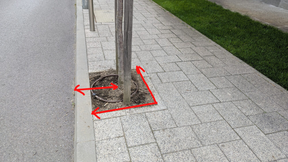
Пример за липса на отстояние и достатъчно открита почва – само 30 см. от бордюра и под 50 см. страна. Дървото никога няма да се развие и има нужда от напояване, за да е умре съвсем.
Тези изисквания не значат, например, че не може да се засади дърво точно до бордюра на пътя без достатъчно почва. Безсмислено би било, защото ще изсъхне, но също така не следва да се брои при смятането на озеленяването. Това е важно, защото освен дялът земя като зелена площ има изискване и какъв процент от нея е във висока дървесна растителност. За широколистни дървета с височина между 3 и 5 м. на 12 годишна възраст броят 12 кв.м. площ за това изчисление. Над 5 м. – 20. При иглолистните е съответно 5 и 7 кв.м.
Ключов аспект тук е, че доста от тези изисквания влизат в сила през юли 2023, т.е. за разрешения за строеж издадени преди това важат старите разпоредби за отстояния и почвен слой. През 2019 г., например, изискват да има почвен слой от поне 60 см., а когато е не по-малко от 30 см. площта важи с индекс 50% към общия коефициент на озеленяване. Отстоянията от бордюри, стени и тераси обаче са били същите.
Трябва да се разбере също, че плановете не са абсолютни. Това е просто илюстрация как си представят, че ще стане озеленяването, но на терен може да се окаже друго. Аналогично скиците къде ще бъдат сградите почти никога не отговарят в мащаб – отстоянията не са същите, височината не е тази и прочие. Затова ключовия момент е при приемане на обект на груб строеж да не се гледа по документи, а да се измерват реалната височина и отстояния. Аналогично при премателната комисия не се гледа дали точно в това пространство има дърво, а колко са на брой, дали са същия вид (има значение колко големи ще станат) и дали почвения слой и отстоянията са правилните.
Защо не виждаме тези планове?
Най-честата причина за отказ при поискване на тези скици, е че се засягали правата на трети лица. Това са инвеститорските компании и архитектите. Те от своя страна изрично са искали да не получавам плановете за озеленяване. Доколкото не изясняват никога в отговорите си точно какви права биха били засегнати и по какъв начин, може само да гадаем, че всъщност замесените се притесняват от разкриване на нарушения.
Подобни откази са доста спорни, защото става въпрос за документи неразделна част от строителните книжа. ЗУТ изрично посочва, че поне част от тях трябва да се публикуват в регистъра (когато види бял свят), т.е. са публични по дефиниция. Отделно свободно може да се използват в рамките на административен процес и производство, част от който спокойно да изиска публичността им какъвто вече в случая с исканията за промяна на ПУП и други аналогични скици от същите инвестиционни проекти. Няма основателна причина да се прилагат тези правила за публичност за едни чертежи, а не за други. Най-вече законът за достъп до обществена информация предвижда, че дори да има съмнение за засегнати права, при надделяващ обществен интерес може да се предостави достъп при минимизиране на предполагаемата щета. Т.е. могат да редактират имена и елементи, които ги притесняват и пак да предоставят скиците.
Експлоатиране на авторски права за прикриване
Попаднах и на друг аргумент – авторски права. Законът третира архитектурните планове и всичко свързано с градоустройството по любопитен начин. През последните 10 години са вкарани множество стратегически промени, които силно ограничават разпространението на архитектурни планове освен, ако изрично не се изисква от друг закон – например както ЗУТ дава възможност това да се определели с наредба. Тук ограничението сериозно надвишава опазване на имуществените и неимуществените права. Забранили са притежанието на копия от архитектурни планове дори за лична употреба без търговска цел.
Както се сещате, в тази хипотеза попадат и плановете за озеленяване като част от архитектурния проект. Те съдържат лични данни като кой ги е изготвил и подписал. Тези данни стандартно се заличават по GDPR. Това от своя страна създава интересна хипотеза – ако все пак получа тези скици със скрити имена и подписи, мога ли да спазя Закона за авторските права и да опиша както съм задължен източникът и авторът му, когато не го знам.
Голяма част от възможностите за т.е. „безкористно използване“ на авторски материали като журналистически материали, критика, сатира и прочие нарочно и изрично изключват тези свързани с архитектурата и градоустройството. Трудно ми е да определя тези точки като лобистки опити да се скрие ключова за обществото информация злоупотребявайки с принципите на авторското право. Аналогичен случай имах преди години, когато направих карта на разрешителните за сеч в България и няколко лесовъда ме заплашиха със съд, тъй като имали авторски права върху актовете и никой нямал право да ги използва без тяхно съгласие.
Административни документи в квантова суперпозиция
Всичко описаното до тук не важи за официалните актове и документи издадени от различните институции като част от административния процес. По принцип всички те са по подразбиране публични и специално тези по ЗУТ трябва вече да се публикуват от общини, ДНСК и министерства. Някои, които засягат вътрешни процедури и актове стават публични и обект на поискване по ЗДОИ две години след издаването им. Дори за тях никой държавен служител няма право да откаже предоставяне на вътрешните номера на такива документи, както и да признае съществуването им, освен ако не са засекретени. Тук няма значение дали същите се отнасят или засягат трети лица.
Това значи, че документ като протокола от държавната приемателна комисия, разрешението за ползване и всички документи издадени от общината и ДНСК следва да са публични и то най-късно две години след датата. Отделно копия от протоколите се дават на подписалите ги страни и членове на комисията.
Именно заради тези важни аспекти обжалвах два отказа на ДНСК да ми предоставят точно такива актове издадени от тях, както и протоколи по приемане. В тях се съдържа ключова информация какво са видели, какви забележки са имали и кой се е подписал, че всичко е наред. Делата са насрочени в рамките на следващия месец и се надявам до края на годината да имаме резултат.
Компромисният път
Авторските права в България са доста строги и подобни тенденциозни ограничения специално за архитектурата съвсем естествено притесняват всеки. Дори когато няма зла умисъл и опит за прикриване, това механично води до отказ от действие „за всеки случай“. Както споменах, ЗДОИ дава възможност да се търсят алтернативи при надделяващ обществен интерес. В случая несъмнено има такъв предвид изложеното в началото на този текст. Затова на няколко поредни искания за достъп до обществена информация от Столична община ми дадоха възможност да видя все пак плановете за озеленяване. Условието бе нямам дигитално копие, да ги чета само физически на място и да не правя снимки.
Това ми позволи да видя истинските параметри, разпределени на озеленяването, колко дървета, вертикално озеленяване и отстояния са обещали, както и как тези планове са се променяли с времето. Това е важно, защото често не знаем какво търсим докато не го видим. Не стига просто да се искат няколко числа от документите. Пробвал съм и дори такива са ми били отказвани с аргумента, че не им била работа да ровят по дигиталните архиви. Тази седмица получих такъв отказ по свързана тема, за която ще пиша също скоро. Нямах възможност да видя също протоколите от приемателната комисия, защото те са били при ДНСК, а районната администрация, където са разглежданите сгради и е била страна, отрича да има копие.
Затова в следващата част на тази статия няма да мога да ви покажа самите планове. Първо, защото години наред получавах откази от вече бивши главни архитекти. Второ заради ограниченията в закона за авторското право целящи именно избягване на подобна прозрачност. Трето, защото все още нямаме публичен регистър по ЗУТ, който да се надгради да включва документи защитаващи обществения интерес заедно с други подобни като транспортния анализ и становищата за пожарна безопасност.
Този начин на предоставяне е силно ограничаващ, най-малкото защото мога само да преразкажа какво съм видял на база няколко числа в наредбата. Ландшафт архитект би хванал с един погледа всички нередности, ако документите бяха публични. Все пак, Столична община направи една крачка повече от всички други институции и предишни администрации и ми даде поне някакъв достъп. Следващата стъпка би била довършването на регистъра по ЗУТ от Шишков и изискване да се качват този тип документи там.
В близките дни ще публикувам следващата част от темата, че която ще покажа с конкретни примери какво видях, какво липсва и защо е толкова нужна прозрачност и безкомпромисност.
To provide the best experiences, we use technologies like cookies to store and/or access device information. Consenting to these technologies will allow us to process data such as browsing behavior or unique IDs on this site. Not consenting or withdrawing consent, may adversely affect certain features and functions.
Functional
Always active
The technical storage or access is strictly necessary for the legitimate purpose of enabling the use of a specific service explicitly requested by the subscriber or user, or for the sole purpose of carrying out the transmission of a communication over an electronic communications network.
Preferences
The technical storage or access is necessary for the legitimate purpose of storing preferences that are not requested by the subscriber or user.
Statistics
The technical storage or access that is used exclusively for statistical purposes.The technical storage or access that is used exclusively for anonymous statistical purposes. Without a subpoena, voluntary compliance on the part of your Internet Service Provider, or additional records from a third party, information stored or retrieved for this purpose alone cannot usually be used to identify you.
Marketing
The technical storage or access is required to create user profiles to send advertising, or to track the user on a website or across several websites for similar marketing purposes.
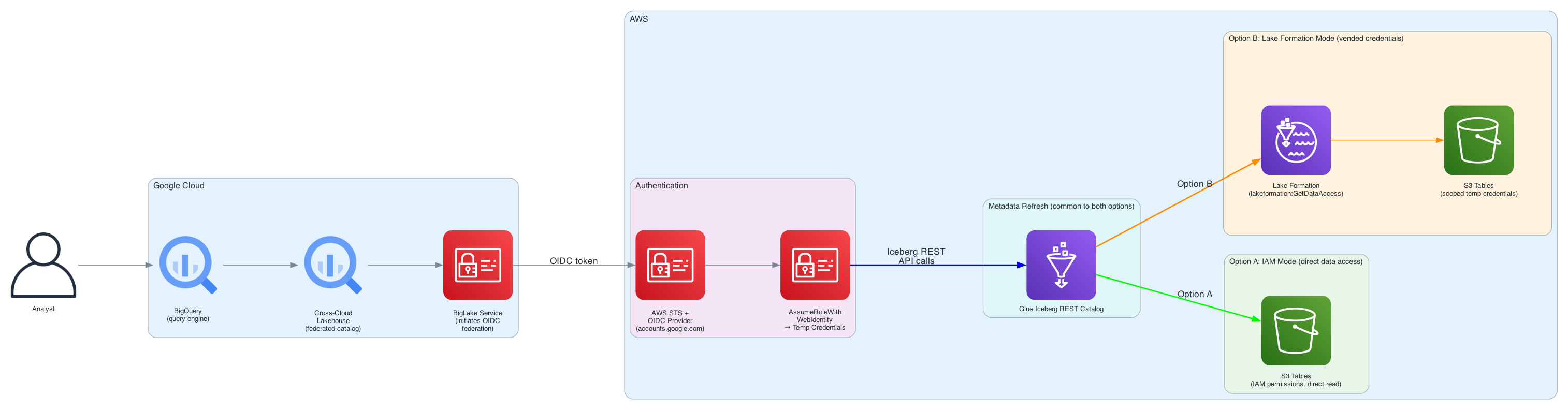

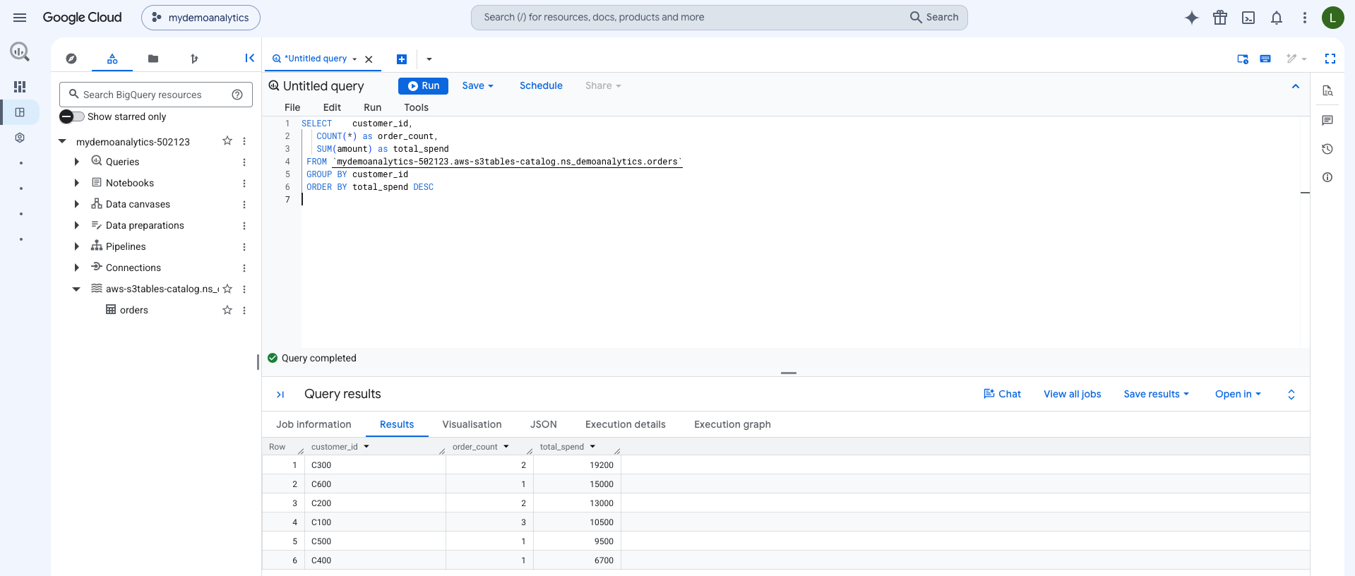
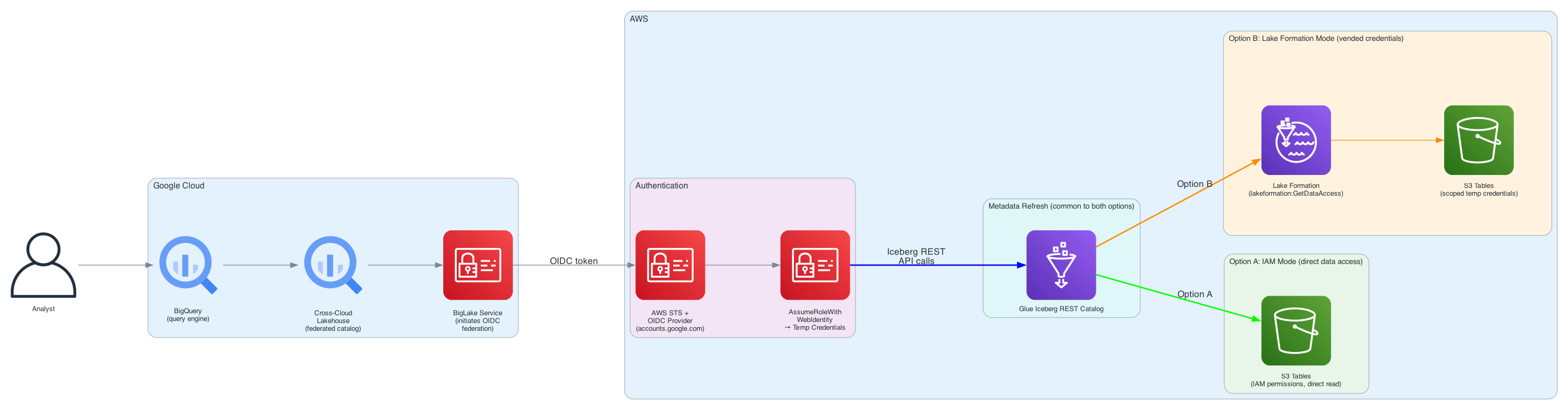
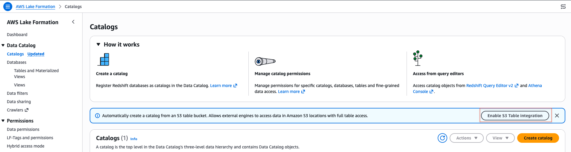
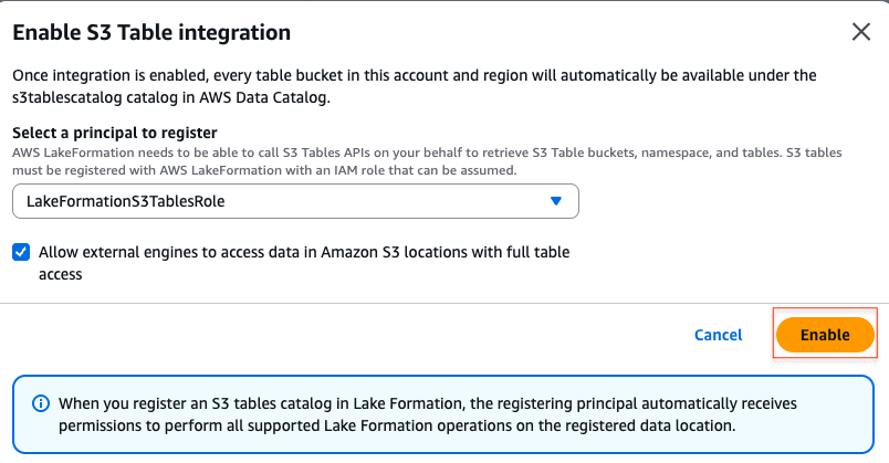
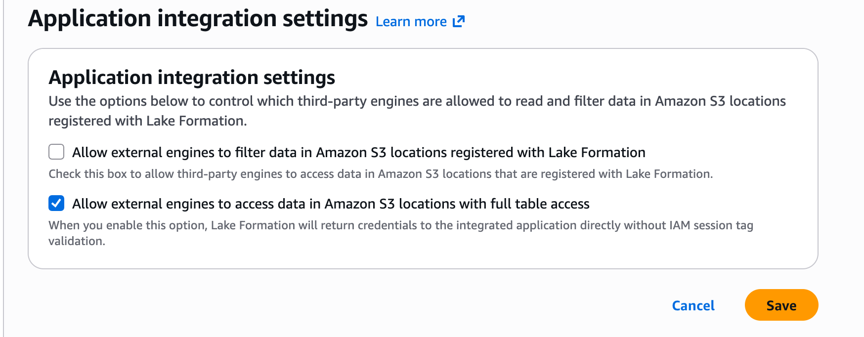
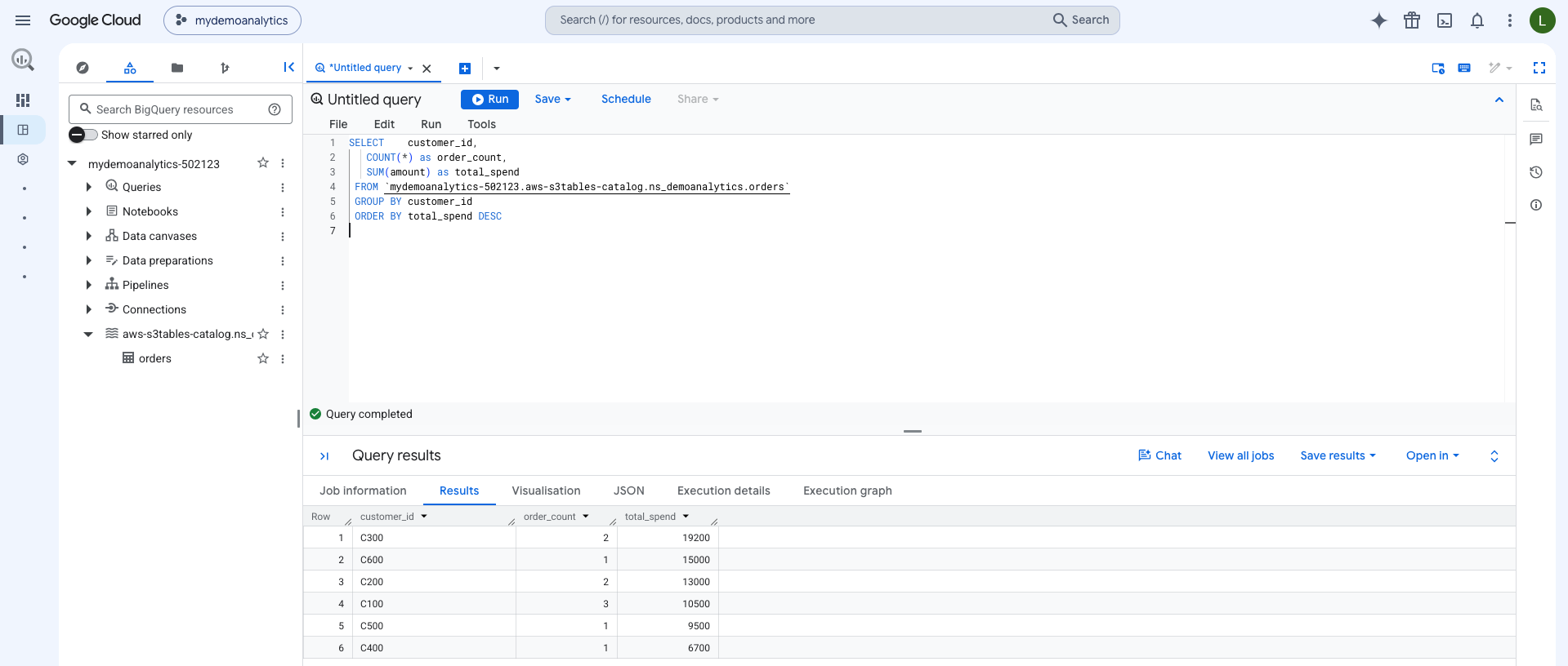
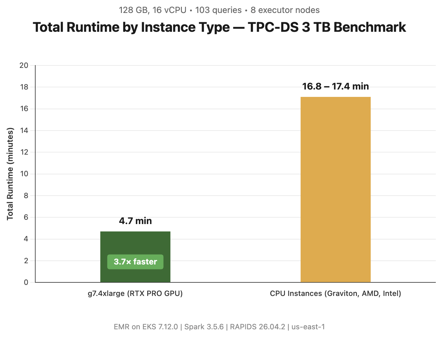
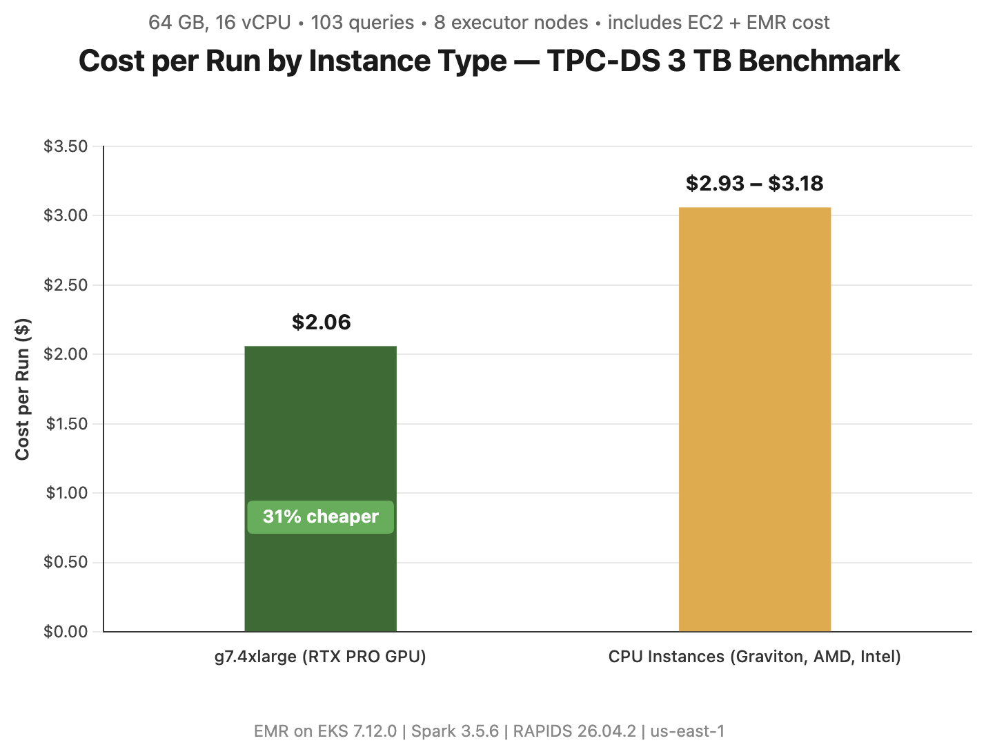
 Twenty years ago today,