Post Syndicated from corbet original https://lwn.net/Articles/1090099/
The
7.1.10,
6.18.46,
6.12.105,
6.6.153,
6.1.184,
5.15.217, and
5.10.266
stable kernels have all been released; each contains another set of
important fixes.
Post Syndicated from corbet original https://lwn.net/Articles/1090098/
From Jeremy Allison we have the
sad news of the passing of Steve French. He was the maintainer of the
kernel’s SMB filesystem code for many years, having only dropped that
role due to health issues in the last week. “I’ve known Steve for
” He will indeed be missed.
over 20 years. He was a legend in the community, and a really good
friend. He will be greatly missed. Farewell Steve.
Post Syndicated from Bozho original https://blog.bozho.net/blog/4622
„Троловете са на ДБ и ПП“. Тази лъжа тръгна от интервю вицепремиера по пропагандата Иво Христов и се поде от всякакви говорители, политици, журналисти.
Разбира се, ние в Демокртична България тролове нямаме.
Няколкото фейсбук страници, които бъркат в здравето на политическите манипулатори, не са наши и дори не познаваме хората, които стоят зад тях (с изключение на един от хората зад страницата BG Elves, когото познавам като местен активист).
Дали е редно политически мнения да се разпростаняват под псевдоним е отделен въпрос. Аз смятам, че е допустимо и част от културата в интернет. Но дори на страницата да пишеше „Зад страницата стои Иван Георгиев от Горна Оряховица“, нямаше да има особена разлика.
Но „трол“ значи друго и има друга цел – троловете са фалшиви профили, в общия случай без зад тях да стоят истински хора, чиято цел е да разпространяват и усилват дадено послание. Тролове могат да бъдат и обикновени хора, които със собственити си профили срещу заплащане да правят същото. А има и хибриден вариант, при който се плаща на обикновени хора да си направят по няколко акаунта – има такива репортажи по националните ни телевизии. Затова се говори за „ферми“ или „фабрики“ с тролове – защото бройката е много важна, за да бъдат подлъгани алгоритмите на социалните мрежи, че съдържанието, което харесват, споделят или създават е масово мнение.
Ние не само нямаме тролове, а сме единствената политическа сила, която е правила опити да намери решение на този проблем. И ще дам три примера.
През 2023 г. представихме публично законопроект, който целеше в определени случаи (допустими от гледна точка на хармонизираното европейско право) да задължим социалните мрежи да установяват координирано неавтентично поведение (т.е. профили, действащи по команда, най-често автоматизирано, да коментират/харесват/разпространяват дадено съдържание). Със законопроекта се предлагаха решения и на други канали за разпространение на пропаганда и дезинформация – напр. монетизирането на сайтове за фалшиви новини чрез фалшиви реклами – на хранителни добавки, фалшиви лекарства и др.
Тогава много от хората, които сега обясняват кой имал тролове, скочиха и казаха „сакън, цензура!“. Цензура, разбира се, нямаше, и от нас никога не би излязло нещо, което да отваря вратата за цензура, но тогава опитът за справяне с троловете беше удавен в такива заглавия и нравоучения.
През 2022 г., докато бях министър, на събитие в Давос, организирано от Украйна, говорих за ролята на социалните мрежи в борбата с разпространението на съдържание чрез координирано неавтентично поведение (тролове). Тогава имаше доклад на Фейсбук, че в месеците около нахлуването на Русия в Украйна, Фейсбук са свалили 2 фалшиви профила, свързани с Русия. Да, 2. Абсолютен провал – всички знаехме и виждахме какво се случва в социалните мрежи.
В този период имахме и срещи и кореспонденция с Мета на високо ниво. Изпратихме конкретно предложение – българското фейсбук пространство да бъде обект на задълбочено изследване за координирано неавтентично поведение. Мета отказа. В резултат на този отказ се роди и гореспоменатия законопроект.
Тогава от Мета ни попитаха „защо не използвате директния канал за докладване на съдържание“, на което моят отговор беше „защото не може правителството да казва кое е вярно и кое е грешно – ваша работа е да установите проблеми с поведението, а не със самото съдържание“.
Тази разлика е съществена. Винаги думата „цензура“ се появява, когато някой опита да говори по тази тема. А никога, по никакъв повод не е ставало дума за това държавата да определя кое е вярно и кое е „фалшива новина“ – това е гршено, опасно и не работи.
Пак тогава, през 2022 г. имах среща с двама еврокомисари в Брюксел – Тиери Бретон и Вера Йорова по отношение на същия проблем с троловете. Бретон поиска доклад с примери, какъвто подготвихме и му изпратих. Йоурова потвърди, че наблюдават същите проблеми с троловете и пропагандните наративи в Чехия, а и в много други източноевропейски държави. За съжаление Актът за цифровите услуги на ЕС беше в твърде напреднала фаза тогава и не беше възможно да се предложат допълнителни гаранции, че тролове няма да се използват за усилване на съдържание.
Все пак, Актът за цифровите услуги даде инструментариум на Европейската комисия да изисква мерки срещу това поведение. И това дава някакъв резултат. В последната предизборна кампания ТикТок свали 34 фалшиви профила на ДПС.
А Иво Христов вероятно може да разкаже повече за това кои профили, промотиращи Прогресивна България са били свалени от ТикТок и защо. Вероятно затова тогава Радев подскочи и заговори за „румънски сценарий“ ни в клин, ни в ръкав. Може би има обяснение и за десетките профили, пускащи едно също съдържание в подкрепа на ПБ, които бяха осветени в последните дни.
Пиша всичко това, за да не бъде подменяна реалността – нещо, което вероятно е добре описано в кремълските учебници по пропаганда. Учебници, които са успешно адаптирани за дигиталната ера.
Но както писах и онзи ден по друг повод – би било грешка да обвиним руската пропаганда за всички несгоди – най-малкото защото има достатъчно местни играчи, които си мислят, че като платят на „агенция“, която да организира тролски профили да им слагат сърчица, ще подквасят политическото море.
Различното мнение не значи, че някой е трол. Установяването на тролове е много лесно за Фейсбук и много трудно за странични наблюдатели, които не разполагат с метаданни. Трудно е, но не невъзможно да бъде намерено решение на този проблем и призовавам да търсим такова, вместо вицепремиери да си споделят фрустрациите от 3-4 анонини страници.
Материалът Чии са фейсбук троловете? е публикуван за пръв път на БЛОГодаря.
Post Syndicated from Oglaf! -- Comics. Often dirty. original https://www.oglaf.com/calculus/


Post Syndicated from LastWeekTonight original https://www.youtube.com/watch?v=juCyYV7kauw
Post Syndicated from Patrick Kennedy original https://www.servethehome.com/patrick-at-micro-center-columbus-ohio-grand-reopening-with-jeff-geerling/
Patrick and Jeff Geerling are at the Micro Center in Columbus, Ohio for the new store’s grand reopening today
The post Patrick at Micro Center Columbus Ohio Grand Reopening with Jeff Geerling appeared first on ServeTheHome.
Post Syndicated from The Atlantic original https://www.youtube.com/shorts/DF7Ns4tr2q0
Post Syndicated from Techmoan original https://www.youtube.com/watch?v=x0og-gbDPTs
Post Syndicated from Jin-Hee Lee original https://blog.cloudflare.com/bot-preference-sync%20/
We’re constantly building for the different goals of our customers. Some customers want to optimize for discovery, while others want to protect their content with the strictest security policy. Among these differing policies, there are multiple ways to mitigate bot traffic. Some mechanisms simply state your preference, assuming best intent from crawlers, and other approaches actually lock down content by outright blocking with a Bot Management solution.
We recognize that it's cumbersome to maintain multiple layers of protection on your website. For example, there are cases in which your robots.txt states that a crawler is Disallowed from accessing your website, while your enforcement rules actually don’t block that crawler. When your stated preferences and your enforced rules disagree, some crawlers treat it as a basis to disregard your preferences or try to bypass your enforced rules.
A couple of years ago, Cloudflare announced an easier way to disallow AI training on your website by tackling two of these layers: a managed value of robots.txt that told a fixed list of major Training crawlers not to train on your content, along with edge-enforced blocks to Training crawlers. On July 1, 2026, we launched easier options to manage different kinds of AI traffic use cases. You can say what you want to do about Search, Agent, and Training traffic on your website.
We're announcing Bot Preference Sync, available to all customers from the Free tier to Enterprise. Bot Preference Sync reflects what you've set in your AI bot configuration by updating corresponding preferences to your robots.txt, and it can be turned on or off at any time. No more static file for one use case: we'll help you tailor your robots.txt to reflect what you’ve already configured for different AI bot categories.
For years, the most pressing question in this space was: "Is my content being used to train AI models without my permission?" It's an important question, and it isn't going away. Alongside this, the questions we increasingly hear are about discoverability and engagement. How do I show up when someone asks an AI assistant something my site can answer? How much of my traffic is coming from AI crawlers versus real people? What content is actually driving referrals, and what is it worth?
The answers differ by business model. Discoverability and engagement are key, top-of-mind issues for any businesses trying to thrive on the modern web, but the funnels for these are different: an e-commerce store may want everything crawled and trained on, so its products surface when a shopper asks a chatbot for "the best sofa for a small apartment." A publisher that monetizes pages with ads may want the opposite: stay in the search index that sends readers to the page, but keep its articles out of model training and, crucially, be able to verify that its content really wasn't used without permission.
There's no single right answer, which is exactly the point. Your controls should reflect your strategy, which is why we've been building tools to give you visibility and choice at every layer. Bot Preference Sync ties these together, so the preference you set is the preference you publish.
On July 1, 2026, we made the case that mixed-use crawlers, or “bots that blend search, agent use, and training behind a single user agent,” put site owners at a disadvantage precisely because they make it hard to separate what you want from what you don't. That's still true, and our position on Transparency for site owners hasn't changed.
But there’s more than one way to approach Transparency. We want to reward the operators who are clear about their identity and how they are using the data they crawl. For purposes of bot Verification, the owners of bots that perform both Search and Training will need to provide additional information in order to not be blocked when “Disallow Training” is set. Those requirements are:
Bots of leading AI models and service providers that meet these criteria are tracked publicly in the AI bot transparency section in Cloudflare Radar, which includes examples in which best practices are honored, as well as when they are not. Crawlers that don't provide Transparency will not get the benefit of the doubt — they're still blocked when you disallow training. In other words, this is a way of making Transparency the price of admission.
Bot Preference Sync is a new feature that keeps your robots.txt reflecting the AI bot preferences you've already set for Search, Agent, and Training on the Cloudflare zone-level dashboard. If a site owner already has a robots.txt file, the contents added by Bot Preference Sync will be prepended to the existing material, so any existing Disallow directives are maintained.
Instead of a site owner maintaining a separate static file, Cloudflare generates or updates your robots.txt based on your configuration, so what you say to the world and what you enforce at the edge are kept in sync.
For Search and Agent, the three options we announced on July 1 remain: Allow, Block on pages that serve ads, or Block everywhere. For Training, we’re refining the option to stop your content being used for training models with the Disallow option:
Disallow: a "no training" preference is written to your robots.txt, so that cooperating mixed-use crawlers who take the extra Transparency step can still access your content for search indexing, since they’re allowing site owners to directly verify how their data is used. Cooperating crawlers honor the preferences in robots.txt, and your Search visibility for cooperating crawlers is unaffected.
Let’s take the example below, in which someone has configured their AI bot policy to say “Allow Search, Allow Agents, Disallow Training.”
Since this example site has Bot Preference Sync on, their robots.txt would prepend something like the following (which has been shortened and anonymized for the sake of the example):
We’ll use bots that we track in BotBase to periodically update the list of bots that is added to robots.txt when you choose to Block or Disallow a given category. The Verified bots that are classified as Search, Agent, and Training can be viewed at any time in our public bots directory.
For all new customers, Bot Preference Sync will be on by default, to make it easier to manage blocks and preferences that reflect the same policy. For existing customers who are using the legacy managed robots.txt feature, we'll prompt you to review and confirm your preferences to transition to the new Bot Preference Sync upon its upcoming launch.
Some customers may want or need to be more hands-on in stating their preferences, for example, if they have a special arrangement with a given company to which they want to grant an exception. Because Bot Preference Sync is designed to tackle policy decisions made category-wide rather than case-by-case, it will not directly read from individual custom rules with more complex logic. Customers with a more fine-tuned security policy always have the option to turn off the sync that sets group policies, and tailor their file to match their custom policy.
We’re also making a change that allows publishers or ad-supported sites to have a different default from other site owners. We’ve created a default to make it easier for publishing sites that rely on ads and expect them to be reserved for human visitors. At the time of onboarding, such customers can select the option, “I monetize from pages with ads on this domain", which will set Training to Disallow as the default. (Customers have the choice to change this setting at any time.) This way, you stay in search while keeping your content out of model training.
For the non-publisher case, new customers will not have any blocks or disallows added by default when they onboard a domain: the choice is up to the customer. You can choose if you want to block Search or Agent or Training at any point, but the starting point will not add any blocks on your behalf.
Bot Preference Sync will be available to all customers, on every plan, in the coming week. Keep an eye on our changelog for availability, and watch your dashboard (and inbox) for the prompt to confirm your preferences!
This is one step in a longer effort. We'll keep working with the large bot operators to make sure we're not compromising on familiar challenges (like training without consent) nor emerging questions (like discoverability and engagement). Beneath it all is our effort to promote greater Transparency and control for site owners.
Post Syndicated from Bruce Schneier original https://www.schneier.com/blog/archives/2026/08/friday-squid-blogging-neon-flying-squid.html
The neon flying squid can fly in formation.
The shoal of about 100 squid rose unexpectedly from a patch of the Pacific Ocean around 370 miles from Tokyo and glided near the boat for about 30 metres. The astonished researchers were the first to capture photographs of such a thing, which looked like the early stages of an alien invasion.
They were probably neon flying squid (Ommastrephes bartramii), the subsequent study states, a species that is part of a 20-strong flying squid family that was known to leap from the water but, until then, was only rumoured to also be able to glide above it.
The neon flying squid was able to gain such elevation by using the hyponome, a funnel-like muscular organ also present in other cephalopods, such as octopuses. The organ is able to force water out in a jet, propelling the body along both in and out of the sea. Photographs of the gliding squid show them with their arms (they have 10 limbs in all) splayed outwards.
As usual, you can also use this squid post to talk about the security stories in the news that I haven’t covered.
Post Syndicated from Channy Yun (윤석찬) original https://aws.amazon.com/blogs/aws/aws-glue-6-0-now-available-with-30-lower-price-and-full-apache-iceberg-v3-support/
Today, we are announcing the general availability of AWS Glue 6.0, delivering 30% lower pricing than previous AWS Glue versions and introducing full support for Apache Iceberg v3 features. AWS Glue 6.0 is built on a fully modernized runtime, Apache Spark 4.1, Python 3.12, and Scala 2.13, delivering faster performance.
With this release, AWS Glue provides the most complete Iceberg v3 implementation on any fully serverless managed Spark service, along with new capabilities that simplify ETL authoring, improve PySpark performance, and enable real-time streaming with single-digit millisecond latency.
What is new in AWS Glue 6.0
AWS Glue 6.0 delivers the complete Apache Iceberg v3 specification, built on Iceberg 1.11.0. The headline feature is the VARIANT data type with shredding support, which achieves faster query read performance compared to traditional string data type columns for semi-structured data.
With VARIANT shredding, you can store and query JSON, logs, and event data without flattening schemas, eliminating duplicate data copies, custom parsing code, and pipeline breakage when schemas change. This capability transforms how teams handle semi-structured data at scale.
Additional Iceberg v3 capabilities include:
AWS Glue 6.0 also includes most significant upgrade in Spark 4.1, the modern runtime engine:
Getting started with AWS Glue 6.0
No API changes are required to use AWS Glue 6.0. You can select the new version using the existing --glue-version parameter in the create-job or update-job APIs through AWS Command Line Interface (AWS CLI), AWS SDK, AWS Glue Studio, Amazon SageMaker Unified Studio, and your preferred IDE.
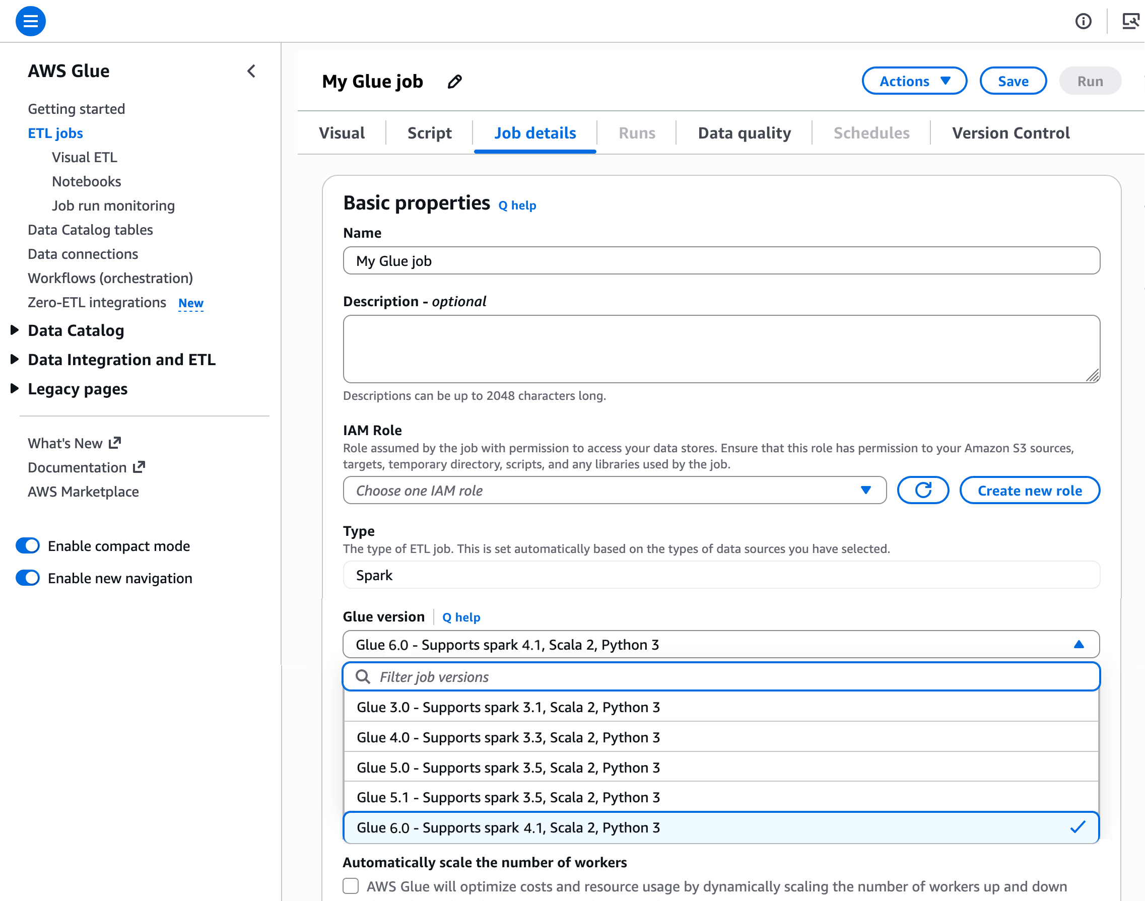
To get started with AWS Glue 6.0 jobs in the AWS Glue Studio console, open the AWS Glue job and on the Job Details tab, choose the version Glue 6.0 – Supports Spark 4.1, Scala 2, Python 3. You can create new AWS Glue jobs on AWS Glue 6.0 to get the benefit from the improvements, or migrate your existing AWS Glue jobs.
To start using AWS Glue 6.0 on an AWS Glue Studio notebook or an interactive session through a Jupyter notebook, set 6.0 in the %glue_version magic. You can also upgrade existing jobs to Glue 6.0 using the Spark upgrade agent on AWS Glue Studio or use the auto-upgrade feature in their existing Glue jobs to automatically upgrade them to Glue 6.0.
To learn more, visit the AWS Glue 6.0 version detail and Migrating AWS Glue for Spark jobs to AWS Glue version 6.0 in the AWS documentation.
Now available
AWS Glue 6.0 is generally available today in all AWS Regions where AWS Glue operates. For Regional availability and a future roadmap, visit the AWS Capabilities by Region. If you want to call APIs, search documentation, find regional availability, and check troubleshooting about this new feature, try using the AWS MCP Server and plugins with your preferred AI tool.
You pay an hourly rate, billed by the second, for crawlers (discovering data) and extract, transform, and load (ETL) jobs (processing and loading data). For the AWS Glue Data Catalog, you pay a simplified monthly fee for storing and accessing the metadata. The first million objects stored are free, and the first million accesses are free. To learn more, visit AWS Glue Pricing page.
Give it a try in the AWS Glue Studio console, and send feedback to AWS re:Post for AWS Glue or through your usual AWS support contacts.
— Channy
Post Syndicated from Dhananjay Karanjkar original https://aws.amazon.com/blogs/architecture/build-a-unified-ai-agent-architecture-with-dynamodb-and-bedrock/
Teams building AI agents on AWS often face a fragmented data architecture: operational data lives in Amazon DynamoDB while vector embeddings for semantic search sit in a separate, purpose-built vector store. This duplication increases infrastructure cost, adds synchronization complexity, and widens the window for stale retrieval results. With the general availability of native vector search in Amazon DynamoDB (launched August 5, 2026), you can now store embeddings alongside your operational data in the same table. You query them using the SearchVectors API operation.
In this post, I show you how to build a unified AI agent architecture where an Amazon Bedrock agent uses a single DynamoDB table for both structured lookups and semantic similarity search. The agent calls AWS Lambda action groups that invoke SearchVectors for natural language retrieval and standard DynamoDB APIs for create, read, update, and delete (CRUD) operations. An Amazon DynamoDB Streams pipeline automatically generates embeddings using Amazon Titan Text Embeddings V2 whenever content changes. This keeps the vector index synchronized without manual intervention.
Consider a technical knowledge management platform where a team maintains hundreds of internal documents: runbooks, architecture decision records, and troubleshooting guides. Team members interact with a conversational agent to find relevant content (“What’s our retry strategy for payment failures?”), retrieve specific documents by ID, or update existing entries.
Without native vector search, this architecture requires a DynamoDB table for document storage plus a separate vector database (or Amazon OpenSearch Service cluster) for semantic retrieval. The Amazon DynamoDB Streams pipeline must write to both stores, and the agent must route requests to the correct backend. With DynamoDB vector search, you collapse this into a single table and reduce operational overhead.
This solution uses a single-table design in DynamoDB that serves two access patterns: key-value lookups for operational data and approximate nearest neighbor (ANN) search for semantic queries. A Bedrock agent orchestrates user interactions and routes requests to the appropriate action group function.
The following list summarizes the core components:
SearchVectors) and CRUD operations against the same table.The following diagram illustrates the data flow through the unified architecture.
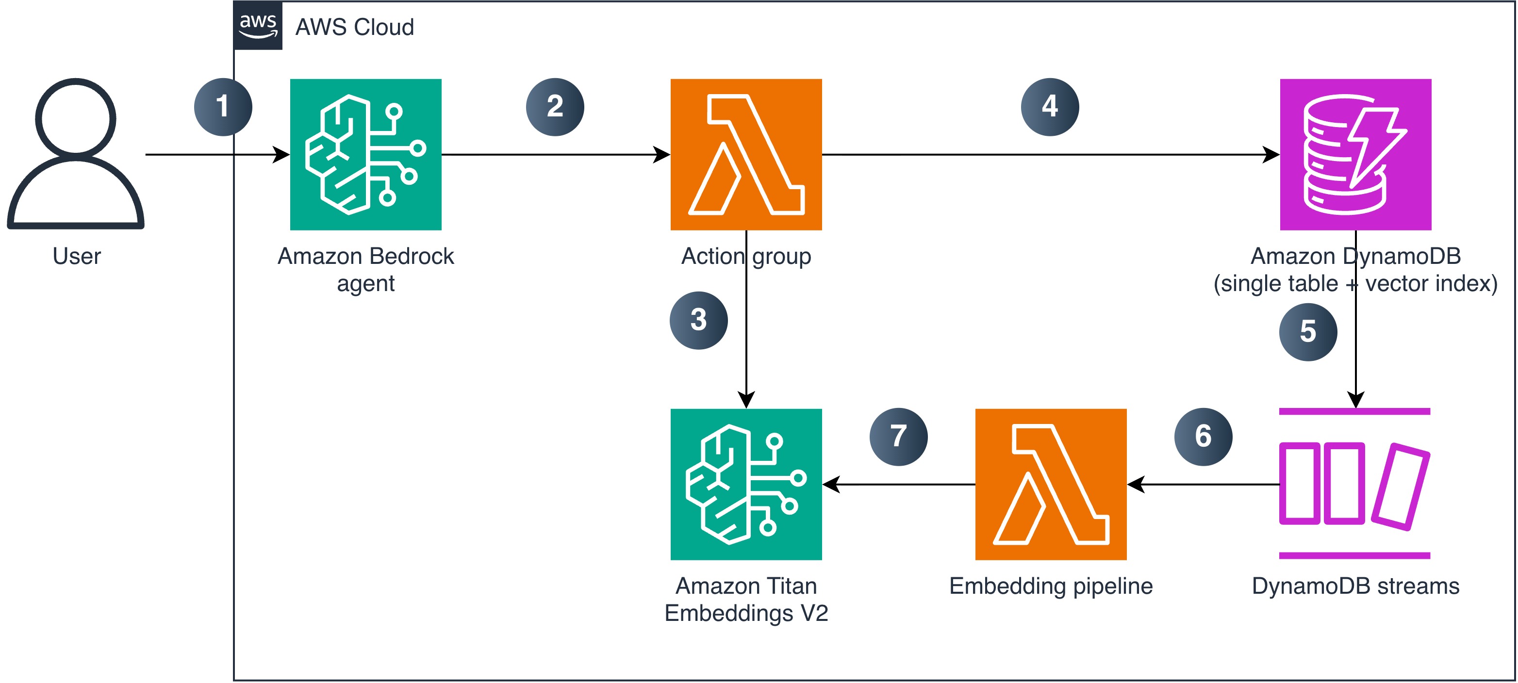
Figure 1: Unified AI agent architecture using DynamoDB vector search and Amazon Bedrock
The numbered steps describe the data and request flow:
SearchVectors API (or standard CRUD APIs for operational lookups) against the single table with vector index.To implement this architecture in your account, you need the following:
StreamViewType set to NEW_AND_OLD_IMAGES (the embedding pipeline compares old and new content to prevent a write loop).amazon.titan-embed-text-v2:0) enabled in Amazon Bedrock model access.This section walks through the key components of the architecture.
The table uses a composite primary key (entity_id as partition key, sk as sort key) and stores embeddings as a list of numbers:
The vector index partitions search results by the category attribute. Choose a partition key with moderate cardinality that matches your query patterns. A very low-cardinality key (a handful of values) concentrates data in few partitions and limits throughput scaling, while a unique-per-item key leaves no neighbors to compare. For multi-tenant workloads, tenant_id is usually the right partition key. For more information, refer to the DynamoDB vector search best practices.
The following AWS Command Line Interface (AWS CLI) command creates the vector index on an existing table:
After creating the index, wait for it to become searchable. Poll DescribeTable until IndexStatus is ACTIVE and Backfilling is no longer true. The first few searches after the index reports ACTIVE can still return ValidationException because SearchVectors is served by a dedicated search endpoint. Treat these as retryable rather than as a failure.
Key constraints to keep in mind:
SearchSchema HASH attribute is mandatory in every SearchConditionExpression.SearchVectors responses are limited to 16 MB and don’t support pagination. Project only the attributes you need and keep TopK modest to stay within this limit.SearchSchema HASH attribute (category in this example) are silently excluded from the vector index while remaining in the base table.The action group Lambda handles both semantic search and operational lookups. The agent invokes it with a function name and parameters based on the tool definition.
The semantic search function generates a query embedding and calls SearchVectors. This index uses COSINE distance, where lower scores indicate greater similarity. Name the field accordingly so the agent doesn’t invert the ranking:
The generate_embedding helper calls Amazon Titan Text Embeddings V2:
The Lambda handler routes requests based on the function name passed by the Bedrock agent:
The embedding pipeline Lambda triggers on INSERT and MODIFY events. It generates an embedding for new or changed content and writes it back to the same item:
The infinite-loop guard is critical. Without it, the Lambda writes back an embedding, which triggers another Streams event, which triggers another embedding generation, and so on. The check compares the content field between old and new images, skipping processing when only the embedding attribute changed. This guard requires StreamViewType = NEW_AND_OLD_IMAGES. Without it, OldImage is empty and the guard never fires.
For production use, configure the event source mapping with ReportBatchItemFailures so that only failed records are retried. Add an Amazon Simple Queue Service (Amazon SQS) dead-letter queue (or on-failure destination) for records that repeatedly fail. Retry Amazon Bedrock InvokeModel calls with exponential backoff to handle throttling.
The Bedrock agent needs a function schema that describes the available tools. This tells the agent when and how to call each function:
This unified architecture works best when your application already uses DynamoDB as its primary operational store and you want to add semantic search without managing a separate service. Consider the following decision points:
TopK limit.The following list highlights the key security aspects of this architecture:
dynamodb:SearchVectors to the specific index ARN (arn:aws:dynamodb:{region}:{account}:table/{table}/index/{index}). The embedding Lambda needs only dynamodb:UpdateItem, not search permissions.dynamodb:LeadingKeys don’t apply to the SearchVectors API. For multi-tenant workloads, use the SearchSchema HASH partition key to scope queries by tenant, or use separate tables for strict isolation.SearchVectors traffic uses TLS. The API routes to a dedicated search endpoint that the AWS SDKs handle automatically.bedrock:InvokeModel permissions to the specific embedding and agent foundation model ARNs required by the solution.lambda:InvokeFunction to bedrock.amazonaws.com on the action group Lambda, scoped with an aws:SourceArn condition matching the agent ARN. Without this resource-based policy, the agent can’t invoke the action group.To avoid ongoing charges, delete the resources in the following order:
With this pattern, you can build a unified AI agent architecture that uses a single DynamoDB table for both operational data and vector-based semantic search. The native vector search of DynamoDB combined with Bedrock agent action groups eliminates the need for a separate vector database. DynamoDB Streams-driven embedding generation keeps the index synchronized in real time.
This pattern reduces infrastructure complexity for applications that already rely on DynamoDB and need to add conversational AI capabilities. The automatic embedding pipeline keeps your vector index synchronized with operational writes, and the action group design gives the agent access to both semantic and structured query paths.
Adapt the table schema, embedding dimensions, and agent instructions to your domain. Clone the sample-dynamodb-vector-search-architecture repository to deploy the complete working implementation. For more information about DynamoDB vector search capabilities and limits, refer to the Amazon DynamoDB vector search documentation.
Post Syndicated from Technology Connextras original https://www.youtube.com/watch?v=fHPCS8j3cRM
Post Syndicated from Bruce Schneier original https://www.schneier.com/blog/archives/2026/08/ai-is-learning-to-write-genetic-code.html
This sort of research is both exciting and terrifying:
The two models in question were told to generate complete genomes for a viable bacteriophage—a type of virus able to infect and replicate itself inside bacteria, destroying them from the inside.
Using an existing bacteriophage as an example—ΦX174 (pronounced “fie-ex-1-7-4”), known for its ability to infect and destroy E. coli bacteria—the models generated about 700,000 potential designs, of which the researchers picked 285 that looked most promising.
The researchers then synthesised new DNA molecules using those designs and inserted them into E. coli bacteria, before waiting to see if viable bacteriophages would emerge.
Shortly afterwards, 16 of the Petri dishes in which the bacteria were growing began to show clear spots, as the viruses began to attack and replicate themselves inside the E. coli, demonstrating their viability.
Some of those viable viruses proved more effective at attacking E. coli than the original ΦX174 bacteriophage.
That’s a positive use of a synthetic virus. We can all imagine the negative uses.
Post Syndicated from Patrick Kennedy original https://www.servethehome.com/bosgame-m5-amd-ryzen-ai-max-395-128gb-ai-desktop-review/
We tested the Bosgame M5, an AMD Ryzen AI Max+ 395 system that is one of the lowest cost 128GB LPDDR5X local AI systems out there
The post Bosgame M5 AMD Ryzen AI Max+ 395 128GB AI Desktop Review appeared first on ServeTheHome.
Post Syndicated from Netflix Technology Blog original https://netflixtechblog.com/a-tale-of-two-flink-autoscalers-e9f6a1b1492b
Samuel Yeboah, Francesco Di Chiara and Mingliang Liu
Today, Netflix runs two Flink autoscalers. That is exactly one more than we want. We built the first one in-house years ago, when there was no mature option suited to our platform. The second came from the Apache Flink community, and it can scale workloads our homegrown system was never designed for. We now run both in production and are steadily converging on the open-source one. Along the way we learned some hard lessons about metrics, cost, and the real price of maintaining infrastructure you could instead adopt, and we hope they are useful whether you run a handful of Flink jobs or tens of thousands.
Netflix has run stream processing on Apache Flink since 2017. As of 2026 we operate more than 30,000 Flink jobs across multiple AWS regions. Most are not deployed by hand; they are generated by our managed platform Data Mesh, so the majority of users never touch a Flink job directly. A smaller but growing set are custom jobs, built and operated by teams across the company for use cases like personalization, Ads, and Live events. They range from single-operator jobs that shuttle records between Kafka topics to stateful pipelines with branches, joins, and terabytes of state, and their load swings with daily cycles, launches, and regional failovers.
Provisioning every one of those jobs for its peak is wasteful; provisioning for the average causes lag during surges. And in our platform a scaling action is not free: by default it means taking a savepoint, stopping the job gracefully, and restarting it at the new size, which for a large stateful job can take minutes. That leaves a genuinely hard question: how do you give each job the resources it needs, when it needs them, without a human in the loop and without breaking anything?
Our first answer, built around 2019, was an autoscaler shaped like a stream-processing job. It ran on Mantis, consuming a live feed of cluster-level metrics from Atlas, our telemetry platform including CPU, network, Kafka lag, input-rate, and consume-rate signals for every job. The scaler combined lag-derived catch-up time, CPU/network utilization thresholds, observed performance history, and regression over recent input rate to decide when to scale up or whether a smaller cluster could handle the lookahead window. Because the autoscaler operates independently of the Flink platform, it remains unaffected by issues within Flink itself. Building it as a streaming job also made it easy to scale. Each autoscaler node handled the metrics for a subset of Flink jobs, and we never had to write custom sharding or coordination logic to keep up with a growing Flink fleet. It reliably cut resource usage by 25–45% across thousands of managed pipelines. Check our previous talk at Flink Forward 2020.
But watching from outside has a ceiling. The system reasoned about a whole cluster through coarse container metrics, and it scaled a single knob, the total TaskManager count, so every operator in a job moved together. That fit the simple, single-operator pipelines it was built for, but not the multi-operator, stateful DAGs that teams were increasingly bringing to us for Ads, recommendations, and games. Those were exactly the jobs it could not reason about, and supporting each new case meant more custom logic rather than any general capability.
The autoscaler is only as good as the metrics served by external systems beneath it. Those metrics could miss real trouble: a job could be completely busy without any of it showing up as CPU utilization, leaving the job stuck in a degraded state the scaler had no way to see. Recently a networking migration quietly changed how some traffic was reported, and a subset of the Atlas metrics the scaler relied on stopped capturing everything accurately. The gap stayed invisible until it surfaced in production much later.
It was time to reconsider build versus buy.
When we started, the Flink community had no mature autoscaler to offer. By the time we re-evaluated, it did: the Apache Flink Autoscaler. Instead of watching containers from outside, it reasons from inside the job.
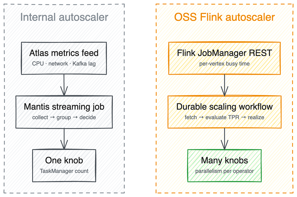
Its key idea is to estimate each operator’s true processing rate (TPR): the throughput it could sustain if it were fully busy. Flink reports, per subtask, the fraction of each second spent doing actual work, separate from time spent backpressured or idle. Dividing observed throughput by that busy fraction extrapolates capacity to full utilization: an operator handling 700 records/sec while busy 70% of the time has a TPR of 700 / 0.7 = 1,000 records/sec. Starting from the sources, the autoscaler walks the job graph and uses each operator’s TPR, its input/output ratios, and a target utilization to compute the parallelism every vertex needs so that no operator becomes the bottleneck, rather than resizing the whole cluster as a unit.

The two approaches make a different contract, summarized below.
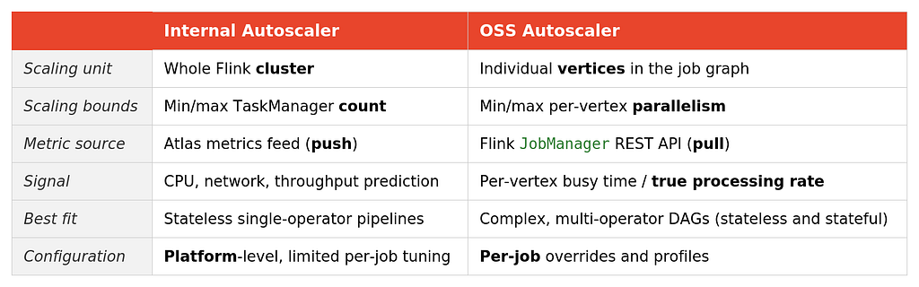
The decisive difference for us is the last two rows: the OSS autoscaler can scale exactly the stateful, multi-operator jobs our homegrown system could not, and it lets each job carry its own configuration — stabilization periods, thresholds, and other scaling behavior tuned to the workload.. That made it the natural fit for the custom jobs teams had been scaling by hand.
Adopting the algorithm was straightforward; the community had done the hard part. The work for us was running it reliably across our own jobs, and this is where our system differs most from the stock open-source deployment.
Firstly, the OSS autoscaler was originally architected to reside within the Kubernetes Operator for Flink, but our Flink platform runs on its own control plane, not that operator (see our previous talk at Current Conference 2024). Community later made a fantastic decision to keep the core logic as a standalone library. They refactored four generic interfaces that made it easy to plug directly into our internal ecosystem: a context carrying job metadata and REST API info, a state store, an event handler, and a realizer that applies scaling decisions.
That service is a Spring Boot application whose orchestration runs on Temporal, the durable workflow engine. An orchestrator workflow polls our Flink control plane about once a minute for the jobs with autoscaling enabled, and starts one long-running workflow per job. Each per-job workflow pulls that job’s per-vertex metrics from its Flink JobManager, runs the OSS evaluation algorithm, and, when a scaling decision results, hands it to a realizer that actuates the change through our Flink control plane.
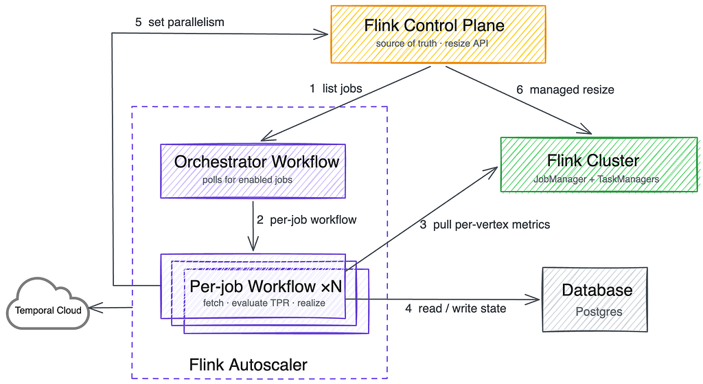
The workflow-per-job design was a direct response to pain. We first ran evaluations in a single batch loop over the whole set of jobs, and it was fragile: one slow or misbehaving job could stall metric collection and scaling for every job behind it. Giving each job its own durable workflow isolated that blast radius, so a single problematic job now fails and retries on its own, and the runtime scales out as we onboard more jobs.
Secondly, three engineering gaps stood between “works in community” and “works at Netflix scale”:
Before it actuates anything, the realizer runs a set of safety checks. For example, it refuses to scale a job down in a region being evacuated during a company-wide region failover. It also verifies there is enough disk for the new cluster to hold the job’s checkpoint state, and it adds a small standby buffer for larger clusters.
Last year, the OSS-based autoscaler achieved general availability for custom jobs at Netflix, yielding promising initial outcomes. For instance, our client telemetry and logging team achieved a 58% reduction in its annualized Flink compute expenditures, saving approximately $1.1 million annually. This efficiency is driven by three key factors. First, whereas static provisioning must always account for peak loads, autoscaling dynamically adapts to daily cycles, capturing the drop in traffic during nights and weekends compared to weekday peaks. Second, rather than relying on teams to manually optimize resources following performance improvements or post-holiday slowdowns, the autoscaler continually adjusts capacity. Finally, adopting uniform container dimensions enables superior bin-packing and more granular scaling increments.
Additionally, scaling down too eagerly is its own trap. Cut too deep and CPU saturates, lag spikes, and the system cannot react instantly because its metric window and stabilization period have to rebuild after each restart. We now run a target utilization of 0.45, below the community default of 0.7, deliberately trading a little efficiency for stability. Fewer and calmer rescales are worth the marginal cost for large stateful jobs.
While our scaler provides fine-grained signals and vertex-level decision units for stateful DAGs, fast rescaling still heavily depends on Flink Core’s state restoration performance. Today, the biggest remaining cost in scaling a stateful job isn’t the scaler’s logic — it’s the restart and state recovery process itself. Flink 2 addresses this through its disaggregated state architecture, keeping state in external storage rather than on local disk, which can sharply reduce how much a rescale or recovery depends on total state size. Having started supporting Flink 2.2 at Netflix, we plan on experimenting with this new state backend to see if it can help eliminate state recovery bottlenecks when scaling large stateful jobs.
Looking ahead, we aim to migrate all internal scaler use cases onto the new one based on OSS autoscaler to simplify our operational surface area.
Along the way, three lessons that generalize beyond Flink:
Thanks to the Flink and Data Mesh teams for the control-plane changes this work depended on, to the Temporal team and our early pilot teams, and to the Apache Flink autoscaler maintainers whose foundation we built on. Special thanks to Andy Zhang, Calvin Cheung, Daniel Trager, Guil Pires, Mark Cho, Matthew Kornitsky, Nikhil Sulegaon, Sujay Jain, and Tom Lee.

A Tale of Two Flink Autoscalers was originally published in Netflix TechBlog on Medium, where people are continuing the conversation by highlighting and responding to this story.
Post Syndicated from LastWeekTonight original https://www.youtube.com/watch?v=wB9bkcHwq4w
Post Syndicated from Боян Юруков original https://yurukov.net/blog/2026/bulgariaads/
Всички забелязваме колко много реклама – най-вече такава на хазарт – има по улиците и пътищата на страната, по билбордове, фасади, покриви и какво ли не. Наскоро реших да науча повече как се получава така. Разгледах първо положението в София и създадох инструмент, с който всеки може да провери какви разрешения за реклама има около него и да подаде сигнал, ако вижда нередности. Аналогичен проблем има във всички български градове, но там липсват документи и данни, които да позволят такава прозрачност.
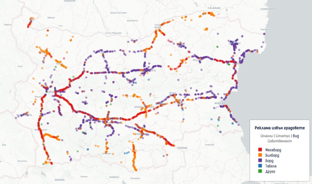
Обърнах се към билбордовете извън населените места на България, защото там виждаме преобладаващо реклама на хазарт и пренасищане. Както и преди, направих карта, която показва различни аспекти на проблема. Ще опиша методологията и какво показва по-късно. Ще започнем с проблемите, за които научих.
Билбордовете извън населените места, а в някои случаи и в тях, следва да отговарят на Наредбата за специално използване на пътищата. Чл. 13 на тази наредба описва как се изграждат и пускат в експлоатация тези съоръжения. На практика фирмите плащат такса и минават многостъпков процес на одобрение при Агенция пътна инфраструктура. Няма значение дали билбордът ще е на частна, общинска или държавна земя – АПИ трябва да одобри и прибере такса, тъй като е край пътя. Същото се отнася впрочем и за бензиностанциите и крайпътните заведения.
Тук се сблъскваме с първото масово нарушение. Чл. 56 на Законът за устройството на територията позволява да се слагат такива преместваеми обекти, но ясно посочва, че разрешение за това може да се дава единствено от общината. Наредбата, по която оперира АПИ, сама споменава ЗУТ, не може да отмени закон и не дава право на АПИ да издава разрешителни за строеж. Всеки един от тези междуградски билбордове освен разрешение за специално ползване от АПИ следва да има и разрешение за поставяне от съответната община по проект.
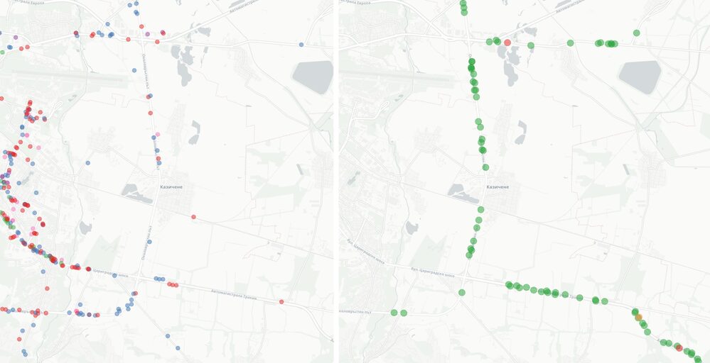
Не открих нито едно разрешение за поставяне на билбордовете в данните на АПИ. Най-лесно беше да се провери в София, където Столична община отговаря за издаването на такива в началото на магистралите. В други общини беше значително по-трудно като повечето въобще не публикуват тези документи. Всички са задължени да ги качват в публичния регистър по ЗУТ. Наредба по него беше пусната най-накрая за обществено обсъждане от служебния кабинет на Гюров и от месеци чака един подпис от министър Шишков. Този регистър ще позволи лесно да се провери законността на всички тези и много други обекти и строежи. Именно това е и причината да беше бавен с години и да се отлага отново и при кабинета на Радев.
Вторият проблем са търговете. Не може да се използва държавна или общинска земя без да е проведен търг. Пътищата на страната са на държавна земя, а мнозинството от билбордовете са в същите имоти или на съседни общински. АПИ не е собственик на тази земя и няма право да я отдава. Това следва да прави областните управители или в случая на общинската земя – търгове към общината. Не открих в публичната информация за търгове нещо свързано с тези билбордове.
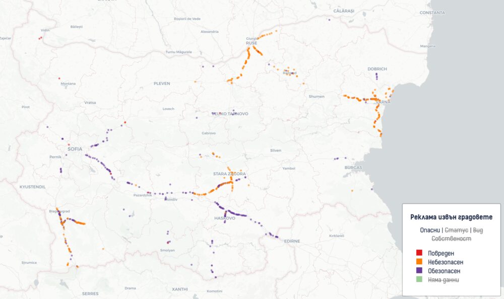
В данните на АПИ открих информация за местоположението и състоянието на 3783 билборда. Към средата на август 11 от тях са повредени. 369 или почти 10% са опасни, но необезопасени. Още 367 са обезопасени. Необезопасените са предимно около Стара Загора, Русе, Благоевград и Варна. Отговорност за това би следвало да е на собствениците и АПИ, а не на общините, които както описах по-горе изглежда не са включени в процеса.
102 или 2.6% са с изтекло или прекратено разрешение от АПИ. При 55 или 1.5% са намерени несъответствия с наредбата като недостатъчно отстояние от възли, пътя или един от друг. Към средата на август във фаза на проектиране са били 23 нови билборда.
12% от рекламите са мегабордове – онези най-големите на високи пилони. 27% са големи билбордове. 56% са малки билбордове, а останалото са табели и други видове реклама.
Чл. 16, ал. 4 от НСПП определя, че срокът за разрешението за специално ползване е 10 г. Това е различно от разрешение за строеж или поставяне, срокът на които се различава. В София, например, е 5 г. В данните на АПИ има дати на такова разрешение за 3600 обекта. Тук виждате разпределението им по години.
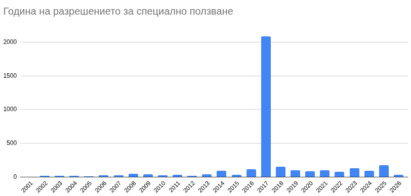
От тях е видно, че огромна част са издадени 2017 г. Всъщност, 61% от разрешенията за всички билбордове извън градовете изтичат до края на 2027 г. Интересното е, че още 12.5% са по-стари и би следвало вече да са изтекли. Само 20% тях обаче са отбелязани като такива. Това значи, че вероятно договорите им са подновени без да е отразено изрично в данните.
Това прави 2027-ма особено важна, защото позволява сериозно намаление на специалното използване на междуградските пътища и магистралите по този начин. Предвид какво знаем за АПИ, интересите и влиянието на хазартния бизнес, вероятно може да очакваме сериозно преразпределяне на пазара на билбордове извън градовете. Тук не трябва да забравяме и ролята на фирмите опериращи билбордове из страната в предизборни кампании – те са сред основните фактори в такива кампании и не са регулирани от ЦИК за разлика от електронните медии – нито като достъпност, равна представителство или дори цена и произход на средствата. Видяхме го ясно при последните парламентарни избори когато огромна част от билбордовете извън градовете бяха обсипани с послания именно на Радев, финансирането за което така и не беше осветено. Всякакви действия в посока регулиране на този бизнес неизбежно следва да се гледа и през тази призма.
От данните на АПИ е изключително трудно да се прецени кой оперира различните билбордове. Има множество свързани фирми, някои са вече преименувани или закрити. Заради грешки в данните като изписване на имена на фирми и ЕИК се наложи да проверя и поправя 10% от записите. Дори тогава беше трудно да се прецени чии са всъщност рекламните обекти.
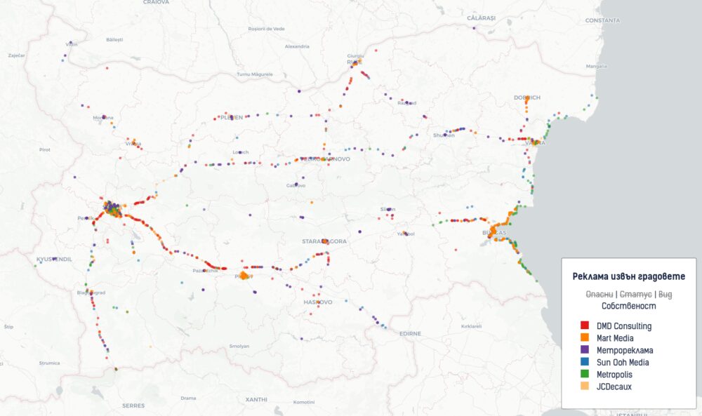
Затова се обърнах към самите компании и какви рекламни площи продават. Събрах данни за шестте най-големи, за които има публична информация. DMD Consulting, Mart Media, Метрореклама, Sun Ooh Media, Metropolis и JCDecaux. Не успях да свържа данните им с тези на АПИ тъй като нямат общи идентификатори и координатите в много случаи не съвпадат. Затова на картата се зареждат като отделен набор от данни.
Ще видите също на картата, че се показват билбордове на тези фирми, които са в градове. Успях да разгранича кои са в населени места и кои са извън. Оставих всички на картата, за да стане видимо присъствието и това разграничение. По публичните данни DMD, например, има 227 билборда и всички са извън градовете. Аналогично изглежда е положението със Sun Ooh Media с 116 билборда. Половината от 381-те билборда на Mart Media са извън градовете, също както 22% от 701-те билборда на Метрореклама и 26% от 311 билборда на Metropolis. JCDecaux имат само 18 билборда извън градовете от общо 1233, което прави 1.5%. Само първите пет фирми управляват 20% от билбордовете в страната и то изглежда на местата с най-голям трафик – по магистралите и морето.
В данните на АПИ виждаме разрешенията им за специално използване, също и данни къде са предвидили да позволяват още билбордове. Това са пространства предимно в държавна земя от двете страни на пътища и магистрали. По наредба има изисквания за отстояние 1500 м. от пътни възли на магистрали и 500 м. от кръстовища на други пътища. Виждаме обаче на картата им, че са отбелязали такива места за бъдеща реклама включително вътре в самите пътни възли. Както споменах по-горе, има и доста изградени вече билбордове, които не отговарят на тези изисквания.
Общата дължина на тези пространства е 62504 км. В това число включваме отсечка и от двете страни на пътя. Би следвало билбордовете да са през 300 метра на магистрали и 200 метра на други пътища, но нека приемем 500 м. отстояние като консервативна оценка. Това означава, че ако рекламният бранш има финансов стимул, би имал възможността да изгради 125 хиляди билборда в страната. Това число изглежда невероятно, но при сегашната процедура и условия на АПИ е не само реалистично и дори консервативно като оценка.
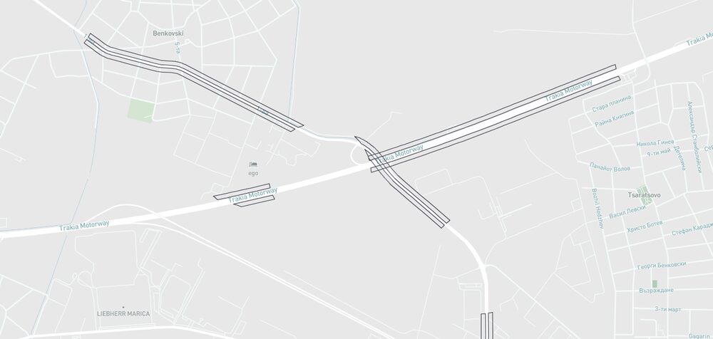
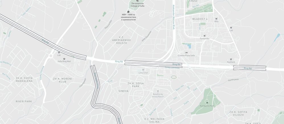
Към този момент имаме данни за 3783 билборда, което прави 3% от тази оценка. Вече ги виждаме на всеки ъгъл по пътищата на страната и дори да стигнем до 10% от разрешеното по наредба. Това означава три пъти повече реклама, разсейване на пътя и почти само хазарт пред очите на пътуващите.
Тук пак трябва да напомня, че АПИ няма право да дава разрешение за строеж нито на 125 хиляди, нито на 3 хиляди билборда. Те могат да позволят само да са до пътя. Разрешението за поставяне или строеж може да се издаде единствено и само от общините. Ако се спази това правило, почти 3800 билборда из страната трябва да се демонтират ведната и да се започне процес отначало всяка община в територията си да ги одобрява.
Данните на АПИ взех от публичния ГИС сървър. Там има още много информация, включително указателни табели, крайпътни обекти и самата пътна мрежа. За рекламните съоръжения и местата за бъдещи такива има два отделни масива. Единият е този показан на тяхната карта, данните от които разглеждам тук. Другият има доста повече данни, които изглежда обаче са архивни и не мога да потвърдя като точност.
Като цяло проблемът с качеството на данните съществува и тук. Информацията се обновява на ръка, което е трудоемко и води до грешки. Обсъждах това в статиите ми за външната реклама на София и изследването на свлачища в страната. В записите за тези билбордове има доста информация, включително бележки за предишни собственици. Споменах по-горе обаче, че имената им са изписвани по няколко различни начини, а ЕИК номерата липсваха или бяха сгрешени в 10% от записите. Поправих ги на ръка като оставих данните където фирма подписала течащ договор за билборд е вече затворена. В такива случаи се оказа, че често билбордовете са купени от друга фирма поела контрола над тях и изглежда АПИ не е обновила новото обстоятелство.
Друг проблем, който открих, са около 50-тина ЕГН-та на частни лица, собственици на фирми или други. Поне 60 от билбордовете са изградени от частни лица, а не фирми по данни на АПИ. Има и много малки фирми, които са направили такива в имотите си или в конкретен район. Всички тези над 3700 билборда се притежават от 685 юридически лица. Това е поне според собствените данни на АПИ, което може би значи, че толкова са подписали договор. Възможно е и често срещам, че след това са препродавани на някой от големите оператори.
Всичко написано до тук като изводи и статистика се базира на собствените данни на АПИ. Както с други карти и анализи, които съм правил, те са толкова точни, колкото самата агенция създава информацията си. Доколкото е видно, че само част от полетата в ГИС сървъра им са видими на публичния портал, може да предположим, че останалото е предимно за вътрешна употреба и представлява поглед над оперативната им дейност. Ако това предположение е вярно, то изводите тук отразяват директно това, което АПИ знае за билбордовете в страната.
Данните за собствеността взех от портали за продажба на рекламни пространства и посредници. Такива далеч не са достъпни за всички оператори на билбордове, затова не мога да твърдя, че картата предоставя представителна извадка в тази категория. Показва обаче добре разпределението на обекти в и извън градовете и как има фирми представени в различни райони или предимно извън градовете или в тях. Ако са ви известни други такива фирми и масиви от данни, изпратете ми ги и ще се опитам да ги добавя.
Местата, където АПИ предвижда, че може да се поставят реклами, са също достъпни на портала на АПИ. Поради огромният обем данни обаче не са налични все още на картата. Ще обновя тази статия като успея да ги добавя така, че да е разбираемо.
Картата, в която събрах данните, е в стандартният формат на всичко, което правя в последните години. Горе вляво има бутони за обща информация, смяна на базов слой със сателитни снимки от Google и фокусиране на картата върху собственото местоположение.
При натискане върху някой билборд се показва подробна информация за него. При данните от АПИ тази информация е разделена на три раздела – общи данни за статус, опасност, собственик и площ, след това подробни данни за разрешението и възможни несъответствия с наредбата и накрая бележки и информация кога е създаден записът. Втори и трети раздел се отварят като натиснете на заглавията. Когато разглеждате собствеността се показва наличната информация за билбордовете според каквото е публично достъпно.
Легендата показва начини на категоризиране и съответните категории. Натискане върху вида категории сменя цветовете на картата според категоризацията. Първите три са от данните на АПИ. При изгледа за собственост се сменят данните към агрегираните от публични източници. Когато натиснете някоя категория се показва само тях изключвайки останалите. За да включите други към този изглед натиснете тях. Когато остане една да бъде скрита се връща изходното състояние показвайки всички.
Картата може да разгледате тук или да я отворите на цял екран.
Имаше много запитвания дали мога да направя карта подобна на тази за София и за други градове. Споменах по-горе, че разрешенията за поставяне са скрити в много общини. Задължени са да ги публикуват, но наредбата за регистъра по ЗУТ се бави. Повечето нямат и регистър на рекламните обекти както в София, който макар и неточен все пак съществува. Данните за собствеността от самите оператори и посредници помага в тази насока и за следващата статия в поредицата ще започна работа по този масив от данни. Ако имате още източници, които не виждате или идеи как може да се агрегира тази информация, ще се радвам да споделите в коментарите.
Както обещах преди седмица, в тази статия се концентрираме върху билбордовете извън градовете. Не е тайна, че повечето от тях са заети с реклама на хазарт. Тук НАП има важна роля, която не изпълнява. Едно от извиненията, които са давали в интервюта, отговори по ЗДОИ и включително на депутати е, че нямат данни къде и колко са тези билбордове. Наивно е да се смята, че това извинение е нещо повече от прикриване на желанието за бездействие и обслужване на интересите както на операторите на билбордове, така и на хазартния бизнес. Ако наистина липсата на данни е пречка. На драго сърце бих предоставил всичко, което съм събрал.
Както в предишната си статия, така и сега поставих под съмнение законността на голяма част от рекламните площи. Всъщност, на база публично достъпната информация може да твърдим, че почти няма билборд извън градовете, който да е законен. АПИ е иззела функции по ЗУТ и изглежда няма община, която да им се опълчи. Премахването на незаконни билбордове и преместваеми обекти е проблем като цяло – скъпо начинание е усложнено допълнително от АПК и бавните и непостоянни административни съдилища. Отделно държавата и самите общини следва да правят търгове за поставяне на такива обекти. Това не се случва и отново е оставен АПИ да вършее.

Докато работих по тази карта в последните дни излезе слух, че кабинетът на Радев обмисля забрана на рекламата на хазарт в градовете. Това остава рекламата им съвсем да залее билбордовете, които изброявам горе. Такава идея е била прокарвана и в миналото без резултат по разбираеми причини. Данните на АПИ и тези за собствеността показват, че това обслужва точно определени бизнес интереси, както и че ще засили стимулът да се изграждат още хиляди до десетки хиляди билбордове на всеки 200 до 300 метра междуградски път. Промяната, ако наистина сериозно се обмисля, е несъмнено лобистка и се прави точно в момент, в който пазарът се преразпределя.
По-важното обаче е, че подобна мярка би била дим пред реалният проблем – огромната щета за обществото и печалби, които този бизнес прави. Несъмнено има постъпления за бюджета, които далеч не са дори реалните суми, които следва да плащат. Дори така те са на практика данък уязвимост и данък бедност. Заедно с бързите кредити, телефонните измами, цигарите и вейповете хазартът има най-голяма роля в разрушаването на финансовата стабилност и живота на стотици хиляди български семейства.
Петте процента ограничение за рекламите беше приемлив компромис. Предвид невъзможността, а явно нежеланието да се съблюдава и санкционират нарушителите, единственото възможно решение е пълна забрана за реклама на хазарт. Всичко останало е нищо повече от обслужване на лобистки интереси.
Post Syndicated from corbet original https://lwn.net/Articles/1089251/
The open-source world has been struggling for a few years now to understand
how to approach large language models (LLMs) and the licensing applied to
them. What constitutes “freedom” with respect to a black box filled with
numerical weights? The process taken by the Open Source Initiative (OSI)
in the development of its Open AI
Definition was controversial at best, as was its output. Now, the
Linux Foundation’s Mike Dolan has brought
a new license to the OSI for approval. It is called the OpenMDW (“Open
Model, Data, and Weights”), and it aims to clarify licensing for the
distribution of LLMs and related materials, but consensus is proving hard
to find for this license as well.
Post Syndicated from jzb original https://lwn.net/Articles/1089999/
Security updates have been issued by AlmaLinux (ansible-core and pcp), Debian (chromium, libgit2, python-httplib2, and sabnzbdplus), Fedora (dokuwiki, domoticz, dotnet10.0, dotnet8.0, dotnet9.0, firefox, i2c-display, libgit2, lyx, ntpsec, openssh, perl-DBI, php-phpseclib3, python-alembic, python-asyncmy, python-sqlalchemy, python3.13, roundcubemail, trafficserver, wireshark, and wordpress), Red Hat (compat-openssl10, compat-openssl11, fence-agents, gnutls, kernel, kernel-rt, libarchive, libreswan, multiple packages, openssl, python-idna, python-pillow, qemu-kvm, resource-agents, rh-podman-desktop, ruby, unbound, and vim), SUSE (buildah, chromium, container-suseconnect, containerd, cosign, ctop, docker, firefox, forgejo-cli, gitea-tea, go1.25, go1.26, helm, kubernetes, kubernetes-old, kubevirt1.8, podman, python-pytest-html, python-unearth, python311, python313, rootlesskit, and rsync), and Ubuntu (linux, linux-aws, linux-aws-5.4, linux-azure, linux-bluefield, linux-fips,
linux-gcp, linux-gcp-5.4, linux-hwe-5.4, linux-ibm, linux-ibm-5.4,
linux-iot, linux-oracle, linux-raspi, linux-raspi-5.4, linux-xilinx-zynqmp, linux, linux-aws, linux-aws-7.0, linux-ibm, linux-oem-7.0, linux-raspi,
linux-realtime, linux, linux-aws, linux-aws-fips, linux-azure-fips, linux-gkeop,
linux-ibm-5.15, linux-intel-iot-realtime, linux-intel-iotg,
linux-intel-iotg-5.15, linux-kvm, linux-nvidia, linux-nvidia-tegra,
linux-nvidia-tegra-5.15, linux-oracle, linux-oracle-5.15, linux-realtime,
linux-xilinx-zynqmp, linux, linux-aws, linux-kvm, linux-lts-xenial, linux-aws-6.8, linux-azure-5.15, linux-gcp, linux-gcp-fips, linux-hwe-5.15,
linux-lowlatency-hwe-5.15, linux-gcp, linux-gcp-4.15, linux-gcp-fips, linux-gcp, linux-gke, linux-gke, linux-lowlatency, linux-lowlatency-hwe-6.8, linux-hwe-6.8, linux-nvidia, linux-nvidia-7.0, linux-nvidia-bos, linux-raspi, linux-raspi-realtime, netty, postgresql-14, postgresql-16, postgresql-18, vim, and wget).