Patrick Garrity of VulnCheck has written a blog
post that looks at vulnerabilities found by Anthropic’s Project Glasswing since it
launched on April 7, and finds it wanting:
Of the 37,966 findings Anthropic reports, only 7,349 (19.4%) have been made
public. Just 217 of those have been marked fixed. The more glaring number is
that 4.4% (1,654) of the project’s findings have already been marked as
duplicates, 7.5x more duplicates than fixes. On top of that, 419 findings have
been withdrawn. It seems odd that the ledger now claims a 94.2% true positive
rate, up from 90.8% at launch, when more findings have been withdrawn or marked
as duplicates than fixed, likely a feedback loop missing to the triage rates
listed as “True Positives”.
[…] AI is a valuable tool for finding vulnerabilities, and I’m not
discounting that. But seven months in, the evidence still doesn’t match the
launch narrative. The CVEs are a sliver of this year’s total, almost none are
being exploited, fixes have stalled while duplicates and withdrawals pile up,
and the triage burden is shifting onto the open source maintainers Glasswing
promised to help. The receipts keep coming in. They still don’t reconcile.
A cloud data lake is a scalable, low-cost place to store data from many different sources. Over the years, data lakes built on Amazon Simple Storage Service (Amazon S3) have become a common home for enterprise data, used by teams who query it for analytics and machine learning. However, data lakes have historically made it hard to update and delete records, keep transactions isolated, and handle concurrent changes safely. Open table formats such as Apache Hudi, Delta Lake, and Apache Iceberg were created to solve these problems. They add ACID transactions and row-level updates and delete, along with snapshot history and schema enforcement that make data lakes easier to audit and govern.
As organizations’ data architectures mature and evolve, the need to migrate between these table formats becomes increasingly common. This transition is often driven by changing requirements, performance considerations, or the desire to use newer features. Among these migrations, the shift from Apache Hudi to Apache Iceberg has gained particular attention, as organizations seek to capitalize on Iceberg’s modern architecture and advanced capabilities.
In this post, we show how to convert Apache Hudi tables to Apache Iceberg, using a Jupyter notebook running on AWS Glue 5.1 interactive sessions.
Benefits of migration to Iceberg
Enhanced partition evolution
Iceberg supports dynamic changes to partitioning schemes without requiring complete data rewrites. This capability is valuable in evolving data environments where query patterns change over time. You can adjust your partitioning strategy to optimize performance, reducing the operational overhead traditionally associated with such changes. Your data lake can adapt to changing business requirements without costly reorganization efforts.
Hidden partitioning
In addition to standard partitioning on an existing column, Iceberg supports hidden partitioning, which decouples the physical partition layout from the columns that queries filter on. The table specification declares a partition transform, which is a rule that tells Iceberg how to derive the partition value from a source column, such as a time bucket or a hash of the column value. The transform is defined once at the table level, and Iceberg applies it automatically on every write. This removes a long-standing source of friction on both sides of the table: writers no longer need to extract and maintain a separate partition column alongside the real one at ingestion time, and queries no longer need to carry an extra predicate on that derived column to get good performance.
Openness with the Iceberg REST Catalog
The Iceberg REST Catalog specification defines a standard HTTP protocol for catalog operations. Any engine that speaks the protocol can talk to any catalog that implements it, without a catalog-specific client library or implementation JAR on the class path. Integration moves from a code and dependency problem to a configuration problem, making Iceberg a strong fit for multi-engine data architectures.
Deep integration with AWS services
Iceberg has native integration across the AWS analytics ecosystem. Amazon Athena, Amazon Redshift, Amazon EMR, and AWS Glue all read and write Iceberg tables directly. The AWS Glue Data Catalog provides catalog and metadata management for these tables, and Amazon SageMaker builds on the same open Lakehouse foundation, letting analytics and artificial intelligence and machine learning (AI/ML) workloads share a single copy of data across Amazon S3 data lakes (including Amazon S3 Tables), with SageMaker Feature Store supporting an Iceberg offline store for faster training dataset extraction. On the ingestion side, Amazon Data Firehose delivers data into Iceberg tables from sources such as Direct PUT, Amazon Kinesis Data Streams, Amazon Managed Streaming for Apache Kafka (Amazon MSK), Amazon CloudWatch Logs, and AWS IoT, with optional on-the-fly record transformation by using AWS Lambda. No-code Streaming Tables map a single Kinesis Data Streams stream or a single Amazon MSK (Express brokers) Kafka topic to a single Amazon S3 Tables Iceberg table, with the target table auto-created and partitioning configured on the delivery channel.
AWS managed features
AWS provides managed capabilities specifically designed for Iceberg. These managed features reduce operational overhead while maintaining performance and cost efficiency, so teams can focus on deriving insights rather than managing infrastructure.
AWS Glue Iceberg table optimizer – Automated compaction, snapshot management, and orphan file cleanup without manual intervention on Iceberg tables in General S3 buckets.
Amazon S3 Tables – Fully managed Iceberg tables with automatic optimization and maintenance.
Zero-ETL integration – Managed, incremental replication from Amazon DynamoDB and third-party enterprise applications such as Salesforce, SAP, ServiceNow, and Zendesk into Iceberg tables in Amazon S3 (self-managed or Amazon S3 Tables), with no custom pipeline or connector code to maintain. Source changes are applied incrementally, so the target stays in sync without full reloads.
Iceberg materialized views – SQL-defined views materialized as native Iceberg tables, refreshed on an automatic schedule and incrementally when the source tables allow it, with change detection handled for you. Well suited to consumption-layer tables that feed dashboards, APIs, and downstream pipelines, since the work shifts from query time to the managed refresh.
These benefits make Apache Iceberg a strong choice for modern data lake implementations, offering advantages in performance, manageability, and scalability compared to traditional table formats.
In the context of migrating data to Apache Iceberg, two primary approaches exist: in-place migration and full table migration. We previously covered both in the blog post “Migrate an existing data lake to a transactional data lake using Apache Iceberg” which walks through the methodology for traditional Hive-style tables, meaning partitioned Apache Parquet, Apache ORC, or Apache Avro datasets registered in a Hive-compatible catalog. The same two approaches apply when the starting point is an Apache Hudi data lake, which comes in two flavors, Copy-on-Write (CoW) and Merge-on-Read (MoR).
In-place migration
This approach generates fresh Iceberg metadata on top of the existing data files of the source table, without rewriting the data itself. The Parquet files of a Hive, Hudi, or Delta Lake table stay in place, and a new or existing Iceberg table is pointed at them with its own metadata layer. The main advantage is cost and speed: no data rewrite, so the migration is fast and cheap on both compute and storage. The main limitation is that the Iceberg table inherits the source table’s schema, partitioning, and physical file shape (file sizes, row groups, sort order), and none of these can be changed during the migration itself.
Full table migration
In this approach, the data itself is rewritten into a new Iceberg table, typically using a writeTo() call or a CREATE TABLE AS SELECT (CTAS) statement. It works for any source an engine can read from (Hive, Hudi, Delta Lake, relational databases, and others), and because the data is being rewritten anyway, the migration step is also where you can reshape it: change the schema, apply Iceberg hidden partitioning, resort the data for pruning, and target larger file sizes than the source has. The trade-offs are cost, time, and storage: higher compute spend, longer migration, and the dataset is effectively stored twice (source and target) until the migration completes, and the source is retired. For large historical tables, a single CTAS is usually impractical, so the common pattern is to seed the table with a small CTAS and then run INSERT INTO ... SELECT partition by partition, parallelizing and checkpointing across batches.
In this post we work through both approaches end-to-end. We first create a sample Hudi event table in each flavor, CoW and MoR, then migrate them in place to Iceberg using two techniques, the Spark Iceberg add_files procedure and the Apache XTable sync tool, covering the considerations and prerequisites of each. Finally, we walk through the full table migration path, where the source data is rewritten into a new Iceberg table from scratch.
Solution overview
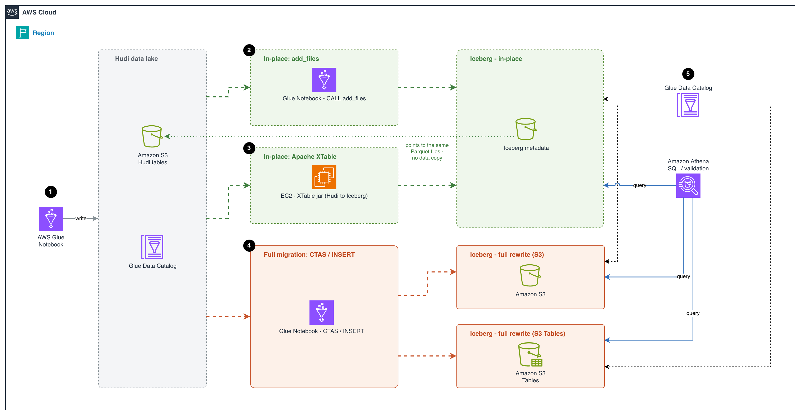
The following diagram illustrates the architecture that you implement through this post.
Figure 1: Migration architecture showing the in-place paths (add_files and Apache XTable) and the full-table paths (CTAS and INSERT) to Amazon S3 and Amazon S3 Tables, all registered in the AWS Glue Data Catalog and queried with Amazon Athena
The workflow consists of the following steps:
An AWS Glue notebook writes the source data as Apache Hudi tables to an Amazon S3 bucket and registers them in the AWS Glue Data Catalog. This creates the existing Hudi data lake that the migration starts from.
The first in-place migration approach uses an AWS Glue notebook to run the Apache Iceberg add_files procedure. The procedure creates Iceberg metadata on top of the Parquet data files already in the Hudi table. The new Iceberg metadata points to the same Parquet files, so no data is copied or rewritten. This makes it a fast, low-cost migration path.
The second in-place migration approach runs Apache XTable on an Amazon Elastic Compute Cloud (Amazon EC2) instance to convert the Hudi table metadata into Iceberg metadata. XTable reads the Hudi commit timeline and creates matching Iceberg metadata that points to the same Parquet files. Both table formats can then share a single copy of the data.
For a full migration, an AWS Glue notebook uses CREATE TABLE AS SELECT (CTAS) or INSERT INTO statements to read the Hudi data and rewrite it as new Iceberg tables. The tables can go in a general purpose S3 bucket or in Amazon S3 Tables. This approach fully separates the new tables from the Hudi source. S3 Tables also handle table maintenance for you, such as compaction and snapshot management.
The AWS Glue Data Catalog registers the Iceberg tables from all three approaches. Users can then use Amazon Athena, a serverless query service, to run SQL queries on these tables and validate the migrated data. Athena enables interactive SQL-based exploration of data directly in Amazon S3 without the need for complex infrastructure management.
Prerequisites
Before getting started, make sure you have the following:
An AWS account with a role that has sufficient access to provision the required resources.
Sign in to the AWS Management Console and open the AWS Glue console.
In the Region selector (top right), choose your preferred working Region.
Choose ETL Jobs in the left pane.
Choose Notebook under Author using an interactive code notebook, select Start fresh, choose your IAM role, and choose Create notebook.
After a minute, the Jupyter notebook editor appears. Clear all the default cells.
Create Hudi Copy-on-Write (CoW) and Merge-on-Read (MoR) sample event tables
This notebook creates Hudi tables using both Copy-on-Write (CoW) and Merge-on-Read (MoR) table types with sample events. We perform inserts, updates, and deletes, then inspect the underlying file structures to understand the key differences:
CoW: an update or delete fully rewrites every base Parquet file that contains an impacted row, producing a new file slice in the file group. Reads are cheap, and writes amplify with the fraction of files touched.
MoR: an update or delete is appended to an Avro log file alongside the base file instead of rewriting the base, and base + logs are merged at read time (or compacted into a new base file later). Cheaper writes. Costlier reads until compaction.
Execute the first cell with the following configuration to set up the Spark session with Hudi and Iceberg support:
Initialize the session and configuration. Update the bucket_name, db_name and region variables with your configurations. Reusable helper – list_table_files(table_name, label="", verbose=False) renders a table’s S3 layout as a directory tree so you can SEE how CLEAN, COMPACT and add_files change the files underneath. It is reused before/after each of those steps instead of re-coding the listing.
Code:
# ──────────────────────────────────────────────
# Source Hudi tables
# ──────────────────────────────────────────────
hudi_events_cow_table = "events_hudi_cow" # Copy-on-Write source
hudi_events_mor_table = "events_hudi_mor" # Merge-on-Read source
# ──────────────────────────────────────────────
# In-place migration targets (add_files/xtable)
# ──────────────────────────────────────────────
iceberg_cow_inplace = "events_iceberg_cow_inplace"
iceberg_mor_inplace = "events_iceberg_mor_inplace"
iceberg_cow_xtable = "events_hudi_cow_iceberg_xtable"
iceberg_mor_xtable = "events_hudi_mor_iceberg_xtable"
# ──────────────────────────────────────────────
# Full table (shadow) migration targets
# ──────────────────────────────────────────────
iceberg_cow_full_ctas = "events_iceberg_cow_full_ctas"
iceberg_cow_full_create_insert = "events_iceberg_cow_full_create_insert"
iceberg_mor_full_ctas = "events_iceberg_mor_full_ctas"
iceberg_mor_full_create_insert = "events_iceberg_mor_full_create_insert"
# ──────────────────────────────────────────────
# Infrastructure
# ──────────────────────────────────────────────
bucket_name = "demoblogiceberg-bdb5001" # S3 bucket for data
db_name = "hudi_to_iceberg_blog" # Glue Data Catalog database
region = "us-east-1"
# Create the Glue Data Catalog database
spark.sql(f"""
CREATE DATABASE IF NOT EXISTS {db_name}
LOCATION 's3://{bucket_name}/{db_name}'
""")
# Reusable helper —list_table_files()(S3 layout tree)
import boto3
s3 = boto3.client('s3', region_name=region)
# File/folder annotations keyed by classifier result
_NOTES = {
"hoodie_dir": "<-- Hudi metadata (timeline, schema, indexes)",
"hoodie_mdt": "<-- Hudi metadata table (internal index & stats, MoR)",
"hoodie_files": "<-- file listing index",
"hoodie_cstats":"<-- column-level min/max/null stats",
"hoodie_ridx": "<-- record-key -> file-group mapping",
"ice_meta_dir": "<-- Iceberg metadata layer (metadata.json, manifest lists, manifests)",
"ice_data_dir": "<-- Iceberg data layer (base Parquet files)",
"base": "<-- base Parquet file",
"log": "<-- Hudi delta log file (MoR update, uncompacted)",
"part_meta": "<-- Hudi partition marker",
"metadata_json":"<-- Iceberg table metadata (schema, snapshots)",
"manifest_list":"<-- Iceberg manifest list (snapshot -> manifests)",
"manifest": "<-- Iceberg manifest (lists data files)",
"props": "<-- table configuration & schema",
}
# Fixed-path annotations for metadata directories
_DIR_KIND = {
".hoodie": "hoodie_dir", ".hoodie/metadata": "hoodie_mdt",
".hoodie/metadata/files": "hoodie_files",
".hoodie/metadata/column_stats": "hoodie_cstats",
".hoodie/metadata/record_index": "hoodie_ridx",
"metadata": "ice_meta_dir", "data": "ice_data_dir",
}
def _fmt_size(n):
"""Human-readable byte size."""
for u in ("B", "KB", "MB", "GB", "TB"):
if n < 1024 or u == "TB":
return f"{n:,.0f} {u}" if u == "B" else f"{n:,.1f} {u}"
n /= 1024.0
def _leaf_kind(name):
"""Classify a leaf file by name -> annotation key / count bucket."""
if ".log." in name: return "log"
if name.startswith(".hoodie_partition_metadata"): return "part_meta"
if name == "hoodie.properties": return "props"
if name.endswith(".metadata.json"): return "metadata_json"
if name.startswith("snap-") and name.endswith(".avro"): return "manifest_list"
if name.endswith(".avro"): return "manifest"
if name.endswith(".parquet"): return "base"
return ""
def list_table_files(table_name, label="", verbose=False, max_depth=2, max_children=2):
"""Render a Hudi/Iceberg table's S3 layout as an annotated directory tree.
Teaching view for CLEAN/COMPACT/add_files: multiple base files in a partition
= stale file slices; .log.* = uncompacted MoR updates. The large Hudi .hoodie/
is summarized (depth/width capped); Iceberg metadata/ and data partitions show
in full. verbose=True expands everything.
"""
prefix = f"{db_name}/{table_name}/"
header = f"s3://{bucket_name}/{prefix}"
if label:
header += f" [{label}]"
print(header)
in_meta = lambda p: (p.split("/", 1)[0] if p else "") in (".hoodie", "metadata")
capped_meta = lambda p: (p.split("/", 1)[0] if p else "") == ".hoodie"
# ---- gather objects into a nested tree + tally honest counts -----------
root = {"d": {}, "f": []}
n_base = n_log = n_meta = n_other = 0
s_base = s_log = s_meta = 0
has_hudi = has_ice = False
for page in s3.get_paginator("list_objects_v2").paginate(Bucket=bucket_name, Prefix=prefix):
for obj in page.get("Contents", []):
key = obj["Key"].replace(prefix, "")
size = obj["Size"]
if key == "" or key.endswith("/"):
continue # S3 directory marker
parts = key.split("/")
fname, top = parts[-1], parts[0]
if top == ".hoodie": has_hudi = True
if top == "metadata": has_ice = True
# files inside a metadata folder count ONLY as metadata
if top in (".hoodie", "metadata"):
n_meta += 1; s_meta += size
elif ".log." in fname:
n_log += 1; s_log += size
elif fname.endswith(".parquet"):
n_base += 1; s_base += size
elif fname.startswith(".hoodie"):
n_meta += 1; s_meta += size; has_hudi = True
else:
n_other += 1
node = root
for part in parts[:-1]:
node = node["d"].setdefault(part, {"d": {}, "f": []})
node["f"].append((fname, size))
# ---- helpers -----------------------------------------------------------
def count_all(node):
return len(node["f"]) + sum(count_all(c) for c in node["d"].values())
def collapse(node, name, rel):
"""Merge single-child, file-less dir chains (year=/month=/day=)."""
while (len(node["d"]) == 1 and not node["f"] and not in_meta(rel)):
cname, child = next(iter(node["d"].items()))
crel = f"{rel}/{cname}"
if in_meta(crel): break
name, rel, node = f"{name}/{cname}", crel, child
return name, rel, node
def line(indent, branch, text, note, width):
s = f"{indent}{branch}{text}"
return f"{s:<{width}} {note}" if note else s
def render(node, rel, indent, depth):
entries = ([("d", n, c) for n, c in sorted(node["d"].items())]
+ [("f", n, sz) for n, sz in sorted(node["f"], key=lambda f: (".log." in f[0], f[0]))])
cap = (not verbose) and capped_meta(rel) and len(entries) > max_children
shown = entries[:max_children] if cap else entries
hidden = len(entries) - len(shown)
for i, item in enumerate(shown):
last = (i == len(shown) - 1) and hidden == 0
branch = "└── " if last else "├── "
sub = indent + (" " if last else "│ ")
if item[0] == "d":
_, name, child = item
disp, erel, enode = collapse(child, name, f"{rel}/{name}" if rel else name)
note = _NOTES.get(_DIR_KIND.get(erel, ""), "")
cnt = f" ({count_all(enode)} obj)" if (in_meta(erel) or erel in _DIR_KIND) else ""
print(line(indent, branch, f"{disp}/{cnt}", note, 60))
if (not verbose) and capped_meta(erel) and depth + 1 > max_depth:
inner = count_all(enode)
if inner:
print(f"{sub}└── … ({inner} objects, use verbose=True)")
else:
render(enode, erel, sub, depth + 1)
else:
_, name, size = item
note = _NOTES.get(_leaf_kind(name), "")
print(line(indent, branch, f"{name} ({_fmt_size(size)})", note, 72))
if hidden:
print(f"{indent}└── … (+{hidden} more)")
render(root, "", "", 0)
# ---- per-partition slice note (Hudi concept; skip metadata & Iceberg data/) ----
def slices(node, rel):
top = rel.split("/", 1)[0] if rel else ""
if top in (".hoodie", "metadata", "data"):
return
nb = sum(1 for f, _ in node["f"] if f.endswith(".parquet"))
nl = sum(1 for f, _ in node["f"] if ".log." in f)
if nb > 1:
print(f" note: {rel}/ has {nb} base files -> multiple file slices (stale versions)")
elif nb == 1 and nl:
print(f" note: {rel}/ has 1 base + {nl} log file(s) -> uncompacted MoR updates")
for n, c in node["d"].items():
slices(c, f"{rel}/{n}" if rel else n)
slices(root, "")
# ---- in-place migration note -------------------------------------------
if has_ice and "data" not in root["d"] and n_base == 0:
print(" note: Iceberg metadata/ present but no local data/ folder")
print(" -> in-place migration: data files remain registered in place at the source (Hudi) location; no data copied")
# ---- summary -----------------------------------------------------------
total = n_base + n_log + n_meta + n_other
print(
f"SUMMARY: {n_base} base · {n_log} log · {n_meta} meta"
+ (f" · {n_other} other" if n_other else "")
+ f" · {total} files · {_fmt_size(s_base + s_log + s_meta)}"
)
print(f" .hoodie/: {'present' if has_hudi else 'none'} metadata/ (Iceberg): {'present' if has_ice else 'none'}")
print()
Sample event data
We use a website clickstream events dataset, partitioned by year/month/day – a realistic pattern for event-driven architectures.
Note: In this example, we create the table with a preCombineField, which flips the default write operation of INSERT INTO from insert to upsert. You can override it explicitly with hoodie.spark.sql.insert.into.operation when you need a different behavior.
CoW table: create, upsert, and delete
We create a Hudi CoW table, insert records, apply an upsert, and delete a record, then inspect how the files change.
Create the Hudi CoW events table
Code:
spark.sql(f"""
CREATE TABLE {db_name}.{hudi_events_cow_table} (
event_id STRING,
user_id STRING,
event_type STRING,
event_timestamp TIMESTAMP,
page_url STRING,
year INT,
month INT,
day INT
)
USING HUDI
OPTIONS (
type = 'cow',
primaryKey = 'event_id',
preCombineField = 'event_timestamp'
)
PARTITIONED BY (year, month, day)
LOCATION 's3://{bucket_name}/{db_name}/{hudi_events_cow_table}/'
""")
print("=== COW Table (events_hudi_cow) ===")
spark.sql(f"SELECT event_id, user_id, event_type, event_timestamp, page_url, year, month, day FROM {db_name}.{hudi_events_cow_table} ORDER BY event_id").show(truncate=False)
print("\n=== MOR Table (events_hudi_mor) ===")
spark.sql(f"SELECT event_id, user_id, event_type, event_timestamp, page_url, year, month, day FROM {db_name}.{hudi_events_mor_table} ORDER BY event_id").show(truncate=False)
Migrate Hudi tables to Iceberg with in-place migration
In-place migration keeps the original Parquet data files where they are and only builds Iceberg metadata on top of them. There is no rewrite of the underlying data, which makes the migration fast and inexpensive even on large tables. Two tools cover the common cases on AWS:
add_files (Iceberg built-in procedure). A Spark procedure shipped with Apache Iceberg that registers existing Parquet files into an Iceberg table by writing the corresponding manifests, without rewriting the data. It runs as a Spark job in which the source table’s partitions are distributed across Spark tasks, so file listing and column-statistics gathering happen in parallel on the cluster.
Apache XTable (incubating). An open-source cross-format translation tool that can read the metadata of one lakehouse format (Hudi, Delta, or Iceberg) and write out the equivalent metadata for another, pointing at the same underlying Parquet files. XTable can run once to produce the initial Iceberg metadata, or run on a schedule to keep the Iceberg view continuously in sync with ongoing writes to the Hudi table.
Choosing between add_files and Apache XTable for in-place migration
When planning an in-place migration, it is important to understand the strengths of each approach:
add_files is best suited for a one-time migration. It registers existing Hudi Parquet files into an Iceberg table in a single operation. After the migration is complete, the source Hudi table and target Iceberg table are independent, and any subsequent changes to the Hudi table are not reflected in Iceberg.
Apache XTable supports both an initial one-time conversion and ongoing incremental synchronization. This makes it ideal for transition periods where you need to keep both the source Hudi tables and the target Iceberg tables in sync while downstream consumers gradually migrate to Iceberg. After all workloads have been cut over, you can stop the sync process and decommission the Hudi tables.
Important notes
add_files/XTable register existing Parquet files as-is, so they rely on the column names baked into each file. Added and dropped columns are safe, but if the source table was renamed any column during its lifecycle, files written before the rename still hold the old name and reads against the new name return NULL for them. For tables with a history of column renames, prefer a full migration instead.
Iceberg version and column statistics (in-place add_files / snapshot): In Iceberg 1.9.0 through 1.10.0, the add_files and snapshot procedures don’t generate column stats in the Iceberg metadata. The cause is a NameMapping loss in ParquetUtil.footerMetrics. Without those column-level lower/upper bounds and null counts, the migrated Iceberg table loses most of its file-skipping ability at query planning time, which translates into more Parquet files being inspected, higher scan volume, and slower queries, especially for selective filters on non-partition columns. The issue is fixed in the Iceberg 1.10.1 release (#14617). Affected runtimes are AWS Glue 5.1 and Amazon EMR 7.11–7.13. We recommend AWS Glue 6.0+ or Amazon EMR 7.14+ for production migrations.
Shared data files during in-place migration: With both approaches, the in-place migration doesn’t copy data. The resulting Iceberg table points to the same underlying Parquet files as the source Hudi table. This means that until you perform a full cutover to Iceberg, you must avoid destructive operations on the Iceberg table that could delete or modify the shared data files. Specifically:
Don’t drop the Iceberg table with the PURGE option.
Don’t run Iceberg maintenance tasks such as expire_snapshots or remove_orphan_files.
Running any of these before cutover can remove files that the source Hudi table still depends on, leading to data loss. Iceberg exposes a built-in guardrail against this: the gc.enabled table property. When set to false, Iceberg blocks the preceding destructive operations. How you apply this depends on which migration path you choose.
With add_files. Disable garbage collection immediately after the procedure finishes and keep it disabled until you have fully cut over to Iceberg.
Right after add_files:
spark.sql(f"""
ALTER TABLE {db_name}.{table_name}
SET TBLPROPERTIES ('gc.enabled' = 'false');
""")
After Hudi source is retired and the Iceberg table owns its own data, re-enable GC so maintenance can run normally:
spark.sql(f"""
ALTER TABLE {db_name}.{table_name}
SET TBLPROPERTIES ('gc.enabled' = 'true');
""")
With Apache XTable (incremental sync). The gc.enabled = false guardrail is only partially usable here, because XTable’s incremental sync needs GC to be enabled on the Iceberg table to operate normally. A practical pattern is:
Run the initial full XTable sync.
Temporarily set gc.enabled = false to run post-migration validation and consistency checks on the Iceberg table in a safe state.
Set gc.enabled = true again before starting incremental sync and leave it on for the duration of the sync period.
Because the automatic guardrail is off during incremental sync, the burden shifts to operational discipline: as long as XTable is syncing and data files are shared with the Hudi table, don’t run any Iceberg operation that can delete source data files (no DROP TABLE ... PURGE, no expire_snapshots, no remove_orphan_files, no manual object deletion against the shared S3 prefix). Treat the Iceberg table as read-only in terms of file lifecycle until cutover is complete, and Hudi is decommissioned, at which point normal Iceberg maintenance can resume.
Don’t enable the AWS Glue Data Catalog table optimizer before cutover.
Glue-managed Iceberg maintenance (compaction, snapshot retention, orphan file cleanup) will rewrite or delete the Parquet files that the source Hudi table still depends on. Verify that no catalog-level optimizer applies to the migrated table and leave table-level optimization off until cutover is complete.
Prerequisites for in-place migration with add_files. The add_files procedure registers every Parquet file it finds under the source location into the target Iceberg table, with no awareness of Hudi’s file-group versioning. If more than one file version of the same record is present at migration time, each version is registered as a separate row, and the Iceberg table will contain duplicates. The source Hudi table must therefore expose exactly one file version per record before add_files runs:
CoW tables: Run CLEAN to remove old file versions, keeping only the latest Parquet files.
MoR tables: Run COMPACTION (merge delta logs into base Parquet) + CLEAN before calling add_files, since add_files can only register base Parquet files and cannot process Hudi delta log files.
Option 1: Migrate Hudi tables to Iceberg with the add_files Spark procedure
This option uses the Iceberg add_files procedure to register the existing Hudi Parquet files into new Iceberg tables. Run it once per table, after preparing the Hudi table so that only the current file versions remain.
Migrate CoW to Iceberg
We create the target Iceberg table, prepare the Hudi source so that only the current file versions remain, register those files, and validate the result.
Create the target Iceberg table with the same schema
Code:
spark.sql(f"""
CREATE TABLE glue_iceberg.{db_name}.{iceberg_cow_inplace} (
event_id STRING,
user_id STRING,
event_type STRING,
event_timestamp TIMESTAMP,
page_url STRING,
year INT,
month INT,
day INT
)
USING iceberg
PARTITIONED BY (year, month, day)
LOCATION 's3://{bucket_name}/{db_name}/{iceberg_cow_inplace}/'
""")
Run Hudi CLEAN to keep only the latest file versions
Check files listing for the Hudi table before the CLEAN operation:
Code:
list_table_files(hudi_events_cow_table, "COW --- BEFORE CLEAN")
Output:
s3://demoblogiceberg-bdb5001/hudi_to_iceberg_blog/events_hudi_cow/ [COW — BEFORE CLEAN]
├── .hoodie/ (50 obj) <-- Hudi metadata (timeline, schema, indexes)
│ ├── .......trimmed
└── year=2024/month=4/
├── day=1/
│ ├── .hoodie_partition_metadata (96 B) <-- Hudi partition marker
│ ├── 7d187e9a.....20261011152509633.parquet (426.3 KB) <-- base Parquet file
│ └── 7d187e9a.....20261011152403779.parquet (426.4 KB) <-- base Parquet file
├── day=2/
│ ├── .hoodie_partition_metadata (96 B) <-- Hudi partition marker
│ └── e583fe17.....20261011152403779.parquet (426.4 KB) <-- base Parquet file
└── day=3/
├── .hoodie_partition_metadata (96 B) <-- Hudi partition marker
├── eedc1b38.....20261011152509633.parquet (426.3 KB) <-- base Parquet file
├── eedc1b38.....20261011152539102.parquet (426.2 KB) <-- base Parquet file
└── eedc1b38.....20261011152403779.parquet (426.4 KB) <-- base Parquet file
note: year=2024/month=4/day=1/ has 2 base files -> multiple file slices (stale versions)
note: year=2024/month=4/day=3/ has 3 base files -> multiple file slices (stale versions)
SUMMARY: 6 base · 0 log · 53 meta · 59 files · 2.8 MB
.hoodie/: present metadata/ (Iceberg): none
Run the CLEAN operation specifying to keep only the latest file slices:
We can see the Hudi and Iceberg tables reflect the same content:
Code:
print("Source: Hudi COW")
spark.sql(f"SELECT event_id, user_id, event_type, event_timestamp, page_url FROM {db_name}.{hudi_events_cow_table} ORDER BY event_id").show(truncate=False)
print("Target: Iceberg (in-place)")
spark.sql(f"SELECT event_id, user_id, event_type, event_timestamp, page_url FROM glue_iceberg.{db_name}.{iceberg_cow_inplace} ORDER BY event_id").show(truncate=False)
Trigger COMPACTION scheduling on the MoR table with the delta-commit and age thresholds set to their minimum, so any file slice with pending log files is included in the plan and merged back into its base Parquet file.
Execute the previously scheduled compaction plan to merge the pending log files into their base Parquet files. The REQUESTED instant produced by the schedule step transitions to COMPLETED, and the table is left with base Parquet files only.
Refresh the Hudi table to invalidate Spark’s cached metadata and file listings, so subsequent queries re-read the post-compaction state from the catalog and storage instead of returning stale pre-compaction results.
print("Source: Hudi MOR")
spark.sql(f"SELECT event_id, user_id, event_type, event_timestamp, page_url FROM {db_name}.{hudi_events_mor_table} ORDER BY event_id").show(truncate=False)
print("Target: Iceberg (in-place)")
spark.sql(f"SELECT event_id, user_id, event_type, event_timestamp, page_url FROM glue_iceberg.{db_name}.{iceberg_mor_inplace} ORDER BY event_id").show(truncate=False)
list_table_files(iceberg_mor_inplace, "MOR Iceberg --- AFTER add_files (note metadata/ folder)", verbose=True)
Output:
s3://demoblogiceberg-bdb5001/hudi_to_iceberg_blog/events_iceberg_mor_inplace/ [MOR Iceberg — AFTER add_files (note metadata/ folder)]
└── metadata/ (5 obj) <-- Iceberg metadata layer (metadata.json, manifest lists, manifests)
├── 00000.....metadata.json (1.3 KB) <-- Iceberg table metadata (schema, snapshots)
├── 00001.....metadata.json (2.0 KB) <-- Iceberg table metadata (schema, snapshots)
├── 00002.....metadata.json (3.0 KB) <-- Iceberg table metadata (schema, snapshots)
├── snap-5097.....avro (4.4 KB) <-- Iceberg manifest list (snapshot -> manifests)
└── stage-254...-manifest.....avro (6.7 KB) <-- Iceberg manifest (lists data files)
note: Iceberg metadata/ present but no local data/ folder
-> in-place migration: data files remain registered in place at the source (Hudi) location; no data copied
SUMMARY: 0 base · 0 log · 5 meta · 5 files · 17.4 KB
.hoodie/: none metadata/ (Iceberg): present
Option 2: Migrate Hudi tables to Iceberg with the Apache XTable sync tool
Apache XTable (Incubating) is an open-source interoperability layer that translates metadata between Apache Hudi, Apache Iceberg, and Delta Lake without copying data. Its sync utility supports both one-time conversion and ongoing incremental synchronization, enabling parallel access to source and target formats during migration. Because it ships as a self-contained Java process with no managed-service dependency, you can run it anywhere a JVM is available: a developer laptop for one-off conversions, an Amazon Elastic Container Service (Amazon ECS) or Amazon Elastic Kubernetes Service (Amazon EKS) container, or an AWS Lambda function, triggered on a schedule through Amazon EventBridge or on an event such as a new Hudi commit.
XTable’s sync utility does two things:
First run – performs the initial in-place migration of a Hudi table to Iceberg.
Subsequent runs – keep the Iceberg metadata in sync with the source table as it continues to receive writes.
Compile xtable-utilities following the instructions in the Apache XTable GitHub repository and copy xtable-utilities/target/xtable-utilities_2.12-0.5.0-SNAPSHOT-bundled.jar into the current working directory.
Migrate MoR to Iceberg
Note: When running the XTable sync tool on a MoR table, the utility only reads the base Parquet files and doesn’t process the delta log files. As a result, the generated Iceberg metadata reflects only the Hudi read-optimized view, meaning any recent updates or deletes stored in delta logs will be missing. To avoid data loss, always run compaction on the MoR table before executing the sync tool (for example, similar run_compaction commands as for the add_files example). Unlike add_files, however, there is no need to run CLEAN beforehand: XTable doesn’t scan the table location file by file, but builds the Iceberg manifests from Hudi’s own metadata, so it already knows which Parquet files belong to the current file slices and ignores superseded versions automatically.
Configure Apache XTables Configuration files.
Create the datasetConfig.yaml file containing indications about the dataset(s) to convert with the following content:
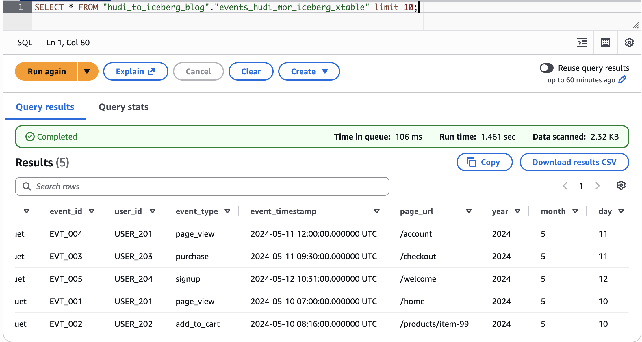
Figure 2: Validating the Apache XTable conversion by querying the migrated Iceberg table in Amazon Athena
Note: If you keep ingesting into the source Hudi table and want to keep the Iceberg table in sync, re-run the same conversion command. XTable automatically detects the previous execution and runs in incremental mode.
Migrate CoW to Iceberg
For the CoW table, update the datasetConfig.yaml with the CoW table path and name.
The glueDataCatalog.yaml, conversion command, and verification steps remain the same as described in the MOR example.
Migrate Hudi tables to Iceberg with full table migration
Full table migration (also called shadow migration) reads all data from Hudi and writes it into a brand-new Iceberg table. This approach:
Allows schema and partition evolution (for example, switching to Iceberg hidden partitioning).
Produces a clean Iceberg table with no Hudi metadata dependencies.
Requires additional storage (data is copied)
Two options are demonstrated:
Option A: CTAS – a single-statement CREATE TABLE ... AS SELECT.
Option B: CREATE + INSERT – explicit table creation followed by data insertion.
Note: When performing a full table migration, the process is the same regardless of whether your source is a Hudi CoW or MoR table. This is because Spark reads from the Hudi real-time view by default, which reflects the latest table state. For CoW tables, this means reading the current base Parquet files. For MoR tables, the real-time view automatically merges the base Parquet files with any pending delta log files, ensuring all recent inserts, updates, and deletes are captured. As a result, the migrated Iceberg table will contain a complete and up-to-date snapshot of your data, with no additional compaction or cleanup steps required before migration.
We have taken a Hudi CoW table example to demonstrate the migration from Hudi CoW table to Iceberg table.
Prepare the column list for migration
Filter out Hudi internal metadata columns (_hoodie_*) and explicit partition columns to use Iceberg hidden partitioning.
Code:
# Build column list excluding Hudi metadata and explicit partition columns
all_columns_cow = spark.sql(f"SELECT * FROM {db_name}.{hudi_events_cow_table} LIMIT 1").columns
non_hoodie_columns_cow = [col for col in all_columns_cow if not col.startswith("_hoodie")]
partition_cols = ['year', 'month', 'day']
data_columns_cow = [col for col in non_hoodie_columns_cow if col not in partition_cols]
columns_to_select_cow = ", ".join(data_columns_cow)
print(f"Columns for COW migration: {columns_to_select_cow}")
Output:
Columns for COW migration: event_id, user_id, event_type, event_timestamp, page_url
Migrate CoW to Iceberg (full table / shadow migration)
We show two full-migration options: a single-statement CTAS and an explicit CREATE followed by INSERT.
Option A: CTAS (CREATE TABLE AS SELECT)
Single statement that creates the Iceberg table and populates it in one step. Here we also adopt Iceberg hidden partitioning by days(event_timestamp) – no need for explicit year/month/day columns.
Code:
spark.sql(f"""
CREATE TABLE glue_iceberg.{db_name}.{iceberg_cow_full_ctas}
USING ICEBERG
PARTITIONED BY (days(event_timestamp))
LOCATION 's3://{bucket_name}/{db_name}/{iceberg_cow_full_ctas}/'
AS (SELECT {columns_to_select_cow} FROM {db_name}.{hudi_events_cow_table})
""")
Code:
# Verify CTAS migration
print("Iceberg COW (CTAS) - Full Migration")
spark.sql(f"SELECT * FROM glue_iceberg.{db_name}.{iceberg_cow_full_ctas} ORDER BY event_id").show(truncate=False)
Useful when you need more control over the target table schema or want to add table properties before loading data, such as sort order. It is also a good fit for very large source tables, because the load phase is a plain INSERT INTO that you can run partition by partition, giving you control over parallelism, resource usage, and resumability during the migration.
spark.sql(f"""
INSERT INTO glue_iceberg.{db_name}.{iceberg_cow_full_create_insert}
SELECT {columns_to_select_cow}
FROM {db_name}.{hudi_events_cow_table}
""")
Code:
# Verify CREATE + INSERT migration
print("Iceberg COW (CREATE+INSERT) - Full Migration")
spark.sql(f"SELECT * FROM glue_iceberg.{db_name}.{iceberg_cow_full_create_insert} ORDER BY event_id").show(truncate=False)
To avoid incurring future charges and to clean up unused roles and policies, delete the resources you created.
Clean up the S3 Tables tables and namespace (same Spark session configuration as for the S3 Tables section):
spark.sql(f"DROP TABLE IF EXISTS s3tablesbucket.{namespace_name}.{s3tables_cow_full} PURGE")
spark.sql(f"DROP NAMESPACE IF EXISTS s3tablesbucket.{namespace_name}")
Clean up the tables and namespace created in the general S3 bucket (same Spark session configuration as for the S3 General buckets section):
in_place_iceberg = [
    iceberg_cow_inplace,
    iceberg_mor_inplace,
    iceberg_cow_xtable,
    iceberg_mor_xtable,
]
for t in in_place_iceberg:
    spark.sql(f"DROP TABLE IF EXISTS glue_iceberg.{db_name}.{t}")

owned_iceberg = [
    iceberg_cow_full_ctas,
    iceberg_cow_full_create_insert,
    iceberg_mor_full_ctas,
    iceberg_mor_full_create_insert,
]
for t in owned_iceberg:
    spark.sql(f"DROP TABLE IF EXISTS glue_iceberg.{db_name}.{t}")

# --- Hudi tables ---
hudi_tables = [
    hudi_events_cow_table,
    hudi_events_mor_table,
]
for t in hudi_tables:
    spark.sql(f"DROP TABLE IF EXISTS {db_name}.{t}")

spark.sql(f"DROP DATABASE IF EXISTS {db_name} CASCADE")
On the Amazon S3 console, navigate to the database folder and delete it.
In the AWS Glue console, under ETL jobs, select the created notebook and choose Actions, Delete job(s).
In the IAM console, delete the role you created for the notebook.
Conclusion
This post outlined strategies for migrating Apache Hudi tables to Apache Iceberg on Amazon S3 and Amazon S3 Tables, enabling organizations to build a modern transactional data lake. Most of the migrations were performed from AWS Glue 5.1 notebooks with interactive sessions, with the exception of the Apache XTable path, which was executed as a standalone Java process from a local workstation to show that cross-format conversion doesn’t require a managed Spark environment and can run anywhere a JVM is available.
The migration process, whether through an in-place migration, a full table migration, or a combination of both, should be chosen based on a thorough analysis of the data architecture and the integration pipelines that read from and write to the table. Factors to weigh include performance requirements, cost, data freshness needs, and the acceptable downtime window during the cutover. The migration should follow well-defined phases that identify the data integration patterns and use cases in play, so the selected strategy aligns with the specific requirements of each table.
Note: Always run the migration end to end in a non-production environment first and validate the migrated Iceberg table against the source Hudi table before cutting production workloads over. We recommend preparing a validation runbook with queries that compare row counts per partition, aggregate values on key metrics, latest-record checks against the preCombine field, and sample point lookups on primary keys, and running it both immediately after the migration and again after each downstream pipeline is repointed at the Iceberg table. Keep the source Hudi table available until the validation runbook has passed on production traffic.
NVIDIA’s CEO and Co-Founder Jensen Huang has resigned from the company, effective immediately, marking a pivotal moment for the company and the AI and graphics industries at large
The
International Organization for Standardization (ISO) has blessed seven C++
language revisions since 1998.
The language is mostly developed by ISO’s
Working Group 21, which
considers proposed additions and amendments, integrates them into a document,
and then presents that document to the main ISO body to be voted on as a
standard. On October 23, for the first time ever, ISO declined to ratify a document
presented by Working Group 21, leaving the future of the C++26 standard in
doubt. The decision was driven by controversy around a proposed new “contracts”
feature that would add pre- and post-conditions to function signatures.
Daniel Stenberg reflects
on the 30th anniversary of the curl project.
libcurl runs in an estimated thirty billion installations today. It
is a rough estimate since the majority of all libcurl users never
tell us they use it, but we need to find it mentioned in their
credit screens, open source license windows or their manuals. A
super popular app might use libcurl today and not tomorrow, or vice
versa, which can make the numbers shift by several billions
overnight. In reality of course, once the pulse raise has calmed
down and your ego is content, these numbers do not matter. In our
corner of the world, things don’t change notably when we go from a
thousand installs to billions. We still work with similar people,
in similar ways, with similar challenges.
Penlink’s Webloc is an application that locates people using information from the weather, gaming, email, and religious apps on their phone. It’s sold to the police.
The tool collects vast quantities of location data from smartphones via commonly used weather, gaming, email and religious apps. It can build a detailed picture of where a smartphone has been over the past 12 months, and update the data hourly, showing the movements of people on a near real-time basis. Law enforcement officers can use Webloc to zero in on a map and look at all phones that were present at a specific place and time, analyzing “billions of location data points,” according to company documents reviewed by Bloomberg.
There’s a nice infographic that explains how the system works at the link.
На 10 ноември 1989 г. падна Тодор Живков. С него обаче не изчезнаха хората, контактите, информацията и зависимостите, натрупани от репресивния апарат на комунистическия режим. Промяната на политическата система се…
Не съм отворена спрямо сексуалната си ориентация, защото тази тема никога не е била засягана в училище преди и след закона. „Пропаганда“ никога не е имало.
Думите са на анонимна 12-класничка от София, взела участие в третото национално проучване (след първото от 2018 г. и второто от 2024 г.) на нагласите към ЛГБТИ+ учениците в българските училища. То е проведено през лятото на 2026 г. от Фондация „Сингъл Степ“, а в доклада върху изследването с правен анализ се включва и Сдружение „ЛГБТИ Действие“. Следва да отбележа, че бях редакторка на доклада, както и на този от 2024 г.
Актьори четат цитати от участници в изследването на „Сингъл Степ“
Анализът на резултатите включва отговорите на 1071 ЛГБТИ+ младежи от всички 28 области в България.
Респондентите са между 14- и 20-годишни и през учебната 2025/2026 г. са били ученици. Проучването, както и подборът на участниците са осъществени изцяло онлайн. То не е представително, но няма и как да бъде. Както уточних и в статията си за втората вълна на изследването от 2024 г., не е възможно да има представително изследване на ЛГБТИ+ хората. Защото не знаем колко са те и какви са основните им социално-демографски характеристики.
Въпреки това обаче методологията на проучването е изключително прецизна и е скрупульозно описана в доклада. Тя е изработена по образец на методологията на Националното проучване на училищния климат на американската организация Glisten.
пропаганда, популяризиране или подстрекаване по какъвто и да е начин, пряко или косвено, на идеи и възгледи, свързани с нетрадиционна сексуална ориентация и/или определяне на полова идентичност, различна от биологичната.
Проучването си поставя за цел да се разбере дали за ЛГБТИ+ учениците са настъпили промени след приемането на т.нар. закон за ЛГБТ пропагандата и ако да – какви са те. Това се установява по два начина. Първо, във въпросника е включен специален панел за последствията от закона. Второ, наличието на три вълни от изследването дава възможност за проследяване на тенденции – как се променят отговорите на едни и същи въпроси, зададени през 2018, 2024 г. и след закона – през 2026 г.
Последствията от закона
В края на май 2026 г. депутати от „Да, България“ внесоха в Народното събрание предложения за промени в ЗПУО, между които беше и отпадането на забраната на т.нар. ЛГБТ пропаганда. След последвалата вълна от хомофобски реакции обаче оттеглиха предложението за отпадане на забраната. Елисавета Белобрадова, която беше една от вносителките, защити оттеглянето с аргумента, че тази тема е изместила общественото внимание от останалите предложения на „Да, България“, и заяви (оригиналният правопис в този и останалите цитати е коригиран):
Интересът на обществото бе привлечен към едно-единствено предложение за отпадане на един „мъртъв“ текст, касаещ измислен и несъществуващ проблем, за който няма и никога не е имало нито един регистриран сигнал в МОН. Няма и да има.
Да, проблемът с „ЛГБТ пропагандата“ в училище е „измислен и несъществуващ“. Може ли обаче да настъпят реални вреди, ако забраните нещо, което не съществува?
Резултатите от изследването на „Сингъл Степ“ показват, че отговорът на този въпрос е положителен. Близо 80% от респондентите посочват, че знаят за закона – доста висока степен на осведоменост, като се има предвид, че тийнейджърите по принцип не се интересуват особено от законодателни промени. От тях близо една четвърт (23,8%) са чули учител или друг член на училищния персонал да се оправдава със закона, като прави негативни коментари за ЛГБТИ+ хората. Повече от половината (52,1%) имат съученици, които са постъпвали по същия начин. 29% пък са чули от работещи в училището, че заради закона или заради официална политика не може да се обсъждат ЛГБТИ+ теми в положителен контекст.
23,8%
са чули учител или друг служител да се оправдава със закона и да прави негативни коментари за ЛГБТИ+ хората
52,1%
имат съученици, които са постъпвали по същия начин
29%
са чули от работещи в училището, че заради закона не може да се говори положително за ЛГБТИ+ теми
Данни: Фондация „Сингъл Степ“, проучване 2026 г.
Понякога цензурата се отразява и на теми, включени в учебната програма – респондентка осмокласничка например споделя:
Тази година изучавахме Сафо по литература и госпожата предварително ни предупреди да не споменаваме нищо, свързано с лесбийство, че иначе ще трябвало да си учим произведението вкъщи сами.
Заради закона са настъпили промени и в достъпа до информация на респондентите. Поне на онези респонденти, в чиито училища е имало информация по ЛГБТИ+ теми – от 87-те участници, отговорили свободно на въпроса дали изобщо е имало подобни ресурси в училище преди закона, 79 отговарят отрицателно. А 106 от знаещите за закона (14,8%) познават поне един ЛГБТИ+ ученик, който по някакъв начин е бил репресиран от училищния персонал – наказан, докладван, разкрит или набелязан.
Затова не е изненадващо, че близо 80% смятат, че законът ги кара да се чувстват по-невидими, а според 46,4% след въвеждането му положението на ЛГБТИ+ учениците в училището им се е влошило. Според почти толкова (43,1%) пък положението си е същото като преди. Но ако климатът и преди не е бил подкрепящ, „същото“ означава „пак лошо“. Респондент 12-класник обобщава ситуацията със следните думи:
Мога да кажа, че учители, които си бяха хомофобски настроени преди закона, все още говорят негативно за ЛГБТИ общността в часовете. Някои учители, които имат донякъде положително отношение към ЛГБТИ общността, вече не говорят за ЛГБТИ теми, само един учител тази година заяви пред класа, че подкрепя ЛГБТИ обществото.
Не е учудващо и че почти половината от запознатите със закона не смеят да повдигат ЛГБТИ+ теми в час. Според 38,1% законът е влошил психичното им здраве, а малко над половината не смеят да потърсят подкрепа в училище заради притеснение от закона или от училищните политики. А понякога търсенето на подкрепа допълнително би влошило нещата. Един от респондентите например споделя:
Психоложката е била казала на нашите: „Ама нали знаете, че сега с този закон […] ние не можем да говорим за толерантност.“
47,6%
са по-малко склонни да повдигат ЛГБТИ+ теми в час
38,1%
оценяват, че законът е влошил психичното им здраве
51,9%
са избягвали да потърсят подкрепа в училище заради закона или училищните политики
Данни: Фондация „Сингъл Степ“, проучване 2026 г.
От друга страна, законът може да се използва и за разправа с учители, които не се харесват на някои от учениците си:
Миналата година целият ми клас беше направил план за уволнение на госпожата ни […]. Питаха я дали подкрепя ЛГБТ, тя отговори, че подкрепя хетеросексуалните, понеже нейните деца са били хетеросексуални, но пък би ги подкрепяла, ако са били и хомосексуални. След това класът ми отиде при класната и съобщи, че госпожата е била говорила за гейовете […] Госпожата просто беше строга и не я харесваха, но пък подобно [нещо би] могло да се случи на реален учител, който е гей, транс, т.н. Този закон е опасен.
Тревожни тенденции
Тенденциите, които анализът на изследването проследява, са групирани в пет области. Първата включва теми, свързани с тормоза и безопасността в училище. Втората изследва какви са ресурсите за подкрепа, до които участниците в трите вълни на изследването имат достъп в училище и вкъщи. Третата е посветена на психичното здраве и включва болезнени теми, като например отношението към самоубийството. Четвъртата е посветена на нагласите към емиграция на респондентите, а петата – на сигнализирането за случаи на тормоз и нападение.
Но вместо да преразказвам доклада, нека спомена някои от най-притеснителните тенденции, при които през 2026 г. се наблюдава статистически значима разлика спрямо 2024 г. и 2018 г. Започвам с най-тревожния резултат:
През 2026 г. повече от половината респонденти – 58,5%, сериозно са обмисляли опит за самоубийство през последните 12 месеца.
За сравнение, през 2024 г. подобни суицидни идеи са имали 49,4% от отговорилите на този въпрос. Ръстът спрямо 2024 г. е 9,1 процентни пункта. Ако делът на участниците, които поне веднъж са били нарочно изключвани или изолирани от съучениците си, през 2018 г. и 2024 г. е 71,1%, през 2026 г. той вече е 80,7%. Онлайн тормоз или заплахи поне веднъж са преживели 40,8% от респондентите през 2026 г. Точно една трета от участниците избягват тоалетните, понеже ги е страх. През 2024 г. така са постъпвали една четвърт, а през 2018 г. – една пета.
Сериозно са обмисляли опит за самоубийство
42,1%
2018 г.
49,4%
2024 г.
58,5%
2026 г.
Изключвани или изолирани от съученици
2018 г.71,1%
2024 г.71,1%
2026 г.80,7%
Преживели онлайн тормоз или заплахи
2018 г.34,1%
2024 г.35,5%
2026 г.40,8%
Избягват тоалетните заради несигурност
2018 г.20,3%
2024 г.24,8%
2026 г.33,3%
Данни: Фондация „Сингъл Степ“, проучване 2026 г.
Нараства и делът на участниците, според които съучениците им не приемат ЛГБТИ+ хората – от 54% през 2018 г., през 57,6% през 2024 г., до 63% през 2026 г. Същото се отнася и до хомофобските подмятания – от 40% през 2018 г. до 54,2% през 2026 г. Една от респондентките споделя:
В училище винаги чувам някой да нарича друг „гей“ или „лесбийка“ по негативен начин. Няколко пъти са ме питали дали съм лесбийка, и винаги трябва да кажа „не“, но усещам колко ми трепери гласът и как изчаквам малко, преди да отговоря, и как сърцето ми започва да тупти по-бързо. Когато чуя съученик да говори лошо за ЛГБТ, винаги искам да питам защо мисли така, но просто замълчавам от страх.
Съучениците не приемат ЛГБТИ+ хората
2018 г.54%
2024 г.57,6%
2026 г.63%
Повечето ученици правят хомофобски подмятания
2018 г.40%
2024 г.48,3%
2026 г.54,2%
Данни: Фондация „Сингъл Степ“, проучване 2026 г.
След приемането на закона се затвърждават и половите стереотипи. Например все повече респонденти чуват често или много често упреци към момичета, че не изглеждат достатъчно „женствени“ – 46,6% спрямо около 36% за предишните две издания на изследването. При аналогичния упрек към момчета – че не изглеждат достатъчно мъжествени – резултатът от 65,9% представлява статистически значимо увеличение само спрямо 2024 г., когато така са отговорили 55,3%, докато шест години по-рано нагласите към мъжествеността са подобни на днешните – 62,1%.
При това общо влошаване на климата в училище не е учудващ спадът в дела на участниците, които са разкрити за сексуалната си ориентация или половата си идентичност пред всичките си съученици. Докато през 2018 г. са разкрити 12,1%, през 2024 г. малко повече – 12,3%, две години след приемането на закона се наблюдава срив до 6,8%. Не е изненада и че чувството за принадлежност към училището прогресивно отслабва, както се вижда на графиката по-долу.
Подмятания за момичета, че не изглеждат достатъчно „женствени“
2018 г.36,1%
2024 г.36%
2026 г.46,4%
Подмятания за момчета, че не изглеждат достатъчно „мъжествени“
2018 г.64,1%
2024 г.55,3%
2026 г.65,9%
Разкрити пред всички съученици
2018 г.12,1%
2024 г.12,3%
2026 г.6,8%
Не чувстват, че принадлежат към училището си
2018 г.52,4%
2024 г.59,6%
2026 г.67,4%
Данни: Фондация „Сингъл Степ“, проучване 2026 г.
Що се отнася до чувството за принадлежност към училището,
следва да споменем, че някои от въпросите, зададени в изследването, съвпадат с въпроси, на които са отговаряли учениците (15–16-годишни) в международното представително изследване PISA през 2025 г. В доклада се отделят отговорите на участниците в проучването на „Сингъл Степ“, които са на същата възраст, и се сравняват с дадените от българските ученици за PISA.
Резултатите от съпоставката показват, че ЛГБТИ+ респондентите в тази възрастова група се чувстват много по-отчуждени от училището спрямо връстниците си в България. Например според резултатите от PISA над 80% от 15–16-годишните ученици в България лесно създават приятелства в училище, докато през 2026 г. по-малко от половината от връстниците им в изследването на „Сингъл Степ“ отговарят така.
Пълноценна част от училището се чувстват 76,3% от всички спрямо близо два пъти по-малко – 39%, от ЛГБТИ+ ученици. Три четвърти от всички спрямо малко над 44% от респондентите на „Сингъл Степ“ се чувстват харесвани в училище, а близо 24% спрямо 61,8% се смятат за аутсайдери. Подобни са отговорите и на въпроса дали учениците се чувстват странно и не на място в училище. Самота изпитват 1/5 от 15–16-годишните спрямо близо половината от ЛГБТИ+ връстниците им сред респондентите на „Сингъл Степ“. Както казва една участничка в изследването:
Понякога се чувствам, като че ли никога няма да съм като връстниците си, и това е факт […] и съм по-склонна да стоя в тишина и да потъвам в собствените си мисли, отколкото да разговарям с класа ми.
Ученици на 15–16 години
Лесно създават приятелства
PISA 2025 г.82,6%
ЛГБТИ+ 2026 г.48,3%
Чувстват се пълноценна част от училището
PISA 2025 г.76,3%
ЛГБТИ+ 2026 г.39%
Мислят, че съучениците ги харесват
PISA 2025 г.75%
ЛГБТИ+ 2026 г.44,3%
Чувстват се аутсайдери
PISA 2025 г.23,9%
ЛГБТИ+ 2026 г.61,8%
Чувстват се странно и не на място в училище
PISA 2025 г.26,2%
ЛГБТИ+ 2026 г.61%
Чувстват се самотни в училище
PISA 2025 г.20,5%
ЛГБТИ+ 2026 г.47,7%
Данни: PISA 2025 г. и „Сингъл Степ“ 2026 г.
Отчуждението не е само от училището, а и от държавата.
И през трите вълни на изследването над 80% (за 2026 г. делът е 88,25) планират или обмислят да напуснат България. От тях през 2026 г. 77,8% посочват идентичността си като част от причините да емигрират (две години по-рано този дял е 72,3%, а през 2018 г. – 51,9%). А 72,2% от учениците, които знаят за закона за „ЛГБТ пропагандата“, биха напуснали страната заради него.
88,25%
планират или обмислят да напуснат България
От тях – посочват идентичността си като част от причините да емигрират
2018 г.51,9%
2024 г.72,3%
2026 г.77,8%
72,2%
от учениците, които знаят за закона за „ЛГБТ пропагандата“, биха напуснали страната заради него
Данни: Фондация „Сингъл Степ“, проучване 2026 г.
Ето какво казват за емиграцията някои от участниците в изследването:
Хората и преди този закон бяха много токсично настроени към ЛГБТИ+ хората. Хомофобията е страшно нещо, особено в България. Често съм мислила, че е време да се местя. Тук няма да бъда приета.
Единственото нещо, което законът постигна, е да покаже, че младежите от тази прослойка нямат бъдеще в България.
Приетият закон позволява аз и хората като мен да бъдем тормозени и да си мислим за бъдеще в чужбина, където това, което сме, няма да бъде считано за „неморално“ и странно.
Стадии на отчуждението
Резултатите от трите издания на проучването на „Сингъл Степ“ разкриват плашеща картина след промените в ЗПУО. Средата в училище, където ЛГБТИ+ младежите прекарват голяма част от времето си, е станала по-неприемаща и враждебна. Дискриминационната реторика на политическо равнище се отразява негативно и на отношенията у дома – ако през 2024 г. 40,9% от респондентите не са били разкрити пред нито един член на семейството си, през 2026 г. така постъпват вече близо половината – 49,9%. Това обяснява защо участниците в изследването са все по-отчуждени.
Отчуждението обаче има степени. Първо ЛГБТИ+ младежите не се чувстват на мястото си в училище и/или вкъщи. В резултат на дискриминационното законодателство и враждебния климат в обществото обаче голяма част от тях не виждат бъдещето си в България, а искат да емигрират.
Ала най-радикалната форма на отчуждение е отказът от живота.
Фактът, че през 2026 г. близо 60% от ЛГБТИ+ младежите, участвали в проучването на „Сингъл Степ“, сериозно са обмисляли самоубийство, би трябвало да бъде червена лампа за институциите. Защото най-високата цена, която плащаме за популисткото и насаждащо омраза законодателство, е човешкият живот.
Помните ли, когато кината бяха много, а филмите – малко и пристигаха през гъста идеологическа цедка с по година-две закъснение? Подвиквали ли сте умолително „Повече билети?“ пред вратите на разпродадена зала преди прожекцията? Още ли ви боли от закриването на любимите ви салони, или по-лошо – обръщането им на магазини и хотели? Ако да, то вероятно сте отдавнашни участници в съдбата на „Световната кинопанорама“, която в зората на демокрацията се превърна в „Киномания“ и устоя четири десетилетия въпреки недалновидните или направо несъществуващи български културни политики, конкуренцията на стрийминг платформите и варварското нашествие на телефоните срещу големия екран.
Ако пък сте от по-скорошните попълнения в киноманската публика, то сега е моментът да видите какво и как е било. На 12 ноември късометражният филм на Борис Мисирков и Георги Богданов „Киномания: началото“ще ни даде тази възможност, преди юбилейното издание на фестивала да започне официално с „Див кон девет“ на Мартин Макдона – превъзходна трагикомедия, която уж е разположена в далечни ширини и времена, но прокарва смразяващи паралели с настоящето.
София Лорен и Марчело Мастрояни в „Един особен ден“ (1977) / Кадър от „Слънце, лято и студенти“ (1922), реж. Лау Лаурицен-баща
Сами по себе си
Повечето филми от „Киномания 2026“ имат поне по 3–4 прожекции, та си струва да започнем с няколко събития, които са само по веднъж, а не бива да се пропускат.
Преди сто години зрителите в русенското кино „Олимпия“ присъстват на паметна прожекция концерт: датска романтична комедия, придружена от джаз на живо. На 28 ноември т.г. от 20:00 ч. в „Люмиер“ триото „Братя Владигерови“ ще съпроводи с музика на живо същия ням филм – „Слънце, лято и студенти“, един от десетките с прочутата някога хумористична двойка Крачун и Малчо – и по всичко изглежда, че също ще е славно.
Пак за 28 ноември, но от 16:00 ч., в „Одеон“ е предвиден шедьовърът на Ѐторе Скола„Един особен ден“. Свещените чудовища на италианското кино София Ло̀рен и Марчело Мастрояни нерядко са играли заедно, но никога така впечатляващо, както тук. Денят от заглавието е онзи, в който през 1938 г. Хитлер приключва гостуването си на Мусолини в Италия. Докато по майските улици фашистите скандират с плам в чест на нацистите, в притихнала римска кооперация се разиграва странната, отчаяна среща сблъсък на една презряна от семейството си многодетна домакиня и един презрян от режима интелектуалец…
Агата Туркот в щастливото начало на „Дом добър“ на Смажовски
„Кинотека“ е заглавието на полския раздел в рамките на фестивала: всяка от седемте творби в него ще се прожектира еднократно и безплатно от 19:00 ч. в Дома на киното. Три филма – „Обетована земя“, „Катин“ и „Остатъчни образи“ – представят различни епохи от творчеството на Анджей Вайда, стогодишнината от чието рождение отбелязахме на 6 март. Но може би най-належащ за гледане в подборката (на 15 ноември) е Dom dobry на Войчех Смажовски – друг полски великан, чиито съвременници имаме късмета да сме.
Смажовски често работи с едни и същи актьори и не страни от най-болезнените теми –
създава сложни истории, способни да те превземат отвътре и да те държат с месеци.
Може да се каже, че „Дом добър“ (лош превод и непрехвърлен мост към друг важен филм на автора, Dom zly, познат у нас като „Къщата на злото“) е за домашното насилие, само че така фината му, многослойна тъкан ще бъде несправедливо банализирана. Интелигентна млада жена попада в минираната територия на гаслайтинга и съзнанието ѝ влиза в драматичен конфликт с изопачената от други реалност. В един момент героинята е толкова объркана, че смисълът на вече преживяното и посоката на предстоящото в главата ѝ започват конвулсивно да се променят – Dom dobry възхитително и плашещо изобразява тъкмо това.
Наричат Смажовски „екзорсист на националните демони“, но демоните тук са от най-интернационалните.
За „Страхливец“ дебютантът Еманюел Макия спечели в Кан награда за най-добър актьор / Матилде Арсел в ролята на изстрадалата Мари в „Непозната жена“
Някои от най-обсъжданите
филми с премиера през изтеклата година са – както винаги – в сърцевината на фестивалната програма. И ако от тях трябва да откроя по-специално един, то той ще е „Страхливец“ на Люкас Донт – заради майсторството на екипа и поетичната му мощ, която от калния ад на Първата световна война успява по оригинален начин да извлече нещо сладостно за споделяне. Хуманността, изкуството и свободата като противоотрова срещу цинизма и страха са ни остро необходими сега и винаги.
Апропо за „Страхливец“ вече говорихме в репортаж от Карлови Вари, в който с добро споменахме и „Любимо същество“ на Родриго Сорогойен – и той селектиран за „Киномания 2026“, но под заглавието „Обич“(гледайте го, Хавиер Бардем и Вики Луенго правят чудни роли).
От Берлин със „Златна мечка“, от Кан със „Златна палма“ и от Венеция със „Златен лъв“ в София, Пловдив, Стара Загора идват отличниците на 2026-та: „Жълти писма“ на Илкер Чатак (Турция), „Фиорд“ на Кристиян Мунджиу и „Непозната жена“ на Май ел-Туки (Дания). Знаменателно е, че и трите обрисуват травмиращия натиск върху индивида от страна на колективната машина, поела в грешна посока.
В „Жълти писма“авторитарната държава санкционира артисти за възгледите им. Във „Фиорд“ едно семейство е убедено, че институциите го насилват, докато институциите са убедени, че се борят с насилието в семейството. В „Непозната жена“отшумяващата Втора световна война вдига тежка мътилка и „добрите“ със смущаваща лекота стават „лоши“… „Непозната жена“ би бил моят избор от трите, ако избор се налагаше – освен поглед към една размирна епоха той е и точен обзор на част от начините, по които жената е била (и в много места и случаи си остава) една неизвестна и недогледана от обществото величина, често третирана като предмет.
Неотдавна в репортаж от Сан Себастиан обсъдихме по-пространно „Фиорд“, като пътьом зачекнахме безрадостната сивота на „Минотавър“на Андрей Звягинцев и смисленото усилие на „Джоузефин“/„Жозефин“ на Бет де Араужо, а в друг текст от същия фестивал се порадвахме на милата северна история „Ледена земя“ на Аманда Кернел и се разочаровахме от предвидимия „Дебютът“ на Джеси Айзенбърг. Всички те са на „Киномания 2026“, както и „Черни пари за бели нощи“на Кристина Грозева и Петър Вълчанов, за който казахме няколко сдържани думи от Карлови Вари. Хубаво е, че в идните дни ще можем да ги гледаме и в България и да поспорим.
Автопортрет на документалиста Марк Казънс
Един от най-коментираните филми в момента е „Можеш да видиш всичко“на Ланс Опенхайм и Нейтън Фийлдър. В него е направен опит за доближаване до Елизабет Холмс, основателката на компанията „Теранос“, която уж изобретява машинка за бърз анализ на кръвни проби. Защо подобна машинка не съществува и е сигурно, че Холмс е наясно, че лъже, докато взема милиони от инвеститори, може да се прочете в едно кратко и ясно становище на американското Министерство на правосъдието (и в хиляди статии по цял свят).
Двамата кинаджии обаче решават да поживеят с Елизабет, капризния ѝ мъж и двете им невръстни дечица
в месеца, преди тя да влезе в затвора. В трите мъчителни часа, произтекли от това съжителство, изобилстват мълчанията, неловките обмени на фрази и свръхблизките планове, пълни с драматична музика и втренчени погледи, но не и информация или наслада. За да си съставите представа, без да си хабите живота, стига да си пуснете тийзъра и веднага след него – една или друга пародия от стотиците, наводнили YouTube.
За радост, документалистиката е представена в програмата и с нещо далеч по-съдържателно: два епизода (за 60-те и за 80-те години) от 16-часовия сериал „История на документалния филм“. Неговият автор – ирландецът Марк Казънс, ще дойде лично в „Одеон“ (на 25 ноември) и в „Люмиер“ (26 ноември), за да ги представи и да разговаря с публиката, а това наистина си заслужава: Казънс знае много, умее да намира връзки между даденостите и страстно вярва в заниманията си.
(Добра идея е да се запознаем и с другите му изследвания – 15-те епизода на „История на киното: една одисея“ например или 14-те на „Жените правят кино“, който впрочем започва с „А бяхме млади“ на Бинка Желязкова…)
„Всички обичат Бил Евънс“, реж. Грант Джи („Сребърна мечка“ за режисура) / „Татко след полунощ“, реж. Джонатан Фърстман
Упования
Възлагам специални надежди на няколко заглавия от „Киномания 2026“, които още не съм гледала. Да речем, „Големите майстори на киното“ на Паоло Чивати – защото беседите с девет съвременни режисьори, сред които Джейн Кемпиън, Асгар Фархади, Пабло Лараин и Тим Бъртън, няма как да са скучни. „Всички обичат Бил Евънс“ – заради предчувствието за елегантност (черно-бялото, джазът) и Андерш Даниелсен Ли, който умее да изиграе блестящо всичко от чувствителен изгряващ писател до морален изрод. Или „Татко след полунощ“ на актьора, сценарист и режисьор Джонатан Фърстман – тъй като беше сред любимците на младежкото жури в Сан Себастиан, а то се слави с безкомпромисния си вкус…
И още: „Дом за нея“на Мелиса Годе (истории от едно действително място за подкрепа на жени в беда) и „Изоставен от всички“на Венсан Гаренк(по реалната трагедия на учителя Самюел Пати, убит от един глупав слух и един заблуден тийнейджър) – понеже френското социално кино има високи критерии и отдавнашни традиции. И е безкрайно интересно да се гледа как едно държащо на себе си общество се справя с най-вредния си атавизъм – нагона за насилие.
Всичко е фикция. За мен документалистиката е алтернативен начин за правене на художествено кино… Веднага щом сложиш камерата някъде, ти вече тълкуваш. Един документален филм никога не е копие на реалността, а интерпретация…
Това твърди големият Никола Филибер, а от думите му резонно може да се тръгне и по обратния път: художественото кино също е вид документалистика. Съпреживяването, едновременното замисляне или заостряне на вниманието в залата е съвсем реален факт от живота на публиката. Един фестивал е не просто преглед на личните фантазии и повествователните вещини, а и поле за най-истински събития, техен архив и залог за бъдещето ни далеч извън залите.
Amazon OpenSearch Service already offers high availability within a single AWS Region through Multi-Availability Zone (Multi-AZ) deployments. Some organizations, however, need a multi-Region architecture to meet specific business requirements. These include strict recovery point and recovery time objectives, data residency mandates, and business continuity plans for mission-critical search and AI workloads.
Until now, meeting that bar on Amazon OpenSearch Service meant building and operating your own replication with cross-cluster replication or dual writes to multiple Regions. That took months of engineering and ongoing maintenance, offered no coordinated way to switch roles between Regions, and gave no guaranteed recovery point objective (RPO).
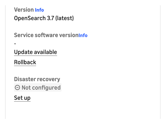
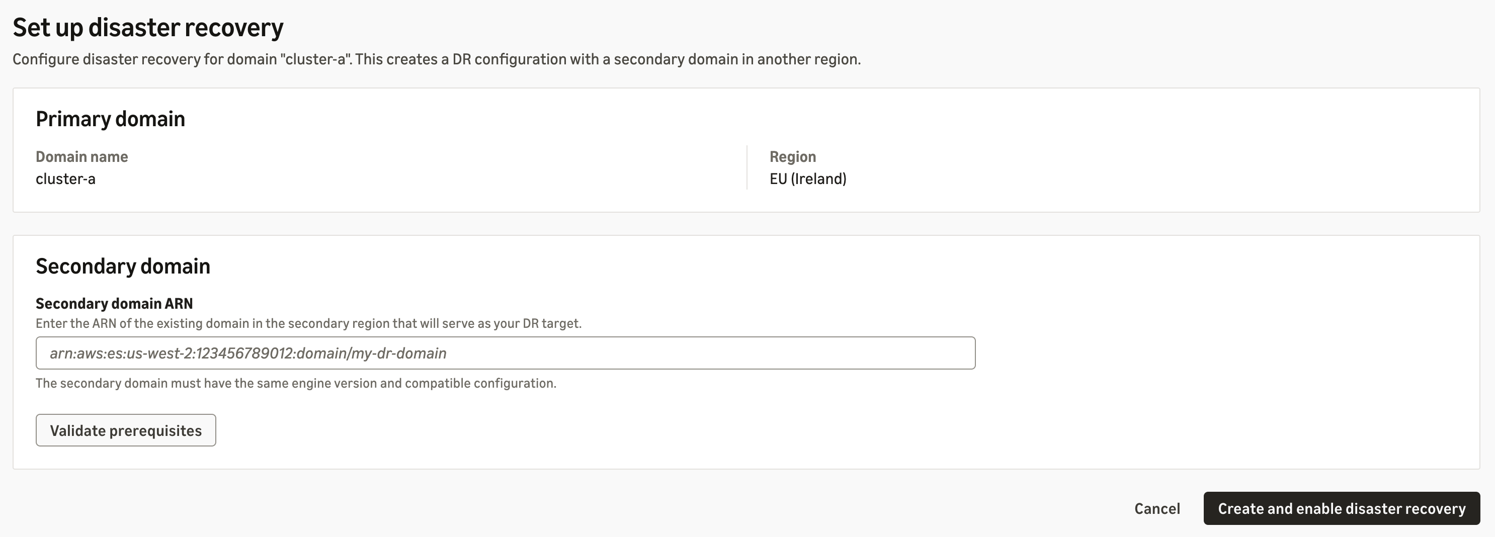
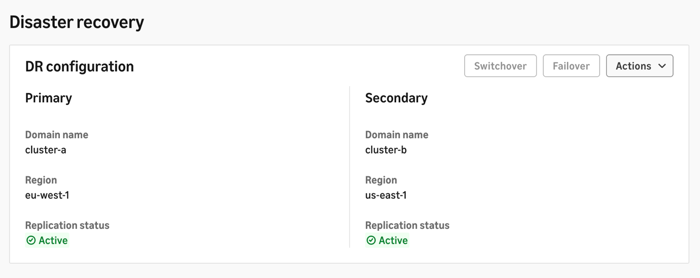
Amazon OpenSearch Service now offers managed disaster recovery for domains running OpenSearch 3.7 or later. Managed disaster recovery replicates your data from a primary domain in one Region to a secondary domain in another and keeps the secondary continuously in sync. When you need to move your workload, you use API-driven switchover and failover. It provides an RPO under 1 minute and a recovery time objective (RTO) under 20 minutes, and you can set it up in two steps.
In this post, we explain how managed disaster recovery works, what to check before you start, and how to set it up, monitor it, and switch Regions.
Who should use managed disaster recovery
Managed disaster recovery is built for workloads where downtime or data loss has a direct business, customer, or compliance cost. Common patterns include:
Customer-facing search: Ecommerce, product catalog, and site search, where downtime means lost revenue and a degraded customer experience.
Financial services and risk: Fraud detection, transaction search, and risk analytics, where regulators expect demonstrated cross-Region recoverability and regular disaster recovery exercises.
Mission-critical operational data: Search and analytics that support incident response, security investigations, or regulated record retrieval, where teams need uninterrupted access to data.
If your recovery plan requires a copy of your OpenSearch data in another Region and a tested way to move your workload there, managed disaster recovery replaces the replication pipeline you would otherwise build and operate yourself.
Solution overview
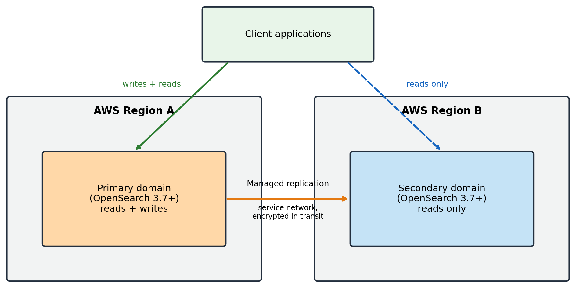
Managed disaster recovery pairs two OpenSearch Service domains in different Regions. One domain is the primary: It accepts reads and writes. The other is the secondary: It continuously receives changes from the primary and serves reads only. The following diagram shows the architecture.
Figure 1: Managed disaster recovery pairs a primary domain in one Region with a read-only secondary domain in another, with managed replication between them
When you pair the domains, the service first copies the existing Lucene segments from the primary to the secondary. After this initial copy, every new document and update is indexed on both the primary and the secondary domain. Replication traffic stays within the OpenSearch Service network, so you don’t need to set up virtual private cloud (VPC) peering or any networking, and data is encrypted in transit. Because both domains index the data, the secondary is ready to take over as primary at any time.
Both domains serve reads, but only the current primary accepts writes. When roles change, you redirect your application’s writes to the new primary. For more details, see the Switch Regions section later in this post.
There are two ways to move the primary role to the other Region. The following table compares them and later sections refer back to this table.
Switchover
Failover
Type of event
Planned
Unplanned
Coordination
Coordinated role swap between both domains.
Unilateral promotion of the secondary.
Data loss
Zero: pending writes replicate before roles swap.
Writes not yet replicated are lost, bounded by replication lag (RPO).
When to use
Regulatory exercises, maintenance, planned Region moves, issues outside OpenSearch Service.
The primary domain is unavailable.
Call on
The secondary domain being promoted.
The secondary domain being promoted.
You can also manage replication health from a built-in dashboard on the AWS Management Console, and the service supports customer managed AWS Key Management Service (AWS KMS) keys for encryption at rest.
Prerequisites and limitations
Before you start, confirm that your environment meets the following requirements:
Engine version: Both domains run OpenSearch 3.7 or later. If you’re on an earlier version, see Upgrade to OpenSearch 3.7 with a clone-based upgrade at the end of this section.
Same AWS account: The primary and secondary domains must be in the same AWS account, in different Regions.
Matching sizes: Both domains index all data and use the same number of primary shards and replicas, so they need similar CPU, memory, and storage capacity.
UltraWarm, Writable Warm, and Optimized engine for log analytics: Domains that use UltraWarm or Writable Warm storage or the OpenSearch Optimized engine for log analytics aren’t supported in this release.
Configuration isn’t replicated: Managed disaster recovery replicates data. Index State Management (ISM) policies, index templates, settings, and roles aren’t replicated, so manage them on both domains with infrastructure as code (see Best practices later in this post).
Client redirection: The service doesn’t redirect application writes after a switchover or failover. Your application or runbook must do this.
Upgrade to OpenSearch 3.7 with a clone-based upgrade
If your domains run an earlier version, you can upgrade them to OpenSearch 3.7 with a clone-based upgrade. Instead of upgrading your existing cluster in place, OpenSearch Service creates a clone of your domain on the target version and keeps it in sync with your data. Your domain keeps serving traffic from the original cluster. With a clone-based upgrade, you can:
Validate first: Test the clone with your own read requests before it takes effect.
Cut over when you’re ready: You choose when to move traffic. Writes are blocked during cutover, which can last up to several minutes.
Cancel or roll back: Cancel any time before cutover, or roll back to the original cluster during a retention period that you set.
Clone-based upgrades are available for domains running Elasticsearch 7.10 or OpenSearch 1.1 or later. Earlier versions need an in-place upgrade first. You’re charged for both the original cluster and the clone while you validate and during the retention period. Before you upgrade, take a manual snapshot and run the pre-upgrade check. For details, see Upgrading Amazon OpenSearch Service domains.
Set up managed disaster recovery
You can set up managed disaster recovery on the console or with the AWS Command Line Interface (AWS CLI). In both cases, the flow is:
Create the primary domain (OpenSearch 3.7 or later) and start indexing and searching.
Create the secondary domain of the same version in a different Region, with matching size.
Pair the primary with the secondary.
Check the replication status.
Set up on the console
On the AWS Management Console, open Amazon OpenSearch Service and select your primary domain. The disaster recovery section is available for domains running OpenSearch 3.7 or later.
Figure 2: The domain summary shows the disaster recovery status as Not configured with a Set up link
Figure 3: An information banner offering a Set up disaster recovery button
Choose Set up or Set up disaster recovery, and then enter the Amazon Resource Name (ARN) of the secondary domain.
Figure 4: The setup page, where you enter the secondary domain ARN and validate the prerequisites
Choose Validate prerequisites. When the domains are compatible, the console displays the message “These domains can be paired for disaster recovery.” Choose Create and enable disaster recovery. Pairing takes a few minutes.
Set up with the AWS CLI
Run the following command in the primary Region to add the secondary domain as a replication peer:
Before pairing, you can call the CompareDomainConfiguration API to find where the two domains’ configurations differ across key categories.
Check the replication status
On the console, choose Manage in the disaster recovery section to view the peer role and replication status.
Figure 5: The disaster recovery dashboard, showing both domains with an Active replication status
With the AWS CLI, call DescribeDomainReplication on either domain to see the peer role and replication status. To stop replication, call RemoveReplicationPeer. Each domain keeps its data.
Use switchover for planned events and failover when the primary is unavailable (see the comparison table in Solution overview). In both cases, call the API on the secondary domain that you’re promoting.
Perform a planned switchover
SwitchoverReplication performs a coordinated role swap with zero data loss. Run it on the secondary domain:
FailoverReplication promotes the secondary to primary unilaterally. Data written to the old primary but not yet replicated is lost. The loss is bounded by the replication lag. Because of this, the command requires the --allow-data-loss flag:
Managed disaster recovery doesn’t redirect your applications. Both domains stay readable, but only the primary is writable, so after a switchover or failover your applications must send writes to the newly promoted primary. Make the write-path update part of the same runbook step as the API call, for example by updating a DNS record, a configuration parameter, or a service discovery entry.
After a switchover or failover
After a switchover, the former primary becomes the secondary and replication continues in the reverse direction with no further action.
After a failover, when the original domain is available again, you can fail back. The original domain needs to be re-seeded before it can be used again for replication. After the re-seed, you can switch over to restore the original primary Region.
Performance results
We measured setup, initial sync, steady-state replication lag, planned switchover, and unplanned failover across multiple r7g instance sizes and data footprints. The tests used synthetic Apache log data with a sustained write load of 240 MBps.
Domain details:
R7g.4xlarge domain: 6 data nodes + 3× m7g.large cluster managers, 12 TiB gp3 per node.
R7g.8xlarge domain: 6 data nodes + 3× m7g.large cluster managers, 12 TiB gp3 per node.
Indices use 12 primary shards + 1 replica, rollover at 50 GB per primary shard.
Note: Results can vary by workload, data size, and configuration.
Setup and initial sync
Pairing is one API call and completed in 1 to 3 minutes in our tests, from 1 TiB to 10 TiB. Initial sync time depends on data size.
Data
Instance
Turn on disaster recovery
Full initial sync
1 TiB
r7g.4xlarge
~1 min
20min
10 TiB
r7g.4xlarge
~1 min
2 hr 31 min
10 TiB
r7g.8xlarge
~1 min
2 hr 18 min
Steady-state replication lag
Replication lag is how far behind the secondary is under sustained write load, measured with DisasterRecoveryReplicationLagTime (p95 over the test window).
Data
Instance
Write load
Replication lag (p95)
1 TiB
r7g.4xlarge
240 MBps
~10 s
10 TiB
r7g.4xlarge
240 MBps
~10 s
10 TiB
r7g.8xlarge
240 MBps
~10 s
Planned switchover
Pending writes replicate to the new primary before the role swap completes, so data loss is zero. RTO is how long clients see writes fail before the new primary accepts them.
Data
Instance
Write load
Writes down (RTO)
Data loss
1 TiB
r7g.4xlarge
240 MBps
36.8 s
0
10 TiB
r7g.4xlarge
240 MBps
38 s
0
10 TiB
r7g.8xlarge
240 MBps
57 s
0
Unplanned failover
RPO is how many seconds of writes were lost. Role flip confirmed is how long until the control plane confirms the promotion. Writes down is how long until clients receive HTTP 201 from the new primary.
Data
Instance
Write load
Role flip confirmed
Writes down (RTO)
Data loss (RPO)
1 TiB
r7g.4xlarge
240 MBps
6.4 s
69 s
~8 s (~2.0M docs)
10 TiB
r7g.4xlarge
240 MBps
8.1 s
61 s
~10 s (~2.46M docs)
10 TiB
r7g.8xlarge
240 MBps
5.8 s
60 s
~10 s (~2.46M docs)
Key takeaways
In our tests, we saw the following results:
RPO: Unplanned failover lost about 8 to 10 seconds of writes, well within the under-1-minute RPO target. Planned switchover lost no data.
RTO: Writes resumed in about 1 minute after failover and under 1 minute after switchover, well within the under-20-minute RTO target.
Scale: Pairing time, lag, and recovery times stayed roughly constant from 1 TiB to 10 TiB. Only the one-time initial sync grows with data size.
Best practices
Manage configuration with infrastructure as code – Keep index templates, ISM policies, settings, and roles in a Git repository and apply them to both domains, for example with the OpenSearch Terraform provider.
Upgrade the secondary first – When upgrading engine versions, upgrade the secondary domain first and the active primary last. We recommend testing the performance of the new version on the secondary, then upgrading the primary after the secondary domain upgrade is validated. Don’t run mixed versions permanently.
Size domains to match – Keep instance types, counts, storage, and shard configuration aligned, and use CompareDomainConfiguration to detect drift.
Decide your failover automation – Failover is manual by design, because the right trigger differs by business. You can build event-driven automation using CloudWatch alarms and the failover and switchover APIs.
Exercise your runbook – Use switchover regularly to rehearse Region moves, including the client write redirection step.
Managed disaster recovery gives Amazon OpenSearch Service domains continuous cross-Region replication, a zero-data-loss planned switchover, and a bounded-RPO failover, without building and operating your own replication pipeline. It serves regulated industries and business-critical workloads with strict availability, recovery, and business continuity requirements.
To get started:
Create or upgrade domains to OpenSearch 3.7 or later in two Regions in the same AWS account.
Pair them on the console or with the AddReplicationPeer API.
Set CloudWatch alarms on the replication metrics, and build and rehearse your switchover and failover runbook.
Every day, Zillow sends home shoppers more than 100 million personalized email and push notifications: saved search alerts, home recommendations, property updates, seller reports, and reminders. These messages are one of Zillow’s core ways to engage home shoppers, and Zillow delivers them on time with consistent behavior across every campaign. Today, each of those notifications runs as its own short-lived workflow execution on AWS Step Functions Express Workflows.
The underlying shape of this work isn’t unique to real estate. Many systems run the same kind of workflow at high volume: take an event, enrich it from several services, apply rules, assemble an output, and send it. This post shows how Zillow built one configuration-driven orchestration system to run that pattern at scale, and what teams across many domains can reuse from it.
Historically at Zillow a separate generator service produced each of these campaigns, and each service carried its own workflow, data models, and business rules. As the number of notification campaigns grew, so did duplicated engineering work, inconsistent behavior, and operational cost. Product teams needed to launch campaigns faster, reuse shared capabilities, and run consistent experiments without system-specific work.
To meet that need, the Zillow Comms Experience team, working with AWS, built two things. The first is the Campaign Orchestrator, which is a configuration-driven orchestration layer that runs each notification as a short-lived workflow execution on Step Functions Express Workflows. The second is the Universal Content Generator (UCG), a library of reusable, schema-driven content modules that those workflows call. Together they make campaign creation faster and more consistent, and they give AI-assisted tooling a declarative format to work with.
The challenge: why the original system needed replacing
The previous content generation model slowed product delivery. Zillow’s Comms Experience supported more than 20 email and push campaigns generated by more than 10 microservices. Each microservice owned its own workflow, models, business rules, and assembly logic.
Most campaigns followed the same pattern: receive a trigger, hydrate data, apply rules, assemble content, and send the message. Each campaign service implemented that pattern separately, creating duplicate engineering work and inconsistent behavior. It also added operational overhead across releases, monitoring, logs, dashboards, and on-call support.
Each campaign was built as its own service because, when these systems were first built, scale was the main challenge. As Zillow added more products, the tradeoff changed. Similar features ended up implemented differently across campaigns, so every new capability had to be rebuilt and retested in each service. That made it hard to roll out features across products and slowed development. The push to centralize came from that cost: we needed to move faster and stay consistent across every customer experience. With one shared implementation, a feature could be built once and reused everywhere, while each campaign kept the flexibility to tailor its experience. Before evaluating workflow engines, we first had to extract shared logic into reusable modules and move campaign decisions into configuration.
The following diagram shows the original architecture, where each campaign generator carries its own copy of the workflow, data models, and business rules.
Figure 1: Original system
Competitive evaluation
We evaluated Temporal, Flowable, an in-house engine, and Step Functions Standard and Express Workflows against four criteria. Those criteria were reliability, total cost of ownership, development speed, and how well the service would scale across teams. The engine had to be managed, configuration-driven, and able to orchestrate both newer and older services. Pricing also had to fit our volume.
Temporal and Flowable would have added another infrastructure component to operate. That worked against two of our core goals: cutting the release, monitoring, and on-call overhead that the original system created, and getting pilot projects running quickly. Neither is available as a managed AWS service, so we would have had to run and scale them ourselves. Step Functions is serverless, so we had no servers or worker fleets to run, and a team could start a pilot without first setting up infrastructure. An in-house engine offered control but required custom lifecycle management, worker pools, queue integration, and monitoring. Step Functions met the core orchestration needs at roughly a quarter of the estimated build effort and a quarter of the ongoing maintenance effort. It was the clear choice for the minimum viable product (MVP).
Express mode compared with Standard mode
Our planning model assumed high-throughput, low-latency workflows. The MVP plan ramped from 14 million workflows per day to more than 100 million across all campaigns. At full scale that means several thousand executions per second at peak. Each workflow runs for only a few seconds, and a notification has to arrive while it’s still relevant. We evaluated both Step Functions execution modes, and for our use case Express Workflows were the better fit.
At least once, sufficient with idempotent modules.
Our workflows are high volume, short-lived, finish well within the five-minute Express limit, and are designed around idempotent module calls. We validated quota, latency, and operational behavior during the traffic ramp-up.
The architecture
Campaign Orchestrator is a configuration-driven workflow platform. Each message is input data combined with persisted campaign configuration. The configuration is relatively static for each workflow, while the input data stays flexible based on how the configured steps are assembled.
A shared orchestration layer reads queued campaign events, groups work where appropriate, and invokes the corresponding Step Functions Express Workflow for each campaign. Campaign metadata describes product constants, ownership, and Zillow environment features. Workflow configuration describes step topology, step-level configuration, mappings, branching, delay behavior, and send behavior.
The following JSON shows a simplified workflow input, combining the message payload with the platform, campaign, and configuration metadata that drive the workflow:
The following diagram shows the new architecture, where a single shared orchestration layer and one library of reusable modules serve every campaign. A message moves through the diagram from left to right. The ingress service queues it, and the router applies campaign controls and starts the workflow. Campaign Orchestrator runs the Step Functions steps, each step calls a UCG module, and the delivery service sends the result.
Figure 2: The new system
Router
Our campaigns need a set of controls applied before a workflow starts: queue polling, batching, idempotency checks, pause and resume behavior, replay coordination, speed control, and campaign routing decisions. Some of these controls are specific to how we order and throttle campaign sends, so they live outside Step Functions.
We centralized these controls in an in-house router service that reads from Amazon Simple Queue Service (Amazon SQS) and starts the right Step Functions workflow. Keeping them in one place gives us a single point to pause a campaign, replay a batch, or adjust send speed without changing any workflow definition.
Shared modules (UCG)
The Universal Content Generator is the modular content generation layer behind Campaign Orchestrator. Instead of each campaign owning a separate generator, UCG organizes shared capabilities into reusable modules. Before UCG, this logic was spread across more than 10 separate generators. Centralizing it in one service also smoothed its traffic. Some daily campaigns used to run for about four hours and leave their generator idle for the other 20. Now all campaigns share one fleet, so the load spreads across the day.
Modules handle capabilities such as property hydration (loading listing details such as price, photos, and address for each home in a message), hidden homes (listings a user has chosen to hide, which we filter out of notifications), common data (the subscriptions, saved homes, eligibility flags, and propensity scores every campaign loads for a recipient), recommendations, A/B testing, and content assembly. They are stateless and schema-driven.
Direct service invocation with HTTP Invoke
A key design choice was to call UCG directly through Step Functions HTTP Invoke. This fits the workload for two reasons. First, our content generation logic already ran as long-lived containerized services inside our private service environment, with network access, service discovery, and authentication established. Second, routing workflow steps to UCG added no new compute cost.
With Step Functions HTTP Invoke, we call UCG modules for data hydration, rule checks, and content assembly as they already run. Authentication runs through an Amazon EventBridge connection. Each HTTP Invoke task points to the connection with a ConnectionArn. The connection holds an API key, and UCG checks that key on every request. Amazon EventBridge keeps the key in AWS Secrets Manager and adds it to the request at call time. The workflow definition never contains the key, and neither does our application code. When the key rotates, we rotate it once in the connection and every workflow picks it up.
To avoid repeating the same HTTP Invoke settings in every workflow, we introduced component inheritance. Components are written in a slightly modified version of the Step Functions task definition we deploy through AWS CloudFormation. A base component holds the settings that many steps share, and other components extend it. The following base component, content_module_call, defines how every workflow step calls UCG services directly through HTTP Invoke: the resource, method, headers, and the ConnectionArn for the connection described earlier.
Business modules extend the shared HTTP component and supply only the module endpoint. Before deployment, our build script replaces each component with a standard Task state: it loads the component named in Extends, merges the step’s own fields on top, and writes the result into the Terraform we deploy. Workflow definitions stay focused on product intent rather than network plumbing:
Step Functions state machine definitions, JSONata expressions, and infrastructure definitions are powerful, but they are not the right interface for every campaign owner. We added a higher-level configuration layer so campaign owners can define their own workflows without having to understand Step Functions CloudFormation configuration. Each campaign config describes a workflow: which modules run, in what order, and how data moves between them. The system translates that config into the Step Functions definition and CloudFormation template that gets deployed. Campaigns don’t share one generic workflow that picks modules at runtime. Each campaign gets its own workflow, built from the same shared modules and components. As a next step, we are considering a generic workflow that assembles modules in real time from config. Each campaign would still run its own copy of that workflow, so ownership stays isolated per campaign.
Campaign owners specify the modules needed for an email template or push notification. Each module exposes input, output, and configuration schemas. Campaign owners define module outputs to satisfy the template input schema. Module inputs define what triggers need to provide.
With this structure, campaign owners onboard through a declarative process. They work with configuration instead of raw workflow code or JSONata expressions. They can also run controlled experiments and give AI tools a format they can inspect, generate, and modify with appropriate validation.
The following simplified A/B test config is adapted from a real Campaign Orchestrator config. It injects an A/B test module before email transformation and maps the experiment result into the next step without directly touching Step Functions or CloudFormation definition.
Because a campaign is declared as schema-validated configuration, the same contracts that protect human changes also apply to AI-assisted tooling. Our internal assistants already draft module selections and mappings from a product brief, and the output must pass the same schema checks, JSONata tests, and Step Functions validation before it can be deployed.
Batch mode optimization
Campaign Orchestrator supports batching, which improves overall throughput while reducing cost. Instead of launching one workflow per message, the router can group messages and invoke one workflow for the batch.
For example, processing 100 messages individually could produce 100 workflow executions and 400 HTTP requests to UCG services. With batching, the same messages can be processed in one workflow with four HTTP requests, assuming each step supports bulk input and output. That matters at our volume for two reasons. Express Workflows charge for each request and for run time. Batching cuts the number of requests, but each batch runs longer. A rule of thumb: a batch of 10 messages costs less than 10 separate runs as long as it takes no more than 10 times as long as one run. In the preceding four-step example, one message takes about 1.2 seconds, so a batch of 10 saves money if it finishes within 12 seconds. In practice, a batch runs only 10 to 20 percent longer than a single message, about 1.4 seconds instead of 12. That makes a batch of 10 about 90 percent cheaper than 10 separate runs. The batched payload stays under the 256 KiB limit, so memory is still billed at the 64 MB minimum. Fewer executions and HTTP requests also use less of the StartExecution rate, HTTP Invoke concurrency, and logging throughput we size for. That leaves headroom to send more notifications on the same quotas.
The batching model appears in the Step Functions definition and JSONata expressions. This simplified example shapes a batched payload into a bulk UCG request while preserving each tracking ID:
Batching works only if every step in the workflow can handle a batch rather than a single message. For UCG, that requirement is built into the module API. Each module’s schemas define its input, output, and config models, and the module API accepts those models as a batch keyed by tracking ID. A module that doesn’t follow that API won’t build. Our JSONata mappings and upstream and downstream service contracts already accepted bulk input internally, so adding batching didn’t require reworking them.
Batching also can’t cost us visibility into individual messages. Because each batch is keyed by tracking ID, as the preceding example shows, UCG returns a result from each module for each tracking ID. The router uses those per-message results to deliver, retry, or drop each message individually, so one failed message doesn’t fail the whole batch.
The following diagram shows how the router groups messages into a single batched workflow execution.
Figure 3: Batching mode
Scaling: Performance and organizational
At our target throughput, service quotas are part of the architecture. We reviewed Step Functions StartExecution rate limits, HTTP Invoke concurrency, and Amazon CloudWatch logging throughput before traffic ramped. HTTP Invoke concurrency needed attention first, because its default quota is lower than the rate at which Express Workflows can start. We sized the required concurrency from our capacity model and worked with AWS to raise the quota before each rollout phase, so throughput limits never gated the traffic ramp.
We planned the rollout in phases, from early traffic to more than 100 million daily executions. With this approach, we could validate cost, quotas, latency, and operations before full scale.
The architecture also supports organizational scaling. Product teams own campaign modules, steps, configuration, and the Step Functions cost tied to their traffic, so they can launch and change campaigns without waiting on the central team. Central teams own shared infrastructure such as the router service, Step Functions patterns, Amazon SQS integration, and deployment tooling, so one improvement reaches every campaign.
Shared code doesn’t mean shared failure. Every campaign’s Express state machine is generated from the same templates and modules, so isolation adds no duplicate code. Each campaign still runs its own state machine and its own Amazon SQS queue, and the router gives each queue its own polling threads, worker pool, and circuit breakers. When one campaign fails or backs up, only its own breaker trips, and we can pause its queue without touching the others. A traffic spike or downstream failure in one campaign doesn’t become a noisy neighbor for the rest.
Testing
Configuration-driven workflows require strong validation because much of the behavior lives in JSONata expressions and campaign configuration. We keep shared JSONata expressions in dedicated files and require unit tests for them. These tests are not offline string evaluations. The test runner builds a small Step Functions state and executes it through the Step Functions TestState API, validating expressions against the same runtime used by Step Functions.
For example, this shared user profile expression converts a batch of campaign messages into UCG module requests:
Every test case for the expressions we reference through @jsonata runs through the TestState API in continuous integration (CI), and a failing case blocks the deploy. With this approach, teams get reusable mappings and can reduce the risk of malformed payloads, runtime expression errors, or configuration changes that fail inside Step Functions.
Conclusion: Measured impact
The largest impact of the new architecture is product velocity. By replacing repeated custom engineering with reusable modules and configuration-driven workflows, Zillow shortened development cycles for new products and features, opened up greater self-service, and reduced cross-team dependencies. Teams now iterate through configuration, shared modules, and validated JSONata mappings instead of building or modifying a dedicated generator for each idea.
In the original system, testing a new variant or launching a campaign meant changing a dedicated generator service, and often several. Now a team edits a config, reuses modules other teams have already built, and validates the workflow before it reaches production.
The orchestration service also reduced workflow engine build and maintenance cost. Zillow’s internal engineering estimates put the build at 9 development weeks, down from 32 for a comparable in-house engine. Ongoing maintenance fell along the same lines, from roughly 8 hours per week to 2. We sized the system to scale from early traffic phases to more than 100 million workflows per day.
Most of what made this work can be reused by teams with high-volume, short-lived workflows: describe each message as input data plus configuration, keep modules stateless and tested, make every step accept batches, and plan service quotas before traffic ramps. Step Functions Express made those practices practical to run at Zillow’s scale.
To provide the best experiences, we use technologies like cookies to store and/or access device information. Consenting to these technologies will allow us to process data such as browsing behavior or unique IDs on this site. Not consenting or withdrawing consent, may adversely affect certain features and functions.
Functional
Always active
The technical storage or access is strictly necessary for the legitimate purpose of enabling the use of a specific service explicitly requested by the subscriber or user, or for the sole purpose of carrying out the transmission of a communication over an electronic communications network.
Preferences
The technical storage or access is necessary for the legitimate purpose of storing preferences that are not requested by the subscriber or user.
Statistics
The technical storage or access that is used exclusively for statistical purposes.The technical storage or access that is used exclusively for anonymous statistical purposes. Without a subpoena, voluntary compliance on the part of your Internet Service Provider, or additional records from a third party, information stored or retrieved for this purpose alone cannot usually be used to identify you.
Marketing
The technical storage or access is required to create user profiles to send advertising, or to track the user on a website or across several websites for similar marketing purposes.