This week, our very own cdelafuente-r7 added a significant improvement to the well-known Windows Secrets Dump module to reduce the footprint when dumping SAM hashes, LSA secrets and cached credentials. The module is now directly reading the Windows Registry remotely without having to dump the full registry keys to disk and parse them, like it was originally. This idea comes from this PR proposed by antuache. The technique takes advantage of the WriteDACL privileges held by local administrators to set temporary read permissions on the SAM and SECURITY registry hives. The module also takes care of restoring the original Security Descriptors after each read. Note that it is still possible to use the original technique by setting the INLINE option to false. Happy dumping!
New module content (1)
Kemp LoadMaster Unauthenticated Command Injection
Author: Dave Yesland with Rhino Security Labs
Type: Exploit
Pull request: #18972 contributed by DaveYesland
Path: linux/http/progress_kemp_loadmaster_unauth_cmd_injection
AttackerKB reference: CVE-2024-1212
Description: This adds a module targeting CVE-2024-1212, an unauthenticated command injection vulnerability in Kemp Progress Loadmaster versions after 7.2.48.1, but patched in 7.2.59.2 (GA), 7.2.54.8 (LTSF) and 7.2.48.10 (LTS).
Enhancements and features (3)
#19048 from cdelafuente-r7 – This updates the windows_secrets_dump module to enable accessing the necessary registry data without writing it to disk first.
#19075 from ide0x90 – :
Updates the Softing Secure Integration Server login library to allow the code to be better reused by other modules.
#19148 from adfoster-r7 – Updates Metasploit-framework to compile on x64-mingw-ucrt platforms.
Bugs fixed (5)
#19095 from zeroSteiner – Updates the smb_enumusers module to use an updated SMB implementation from RubySMB which fixes an issue where the module could sometimes time out or return an unexpected error when targeting Samba.
#19137 from zeroSteiner – Fixes an infinite recursion error where Metasploit would attempt to resolve a nameserver specified as a hostname in /etc/resolv.conf while initializing.
#19138 from dwelch-r7 – Fixes a crash in the cve_2022_26923_certifried module.
#19141 from jheysel-r7 – This fixes timeout issues encountered by rocketmq and activemq modules that would occur when the target is not running the expected service.
#19152 from adfoster-r7 – This fixes an issue in the exploit/multi/http/apache_normalize_path_rce exploit module that affected Metasploit Pro due to how the module was handling datastore options.
Documentation
You can find the latest Metasploit documentation on our docsite at docs.metasploit.com.
Get it
As always, you can update to the latest Metasploit Framework with msfupdate and you can get more details on the changes since the last blog post from
GitHub:
If you are a git user, you can clone the Metasploit Framework repo (master branch) for the latest. To install fresh without using git, you can use the open-source-only Nightly Installers or the commercial edition Metasploit Pro.
We’re pleased to announce that Amazon Web Services (AWS) demonstrated continuous compliance with the Baseline Informatiebeveiliging Overheid (BIO) Thema-uitwerking Clouddiensten while increasing the AWS services and AWS Regions in scope. This alignment with the BIO Thema-uitwerking Clouddiensten requirements demonstrates our commitment to adhere to the heightened expectations for cloud service providers.
AWS customers across the Dutch public sector can use AWS certified services with confidence, knowing that the AWS services listed in the certificate adhere to the strict requirements imposed on the consumption of cloud-based services.
Baseline Informatiebeveiliging Overheid (BIO)
The BIO framework is an information security framework that the four layers of the Dutch public sector are required to adhere to. This means that it’s mandatory for the Dutch central government, all provinces, municipalities, and regional water authorities to be compliant with the BIO framework.
To support AWS customers in demonstrating their compliance with the BIO framework, AWS developed a Landing Zone for the BIO framework. This Landing Zone for the BIO framework is a pre-configured AWS environment that includes a subset of the technical requirements of the BIO framework. It’s a helpful tool that provides a starting point from which customers can further build their own AWS environment.
In addition to the BIO framework, there’s another information security framework designed specifically for the use of cloud services, called BIO Thema-uitwerking Clouddiensten. The BIO Thema-uitwerking Clouddiensten is a guidance document for Dutch cloud service consumers to help them formulate controls and objectives when using cloud services. Consumers can consider it to be an additional control framework on top of the BIO framework.
AWS strives to continuously bring services into scope of its compliance programs to help you meet your architectural and regulatory needs.
To learn more about our compliance and security programs, see AWS Compliance Programs. As always, we value your feedback and questions; reach out to the AWS Compliance team through the Contact Us page.
If you have feedback about this post, submit comments in the Comments section below.
It is time, once again, to celebrate the things that bring us together as tech and sci-fi lovers of the world. Today, to mark the upcoming high holiday, May the Fourth, we’re bridging our current reality to that time long ago in a galaxy far, far away by discussing the important issues: How in the world are we expected to survive in space without good internet?
Maybe it’s just me, but it seems absurd that the Death Star blueprints had to be literally carried off a spaceship on what’s essentially an external hard drive when the Jedi Council (RIP) could make perfect holographic representations of themselves from across the galaxy. Sure, you can argue that making an off-site copy and sneaking it out was the most covert way to go about it, but didn’t some of those characters in Rogue One die next to a giant antenna? One powerful enough that it controlled traffic into and out of the planet? Why did they have to transmit the plans to the closest battleship when, in theory, they could have sent them anywhere?
Never fear folks, we are here with what we think, based on a fair amount of research and our own humble opinions, are the answers. The truth is that current and future space internet still requires a good bit of hardware and networking. Let’s talk about where we’re at today, where we could be in the near future, and why the Rebel Scum may have, in fact, needed to run faster than Darth Vader, sacrificing all those lives, to get the Death Star schematics out of the sector.
How Do We Currently Move Data Through Space?
The internet, as we know and love it, is largely a function of hardware. To simplify things to their most base definition, the internet is a network of all the networks on the planet. Key word there, folks: planet. We use fiber optic cables to connect things on our terrestrial plane. What happens when we want to take things to space?
We have a variety of telecommunications operations that allow us to move data through space, but they’re nowhere near as fast as our fiber-optic cables, especially with recent advancements in fiber transmission. To make our space communications that fast, we’d need analogous hardware and/or scientific advancements in some very cool research areas.
For today’s conversation, here are the basics: when you transmit data (via any medium, not just through space), you convert it to a format computers can read, namely 0s and 1s. Typically we represent those values by moderating or fluctuating different types of electromagnetic waves. Currently the most prevalent form of data transmission in space is radio, and lasers are a developing, but usable technology.
Our Earth-based organizations move data through space both near and far using different networks of satellites and listening technology. Both use a satellite system called the Tracking and Data Relay Satellite (TRDS), which orbits Earth at a far enough range that relay points are nearly always visible to spacecraft like the International Space Station (ISS).
As you get further out into deep space, you can beam your signal directly to Earth—you just have a smaller window of time where orbits are aligned to make that possible. In that case, rovers stationed on other planets might co-opt other orbiters to relay signals back to Earth. The only problem there is that those orbiters typically have a scientific mission of their own, which means that the relay orbiter has to make a choice about what traffic is prioritized. These things also signal what space internet could be in the future: a network of relay satellites that transfer data planet to planet.
And, while networking on Earth is designed for and assumes real-time responses, scientists are working on Delay-Tolerant Networking (DTN) which is designed to handle significant delays and optimize routing based on that information. It’s not yet mainstream, but DTN has been successfully demonstrated on several missions, including on NASA’s Curiosity mission and the European Space Agency (ESA) Rosetta comet mission.
We see a couple of types of communications networks in the Star Wars films, and more in the non-canonical expanded universe:
Holonet: This is a galaxy-wide communication network mentioned in the films. It’s likely a complex system of satellites, relays, and subspace transceivers that facilitate rapid data transfer. This is similar to what we’re using and building today.
Subspace: While primarily used for faster-than-light travel, subspace might also be used for transmitting information. Subspace is a fictional realm that allows hyperspace travel, and it’s possible that communication signals could piggyback on this network for faster travel times.
Hyperspace Communication Droids: Legends lore (non-canon Star Wars material) mentions these specialized droids that could transmit messages via hyperspace, achieving near-instantaneous communication.
Since the last two depend on the fictional subspace zone, we’re really just considering the Holonet today. And, that works largely like our current technology, though they obviously have more satellites and relays to work with. That’s good news for our little thought experiment—we can look at file transmission times on our current Mars missions to get some analogous numbers.
Mars Transmission Times & File Sizes
Okay folks, now that the science is out of the way, let’s get down to brass tacks. Why was it possibly faster to move the Death Star plans via external storage than just transmitting them out once the planetary shields had been lifted? That answer depends on transmission times and file size. I’ll talk about transmission times first.
The current technology we use to communicate with Mars has a few different transmission times we can work with:
Radio, low-gain antenna: Up to a few kilobits per second (kbps)
Radio, high-gain antenna: Up to several megabits per second (Mpbs)
Laser, standard communications systems: Up to 10 gigabits per second (Gbps)
Laser, advanced systems under development: In development, but 10s of Gbps
For our purposes, let’s go ahead and choose two and use a 10GB file as an example. The basic transmission time formula is:
Transmission time = file size / data rate
Assuming radio waves and a high-gain antenna:
Transmission time = (10GB * 8 bits) / (1Mbps) = 80,000 seconds, or about 22 hours
Assuming laser communications with a standard system:
We have two main canonical sources of truth we can use to infer the file size of the Death Star schematics: A New Hope and Rogue One: A Star Wars Story. (The plans were discussed in the Clone Wars, but not in detail.) Full disclosure: I used AI tools to assist with our file size estimations.
A New Hope
In the OG, we get a glimpse of the plans the rebels have smuggled out as they plan to attack the Death Star, and we can use these to make some assumptions about file size. Interestingly, these plans were actually created for the movie by a few scientists at NASA’s Jet Propulsion Labs (JPL), and they were originally credited in the film.
As easy as shooting womp rats.
Factors to consider about file size:
Visual Complexity: The schematics we see on the holographic projectors show detailed technical diagrams with various sections, labels, and annotations.
Color Depth: While the movie doesn’t definitively show color, for the sake of estimation, let’s assume the plans are grayscale (requiring 1 byte per pixel).
Resolution: Estimating the exact resolution from the movie is difficult. However, considering the detail visible on screen and the technology of the time (1977), a conservative guess might be a resolution similar to standard definition video (around 480p).
Calculating File Size—A Conservative Estimate
The formula for calculating file size per image is:
File size per image = Width x Height x Color Depth
Let’s assume the Death Star plans are displayed on a holographic projector with a resolution of 640 x 480 pixels (a common standard definition resolution). If they are grayscale images, they would require 1 byte per pixel for color depth, so:
However, the plans likely consist of multiple schematics and blueprints. In the movie, we see various sections and scrolling text, suggesting a considerable amount of information.
The formula for calculating total file size is:
Total file size = File size per image * Number of images
Let’s assume the Death Star plans consist of a total of 100 grayscale images (a very rough estimate), so:
Total file size = 307,200 bytes/image * 100 images Total file size = 30,720,000 bytes
1MB is equal to 1,048,576 bytes, so that’s 29.3MB (30,720,000 bytes / 1,048,576 bytes/MB).
Remember, this is a very rough estimate.
The actual file size could be much larger or smaller depending on factors like:
Compression: The Death Star technology might utilize advanced data compression techniques, significantly reducing the file size.
Vector Graphics: If the plans are stored as vector graphics (scalable images), the file size would be smaller compared to bitmaps (storing pixel information).
Additional Data: The data card might contain additional information beyond visual schematics, like text descriptions, material specifications, etc., which could increase the file size.
Taking everything into account, a reasonable guess for the Death Star plans file size in Star Wars: A New Hope could be in the ballpark of 20 to 50 megabytes. This is enough to hold a significant amount of technical data but still fit on a reasonably sized data card for the time period the movie depicts (1977).
Rogue One
In Rogue One, we don’t actually see the plans in detail like we do in A New Hope, but we do have a short clip showing digital blueprints. Based on what we can glean from that and other newer, canonical sources, which employ 3D holograms, here’s a revised estimate for the Death Star schematics file size:
Factors to consider about file size:
Data Complexity: Rogue One reveals plans that include detailed schematics, technical readouts, and potentially 3D models. These elements significantly increase the file size compared to our previous estimate based on static images.
3D Model Complexity: The size of 3D models depends on the level of detail. High-resolution models with intricate textures would require more data than simpler ones.
Data Hierarchy: The plans likely involve a layered structure, with overviews and deep dives into specific sections. This adds to the overall file size.
Compression: The presence of data compression is unknown. Compression algorithms can significantly reduce file size, but the effectiveness depends on the data type.
Gotta love a data center.
Estimated Range:
Given these factors, here’s a possible range for the Death Star schematics:
Low-End Estimate (100s of GB):
Moderately complex 3D models.
Some level of data compression.
Focus on essential schematics and technical data.
High-End Estimate (Low Single-Digit TB):
Highly detailed 3D models encompassing the entire Death Star.
Limited or no data compression.
Extensive data beyond core schematics, including maintenance procedures, weapon system details, etc.
Final Call?
Sure, we don’t know if data storage techniques are different in the Star Wars universe, and sure, the difference between technology in 1977 vs. 2016 gives sci-fi writers are a lot more to work with, but considering the complexity of the Death Star and the variety of data hinted at in Rogue One, the schematics file size likely falls somewhere between hundreds of gigabytes to a low single-digit terabyte. Frankly, despite the New Hope plans being our original introduction to the universe, this range is more realistic for a project of such immense scale.
Of course, with a file size in the 100s of GBs or low TBs, it makes a lot more sense why the Rebels didn’t attempt to transmit the files much, much further away. We know from the movie that the Death Star plans were on a relatively isolated planet in an Imperial-controlled quadrant, and who knows how large quadrants are.
For the sake of argument, let’s say the Death Star schematics were 1TB and there’s a safe planet at the equivalent distance of Mars. Transmitting the files via radio with a high-gain antenna would take about 2330 hours, and transmitting via laser would take 217 hours.
With that in mind, even though it’s pretty old school, it was probably faster to put the files on a drive on a spaceship, and then have that spaceship get those files where they needed to go (you know, not accounting for misadventures).
Always Have a Backup: Is a Droid the Safest Way to Transmit Files?
The most confusing part of this whole discussion is why, once they were past the “Darth Vader is attempting to murder us” part, they didn’t make several copies of the data and distribute it to various, separate entities. The urgency of the mad rush of Luke trying to reach the Rebels is compelling and all, but also an excellent reason you should always have a geographically separated backup. R2-D2’s badassery notwithstanding, the fate of the universe should have some redundancy.
If It Works, It Works
Hey, in the end, we really can’t complain. Luke got the files to Leia; Leia goes on to be instrumental in the Rebel victories against not one, but two Death Stars, and we all just had to endure the dark times of the prequels before we got the compelling story of Rogue One. Cheers, Star Wars fans, and May the Fourth be with you.
Kernel developers are encouraged to send their changes in small batches as
a way of making life easier for reviewers. So when a longtime developer
and maintainer hits the list with a 437-patch series touching 859 files,
eyebrows are certain to head skyward. Specifically, this series
from Jens Axboe is cleaning up one of the core abstractions that has
been part of the Linux kernel almost since the beginning; authors of device
drivers (among others) will have to take note.
Security updates have been issued by Fedora (chromium, grub2, httpd, kernel, libcoap, matrix-synapse, python-pip, and rust-pythonize), Red Hat (kernel and libxml2), SUSE (kernel), and Ubuntu (eglibc, glibc and php7.4, php8.1, php8.2).
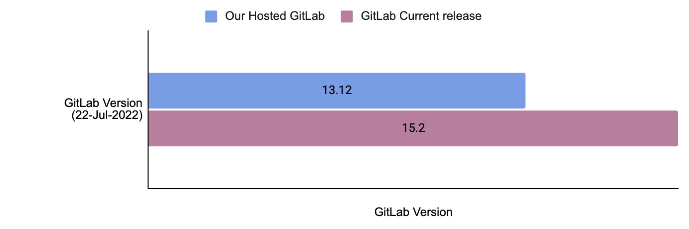
In a tech-driven field, staying updated isn’t an option—it’s essential. At Grab, we’re committed to providing top-notch technology services. However, keeping pace can be demanding. At one point in time, our GitLab instance was trailing by roughly 14 months of releases. This blog post recounts our experience updating and formulating a consistent upgrade routine.
Recognising the need to upgrade
Our team, while skilled, was still learning GitLab’s complexities. Regular stability issues left us little time for necessary upgrades. Understanding the importance of upgrades for our operations to get latest patches for important security fixes and vulnerabilities, we started preparing for GitLab updates while managing system stability. This meant a quick learning and careful approach to updates.
The following image illustrates the version discrepancy between our self-hosted GitLab instance and the official most recent release of GitLab as of July 2022. GitLab follows a set release schedule, issuing one minor update monthly and rolling out a major upgrade annually.
Fig 1. The difference between our hosted version and the latest available GitLab version by 22 July 2022
Addressing fears and concerns
We were concerned about potential downtime, data integrity, and the threat of encountering unforeseen issues. GitLab is critical for the daily activities of Grab engineers. It serves a critical user base of thousands of engineers actively using it, hosting multiple mono repositories with code bases ranging in size from 1GB to a sizable 15GB. When taking into account all its artefacts, the overall imprint of a monorepo can extend to an impressive 39TB.
Our self-hosted GitLab firmly intertwines with multiple critical components. We’ve aligned our systems with GitLab’s official reference architecture for 5,000 users. We use Terraform to configure complete infrastructure with immutable Amazon Machine Images (AMIs) built using Packer and Ansible. Our efficient GitLab setup is designed for reliable performance to serve our wide user base. However, any fault leading to outages can disrupt our engineers, resulting in a loss of productivity for hundreds of teams.
High-level GitLab Architecture Diagram
The above is the top level architecture diagram of our GitLab infrastructure. Here are the major components of the GitLab architecture and their functions:
Gitaly: Handles low-level Git operations for GitLab, such as interacting directly with the code repository present on disk. It’s important to mention that these code repositories are also stored on the same Gitaly nodes, using the attached Amazon Elastic Block Store (Amazon EBS) disks.
Praefect: Praefect in GitLab acts as a manager, coordinating Gitaly nodes to maintain data consistency and high availability.
Sidekiq: The background processing framework for GitLab written in Ruby. It handles asynchronous tasks in GitLab, ensuring smooth operation without blocking the main application.
App Server: The core web application server that serves the GitLab user interface and interacts with other components.
The importance of preparation
Recognising the complexity of our task, we prioritised careful planning for a successful upgrade. We studied GitLab’s documentation, shared insights within the team, and planned to prevent data losses.
To minimise disruptions from major upgrades or database migrations, we scheduled these during weekends. We also developed a checklist and a systematic approach for each upgrade, which include the following:
Diligently go through the release notes for each version of GitLab that falls within the scope of our upgrade.
Read through all dependencies like RDS, Redis, and Elasticsearch to ensure version compatibility.
Create documentation outlining new features, any deprecated elements, and changes that could potentially impact our operations.
Generate immutable AMIs for various components reflecting the new version of GitLab.
Revisit and validate all the backup plans.
Refresh staging environment with production data for accurate, realistic testing and performance checks, and validation of migration scripts under conditions similar to the actual setup.
Upgrade the staging environment.
Conduct extensive testing, incorporating both automated and manual functional testing, as well as load testing.
Conduct rollback tests on the staging environment to the previous version to confirm the rollback procedure’s reliability.
Inform all impacted stakeholders, and provide a defined timeline for upcoming upgrades.
We systematically follow GitLab’s official documentation for each upgrade, ensuring compatibility across software versions and reviewing specific instructions and changes, including any deprecations or removals.
The first upgrade
Equipped with knowledge, backup plans, and a robust support system, we embarked on our first GitLab upgrade two years ago. We carefully followed our checklist, handling each important part systematically. GitLab comprises both stateful (Gitaly) and stateless (Praefect, Sidekiq, and App Server) components, all managed through auto-scaling groups. We use a ‘create before destroy’ strategy for deploying stateless components and an ‘in-place node rotation’ method via Terraform for stateful ones.
We deployed key parts like Gitaly, Praefect, Sidekiq, App Servers, Network File System (NFS) server, and Elasticsearch in a specific sequence. Starting with Gitaly, followed by Praefect, then Sidekiq and App Servers, and finally NFS and Elasticsearch. Our thorough testing showed this order to be the most dependable and safe.
However, the journey was full of challenges. For instance, we encountered issues such as the Gitaly cluster falling out of sync for monorepo and the Praefect server failing to distribute the load effectively. Praefect assigns a primary Gitaly node for each repository to host it. All write operations are sent to the repository’s primary node, while read requests are spread across all synced nodes in the Gitaly cluster. If the Gitaly nodes aren’t synced, Praefect will redirect all write and read operations to the repository’s primary node.
Gitaly is a stateful application, we upgraded each Gitaly node with the latest AMI using an in-place node rotation strategy. In older versions of GitLab (up to v14.0), if a Gitaly node is unhealthy, Praefect would immediately update the primary node for the repository to any healthy Gitaly node. After the rolling upgrade for a 3-node Gitaly cluster, repositories were mainly concentrated on only one Gitaly node.
In our situation, a very busy monorepo was assigned to a Gitaly node that was also the main node for many other repositories. When real traffic began after deployment, the Gitaly node had trouble syncing the monorepo with the other nodes in the cluster.
Because the Gitaly node was out of sync, Praefect started sending all changes and access requests for monorepo to this struggling Gitaly node. This increased the load on the Gitaly server, causing it to fail. We found this to be the main issue and decided to manually move our monorepo to a Gitaly node that was less crowded. We also added a step to validate primary node distribution to our deployment checklist.
This immediate failover behaviour changed in GitLab version 14.1. Now, a primary is only elected lazily when a write request arrives for any repository. However, since we enabled maintenance mode before the Gitaly deployment, we didn’t receive any write requests. As a result, we did not see a shift in the primary node of the monorepo with new GitLab versions.
Regular upgrades: Our new normal
Embracing the practice of consistent upgrades dramatically transformed the way we operate. We initiated frequent upgrades and implemented measures to reduce the actual deployment time.
Perform all major testing in one day before deployment.
Prepare a detailed checklist to follow during the deployment activity.
Reduce the minimum number of App Server and Sidekiq Servers required just after we start the deployment.
Upgrade components like App Server and Sidekiq in parallel.
Automate smoke testing to examine all major workflows after deployment.
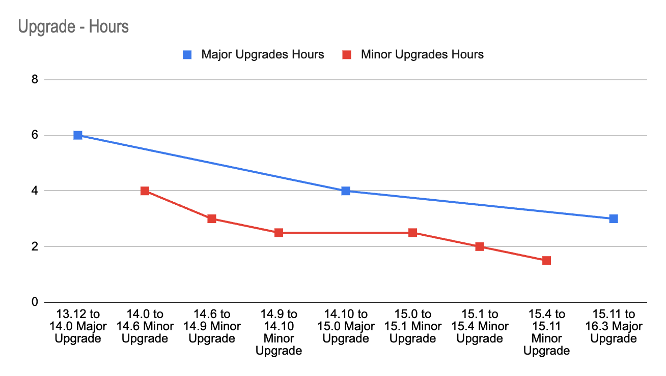
Leveraging the lessons learned and the experience gained with each upgrade, we successfully cut the time spent on the entire operation by 50%. The image-3 shows how we reduced our deployment time for major upgrades from 6 hours to 3 hours and our deployment time for minor upgrades from 4 to 1.5 hours.
Each upgrade enriched our comprehensive knowledge base, equipping us with insights into the possible behaviours of each component under varying circumstances. Our growing experience and enhanced knowledge helped us achieve successful upgrades with less downtime with each deployment.
Rather than moving up one minor version at a time, we learned about the feasibility of skipping versions. We began using the GitLab Upgrade Path. This method allowed us to skip several versions, closing the distance to the latest version with fewer deployments. This approach enabled us to catch up on 24 months’ worth of upgrades in just 11 months, even though we started 14 months behind.
Time taken in hrs for each upgrade. The blue line depicts major and the red line is for minor upgrades
Overcoming challenges
Our journey was not without hurdles. We faced challenges in maintaining system stability during upgrades, navigating unexpected changes in functionality post upgrades, and ensuring data integrity.
However, these challenges served as an opportunity for our team to innovate and create robust workarounds. Here are a few highlights:
Unexpected project distribution: During upgrades and Gitaly server restarts, we observed unexpected migration of the monorepo to a crowded Gitaly server, resulting in higher rate limiting. We manually updated primary nodes for the monorepo and made this validation as a part of our deployment checklist.
NFS deprecation: We migrated all required data to S3 buckets and deprecated NFS to become more resilient and independent of Availability Zone (AZ).
Handling unexpected Continuous Integration (CI) operations: A sudden surge in CI operations sometimes resulted in rate limiting and interrupted more essential Git operations for developers. This is because GitLab uses different RPC calls and their concurrency for SSH and HTTP operations. We encouraged using HTTPS links for GitLab CI and automation script and SSH links for regular Git operations.
Right-sizing resources: We countered resource limitations by right-sizing our infrastructure, ensuring each component had optimal resources to function efficiently.
Performance testing: We conducted performance testing of our GitLab using the GitLab Performance Tool (GPT). In addition, we used our custom scripts to load test Grab specific use cases and mono repositories.
Limiting maintenance windows: Each deployment required a maintenance window or downtime. To minimise this, we structured our deployment processes more efficiently, reducing potential downtime and ensuring uninterrupted service for users.
Dependency on GitLab.com image registry: We introduced measures to host necessary images internally, which increased our resilience and allowed us to cut ties with external dependencies.
The results
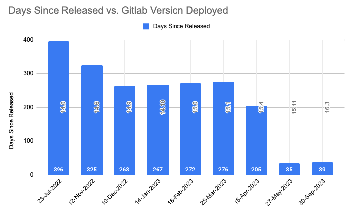
Through careful planning, we’ve improved our upgrade process, ensuring system stability and timely updates. We’ve also reduced the delay in aligning with official GitLab releases. The image below displays how the time delay between release date and deployment has been reduced with each upgrade. It sharply brought down from 396 days (around 14 months) to 35 days.
At the time of this article, we’re just two minor versions behind the latest GitLab release, with a strong focus on security and resilience. We are also seeing a reduced number of reported issues after each upgrade.
Our refined process has allowed us to perform regular updates without any service disruptions. We aim to leverage these learnings to automate our upgrade deployments, painting a positive picture for our future updates, marked by efficiency and stability.
Time delay between official release date and date of deployment
Looking ahead
Our dedication extends beyond staying current with the most recent GitLab versions. With stabilised deployment, we are now focusing on:
Automated upgrades: Our efforts extend towards bringing in more automation to enhance efficiency. We’re already employing zero-downtime automated upgrades for patch versions involving no database migrations, utilising GitLab pipelines. Looking forward, we plan to automate minor version deployments as well, ensuring minimal human intervention during the upgrade process.
Automated runner onboarding for service teams: We’ve developed a ‘Runner as a Service’ solution for our service teams. Service teams can create their dedicated runners by providing minimal details, while we manage these runners centrally. This setup allows the service team to stay focused on development, ensuring smooth operations.
Improved communication and data safety: We’re regularly communicating new features and potential issues to our service teams. We also ensure targeted solutions for any disruptions. Additionally, we’re focusing on developing automated data validation via our data restoration process.
Focus on development: With stabilised updates, we’ve created an environment where our development teams can focus more on crafting new features and supporting ongoing work, rather than handling upgrade issues.
Key takeaways
The upgrade process taught us the importance of adaptability, thorough preparation, effective communication, and continuous learning. Our ‘No Version Left Behind’ motto underscores the critical role of regular tech updates in boosting productivity, refining processes, and strengthening security. These insights will guide us as we navigate ongoing technological advancements.
Below are the key areas in which we improved:
Enhanced testing procedures: We’ve fine-tuned our testing strategies, using both automated and manual testing for GitLab, and regularly conducting performance tests before upgrades.
Approvals: We’ve designed approval workflows that allow us to obtain necessary clearances or approvals before each upgrade efficiently, further ensuring the smooth execution of our processes.
Improved communication: We’ve improved stakeholder communication, regularly sharing updates and detailed documents about new features, deprecated items, and significant changes with each upgrade.
Streamlined planning: We’ve improved our upgrade planning, strictly following our checklist and rotating the role of Upgrade Ownership among team members.
Optimised activity time: We’ve significantly reduced the time for production upgrade activity through advanced planning, automation, and eliminating unnecessary steps.
Efficient issue management: We’ve improved our ability to handle potential GitLab upgrade issues, with minimal to no issues occurring. We’re prepared to handle any incidents that could cause an outage.
Knowledge base creation and automation: We’ve created a GitLab knowledge base and continuously enhanced it with rich content, making it even more invaluable for training new team members and for reference during unexpected situations. We’ve also automated routine tasks to improve efficiency and reduce manual errors.
Join us
Grab is the leading superapp platform in Southeast Asia, providing everyday services that matter to consumers. More than just a ride-hailing and food delivery app, Grab offers a wide range of on-demand services in the region, including mobility, food, package and grocery delivery services, mobile payments, and financial services across 428 cities in eight countries.
Powered by technology and driven by heart, our mission is to drive Southeast Asia forward by creating economic empowerment for everyone. If this mission speaks to you, join our team today!
To provide the best experiences, we use technologies like cookies to store and/or access device information. Consenting to these technologies will allow us to process data such as browsing behavior or unique IDs on this site. Not consenting or withdrawing consent, may adversely affect certain features and functions.
Functional
Always active
The technical storage or access is strictly necessary for the legitimate purpose of enabling the use of a specific service explicitly requested by the subscriber or user, or for the sole purpose of carrying out the transmission of a communication over an electronic communications network.
Preferences
The technical storage or access is necessary for the legitimate purpose of storing preferences that are not requested by the subscriber or user.
Statistics
The technical storage or access that is used exclusively for statistical purposes.The technical storage or access that is used exclusively for anonymous statistical purposes. Without a subpoena, voluntary compliance on the part of your Internet Service Provider, or additional records from a third party, information stored or retrieved for this purpose alone cannot usually be used to identify you.
Marketing
The technical storage or access is required to create user profiles to send advertising, or to track the user on a website or across several websites for similar marketing purposes.


.jpg)