In March 2023, I embarked on a mission to explore the potential of Large Language Models (LLMs) within Grab. What started off as an attempt to solve a specific problem—reducing the burden on our ML Platform team’s support channels, ended up becoming something much bigger. The creation of GrabGPT, an internal ChatGPT-like tool that has transformed how folks in Grab interact with AI. This is the story of how a failed experiment led to one of Grab’s most impactful internal tools.
The problem: Overwhelmed support channels
As part of Grab’s machine learning platform team, we were drowning in user inquiries. Slack channels were flooded with questions and our on-call engineers were spending more time answering repetitive queries than building innovative solutions. This led me to ponder on this question, “could we use LLMs to build a chatbot that understands our platform’s documentation and answers these questions automatically?”
The first attempt: A chatbot for platform support
I started by exploring open-source frameworks to build a chatbot. I stumbled upon chatbot-ui, a simple yet powerful tool that could be wired up with LLMs. My idea was to feed the chatbot our platform’s Q\&A documentation (over 20,000 words) and let it handle user queries.
But there was a catch: GPT-3.5-turbo could only handle 8,000 tokens (~2,000 words). I spent days summarising the documentation, reducing it to less than 800 words. While the chatbot worked for a handful of frequently asked questions, it was clear that this approach wasn’t scalable. I tried with embedding search and it didn’t work that well too, so I decided to give up on this idea.
The pivot: Why not build Grab’s own ChatGPT?
As I stepped back, a new thought struck me: Grab doesn’t have its own ChatGPT-like tool yet. I had the frameworks, the LLM knowledge, and most importantly—access to Grab’s model-serving platform, catwalk. Why not build an internal tool that any Grabber could use?
Over a weekend, I extended the existing frameworks, added Google login for authentication, and deployed the tool internally. I called it Grab’s ChatGPT. Little did I know, this would become one of the most widely used tools in the company.
The tool quickly became a staple for Grabbers, especially in regions where ChatGPT was inaccessible (e.g., China). The name evolved too—our PM suggested GrabGPT, and it stuck.
The Success: GrabGPT takes off
The response was overwhelming:
Day 1: 300 users registered.
Day 2: 600 new users.
Week 1: 900 new users
Month 3: Over 3000 users, with 600 daily active users
Today: Almost all Grabbers are using GrabGPT.
Figure 1: Number of GrabGPT users in one month
Why GrabGPT works: More than just technology
The success of GrabGPT isn’t just about the tech,it’s about timing, security, and accessibility. Here’s why it resonated so deeply within Grab:
Data security: GrabGPT operates on a private route, ensuring that sensitive company data never leaves our infrastructure.
Global accessibility: Unlike ChatGPT, which is banned in some regions, GrabGPT is accessible to all Grabbers, regardless of location.
Model agnosticism: GrabGPT isn’t tied to a single LLM provider. It supports models from OpenAI, Claude, Gemini, and more.
Auditability: Every interaction on GrabGPT is auditable, making it a favorite of our data security and governance teams.
The broader impact: A catalyst for LLM strategy
GrabGPT didn’t just solve an immediate problem, it sparked a broader conversation about how LLMs can be leveraged across Grab. It showed that a single engineer, provided with the right tools and timing, can create something transformative. Today, GrabGPT is more than a tool; it’s a testament to the power of experimentation and adaptability.
Lessons learned
Failure is a stepping stone: My initial failure with the support chatbot which then led me to a much bigger opportunity.
Timing matters: GrabGPT succeeded because it addressed a critical need at the right time.
Think big, start small: What began as a weekend project became a company-wide tool.
Collaboration is key: The enthusiasm and contributions from other Grabbers were instrumental in scaling GrabGPT.
Conclusion
GrabGPT is a story of resilience, innovation, and the unexpected rewards from thinking outside the box. It’s a reminder that sometimes, the best solution comes from pivoting away from what doesn’t work and embracing new possibilities. As LLMs continue to evolve, I’m excited to see how GrabGPT will grow and inspire even more innovation within Grab.
I would like to end this article by letting readers know that if you’re working on a project and feel stuck, don’t be afraid to pivot. You never know, your next failure might just be the beginning of your greatest success. And if you’re at Grab, give GrabGPT a try. It might just change the way you work!
Join us
Grab is a leading superapp in Southeast Asia, operating across the deliveries, mobility and digital financial services sectors. Serving over 800 cities in eight Southeast Asian countries, Grab enables millions of people everyday to order food or groceries, send packages, hail a ride or taxi, pay for online purchases or access services such as lending and insurance, all through a single app. Grab was founded in 2012 with the mission to drive Southeast Asia forward by creating economic empowerment for everyone. Grab strives to serve a triple bottom line – we aim to simultaneously deliver financial performance for our shareholders and have a positive social impact, which includes economic empowerment for millions of people in the region, while mitigating our environmental footprint.
Powered by technology and driven by heart, our mission is to drive Southeast Asia forward by creating economic empowerment for everyone. If this mission speaks to you, join our team today!
At Grab, we operate a set of services that manage and provide counts of various items. While this may seem straightforward, the scale at which this feature operates—benefiting millions of Grab users daily—introduces complexity. This feature is divided into three microservices: one for “writing” counts, another for handling “read” requests, and a third serving as the backend for a portal used by data scientists and analysts to configure these counters.
This article focuses on the service responsible for handling “read” requests. This service is backed by Scylla storage and a Redis cache. It also connects to a MySQL RDS to retrieve “counter configurations” that are necessary for processing incoming requests. Written in Rust, the service serves tens of thousands of queries per second (QPS) during peak times, with each request typically being a “batch request” requiring multiple lookups (~10) on Scylla.
Recently, the service has encountered performance challenges, causing periodic spikes in Scylla QPS. These spikes occur throughout the day but are particularly evident during peak hours. To understand this better, we’ll first walk you through how this service operates, particularly how it serves incoming requests. We will then explain our proposed solution and the outcomes of our experiment.
Anatomy of a request
Each counter configuration stored in MySQL has a template that dictates the format of incoming queries. For example, this sample counter configuration is used to count the raindrops for a specific city:
An incoming request using this counter might look like this:
{
    "key": "rain_drops:city:111222",
    "fromTime": 1727215430, // 24 September 2024 22:03:50
    "toTime": 1727400000, // 27 September 2024 01:20:00
}
This request seeks the number of raindrops in our imaginary city with city ID: 111222, between 1727215430 (24 September 2024 22:03:50) and 1727400000 (27 September 2024 01:20:00).
Another service keeps track of raindrops by city and writes the minutely (truncated at 15 minutes), hourly, and daily counts to three different Scylla tables:
minutely_count_table
hourly_count_table
daily_count_table
The service processing the request rounds down the time to the nearest 15 minutes. As a result, the request is processed with the following time range:
Start time: 24 September 2024 22:00:00
End time: 27 September 2024 01:15:00
Let’s assume we have the following data in these three tables for “rain_drops:city:111222”. The datapoints used in the above example request are highlighted in bold.
minutely_count_table:
key
minutely_timestamp
count
rain_drops:city:111222
2024-09-24T22:00:00Z
3
rain_drops:city:111222
2024-09-24T22:15:00Z
2
rain_drops:city:111222
2024-09-24T22:30:00Z
4
rain_drops:city:111222
2024-09-24T22:45:00Z
1
…
…
…
rain_drops:city:111222
2024-09-27T01:00:00Z
2
rain_drops:city:111222
2024-09-27T01:15:00Z
3
hourly_count_table:
key
hourly_timestamp
count
rain_drops:city:111222
2024-09-24T22:00:00Z
18
rain_drops:city:111222
2024-09-24T23:00:00Z
22
rain_drops:city:111222
2024-09-25T00:00:00Z
15
…
…
…
rain_drops:city:111222
2024-09-27T00:00:00Z
11
rain_drops:city:111222
2024-09-27T01:00:00Z
9
daily_count_table:
key
daily_timestamp
count
rain_drops:city:111222
2024-09-24T00:00:00Z
214
rain_drops:city:111222
2024-09-25T00:00:00Z
189
rain_drops:city:111222
2024-09-26T00:00:00Z
245
rain_drops:city:111222
2024-09-27T00:00:00Z
78
Now, let’s see how the service calculates the total count for the incoming request with “rain_drops:city:111222” based on the provided data:
Time range:
From: 24 September 2024 22:03:50
To: 27 September 2024 01:20:00
For the full days within the range, specifically 25th and 26th September, we can use data from the daily_count_table. However, for the start (24th September) and end (27th September) date of the range, we cannot use data from the daily_count_table as the range only includes portions of these dates. Instead, we will use a combination of data from the hourly_count_table and minutely_count_table to accurately capture the counts for these days.
Query the daily_count_table:
Sum (full day: 25 and 26th Sep): 189 + 245 = 434
Query the hourly_count_table:
For 24th September (from 22:00:00 to 23:59:59):
Hourly count: 18 + 22 = 40
For 27th September (from 00:00:00 to 01:00:00):
Hourly count: 11
Query the minutely_count_table:
For 27th September (from 01:00:00 to 01:15:00):
Minutely count: 2
Total count:
Total = Daily count (25th and 26th) + Hourly count (24th) + Hourly count (27th) + Minutely count (27th)
= 434 + 40 + 11 + 2
= 487
Figure 1: The example request for “rain_drops:city:111222” is handled using data from three different Scylla tables.
As shown in the calculation, when the service receives the request, it comes up with the total count of raindrops by querying three Scylla tables and summing them up using some specific rules within the service itself.
Querying the cache
In the previous section, we explained how Scylla handles a query. If we cached the response for the same request earlier, retrieval from the cache follows a simpler logic. For instance, for the example request, the total count is stored using the floored start and end times (rounded to the nearest 15-minute window within an hour), which was used for the Scylla query instead of the original time in the request. The cache key-value pair would look like this:
Timestamps 1727215200 and 1727399700 represent the adjusted start and end times of 24 September 2024 22:00:00 and 27 September 2024 01:15:00, respectively. It has a Time-To-Live (TTL) of 5 minutes. During this TTL window, any request for the key “rain_drops:city:111222” having the same start and end times (after rounding to the nearest 15 minutes) will be read from the cache instead of querying Scylla.
For example, for the following three start times, although they are different, after flooring the request to the nearest 15 minutes, the start time becomes 24 September 2024 22:00:00 for all of them, which is the same start time as the one in the cache.
24 September 2024 22:01:00
24 September 2024 22:02:00
24 September 2024 22:06:00
In day-to-day operations, this caching setup allows roughly half of our total production requests to be served by the Redis cache.
Figure 2. The graph visualises the relative quantity of cache hits vs Scylla-bound requests.
Problem statement
The setup consisting of Scylla and Redis cache works well. Particularly because Scylla-bound queries need to look up 1-3 tables (minutely, hourly, daily, depending on the time range) and perform the summation as explained earlier, whereas a single cache lookup gets the final value for the same query. However, as our cache key pattern follows the 15-minute truncation strategy, along with a 5-minute cache TTL, it leads to an interesting phenomenon – our cache hits plummet and Scylla QPS spikes at the end of every 15 minutes.
Figure 3. Graph showing 15-minute spikes in Scylla-bound requests accompanied by a decline in cache hit rates.
This occurs primarily due to the fact that almost all requests to our service are for recent data. Due to this, at the end of every 15-minute block within an hour (i.e., 00, 15, 30, 45), most of the requests require creating new cache keys for the latest 15-minute block. At this point in time, there may be many unexpired (i.e., have not reached 5 min TTL) cache keys from the previous 15-minutes block, but they become less relevant as most requests are asking for recent data.
The table in Figure 4 shows example data for configurations “rain_drops:city:111222” and “bird_sighting:city:333444”. For these two configurations, new cache keys are created due to TTL expiry at random times. However, at the end of the 15-minute block, which, in this case is at the end of 22:00-22:15 block, both configurations need new cache keys for the new 15-minute time block that has just started (i.e., start of 22:15-22:30), even though some of their cache keys from the previous 15-minute block are still valid. This requirement of creating new cache keys for most of the requests at the end of a 15-minute block causes spikes in Scylla QPS and a sharp decline in cache hits.
One question that arises is – “Why don’t we see a spike every 5 minutes for cache key TTL expiry?” This is because, within the 15 minutes block, new cache keys are continuously created when a key reaches TTL and a new request for that is received. Since this happens all the time as shown in Figure 4, we do not see a sharp spike. In other words, although Scylla does receive more queries due to cache TTL expiry, it does not lead to a spike in Scylla queries or a sharp drop in cache hits. This is because the cache keys are always being created and invalidated due to TTL expiry instead of following a fixed 5-minute block similar to the 15-minute block we use for our truncation strategy.
Figure 4. This table visualises scenarios when new cache keys are required due to TTL expiry vs due to 15-minute truncation strategy.
These Scylla QPS spikes at the end of every 15-minute block lead to a highly imbalanced Scylla QPS. This often causes high latency in our service during the 15-minute blocks that fall within the peak traffic hours. This further causes more requests to time out, eventually increasing the number of failed requests.
Proposed solution
We propose mitigating this issue by completely removing the Redis-backed caching mechanism from the service. Our observations indicate that the Scylla spikes at the end of 15-minute blocks occur due to cache hit misses. Therefore, removing the caching should eliminate the spikes and provide for a more balanced load.
We acknowledge that this may seem counterintuitive from an overall performance standpoint as removing caching means all queries will be Scylla-bound, potentially impacting the overall performance since caching usually speeds up processes. In addition, caching also comes with an advantage where for cache hits, the service does not need to do the summation on Scylla results from minutely, hourly, and the daily table. Despite these shortcomings, we hypothesise that removing caching should not have an adverse impact on the overall performance. This is based on the fact the Scylla has its own sophisticated caching mechanism. However, our existing setup uses Redis for caching, underutilising Scylla’s cache as the most subsequent queries hit the Redis cache instead.
In summary, we propose eliminating the Redis caching component from our current architecture. This change is expected to resolve the Scylla query spikes observed at the end of every 15-minute block. By relying on Scylla’s native caching mechanism, we anticipate maintaining the service’s overall performance more effectively. The removal of Redis is counterbalanced by the optimised utilisation of Scylla’s built-in caching capabilities.
Experiment
Procedure
The experiment was done on an important live service serving thousands of QPS. To avoid disruptions, we followed a gradual approach. We first turned off caching for a few configurations. If there were no adverse impacts observed, we incrementally disabled cache for more configurations. We controlled the rollout increment by using a mathematical operator on the configuration IDs. This approach is simple and allows us to deterministically disable the cache for specific configurations across all requests, as opposed to using a percentage rollout which randomly disables the cache for different configurations across different requests. This is also due to the fact that the number of configurations is relatively steady and small (less than a thousand). Since these configurations are already fully cached in the service memory from RDS, there will be no performance impact of having a condition that operates on these configurations.
To make sense of the graphs and metrics reported in this section, it is important to understand the traffic pattern of this service. The service usually sees two peaks every day: noon and another around 6-7 PM. On a weekly basis, we usually see the highest traffic on Friday, with the busiest period being from 6-8 PM.
In addition, the timeline of when and how we made various changes to our setup is important to accurately interpret our results.
Experiment timeline: Nov 5 – Nov 13, 2024:
Redis cache disabled for ~5% of the counter configurations – Nov 5, 2024, 10.26 AM (Canary started: 10.00 AM)
Redis cache disabled for ~25% of the counter configurations – Nov 5, 2024, 12.44 PM (Canary started: 12.20 PM)
Redis cache disabled for ~35% of the counter configurations – Nov 6, 2024, 10.50 AM (Canary started: 10.21 AM)
Redis cache disabled for ~75% of the counter configurations – Nov 7, 2024, 10.53 AM (Canary started: 10.26 AM)
Experimenting with running a major compaction job during the day time: Tue, Nov 12, 2024, between 2-5 PM (on all nodes)
Day time scheduled major compaction job starts from: Tue, Nov 13, 2024, between 2-5 PM (on all nodes)
Redis cache disabled for 100% of the counter configs – Wed, 13 Nov 2024, 10:56 AM (Canary started: 10:32 AM)
Unless otherwise specified, the graphs and metrics we report in this article uses this fixed time window: Oct 31 (Thu) 12.00 AM – Nov 15 (Friday) 11.59 PM SGT. This time window covers the entire experiment period with some buffer to observe the experiment’s impact.
Observations
As we progressively disabled read from external Redis cache over the span of 8 days (Nov 5 – Nov 13), we made interesting observations and experimented with some Scylla configuration changes on our end. We describe them in the following sections.
Scylla hit vs. cache hit
As we progressively disabled Redis cache for most of the counters, one obvious impact was the gradual increase in Scylla-bound QPS and similar decrease in Redis-cache hit. When Redis-cache was enabled for 100% of the configurations, 50% of the requests were bound for Scylla and the other 50% were for Redis. At the end of the experiment, after fully disabling Redis cache, 100% of the requests were Scylla-bound.
Figure 5. Gradual increase in Scylla QPS and simultaneous decrease in Redis cache hit.
15-minutes and hourly spikes
We noticed that the 15-minute spikes in Scylla QPS as well as the associated latency slowly became less prominent and eventually disappeared from the graph after we completely disabled the Redis cache. However, we noticed that the hourly spike still remained. This is attributed to the higher QPS from the clients calling this service at the turn of every hour. As a result, limited optimisation can be done to reduce the hourly spike on this service’s end.
Figure 6. The 15-minute spikes in Scylla QPS disappeared after the external Redis cache was fully disabled. This graph uses a smaller time window to show the earlier spikes. It also shows the persistence of hourly spikes after the experiment which is attributed to the clients of this service sending more requests at the start of every hour.
Figure 7. The graph shows that the 15-minute spikes in Scylla’s latency disappeared after the external Redis cache was fully disabled. This graph uses a smaller time window to show the earlier spikes. It also shows the persistence of hourly spikes in latency after the experiment which is attributed to the clients of this service sending more requests at the start of every hour.
Service latency and additional Scylla compaction job
When we disabled Redis cache for about 75% of the counters configurations on Nov 7 (which accounts for about 85% of the overall QPS), we noticed an increase in the overall average service latency, from between 6-8 ms to 7-12 ms (P99 went from ~30-50ms to ~30-70ms). This caused a spike in open circuit breaker (CB) events on Hystrix. At this point, before disabling cache for more counters, on Nov 12, we experimented with running an additional major compaction job on Scylla between 2-5 PM on all our Scylla nodes, progressively on each availability zone (AZ). It is noteworthy that we already have a scheduled major compaction job that runs around 3 AM every day. The outcome of this experiment was quite positive. It brought back the average and P99 latency almost to the prior level when we had Redis cache enabled for 100% of the counters. This also had a similar effect on the Hystrix CB open events. Based on this observation, we made this additional day time major compaction job as a daily scheduled job. We disabled Redis cache for 100% of the counters the next day (Nov 13). This expectedly increased the Scylla QPS, with no noticeable adverse effect on the service latency or Hystrix CB open events.
Figure 8. This graph shows how the average latency changed as a result of the experiment. The higher spikes correspond to the time when Redis cache was being progressively disabled before introducing the day time Scylla compaction job. The spikes lessened after the compaction job was introduced on Nov 12 (Note: Friday spike was due to higher traffic in general).
Figure 9. This graph shows how the P99 latency changed as a result of the experiment. The higher spikes correspond to the time when Redis cache was being progressively disabled before introducing the day time Scylla compaction job. The spikes lessened after the compaction job was introduced on Nov 12 (Note: Friday spike was due to higher traffic in general).
Scylla’s own cache
One of our hypotheses was that we were not using Scylla cache due to our system’s design, along with all the service specific characteristics discussed earlier. Our experimental results show that this is indeed the case. We observed a significant increase in Scylla reads with Scylla’s own cache hits, while Scylla reads with Scylla’s own cache misses remained about the same despite our Scylla cluster receiving double the traffic. Percentage-wise, before disabling the external Redis cache, Scylla hit its own cache for ~30% of the total reads, and after we have completely disabled the external Redis cache, Scylla hit its cache for about 70% of the reads. We believe that this largely contributes to the overall performance of the service despite fully decommissioning the expensive Redis cache component from our system architecture.
Figure 10. Significant increase in Scylla reads after disable Redis cache.
Figure 11. No change in Scylla cache miss despite the doubling of Scylla traffic.
Scylla CPU and memory usage
Contrary to our assumption, although the Scylla QPS doubled due to the change done as part of this experiment, there was marginal increase in Scylla CPU usage (from ~50% to ~52% at peak). In terms of memory, Scylla log-structured allocator (LSA) memory usage remains consistent. For Non-LSA memory, the maximum utilisation did not increase. However, we noticed two daily spikes instead of one existed before the experiment. The second spike results from the newly added daily major compaction job. Notably,the overall non-LSA peak has slightly decreased after the introduction of the new compaction job.
Figure 12. Relatively steady Scylla CPU utilisation.
Figure 13. Non-LSA memory usage spikes twice a day after the experiment. The new spike corresponds to the newly added day time compaction job.
Conclusion
In summary, we were able to maintain the same service performance while removing an expensive Redis cache component from our system architecture, which accounted for about 25% of the overall service cost. This has been made possible primarily by significant increase in the utilisation of Scylla’s own cache and adding a daily major compaction job on all our Scylla nodes.
In the future, we plan to further experiment with different Scylla configurations for potential performance gain, specifically to improve the latency.
Join us
Grab is a leading superapp in Southeast Asia, operating across the deliveries, mobility and digital financial services sectors. Serving over 800 cities in eight Southeast Asian countries, Grab enables millions of people everyday to order food or groceries, send packages, hail a ride or taxi, pay for online purchases or access services such as lending and insurance, all through a single app. Grab was founded in 2012 with the mission to drive Southeast Asia forward by creating economic empowerment for everyone. Grab strives to serve a triple bottom line – we aim to simultaneously deliver financial performance for our shareholders and have a positive social impact, which includes economic empowerment for millions of people in the region, while mitigating our environmental footprint.
Powered by technology and driven by heart, our mission is to drive Southeast Asia forward by creating economic empowerment for everyone. If this mission speaks to you, join our team today!
The transformative world of Generative AI (GenAI), which refers to artificial intelligence systems capable of creating new content such as text, images, or music that is similar to human-generated content, has become integral to innovation, powering the next generation of AI-enabled applications. At Grab, it is crucial that every Grabber has access to these cutting-edge technologies to build powerful applications to better serve our customers and enhance their experiences. Grab’s AI Gateway aims to provide exactly this. The gateway seamlessly integrates AI providers like OpenAI, Azure, AWS (Bedrock), Google (VertexAI) and many other AI models, to bring seamless access to advanced AI technologies to every Grabber.
Why do we need Grab AI Gateway?
Before we begin implementing Grab AI Gateway in our work process, it is important for us to understand the limitations as well as the solutions that Grab AI Gateway provides. Failure to properly implement Grab AI Gateway could lead to roadblocks in development which negatively affect user experience.
Streamline access
Each AI provider has its own way of authenticating their services. Some providers use key-based authentication while others require instance roles or cloud credentials. Grab AI Gateway provides a centralised platform that only requires a one-time provider access setup. Grab AI Gateway removes the effort of procuring resources and setting up infrastructure for AI services, such as servers, storage, and other necessary components.
Enables experimentation
By providing a simple unified way to access different AI providers, users can experiment with various Large Language Models (LLMs) and choose the one best suited for their task.
Cost-efficient usage
Many AI providers allow purchasing of reserved capacity to provide higher throughput and improve cost effectiveness. However, services that require reservation or pre-purchases over a commitment period can lead to wastage.
Grab AI Gateway overcomes this problem and minimises wastage with a shared capacity pool. A deprecated service would simply free up bandwidth for a new service to utilise. Additionally, Grab AI Gateway provides a global view of usage trends to help platform teams make informed decisions on reallocating reserved capacity according to demand and future trends (eg. an upcoming model replacing an old one).
Auditing
A central setup ensures that use cases undergo a thorough review process to comply with the privacy and cyber security standards before being deployed in production. For instance, a Q&A bot with access to both restricted and non-restricted data could inadvertently reveal sensitive information if authorisation is not set up properly. Therefore, it is important that use cases are reviewed to ensure they follow Grab’s standard for data privacy and protection.
Platformisation benefits
Proper implementation of a central gateway provides platformisation benefits like:
Reduced operational costs.
Centralised monitoring and alerts.
Cost attribution.
Control limits like maximum QPS and cost cap.
Enforce guardrail and safety from prompt injection.
Architecture and design
At its core, the AI Gateway is a set of reverse proxies to different external AI providers like Azure, OpenAI, AWS, and others. From the user’s perspective, the AI Gateway acts like the actual provider where users are only required to set the correct base URLs to access the LLMs. The gateway handles functionalities like authentication, authorisation, and rate limiting, allowing users to solely focus on building GenAI enabled applications.
To form the basis of identity and access management (IAM) in the gateway, API key can be requested by the user for exploration (short-term personal key) or production (long-term service key) usage. The gateway implements a request path based authorisation where certain keys can be granted access to specific providers or features. Once authenticated, the AI Gateway replaces the internal key in request with the provider key and executes the request on behalf of the user.
The AI Gateway is designed with a minimalist approach, often serving as a lightweight interface between the user and the provider, intervening only when necessary. This has enabled us to keep up with the pace of innovation in the field and to continue expanding the provider catalogue without increasing the ops burden. Similar to requests, responses from the provider are returned to the user with no to minimal processing time. The gateway is not limited to only chat completion API. It exposes other APIs like embedding, image generation, and audio along with functionalities like fine-tuning, file storage, search, and context caching. The gateway also provides access to in-house open source models. This provides a taste of open source software (OSS) capabilities that users can later decide to deploy a dedicated instance using Catwalk’s VLLM offering.
Figure 1: High level architecture of AI Gateway
User journey and features
Onboarding process
GenAI based applications come with inherent risks like generating offensive or incorrect output and hostile takeover by malicious actors. As software practices and security standards for building GenAI applications are still evolving, it is important for users to be aware of the potential pitfalls. As AI Gateway is the de facto way to access this technology, the platform team shares the responsibility of building such awareness and ensuring compliance. The onboarding process includes a manual review stage. Every new use case requires a mini-RFC (Request For Comments) and a checklist that is reviewed by the platform team. In certain cases, an in-depth review by the AI Governance task force may be requested. To reduce friction, users are encouraged to build prototypes and experiment with APIs using “exploration keys”.
Exploration keys
At Grab, every Grabber is encouraged to use GenAI technologies to improve productivity and to experiment and learn within this field. The gateway provides exploration keys to make it easier for users to experiment with building chatbots and Retrieval Augmented Generation (RAG). These keys can be requested by Grabbers through a Slack bot. The keys are short-lived with a validity period of a few days, stricter rate limit restrictions, and access limited to only the staging environment. Exploration keys are highly popular, with more than 3,000 Grabbers requesting the key to experiment with APIs.
Unified API interface
In addition to provider specific interface, the gateway also offers a single interface to interact with multiple AI providers. For users, this lowers the barrier of experimenting between different providers/models, as they do not need to learn and rewrite their logic for different SDKs. Providers can be switched simply by changing the “model” parameter in the API request. This also enables easy setup of fallback logic and dynamic routing across providers. Based on popularity, the gateway uses the OpenAI API scheme to provide the unified interface experience. The API handler translates the request payload to the provider specific input scheme. The translated payload is then sent to reverse proxies. The returned response is translated back to the OpenAI response scheme.
Figure 2: Unified Interface Logic
Dynamic routing
The AI Gateway plays a crucial role in maintaining usage efficiency of various reserved instance capacities. It provides the control points to dynamically route requests for certain models to a different albeit similar model backed by a reserved instance. Another frequent use case is smart load balancing across different regions to address region-specific constraints related to maximum available quotas. This approach has helped to minimise rate limiting.
Auditing
The AI Gateway records each call’s request, response body, and additional metadata like token usage, URL path, and model name into Grab’s data lake. The purpose of doing so is to maintain a trail of usage which can be used for auditing. The archived data can be inspected for security threats like prompt injection or potential data policy violations.
Cost attribution
Allocating costs to each use case is important to encourage responsible usage. The cost of calling LLMs tends to increase at higher request rates, therefore understanding the incurred cost is crucial to understanding the feasibility of a use case. The gateway performs cost calculations for each request once the response is received from the provider. The cost is archived in the data lake along with an audit trail. For async usages like fine-tuning and assisting, the cost is calculated through a separate daily job. Finally, a job aggregates the cost for each service which is used for reporting on dashboards and showback. In addition, alerts are configured to notify if a service exceeds the cost threshold.
Rate limits
AI Gateway enforces its own rate limit on top of the global provider limits to make sure quotas are not consumed by a single service. Currently, limits are enforced on the request rate at the key level.
Integration with the ML Platform
At Grab, the ML platform serves as a one-stop shop, facilitating each phase of the model development lifecycle. The AI Gateway is well integrated with systems like Chimera notebooks used for ideation/development to Catwalk for deployment. When a user spins up a Chimera notebook, an exploration key is automatically mounted and is ready for use. For model deployments, users can configure the gateway integration which sets up the required environment variables and mounts the key into the app.
Challenges faced
With more than 300 unique use cases onboarded and many of those making it to production, AI Gateway has gained popularity since its inception in 2023. The gateway has come a long way, with many refinements made to the UX and provider offerings. The journey has not been without its challenges. Some of the challenges have become more prominent as the number of apps deployed increases.
Keeping up with innovations
With new features or LLMs being released at a rapid pace, the AI Gateway development has required continuous dedicated effort. Reflecting on our experience, it is easy to get overwhelmed by a constant stream of user requests for each new development in the field. However, we have come to realise it is important to balance release timelines and user expectations.
Fair distribution of quota
Every use case has a different service level objective (SLO). Batch use cases require high throughput but can tolerate failures while online applications are sensitive to latency and rate limits. In many cases, the underlying provider resource is the same. The responsibility falls over to the gateway to ensure fair distribution based on criticality and requests per second (RPS) requirements. As adoption increases, we have encountered issues where batch usage interfered with the uptime of online services. The use of Async APIs does mitigate the issues, but not all use cases can adhere to turnaround time.
Maintaining reverse proxies
Building the gateway as a reverse proxy was a key design decision. While the decision has proven to be beneficial, it is not without its complexity. The design ensures that the gateway is compatible with provider-specific SDKs. However, over time, we have encountered edge cases where certain SDK functionalities do not work as expected due to a missing path in the gateway or a missing configuration. These issues are usually ironed out when caught and a suite of integration tests with SDKs are conducted to ensure there are no breaking changes before deploying.
Current use cases and applications
Today, the gateway powers many AI-enabled applications. Some examples include real time audio signal analysis for enhancing ride safety, content moderation to block unsafe content, and description generator for menu items and many others.
Internally, the gateway powers innovative solutions to boost productivity and reduce toil. A few examples are:
GenAI portal that is used for translation and language detection tasks, image generation, and file analysis.
Text-to-Insights for converting questions into SQL queries.
Incident management automation for triaging incidents and creating reports.
Support bot for answering user queries in Slack channels using a knowledge base.
What’s next?
As we continue to add more features, we plan to focus our efforts on these areas:
1. Catalogue
With over 50 AI models each suited for a specific task type, finding the correct model to use is becoming complex. Users are often unsure of the difference between models in terms of capabilities, latency, and cost implications. A catalogue can serve as a guideline by listing currently supported models along with the list of metadata like the input/output modality, token limits, provider quota, pricing, and reference guide.
2. Out of box governance
Currently, all AI-enabled services that process clear text input and output from customers require users to set up their own guardrails and safety measures. By creating a built-in support for security threats like prompt injection and guardrails for filtering input/output, we can save users significant effort.
3. Smarter rate limits
At the current time, the gateway supports basic request rate-based limits at key level. While this rudimentary offering has been proven useful, it has its limitations. More advanced rate limiting policies based on token usage or daily/monthly running costs should be introduced to enforce better and fairer limits. These policies can be modified to be applied on different models and providers.
Special thanks to Priscilla Lee, Isella Lim, and Kevin Littlejohn for helping us in the project and Padarn Wilson for his leadership.
Join us
Grab is the leading superapp platform in Southeast Asia, providing everyday services that matter to consumers. More than just a ride-hailing and food delivery app, Grab offers a wide range of on-demand services in the region, including mobility, food, package and grocery delivery services, mobile payments, and financial services across 700 cities in eight countries.
Powered by technology and driven by heart, our mission is to drive Southeast Asia forward by creating economic empowerment for everyone. If this mission speaks to you, join our team today!
Welcome to the behind-the-scenes story of GrabUnlimited, Grab’s flagship membership program. We undertook the mammoth task of migrating from our legacy system to a Temporal1 workflow-based system, enhancing our ability to handle millions of subscribers with increased efficiency and resilience. The result? A whopping 80% reduction in open production incidents, and most importantly – an improved membership experience for our users. In this first part of the series, you will learn how to design a robust and scalable membership system as we delve into our own experience building one.
What is GrabUnlimited?
The idea behind GrabUnlimited, is pretty simple: you pay a monthly fee, you get monthly benefits as a member (e.g discounted food delivery fee). A membership system plays a key role in enhancing user experience by giving them more value for money, but also by building loyalty, making Grab their go-to app for everyday needs. However, as this program grew and evolved, it brought along unique challenges and opportunities.
With the initial triumph and significant surge in subscriber count by over 1000% from January 2022 to June 2023 – which we were super proud of! – the architecture that supported GrabUnlimited was starting to show signs of strain. Common subscriber concerns such as not receiving their membership benefits, along with developer issues marked by an increase in service outages highlighted the system’s low resiliency. The culprit? A backend service that, while functional, was not built to efficiently manage the complexities of a rapidly scaling membership model.
Deep dive into our previous system design
As engineers, we know that deciding to migrate any system to a new one is like changing the engine of a running car. It requires meticulous evaluation of the existing systems, a deep dive into the issues and their root causes, and a thorough analysis of potential solutions and their trade-offs.
How was GrabUnlimited designed?
Initially, GrabUnlimited systems were designed for an experiment and not a full-fledged regional product. The idea was to try it out as a minimum viable product over a restricted segment of a few hundred thousand users. Let’s first have a look at how the membership program works.
Figure 1. GrabUnlimited life of a membership flowchart.
Under the hood, our membership system relies on two main flows
Membership purchase: The user enrols for a certain duration (e.g 3 months), completes the payment through our Payment service, and receives benefits via our Reward service.
Membership renewal: A daily cron job2 checks which memberships need renewal, processes the payment, and delivers the benefits.
We employed a state machine3 approach to break down the membership process into smaller chunks called state handlers. For instance, a membership might transition through ‘Init’, ‘Charged’, ‘Rewarded’, and ‘Active’ states. To operate these states, we used Amazon’s Simple Queue Service (SQS). SQS acts as a manager, delegating state handlers to workers (our service) and monitoring the status of the state handler. If a worker fails to complete a task, SQS reassigns the task to another worker, ensuring no task is lost. The load is also spread across multiple workers, helping with scalability.
To safeguard our system against duplicate tasks such as charging the user twice, when a worker takes up a task, it would use a Redis lock4 mechanism with a time-to-live (TTL) of five minutes preventing any other worker from picking up the same task. If a worker fails or crashes, the lock expires and another worker can pick up the job.
So far, so good.
Figure 2. GrabUnlimited previous system design overview.
With our success came many challenges
As our subscriber base grew, we experienced an increase in system outages. To address this, we scrutinised metrics like the number of support tickets and gauged the toll on our engineering team. This included the time spent patching up issues and the opportunity cost of not developing new features or improvements.
From our subscribers’ point of view, we saw a steady increase in reported incidents.
Users were blocked because their membership status was corrupted in our database.
Memberships were not automatically renewed, or users were not able to resubscribe.
Users were not receiving their benefits after renewing their membership.
From the engineering team’s perspective, we were dedicating one engineer every week to battle these incidents full time. The on-call engineers were not only tasked with manually fixing all customer reports but were also swamped with frequent system alerts. This situation had three detrimental impacts on our team:
We were constantly putting out fires instead of addressing the root causes.
We were spending resources that could have been used to enhance our customers’ experience.
Our team’s motivation and confidence was taking a big hit.
Finding the architectural culprit
The first step was to clearly identify and understand the issues within our systems. We looked at the frequency of failures and their root cause. From there, we were able to detect recurring patterns, which led us to four major issues in our architecture.
Scalability
Our system’s cron job, which retrieves all daily memberships due for renewal from our database, becomes slower and more resource-intensive as the number of members increases. Despite our attempt to alleviate high database usage by dividing the process into multiple batches and running several cron jobs, we were still experiencing significant surges each time a cron job runs. So our only viable solution was vertical scaling5 of the database. In other words, we had a serious bottleneck in our system.
Figure 3. Database queries per second during membership renewals at night.
Picture this – A user tries to cancel their membership in the middle of the auto-renewal process, and voila, we have what we call a “zombie” state where the membership is both cancelled and renewed. This situation happens due to the limitations of our 5-minute Redis lock. If the renewal process holding the lock doesn’t complete within the timeout, the lock is released, enabling the cancel process to obtain the lock and run concurrently.
What happens when the Rewards service faces an outage? The user buys a membership but doesn’t receive the rewards. It’s like throwing a party but the guests never arrive. We had three issues here:
In the event where upstream services had an outage, we relied on SQS’s maximum number of retries without exponential backoff8, causing potential overloads on recovering services.
Our cron job being housed within the service itself was susceptible to interruptions during outages or service restarts.
Over time, the logic to transition between states in our state machine became complex and multi-responsibility as more states were added. This made our retry mechanism unreliable due to potential risks of double charging or double awarding users. Which leads us to our fourth culprit.
Even when some steps could be retried, our system lacked idempotency guarantees – a safety net to ensure that a step could be repeated without unintended side effects. Although our critical upstream systems like Payments and Rewards support idempotency via idempotency keys, our service wasn’t originally designed with this in mind.
Users could be stuck in a state where the payment succeeded but they didn’t receive their benefits or received them twice, requiring manual intervention from engineers.
We were not able to auto-retry membership renewals if the cron job, database, or any service had an outage.
Figure 4. Example of Idempotency issue in our old system design. If a single task fails in a state handler, the whole step would be retried which could lead to a double awarding.
For example, consider a state handler “BenefitsAwarding” that follows these steps:
Generate an idempotency key.
Calls Reward service to award the first set of benefits to the subscriber using the key.
Calls Reward service to award the second set of benefits to the subscriber using the key.
If step 3 fails due to an outage, and the step is retried and re-queued in SQS, it would restart from step 1. This generates a new idempotency key, meaning the Reward system wouldn’t recognize the retry and will award Benefits1 twice. One way to fix this with our current design is to substantially increase the number of states in our SQS state machine, to isolate tasks further rather than handling too much logic in a state handler. However, that would mean having hundreds of states making the whole process difficult to maintain.
Ultimately, most incidents traced back to one fundamental issue: Our systems were relying on a sequential process that couldn’t be easily replayed if any incident or disturbance happened during execution. We were placing all our bets on the happy path, a risky gamble indeed.
The Solution: Migrating our system to Temporal
Armed with a clear understanding of the problems and their impacts, we set out to explore potential solutions. This journey led us to consider refactoring our existing system or migrating to a new architecture that another team introduced to us: Temporal.
Enter Temporal
Temporal is an open-source workflow orchestration engine. Think of it as a more robust and battle-tested implementation of our previous SQS architecture. It’s designed to run millions of workflows concurrently and can recover/resume the state of a workflow execution at the exact point of failure even in the event of an outage. It has features like infinite retries, exponential backoff, rate limiting, and observability out of the box. This sounded exactly like what we needed! By using Temporal, we could offload the complexity of managing state transitions, retries, and task concurrency, allowing us to focus on our core business logic.
In order to make the right decision, we meticulously assessed our options over the following criteria: scalability10, reliability11, resiliency12, performance, development effort, cost, security, flexibility13, and testability14. We realised that most of what we needed to build to compensate for our system design gaps was already built into Temporal. Let’s have a sneak peek on how the architecture looks and how it solves all four major culprits we discussed.
Figure 5. GrabUnlimited new system design architecture.
Fixing our architecture culprits
Scalability
Let’s start with the easiest fix, remember our old cron job for membership renewals? We replaced it with Timer which allows a workflow to sleep and automatically wake up. Instead of renewing membership by batches, they are now renewed throughout the entire day based on the hour and minute when the user subscribed. What does this mean for us? We no longer need to fetch memberships from our database to trigger renewals. The workflow will resume at the due date to process the renewal, eliminating the database as a bottleneck.
Figure 6. Total queries per second (QPS) on database before and after the migration to Temporal.
Concurrency
Our legacy Redis lock mechanism was clearly not enough. However, with Temporal, we have alternative solutions to avoid race conditions. What happens if a user tries to cancel while the membership renewal workflow is being triggered? Temporal allows us to assign the same workflow ID to multiple workflows running mutually exclusive operations, ensuring only one operation runs at a time. Basically, we assigned the same workflow ID to both cancellation and renewal workflows, either cancellation happens first, removing the need to renew the consumer membership, or renewal takes the lead, and cancellation only happens after.
Figure 7. Total corrupted membership states (zombies) manually handled by engineers significantly decreased during our migration which started in February.
Resiliency
Out of the box, Temporal allowed us to put in place a few key resilience mechanisms like exponential backoff and infinite retry which was a key gap in our previous SQS architecture. That was great because we didn’t have to implement these mechanisms on our own and it meant that when calling key upstream services like Payment, we were able to precisely set our retry policies without overwhelming the service in case of an outage on their end.
Idempotency
Remember our fourth culprit from above? Our state handlers with SQS were performing too many tasks simultaneously, which made it risky to trust the retry process. This multi-responsibility nature introduced significant risks, including potential database corruption, double charging, and double awarding of benefits. Further breaking down these steps would result in hundreds of intermediary steps, each requiring careful maintenance and correct sequencing. With Temporal, you can imagine a membership as an ever-running workflow consisting of a sequence of steps that are automatically managed and retried in case of failures.
While this approach didn’t directly resolve idempotency issues, it made the system and the code more readable and allowed us to design steps with single responsibilities. This, in turn, made it simpler for us to develop and ensure these steps were idempotent.
Let’s take a look at our previous example with Temporal.
Figure 8. Temporal workflow: If a single task fails, only that task is retried.
Let’s consider the same use case where a member needs to receive their benefits. The tasks remain the same except we don’t need to persist the idempotency key as it will be in the Temporal workflow state instead.
Generate idempotency keys.
Calls Reward service to award the first set of benefits to the subscriber using the key abc1.
Calls Reward service to award the second set of benefits to the subscriber using the second key xyz1.
If the “AssignBenefits2” step fails, and the process is retried by Temporal, it will restart directly from that step, thus preventing the double awarding we were experiencing with SQS. Thanks to this approach, we largely improved idempotency and resiliency in our system, which also led to great results in decreasing user reported incidents.
Figure 9. Total open production incidents reported by users related to membership issues from January to October 2024.
Embracing Temporal: Challenges and mindset shift
Transitioning to Temporal was quite a paradigm shift for our team. Rather than managing SQS state transitions, we could now focus on our core business logic while Temporal handled the complexities of state management, error handling, and retries. This change allowed us to streamline development, making our processes more intuitive.
However, this shift wasn’t without its challenges. Temporal features such as Workflow and Activity design, deterministic execution, and built-in retry mechanisms required a steep learning curve. We had to quickly adapt to Temporal’s new way of thinking, and while it took some time to master these tools, they ultimately led to a more robust and scalable system. The transition to Temporal brought not only technical improvements but also a new mindset for solving problems efficiently.
Key takeaways and conclusion
After a thorough analysis, we decided to transition our architecture to Temporal, as it outperformed on nearly every evaluation criteria. Here are the key takeaways from our experience:
Understand the problem, fix it for the future: Migrating legacy systems requires more than just patching up issues; it demands a deep dive into the root causes. For us, that meant addressing challenges in scalability, resiliency, and concurrency head-on to prevent future headaches.
Focusing on what matters: By adopting Temporal workflow orchestration, we could shift our focus to what really counts, core business logic. The result? An 80% reduction in production incidents and a much smoother post-migration experience.
Resilience and flexibility at scale: Temporal provided the infrastructure we needed to handle millions of subscribers with more robust processes for retries, idempotency, and state management. These features played a key role in ensuring the system remained stable and flexible as our user base grew.
The learning curve pays off: Every system migration has its challenges, but the payoff was transformative. Despite the initial hiccups, moving to Temporal allowed us to scale GrabUnlimited seamlessly while significantly improving both our development processes and the overall user experience.
Stay tuned for Part 2, where we dive into the challenges of the migration and the lessons learned along the way. How did we seamlessly migrate millions of users to this new architecture without disrupting their memberships? How did we implement Temporal without pausing development for months? And what roadblocks did we encounter as we scaled this solution to all our users? We’ll answer these questions and more in the next post.
Nothing would have been possible without the unwavering support of Abegail Nato Alcantara, Andrys Silalahi, Pavel Sidlo, and Renu Yadav.
Join us
Grab is the leading superapp platform in Southeast Asia, providing everyday services that matter to consumers. More than just a ride-hailing and food delivery app, Grab offers a wide range of on-demand services in the region, including mobility, food, package and grocery delivery services, mobile payments, and financial services across 700 cities in eight countries.
Powered by technology and driven by heart, our mission is to drive Southeast Asia forward by creating economic empowerment for everyone. If this mission speaks to you, join our team today!
Definition of terms
Temporal: Temporal is an open-source workflow orchestration platform. It allows developers to build scalable and reliable applications using familiar development patterns and easy-to-use tools. ↩
Cron job: A cron job is a time-based job scheduler in Unix-like operating systems. Users can schedule jobs (commands or scripts) to run periodically at fixed times, dates, or intervals. ↩
State machine: A state machine is a behavioural model used in computer science. It represents a system in terms of states and transitions between those states. ↩
Redis lock mechanism: Redis is an in-memory data structure store that can be used as a database, cache, and message broker. A Redis lock mechanism is a way to ensure that only one computer in a distributed network can process a certain piece of code at a time. ↩
Vertical scaling: also known as “scaling up”, is the process of adding more resources (such as memory, CPUs, or storage) to an existing server or database to enhance its performance and capacity. Which is different from Horizontal scaling, also known as “scaling out”, the process of adding more servers or nodes to a system to handle increased load. ↩
Concurrency: In computing, concurrency is the ability of different parts or units of a program, algorithm, or problem to be executed out-of-order or in partial order, without affecting the final outcome. ↩
Resiliency: refers to the ability of a system or application to quickly recover from failures and continue its intended operation without significant interruption. ↩
Exponential backoff: Exponential backoff is an algorithm that uses feedback to multiplicatively decrease the rate of some process, in order to gradually find an acceptable rate. In the context of the article, it refers to a strategy for retrying failed tasks with increasing wait times between retries. ↩
Idempotency: An operation is idempotent if the result of performing it once is exactly the same as the result of performing it repeatedly without any intervening actions. ↩
Scalability: The ability of a system to handle increased workload or demand by adding resources. ↩
Reliability: The capacity of a system to consistently perform its intended functions without failure. ↩
Resiliency: The ability of a system to recover quickly and effectively from failures or disruptions, ensuring continuity of service. ↩
Flexibility: The architecture should be flexible enough to accommodate future changes in requirements. ↩
Testability: The architecture should allow for effective testing to ensure the system works as expected. ↩
At Grab, we continuously enhance our systems to improve scalability, reliability and cost-efficiency. Recently, we undertook a project to split the read and write functionalities of one of our backend services into separate services. This was motivated by the need to independently scale these operations based on their distinct scalability requirements.
In this post, we will dive deep into how we migrated the stream processing (write) functionality to a new service with zero data loss and duplication. This was accomplished while handling a high volume of real-time traffic averaging 20,000 reads per second from 16 source Kafka streams writing to other output streams and several DynamoDB tables.
Migration challenges and strategy
Migrating the stream processing to the new service while ensuring zero data loss and duplication posed some interesting challenges, especially given the high volume of real-time data. We needed a strategy that would enable us to:
Migrate streams one by one gradually.
Validate the new service’s processing in production before fully switching over.
Perform the switchover with no downtime or data inconsistencies.
We considered various options for the switchover such as using feature flags via our unified config management and experimental rollout platform. However, these approaches had some limitations:
There could be some data loss or duplication during the deployment time when toggling the flags, which can be up to a few minutes.
There might be data inconsistencies as the flag value could be updated on the services (the existing and and the new one) at slightly different times.
Ultimately, we decided on a custom time-based switchover logic implemented in shared code between the two services leveraging our monorepo structure. In the following sections, we will walk you through the steps we took to achieve this seamless migration.
Step 1: Preparation
First, since both the existing and new services reside in our monorepo, we moved the stream processing code from the existing service to a shared /commons directory. This allowed both the old and new services to import and use the same code. We added logic in this commons package to selectively turn stream processing on or off based on the service processing them.
Next, we created temporary “sink” resources such as streams and DynamoDB tables for the new service to write the processed data. This allowed us to monitor and validate the new service’s behavior in production without impacting the main resources.
Figure 1. For a short period, both services consumed the incoming streams, but only the old service continued to write to the actual sink resources while the new service wrote to validation sink resources.
Step 2: Scheduling the switchover
In the shared /commons code, we added a map[string]time.Time to schedule the switchover for each stream.
When a stream is added to this map, it means it is scheduled for switchover at the specified time. This logic is shared between both services, so the switchover happens simultaneously. The new service starts writing to the main resources while the old service stops, with no overlap or gap.
Step 3: Deployment and monitoring
To perform the switchover, we:
Updated the switchover times for the streams.
Deployed both services with enough buffer time before the scheduled switch.
Closely monitored the process by creating dedicated monitors for the migration process using our observability tools.
Figure 2. This timeseries graph shows the stream received at the old and the new service (dotted line), facilitating real time monitoring of the stream processing volume across both services during the validation period.
The old service continued consuming the streams for a short monitoring period post-switchover, but without writing anywhere, ensuring no loss or duplication at the output sink resources. Then, the stream consumption was removed from the old service altogether, completing the entire migration process.
Results and learnings
Using this time-based approach, we were able to seamlessly migrate the high-volume stream processing to the new service with:
Zero data loss or duplication.
No downtime or production issues.
The whole migration, including the gradual stream-by-stream switchover, was completed in about three weeks.
One learning was that such custom time-based logic, while effective for our use case, has limitations. If a rollback was needed for any of the two services for some unexpected reasons, some data inconsistency would be unavoidable. Generally, such time-based logic should be used with caution as it can lead to unexpected scenarios if the systems fall out of sync. We went ahead with this approach as it was a temporary measure and we had thoroughly tested it before carrying out the switchover.
Join us
Grab is the leading superapp platform in Southeast Asia, providing everyday services that matter to consumers. More than just a ride-hailing and food delivery app, Grab offers a wide range of on-demand services in the region, including mobility, food, package and grocery delivery services, mobile payments, and financial services across 700 cities in eight countries.
Powered by technology and driven by heart, our mission is to drive Southeast Asia forward by creating economic empowerment for everyone. If this mission speaks to you, join our team today!
GrabX serves as Grab’s central platform for product configuration management. GrabX client services read product configurations through an SDK. This SDK reads the configurations in a way that’s eventually consistent, meaning it takes about a minute for any configuration updates to reach the client SDKs.
However, some GrabX SDK clients, particularly those that need to read larger configuration data (~400 MB), reported that the SDK takes an extended amount of time to initialise, approximately four minutes. This blog post details how we analysed and addressed this issue.
SDK Observations
GrabX clients have observed that the GrabX SDK requires several minutes to initialise. This results in what is known as ‘cold starts’, where the SDK takes an extended time to begin supporting the reading of configurations at startup. This challenge highlights the importance of efficient SDK start-up management, especially when a service handling a high volume of incoming traffic initiates new SDK instances to manage the load better. However, due to the extended SDK initialisation time, these instances continue to experience stress, potentially leading to service throttling.
SDK Initialisation Workflow
The SDK initialisation flow described below is based on the improvements we proposed to the SDK design in our previous post. In that post, we suggested enhancing the SDK design by:
A. Implementing service-based data partitioning and storage in the AWS S3 bucket
B. Allowing service-based subscription of data for the SDK
The following diagram provides a high-level overview of the initialisation process of the GrabX SDK, which can be divided into the following sequential steps:
Set options that drive the behaviour of the SDK.
Initialise dependent module clients.
Initialise the GrabX client. (Highlighted as A in the diagram below)
Download data for the SDK’s subscribed list of services from the AWS S3 bucket and store this data on the SDK instance disk. (Highlighted as B in the diagram below)
Download common data needed by the SDK from the AWS S3 bucket and store this data on the SDK instance disk. This data is referred to as ‘common’ because it is required by all different client services. (Highlighted as C in the diagram below)
Download data for the SDK’s subscribed list of services from the AWS S3 bucket and load this data into the SDK instance memory. (Highlighted as D in the diagram below)
Download common data needed by the SDK from the AWS S3 bucket and load this data into the SDK instance memory. (Highlighted as E in the diagram below)
Initialise dependent modules for resolving the configuration value. (Highlighted as F in the diagram below)
Proposed Solution
In order to address the issue of extended SDK initialisation time, we have decided to enhance the SDK initialisation design in multiple phases. Each phase focused on improving a specific part of the workflow.
Improvement Phase 1
As discussed in the previous section, the GrabX SDK needs to load two separate sets of data: the subscribed services data and the common data. These two data sets are currently downloaded from the AWS S3 bucket and sequentially loaded into disk and memory.
In the first phase of our improvement plan, we decided to change the sequential data load to a concurrent data load for these two data sets, as illustrated in the following diagram. This alteration in the SDK initialisation workflow reduced the initialisation time by approximately 80%.
Improvement Phase 2
Building on the progress made in Phase 1, we next turned our attention to the issue of large configuration file sizes. As mentioned in the introduction, the extended SDK initialisation time was particularly noticeable for client services that needed to load larger amounts of data.
In this phase, we decided to implement an SDK design change that allows the SDK to concurrently download data from the AWS S3 bucket and load it into memory for all these large configurations within a subscribed service, as illustrated in the following diagram. This modification to the SDK initialisation workflow further reduced the initialisation time by approximately 6%.
Improvement Phase 3
Upon examining the SDK’s behaviour, we observed that the SDK is both persisting configuration data downloaded from the AWS S3 bucket to disk and loading the data into memory. We understand that the data is loaded into memory to reduce the latency of configuration reads. The data is stored on disk to support a fallback mechanism, which is activated in a very specific use case: when the client SDK instance restarts and there is a connectivity issue with AWS S3 for downloading configuration files. In this scenario, the SDK will read the configuration data stored on disk. However, this data could be outdated as it is not freshly downloaded from the AWS S3 bucket, and most client services require the most recent data.
Therefore, we realised that the fallback mechanism, for which data is persisted on disk, actually conflicts with the desired SDK behaviour for most client services. As a result, we decided to eliminate the SDK initialisation step that downloads configuration data from AWS S3 and persists it on disk. If the SDK initialisation fails to connect to the AWS S3 bucket and download data, client services can then take the necessary action, such as retrying initialisation. This modification further reduced the initialisation time by approximately 50% compared to the improvement achieved in Phase 2.
Conclusion
We benchmarked the proposed solution with a variety of services, each having different configuration data sizes. Our findings suggest that the proposed solution has the potential to reduce initialisation time by up to 90%.
The following chart illustrates the phase-wise reduction in initialisation time achieved through the improvements made to the GrabX SDK.
Join us
Grab is the leading superapp platform in Southeast Asia, providing everyday services that matter to consumers. More than just a ride-hailing and food delivery app, Grab offers a wide range of on-demand services in the region, including mobility, food, package and grocery delivery services, mobile payments, and financial services across 700 cities in eight countries.
Powered by technology and driven by heart, our mission is to drive Southeast Asia forward by creating economic empowerment for everyone. If this mission speaks to you, join our team today!
GrabX is Grab’s central platform for product configuration management. It has the capacity to control any component within Grab’s backend systems through configurations that are hosted directly on GrabX.
GrabX clients read these configurations through an SDK, which reads the configurations in a way that’s asynchronous and eventually consistent. As a result, it takes about a minute for any updates to the configurations to reach the client SDKs.
In this article, we discuss our analysis and the steps we took to reduce the peak memory and CPU usage of the SDK.
Observations on potential SDK improvements
Our GrabX clients noticed that the GrabX SDK tended to require high memory and CPU usage. From this, we saw opportunities for further improvements that could:
Optimise the tail latencies of client services.
Enable our clients to use their resources more effectively.
Reduce operation costs and improve the efficiency of using the GrabX SDK.
Accelerate the adoption of GrabX by Grab’s internal services.
SDK design
At a high-level, creating, updating, and serving configuration values via the GrabX SDK involved the following process:
Figure 1. Previous GrabX SDK design.
The process begins when GrabX clients either create or update configurations. This is done through the GrabX web portal or by making an API call.
Once the configurations are created or updated, the GrabX backend module takes over. It stores the new configuration into an SQL database table.
The GrabX backend ensures that the latest configuration data is available to client SDKs.
a. The GrabX backend checks every minute for any newly created or updated configurations.
b. If there are new or updated configurations, GrabX backend creates a new JSON file. This file contains all existing and newly created configurations. It’s important to note that all configurations across all services are stored in a single JSON file.
c. The backend module uploads this newly created JSON file to an AWS S3 bucket.
d. The backend module assigns a version number to the new JSON file and updates a text file in the AWS S3 bucket. This text file stores the latest JSON file version number. The client SDK refers to this version file to check if a newer version of the configuration data is available.
The client SDK performs a check on the version file every minute to determine if a newer version is available. This mechanism is crucial to maintain data consistency across all instances of a service. If any instance fell out of sync, it would be brought back in sync within a minute.
If a new version of the configuration JSON file is available, the client SDK downloads this new file. Following the download, it loads the configuration data into memory. Storing the configuration data in memory reduces the read latency for the configurations.
Areas of improvement for existing SDK design
In this section we outline the areas of improvement we identified within the SDK design.
Service-based data partitioning
We saw an opportunity for service-based data partitioning. The configuration data for all services was consolidated into a single JSON file. Upon studying the data read patterns of client services, we observed that most services primarily needed to access configuration data specific to their own service. However, the present design required storing configuration data for all other services. This resulted in unnecessary memory consumption.
Retaining only new version of configuration in the same file
By using a single JSON file for storing old and new configuration data, we saw a significant increase in the size of the JSON file.
The SDK only needs the full data when it starts; the more common case is that it needs to stay updated with the latest configuration. Even in that scenario, the SDK needed to fetch a complete new JSON file every minute no matter the size of the updates. Consequently, the process of downloading, decoding, and loading high volumes of data at a high frequency (every minute) caused the client SDK to spike in memory and CPU usage.
More efficient JSON decoding
An additional factor which contributed to memory and CPU usage during the decoding phase was the inefficiency of the default JSON decode library to decode this large (>100MB) JSON file. Decoding this JSON file was heavy on available CPU resources, which tended to starve the service of its ability to handle incoming requests. This manifested as increasing the P99 latency of the service.
Figure 2. Graph illustrating the increased P99 latency due to CPU throttling for a service.
Implemented solution
We proposed modifications to the existing SDK design, which we discuss in this section.
Partition data by service
The proposed solution involved partitioning the data based on services. We chose this approach because a single configuration typically belonged to a single service, and most services primarily needed to read configurations that pertained to their own service.
Upon analysing the distribution of service-configuration, we discovered that 98% of client services required less than 1% of the total configuration data. Despite this, they were required to maintain and reload 100% of the configuration data. Furthermore, the service with the largest number of configurations only required 20% of the total configuration data.
Therefore, we proposed a shift towards service-based partitioning of configuration data. This allowed individual client services to access only the data they needed to read.
Figure 3. Graph showing the number of services with varying amounts of configurations.
Create separate JSON files for each configuration
Our proposal also included creating a separate JSON file for each configuration in a service. Previously, all data was stored in a single JSON file housed in an AWS S3 bucket, which supported a maximum of 3,500 write/update requests and 5,500 read requests per second.
By storing each configuration in a separate JSON file, we were able to create a different S3 prefix for each configuration file. These S3 prefixes helped us to maximise S3 throughput by enhancing the read/write performance for each configuration. AWS S3 can handle at least 3,500 PUT/COPY/POST/DELETE requests or 5,500 GET/HEAD requests per second for each partitioned Amazon S3 prefix.
Therefore, with each configuration’s data stored in a separate S3 file with a different prefix, the GrabX platform could achieve a throughput of 5,500 read requests and 3,500 write/update requests per second per configuration. This was beneficial for boosting read/write capacity when needed.
Implement a service-level changelog
We proposed to create a changelog file at the service level. In other words, a changelog file was created for each service. This file was used to keep track of the latest update version, as well as previous service configuration update versions. This file also recorded the configurations which were created or updated in each version. This enables the SDK to accurately identify the configurations that were created or updated in each update version. This was useful to update the specific configurations belonging to a service on the client side.
Implement service-based SDK
We proposed that SDK client services should be allowed to subscribe to a list of services for which they need to read configuration data. The SDK was initialised with data of the subscribed services and received updates only for configurations corresponding to the subscribed services.
Figure 4. This flowchart shows our proposed service-based SDK implementation.
The SDK only sought updates for the subscribed services. The client SDK needed to read the changelog file for each of the subscribed services, comparing the latest changelog version against the SDK version number. Whenever a newer changelog version was available, the SDK updated the variables with the latest version.
This approach significantly reduced the volume of data that the SDK needed to download, decode, and load into memory during both initialisation and each subsequent update.
Conclusion
In summary, we identified ways to optimise CPU and memory usage in the GrabX SDK. Our analysis revealed that frequent high resource consumption hindered the wider adoption of GrabX. We proposed a series of modifications, including partitioning data by service and creating separate JSON files for each configuration.
After benchmarking the proposed solution with a variety of configuration data sizes, we found that the solution has the potential to reduce memory utilisation by up to 70% and decrease the maximum CPU utilisation by more than 50%. These improvements significantly enhance the performance and scalability of the GrabX SDK.
Figure 5. Bar charts showcasing memory(MB) & CPU(%) utilisation for Service A before and after using the discussed solution.
Moving forward, we plan to continue optimising the GrabX SDK by exploring additional improvements, such as reducing its initialisation time. These efforts aim to make GrabX an even more robust and reliable solution for product configuration management within Grab’s ecosystem.
Join us
Grab is the leading superapp platform in Southeast Asia, providing everyday services that matter to consumers. More than just a ride-hailing and food delivery app, Grab offers a wide range of on-demand services in the region, including mobility, food, package and grocery delivery services, mobile payments, and financial services across 700 cities in eight countries.
Powered by technology and driven by heart, our mission is to drive Southeast Asia forward by creating economic empowerment for everyone. If this mission speaks to you, join our team today!
Profile-guided optimisation (PGO) is a technique where CPU profile data for an application is collected and fed back into the next compiler build of Go application. The compiler then uses this CPU profile data to optimise the performance of that build by around 2-14% currently (future releases could likely improve this figure further).
High level view of how PGO works
PGO is a widely used technique that can be implemented with many programming languages. When it was released in May 2023, PGO was introduced as a preview in Go 1.20.
Enabling PGO on a service
Profile the service to get pprof file
First, make sure that your service is built using Golang version v1.20 or higher, as only these versions support PGO.
TalariaDB: TalariaDB is a distributed, highly available, and low latency time-series database for Presto open sourced by Grab.
It is a service that runs on an EKS cluster and is entirely managed by our team, we will use it as an example here.
Since the cluster deployment relies on a Docker image, we only need to update the Docker image’s go build command to include -PGO=./talaria.PGO. The talaria.PGO file is a pprof profile collected from production services over a span of 360 seconds.
If you’re utilising a go plugin, as we do in TalariaDB, it’s crucial to ensure that the PGO is also applied to the plugin.
Here’s our Dockerfile, with the additions to support PGO.
FROM arm64v8/golang:1.21 AS builder

ARG GO111MODULE="on"
ARG GOOS="linux"
ARG GOARCH="arm64"
ENV GO111MODULE=${GO111MODULE}
ENV GOOS=${GOOS}
ENV GOARCH=${GOARCH}

RUN mkdir -p /go/src/talaria
COPY . src/talaria
#RUN cd src/talaria && go mod download  && go build && test -x talaria
RUN cd src/talaria && go mod download  && go build -PGO=./talaria.PGO && test -x talaria

RUN mkdir -p /go/src/talaria-plugin
COPY ./talaria-plugin  src/talaria-plugin
RUN cd src/talaria-plugin && make plugin && test -f talaria-plugin.so
FROM arm64v8/debian:latest AS base

RUN apt-get update && apt-get install -y ca-certificates && rm -rf /var/cache/apk/*

WORKDIR /root/
ARG GO_BINARY=talaria
COPY  --from=builder /go/src/talaria/${GO_BINARY} .
COPY  --from=builder /go/src/talaria-plugin/talaria-plugin.so .

ADD entrypoint.sh .
RUN mkdir /etc/talaria/ && chmod +x /root/${GO_BINARY} /root/entrypoint.sh
ENV TALARIA_RC=/etc/talaria/talaria.rc
EXPOSE 8027
ENTRYPOINT ["/root/entrypoint.sh"]
Result on enabling PGO on one GrabX service
It’s important to mention that the pprof utilised for PGO was not captured during peak hours and was limited to a duration of 360 seconds.
Service TalariaDB has three clusters and the time we enabled PGO for these clusters are:
We enabled PGO on cluster 0, and deployed on 4 Sep 11.16 AM.
We enabled PGO on cluster 1, and deployed on 5 Sep 15:00 PM.
We enabled PGO on cluster 2, and deployed on 6 Sep 16:00 PM.
The size of the instances, their quantity, and all other dependencies remained unchanged.
CPU metrics on cluster
Cluster CPU usage before enabling PGO
Cluster CPU usage after enabling PGO
It’s evident that enabling PGO resulted in at least a 10% reduction in CPU usage.
Memory metrics on cluster
Memory usage of the cluster before enabling PGO
Percentage of free memory after enabling PGO
It’s clear that enabling PGO led to a reduction of at least 10GB (30%) in memory usage.
Volume metrics on cluster
Persistent volume usage on cluster before enabling PGO
Volume usage after enabling PGO
Enabling PGO resulted in a reduction of at least 7GB (38%) in volume usage. This volume is utilised for storing events that are queued for ingestion.
Ingested event count/CPU metrics on cluster
To gauge the enhancements, I employed the metric of ingested event count per CPU unit (event count / CPU). This approach was adopted to account for the variable influx of events, which complicates direct observation of performance gains.
Count of ingested events on cluster after enabling PGO
Upon activating PGO, there was a noticeable increase in the ingested event count per CPU, rising from 1.1 million to 1.7 million, as depicted by the blue line in the cluster screenshot.
How we enabled PGO on a Catwalk service
We also experimented with enabling PGO on certain orchestrators in a Catwalk service. This section covers our findings.
Enabling PGO on the test-golang-orch-tfs orchestrator
Attempt 1: Take pprof for 59 seconds
Just 1 pod running with a constant throughput of 420 QPS.
Load test started with a non-PGO image at 5:39 PM SGT.
Take pprof for 59 seconds.
Image with PGO enabled deployed at 5:49 PM SGT.
Observation: CPU usage increased after enabling PGO with pprof for 59 seconds.
We suspected that taking pprof for just 59 seconds may not be sufficient to collect accurate metrics. Hence, we extended the duration to 6 minutes in our second attempt.
Attempt 2 : Take pprof for 6 minutes
Just 1 pod running with a constant throughput of 420 QPS.
Deployed non PGO image with custom pprof server at 6:13 PM SGT.
pprof taken at 6:19 PM SGT for 6 minutes.
Image with PGO enabled deployed at 6:29 PM SGT.
Observation: CPU usage decreased after enabling PGO with pprof for 6 minutes.
CPU usage after enabling PGO on Catwalk
Container memory utilisation after enabling PGO on Catwalk
Based on this experiment, we found that the impact of PGO is around 5% but the effort involved to enable PGO outweighs the impact. To enable PGO on Catwalk, we would need to create Docker images for each application through CI pipelines.
Additionally, the Catwalk team would require a workaround to pass the pprof dump, which is not a straightforward task. Hence, we decided to put off the PGO application for Catwalk services.
Looking into PGO for monorepo services
From the information provided above, enabling PGO for a service requires the following support mechanisms:
A pprof service, which is currently facilitated through Jenkins.
A build process that supports PGO arguments and can attach or retrieve the pprof file.
For services that are hosted outside the monorepo and are self-managed, the effort required to experiment is minimal. However, for those within the monorepo, we will require support from the build process, which is currently unable to support this.
Conclusion/Learnings
Enabling PGO has proven to be highly beneficial for some of our services, particularly TalariaDB. By using PGO, we’ve observed a clear reduction in both CPU usage and memory usage to the tune of approximately 10% and 30% respectively. Furthermore, the volume used for storing queued ingestion events has been reduced by a significant 38%. These improvements definitely underline the benefits and potential of utilising PGO on services.
Interestingly, applying PGO resulted in an increased rate of ingested event count per CPU unit on TalariaDB, which demonstrates an improvement in the service’s efficiency.
Experiments with the Catwalk service have however shown that the effort involved to enable PGO might not always justify the improvements gained. In our case, a mere 5% improvement did not appear to be worth the work required to generate Docker images for each application via CI pipelines and create a solution to pass the pprof dump.
On the whole, it is evident that the applicability and benefits of enabling PGO can vary across different services. Factors such as application characteristics, current architecture, and available support mechanisms can influence when and where PGO optimisation is feasible and beneficial.
Moving forward, further improvements to go-build and the introduction of PGO support for monorepo services may drive greater adoption of PGO. In turn, this has the potential to deliver powerful system-wide gains that translate to faster response times, lower resource consumption, and improved user experiences. As always, the relevance and impact of adopting new technologies or techniques should be considered on a case-by-case basis against operational realities and strategic objectives.
Join us
Grab is the leading superapp platform in Southeast Asia, providing everyday services that matter to consumers. More than just a ride-hailing and food delivery app, Grab offers a wide range of on-demand services in the region, including mobility, food, package and grocery delivery services, mobile payments, and financial services across 428 cities in eight countries.
Powered by technology and driven by heart, our mission is to drive Southeast Asia forward by creating economic empowerment for everyone. If this mission speaks to you, join our team today!
In a previous post, we introduced our systems for running marketing campaigns. Although we sent millions of messages daily, we had little insight into their effectiveness. Did they engage our users with our promotions? Did they encourage more transactions and bookings?
As Grab’s business expanded and the number of marketing campaigns increased, understanding the impact of these campaigns became crucial. This knowledge enables campaign managers to design more effective campaigns and avoid wasteful ones that degrade user experience.
Initially, campaign managers had to consult marketing analysts to gauge the impact of campaigns. However, this approach soon proved unsustainable:
Manual analysis doesn’t scale with an increasing number of campaigns.
Different analysts might assess the business impact in slightly different ways, leading to inconsistent results over time.
Thus, we recognised the need for a centralised solution allowing campaign managers to view their campaign impact analyses.
Marketing attribution model
The marketing analyst team designed a Marketing attribution model (MAM) for estimating the business impact of any campaign that sends messages to users. It quantifies business impact in terms of generated gross merchandise value (GMV), revenue, etc.
Unlike traditional models that only credit the last touchpoint (i.e. the last message user reads before making a transaction), MAM offers a more nuanced view. It recognises that users are exposed to various marketing messages (emails, pushes, feeds, etc.) throughout their decision-making process. As shown in Fig 1, MAM assigns credit to each touchpoint that influences a conversion (e.g., Grab usage) based on two key factors:
Relevance: Content directly related to the conversion receives a higher weightage. Imagine a user opening a GrabFood push notification before placing a food order. This push would be considered highly relevant and receive significant credit.
Recency: Touchpoints closer in time to the conversion hold more weight. For instance, a brand awareness email sent weeks before the purchase would be less impactful than a targeted GrabFood promotion right before the order.
By factoring in both relevance and recency, MAM avoids crediting the same touchpoint twice and provides a more accurate picture of which marketing campaigns are driving higher conversions.
Fig 1. How MAM does business attribution
While MAM is effective for comparing the impacts of different campaigns, it struggles with the assessment of a single campaign because it does not account for negative impacts. For example, consider a message stating, “Hey, don’t use Grab.” Clearly, not all messages positively impact business.
Hold-out group
To better evaluate the impact of a single campaign, we divide targeted users into two groups:
Hold-out (control): do not send any message
Treatment: send the message
Fig 2. Campaign setup with hold-out group
We then compare the business performance of sending versus not sending messages. For the treatment group, we ideally count only the user transactions potentially linked to the message (i.e., transactions occurring within X days of message receipt). However, since the hold-out group receives no messages, there are no equivalent metrics for comparison.
The only business metrics available for the hold-out group are the aggregated totals of GMV, revenue, etc., over a given time, divided by the number of users. We must calculate the same for the treatment group to ensure a fair comparison.
Fig 3. Metrics calculation for both hold-out and treatment group
The comparison might seem unreliable due to:
The metrics are raw aggregations, lacking attribution logic.
The aggregated GMV and revenue might be skewed by other simultaneous campaigns involving the same users.
Here, we have to admit that figuring out true business impact is difficult. All we can do is try our best to get as close to the truth as possible. To make the comparison more precise, we employed the following strategies:
Stratify the two groups, so that both groups contain roughly the same distribution of users.
Calculate statistical significance to rule out the difference caused by random factors.
Allow users to narrow down the business metrics to compare according to campaign set-up. For example, we don’t compare ride bookings if the campaign is promoting food.
Statistical significance is a common, yet important technique for evaluating the result of controlled experiments. Let’s see how it’s used in our case.
Statistical significance
When we do an A/B testing, we cannot simply conclude that A is better than B when A’s result is better than B. The difference could be due to other random factors. If you did an A/A test, you will still see differences in the results even without doing anything different to the two groups.
Statistical significance is a method to calculate the probability that the difference between two groups is really due to randomness. The lower the probability, the more confidently we can say our action is truly making some impact.
In our case, to derive statistical significance, we assume:
Our hold-out and treatment group are two sets of samples drawn from two populations, A and B.
A and B are the same except that B received our message. We can’t 100% prove this, but can reasonably guess this is close to true, since we split with stratification.
Assuming the business metrics we are comparing is food GMV, the base numbers can be formulated as shown in Fig 4.
Fig 4. Formulation for calculating statistical significance
To calculate the probability, we then use a formula derived from the central limit theorem (CLT). The mathematical derivation of the formula is beyond the scope of this post. Programmatically, we use the popular jStat library for the calculation.
The calculation result of statistical significance as a special notice to the campaign owners is shown in Fig 5.
Fig 5. Display of business impact analysis with statistical significance
What’s next
Evaluating the true business impact remains challenging. We continue to refine our methodology and address potential biases, such as the assumption that both groups are of the same distribution, which might not hold true, especially in smaller group sizes. Furthermore, consistently reserving a 10% hold-out in each campaign is impractical for some campaigns, as sometimes campaign owners require messages to reach all targeted users.
We are committed to advancing our business impact evaluation solutions and will continue improving our existing solutions. We look forward to sharing more insights in future blogs.
Join us
Grab is the leading superapp platform in Southeast Asia, providing everyday services that matter to consumers. More than just a ride-hailing and food delivery app, Grab offers a wide range of on-demand services in the region, including mobility, food, package and grocery delivery services, mobile payments, and financial services across 428 cities in eight countries.
Powered by technology and driven by heart, our mission is to drive Southeast Asia forward by creating economic empowerment for everyone. If this mission speaks to you, join our team today!
In a tech-driven field, staying updated isn’t an option—it’s essential. At Grab, we’re committed to providing top-notch technology services. However, keeping pace can be demanding. At one point in time, our GitLab instance was trailing by roughly 14 months of releases. This blog post recounts our experience updating and formulating a consistent upgrade routine.
Recognising the need to upgrade
Our team, while skilled, was still learning GitLab’s complexities. Regular stability issues left us little time for necessary upgrades. Understanding the importance of upgrades for our operations to get latest patches for important security fixes and vulnerabilities, we started preparing for GitLab updates while managing system stability. This meant a quick learning and careful approach to updates.
The following image illustrates the version discrepancy between our self-hosted GitLab instance and the official most recent release of GitLab as of July 2022. GitLab follows a set release schedule, issuing one minor update monthly and rolling out a major upgrade annually.
Fig 1. The difference between our hosted version and the latest available GitLab version by 22 July 2022
Addressing fears and concerns
We were concerned about potential downtime, data integrity, and the threat of encountering unforeseen issues. GitLab is critical for the daily activities of Grab engineers. It serves a critical user base of thousands of engineers actively using it, hosting multiple mono repositories with code bases ranging in size from 1GB to a sizable 15GB. When taking into account all its artefacts, the overall imprint of a monorepo can extend to an impressive 39TB.
Our self-hosted GitLab firmly intertwines with multiple critical components. We’ve aligned our systems with GitLab’s official reference architecture for 5,000 users. We use Terraform to configure complete infrastructure with immutable Amazon Machine Images (AMIs) built using Packer and Ansible. Our efficient GitLab setup is designed for reliable performance to serve our wide user base. However, any fault leading to outages can disrupt our engineers, resulting in a loss of productivity for hundreds of teams.
High-level GitLab Architecture Diagram
The above is the top level architecture diagram of our GitLab infrastructure. Here are the major components of the GitLab architecture and their functions:
Gitaly: Handles low-level Git operations for GitLab, such as interacting directly with the code repository present on disk. It’s important to mention that these code repositories are also stored on the same Gitaly nodes, using the attached Amazon Elastic Block Store (Amazon EBS) disks.
Praefect: Praefect in GitLab acts as a manager, coordinating Gitaly nodes to maintain data consistency and high availability.
Sidekiq: The background processing framework for GitLab written in Ruby. It handles asynchronous tasks in GitLab, ensuring smooth operation without blocking the main application.
App Server: The core web application server that serves the GitLab user interface and interacts with other components.
The importance of preparation
Recognising the complexity of our task, we prioritised careful planning for a successful upgrade. We studied GitLab’s documentation, shared insights within the team, and planned to prevent data losses.
To minimise disruptions from major upgrades or database migrations, we scheduled these during weekends. We also developed a checklist and a systematic approach for each upgrade, which include the following:
Diligently go through the release notes for each version of GitLab that falls within the scope of our upgrade.
Read through all dependencies like RDS, Redis, and Elasticsearch to ensure version compatibility.
Create documentation outlining new features, any deprecated elements, and changes that could potentially impact our operations.
Generate immutable AMIs for various components reflecting the new version of GitLab.
Revisit and validate all the backup plans.
Refresh staging environment with production data for accurate, realistic testing and performance checks, and validation of migration scripts under conditions similar to the actual setup.
Upgrade the staging environment.
Conduct extensive testing, incorporating both automated and manual functional testing, as well as load testing.
Conduct rollback tests on the staging environment to the previous version to confirm the rollback procedure’s reliability.
Inform all impacted stakeholders, and provide a defined timeline for upcoming upgrades.
We systematically follow GitLab’s official documentation for each upgrade, ensuring compatibility across software versions and reviewing specific instructions and changes, including any deprecations or removals.
The first upgrade
Equipped with knowledge, backup plans, and a robust support system, we embarked on our first GitLab upgrade two years ago. We carefully followed our checklist, handling each important part systematically. GitLab comprises both stateful (Gitaly) and stateless (Praefect, Sidekiq, and App Server) components, all managed through auto-scaling groups. We use a ‘create before destroy’ strategy for deploying stateless components and an ‘in-place node rotation’ method via Terraform for stateful ones.
We deployed key parts like Gitaly, Praefect, Sidekiq, App Servers, Network File System (NFS) server, and Elasticsearch in a specific sequence. Starting with Gitaly, followed by Praefect, then Sidekiq and App Servers, and finally NFS and Elasticsearch. Our thorough testing showed this order to be the most dependable and safe.
However, the journey was full of challenges. For instance, we encountered issues such as the Gitaly cluster falling out of sync for monorepo and the Praefect server failing to distribute the load effectively. Praefect assigns a primary Gitaly node for each repository to host it. All write operations are sent to the repository’s primary node, while read requests are spread across all synced nodes in the Gitaly cluster. If the Gitaly nodes aren’t synced, Praefect will redirect all write and read operations to the repository’s primary node.
Gitaly is a stateful application, we upgraded each Gitaly node with the latest AMI using an in-place node rotation strategy. In older versions of GitLab (up to v14.0), if a Gitaly node is unhealthy, Praefect would immediately update the primary node for the repository to any healthy Gitaly node. After the rolling upgrade for a 3-node Gitaly cluster, repositories were mainly concentrated on only one Gitaly node.
In our situation, a very busy monorepo was assigned to a Gitaly node that was also the main node for many other repositories. When real traffic began after deployment, the Gitaly node had trouble syncing the monorepo with the other nodes in the cluster.
Because the Gitaly node was out of sync, Praefect started sending all changes and access requests for monorepo to this struggling Gitaly node. This increased the load on the Gitaly server, causing it to fail. We found this to be the main issue and decided to manually move our monorepo to a Gitaly node that was less crowded. We also added a step to validate primary node distribution to our deployment checklist.
This immediate failover behaviour changed in GitLab version 14.1. Now, a primary is only elected lazily when a write request arrives for any repository. However, since we enabled maintenance mode before the Gitaly deployment, we didn’t receive any write requests. As a result, we did not see a shift in the primary node of the monorepo with new GitLab versions.
Regular upgrades: Our new normal
Embracing the practice of consistent upgrades dramatically transformed the way we operate. We initiated frequent upgrades and implemented measures to reduce the actual deployment time.
Perform all major testing in one day before deployment.
Prepare a detailed checklist to follow during the deployment activity.
Reduce the minimum number of App Server and Sidekiq Servers required just after we start the deployment.
Upgrade components like App Server and Sidekiq in parallel.
Automate smoke testing to examine all major workflows after deployment.
Leveraging the lessons learned and the experience gained with each upgrade, we successfully cut the time spent on the entire operation by 50%. The image-3 shows how we reduced our deployment time for major upgrades from 6 hours to 3 hours and our deployment time for minor upgrades from 4 to 1.5 hours.
Each upgrade enriched our comprehensive knowledge base, equipping us with insights into the possible behaviours of each component under varying circumstances. Our growing experience and enhanced knowledge helped us achieve successful upgrades with less downtime with each deployment.
Rather than moving up one minor version at a time, we learned about the feasibility of skipping versions. We began using the GitLab Upgrade Path. This method allowed us to skip several versions, closing the distance to the latest version with fewer deployments. This approach enabled us to catch up on 24 months’ worth of upgrades in just 11 months, even though we started 14 months behind.
Time taken in hrs for each upgrade. The blue line depicts major and the red line is for minor upgrades
Overcoming challenges
Our journey was not without hurdles. We faced challenges in maintaining system stability during upgrades, navigating unexpected changes in functionality post upgrades, and ensuring data integrity.
However, these challenges served as an opportunity for our team to innovate and create robust workarounds. Here are a few highlights:
Unexpected project distribution: During upgrades and Gitaly server restarts, we observed unexpected migration of the monorepo to a crowded Gitaly server, resulting in higher rate limiting. We manually updated primary nodes for the monorepo and made this validation as a part of our deployment checklist.
NFS deprecation: We migrated all required data to S3 buckets and deprecated NFS to become more resilient and independent of Availability Zone (AZ).
Handling unexpected Continuous Integration (CI) operations: A sudden surge in CI operations sometimes resulted in rate limiting and interrupted more essential Git operations for developers. This is because GitLab uses different RPC calls and their concurrency for SSH and HTTP operations. We encouraged using HTTPS links for GitLab CI and automation script and SSH links for regular Git operations.
Right-sizing resources: We countered resource limitations by right-sizing our infrastructure, ensuring each component had optimal resources to function efficiently.
Performance testing: We conducted performance testing of our GitLab using the GitLab Performance Tool (GPT). In addition, we used our custom scripts to load test Grab specific use cases and mono repositories.
Limiting maintenance windows: Each deployment required a maintenance window or downtime. To minimise this, we structured our deployment processes more efficiently, reducing potential downtime and ensuring uninterrupted service for users.
Dependency on GitLab.com image registry: We introduced measures to host necessary images internally, which increased our resilience and allowed us to cut ties with external dependencies.
The results
Through careful planning, we’ve improved our upgrade process, ensuring system stability and timely updates. We’ve also reduced the delay in aligning with official GitLab releases. The image below displays how the time delay between release date and deployment has been reduced with each upgrade. It sharply brought down from 396 days (around 14 months) to 35 days.
At the time of this article, we’re just two minor versions behind the latest GitLab release, with a strong focus on security and resilience. We are also seeing a reduced number of reported issues after each upgrade.
Our refined process has allowed us to perform regular updates without any service disruptions. We aim to leverage these learnings to automate our upgrade deployments, painting a positive picture for our future updates, marked by efficiency and stability.
Time delay between official release date and date of deployment
Looking ahead
Our dedication extends beyond staying current with the most recent GitLab versions. With stabilised deployment, we are now focusing on:
Automated upgrades: Our efforts extend towards bringing in more automation to enhance efficiency. We’re already employing zero-downtime automated upgrades for patch versions involving no database migrations, utilising GitLab pipelines. Looking forward, we plan to automate minor version deployments as well, ensuring minimal human intervention during the upgrade process.
Automated runner onboarding for service teams: We’ve developed a ‘Runner as a Service’ solution for our service teams. Service teams can create their dedicated runners by providing minimal details, while we manage these runners centrally. This setup allows the service team to stay focused on development, ensuring smooth operations.
Improved communication and data safety: We’re regularly communicating new features and potential issues to our service teams. We also ensure targeted solutions for any disruptions. Additionally, we’re focusing on developing automated data validation via our data restoration process.
Focus on development: With stabilised updates, we’ve created an environment where our development teams can focus more on crafting new features and supporting ongoing work, rather than handling upgrade issues.
Key takeaways
The upgrade process taught us the importance of adaptability, thorough preparation, effective communication, and continuous learning. Our ‘No Version Left Behind’ motto underscores the critical role of regular tech updates in boosting productivity, refining processes, and strengthening security. These insights will guide us as we navigate ongoing technological advancements.
Below are the key areas in which we improved:
Enhanced testing procedures: We’ve fine-tuned our testing strategies, using both automated and manual testing for GitLab, and regularly conducting performance tests before upgrades.
Approvals: We’ve designed approval workflows that allow us to obtain necessary clearances or approvals before each upgrade efficiently, further ensuring the smooth execution of our processes.
Improved communication: We’ve improved stakeholder communication, regularly sharing updates and detailed documents about new features, deprecated items, and significant changes with each upgrade.
Streamlined planning: We’ve improved our upgrade planning, strictly following our checklist and rotating the role of Upgrade Ownership among team members.
Optimised activity time: We’ve significantly reduced the time for production upgrade activity through advanced planning, automation, and eliminating unnecessary steps.
Efficient issue management: We’ve improved our ability to handle potential GitLab upgrade issues, with minimal to no issues occurring. We’re prepared to handle any incidents that could cause an outage.
Knowledge base creation and automation: We’ve created a GitLab knowledge base and continuously enhanced it with rich content, making it even more invaluable for training new team members and for reference during unexpected situations. We’ve also automated routine tasks to improve efficiency and reduce manual errors.
Join us
Grab is the leading superapp platform in Southeast Asia, providing everyday services that matter to consumers. More than just a ride-hailing and food delivery app, Grab offers a wide range of on-demand services in the region, including mobility, food, package and grocery delivery services, mobile payments, and financial services across 428 cities in eight countries.
Powered by technology and driven by heart, our mission is to drive Southeast Asia forward by creating economic empowerment for everyone. If this mission speaks to you, join our team today!
Grab is Southeast Asia’s leading superapp, providing a suite of services that brings essential needs to users throughout the region. Its offerings include ride-hailing, food delivery, parcel delivery, mobile payments, and more. With safety, efficiency, and user-centered design at heart, Grab remains dedicated to solving everyday issues and improving the lives of millions.
As the app continues to expand with more features, Grab identified the need for a consistent, high-quality experience for new users who may have limited storage space or restricted internet bandwidth. Read to find out more about Project Bonsai and how it reduced app download size and app disk size.
Introduction
In 2020, Google conducted research that highlighted the negative impact of app sizes on conversion rates, revealing a 1% decrease for every 6MB expansion of the app APK size. This finding prompted Grab to ensure new and existing users had a consistently excellent Grab superapp experience, given the prevalence of low-end devices and disparate internet infrastructure in Southeast Asian regions. As a result, Grab initiated Project Bonsai in Q3 2021, with the goal of reducing and optimising the app size while enhancing user experience, reducing installation barriers, and boosting user acquisition.
Understanding the problem
The Grab superapp, with over 4 million lines of code and integration with hundreds of third-party libraries, had a significant app size. Given the prevalence of low-end devices and disparate internet infrastructure in our target region, it is crucial for us to proactively and constantly ensure we are delivering excellence in app-based user experience.
Objectives of the Bonsai project
The Bonsai project focused on these two key metrics:
App Download Size: This represents the total size of the compressed APK file that users need to download from Google Play when performing a fresh installation.
App Disk Size: This encompasses the total storage space occupied by the app on user devices, including both the binary and data generated by the app.
In this article, we will share the strategy and solutions that resulted in a successful 26% reduction in App Download Size, while also reducing the App Disk Size.
Status quo
Prior to the Bonsai project, the Grab app project had implemented various measures to achieve optimal app size. Here are some notable highlights:
Leveraging App Bundle: Since 2019, Grab has been using the app bundle approach to optimise app delivery. This approach generates smaller APKs tailored to specific device configurations, ensuring users receive optimised APKs. This helps reduce the overall app size and improve installation efficiency.
Monitoring: With a team of over 100 Android engineers and multiple collaborative teams, the Grab app undergoes a weekly release process involving hundreds of commits for each release. Closely monitoring app size changes with every commit is essential for our team. The team established debug build (APK file size) monitoring for every commit merged to the master branch. Regular weekly reviews are conducted to stay updated on the app size and identify commits that might lead to changes in app size. However, occasional mismatches may occur due to discrepancies between the debug and release builds.
Monitoring the changes in APK size
R8 Integration: R8/Proguard, known as the code shrinker, obfuscator, and optimiser, has been enabled since the beginning. This powerful tool helps reduce the app’s bytecode and resources, leading to further size optimisation and improved app performance.
Resource Optimisation: The team diligently pursued resource optimisation strategies, including:
Images: Engineers were encouraged to use vector images whenever possible, as they usually have smaller file sizes than raster images. In exceptional cases where raster images were necessary, Grab adopted the webp format instead of png, utilising better image compression to minimise app size.
Language ResourceConfig: Grab enabled resourceConfig to support only the languages actively used by the Grab app, reducing unnecessary resource overhead and enhancing app efficiency.
Third-Party Libraries Review: The team established a review process for third-party libraries, assessing their size impact on the app. This practice ensured that only essential libraries were included, preventing unnecessary bloating of the app size.
Despite the application of these measures and solutions aimed at managing the app size, there was still the potential of significant expansion in magnitude.
Strategy
The Bonsai project revolves around strategic pillars, namely Measurement, Reduction, and Containment.
Project Bonsai’s three strategic pillars for continuous app size reduction
In the Measurement phase, the focus is on providing accurate information on the app’s binary composition and how individual features, modules, libraries impact the overall app size. This allows teams to make informed decisions and gain insights into their components’ influence on the app’s size.
The insights from the Measure phase provided us with a list of actionable items for our backlog. In the Reduction phase, we employ strategic action to tackle this backlog to constantly achieve optimal app size.
Optimising the app size is not a one-time endeavour, especially as more features are added over time, potentially increasing the project’s size. While there may be limited solutions to manage app size, it’s important to find a balance between size and functionality. Else, the effort and trade-offs required may become overwhelming. Therefore, in the Containment phase, we intend to introduce effective long-term strategies and solutions designed to manage the app’s size.
In the remainder of this blog post, we explore the strategic pillars and actions taken to contain the download size.
Measure
The Grab Passenger App Core team actively engages in optimisation projects and recognised the importance of measurement as the foundation for improvement. For example, enhancing the app startup time, pipeline time, build time, and more.
In every optimisation endeavour, we adhere to a crucial principle: “MEASURE” – the first and most critical step for any improvement project. As the famous quote goes, “If you can’t measure it, you can’t improve it.” This emphasises the significance of accurate and comprehensive measurement as the foundation for driving successful optimisation efforts.
In the third quarter of 2021, our team initiated an investigation into existing tools provided by both Google and the broader community. The intention was to employ tools such as APK Analyzer or Android Studio to conduct a thorough analysis of the app binary. However, it soon became evident that these tools were not well-suited to accommodate the extensive scope of our project.
In order to accommodate our discovery, we developed a custom analytics tool called App Sizer. This tool is specifically designed to analyse app binaries from bundle files. Our primary goal was to construct a solution that adheres effectively to our unique needs.
The tool was seamlessly integrated into Grab’s CI system and sends data to a Grafana instance. As a result, the tool collates and transmits daily analytics data from the release candidate branch. It offers the following key functionalities and monitors important aspects such as:
Device-specific App Download Size: Precise information about the app download size for specific devices, focusing on optimising the App Download Size.
Trends for app download size by device type
Comprehensive Size Breakdown: A breakdown of the app’s size, including the proportion attributed to the codebase Kotlin/Java, Kotlin/Java-based libraries, native libraries, resources, and other relevant factors.
Comprehensive breakdown of app download size by component
Size Contribution by Teams: Insights into the size contributed by each individual team within the project’s scope.
Breakdown of Grab’s codebase by TF
Module-wise Size Contribution: Insights into the size impacted by each module, categorised by team.
Breakdown of the codebase by TF modules
Size Contribution by Third-Party Libraries: Information about the size attributed to each third-party library incorporated within the app.
App download size contribution by external libraries and SDK breakdown
List of Large Files: A categorised list of large files (file size exceeding X value), organised by each respective team.
Large file categories broken down by TF
It’s important to note that all the size values presented within these dashboards specifically pertain to the download size, representing the contribution of each item to the overall app download size.
As part of our commitment to the developer community, we plan to open-source this tool in the near future, allowing others to benefit from its capabilities as well.
Reduce
To optimise the app based on the analysis data obtained from the measuring step, we focused on applying common solutions from Google and the suggestions from the community. There were no fancy solutions that we invented. Our concentration centered on optimising the dex file size, refining resources, and eliminating duplication and redundancy.
dex file optimisation (Java/Kotlin)
In our initial findings, it became evident that Java/Kotlin code was the major contributor of app size. Recognising this, we made it our top priority for optimisation.
R classes
During our investigation, we discovered that a proportion of the overall app size was attributable to R classes. Further research unveiled two primary reasons behind this phenomenon:
Transitive R classes: R classes contained ID references not only to their own resources but also to resources from their transitive dependencies. This meant that if Module A depended on Module B, and Module B in turn, depended on Module C (Module A -> Module B -> Module C), then Module A’s R class included IDs references to resources from Modules B and C, even if Module A didn’t directly utilise these resources. This explained why R classes in a modularised project could accumulate millions of lines of code.
A spread of Modules and Third-Party Libraries: Our Grab project comprised over 1,500 modules and integrates hundreds of third-party libraries, leading to the generation of significantly large R classes within the project. Furthermore, this discovery also explained instances where our app size monitor exhibited spikes during certain commits despite no significant additions of resources, libraries, or code within those commits. These fluctuations were linked to changes in the dependency graph, further emphasising the impact of Transitive R classes.
It is worth noting that the team had long been cognisant of the challenges posed by Transitive R classes, especially in terms of optimising build times. Consequently, we had already undertaken various initiatives to address this specific challenge related to build times.
However, it wasn’t long before we started wondering why R8 wasn’t removing unused fields from the R classes, which would have resulted in a size reduction for these classes. It turned out that back in mid-2021, we were using Android Gradle Plugin 4.0 along with the default R8 rules. One of these rules was preserving all fields in the R classes:
-keepclassmembers class **.R$* {

   public static <fields>;

}
This rule was the root cause of why unused fields in the R classes were persisting. Google removed this rule in AGP 4.1, and the solution was straightforward: updating AGP to version 4.1.1 (or newer) helped us resolve the issue.
However, due to the project’s unusual size, there was a risk of inadvertently removing non-used R class fields if there were any instances of code accessing R classes through reflection within the codebase or third-party libraries. Since our automation testing did not yet support R8, conducting a full test of the entire project was possible, but would have demanded significant effort from the team. To avoid this substantial effort, we developed a script to search the entire codebase and identify instances where reflections were used, allowing us to assess their usage. For third-party libraries, we decompiled the libraries and applied the same script to the decompiled code.
Fix & Optimise R8 Rules
Subsequently, we conducted a revision of the R8 configuration rules. This involved assessing the compiled R8 configuration file and paying specific attention to any ‘keep’ rules that contained package wildcards. It is crucial to decipher the purpose behind each rule and its reason for existence. Any rules identified as redundant were recommended for removal. Post the thorough scrutiny of the R8 rules, we initiated request tickets urging the respective teams to work on the elimination and optimisation of these rules.
Enable more aggressive optimisations
In 2019, Google began recommending the utilisation of the proguard-android-optimise.txt configuration with code optimisation enabled. However, our project’s origins predate the introduction of Google’s R8, a time when Proguard was the primary tool for code obfuscation and size reduction. Prior to the release of Android Gradle Plugin 3.4.0, there were no explicit recommendations for enabling code optimisations during the minification process. As a result, our project has persisted in using the proguard-android.txt configuration without activating the code optimisation feature.
Our team has considered adopting a more aggressive approach towards optimisation. This approach spans from exploring the optimisation mode to incorporating the R8 full mode. This includes substantial effort required for testing and addressing issues arising from the introduction of these new modes. We encountered a particular challenge wherein the R8 optimisation exhibits instability, an issue that has been reported to Google. A definitive solution remains a work-in-progress.
At present, we have decided to postpone the implementation of a more aggressive R8 mode. However, this remains a high-priority item on our agenda, and we intend to address it in the near future.
Resources optimisation
In addition to optimising the dex file, we also address resource optimisation.
Handling large resources
During the Measure phase, we use the List Of Large Files dashboard to identify large files categorised by teams. For each team, we create request tickets with straightforward guidance. These guidelines encourage the following actions:
Explore the possibility of removing unnecessary resources.
Consider offloading the resource to the Internet (server) when feasible. Within Grab, we have the Asset Delivery Kit, which facilitates hosting and downloading resources on the client side.
Optimise files by converting them to alternative formats or reducing their size. For instance, for images, we recommend utilising vector images and the Webp format, among other optimisations.
Convert PNG to Webp
The Grab app project has a long history, and while the team has recently established guidelines and implemented CI processes to promote the use of vector and Webp images, there are still existing images that have not been optimised. The team has undertaken an initiative to address these images and has converted all PNG images to Webp format wherever a reduction in file size is achievable.
Fonts
Fonts are another group of files that have a notable impact on the project’s size. We collaborate with the teams to:
Remove fonts that are rarely used in the project.
Eliminate duplicate fonts.
While the project still contains numerous fonts, we have a project to unify all features and transition to using a single font. Our recommendation is to explore the use of one primary font style, with the flexibility to incorporate different typeface variations in your programming to achieve various typefaces using the same font.
Remove stale features and replace large library
Based on the data, it was discovered that a specific library, which was contributing approximately 8% to the overall app size, had an adverse impact. This library has since been removed from the project. Moreover, through analysing the Size Contribution by Third-Party Libraries dashboard, we identified duplicates in functions and have made efforts to eliminate these redundancies.
Moreover, in Grab, we are using the feature toggle to enable or disable a feature. The feature flags are controlled remotely. It’s very useful for running an experiment or turning off if a feature causes us any problems. So, many features in the project are controlled under a feature flag. In certain cases, even when some features are deactivated, the corresponding code remains included in the binary. We identify these cases and collaborate with teams to remove the redundant code.
After six months of working on the above initiatives, the Bonsai team managed to reduce the Grab app download size by 26%. This is particularly noteworthy, considering that prior to the commencement of the Bonsai Project, the average app size exhibited a monthly increase of approximately 1%.
Containment
After dedicating over a semester to the Reduce phase, we started the transition to the Containment phase. The first step for this phase involved setting up an App Growth Rate dashboard that presents the growth rate of app download size per release. Our goal is to keep this rate as low as possible.
The team has been discovering a few solutions, such as introducing the common UI design components to prevent duplication, and experimenting with Dynamic Delivery Feature. This phase of exploration is still ongoing and we are optimistic that it will help maintain a manageable app download size, or perhaps even contribute to further optimization.
Considering alternative initiatives, the team is contemplating recognising app size as a confined resource of our application. We believe it should be the responsibility of every team to maintain an optimal app size. Based on the measurements we have, which provide an insight into each team’s impact on the total app download size, it could be advantageous to allocate an ‘app size budget’ to each team. This would entail each team taking responsibility for managing and maintaining the size influenced by their work.
Conclusion
Grab’s Project Bonsai demonstrated the company’s commitment to optimising the app experience for users in Southeast Asia. By prioritising code optimisation, resource management, modularisation, and asset bundling, we achieved substantial optimisations in app size while enhancing user experience. These efforts not only addressed the challenges we outlined, but also contributed to increased user acquisition and improved user retention rates.
Join us
Grab is the leading superapp platform in Southeast Asia, providing everyday services that matter to consumers. More than just a ride-hailing and food delivery app, Grab offers a wide range of on-demand services in the region, including mobility, food, package and grocery delivery services, mobile payments, and financial services across 428 cities in eight countries.
Powered by technology and driven by heart, our mission is to drive Southeast Asia forward by creating economic empowerment for everyone. If this mission speaks to you, join our team today!
Grab’s real-time data platform team, Coban, has been managing infrastructure resources via Infrastructure-as-code (IaC). Through the IaC approach, Terraform is used to maintain infrastructure consistency, automation, and ease of deployment of our streaming infrastructure, notably:
With Grab’s exponential growth, there needs to be a better way to scale infrastructure automatically. Moving towards GitOps processes benefits us in many ways:
Versioned and immutable: With our source code being stored in Git repositories, the desired state of infrastructure is stored in an environment that enforces immutability, versioning, and retention of version history, which helps with auditing and traceability.
Faster deployment: By automating the process of deploying resources after code is merged, we eliminate manual steps and improve overall engineering productivity while maintaining consistency.
Easier rollbacks: It’s as simple as making a revert for a Git commit as compared to creating a merge request (MR) and commenting Atlantis commands, which add extra steps and contribute to a higher mean-time-to-resolve (MTTR) for incidents.
Background
Originally, Coban implemented automation on Terraform resources using Atlantis, an application that operates based on user comments on MRs.
Fig. 1 User flow with Atlantis
We have come a long way with Atlantis. It has helped us to automate our workflows and enable self-service capabilities for our engineers. However, there were a few limitations in our setup, which we wanted to improve:
Course grained: There is no way to restrict the kind of Terraform resources users can create, which introduces security issues. For example, if a user is one of the Code owners, they can create another IAM role with Admin privileges with approval from their own team anywhere in the repository.
Limited automation: Users are still required to make comments in their MR such as atlantis apply. This requires the learning of Atlantis commands and is prone to human errors.
Limited capability: Having to rely entirely on Terraform and Hashicorp Configuration Language (HCL) functions to validate user input comes with limitations. For example, the ability to validate an input variable based on the value of another has been a requested feature for a long time.
Not adhering to Don’t Repeat Yourself (DRY) principle: Users need to create an entire Terraform project with boilerplate codes such as Terraform environment, local variables, and Terraform provider configurations to create a simple resource such as a Kafka topic.
Solution
We have developed an in-house GitOps solution named Khone. Its name was inspired by the Khone Phapheng Waterfall. We have evaluated some of the best and most widely used GitOps products available but chose not to go with any as the majority of them aim to support Kubernetes native or custom resources, and we needed infrastructure provisioning that is beyond Kubernetes. With our approach, we have full control of the entire user flow and its implementation, and thus we benefit from:
Security: The ability to secure the pipeline with many customised scripts and workflows.
Simple user experience (UX): Simplified user flow and prevents human errors with automation.
DRY: Minimise boilerplate codes. Users only need to create a single Terraform resource and not an entire Terraform project.
Fig. 2 User flow with Khone
With all types of streaming infrastructure resources that we support, be it Kafka topics or Flink pipelines, we have identified they all have common properties such as namespace, environment, or cluster name such as Kafka cluster and Kubernetes cluster. As such, using those values as file paths help us to easily validate users input and de-couple them from the resource specific configuration properties in their HCL source code. Moreover, it helps to remove redundant information to maintain consistency. If the piece of information is in the file path, it won’t be elsewhere in resource definition.
Fig. 3 Khone directory structure
With this approach, we can utilise our pipeline scripts, which are written in Python and perform validations on the types of resources and resource names using Regular Expressions (Regex) without relying on HCL functions. Furthermore, we helped prevent human errors and improved developers’ efficiency by deriving these properties and reducing boilerplate codes by automatically parsing out other necessary configurations such as Kafka brokers endpoint from the cluster name and environment.
Pipeline stages
Khone’s pipeline implementation is designed with three stages. Each stage has different duties and responsibilities in verifying user input and securely creating the resources.
Fig. 4 An example of a Khone pipeline
Initialisation stage
At this stage, we categorise the changes into Deleted, Created or Changed resources and filter out unsupported resource types. We also prevent users from creating unintended resources by validating them based on resource path and inspecting the HCL source code in their Terraform module. This stage also prepares artefacts for subsequent stages.
Fig. 5 Terraform changes detected by Khone
Terraform stage
This is a downstream pipeline that runs either the Terraform plan or Terraform apply command depending on the state of the MR, which can either be pending review or merged. Individual jobs run in parallel for each resource change, which helps with performance and reduces the overall pipeline run time.
For each individual job, we implemented multiple security checkpoints such as:
Code inspection: We use the python-hcl2 library to read HCL content of Terraform resources to perform validation, restrict the types of Terraform resources users can create, and ensure that resources have the intended configurations. We also validate whitelisted Terraform module source endpoint based on the declared resource type. This enables us to inherit the flexibility of Python as a programming language and perform validations more dynamically rather than relying on HCL functions.
Resource validation: We validate configurations based on resource path to ensure users are following the correct and intended directory structure.
Linting and formatting: Perform HCL code linting and formatting using Terraform CLI to ensure code consistency.
Furthermore, our Terraform module independently validates parameters by verifying the working directory instead of relying on user input, acting as an additional layer of defence for validation.
In this stage, we consolidate previous jobs’ status and publish our pipeline metrics such as success or error rate.
For our metrics, we identified actual users by omitting users from Coban. This helps us measure success metrics more consistently as we could isolate metrics from test continuous integration/continuous deployment (CI/CD) pipelines.
For the second half of 2022, we achieved a 100% uptime for Khone pipelines.
Fig. 6 Khone’s success metrics for the second half of 2022
Preventing pipeline config tampering
By default, with each repository on GitLab that has CI/CD pipelines enabled, owners or administrators would need to have a pipeline config file at the root directory of the repository with the name .gitlab-ci.yml. Other scripts may also be stored somewhere within the repository.
With this setup, whenever a user creates an MR, if the pipeline config file is modified as part of the MR, the modified version of the config file will be immediately reflected in the pipeline’s run. Users can exploit this by running arbitrary code on the privileged GitLab runner.
In order to prevent this, we utilise GitLab’s remote pipeline config functionality. We have created another private repository, khone-admin, and stored our pipeline config there.
Fig. 7 Khone’s remote pipeline config
In Fig. 7, our configuration is set to a file called khone-gitlab-ci.yml residing in the khone-admin repository under snd group.
Preventing pipeline scripts tampering
We had scripts that ran before the MR and they were approved and merged to perform preliminary checks or validations. They were also used to run the Terraform plan command. Users could modify these existing scripts to perform malicious actions. For example, they could bypass all validations and directly run the Terraform apply command to create unintended resources.
This can be prevented by storing all of our scripts in the khone-admin repository and cloning them in each stage of our pipeline using the before_script clause.
Even though this adds an overhead to each of our pipeline jobs and increases run time, the amount is insignificant as we have optimised the process by using shallow cloning. The Git clone command included in the above script with depth=1 and single-branch flag has reduced the time it takes to clone the scripts down to only 0.59 seconds.
Testing our pipeline
With all the security measures implemented for Khone, this raises a question of how did we test the pipeline? We have done this by setting up an additional repository called khone-dev.
Fig. 8 Repositories relationship
Pipeline config
Within this khone-dev repository, we have set up a remote pipeline config file following this format:
<File Name>@<Repository Ref>:<Branch Name>
Fig. 9 Khone-dev’s remote pipeline config
In Fig. 9, our configuration is set to a file called khone-gitlab-ci.yml residing in the khone-admin repository under the snd group and under a branch named ci-test. With this approach, we can test our pipeline config without having to merge it to master branch that affects the main Khone repository. As a security measure, we only allow users within a certain GitLab group to push changes to this branch.
Pipeline scripts
Following the same method for pipeline scripts, instead of cloning from the master branch in the khone-admin repository, we have implemented a logic to clone them from the branch matching our lightweight directory access protocol (LDAP) user account if it exists. We utilised the GITLAB_USER_LOGIN environment variable that is injected by GitLab to each individual CI job to get the respective LDAP account to perform this logic.
default:
  before_script:
    - rm -rf khone_admin
    - |
      if git ls-remote --exit-code --heads "https://gitlab-ci-token:${CI_JOB_TOKEN}@gitlab.myteksi.net/snd/khone-admin.git" "$GITLAB_USER_LOGIN" > /dev/null; then
        echo "Cloning khone-admin from dev branch ${GITLAB_USER_LOGIN}"
        git clone --depth 1 --branch "$GITLAB_USER_LOGIN" --single-branch "https://gitlab-ci-token:${CI_JOB_TOKEN}@gitlab.myteksi.net/snd/khone-admin.git" khone_admin
      else
        echo "Dev branch ${GITLAB_USER_LOGIN} not found, cloning from master instead"
        git clone --depth 1 --single-branch "https://gitlab-ci-token:${CI_JOB_TOKEN}@gitlab.myteksi.net/snd/khone-admin.git" khone_admin
      fi
What’s next?
With security being our main focus for our Khone GitOps pipeline, we plan to abide by the principle of least privilege and implement separate GitLab runners for different types of resources and assign them with just enough IAM roles and policies, and minimal network security group rules to access our Kafka or Kubernetes clusters.
Furthermore, we also plan to maintain high standards and stability by including unit tests in our CI scripts to ensure that every change is well-tested before being deployed.
Special thanks to Fabrice Harbulot for kicking off this project and building a strong foundation for it.
Join us
Grab is the leading superapp platform in Southeast Asia, providing everyday services that matter to consumers. More than just a ride-hailing and food delivery app, Grab offers a wide range of on-demand services in the region, including mobility, food, package and grocery delivery services, mobile payments, and financial services across 428 cities in eight countries.
Powered by technology and driven by heart, our mission is to drive Southeast Asia forward by creating economic empowerment for everyone. If this mission speaks to you, join our team today!
Prior to 2021, Grab’s search architecture was designed to only support textual matching, which takes in a user query and looks for exact matches within the ecosystem through an inverted index. This legacy system meant that only textual matching results could be fetched.
In the second half of 2021, the Deliveries search team worked on improving this architecture to make it smarter, more scalable and also unlock future growth for different search use cases at Grab. The figure below shows a simplified overview of the legacy architecture.
Legacy architecture
Problem statement
With the legacy system, we noticed several problems.
Search results were textually matched without considering intention and context
If a user types in a query “Roti Prata” (flatbread), he is likely looking for Roti Prata dishes and those matches with the dish name should be prioritised compared with matches with the merchant-partner’s name or matches with other entities.
In the legacy system, all entities whose names partially matched “Roti Prata” were displayed and ranked according to hard coded weights, and matches with merchant-partner names were always prioritised, even if the user intention was clearly to search for the “Roti Prata” dish itself.
This problem was more common in Mart, as users often intended to search for items instead of shops. Besides the lack of intention recognition, the search system was also unable to take context into consideration; users searching the same keyword query at different times and locations could have different objectives. E.g. if users search for “Bread” in the day, they may be likely to look for cafes while searches at night could be for breakfast the next day.
Search results from multiple business verticals were not blended effectively
In Grab’s context, results from multiple verticals were often merged. For example, in Mart searches, Ads and Mart organic search results were displayed together; in Food searches, Ads, Food and Mart organic results were blended together.
In the legacy architecture, multiple business verticals were merged on the Deliveries API layer, which resulted in the leak of abstraction and loss of useful data as data from the search recall stage was also not taken into account during the merge stage.
Inability to quickly scale to new search use cases and difficulty in reusing existing components
The legacy code base was not written in a structured way that could scale to new use cases easily. If new search use cases cannot be built on top of an existing system, it can be rather tedious to keep rebuilding the function every time there is a new search use case.
Solution
In this section, solutions from both architecture and implementation perspectives are presented to address the above problem statements.
Architecture
In the new architecture, the flow is extended from lexical recall only to multi-layer including boosting, multi-recall, and ranking. The addition of boosting enables capabilities like intent recognition and query expansion, while the change from single lexical recall to multi-recall opens up the potential for other recall methods, e.g. embedding based and graph based.
These help address the first problem statement. Furthermore, the multi-recall framework enables fetching results from multiple business verticals, addressing the second problem statement. In the new framework, results from different verticals and different recall methods were grouped and ranked together without any leak of abstraction or loss of useful data from search recall stage in ranking.
Upgraded architecture
Implementation
We believe that the key to a platform’s success is modularisation and flexible assembling of plugins to enable quick product iteration. That is why we implemented a combination of a framework defined by the platform and plugins provided by service teams. In this implementation, plugins are assembled through configurations, which addresses the third problem statement and has two advantages:
Separation of concern. With the main flow abstracted and maintained by the platform, service team developers could focus on the application logic by writing plugins and fitting them into the main flow. In this case, developers without search experience could quickly enable new search flows.
Reusing plugins and economies of scale. With more use cases onboarded, more plugins are written by service teams and these plugins are reusable assets, resulting in scale effect. For example, an Ads recall plugin could be reused in Food keyword or non-keyword searches, Mart keyword or non-keyword searches and universal search flows as all these searches contain non-organic Ads. Similarly, a Mart recall plugin could be reused in Mart keyword or non-keyword searches, universal search and Food keyword search flows, as all these flows contain Mart results. With more plugins accumulated on our platform, developers might be able to ship a new search flow by just reusing and assembling the existing plugins.
Conclusion
Our platform now has a smart search with intent recognition and semantic (embedding-based) search. The process of adding new modules is also more straightforward and adds intention recognition to the boosting step as well as embedding as an additional recall to the multi-recall step. These modules can be easily reused by other use cases.
On top of that, we also have a mixed Ads and an organic framework. This means that data in the recall stage is taken into consideration and Ads can now be ranked together with organic results, e.g. text relevance.
With a modularised design and plugins provided by the platform, it is easier for clients to use our platform with a simple onboarding process. Furthermore, plugins can be reused to cater to new use cases and achieve a scale effect.
Join us
Grab is the leading superapp platform in Southeast Asia, providing everyday services that matter to consumers. More than just a ride-hailing and food delivery app, Grab offers a wide range of on-demand services in the region, including mobility, food, package and grocery delivery services, mobile payments, and financial services across 428 cities in eight countries.
Powered by technology and driven by heart, our mission is to drive Southeast Asia forward by creating economic empowerment for everyone. If this mission speaks to you, join our team today!
This article illustrates how the Cauldron Machine Learning (ML) Platform team uses GitLab parent-child pipelines to dynamically generate GitLab CI files to solve several limitations of GitLab for large repositories, namely:
Limitations to the number of includes (100 by default).
Simplifying the GitLab CI file from 1800 lines to 50 lines.
Reducing the need for nested gitlab-ci yml files.
Introduction
Cauldron is the Machine Learning (ML) Platform team at Grab. The Cauldron team provides tools for ML practitioners to manage the end to end lifecycle of ML models, from training to deployment. GitLab and its tooling are an integral part of our stack, for continuous delivery of machine learning.
One of our core products is MerLin Pipelines. Each team has a dedicated repo to maintain the code for their ML pipelines. Each pipeline has its own subfolder. We rely heavily on GitLab rules to detect specific changes to trigger deployments for the different stages of different pipelines (for example, model serving with Catwalk, and so on).
Background
Approach 1: Nested child files
Our initial approach was to rely heavily on static code generation to generate the child gitlab-ci.yml files in individual stages. See Figure 1 for an example directory structure. These nested yml files are pre-generated by our cli and committed to the repository.
Figure 1: Example directory structure with nested gitlab-ci.yml files.
Child gitlab-ci.yml files are added by using the include keyword.
Figure 2: Example root .gitlab-ci.yml file, and include clauses.
Figure 3: Example child `.gitlab-ci.yml` file for a given stage (Deploy Model) in a pipeline (pipeline 1).
As teams add more pipelines and stages, we soon hit a limitation in this approach:
There was a soft limit in the number of includes that could be in the base .gitlab-ci.yml file.
It became evident that this approach would not scale to our use-cases.
Approach 2: Dynamically generating a big CI file
Our next attempt to solve this problem was to try to inject and inline the nested child gitlab-ci.yml contents into the root gitlab-ci.yml file, so that we no longer needed to rely on the in-built GitLab “include” clause.
To achieve it, we wrote a utility that parsed a raw gitlab-ci file, walked the tree to retrieve all “included” child gitlab-ci files, and to replace the includes to generate a final big gitlab-ci.yml file.
Figure 4 illustrates the resulting file is generated from Figure 3.
Figure 4: “Fat” YAML file generated through this approach, assumes the original raw file of Figure 3.
This approach solved our issues temporarily. Unfortunately, we ended up with GitLab files that were up to 1800 lines long. There is also a soft limit to the size of gitlab-ci.yml files. It became evident that we would eventually hit the limits of this approach.
Solution
Our initial attempt at using static code generation put us partially there. We were able to pre-generate and infer the stage and pipeline names from the information available to us. Code generation was definitely needed, but upfront generation of code had some key limitations, as shown above. We needed a way to improve on this, to somehow generate GitLab stages on the fly. After some research, we stumbled upon Dynamic Child Pipelines.
Quoting the official website:
Instead of running a child pipeline from a static YAML file, you can define a job that runs your own script to generate a YAML file, which is then used to trigger a child pipeline.
This technique can be very powerful in generating pipelines targeting content that changed or to build a matrix of targets and architectures.
We were already on the right track. We just needed to combine code generation with child pipelines, to dynamically generate the necessary stages on the fly.
Architecture details
Figure 5: Flow diagram of how we use dynamic yaml generation. The user raises a merge request in a branch, and subsequently merges the branch to master.
Implementation
The user Git flow can be seen in Figure 5, where the user modifies or adds some files in their respective Git team repo. As a refresher, a typical repo structure consists of pipelines and stages (see Figure 1). We would need to extract the information necessary from the branch environment in Figure 5, and have a stage to programmatically generate the proper stages (for example, Figure 3).
In short, our requirements can be summarized as:
Detecting the files being changed in the Git branch.
Extracting the information needed from the files that have changed.
Passing this to be templated into the necessary stages.
Let’s take a very simple example, where a user is modifying a file in stage_1 in pipeline_1 in Figure 1. Our desired output would be:
Figure 6: Desired output that should be dynamically generated.
Our template would be in the form of:
Figure 7: Example template, and information needed. Let’s call it template_file.yml.
First, we need to detect the files being modified in the branch. We achieve this with native git diff commands, checking against the base of the branch to track what files are being modified in the merge request. The output (let’s call it diff.txt) would be in the form of:
M pipelines/pipeline_1/stage_1/modelserving.yaml
Figure 8: Example diff.txt generated from git diff.
We must extract the yellow and green information from the line, corresponding to pipeline_name and stage_name.
Figure 9: Information that needs to be extracted from the file.
We take a very simple approach here, by introducing a concept called stop patterns.
Stop patterns are defined as a comma separated list of variable names, and the words to stop at. The colon (:) denotes how many levels before the stop word to stop.
For example, the stop pattern:
pipeline_name:pipelines
tells the parser to look for the folder pipelines and stop before that, extracting pipeline_1 from the example above tagged to the variable name pipeline_name.
The stop pattern with two colons (::):
stage_name::pipelines
tells the parser to stop two levels before the folder pipelines, and extract stage_1 as stage_name.
Our cli tool allows the stop patterns to be comma separated, so the final command would be:
We elected to write the util in Rust due to its high performance, and its rich templating libraries (for example, Tera) and decent cli libraries (clap).
Combining all these together, we are able to extract the information needed from git diff, and use stop patterns to extract the necessary information to be passed into the template. Stop patterns are flexible enough to support different types of folder structures.
Figure 10: Example Rust code snippet for parsing the Git diff file.
When triggering pipelines in the master branch (see right side of Figure 5), the flow is the same, with a small caveat that we must retrieve the same diff.txt file from the source branch. We achieve this by using the rich GitLab API, retrieving the pipeline artifacts and using the same util above to generate the necessary GitLab steps dynamically.
Impact
After implementing this change, our biggest success was reducing one of the biggest ML pipeline Git repositories from 1800 lines to 50 lines. This approach keeps the size of the .gitlab-ci.yaml file constant at 50 lines, and ensures that it scales with however many pipelines are added.
Our users, the machine learning practitioners, also find it more productive as they no longer need to worry about GitLab yaml files.
Learnings and conclusion
With some creativity, and the flexibility of GitLab Child Pipelines, we were able to invest some engineering effort into making the configuration re-usable, adhering to DRY principles.
Grab is the leading superapp platform in Southeast Asia, providing everyday services that matter to consumers. More than just a ride-hailing and food delivery app, Grab offers a wide range of on-demand services in the region, including mobility, food, package and grocery delivery services, mobile payments, and financial services across 428 cities in eight countries.
Powered by technology and driven by heart, our mission is to drive Southeast Asia forward by creating economic empowerment for everyone. If this mission speaks to you, join our team today!
Earlier in 2021 we published an article on Trident, Grab’s in-house real-time if this, then that (IFTTT) engine which manages campaigns for the Grab Loyalty Programme. The Grab Loyalty Programme encourages consumers to make Grab transactions by rewarding points when transactions are made. Grab rewards two types of points namely OVOPoints and GrabRewards Points (GRP). OVOPoints are issued for transactions made in Indonesia and GRP are for the transactions that are made in all other markets. In this article, the term GRP will be used to refer to both OVOPoints and GrabRewards Points.
Rewarding GRP is one of the main components of the Grab Loyalty Programme. By rewarding GRP, our consumers are incentivised to transact within the Grab ecosystem. Consumers can then redeem their GRP for a range of exciting items on the GrabRewards catalogue or to offset the cost of their spendings.
As we continue to grow our consumer base and our product offerings, a more robust platform is needed to ensure successful points transactions. In this post, we will share the challenges in rewarding GRP and how Abacus, our Point Issuance platform helps to overcome these challenges while managing various use cases.
Challenges
Growing number of products
The number of Grab’s product offerings has grown as part of Grab’s goal in becoming a superapp. The demand for rewarding GRP increased as each product team looked for ways to retain consumer loyalty. For this, we needed a platform which could support the different requirements from each product team.
External partnerships
Grab’s external partnerships consist of both one- and two-way point exchanges. With selected partners, Grab users are able to convert their GRP for the partner’s loyalty programme points, and the other way around.
Use cases
Besides the need to cater for the growing number of products and external partnerships, Grab needed a centralised points management system which could cater to various use cases of points rewarding. Let’s take a look at the use cases.
Any product, any points
There are many products in Grab and each product should be able to reward different GRP for different scenarios. Each product rewards GRP based on the goal they are trying to achieve.
The following examples illustrate the different scenarios:
GrabCar: Reward 100 GRP for when a driver cancels a booking as a form of compensation or to reward GRP for every ride a consumer makes.
GrabFood: Reward consumers for each meal order.
GrabPay: Reward consumers three times the number of GRP for using GrabPay instead of cash as the mode of payment.
More points for loyal consumers
Another use case is to reward loyal consumers with more points. This incentivises consumers to transact within the Grab ecosystem. One example are membership tiers granted based on the number of GRP a consumer has accumulated. There are four membership tiers: Member, Silver, Gold and Platinum.
Point multiplier
There are different points multipliers for different membership tiers. For example, a Gold member would earn 2.25 GRP for every dollar spent while a Silver member earns only 1.5 GRP for the same amount spent. A consumer can view their membership tier and GRP information from the account page on the Grab app.
GrabRewards Points and membership tier information
Growing number of transactions
Teams within Grab and external partners use GRP in their business. There is a need for a platform that can process millions of transactions every day with high availability rates. Errors can easily impact the issuance of points which may affect our consumers’ trust.
Our solution – Abacus
To overcome the challenges and cater for various use cases, we developed a Points Management System known as Abacus. It offers an interface for external partners with the capability to handle millions of daily transactions without significant downtime.
Points rewarding
There are seven main components of Abacus as shown in the following architectural diagram. Details of each component are explained in this section.
Abacus architecture
Transaction input source
The points rewarding process begins when a transaction is complete. Abacus listens to streams for completed transactions on the Grab platform. Each transaction that abacus receives in the stream carries the data required to calculate the GRP to be rewarded such as country ID, product ID, and payment ID etc.
Apart from computing the number of GRP to be rewarded for a transaction and then rewarding the points, Abacus also allows clients from within the Grab platform and outside of the Grab platform to make an API call to reward GRP to consumers. The client who wants to reward their consumers with GRP will call Abacus with either a specific point value (for example 100 points) or will provide the necessary details like transaction amount and the relevant multipliers for Abacus to compute the points and then reward them.
Point Calculation module
The Point Calculation module calculates the GRP using the data and multipliers that are unique to each transaction.
Point Calculation dependencies for internal services
Point Calculation dependencies are the multipliers needed to calculate the number of points. The Point Calculation module fetches the correct point multipliers for each transaction. The multipliers are configured by specific country teams when the product is launched. They may vary by country to allow country teams the flexibility to achieve their growth and retention targets. There are different types of multipliers.
Vertical multiplier: The multiplier for each vertical. A vertical is a service or product offered by Grab. Examples of verticals are GrabCar and GrabFood. The multiplier can be different for each vertical.
EPPF multiplier: The effective price per fare multiplier. EPPF is the reference conversion rate per point. For example:
EPPF = 1.0; if you are issuing X points per SGD1
EPPF = 0.1; if you are issuing X points per THB10
EPPF = 0.0001; if you are issuing X points per IDR10,000
Payment Type multiplier: The multiplier for different modes of payments.
Tier multiplier: The multiplier for each tier.
Point Calculation formula for internal clients
The Point Calculation module uses a formula to calculate GRP. The formula is the product of all the multipliers and the transaction amount.
Example of multipliers for payment options and tiers
Point Calculation dependencies for external clients
External partners supply the Point Calculation dependencies which are then configured in our backend at the time of integration. These external partners can set their own multipliers instead of using the above mentioned multipliers which are specific to Grab. This document details the APIs which are used to award points for external clients.
Simple Queue Service
Abacus uses Amazon Simple Queue Service (SQS) to ensure that the points system process is robust and fault tolerant.
Point Awarding SQS
If there are no errors during the Point Calculation process, the Point Calculation module will send a message containing the points to be awarded to the Point Awarding SQS.
Retry SQS
The Point Calculation module may not receive the required data when there is a downtime in the Point Calculation dependencies. If this occurs, an error is triggered and the Point Calculation module will send a message to Retry SQS. Messages sent to the Retry SQS will be re-processed by the Point Calculation module. This ensures that the points are properly calculated despite having outages on dependencies. Every message that we push to either the Point Awarding SQS or Retry SQS will have a field called Idempotency key which is used to ensure that we reward the points only once to a particular transaction.
Point Awarding module
The successful calculation of GRP triggers a message to the Point Awarding module via the Point SQS. The Point Awarding module tries to reward GRP to the consumer’s account. Upon successful completion, an ACK is sent back to the Point SQS signalling that the message was successfully processed and triggers deletion of the message. If Point SQS does not receive an ACK, the message is redelivered after an interval. This process ensures that the points system is robust and fault tolerant.
Ledger
GRP is rewarded to the consumer once it is updated in the Ledger. The Ledger tracks how many GRP a consumer has accumulated, what they were earned for, and the running total number of GRP.
Notification service
Once the Ledger is updated, the Notification service sends the consumer a message about the GRP they receive.
Point Kafka stream
For all successful GRP transactions, Abacus sends a message to the Point Kafka stream. Downstream services listen to this stream to identify the consumer’s behaviour and take the appropriate actions. Services of this stream can listen to events they are interested in and execute their business logic accordingly. For example, a service can use the information from the Point Kafka stream to determine a consumer’s membership tier.
Points expiry
Further addition to Abacus is the handling of points expiry. The Expiry Extension module enables activity-based points expiry. This enables GRP to not expire as long as the consumer makes one Grab transaction within the next three or six months from their last transaction.
The Expiry Extension module updates the point expiry date to the database after successfully rewarding GRP to the consumer. At the end of each month, a process loads all consumers whose points will expire in that particular month and sends it to the Point Expiry SQS. The Point Expiry Consumer will then expire all the points for the consumers and this data is updated in the Ledger. This process repeats on a monthly basis.
Expiry Extension module
Points expiry date is always the last day of the third or sixth month. For example, Adam makes a transaction on 10 January. His points expiry date is 31 July which is six months from the month of his last transaction. Adam then makes a transaction on 28 February. His points expiry period is shifted by one month to 31 August.
Points expiry
Conclusion
The Abacus platform enables us to perform millions of GRP transactions on a daily basis. Being able to curate rewards for consumers increases the value proposition of our products and consumer retention. If you have any comments or questions about Abacus, feel free to leave a comment below.
Special thanks to Arianto Wibowo and Vaughn Friesen.
Join us
Grab is a leading superapp in Southeast Asia, providing everyday services that matter to consumers. More than just a ride-hailing and food delivery app, Grab offers a wide range of on-demand services in the region, including mobility, food, package and grocery delivery services, mobile payments, and financial services across over 400 cities in eight countries.
Powered by technology and driven by heart, our mission is to drive Southeast Asia forward by creating economic empowerment for everyone. If this mission speaks to you, join our team today!
Modern applications commonly utilise various database engines, with each serving a specific need. At Grab Deliveries, MySQL database (DB) is utilised to store canonical forms of data, and ElasticSearch (ES) to provide advanced search capabilities. MySQL serves as the primary data storage for raw data, and ES as the derived storage.
Search data flow
Efforts have been made to synchronise data between MySQL and ES. In this post, a series of techniques will be introduced on how to optimise incremental search data indexing.
Background
The synchronisation of data from the primary data storage to the derived data storage is handled by Food-Puxian, a Data Synchronisation Platform (DSP). In a search service context, it is the synchronisation of data between MySQL and ES.
The data synchronisation process is triggered on every real-time data update to MySQL, which will streamline the updated data to Kafka. DSP consumes the list of Kafka streams and incrementally updates the respective search indexes in ES. This process is also known as Incremental Sync.
Kafka to DSP
DSP uses Kafka streams to implement Incremental Sync. A stream represents an unbounded, continuously updating data set. A stream is ordered, replayable and is a fault-tolerant sequence of immutable.
Data synchronisation process using Kafka
The above diagram depicts the process of data synchronisation using Kafka. The Data Producer creates a Kafka stream for every operation done on MySQL and sends it to Kafka in real-time. DSP creates a stream consumer for each Kafka stream and the consumer reads data updates from respective Kafka streams and synchronises them to ES.
MySQL to ES
Indexes in ES correspond to tables in MySQL. MySQL data is stored in tables, while ES data is stored in indexes. Multiple MySQL tables are joined to form an ES index. The below snippet shows the Entity-Relationship mapping in MySQL and ES. Entity A has a one-to-many relationship with entity B. Entity A has multiple associated tables in MySQL, table A1 and A2, and they are joined into a single ES index A.
ER mapping in MySQL and ES
Sometimes a search index contains both entity A and entity B. In a keyword search query on this index, e.g. “Burger”, objects from both entity A and entity B whose name contains “Burger” are returned in the search response.
Original Incremental Sync
Original Kafka streams
The Data Producers create a Kafka stream for every MySQL table in the ER diagram above. Every time there is an insert/update/delete operation on the MySQL tables, a copy of the data after the operation executes is sent to its Kafka stream. DSP creates different stream consumers for every Kafka stream since their data structures are different.
Stream Consumer infrastructure
Stream Consumer consists of 3 components.
Event Dispatcher: Listens and fetches events from the Kafka stream, pushes them to the Event Buffer and starts a goroutine to run Event Handler for every event whose ID does not exist in the Event Buffer
Event Buffer: Caches events in memory by the primary key (aID, bID, etc). An event is cached in the Buffer until it is picked by a goroutine or replaced when a new event with the same primary key is pushed into the Buffer.
Event Handler: Reads an event from the Event Buffer and the goroutine started by the Event Dispatcher handles it.
Stream consumer infrastructure
Event Buffer procedure
Event Buffer consists of many sub buffers, each with a unique ID which is the primary key of the event cached in it. The maximum size of a sub buffer is 1. This allows Event Buffer to deduplicate events having the same ID in the buffer.
The below diagram shows the procedure of pushing an event to Event Buffer. When a new event is pushed to the buffer, the old event sharing the same ID will be replaced. The replaced event is therefore not handled.
Pushing an event to the Event Buffer
Event Handler procedure
The below flowchart shows the procedures executed by the Event Handler. It consists of the common handler flow (in white), and additional procedures for object B events (in green). After creating a new ES document by data loaded from the database, it will get the original document from ES to compare if any field is changed and decide whether it is necessary to send the new document to ES.
When object B event is being handled, on top of the common handler flow, it also cascades the update to the related object A in the ES index. We name this kind of operation Cascade Update.
Procedures executed by the Event Handler
Issues in the original infrastructure
Data in an ES index can come from multiple MySQL tables as shown below.
Data in an ES index
The original infrastructure came with a few issues.
Heavy DB load: Consumers read from Kafka streams, treat stream events as notifications then use IDs to load data from the DB to create a new ES document. Data in the stream events are not well utilised. Loading data from the DB every time to create a new ES document results in heavy traffic to the DB. The DB becomes a bottleneck.
Data loss: Producers send data copies to Kafka in application code. Data changes made via MySQL command-line tool (CLT) or other DB management tools are lost.
Tight coupling with MySQL table structure: If producers add a new column to an existing table in MySQL and this column needs to be synchronised to ES, DSP is not able to capture the data changes of this column until the producers make the code change and add the column to the related Kafka Stream.
Redundant ES updates: ES data is a subset of MySQL data. Producers publish data to Kafka streams even if changes are made on fields that are not relevant to ES. These stream events that are irrelevant to ES would still be picked up.
Duplicate cascade updates: Consider a case where the search index contains both object A and object B. A large number of updates to object B are created within a short span of time. All the updates will be cascaded to the index containing both objects A and B. This will bring heavy traffic to the DB.
Optimised Incremental Sync
MySQL Binlog
MySQL binary log (Binlog) is a set of log files that contain information about data modifications made to a MySQL server instance. It contains all statements that update data. There are two types of binary logging:
Statement-based logging: Events contain SQL statements that produce data changes (inserts, updates, deletes).
Row-based logging: Events describe changes to individual rows.
The Grab Caspian team (Data Tech) has built a Change Data Capture (CDC) system based on MySQL row-based Binlog. It captures all the data modifications made to MySQL tables.
Current Kafka streams
The Binlog stream event definition is a common data structure with three main fields: Operation, PayloadBefore and PayloadAfter. The Operation enums are Create, Delete, and Update. Payloads are the data in JSON string format. All Binlog streams follow the same stream event definition. Leveraging PayloadBefore and PayloadAfter in the Binlog event, optimisations of incremental sync on DSP becomes possible.
Binlog stream event main fields
Stream Consumer optimisations
Event Handler optimisations
Optimisation 1
Remember that there was a redundant ES updates issue mentioned above where the ES data is a subset of the MySQL data. The first optimisation is to filter out irrelevant stream events by checking if the fields that are different between PayloadBefore and PayloadAfter are in the ES data subset.
Since the payloads in the Binlog event are JSON strings, a data structure only with fields that are present in ES data is defined to parse PayloadBefore and PayloadAfter. By comparing the parsed payloads, it is easy to know whether the change is relevant to ES.
The below diagram shows the optimised Event Handler flows. As shown in the blue flow, when an event is handled, PayloadBefore and PayloadAfter are compared first. An event will be processed only if there is a difference between PayloadBefore and PayloadAfter. Since the irrelevant events are filtered, it is unnecessary to get the original document from ES.
Event Handler optimisation 1
Achievements
No data loss: changes made via MySQL CLT or other DB manage tools can be captured.
No dependency on MySQL table definition: All the data is in JSON string format.
No redundant ES updates and DB reads.
ES reads traffic reduced by 90%: Not a need to get the original document from ES to compare with the newly created document anymore.
55% irrelevant stream events filtered out
DB load reduced by 55%
ES event updates for optimisation 1
Optimisation 2
The PayloadAfter in the event provides updated data. This makes us think about whether a completely new ES document is needed each time, with its data read from several MySQL tables. The second optimisation is to change to a partial update using data differences from the Binlog event.
The below diagram shows the Event Handler procedure flow with a partial update. As shown in the red flow, instead of creating a new ES document for each event, a check on whether the document exists will be performed first. If the document exists, which happens for the majority of the time, the data is changed in this event, provided the comparison between PayloadBefore and PayloadAfter is updated to the existing ES document.
Event Handler optimisation 2
Achievements
Change most ES relevant events to partial update: Use data in stream events to update ES.
ES load reduced: Only fields that have been changed will be sent to ES.
DB load reduced: DB load reduced by 80% based on Optimisation 1.
ES event updates for optimisation 2
Event Buffer optimisation
Instead of replacing the old event, we merge the new event with the old event when the new event is pushed to the Event Buffer.
The size of each sub buffer in Event Buffer is 1. In this optimisation, the stream event is not treated as a notification anymore. We use the Payloads in the event to perform Partial Updates. The old procedure of replacing old events is no longer suitable for the Binlog stream.
When the Event Dispatcher pushes a new event to a non-empty sub buffer in the Event Buffer, it will merge event A in the sub buffer and the new event B into a new Binlog event C, whose PayloadBefore is from Event A and PayloadAfter is from Event B.
Merge operation for Event Buffer optimisation
Cascade Update optimisation
Optimisation
Use a new stream to handle cascade update events.
When the producer sends data to the Kafka stream, data sharing the same ID will be stored at the same partition. Every DSP service instance has only one stream consumer. When Kafka streams are consumed by consumers, one partition will be consumed by only one consumer. So the Cascade Update events sharing the same ID will be consumed by one stream consumer on the same EC2 instance. With this special mechanism, the in-memory Event Buffer is able to deduplicate most of the Cascade Update events sharing the same ID.
The flowchart below shows the optimised Event Handler procedure. Highlighted in green is the original flow while purple highlights the current flow with Cascade Update events.
When handling an object B event, instead of cascading update the related object A directly, the Event Handler will send a Cascade Update event to the new stream. The consumer of the new stream will handle the Cascade Update event and synchronise the data of object A to the ES.
Event Handler with Cascade Update events
Achievements
Cascade Update events deduplicated by 80%
DB load introduced by cascade update reduced
Cascade Update events
Summary
In this article four different DSP optimisations are explained. After switching to MySQL Binlog streams provided by the Coban team and optimising Stream Consumer, DSP has saved about 91% DB reads and 90% ES reads, and the average queries per second (QPS) of stream traffic processed by Stream Consumer increased from 200 to 800. The max QPS at peak hours could go up to 1000+. With a higher QPS, the duration of processing data and the latency of synchronising data from MySQL to ES was reduced. The data synchronisation ability of DSP has greatly improved after optimisation.
Special thanks to Jun Ying Lim and Amira Khazali for proofreading this article.
Join Us
Grab is the leading superapp platform in Southeast Asia, providing everyday services that matter to consumers. More than just a ride-hailing and food delivery app, Grab offers a wide range of on-demand services in the region, including mobility, food, package and grocery delivery services, mobile payments, and financial services across 428 cities in eight countries.
Powered by technology and driven by heart, our mission is to drive Southeast Asia forward by creating economic empowerment for everyone. If this mission speaks to you, join our team today!
A/B testing is an experiment where a random e-commerce platform user is given two versions of a variable: a control group and a treatment group, to discover the optimal version that maximizes conversion. When running A/B testing, you can take the Multi-Armed Bandit optimisation approach to minimise the loss of conversion due to low performance.
In the traditional software development process, Multi-Armed Bandit (MAB) testing and rolling out a new feature are usually separate processes. The novel Multi-Armed Bandit System for Recommendation solution, hereafter the Multi-Armed Bandit Optimiser, proposes automating the Multi-Armed Bandit testing simultaneously while rolling out the new feature.
Advantages
Automates the MAB testing process during new feature rollouts.
Selects the optimal parameters based on predefined metrics of each use case, which results in an end-to-end solution without the need for user intervention.
Uses the Batched Multi-Armed Bandit and Monte Carlo Simulation, which enables it to process large-scale business scenarios.
Uses a feedback loop to automatically collect recommendation metrics from user event logs and to feed them to the Multi-Armed Bandit Optimiser.
Uses an adaptive rollout method to automatically roll out the best model to the maximum distribution capacity according to the feedback metrics.
Architecture
The following diagram illustrates the system architecture.
System architecture
The novel Multi-Armed Bandit System for Recommendation solution contains three building blocks.
Stream processing framework
A lightweight system that performs basic operations on Kafka Streams, such as aggregation, filtering, and mapping. The proposed solution relies on this framework to pre-process raw events published by mobile apps and backend processes into the proper format that can be fed into the feedback loop.
Feedback loop
A system that calculates the goal metrics and optimises the model traffic distribution. It runs a metrics server which pulls the data from Stalker, which is a time series database that stores the processed events in the last one hour. The metrics server invokes a Spark Job periodically to run the SQL queries that computes the pre-defined goal metrics: the Clickthrough Rate, Conversion Rate and so on, provided by users. The output of the job is dumped into an S3 bucket, and is picked up by optimiser runtime. It runs the Multi-Armed Bandit Optimiser to optimise the model traffic distribution based on the latest goal metrics.
Dynamic value receiver, or the GrabX variable
Multi-Armed Bandit Optimiser modules
The Multi-Armed Bandit Optimiser consists of the following modules:
Reward Update
Batched Multi-Armed Bandit Agent
Monte-Carlo Simulation
Adaptive Rollout
Multi-Armed Bandit Optimiser modules
The goal of the Multi-Armed Bandit Optimisation is to find the optimal Arm that results in the best predefined metrics, and then allocate the maximum traffic to that Arm.
The solution can be illustrated in the following problem. For K Arm, in which the action space A={1,2,…,K}, the Multi-Arm-Bandit Optimiser goal is to solve the one-shot optimisation problem of .
Reward Update module
The Reward Update module collects a batch of the metrics. It calculates the Success and Failure counts, then updates the Beta distribution of each Arm with the Batched Multi-Armed Bandit algorithm.
Multi-Armed Bandit Agent module
In the Multi-Armed Bandit Agent module, each Arm’s metrics are modelled as a Beta distribution which is sampled with Thompson Sampling. The Beta distribution formula is: .
The Batched Multi-Armed Bandit algorithm updates the Beta distribution with the batch metrics. The optimisation algorithm can be described in the following method.
Batched Multi-Armed Bandit algorithm
Monte-Carlo Simulation module
The Monte-Carlo Simulation module runs the simulation for N repeated times to find the best Arm over a configurable simulation window. Then, it applies the simulated results as each Arm’s distribution percentage for the next round.
To handle different scenarios, we designed two strategies.
Max strategy: We count each Arm’s Success count’s result in Monte-Carlo Simulation, and then compute the next round distribution according to the success rate.
Mean strategy: We average each Arm’s Beta distribution probabilities’s result in Monte-Carlo Simulation, and then compute the next round distribution according to the averaged probabilities of each Arm.
Adaptive Rollout module
The Adaptive Rollout module rolls out the sampled distribution of each Multi-Armed Bandit Arm, in the form of Multi-Armed Bandit Arm Model ID and distribution, to the experimentation platform’s configuration variable. The resulting variable is then read from the online service. The process repeats as it collects feedback from the Adaptive Rollout metrics’ results in the feedback loop.
Multi-Armed Bandit for Recommendation Solution
In the GrabFood Recommended for You widget, there are several food recommendation models that categorise lists of merchants. The choice of the model is controlled through experiments at rollout, and the results of the experiments are analysed offline. After the analysis, data scientists and product managers rectify the model choice based on the experiment results.
The Multi-Armed Bandit System for Recommendation solution improves the process by speeding up the feedback loop with the Multi-Armed Bandit system. Instead of depending on offline data which comes out at T+N, the solution responds to minute-level metrics, and adjusts the model faster.
This results in an optimal solution faster. The proposed Multi-Armed Bandit for Recommendation solution workflow is illustrated in the following diagram.
Multi-Armed Bandit for Recommendation solution workflow
Optimisation metrics
The GrabFood recommendation uses the Effective Conversion Rate metrics as the optimisation objective. The Effective Conversion Rate is defined as the total number of checkouts through the Recommended for You widget, divided by the total widget viewed and multiplied by the coverage rate.
The events of views, clicks, and checkouts are collected over a 30-minute aggregation window and the coverage. A request with a checkout is considered as a success event, while a non-converted request is considered as a failure event.
Multi-Armed Bandit strategy
With the Multi-Armed Bandit Optimiser, the Beta distribution is selected to model the Effective Conversion Rate. The use of the mean strategy in the Monte-Carlo Simulation results in a more stable distribution.
Rollout policy
The Multi-Armed Bandit Optimiser uses the eater ID as the unique entity, applies a policy and assigns different percentages of eaters to each model, based on computed distribution at the beginning of each loop.
Fallback logic
The Multi-Armed Bandit Optimiser first runs model validation to ensure all candidates are suitable for rolling out. If the scheduled MAB job fails, it falls back to a default distribution that is set to 50-50% for each model.
Join us
Grab is more than just the leading ride-hailing and mobile payments platform in Southeast Asia. We use data and technology to improve everything from transportation to payments and financial services across a region of more than 620 million people. We aspire to unlock the true potential of Southeast Asia and look for like-minded individuals to join us on this ride.
If you share our vision of driving South East Asia forward, apply to join our team today.
Every week, GrabFood.com’s cloud infrastructure serves over >1TB network egress and 175 million requests, which increased our costs. To minimise cloud costs, we had to look at optimising (and reducing) GrabFood.com’s bundle size.
Any reduction in bundle size helps with:
Faster site loads! (especially for locations with lower mobile broadband speeds)
Cost savings for users: Less data required for each site load
Cost savings for Grab: Less network egress required to serve users
Faster build times: Fewer dependencies -> less code for webpack to bundle -> faster builds
Smaller builds: Fewer dependencies -> less code -> smaller builds
After applying the 7 webpack bundle optimisations, we were able to yield the following improvements:
7% faster page load time from 2600ms to 2400ms
66% faster JS static asset load time from 180ms to 60ms
3x smaller JS static assets from 750KB to 250KB
1.5x less network egress from 1800GB to 1200GB
20% less for CloudFront costs from $1750 to $1400
1.4x smaller bundle from 40MB to 27MB
3.6x faster build time from ~2000s to ~550s
Solution
One of the biggest factors influencing bundle size is dependencies. As mentioned earlier, fewer dependencies mean fewer lines of code to compile, which result in a smaller bundle size. Thus, to optimise GrabFood.com’s bundle size, we had to look into our dependencies.
In this step, we need to ask ourselves ‘what are our largest dependencies?’. We used the webpack-bundle-analyzer to inspect GrabFood.com’s bundles. This gave us an overview of all our dependencies and we could easily see which bundle assets were the largest.
There are two broad approaches that can be used to identify how our dependencies are used:
I: Top-down approach: “Where does our project use dependency X?”
Conceptually identify which feature(s) requires the use of dependency X.
E.g. Given that we have ‘jwt-simple’ as a dependency, which set of features in my project requires JWT encoding/decoding?
II: Bottom-up approach: “How did dependency X get used in my project?”
Trace dependencies by manually tracing import() and require() statements
Alternatively, use dependency visualisation tools such as dependency-cruiser to identify file interdependencies. Note that output can quickly get noisy for any non-trivial project, so use it for inspecting small groups of files (e.g. single domains).
Our recommendation is to use a mix of both Top-down and Bottom-up approaches to identify and isolate dependencies.
Dos:
Be methodical when tracing dependencies: Use a document to track your progress as you manually trace inter-file dependencies.
Use dependency visualisation tools like dependency-cruiser to quickly view a given file’s dependencies.
Note: These strategies have been listed in ascending order of difficulty – focus on the easy wins first 🙂
1. Lazy Load Large Dependencies and Less-used Dependencies
“When a file adds +2MB worth of dependencies”, Image source
Similar to how lazy loading is used to break down large React pages to improve page performance, we can also lazy load libraries that are rarely used, or are not immediately used until prior to certain user actions.
Scenario: Use of Anti-abuse library prior to sensitive API calls
Action: Instead of bundling the anti-abuse library together with the main page asset, we opted to lazy load the library only when we needed to use it (i.e. load the library just before making certain sensitive API calls).
Results: Saved 400KB on the main page asset.
Notes:
Any form of lazy loading will incur some latency on the user, since the asset must be loaded with XMLHttpRequest.
Scenario: Duplicate ‘grab-maps’ dependencies in bundle
Action: We observed that we were bundling the same ‘grab-maps’ dependency in 4 different assets so we refactored the application to use a single entrypoint, ensuring that we only bundled one instance of ‘grab-maps’.
Results: Saved 2MB on total bundle size.
Notes:
Alternative approach: Manually define a new cacheGroup to target a specific module (see more) with ‘enforce:true’, in order to force webpack to always create a separate chunk for the module. Useful for cases where the single dependency is very large (i.e. >100KB), or when asynchronously loading a module isn’t an option.
Certain libraries that appear in multiple assets (e.g. antd) should not be mistaken as identical dependencies. You can verify this by inspecting each module with one another. If the contents are different, then webpack has already done its job of tree-shaking the dependency and only importing code used by our code.
Webpack relies on the import() statement to identify that a given module is to be explicitly bundled as a separate chunk (see more).
3. Use Libraries that are Exported in ES Modules Format
Action: Instead of using the standard ‘lodash’ library, you can swap it out with ‘lodash-es’, which is bundled using ES Modules and is functionally equivalent.
Results: Saved 0KB – We were already directly importing individual Lodash functions (e.g. ‘lodash/get’), therefore importing only the code we need. Still, ES Modules is a more convenient way to go about this 👍.
Notes:
Alternative approach: Use babel plugins (e.g. ‘babel-plugin-transform-imports’) to transform your import statements at build time to selectively import specific code for a given library.
4. Replace Libraries whose Features are Already Available on the Browser Web API
If you are relying on libraries for functionality that is available on the Web API, you should revise your implementation to leverage on the Web API, allowing you to skip certain libraries when bundling, thus saving on bundle size.
Use Case: Replacing axios with fetch() in the anti-abuse library
Action: We observed that our anti-abuse library was relying on axios to make web requests. Since our web app is only targeting modern browsers – most of which support fetch() (with the notable exception of IE) – we refactored the library’s code to use fetch() exclusively.
Results: Saved 15KB on anti-abuse library size.
5. Avoid Large Dependencies by Changing your Technical Approach
Action: As we needed to store certain user preferences in the user’s browser, we previously opted to use JWT encoding; this involved signing JWTs on the client side, which has a hard dependency on ‘crypto’. We revised the implementation to use plain JSON encoding instead, removing the need for ‘crypto’.
Results: Saved 250KB per page asset, 13MB in total bundle size.
6. Avoid Using Node Dependencies or Libraries that Require Node Dependencies
“When someone does require(‘crypto’)”, Image source
You should not need to use node-related dependencies, unless your application relies on a node dependency directly or indirectly.
Examples of node dependencies: ‘Buffer’, ‘crypto’, ‘https’ (see more)
Action: In terms of JWT usage on the client side, we only need to decode JWTs – we do not need any logic related to encoding JWTs. Therefore, we can opt to use libraries that perform just decoding (e.g. ‘jwt-decode’) instead of libraries (e.g. ‘jsonwebtoken’) that performs the full suite of JWT-related operations (e.g. signing, verifying).
Results: Same as in Point 5: Example. (i.e. no need to decode JWTs anymore, since we aren’t using JWT encoding for browser cookie persistence)
7. Optimise your External Dependencies
“Team: Can you reduce the bundle size further? You: (nervous grin)“, Image source
We can do a deep-dive into our dependencies to identify possible size optimisations by applying all the aforementioned techniques. If your size optimisation changes get accepted, regardless of whether it’s publicly (e.g. GitHub) or privately hosted (own company library), it’s a win-win for everybody! 🥳
Example:
Scenario: Creating custom ‘node-forge’ builds for our Anti-abuse library
Action: Our Anti-abuse library only uses certain features of ‘node-forge’. Thankfully, the ‘node-forge’ maintainers have provided an easy way to make custom builds that only bundle selective features (see more).
Results: Saved 85KB in Anti-abuse library size and reduced bundle size for all other dependent projects.
Step D: Verify that You have Modified the Dependencies
So, you’ve found some opportunities for major bundle size savings, that’s great!
But as always, it’s best to be methodical to measure the impact of your changes, and to make sure no features have been broken.
Perform your code changes
Build the project again and open the bundle analysis report
Verify the state of a given dependency
Deleted dependency – you should not be able to find the dependency
Lazy-loaded dependency – you should see the dependency bundled as a separate chunk
Non-duplicated dependency – you should only see a single chunk for the non-duplicated dependency
Run tests to make sure you didn’t break anything (i.e. unit tests, manual tests)
Other Considerations
Preventive Measures
Periodically monitor your bundle size to identify increases in bundle size
Periodically monitor your site load times to identify increases in site load times
Webpack Configuration Options
Disable bundling node modules with ‘node: false’
Only if your project doesn’t already include libraries that rely on node modules.
Allows for fast detection when someone tries to use a library that requires node modules, as the build will fail
Experiment with ‘cacheGroups’
Most default configurations of webpack do a pretty good job of identifying and bundling the most commonly used dependencies into a single chunk (usually called vendor.js)
You can experiment with webpack optimisation options to see if you get better results
Experiment with import() ‘Magic Comments’
You may experiment with import() magic comments to modify the behaviour of specific import() statements, although the default setting will do just fine for most cases.
If you can’t remove the dependency:
For all dependencies that must be used, it’s probably best to lazy load all of them so you won’t block the page’s initial rendering (see more).
To summarise, here’s how you can go about this business of reducing your bundle size.
Namely…
Identify Your Dependencies
Investigate the Usage of Your Dependencies
Reduce Your Dependencies
Verify that You have Modified the Dependencies
And by using these 7 strategies…
Lazy load large dependencies and less-used dependencies
Unify instance of duplicate modules
Use libraries that are exported in ES Modules format
Replace libraries whose features are already available on the Browser Web API
Avoid large dependencies by changing your technical approach
Avoid using node dependencies
Optimise your external dependencies
You can have…
Faster page load time (smaller individual pages)
Smaller bundle (fewer dependencies)
Lower network egress costs (smaller assets)
Faster builds (fewer dependencies to handle)
Now armed with this information, may your eyes be keen, your bundles be lean, your sites be fast, and your cloud costs be low! 🚀 ✌️
Special thanks to Han Wu, Melvin Lee, Yanye Li, and Shujuan Cheong for proofreading this article. 🙂
Join Us
Grab is the leading superapp platform in Southeast Asia, providing everyday services that matter to consumers. More than just a ride-hailing and food delivery app, Grab offers a wide range of on-demand services in the region, including mobility, food, package and grocery delivery services, mobile payments, and financial services across 428 cities in eight countries.
Powered by technology and driven by heart, our mission is to drive Southeast Asia forward by creating economic empowerment for everyone. If this mission speaks to you, join our team today!
The collective thoughts of the interwebz
Manage Consent
To provide the best experiences, we use technologies like cookies to store and/or access device information. Consenting to these technologies will allow us to process data such as browsing behavior or unique IDs on this site. Not consenting or withdrawing consent, may adversely affect certain features and functions.
Functional
Always active
The technical storage or access is strictly necessary for the legitimate purpose of enabling the use of a specific service explicitly requested by the subscriber or user, or for the sole purpose of carrying out the transmission of a communication over an electronic communications network.
Preferences
The technical storage or access is necessary for the legitimate purpose of storing preferences that are not requested by the subscriber or user.
Statistics
The technical storage or access that is used exclusively for statistical purposes.The technical storage or access that is used exclusively for anonymous statistical purposes. Without a subpoena, voluntary compliance on the part of your Internet Service Provider, or additional records from a third party, information stored or retrieved for this purpose alone cannot usually be used to identify you.
Marketing
The technical storage or access is required to create user profiles to send advertising, or to track the user on a website or across several websites for similar marketing purposes.
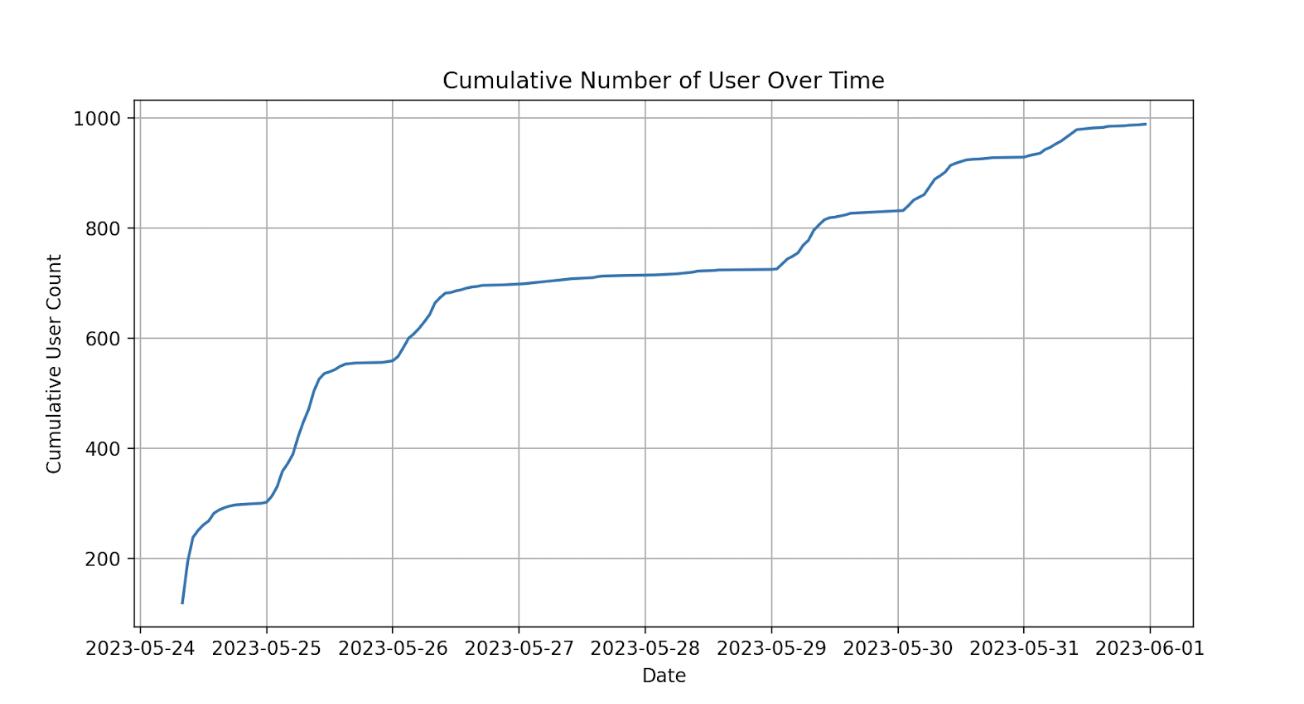


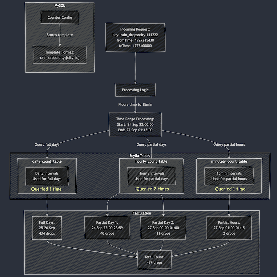
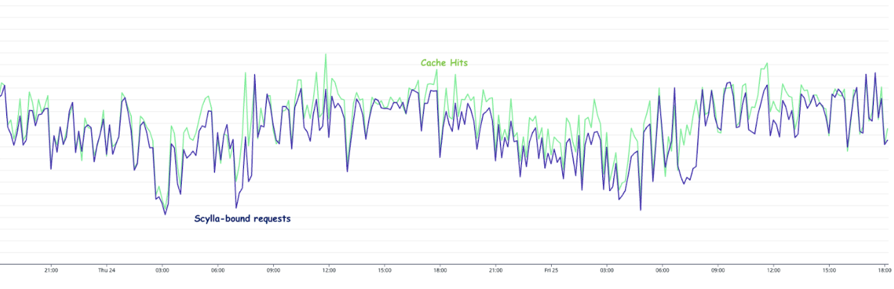
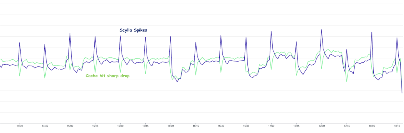
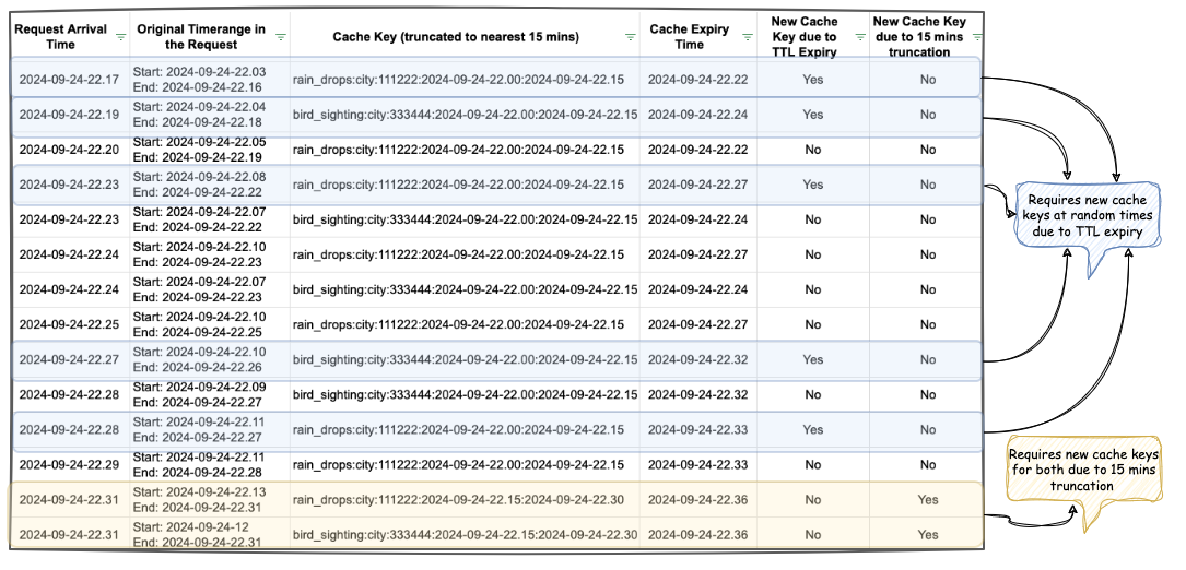
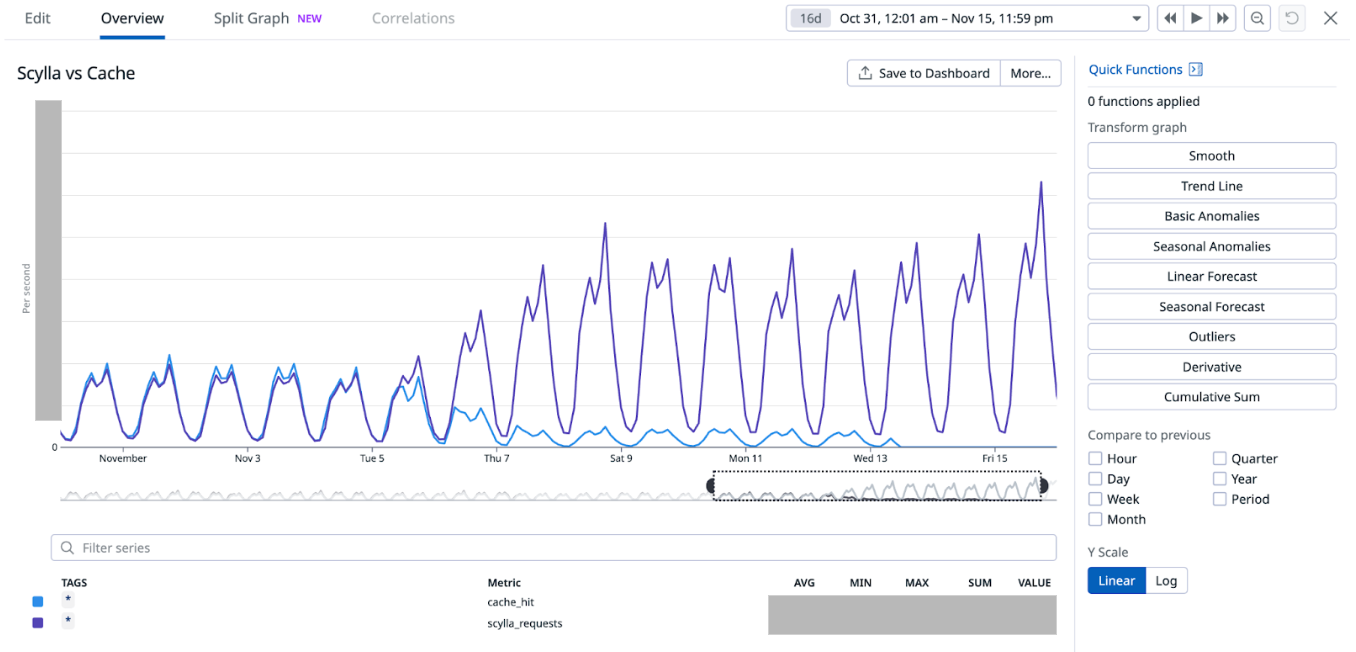
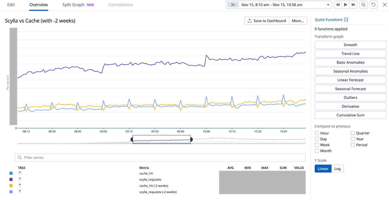
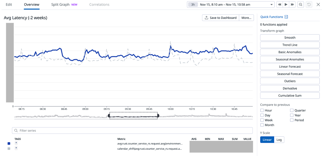
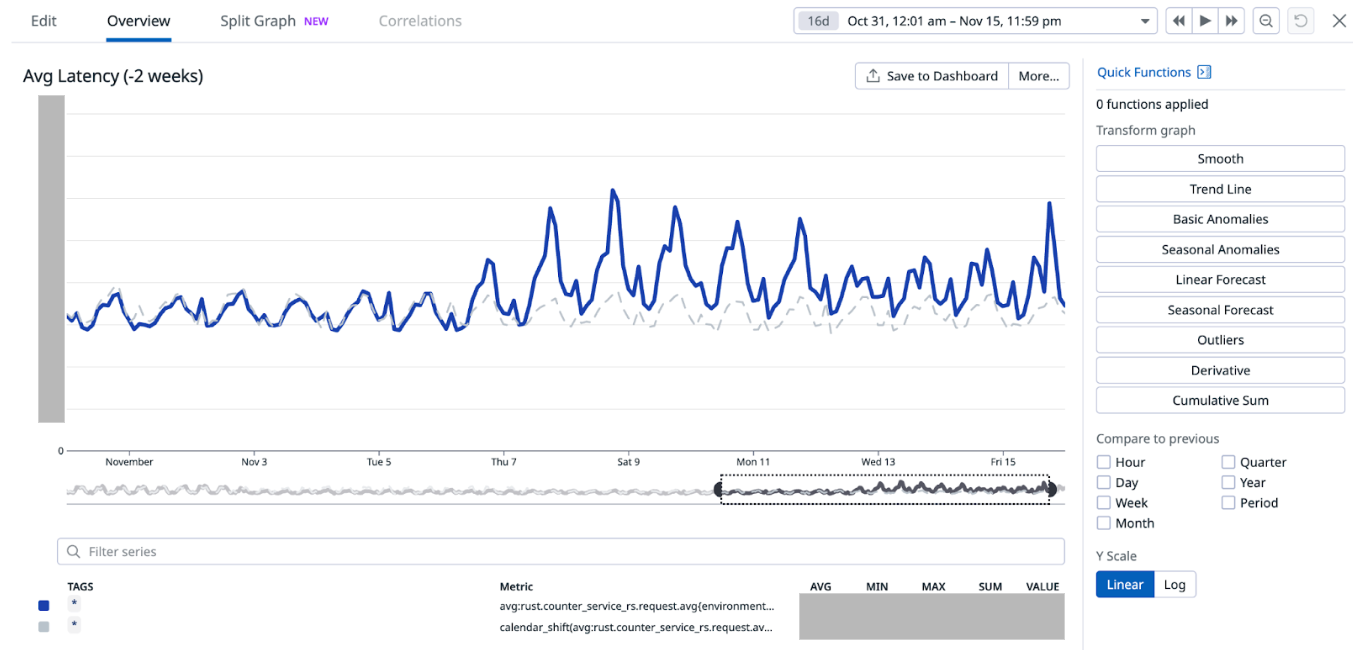
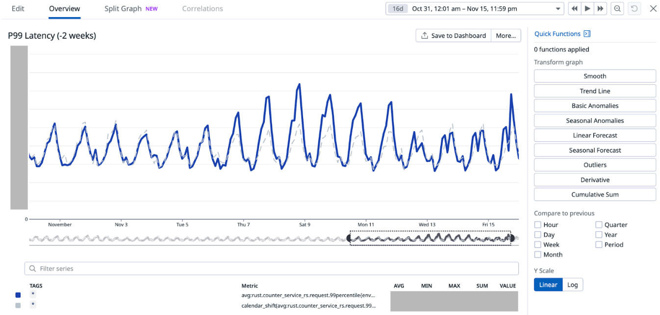
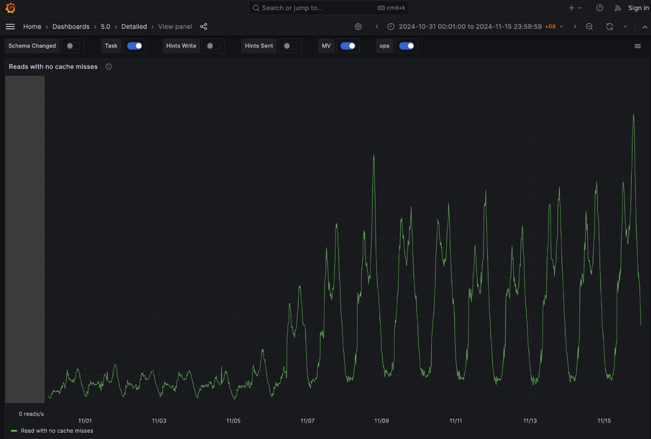
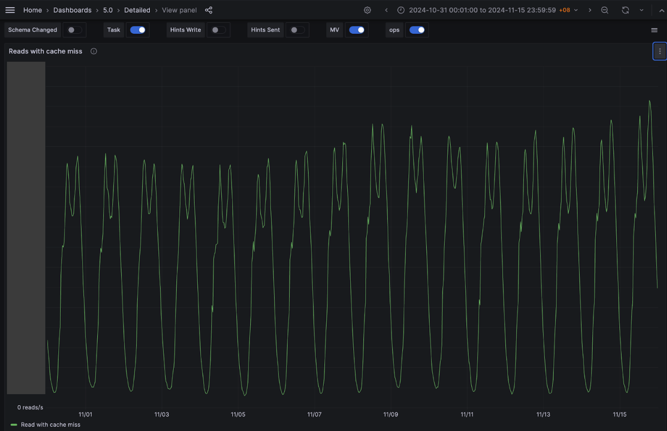
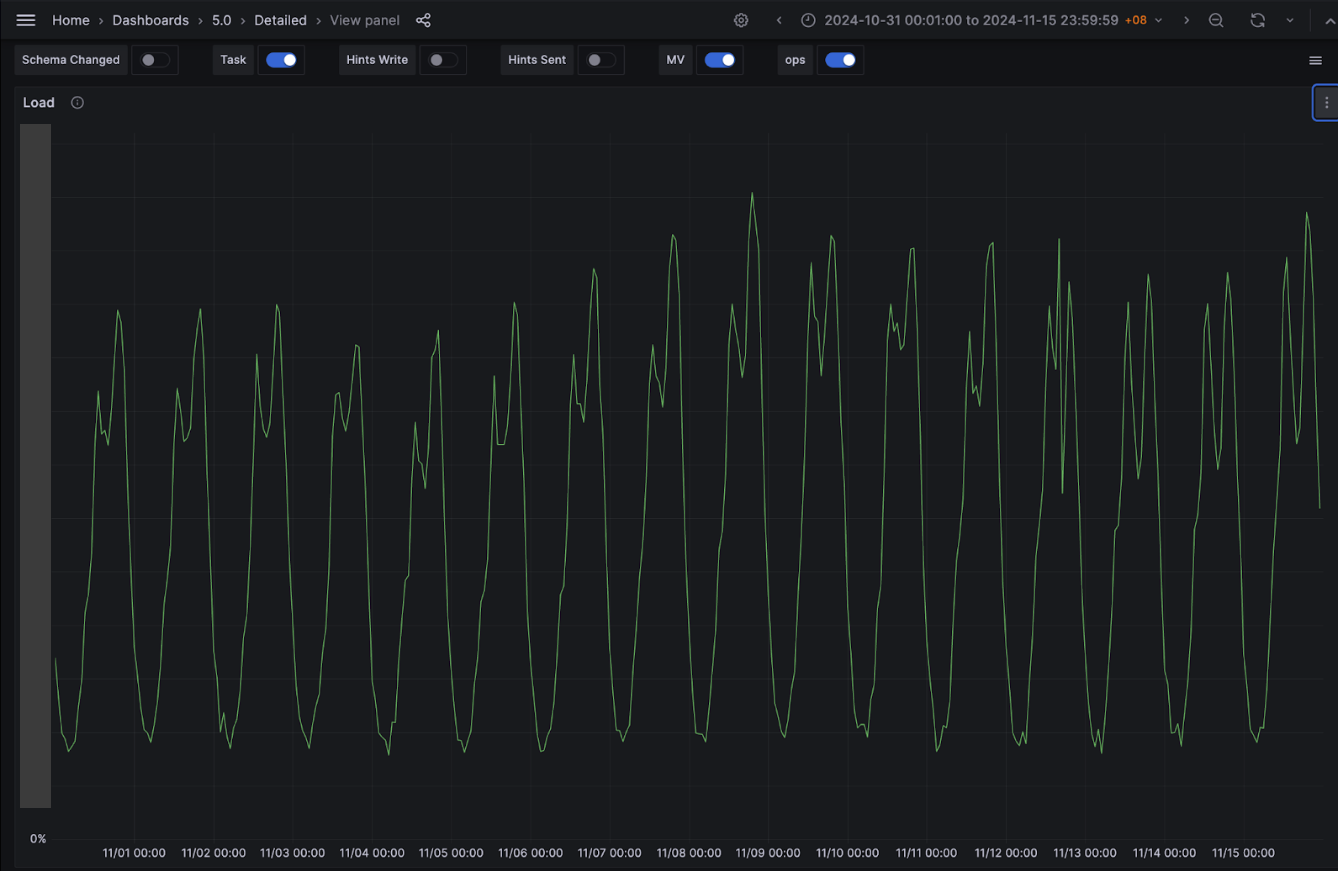
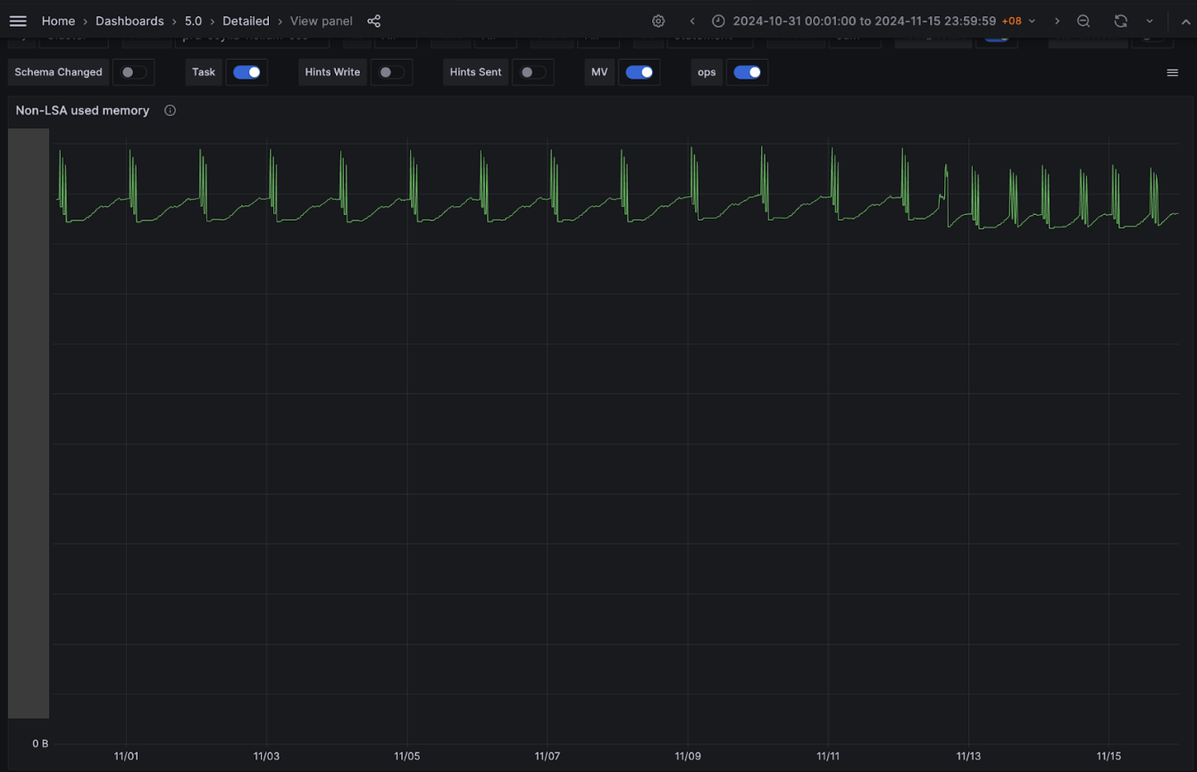
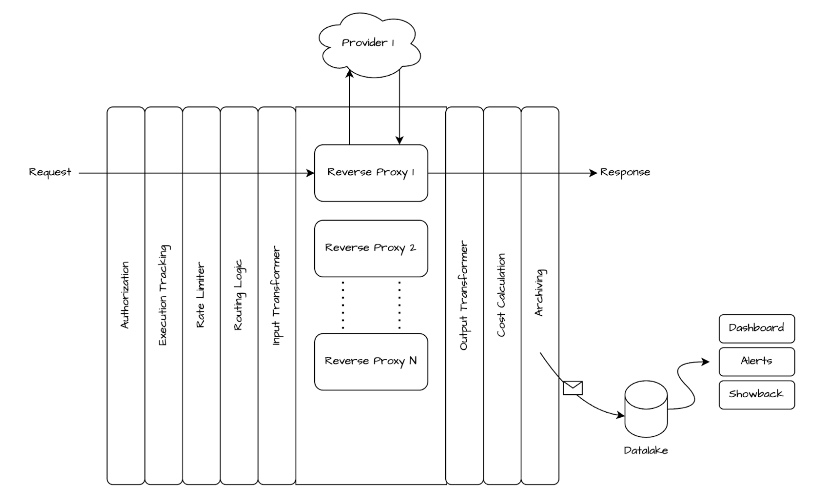
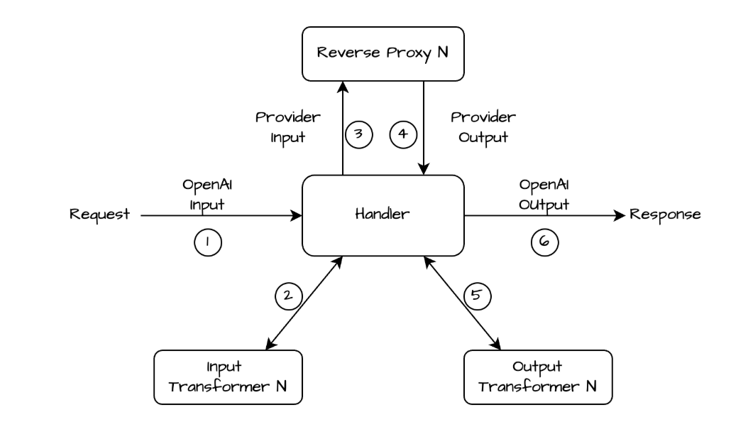
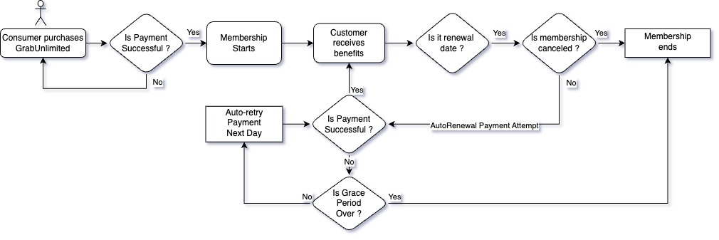
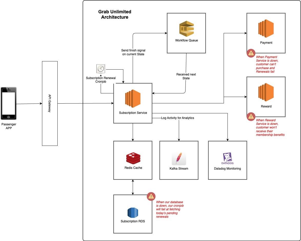
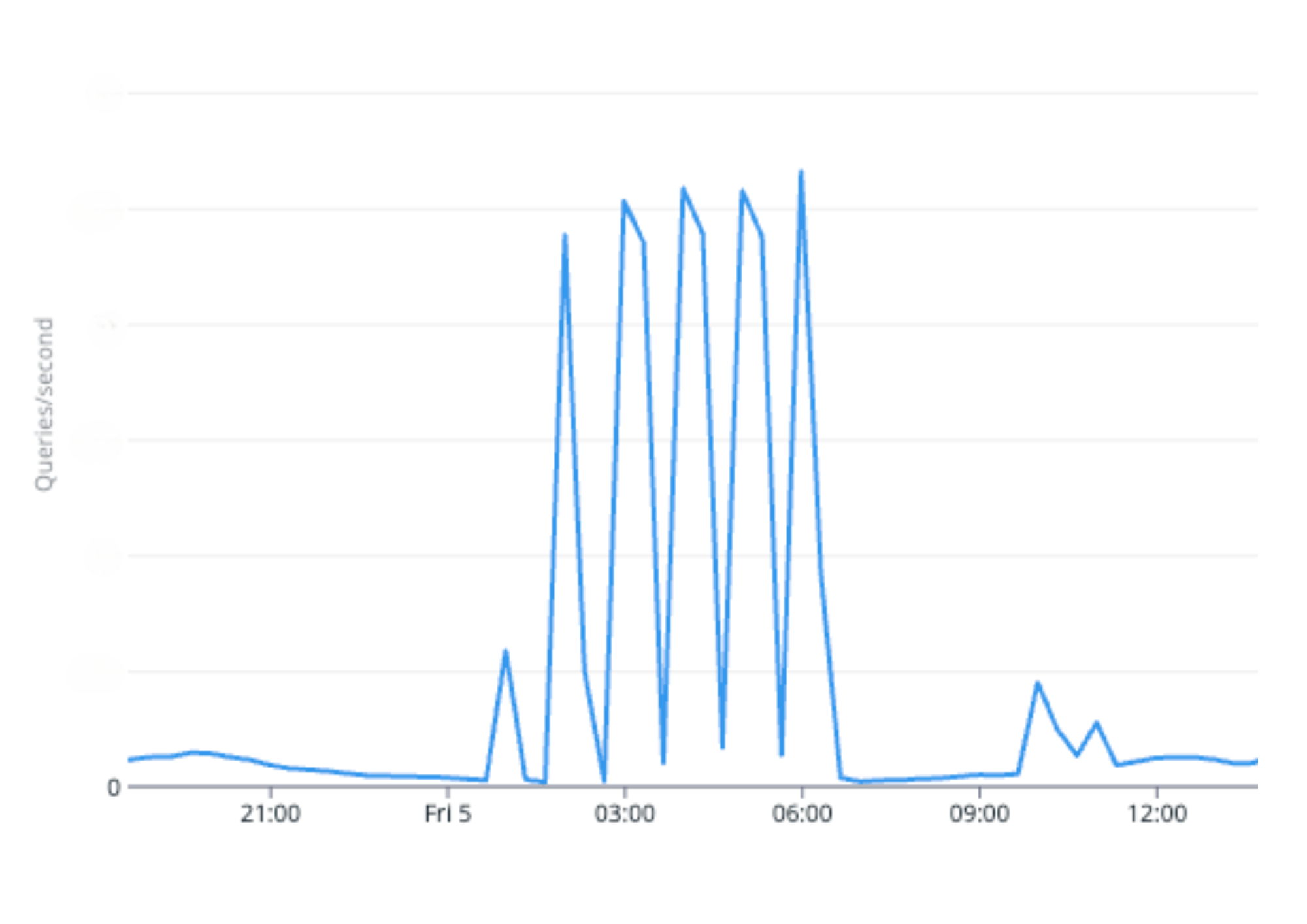
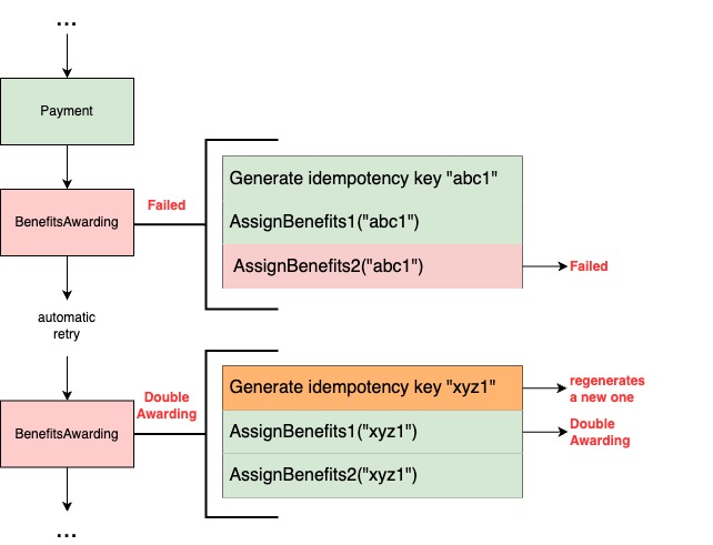

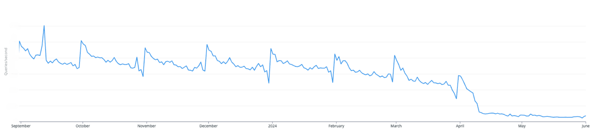
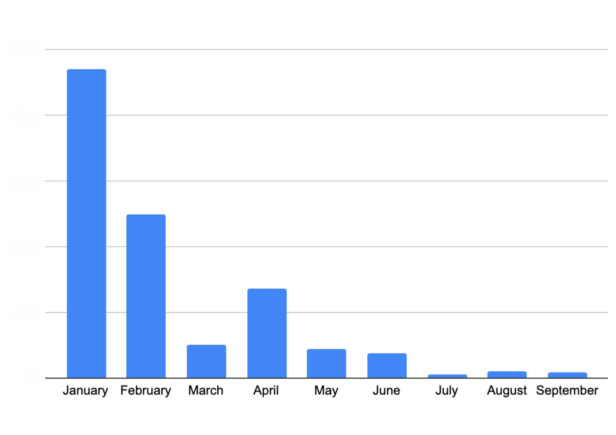
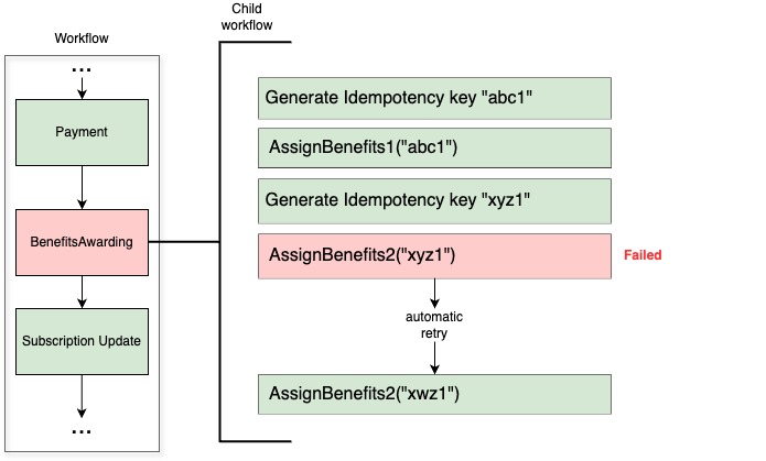
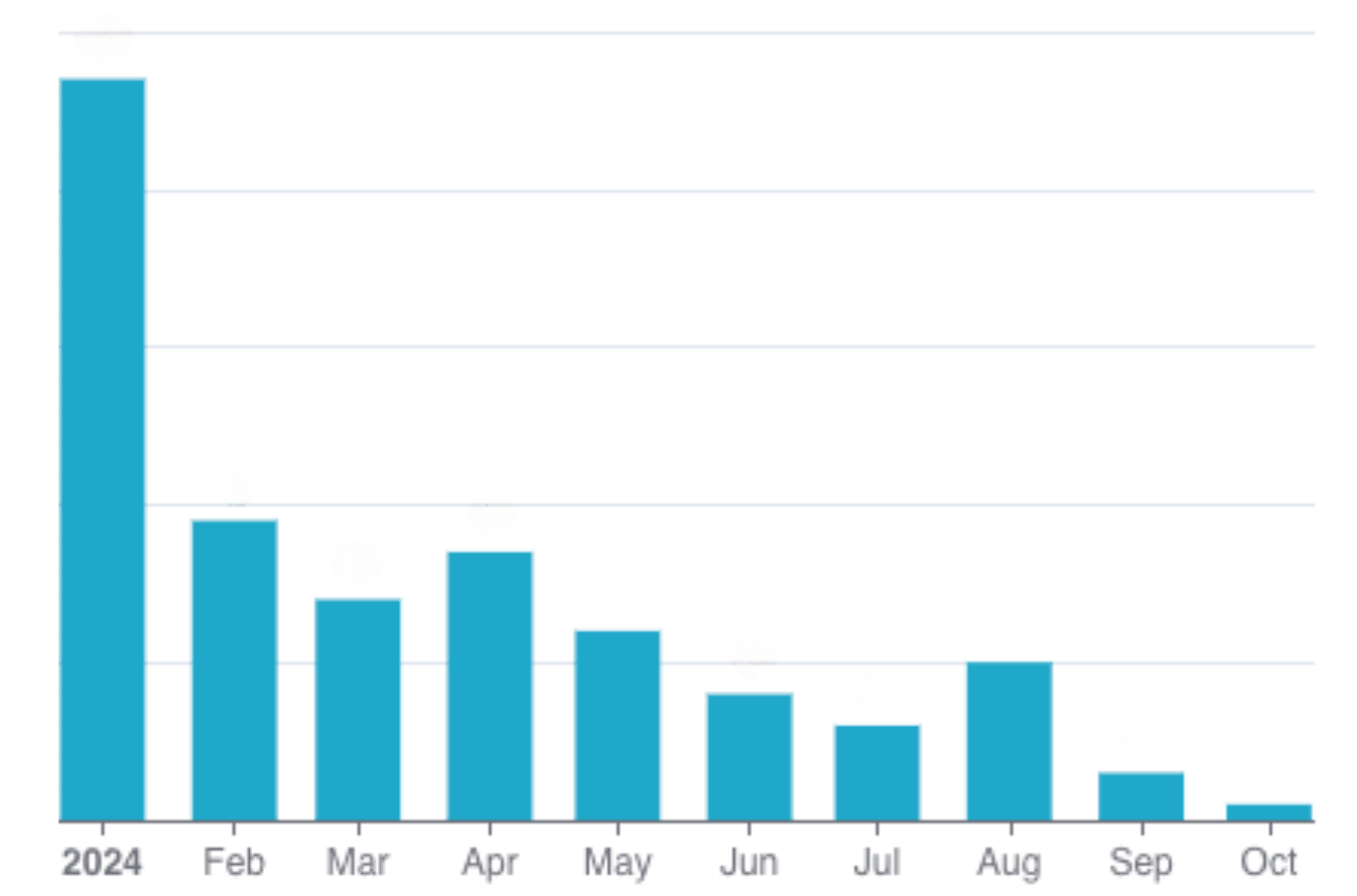


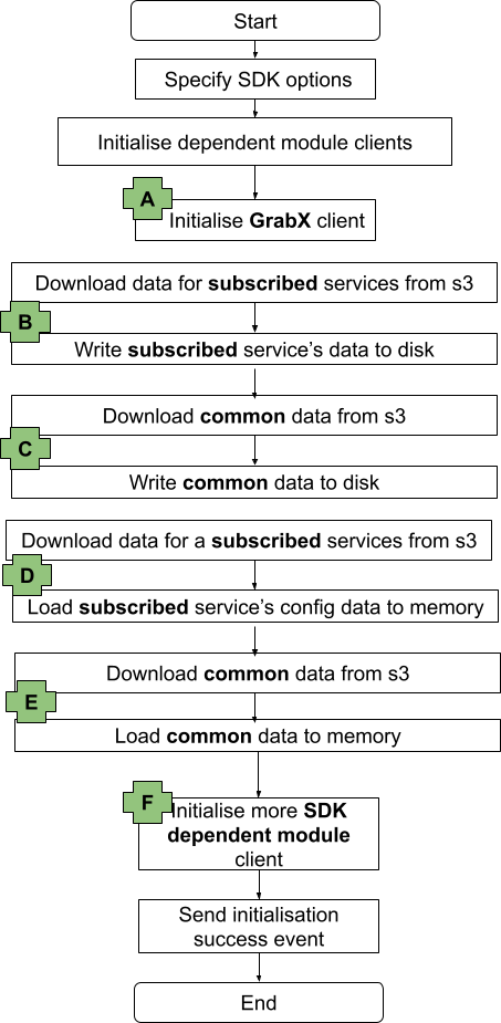


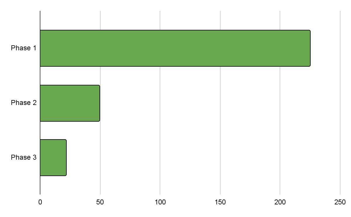
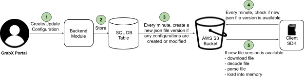
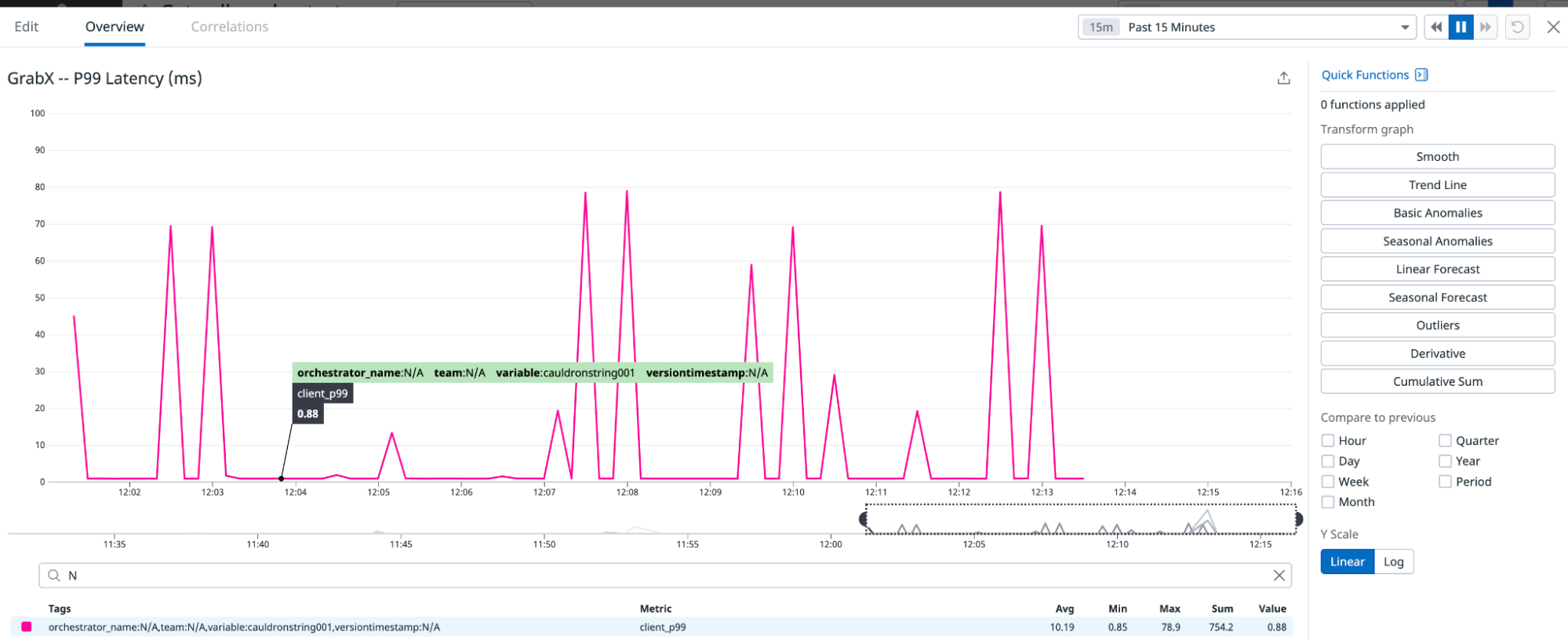
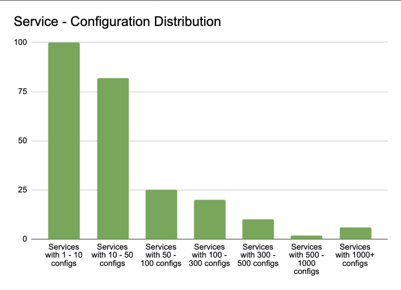
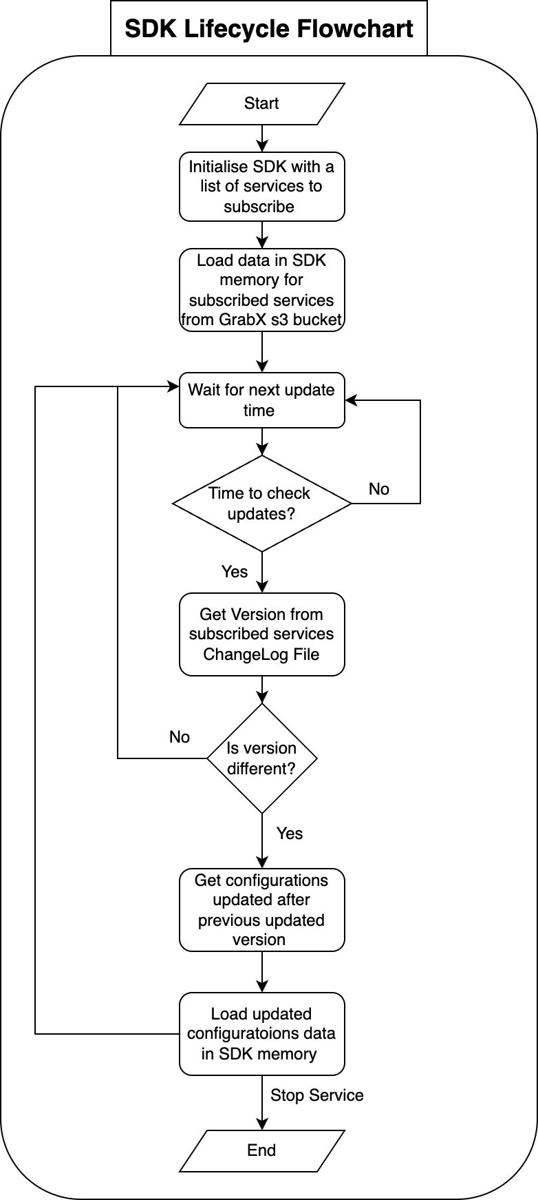
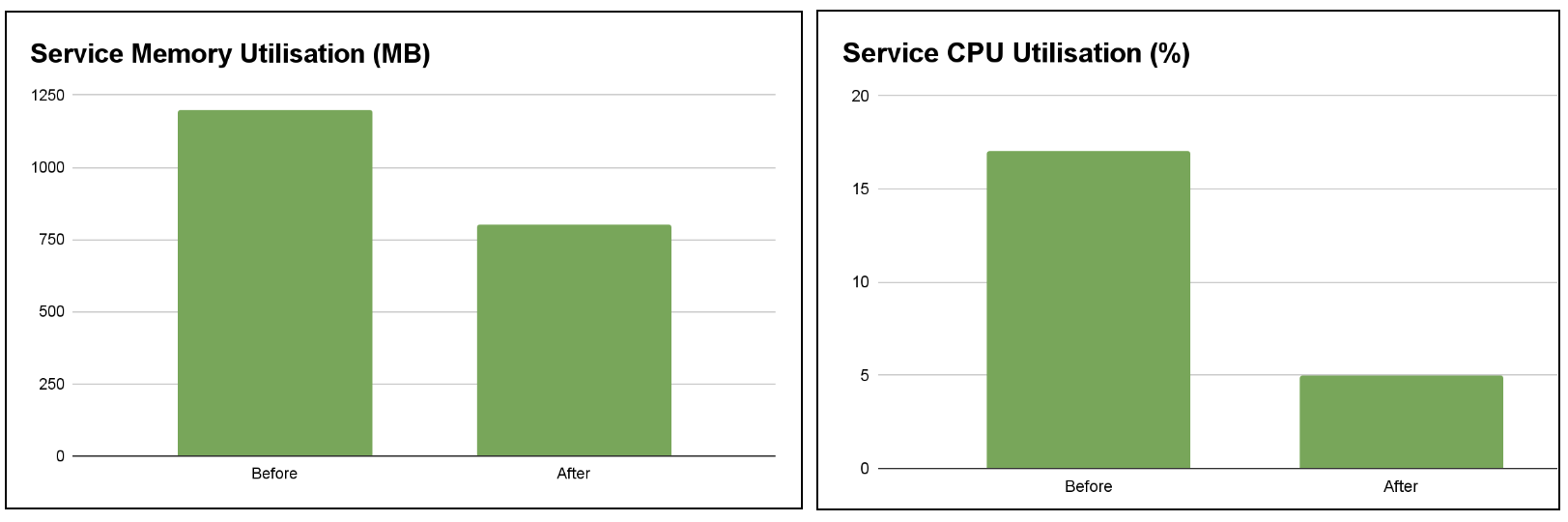
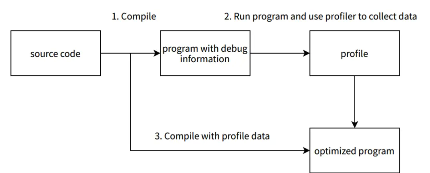
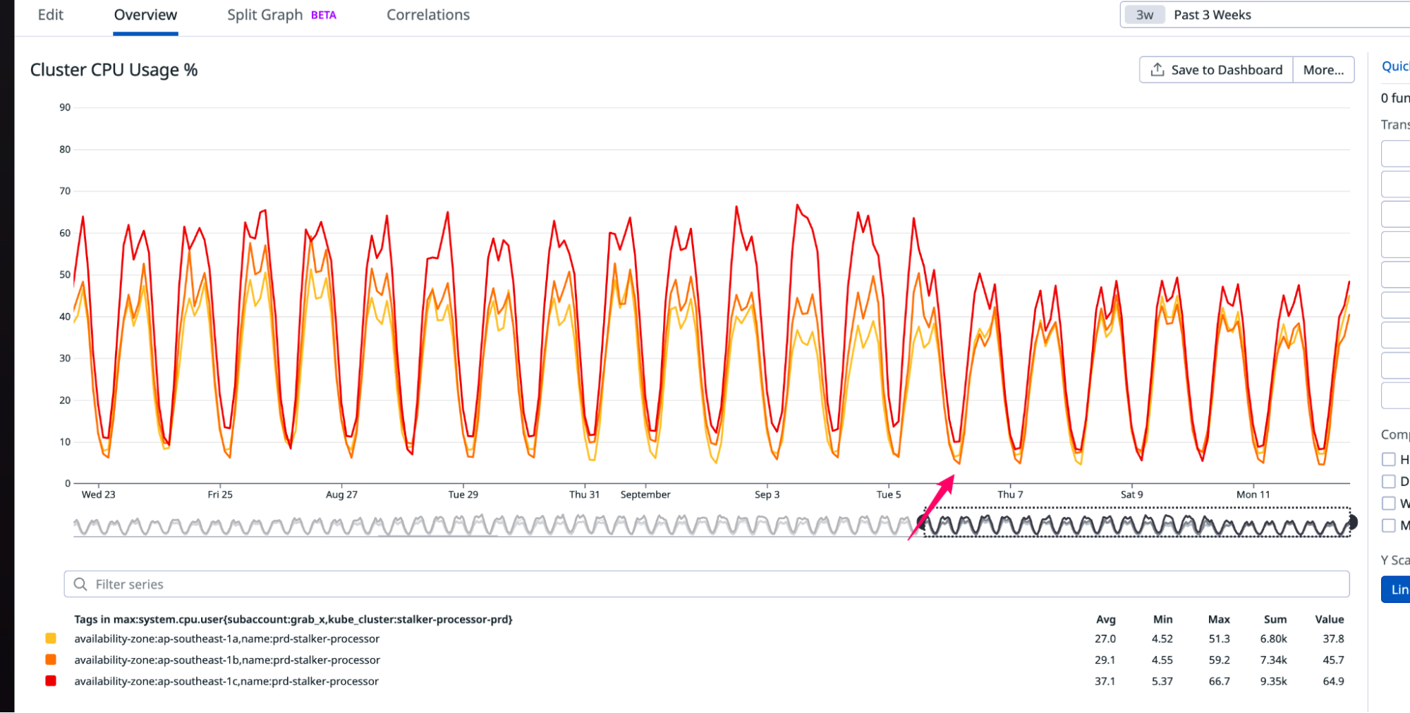
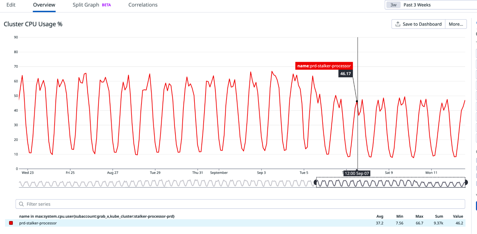
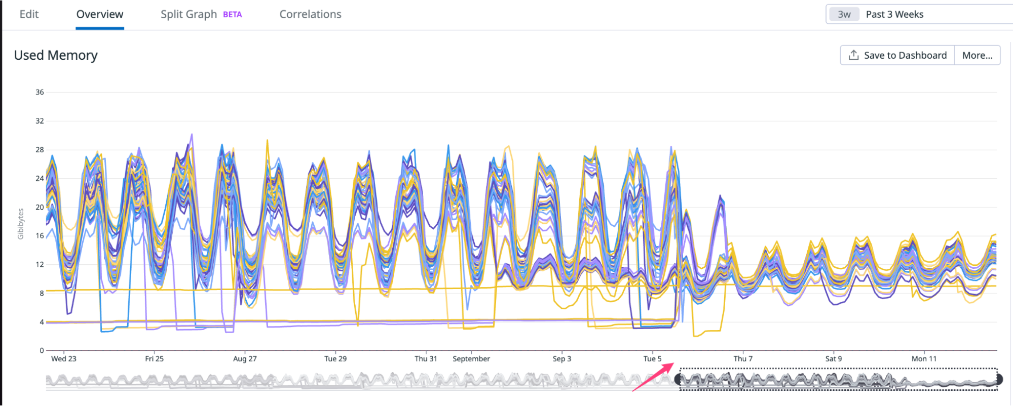
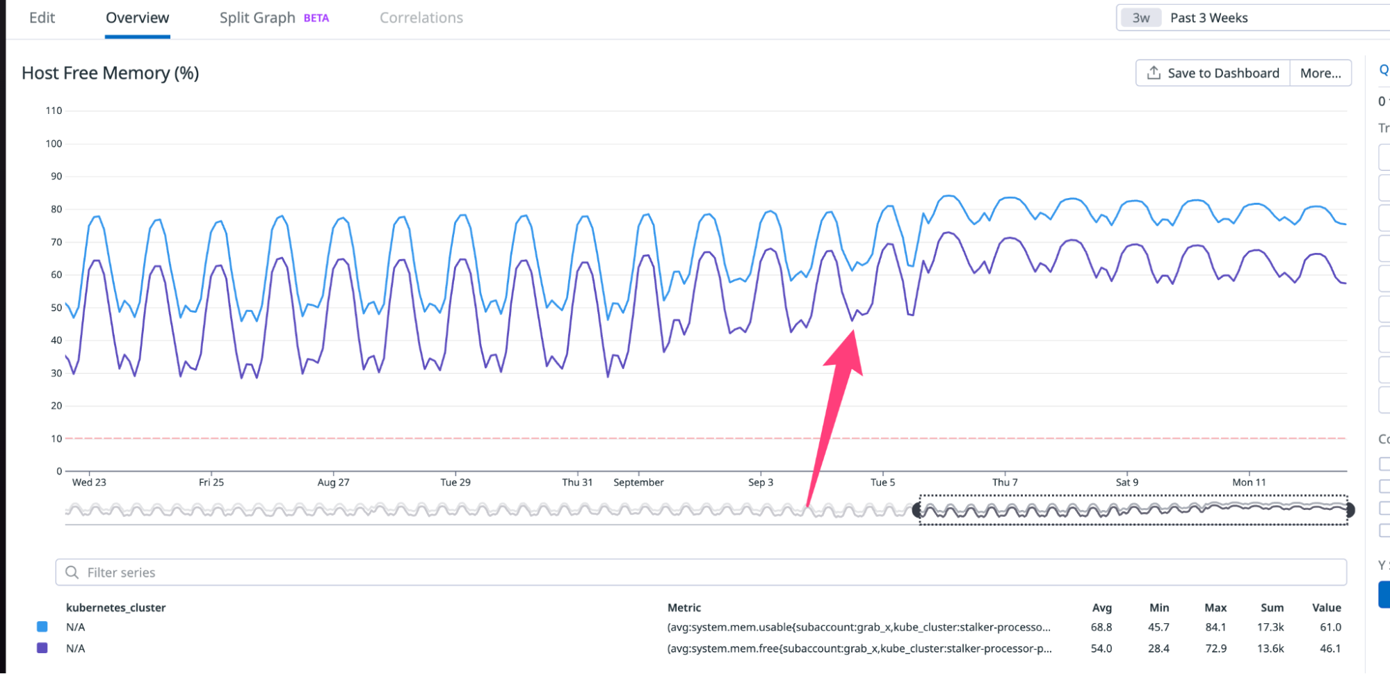
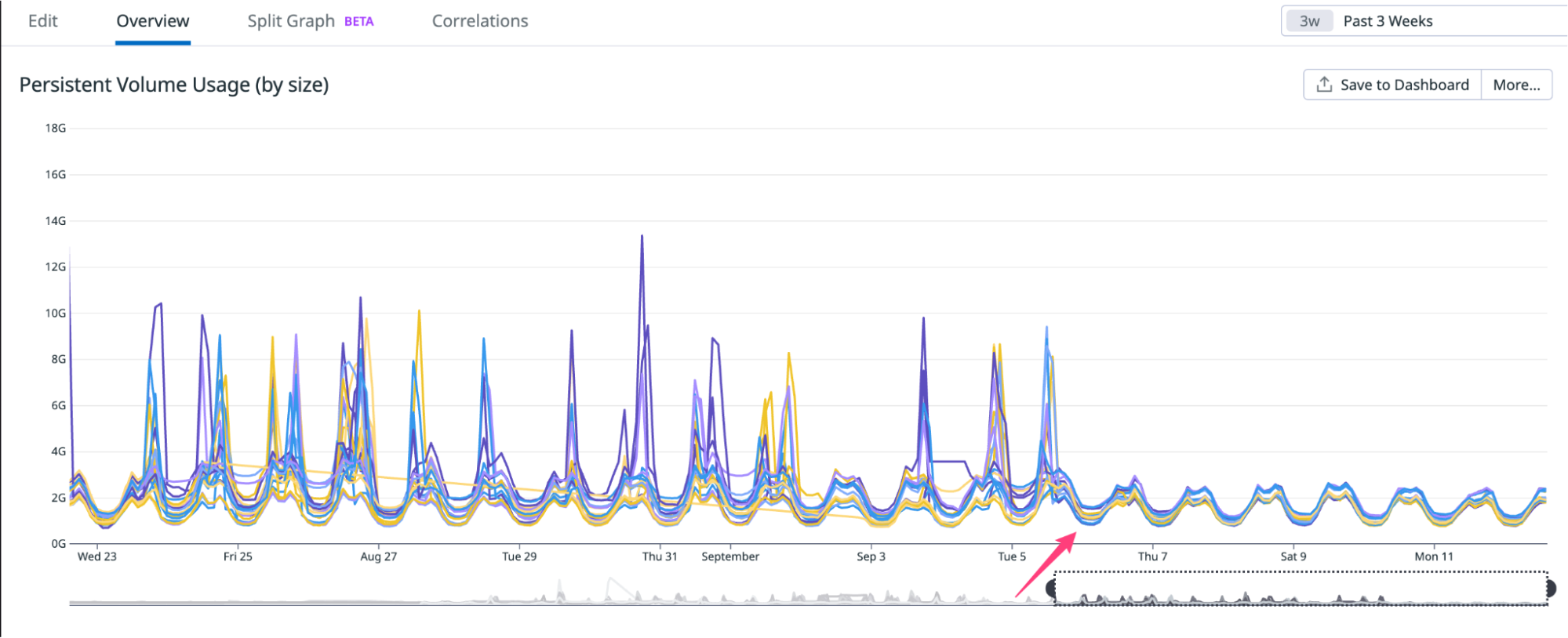
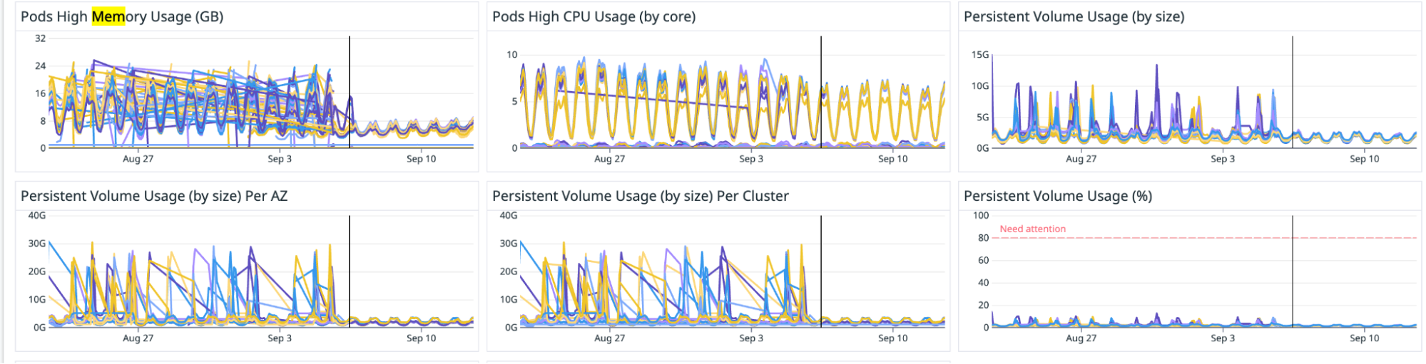
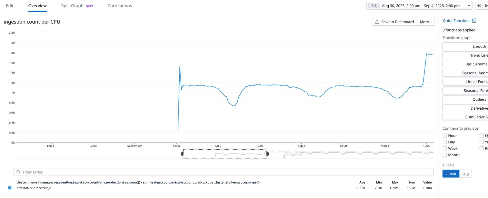
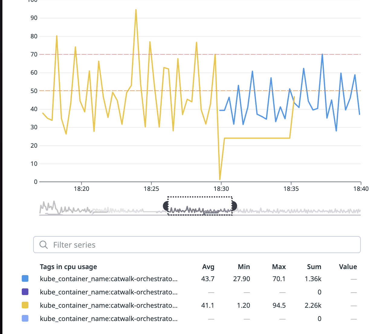
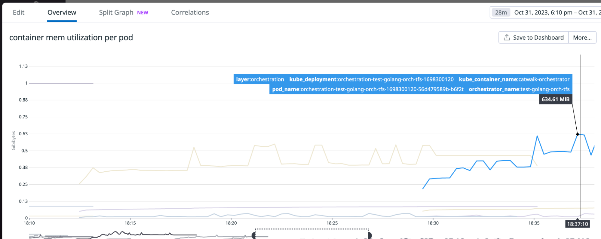
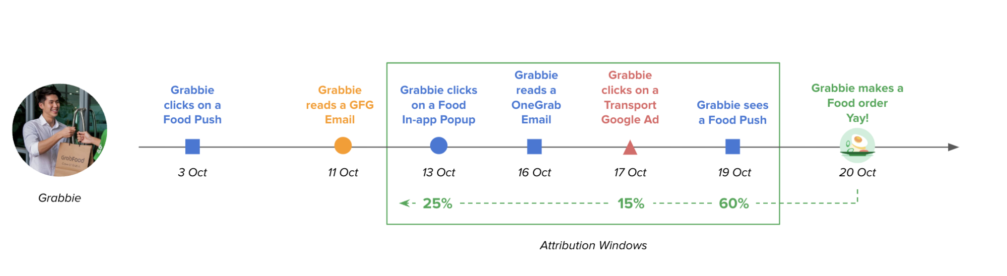
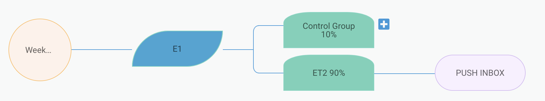
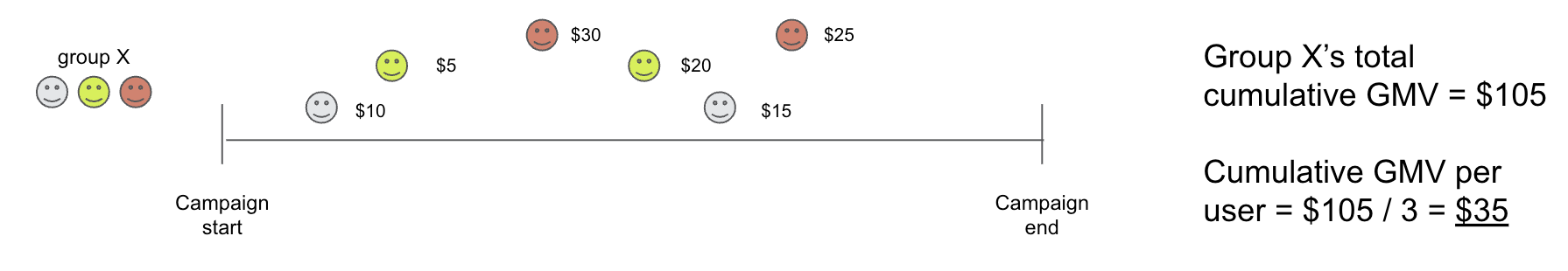
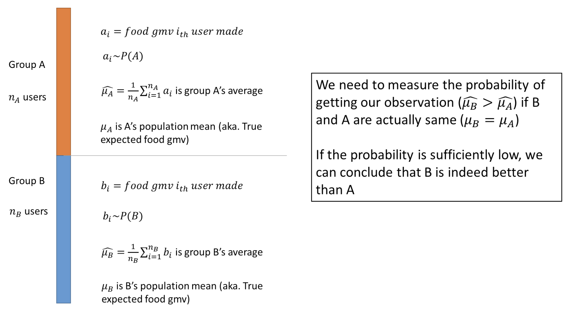
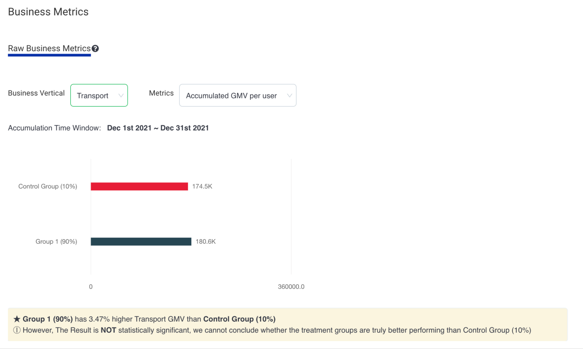
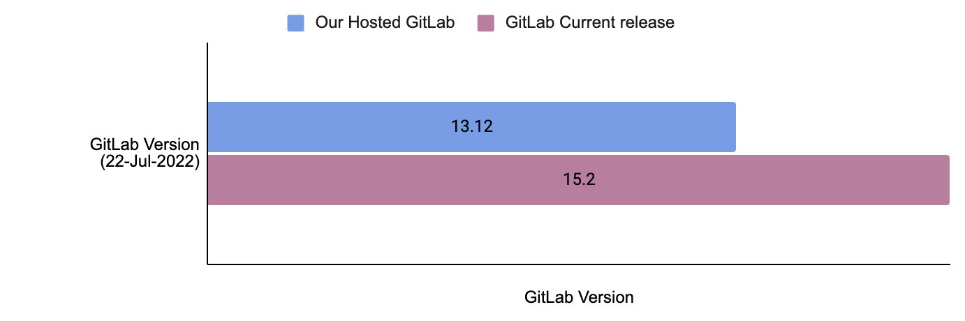

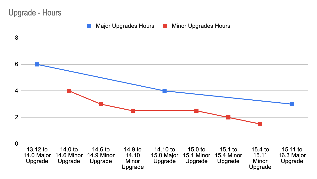
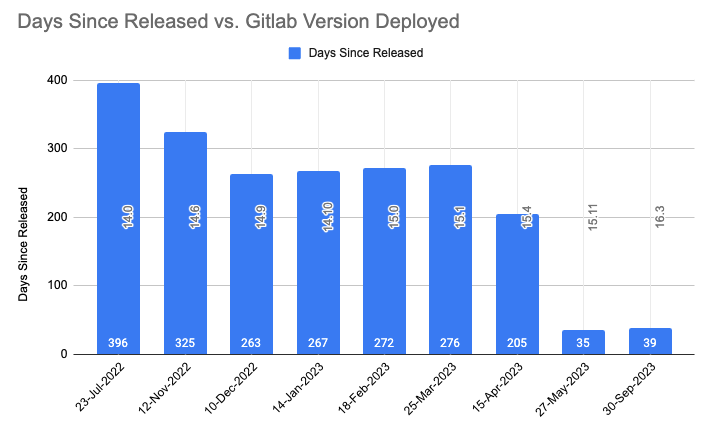
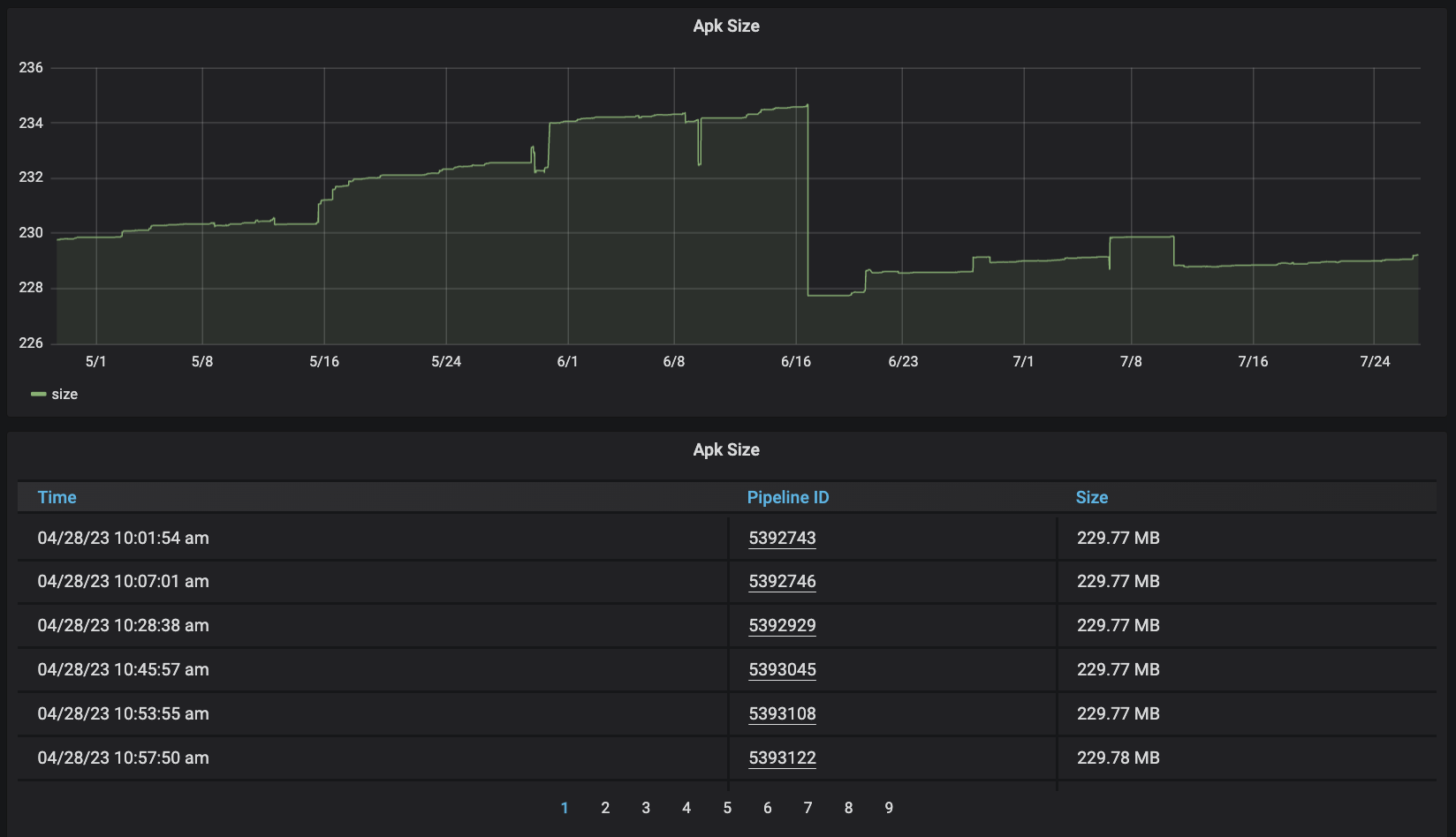
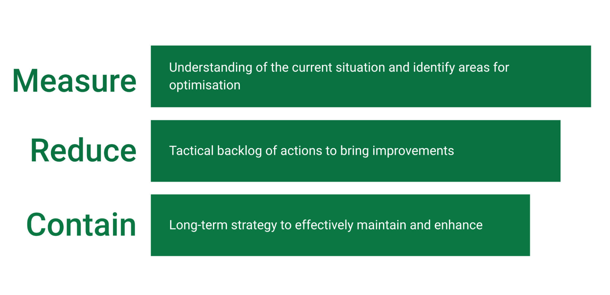
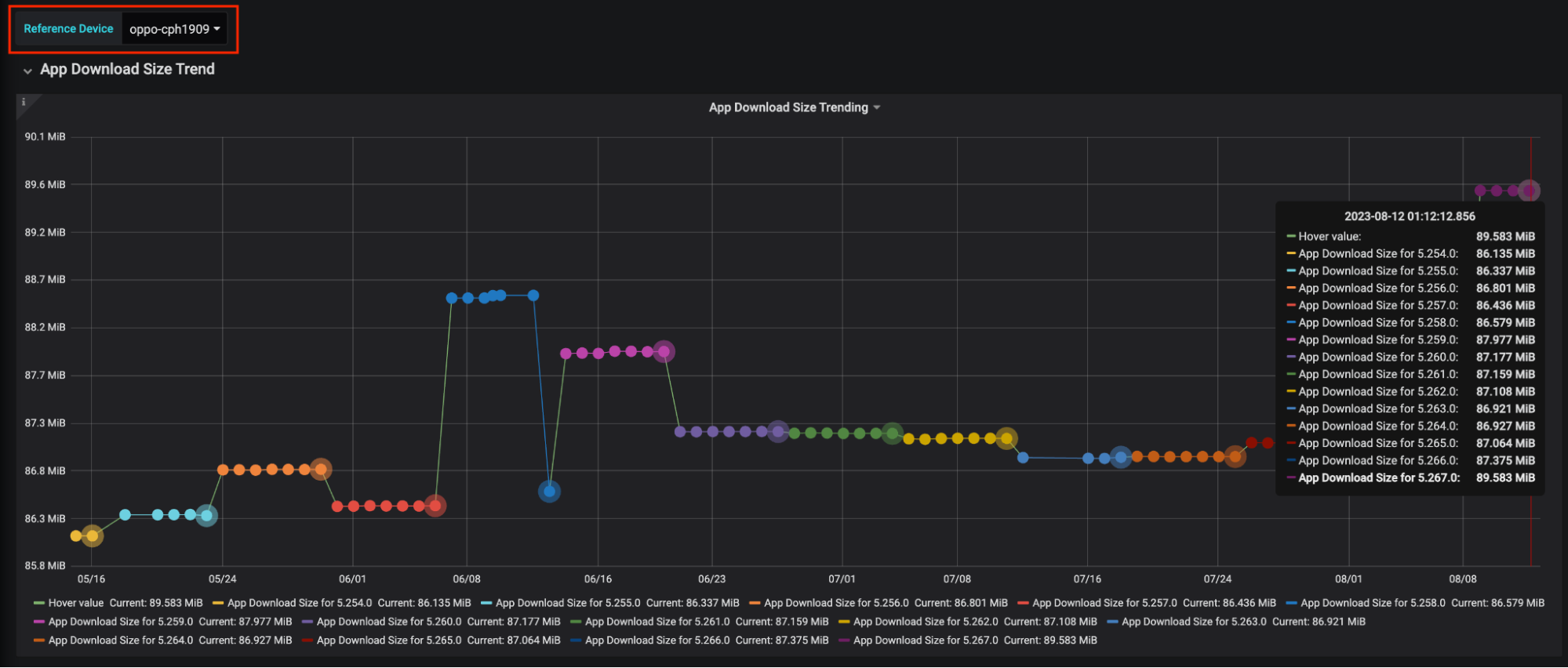
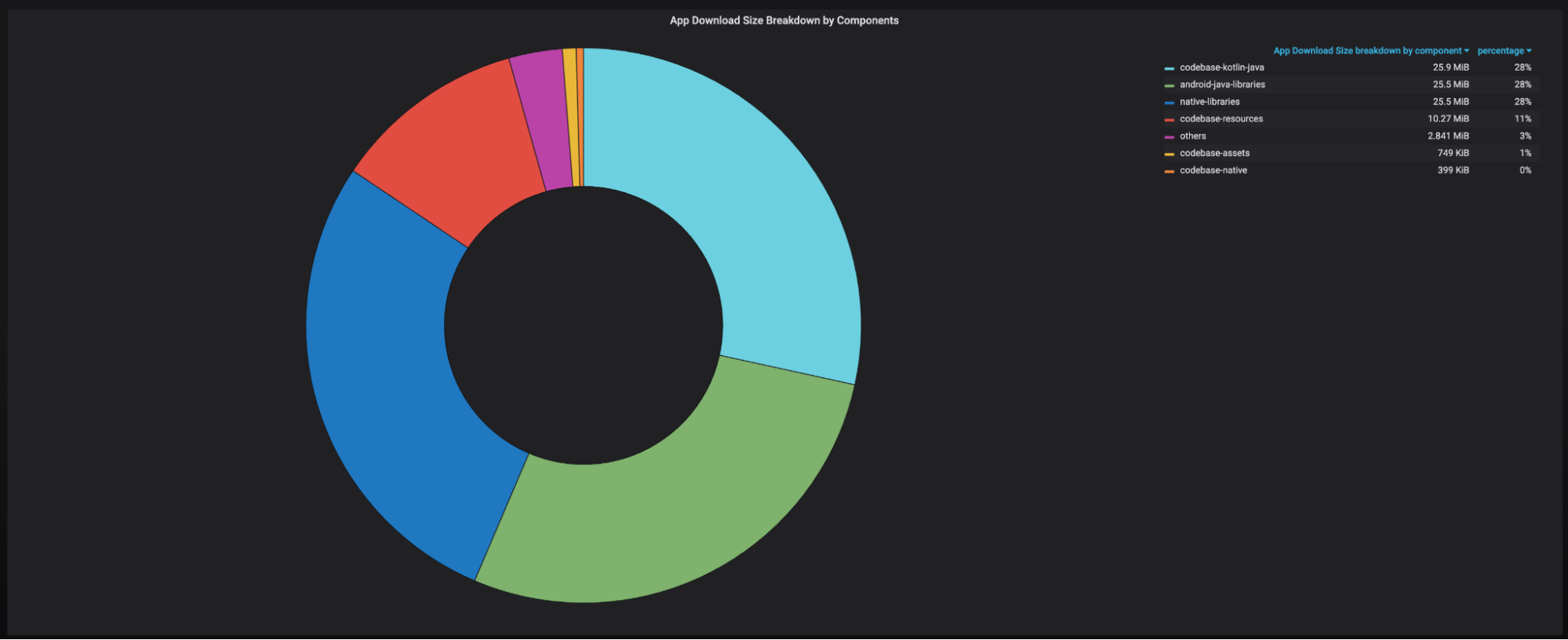

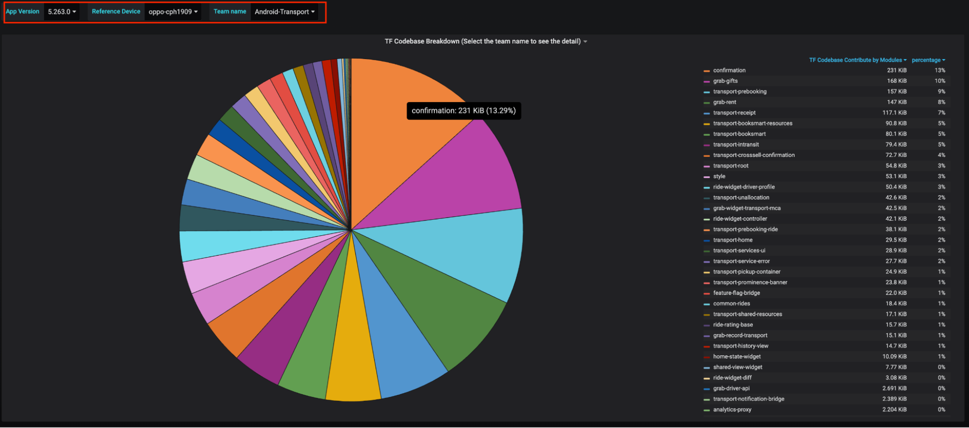

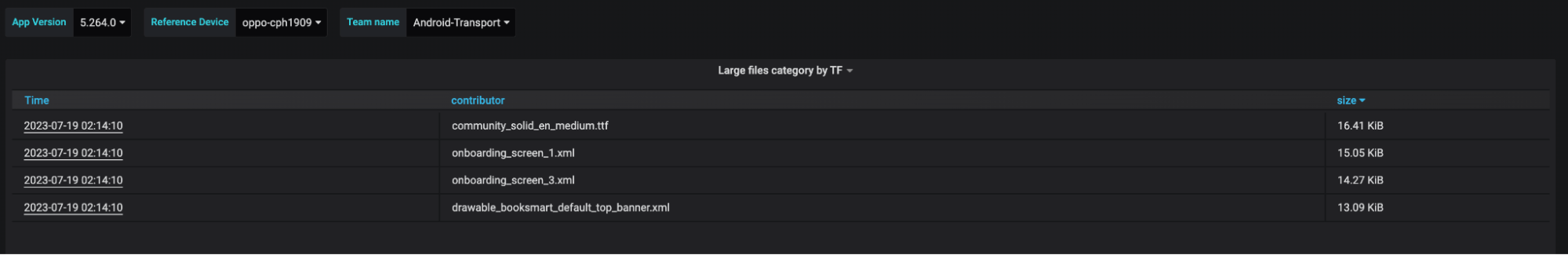
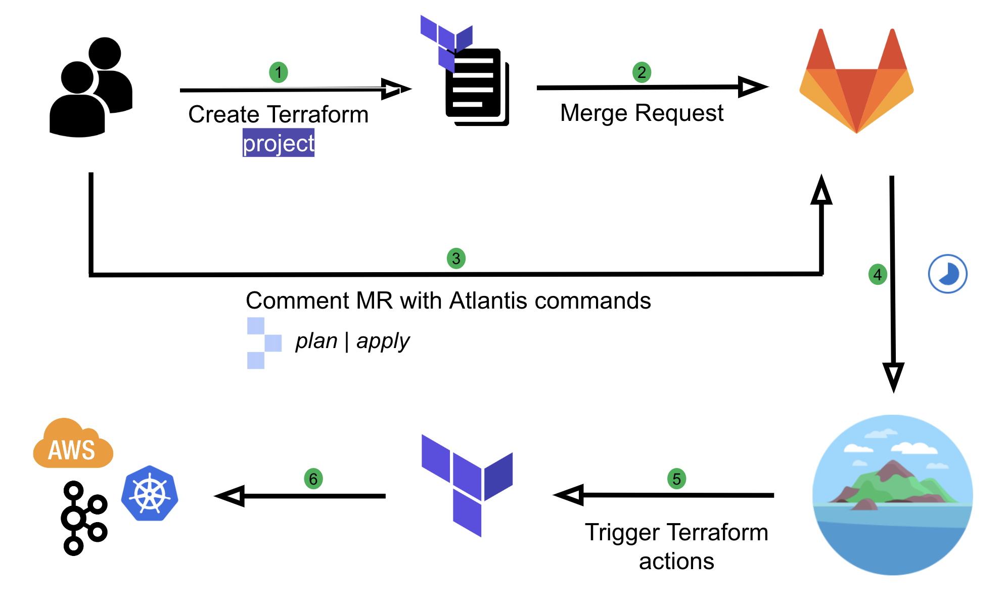
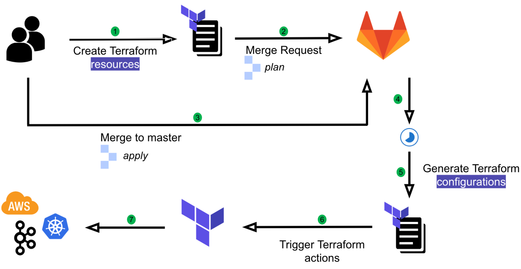
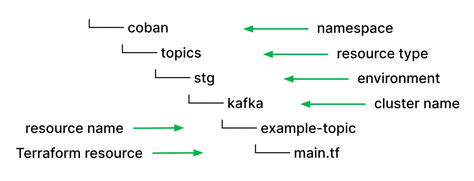
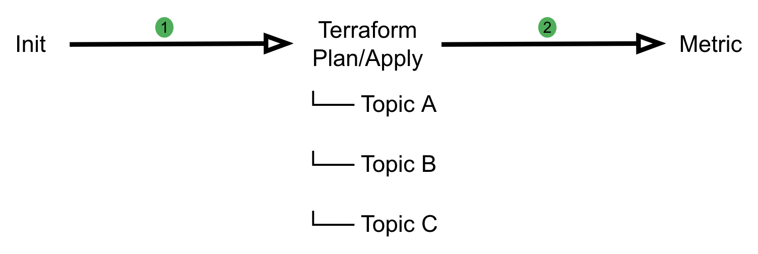
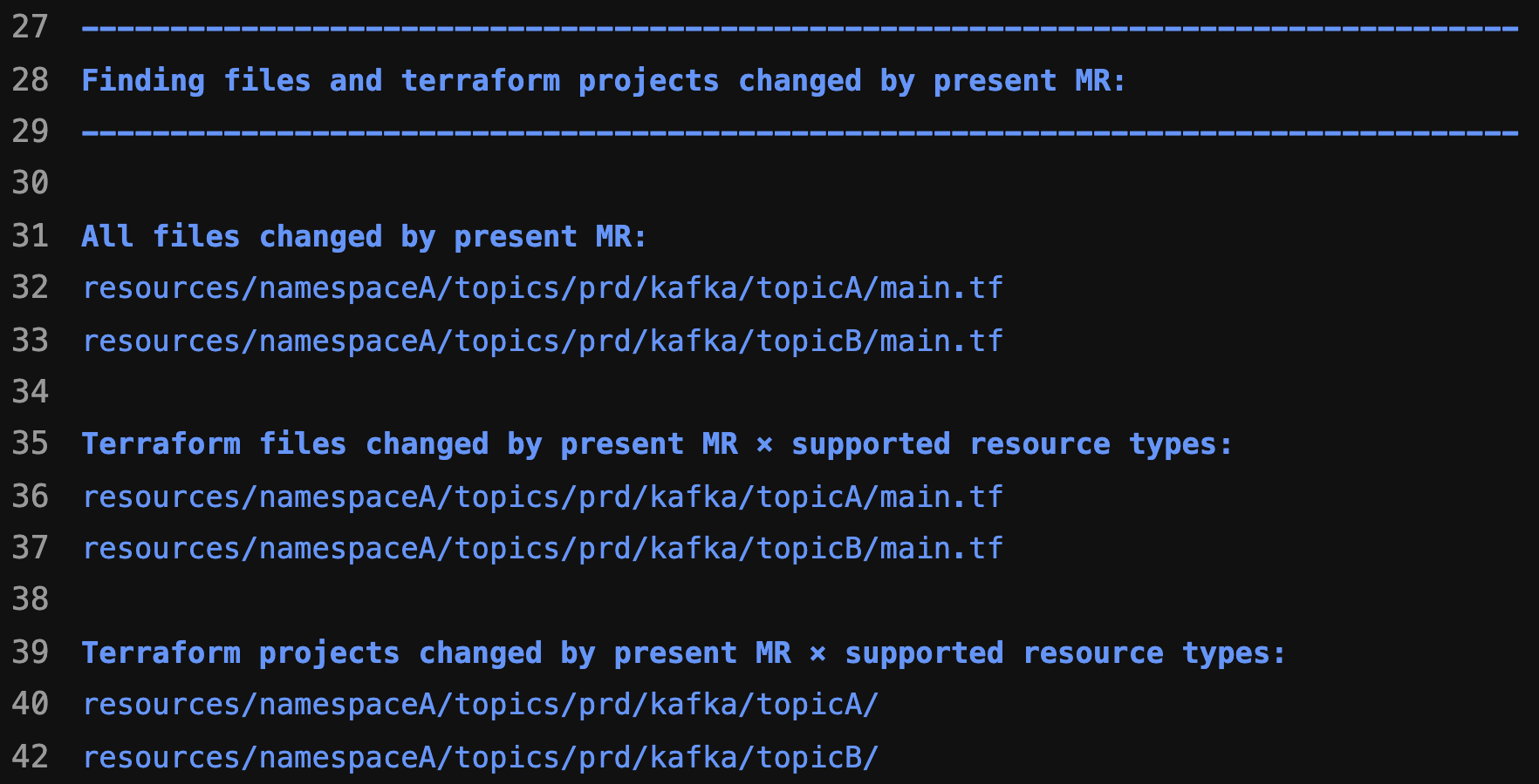
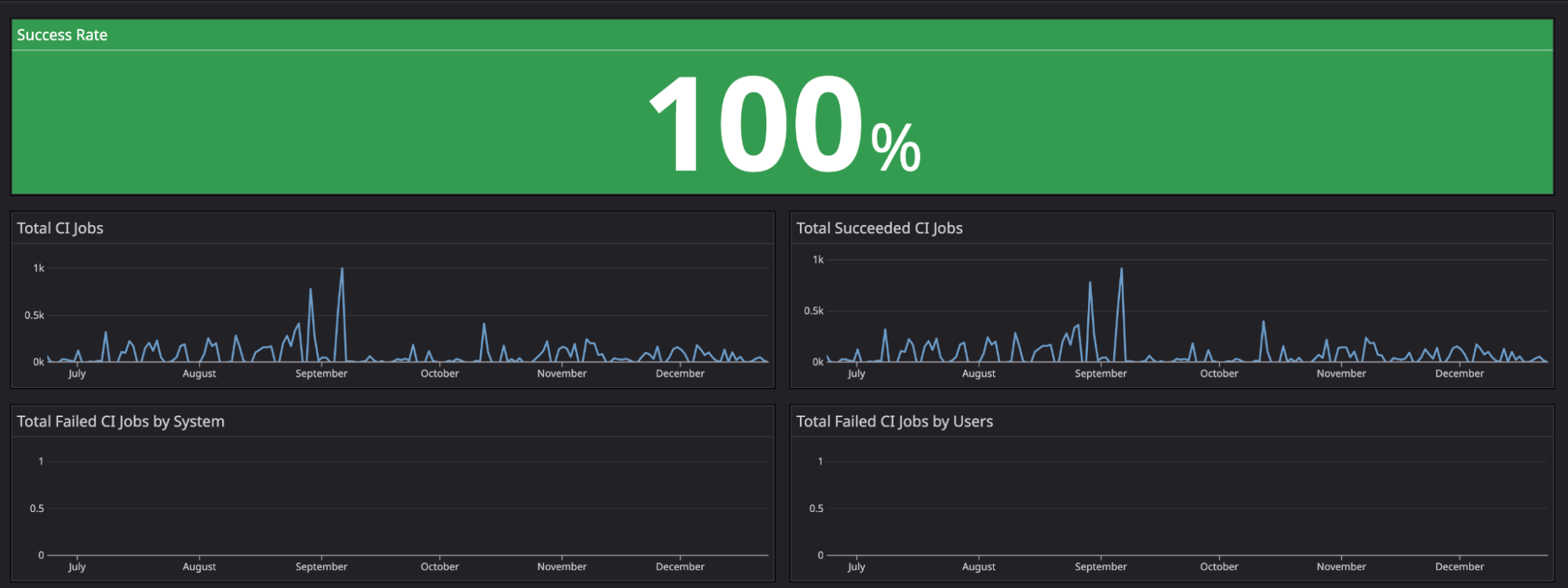
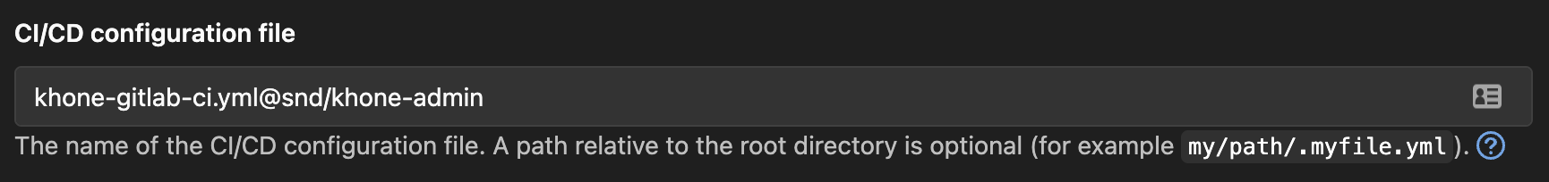
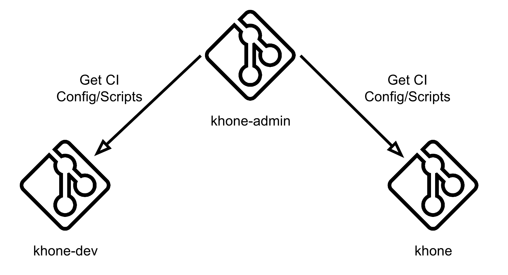
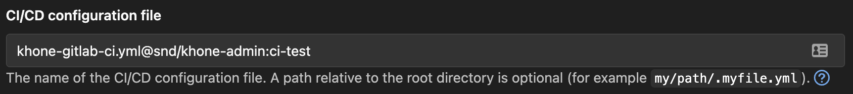


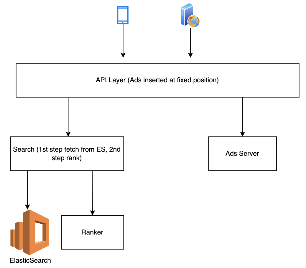
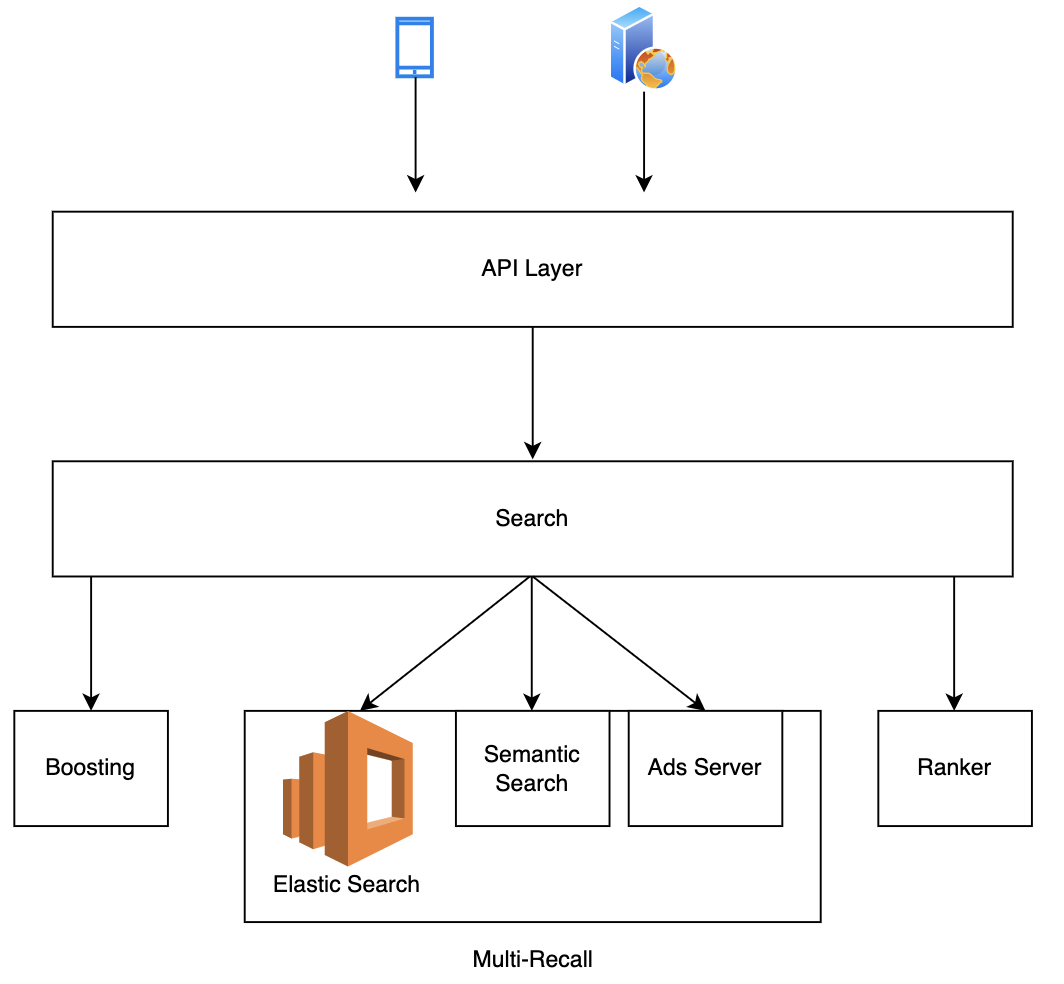
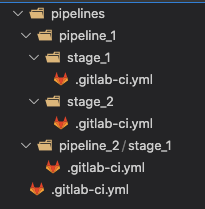
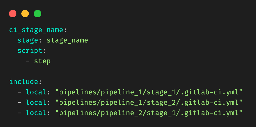
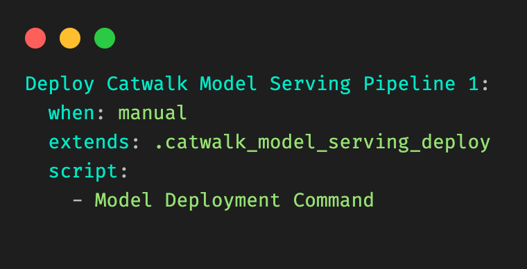
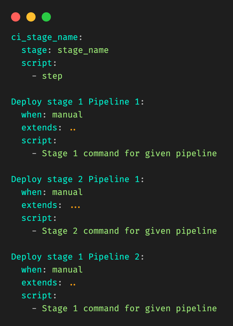
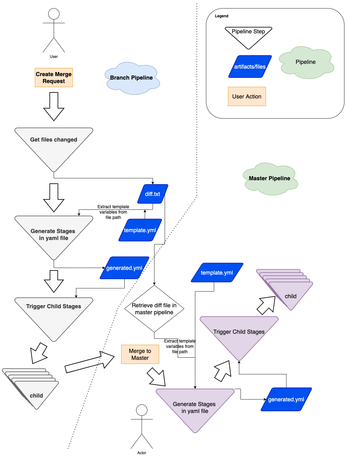
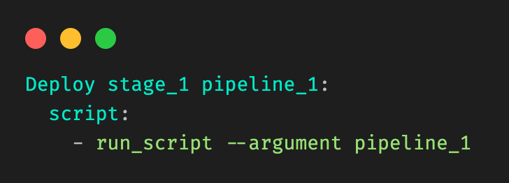
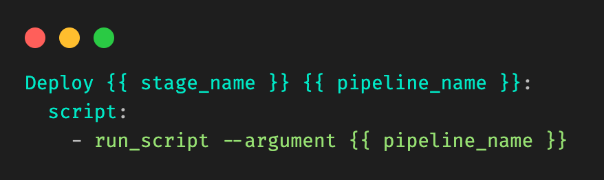

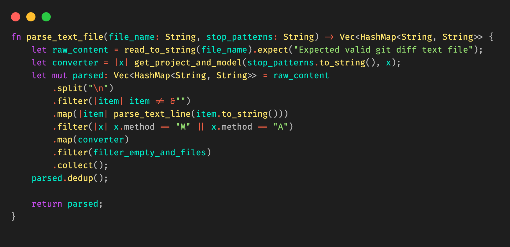

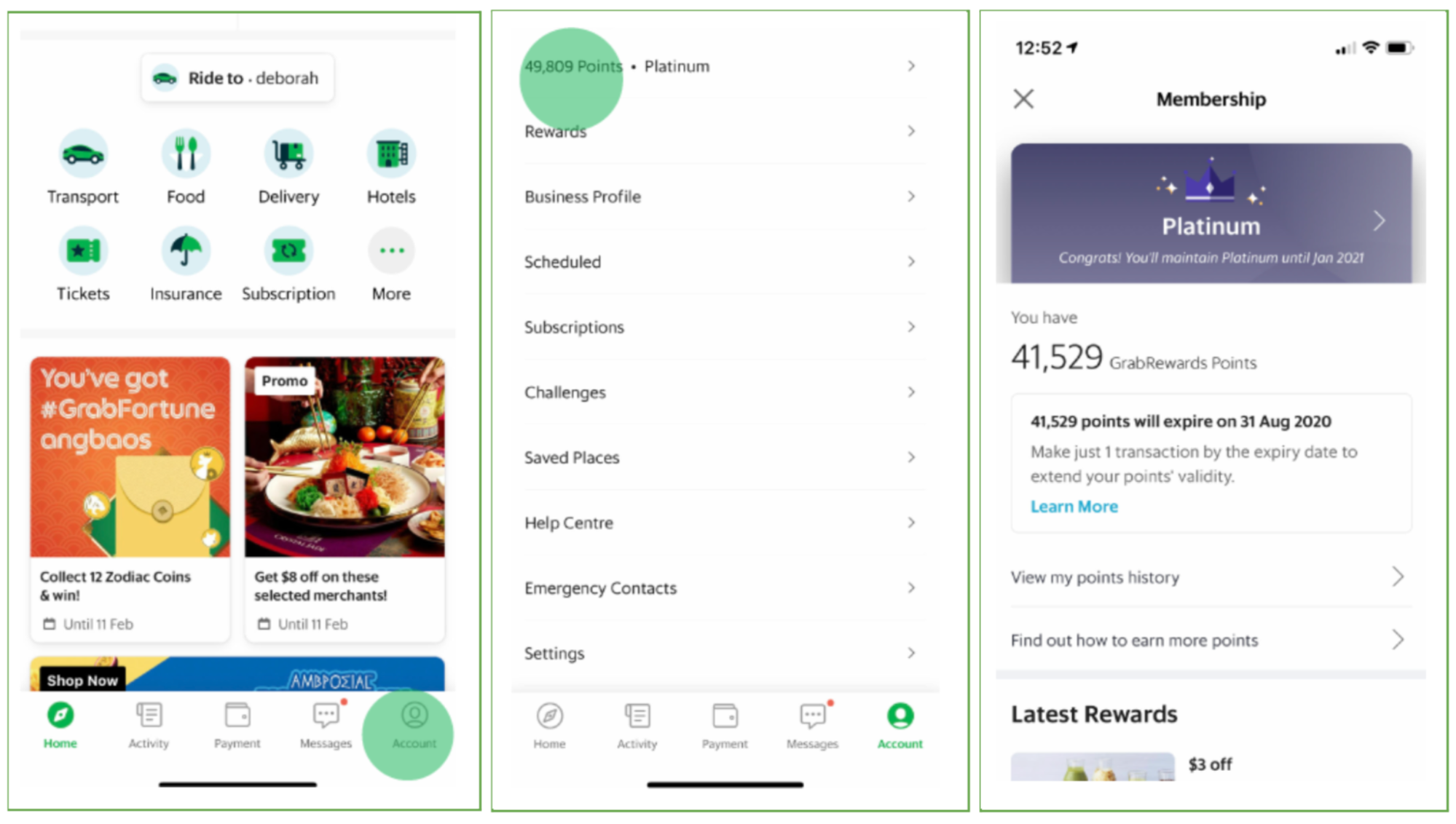
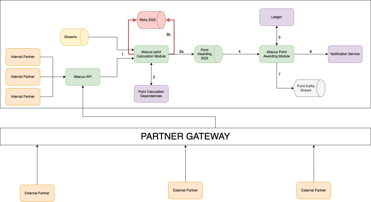

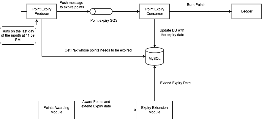

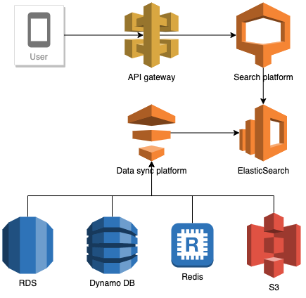

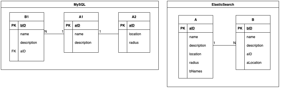
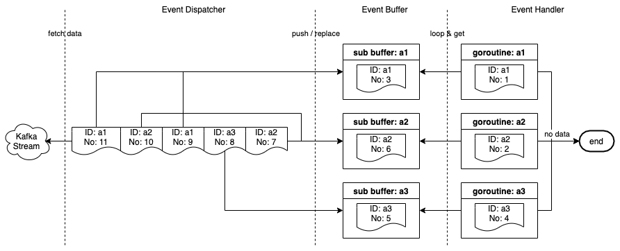
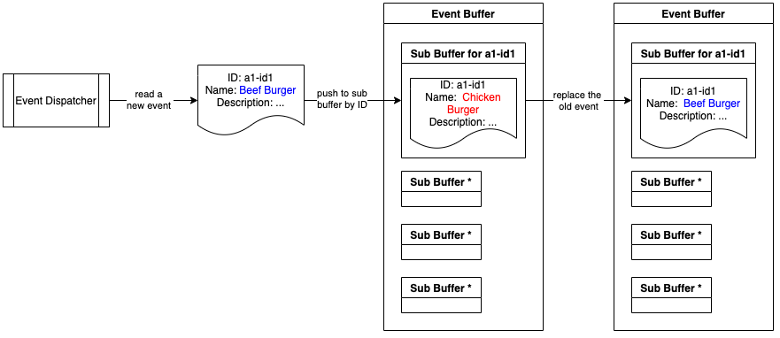
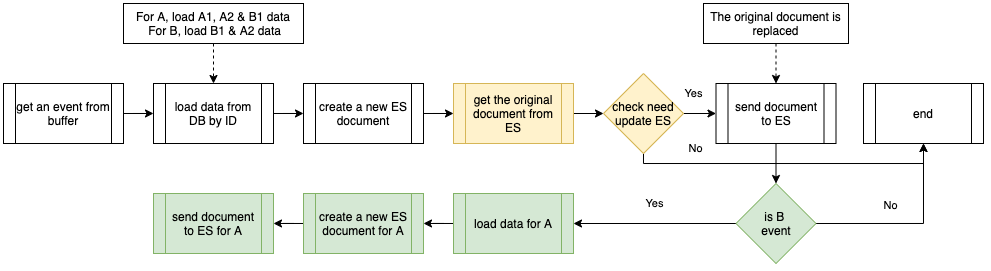


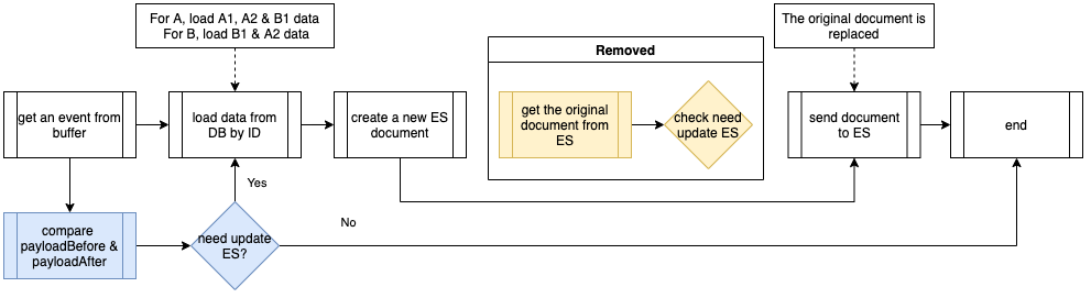
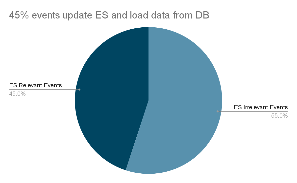
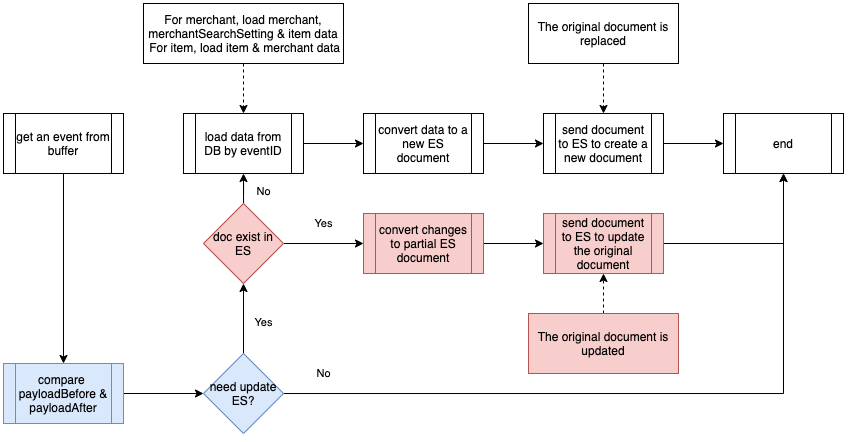
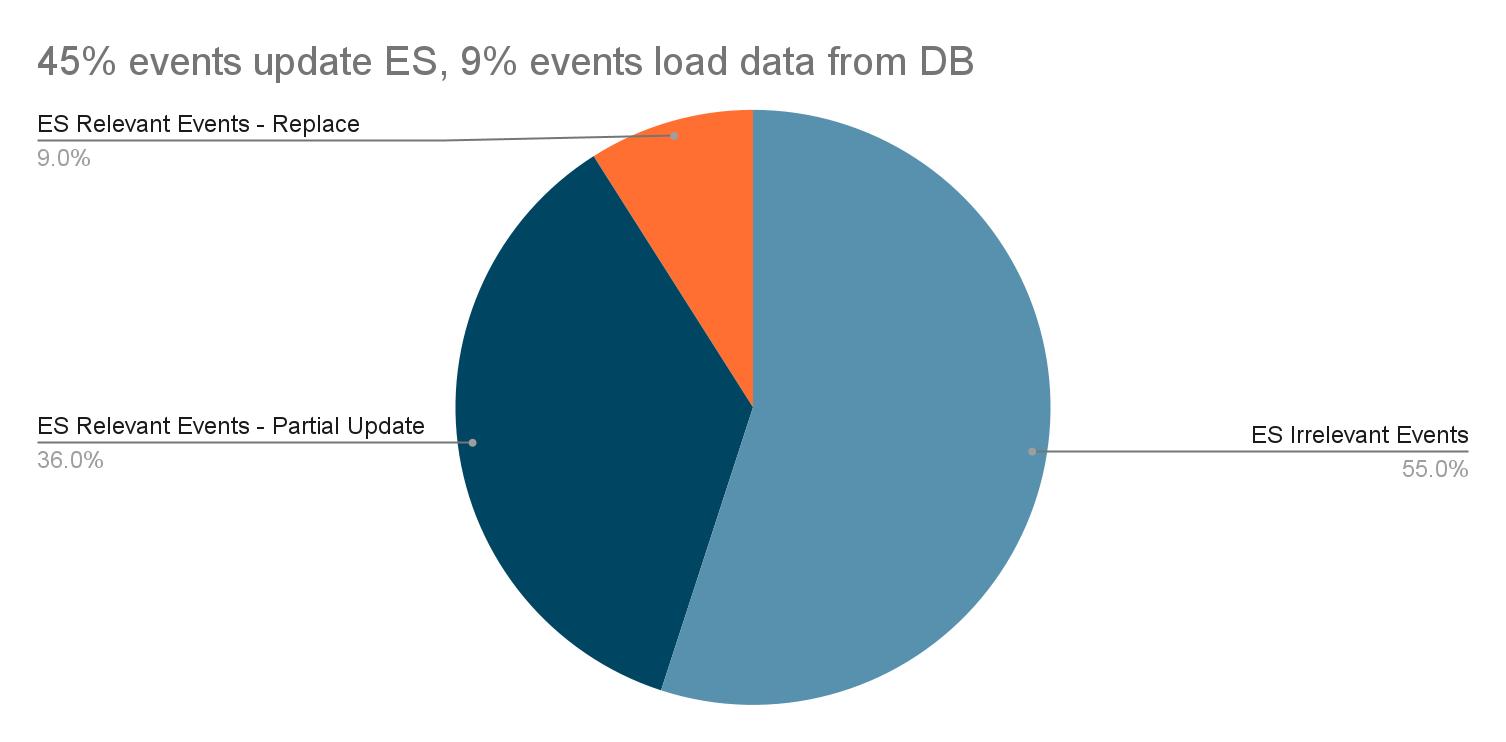
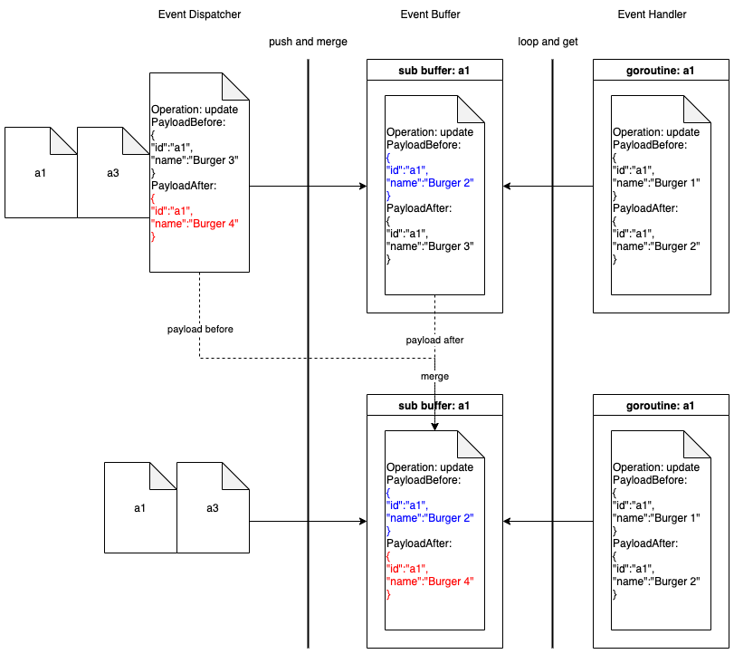
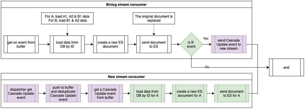
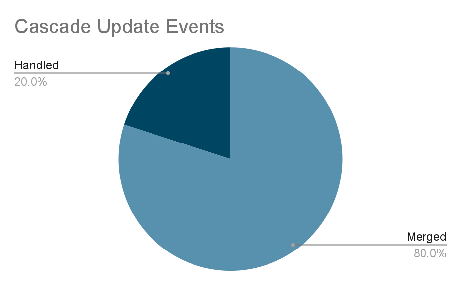
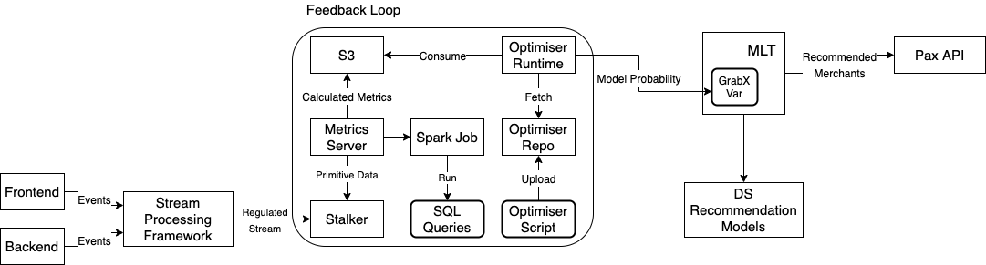

 .
.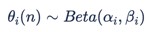 .
.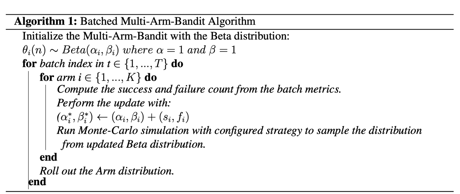
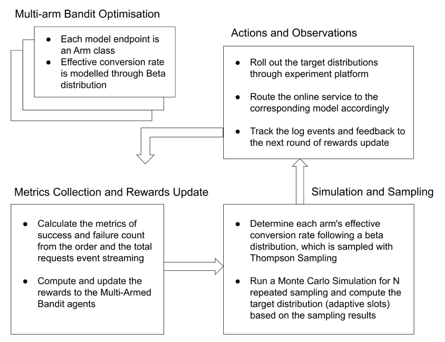
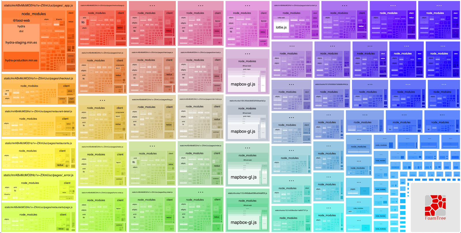
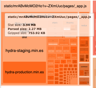

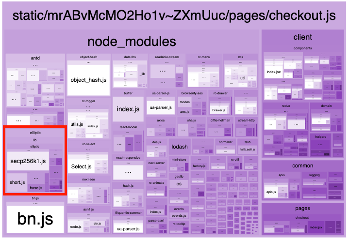


