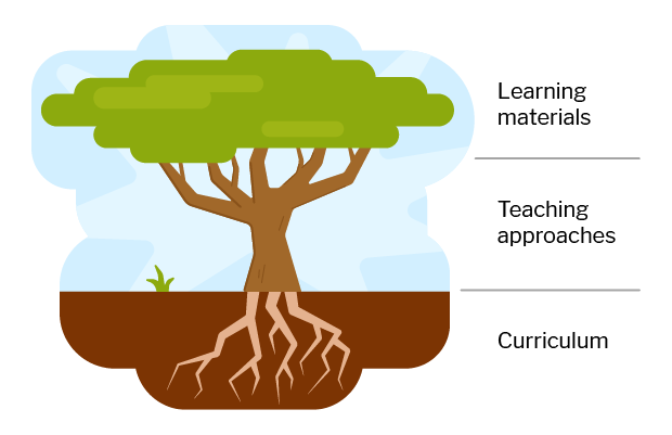
TOFU for Raspberry Pi Compute Module 4

Post Syndicated from Ashley Whittaker original https://www.raspberrypi.org/blog/tofu-for-raspberry-pi-compute-module-4/

In the latest issue of Custom PC magazine, Gareth Halfacree reviews Oratek’s TOFU, a carrier printed circuit board for Raspberry Pi Compute Module 4.

The launch of the Raspberry Pi Compute Module 4 family (reviewed in Issue 209) last year sparked an entirely unsurprising explosion of interest in designing carrier boards. This was aided in no small part by the Raspberry Pi Foundation’s decision to release its own in-house carrier board design under a permissive licence from which others could springboard with their own creations.

TOFU for Compute Module 4
Smartly designed with some clever features, the Tofu is a great carrier for a Raspberry Pi CM4 or compatible boards

Oratek doesn’t hide its inspiration. ‘Inspired by the official CM4IO board,’ chief executive Aurélien Essig openly admits, ‘it is intended for industrial applications. With user-friendly additions, it may also be used by enthusiasts looking for a compact yet complete solution to interface the many inputs and outputs of the single-board computer.’

The board is undeniably compact, although it bulks out when paired with the optional 3D-printed Switchblade Enclosure designed by Studio Raphaël Lutz. The reason for the name is that there are hinged lids on the top and bottom, which swing out for easy access, locking into place with small magnets when closed.

An optional adaptor converts the M.2 B-Key slot into an M-Key for NVMe storage

At least, that’s the theory. In practice, the magnets are a little weak; there’s also no way to fasten the lid shut beyond overtightening the screw in the corner. Otherwise, it’s a well-designed enclosure with top and bottom ventilation. Sadly, that’s not enough to prevent a Compute Module 4 from hitting its thermal throttle point under sustained heavy load, so you’ll need to budget for a third-party heatsink or fan accessory.

The Tofu board itself is well thought out, and finished in an attractive black. Two high-density connectors accept a Raspberry Pi Compute Module 4 board – or one of the increasing number of pin-compatible alternatives on the market, although you’ll need to provide your own mounting bolts.

TOFU for Compute Module 4 case
The 3D-printed case comes in an attractive ‘galaxy’ finish, but it isn’t cheap

The 90 x 90mm board then breaks out as many features of the computer-on-module as possible. The right side houses a Gigabit Ethernet port with Power-over-Ethernet (PoE) support if you add a Raspberry Pi PoE HAT or PoE+ HAT, two USB 2 Type-A ports, along with barrel-jack and 3.5mm terminal-block power inputs. These accept any input from 7.5V to 28V, which is brought out to an internal header for accessories that need more power than is available on the 40-pin general-purpose input/output (GPIO) port.

Meanwhile, the bottom has 22-pin connectors for Camera Serial Interface (CSI) and Display Serial Interface (DSI) peripherals, a full-sized HDMI port and an additional USB 2 port. These ports aren’t available outside the Switchblade Case by default, although a quick snap of the already-measured capped-off holes fixes that.

TOFU for Compute Module 4 case
Both the top and bottom rotate out of the way for easy access to the hardware inside

The left side includes a micro-SD slot for Compute Module 4 variants without on-board eMMC storage, plus a micro-SIM slot – hinting at another feature that becomes visible once the board is flipped. There’s also a USB Type-C port, which can be used for programming or as an On-The-Go (OTG) port. Oddly, there’s no cut-out at all for this in the Switchblade Case; if you want one, you’ll need to take a drill and file to it.

Turning over the board reveals the micro-SIM slot’s purpose. The Compute Module 4’s PCI-E lane is brought out to an M.2 B-Key slot, providing a connection for additional hardware including 3G/4G modems. For storage, you can use an optional adaptor board to convert it to M-Key for Non-Volatile Memory Express (NVMe) devices, with a spacer fitted for 2230, 2242, 2260, or 2280 form factor drives.

TOFU for Compute Module 4 ports
The Tofu has plenty of ports, but no USB 3

That’s not as flexible as it sounds, unfortunately. The spacer is soldered in place and needs to be chosen at the time of ordering. If you want to switch to a different-sized drive, you’ll need another adaptor.

There’s one other design point that makes the Tofu stand out: the inclusion of a user-replaceable fuse, a Littelfuse Nano 2 3.5A unit that was originally designed for automotive projects. 

While it’s primarily there for protection, it also enables you to cut off the on-board power supply when the board is driven through PoE. With the fuse in place, there’s clearly audible coil whine, which can be silenced by carefully popping the fuse out of its holder. Just remember to put it back in if you stop using PoE.

The biggest problem is price. At 99 CHF (around £78 ex VAT) you’ll be into triple figures by the time you’ve picked up a suitable power supply and Compute Module 4 board. The M.2 M-Key adaptor adds a further 19 CHF (around £15 ex VAT), and the Switchblade Case is another 35 CHF (around £28 ex VAT). If you have access to a 3D printer, you can opt to print the latter yourself, but you’ll still pay 8 CHF (around £6 ex VAT) for access to the files.

The Tofu is available to order now from oratek.com. Compatible Raspberry Pi Compute Module 4 boards can be found at the usual stockists.

Custom PC issue 217 out NOW!

You can read more features like this one in Custom PC issue 217, available directly from Raspberry Pi Press — we deliver worldwide.

custom pc front cover

And if you’d like a handy digital version of the magazine, you can also download issue 217 for free in PDF format.

The post TOFU for Raspberry Pi Compute Module 4 appeared first on Raspberry Pi.

Easily manage your data lake at scale using AWS Lake Formation Tag-based access control

Post Syndicated from Nivas Shankar original https://aws.amazon.com/blogs/big-data/easily-manage-your-data-lake-at-scale-using-tag-based-access-control-in-aws-lake-formation/

Thousands of customers are building petabyte-scale data lakes on AWS. Many of these customers use AWS Lake Formation to easily build and share their data lakes across the organization. As the number of tables and users increase, data stewards and administrators are looking for ways to manage permissions on data lakes easily at scale. Customers are struggling with “role explosion” and need to manage hundreds or even thousands of user permissions to control data access. For example, for an account with 1,000 resources and 100 principals, the data steward would have to create and manage up to 100,000 policy statements. Furthermore, as new principals and resources get added or deleted, these policies have to be updated to keep the permissions current.

Lake Formation Tag-based access control solves this problem by allowing data stewards to create LF-tags (based on their data classification and ontology) that can then be attached to resources. You can create policies on a smaller number of logical tags instead of specifying policies on named resources. LF-tags enable you to categorize and explore data based on taxonomies, which reduces policy complexity and scales permissions management. You can create and manage policies with tens of logical tags instead of the thousands of resources. LF-tags access control decouples policy creation from resource creation, which helps data stewards manage permissions on a large number of databases, tables, and columns by removing the need to update policies every time a new resource is added to the data lake. Finally, LF-tags access allows you to create policies even before the resources come into existence. All you have to do is tag the resource with the right LF-tags to ensure it is managed by existing policies.

This post focuses on managing permissions on data lakes at scale using LF-tags in Lake Formation. When it comes to managing data lake catalog tables from AWS Glue and administering permission to Lake Formation, data stewards within the producing accounts have functional ownership based on the functions they support, and can grant access to various consumers, external organizations, and accounts. You can now define LF-tags; associate at the database, table, or column level; and then share controlled access across analytic, machine learning (ML), and extract, transform, and load (ETL) services for consumption. LF-tags ensures that governance can be scaled easily by replacing the policy definitions of thousands of resources with a small number of logical tags.

LF-tags access has three main components:

  • Tag ontology and classification – Data stewards can define a LF-tag ontology based on data classification and grant access based on LF-tags to AWS Identity and Access Management (IAM) principals and SAML principals or groups
  • Tagging resources – Data engineers can easily create, automate, implement, and track all LF-tags and permissions against AWS Glue catalogs through the Lake Formation API
  • Policy evaluation – Lake Formation evaluates the effective permissions based on LF-tags at query time and allows access to data through consuming services such as Amazon Athena, Amazon Redshift Spectrum, Amazon SageMaker Data Wrangler, and Amazon EMR Studio, based on the effective permissions granted across multiple accounts or organization-level data shares

Solution overview

The following diagram illustrates the architecture of the solution described in this post.

In this post, we demonstrate how you can set up a Lake Formation table and create Lake Formation tag-based policies using a single account with multiple databases. We walk you through the following high-level steps:

  1. The data steward defines the tag ontology with two LF-tags: Confidential and Sensitive. Data with “Confidential = True” has tighter access controls. Data with “Sensitive = True” requires specific analysis from the analyst.
  2. The data steward assigns different permission levels to the data engineer to build tables with different LF-tags.
  3. The data engineer builds two databases: tag_database and col_tag_database. All tables in tag_database are configured with “Confidential = True”. All tables in the col_tag_database are configured with “Confidential = False”. Some columns of the table in col_tag_database are tagged with “Sensitive = True” for specific analysis needs.
  4. The data engineer grants read permission to the analyst for tables with specific expression condition “Confidential = True” and  “Confidential = FalseSensitive = True”.
  5. With this configuration, the data analyst can focus on performing analysis with the right data.

Provision your resources

This post includes an AWS CloudFormation template for a quick setup. You can review and customize it to suit your needs. The template creates three different personas to perform this exercise and copies the nyc-taxi-data dataset to your local Amazon Simple Storage Service (Amazon S3) bucket.

To create these resources, complete the following steps:

  1. Sign in to the AWS CloudFormation console in the us-east-1 Region.
  2. Choose Launch Stack:
  3. Choose Next.
  4. In the User Configuration section, enter password for three personas: DataStewardUserPassword, DataEngineerUserPassword and DataAnalystUserPassword.
  5. Review the details on the final page and select I acknowledge that AWS CloudFormation might create IAM resources.
  6. Choose Create.

The stack takes up to 5 minutes and creates all the required resources, including:

  • An S3 bucket
  • The appropriate Lake Formation settings
  • The appropriate Amazon Elastic Compute Cloud (Amazon EC2) resources
  • Three user personas with user ID credentials:
    • Data steward (administrator) – The lf-data-steward user has the following access:
      • Read access to all resources in the Data Catalog
      • Can create LF-tags and associate to the data engineer role for grantable permission to other principals
    • Data engineer – The lf-data-engineer user has the following access:
      • Full read, write, and update access to all resources in the Data Catalog
      • Data location permissions in the data lake
      • Can associate LF-tags and associate to the Data Catalog
      • Can attach LF-tags to resources, which provides access to principals based on any policies created by data stewards
    • Data analyst – The lf-data-analyst user has the following access:
      • Fine-grained access to resources shared by Lake Formation Tag-based access policies

Register your data location and create an LF-tag ontology

We perform this first step as the data steward user (lf-data-steward) to verify the data in Amazon S3 and the Data Catalog in Lake Formation.

  1. Sign in to the Lake Formation console as lf-data-steward with the password used while deploying the CloudFormation stack.
  2. In the navigation pane, under Permissions¸ choose Administrative roles and tasks.
  3. For IAM users and roles, choose the user lf-data-steward.
  4. Choose Save to add lf-data-steward as a Lake Formation admin.

    Next, we will update the Data catalog settings to use Lake Formation permission to control catalog resources instead of IAM based access control.
  5. In the navigation pane, under Data catalog¸ choose Settings.
  6. Uncheck Use only IAM access control for new databases.
  7. Uncheck Use only IAM access control for new tables in new databases.
  8. Click Save.

    Next, we need to register the data location for the data lake.
  9. In the navigation pane, under Register and ingest, choose Data lake locations.
  10. For Amazon S3 path, enter s3://lf-tagbased-demo-<<Account-ID>>.
  11. For IAM role¸ leave it as the default value AWSServiceRoleForLakeFormationDataAccess.
  12. Choose Register location.
    Next, we create the ontology by defining a LF-tag.
  13. Under Permissions in the navigation pane, under Administrative roles, choose LF-Tags.
  14. Choose Add LF-tags.
  15. For Key, enter Confidential.
  16. For Values, add True and False.
  17. Choose Add LF-tag.
  18. Repeat the steps to create the LF-tag Sensitive with the value True.
    You have created all the necessary LF-tags for this exercise.Next, we give specific IAM principals the ability to attach newly created LF-tags to resources.
  19. Under Permissions in the navigation pane, under Administrative roles, choose LF-tag permissions.
  20. Choose Grant.
  21. Select IAM users and roles.
  22. For IAM users and roles, search for and choose the lf-data-engineer role.
  23. In the LF-tag permission scope section, add the key Confidential with values True and False, and the key Sensitive with value True.
  24. Under Permissions¸ select Describe and Associate for LF-tag permissions and Grantable permissions.
  25. Choose Grant.

    Next, we grant permissions to lf-data-engineer to create databases in our catalog and on the underlying S3 bucket created by AWS CloudFormation.
  26. Under Permissions in the navigation pane, choose Administrative roles.
  27. In the Database creators section, choose Grant.
  28. For IAM users and roles, choose the lf-data-engineer role.
  29. For Catalog permissions, select Create database.
  30. Choose Grant.

    Next, we grant permissions on the S3 bucket (s3://lf-tagbased-demo-<<Account-ID>>) to the lf-data-engineer user.
  31. In the navigation pane, choose Data locations.
  32. Choose Grant.
  33. Select My account.
  34. For IAM users and roles, choose the lf-data-engineer role.
  35. For Storage locations, enter the S3 bucket created by the CloudFormation template (s3://lf-tagbased-demo-<<Account-ID>>).
  36. Choose Grant.
    Next, we grant lf-data-engineer grantable permissions on resources associated with the LF-tag expression Confidential=True.
  37. In the navigation pane, choose Data permissions.
  38. Choose Grant.
  39. Select IAM users and roles.
  40. Choose the role lf-data-engineer.
  41. In the LF-tag or catalog resources section, Select Resources matched by LF-Tags.
  42. Choose Add LF-Tag.
  43. Add the key Confidential with the values True.
  44. In the Database permissions section, select Describe for Database permissions and Grantable permissions.
  45. In the Table and column permissions section, select Describe, Select, and Alter for both Table permissions and Grantable permissions.
  46. Choose Grant.
    Next, we grant lf-data-engineer grantable permissions on resources associated with the LF-tag expression Confidential=False.
  47. In the navigation pane, choose Data permissions.
  48. Choose Grant.
  49. Select IAM users and roles.
  50. Choose the role lf-data-engineer.
  51. Select Resources matched by LF-tags.
  52. Choose Add LF-tag.
  53. Add the key Confidential with the values False.
  54. In the Database permissions section, select Describe for Database permissions and Grantable permissions.
  55. In the Table and column permissions section, do not select anything.
  56. Choose Grant.
    Next, we grant lf-data-engineer grantable permissions on resources associated with the LF-tag expression Confidential=False and Sensitive=True.
  57. In the navigation pane, choose Data permissions.
  58. Choose Grant.
  59. Select IAM users and roles.
  60. Choose the role lf-data-engineer.
  61. Select Resources matched by LF-tags.
  62. Choose Add LF-tag.
  63. Add the key Confidential with the values False.
  64. Choose Add LF-tag.
  65. Add the key Sensitive with the values True.
  66. In the Database permissions section, select Describe for Database permissions and Grantable permissions.
  67. In the Table and column permissions section, select Describe, Select, and Alter for both Table permissions and Grantable permissions.
  68. Choose Grant.

Create the Lake Formation databases

Now, sign in as lf-data-engineer with the password used while deploying the CloudFormation stack. We create two databases and attach LF-tags to the databases and specific columns for testing purposes.

Create your database and table for database-level access

We first create the database tag_database, the table source_data, and attach appropriate LF-tags.

  1. On the Lake Formation console, choose Databases.
  2. Choose Create database.
  3. For Name, enter tag_database.
  4. For Location, enter the S3 location created by the CloudFormation template (s3://lf-tagbased-demo-<<Account-ID>>/tag_database/).
  5. Deselect Use only IAM access control for new tables in this database.
  6. Choose Create database.

Next, we create a new table within tag_database.

  1. On the Databases page, select the database tag_database.
  2. Choose View Tables and click Create table.
  3. For Name, enter source_data.
  4. For Database, choose the database tag_database.
  5. For Data is located in, select Specified path in my account.
  6. For Include path, enter the path to tag_database created by the CloudFormation template (s3://lf-tagbased-demo-<<Account-ID>>/tag_database/).
  7. For Data format, select CSV.
  8. Under Upload schema, enter the following schema JSON:
    [
                   {
                        "Name": "vendorid",
                        "Type": "string"
                        
                        
                   },
                   {
                        "Name": "lpep_pickup_datetime",
                        "Type": "string"
                        
                        
                   },
                   {
                        "Name": "lpep_dropoff_datetime",
                        "Type": "string"
                        
                        
                   },
                      {
                        "Name": "store_and_fwd_flag",
                        "Type": "string"
                        
                        
                   },
                      {
                        "Name": "ratecodeid",
                        "Type": "string"
                        
                        
                   },
                      {
                        "Name": "pulocationid",
                        "Type": "string"
                        
                        
                   },
                   {
                        "Name": "dolocationid",
                        "Type": "string"
                        
                        
                   },
                      {
                        "Name": "passenger_count",
                        "Type": "string"
                        
                        
                   },
                   {
                        "Name": "trip_distance",
                        "Type": "string"
                        
                        
                   }, 
                      {
                        "Name": "fare_amount",
                        "Type": "string"
                        
                        
                   },
                   {
                        "Name": "extra",
                        "Type": "string"
                        
                        
                   },
                      {
                        "Name": "mta_tax",
                        "Type": "string"
                        
                        
                   },
                   {
                        "Name": "tip_amount",
                        "Type": "string"
                        
                        
                   },
                      {
                        "Name": "tolls_amount",
                        "Type": "string"
                        
                        
                   },
                   {
                        "Name": "ehail_fee",
                        "Type": "string"
                        
                        
                   }, 
                   {
                        "Name": "improvement_surcharge",
                        "Type": "string"
                        
                        
                   },
                   {
                        "Name": "total_amount",
                        "Type": "string"
                        
                        
                   },
                   {
                        "Name": "payment_type",
                        "Type": "string"
                        
                        
                   }
     
    ]
    

  9. Choose Upload.

After uploading the schema, the table schema should look like the following screenshot.

  1. Choose Submit.

Now we’re ready to attach LF-tags at the database level.

  1. On the Databases page, find and select tag_database.
  2. On the Actions menu, choose Edit LF-tags.
  3. Choose Assign new LF-tag.
  4. For Assigned keys¸ choose the Confidential LF-tag you created earlier.
  5. For Values, choose True.
  6. Choose Save.

This completes the LF-tag assignment to the tag_database database.

Create your database and table for column-level access

Now we repeat these steps to create the database col_tag_database and table source_data_col_lvl, and attach LF-tags at the column level.

  1. On the Databases page, choose Create database.
  2. For Name, enter col_tag_database.
  3. For Location, enter the S3 location created by the CloudFormation template (s3://lf-tagbased-demo-<<Account-ID>>/col_tag_database/).
  4. Deselect Use only IAM access control for new tables in this database.
  5. Choose Create database.
  6. On the Databases page, select your new database (col_tag_database).
  7. Choose View tables and Click Create table.
  8. For Name, enter source_data_col_lvl.
  9. For Database, choose your new database (col_tag_database).
  10. For Data is located in, select Specified path in my account.
  11. Enter the S3 path for col_tag_database (s3://lf-tagbased-demo-<<Account-ID>>/col_tag_database/).
  12. For Data format, select CSV.
  13. Under Upload schema, enter the following schema JSON:
    [
                   {
                        "Name": "vendorid",
                        "Type": "string"
                        
                        
                   },
                   {
                        "Name": "lpep_pickup_datetime",
                        "Type": "string"
                        
                        
                   },
                   {
                        "Name": "lpep_dropoff_datetime",
                        "Type": "string"
                        
                        
                   },
                      {
                        "Name": "store_and_fwd_flag",
                        "Type": "string"
                        
                        
                   },
                      {
                        "Name": "ratecodeid",
                        "Type": "string"
                        
                        
                   },
                      {
                        "Name": "pulocationid",
                        "Type": "string"
                        
                        
                   },
                   {
                        "Name": "dolocationid",
                        "Type": "string"
                        
                        
                   },
                      {
                        "Name": "passenger_count",
                        "Type": "string"
                        
                        
                   },
                   {
                        "Name": "trip_distance",
                        "Type": "string"
                        
                        
                   }, 
                      {
                        "Name": "fare_amount",
                        "Type": "string"
                        
                        
                   },
                   {
                        "Name": "extra",
                        "Type": "string"
                        
                        
                   },
                      {
                        "Name": "mta_tax",
                        "Type": "string"
                        
                        
                   },
                   {
                        "Name": "tip_amount",
                        "Type": "string"
                        
                        
                   },
                      {
                        "Name": "tolls_amount",
                        "Type": "string"
                        
                        
                   },
                   {
                        "Name": "ehail_fee",
                        "Type": "string"
                        
                        
                   }, 
                   {
                        "Name": "improvement_surcharge",
                        "Type": "string"
                        
                        
                   },
                   {
                        "Name": "total_amount",
                        "Type": "string"
                        
                        
                   },
                   {
                        "Name": "payment_type",
                        "Type": "string"
                        
                        
                   }
     
    ]
    

  14. Choose Upload.

After uploading the schema, the table schema should look like the following screenshot.

  1. Choose Submit to complete the creation of the table

Now you associate the  Sensitive=True LF-tag to the columns vendorid and fare_amount.

  1. On the Tables page, select the table you created (source_data_col_lvl).
  2. On the Actions menu, choose Edit Schema.
  3. Select the column vendorid and choose Edit LF-tags.
  4. For Assigned keys, choose Sensitive.
  5. For Values, choose True.
  6. Choose Save.

Repeat the steps for the Sensitive LF-tag update for fare_amount column.

  1. Select the column fare_amount and choose Edit LF-tags.
  2. Add the Sensitive key with value True.
  3. Choose Save.
  4. Choose Save as new version to save the new schema version with tagged columns.The following screenshot shows column properties with the LF-tags updated.
    Next we associate the Confidential=False LF-tag to col_tag_database. This is required for lf-data-analyst to be able to describe the database col_tag_database when logged in from Athena.
  5. On the Databases page, find and select col_tag_database.
  6. On the Actions menu, choose Edit LF-tags.
  7. Choose Assign new LF-tag.
  8. For Assigned keys¸ choose the Confidential LF-tag you created earlier.
  9. For Values, choose False.
  10. Choose Save.

Grant table permissions

Now we grant permissions to data analysts for consumption of the database tag_database and the table col_tag_database.

  1. Sign in to the Lake Formation console as lf-data-engineer.
  2. On the Permissions page, select Data Permissions
  3. Choose Grant.
  4. Under Principals, select IAM users and roles.
  5. For IAM users and roles, choose lf-data-analyst.
  6. Select Resources matched by LF-tags.
  7. Choose Add LF-tag.
  8. For Key, choose Confidential.
  9. For Values¸ choose True.
  10. For Database permissions, select Describe
  11. For Table permissions, choose Select and Describe.
  12. Choose Grant.

    This grants permissions to the lf-data-analyst user on the objects associated with the LF-tag Confidential=True (Database : tag_database)  to describe the database and the select permission on tables.Next, we repeat the steps to grant permissions to data analysts for LF-tag expression for Confidential=False . This LF-tag is used for describing the col_tag_database and the table source_data_col_lvl when logged in as lf-data-analyst from Athena. And so, we only grant describe access to the resources through this LF-tag expression.
  13. Sign in to the Lake Formation console as lf-data-engineer.
  14. On the Databases page, select the database col_tag_database.
  15. Choose Action and Grant.
  16. Under Principals, select IAM users and roles.
  17. For IAM users and roles, choose lf-data-analyst.
  18. Select Resources matched by LF-tags.
  19. Choose Add LF-tag.
  20. For Key, choose Confidential.
  21. For Values¸ choose False.
  22. For Database permissions, select Describe.
  23. For Table permissions, do not select anything.
  24. Choose Grant.

    Next, we repeat the steps to grant permissions to data analysts for LF-tag expression for Confidential=False and Sensitive=True. This LF-tag is used for describing the col_tag_database and the table source_data_col_lvl (Column level) when logged in as lf-data-analyst from Athena.
  25. Sign in to the Lake Formation console as lf-data-engineer.
  26. On the Databases page, select the database col_tag_database.
  27. Choose Action and Grant.
  28. Under Principals, select IAM users and roles.
  29. For IAM users and roles, choose lf-data-analyst.
  30. Select Resources matched by LF-tags.
  31. Choose Add LF-tag.
  32. For Key, choose Confidential.
  33. For Values¸ choose False.
  34. Choose Add LF-tag.
  35. For Key, choose Sensitive.
  36. For Values¸ choose True.
  37. For Database permissions, select Describe.
  38. For Database permissions, select Describe.
  39. For Table permissions, select Select and Describe.
  40. Choose Grant.

Run a query in Athena to verify the permissions

For this step, we sign in to the Athena console as lf-data-analyst and run SELECT queries against the two tables (source_data and source_data_col_lvl). We use our S3 path as the query result location (s3://lf-tagbased-demo-<<Account-ID>>/athena-results/).

  1. In the Athena query editor, choose tag_database in the left panel.
  2. Choose the additional menu options icon (three vertical dots) next to source_data and choose Preview table.
  3. Choose Run query.

The query should take a few minutes to run. The following screenshot shows our query results.

The first query displays all the columns in the output because the LF-tag is associated at the database level and the source_data table automatically inherited the LF-tag from the database tag_database.

  1. Run another query using col_tag_database and source_data_col_lvl.

The second query returns just the two columns that were tagged (Non-Confidential and Sensitive).

As a thought experiment, you can also check to see the Lake Formation Tag-based access policy behavior on columns to which the user doesn’t have policy grants.

When an untagged column is selected from the table source_data_col_lvl, Athena returns an error. For example, you can run the following query to choose untagged columns geolocationid:

SELECT geolocationid FROM "col_tag_database"."source_data_col_lvl" limit 10;

Extend the solution to cross-account scenarios

You can extend this solution to share catalog resources across accounts. The following diagram illustrates a cross-account architecture.

We describe this in more detail in a subsequent post.

Clean up

To help prevent unwanted charges to your AWS account, you can delete the AWS resources that you used for this walkthrough.

  1. Sign in as lf-data-engineer Delete the databases tag_database and col_tag_database
  2. Now, Sign in as lf-data-steward and clean up all the LF-tag Permissions, Data Permissions and Data Location Permissions that were granted above that were granted lf-data-engineer and lf-data-analyst.
  3. Sign in to the Amazon S3 console as the account owner (the IAM credentials you used to deploy the CloudFormation stack).
  4. Delete the following buckets:
    1. lf-tagbased-demo-accesslogs-<acct-id>
    2. lf-tagbased-demo-<acct-id>
  5. On the AWS CloudFormation console, delete the stack you created.
  6. Wait for the stack status to change to DELETE_COMPLETE.

Conclusion

In this post, we explained how to create a LakeFormation Tag-based access control policy in Lake Formation using an AWS public dataset. In addition, we explained how to query tables, databases, and columns that have LakeFormation Tag-based access policies associated with them.

You can generalize these steps to share resources across accounts. You can also use these steps to grant permissions to SAML identities. In subsequent posts, we highlight these use cases in more detail.


About the Authors

Sanjay Srivastava is a principal product manager for AWS Lake Formation. He is passionate about building products, in particular products that help customers get more out of their data. During his spare time, he loves to spend time with his family and engage in outdoor activities including hiking, running, and gardening.


Nivas Shankar is a Principal Data Architect at Amazon Web Services. He helps and works closely with enterprise customers building data lakes and analytical applications on the AWS platform. He holds a master’s degree in physics and is highly passionate about theoretical physics concepts.


Pavan Emani is a Data Lake Architect at AWS, specialized in big data and analytics solutions. He helps customers modernize their data platforms on the cloud. Outside of work, he likes reading about space and watching sports.


Bolster security with role-based access control in Amazon MWAA

Post Syndicated from Virendhar Sivaraman original https://aws.amazon.com/blogs/big-data/bolster-security-with-role-based-access-control-in-amazon-mwaa/

Amazon Studios invests in content that drives global growth of Amazon Prime Video and IMDb TV. Amazon Studios has a number of internal-facing applications that aim to streamline end-to-end business processes and information workflows for the entire content creation lifecycle. The Amazon Studios Data Infrastructure (ASDI) is a centralized, curated, and secure data lake that stores data, both in its original form and processed for analysis and machine learning (ML). The centralized ASDI is essential to break down data silos and combine different types of analytics, thereby allowing Amazon Studios to gain valuable insights, guide better business decisions, and innovate using the latest ML concepts.

What are the primary goals for Amazon MWAA adoption?

Amazon Managed Workflows for Apache Airflow (MWAA) is a fully managed service that makes it easier to run open-source versions of Apache Airflow on AWS. Builders at Amazon.com are engineering Amazon MWAA Directed Acyclic Graphs (DAGs) with prerequisites for provisioning the least privilege access model to the underlying services and resources, and restricting the blast radius of a given task.

Apache Airflow connections provide mechanisms for securely accessing the resources during DAG execution and are intended for coarse-grained access. Incorporating fine-grained access requires different mechanisms for implementation and code review prior to deployment. The additional challenge of codifying the infrastructure and stitching multiple systems together can also inject redundant activities when implementing fine-grained access patterns in Airflow.

How did Amazon achieve this goal?

The objective to enforce security for DAGs at its lowest possible granularity is done at the DAG’s task level. The solution aligns with integration of Amazon MWAA task security with AWS Identity and Access Management (IAM) service and AWS Security Token Service (AWS STS). The engineers customized the existing Airflow PythonOperators to tightly couple task access requirements to separately deployed IAM roles. The customized Airflow operator takes advantage of AWS STS to assume the associated IAM role. The temporary session created from AWS STS is used within PythonOperator to access the underlying resources required to run the task.

In this post, we discuss how to strengthen security in Amazon MWAA with role-based access control.

Prerequisites

To implement this solution, complete the following prerequisites:

  1. Create an AWS account with admin access.
  2. Create an Amazon MWAA environment.
    1. Note down the execution role ARN associated with the Amazon MWAA environment. This is available in the Permissions section of the environment.

  1. Create two Amazon Simple Storage Service (Amazon S3) buckets:
    1. s3://<AWS_ACCOUNT_ID>-<AWS_REGION>-mwaa-processed/
    2. s3://<AWS_ACCOUNT_ID>-<AWS_REGION>-mwaa-published/
  2. Create two IAM roles; one for each of the buckets:
    1. write_access_processed_bucket with the following policy:
{
    "Version": "2012-10-17",
    "Statement": [
        {
            "Sid": "VisualEditor0",
            "Effect": "Allow",
            "Action": [
                "s3:PutObject",
                "s3:DeleteObject"
            ],
            "Resource": "arn:aws:s3:::<AWS_ACCOUNT_ID>-<AWS_REGION>-mwaa-processed/*"
        }
    ]
}
    1. write_access_published_bucket with the following policy:
{
    "Version": "2012-10-17",
    "Statement": [
        {
            "Sid": "VisualEditor0",
            "Effect": "Allow",
            "Action": [
                "s3:PutObject",
                "s3:DeleteObject"
            ],
            "Resource": "arn:aws:s3:::<AWS_ACCOUNT_ID>-<AWS_REGION>-mwaa-published/*"
        }
    ]
}
  1. Update the trust relationship for the preceding two roles with the Amazon MWAA execution role obtained from Amazon MWAA environment page:
{
  "Version": "2012-10-17",
  "Statement": [
    {
      "Effect": "Allow",
      "Principal": {
        "AWS": [
          "arn:aws:iam::<AWS_ACCOUNT_ID>:assumed-role/<MWAA-EXECUTION_ROLE>/AmazonMWAA-airflow"
        ],
        "Service": "s3.amazonaws.com"
      },
      "Action": "sts:AssumeRole"
    }
  ]
}

In the preceding policy, replace AWS_ACCOUNT_ID and MWAA-EXECUTION_ROLE with the respective account number, region and Amazon MWAA execution role.

Run the DAG

The proposed DAG has two tasks that access each of the preceding buckets created:

  • Process task – Performs a task in the processed S3 bucket, which mocks a transformation using the Python sleep() function. The last step in this task adds a control file with the current timestamp.
  • Publish task – Performs a similar transformation in the published S3 bucket, which again mocks a transformation using the Python sleep() function. The last step in this task adds a control file with the current timestamp.

The fine-grained access restriction is enforced by a custom implementation of a widely used Airflow operator: PythonOperator. The custom PythonOperator negotiates with AWS STS to trade a session using the IAM role. The session is exclusively used by the tasks’ callable to access the underlying AWS resources. The following diagram shows the sequence of events.

The source code for the preceding implementation is available in the mwaa-rbac-task GitHub repository.

The code base is set up in the following location in Amazon S3, as seen from the Amazon MWAA environment on the Amazon MWAA console.

Run the DAG and monitor its progress, as shown in the following screenshot.

After you run the DAG, the following files are created with timestamps updated:

  • s3://<AWS_ACCOUNT_ID>-<AWS_REGION>-mwaa-processed/control_file/processed.json 
    	{
    		"processed_dt": "03/05/2021 01:03:58"
    	}

  • s3://<AWS_ACCOUNT_ID>-<AWS_REGION>-mwaa-published/control_file/published.json
    	{
    		"published_dt": "03/05/2021 01:04:12"
    	}

The change in the preceding control files reflects that the tasks in the DAGs enforced the policies defined for these tasks.

Create custom Airflow Operators to support least privilege access

You can extend the demonstrated methodology for enabling fine-grained access using a customized PythonOperator to other Airflow operators and sensors as needed. For more information about how to customize operators, see Creating a custom Operator.

Conclusion

In this post, we presented a solution to bolster security in Amazon MWAA with role-based access controls. You can extend the concept to other Airflow operators in order enhance the workflow security at the task level. In addition, using the AWS Cloud Development Kit (AWS CDK) can make provisioning the Amazon MWAA environment and fine-grained IAM task roles seamless. We look forward to sharing more about fine-grained access patterns for Airflow tasks in a future post.


About the Author

Kishan Desai is a Data Engineer at Amazon Studios building a data platform to support the content creation process. He is passionate about building flexible and modular systems on AWS using serverless paradigms. Outside of work, Kishan enjoys learning new technologies, watching sports, experiencing SoCal’s great food, and spending quality time with friends and family.


Virendhar (Viru) Sivaraman is a strategic Big Data & Analytics Architect with Amazon Web Services. He is passionate about building scalable big data and analytics solutions in the cloud. Besides work, he enjoys spending time with family, hiking & mountain biking.

[$] Hardening virtio

Post Syndicated from original https://lwn.net/Articles/865216/rss

Traditionally, in virtualized environments, the host is trusted by its
guests, and must
protect itself from potentially malicious guests. With initiatives
like confidential computing, this rule is extended in the other direction: the
guest no longer trusts the host. This change of paradigm requires
adding boundary defenses in places where there have been none before.
Recently, Andi Kleen submitted a patch
set
attempting to add the needed protections in virtio. The discussion
that resulted from this patch set highlighted the need to secure
virtio for a wider range of use cases.

Classifying Millions of Amazon items with Machine Learning, Part I: Event Driven Architecture

Post Syndicated from Mahmoud Abid original https://aws.amazon.com/blogs/architecture/classifying-millions-of-amazon-items-with-machine-learning-part-i-event-driven-architecture/

As part of AWS Professional Services, we work with customers across different industries to understand their needs and supplement their teams with specialized skills and experience.

Some of our customers are internal teams from the Amazon retail organization who request our help with their initiatives. One of these teams, the Global Environmental Affairs team, identifies the number of electronic products sold. Then they classify these products according to local laws and accurately report this data to regulators. This process covers the products’ end-of-life costs and ensures a high quality of recycling.

These electronic products have classification codes that differ from country to country, and these codes change according to each country’s latest regulations. This poses a complex technical problem. How do we automate our compliance teams’ work to efficiently and accurately classify over three million product classifications every month, in more than 38 countries, while also complying with evolving classification regulations?

To solve this problem, we used Amazon Machine Learning (Amazon ML) capabilities to build a resilient architecture. It ingests and processes data, trains ML models, and predicts (also known as inference workflow) monthly sales data for all countries concurrently.

In this post, we outline how we used AWS Lambda, Amazon EventBridge, and AWS Step Functions to build a scalable and cost-effective solution. We’ll also show you how to keep the data secure while processing it in Amazon ML flows.

Solution overview

Our solution consists of three main parts, which are summarized here and detailed in the following sections:

  1. Training the ML models
  2. Evaluating their performance
  3. Using them to run an inference workflow (in other words, label) the sold items with the correct classification codes

Training the Amazon ML model

For training our Amazon ML model, we use the architecture in Figure 1. It starts with a periodic query against the Amazon.com data warehouse in Amazon Redshift.

Training workflow

Figure 1. Training workflow

  1. A labeled dataset containing pre-recorded classification codes is extracted from Amazon Redshift. This dataset is stored in an Amazon Simple Storage Service (Amazon S3) bucket and split up by country. The data is encrypted at rest with server-side encryption using an AWS Key Management Service (AWS KMS) key. This is also known as server-side encryption with AWS KMS (SSE-KMS). The extraction query uses the AWS KMS key to encrypt the data when storing it in the S3 bucket.
  2. Each time a country’s dataset is uploaded to the S3 bucket, a message is sent to an Amazon Simple Queue Service (Amazon SQS) queue. This prompts a Lambda function. We use Amazon SQS to ensure resiliency. If the Lambda function fails, the message will be tried again automatically. Overall, the message is either processed successfully, or ends up in a dead letter queue that we monitor (not displayed in Figure 1).
  3. If the message is processed successfully, the Lambda function generates necessary input parameters. Then it starts a Step Functions workflow execution for the training process.
  4. The training process involves orchestrating Amazon SageMaker Processing jobs to prepare the data. Once the data is prepared, a hyperparameter optimization job invokes multiple training jobs. These run in parallel with different values from a range of hyperparameters. The model that performs the best is chosen to move forward.
  5. After the model is trained successfully, an EventBridge event is prompted, which will be used to invoke the performance comparison process.

Comparing performance of Amazon ML models

Because Amazon ML models are automatically trained periodically, we want to assess their performance automatically too. Newly created models should perform better than their predecessors. To measure this, we use the flow in Figure 2.

Model performance comparison workflow

Figure 2. Model performance comparison workflow

  1. The flow is activated by the EventBridge event at the end of the training flow.
  2. A Lambda function gathers the necessary input parameters and uses them to start an inference workflow, implemented as a Step Function.
  3. The inference workflow use SageMaker Processing jobs to prepare a new test dataset. It performs predictions using SageMaker Batch Transform jobs with the new model. The test dataset is a labeled subset that was not used in model training. Its prediction gives an unbiased estimation of the model’s performance, proving that the model can generalize.
  4. After the inference workflow is completed and the results are stored on Amazon S3, an EventBridge event is performed, which prompts another Lambda function. This function runs the performance comparison Step Function.
  5. The performance comparison workflow uses a SageMaker Processing job to analyze the inference results and calculate its performance score based on ground truth. For each country, the job compares the performance of the new model with the performance of the last used model to determine which one was best, otherwise known as the “winner model.” The metadata of the winner model is saved in an Amazon DynamoDB table so it can be queried and used in the next production inference job.
  6. At the end of the performance comparison flow, an informational notification is sent to an Amazon Simple Notification Service (Amazon SNS) topic, which will be received by the MLOps team.

Running inference

The inference flow starts with a periodic query against the Amazon.com data warehouse in Amazon Redshift, as shown in Figure 3.

Inference workflow

Figure 3. Inference workflow

  1. As with training, the dataset is extracted from Amazon Redshift, split up by country, and stored in an S3 bucket and encrypted at rest using the AWS KMS key.
  2. Every country dataset upload prompts a message to an SQS queue, which invokes a Lambda function.
  3. The Lambda function gathers necessary input parameters and starts a workflow execution for the inference process. This is the same Step Function we used in the performance comparison. Now it runs against the real dataset instead of the test set.
  4. The inference Step Function orchestrates the data preparation and prediction using the winner model for each country, as stored in the model performance DynamoDB table. The predictions are uploaded back to the S3 bucket to be further consumed for reporting.
  5. Lastly, an Amazon SNS message is sent to signal completion of the inference flow, which will be received by different stakeholders.

Data encryption

One of the key requirements of this solution was to provide least privilege access to all data. To achieve this, we use AWS KMS to encrypt all data as follows:

Restriction of data decryption permissions

Figure 4. Restriction of data decryption permissions

Conclusion

In this post, we outline how we used a serverless architecture to handle the end-to-end flow of data extraction, processing, and storage. We also talk about how we use this data for model training and inference.

With this solution, our customer team onboarded 38 countries and brought 60 Amazon ML models to production to classify 3.3 million items on a monthly basis.

In the next post, we show you how we use AWS Developer Tools to build a comprehensive continuous integration/continuous delivery (CI/CD) pipeline that safeguards the code behind this solution.


Choosing between AWS services for streaming data workloads

Post Syndicated from James Beswick original https://aws.amazon.com/blogs/compute/choosing-between-aws-services-for-streaming-data-workloads/

Traditionally, streaming data can be complex to manage due to the large amounts of data arriving from many separate sources. Managing fluctuations in traffic and durably persisting messages as they arrive is a non-trivial task. Using a serverless approach, AWS provides a number of services that help manage large numbers of messages, alleviating much of the infrastructure burden.

In this blog post, I compare several AWS services and how to choose between these options in streaming data workloads.

Comparing Amazon Kinesis Data Streams with Amazon SQS queues

While you can use both services to decouple data producers and consumers, each is suited to different types of workload. Amazon SQS is primarily used as a message queue to store messages durably between distributed services. Amazon Kinesis is primarily intended to manage streaming big data.

Kinesis supports ordering of records and the ability for multiple consumers to read messages from the same stream concurrently. It also allows consumers to replay messages from up to 7 days previously. Scaling in Kinesis is based upon shards and you must reshard to scale a data stream up or down.

With SQS, consumers pull data from a queue and it’s hidden from other consumers until processed successfully (known as a visibility timeout). Once a message is processed, it’s deleted from the queue. A queue may have multiple consumers but they all receive separate batches of messages. Standard queues do not provide an ordering guarantee but scaling in SQS is automatic.

Amazon Kinesis Data Streams

Amazon SQS

Ordering guarantee Yes, by shard No for standard queues; FIFO queues support ordering by group ID.
Scaling Resharding required to provision throughput Automatic for standard queues; up to 30,000 message per second for FIFO queues (more details).
Exactly-once delivery No No for standard queues; Yes for FIFO queues.
Consumer model Multiple concurrent Single consumer
Configurable message delay No Up to 15 minutes
Ability to replay messages Yes No
Encryption Yes Yes
Payload maximum 1 MB per record 256 KB per message
Message retention period 24 hours (default) to 365 days (additional charges apply) 1 minute to 14 days. 4 days is the default
Pricing model Per shard hour plus PUT payload unit per million. Additional charges for some features No minimum; $0.24-$0.595 per million messages, depending on Region and queue type
AWS Free Tier included No Yes, 1 million messages per month – see details
Typical use cases

Real-time metrics/reporting

Real-time data analytics

Log and data feed processing

Stream processing

Application integration

Asynchronous processing

Batching messages/smoothing throughput

Integration with Kinesis Data Analytics Yes No
Integration with Kinesis Data Firehose Yes No

While some functionality of both services is similar, Kinesis is often a better fit for many streaming workloads. Kinesis has a broader range of options for ingesting large amounts of data, such as the Kinesis Producer Library and Kinesis Aggregation Library. You can also use the PutRecords API to send up to 500 records (up to a maximum 5 MiB) per request.

Additionally, it has powerful integrations not available to SQS. Amazon Kinesis Data Analytics allows you to transform and analyze streaming data with Apache Flink. You can also use streaming SQL to run windowed queries on live data in near-real time. You can also use Amazon Kinesis Data Firehose as a consumer for Amazon Kinesis Data Streams, which is also not available to SQS queues.

Choosing between Kinesis Data Streams and Kinesis Data Firehose

Both of these services are part of Kinesis but they have different capabilities and target use-cases. Kinesis Data Firehose is a fully managed service that can ingest gigabytes of data from a variety of producers. When Kinesis Data Streams is the source, it automatically scales up or down to match the volume of data. It can optionally process records as they arrive with AWS Lambda and deliver batches of records to services like Amazon S3 or Amazon Redshift. Here’s how the service compares with Kinesis Data Streams:

Kinesis Data Streams

Kinesis Data Firehose

Scaling Resharding required Automatic
Supports compression No Yes (GZIP, ZIP, and SNAPPY)
Latency ~200 ms per consumer (~70 ms if using enhanced fan-out) Seconds (depends on buffer size configuration); minimum buffer window is 60 seconds
Retention 1–365 days None
Message replay Yes No
Quotas See quotas See quotas
Ingestion capacity Determined by number of shards (1,000 records or 1 MB/s per shard) No limit if source is Kinesis Data Streams; otherwise see quota page
Producer types

AWS SDK or AWS CLI

Kinesis Producer Library

Kinesis Agent

Amazon CloudWatch

Amazon EventBridge

AWS IoT Core

AWS SDK or AWS CLI

Kinesis Producer Library

Kinesis Agent

Amazon CloudWatch

Amazon EventBridge

AWS IoT Core

Kinesis Data Streams

Number of consumers Multiple, sharing 2 MB per second per shard throughput One per delivery stream
Consumers

AWS Lambda

Kinesis Data Analytics

Kinesis Data Firehose

Kinesis Client Library

Amazon S3

Amazon Redshift

Amazon Elasticsearch Service

Third-party providers

HTTP endpoints

Pricing Hourly charge plus data volume. Some features have additional charges – see pricing Based on data volume, format conversion and VPC delivery – see pricing

The needs of your workload determine the choice between the two services. To prepare and load data into a data lake or data store, Kinesis Data Firehose is usually the better choice. If you need low latency delivery of records and the ability to replay data, choose Kinesis Data Streams.

Using Kinesis Data Firehose to prepare and load data

Kinesis Data Firehose buffers data based on two buffer hints. You can configure a time-based buffer from 1-15 minutes and a volume-based buffer from 1-128 MB. Whichever limit is reached first causes the service to flush the buffer. These are called hints because the service can adjust the settings if data delivery falls behind writing to the stream. The service raises the buffer settings dynamically to allow the service to catch up.

This is the flow of data in Kinesis Data Firehose from a data source through to a destination, including optional settings for a delivery stream:

Kinesis Dat Firehose flow

  1. The service continuously loads from the data source as it arrives.
  2. The data transformation Lambda function processes individual records and returns these to the service.
  3. Transformed records are delivered to the destination once the buffer size or buffer window is reached.
  4. Any records that could not be delivered to the destination are written to an intermediate S3 bucket.
  5. Any records that cannot be transformed by the Lambda function are written to an intermediate S3 bucket.
  6. Optionally, the original, untransformed records are written to an S3 bucket.

Data transformation using a Lambda function

The data transformation process enables you to modify the contents of individual records. Kinesis Data Firehose synchronously invokes the Lambda function with a batch of records. Your custom code modifies the records and then returns an array of transformed records.

Transformed records

The incoming payload provides the data attribute in base64 encoded format. Once the transformation is complete, the returned array must include the following attributes per record:

  • recordId: This must match the incoming recordId to enable the service to map the new data to the record.
  • result: “Ok”, “Dropped”, or “ProcessingFailed”. Dropped means that your logic has intentionally removed the record whereas ProcessingFailed indicates that an error has occurred.
  • data: The transformed data must be base64 encoded.

The returned array must be the same length as the incoming array. The Alleycat example application uses the following code in the data transformation function to add a calculated field to the record:

exports.handler = async (event) => {
    const output = event.records.map((record) => {
        
      // Extract JSON record from base64 data
      const buffer = Buffer.from(record.data, 'base64').toString()
      const jsonRecord = JSON.parse(buffer)

	// Add the calculated field
	jsonRecord.output = ((jsonRecord.cadence + 35) * (jsonRecord.resistance + 65)) / 100

	// Convert back to base64 + add a newline
	const dataBuffer = Buffer.from(JSON.stringify(jsonRecord) + '\n', 'utf8').toString('base64')

       return {
            recordId: record.recordId,
            result: 'Ok',
            data: dataBuffer
        }
    })
    
    console.log(`Output records: ${output.length}`)
    return { records: output }
}

Comparing scaling and throughput with Kinesis Data Streams and Kinesis Data Firehose

Kinesis Data Firehose manages scaling automatically. If the data source is a Kinesis Data Stream, there is no limit to the amount of data the service can ingest. If the data source is a direct put using the PutRecordBatch API, there are soft limits of up to 500,000 records per second, depending upon the Region. See the Kinesis Data Firehose quota page for more information.

Kinesis Data Firehose invokes a Lambda transformation function synchronously and scales up the function as the number of records in the stream grows. When the destination is S3, Amazon Redshift, or the Amazon Elasticsearch Service, Kinesis Data Firehose allows up to five outstanding Lambda invocations per shard. When the destination is Splunk, the quota is 10 outstanding Lambda invocations per shard.

With Kinesis Data Firehose, the buffer hints are the main controls for influencing the rate of data delivery. You can decide between more frequent delivery of small batches of message or less frequent delivery of larger batches. This can impact the PUT cost when using a destination like S3. However, this service is not intended to provide real-time data delivery due to the transformation and batching processes.

With Kinesis Data Streams, the number of shards in a stream determines the ingestion capacity. Each shard supports ingesting up to 1,000 messages or 1 MB per second of data. Unlike Kinesis Data Firehose, this service does not allow you to transform records before delivery to a consumer.

Data Streams has additional capabilities for increasing throughput and reducing the latency of data delivery. The service invokes Lambda consumers every second with a configurable batch size of messages. If the consumers are falling behind data production in the stream, you can increase the parallelization factor. By default, this is set to 1, meaning that each shard has a single instance of a Lambda function it invokes. You can increase this up to 10 so that multiple instances of the consumer function process additional batches of messages.

Increase the parallelization factor

Data Streams consumers use a pull model over HTTP to fetch batches of records, operating in serial. A stream with five standard consumers averages 200 ms of latency each, taking up to 1 second in total. You can improve the overall latency by using enhanced fan-out (EFO). EFO consumers use a push model over HTTP/2 and are independent of each other.

With EFO, all five consumers in the previous example receive batches of messages in parallel using dedicated throughput. The overall latency averages 70 ms and typically data delivery speed is improved by up to 65%. Note that there is an additional charge for this feature.

Kinesis Data Streams EFO consumers

Conclusion

This blog post compares different AWS services for handling streaming data. I compare the features of SQS and Kinesis Data Streams, showing how ordering, ingestion throughput, and multiple consumers often make Kinesis the better choice for streaming workloads.

I compare Data Streams and Kinesis Data Firehose and show how Kinesis Data Firehose is the better option for many data loading operations. I show how the data transformation process works and the overall workflow of a Kinesis Data Firehose stream. Finally, I compare the scaling and throughput options for these two services.

For more serverless learning resources, visit Serverless Land.

Security updates for Monday

Post Syndicated from original https://lwn.net/Articles/865680/rss

Security updates have been issued by Debian (ansible and bluez), Fedora (curl, kernel, mod_auth_openidc, rust-rav1e, and webkit2gtk3), Mageia (kernel and kernel-linus), openSUSE (php7 and python-reportlab), Oracle (ruby:2.7), Red Hat (microcode_ctl), SUSE (fastjar, kvm, mariadb, php7, php72, php74, and python-Pillow), and Ubuntu (docker.io).

Bring on the documentation

Post Syndicated from Alasdair Allan original https://www.raspberrypi.org/blog/bring-on-the-documentation/

I joined Raspberry Pi eighteen months ago and spent my first year here keeping secrets and writing about Raspberry Silicon, and the chip that would eventually be known as RP2040. This is all (largely) completed work: Raspberry Pi Pico made its way out into the world back in January, and our own Raspberry Silicon followed last month.

The question is then, what have I done for you lately?

The Documentation

Until today our documentation for the “big” boards — as opposed to Raspberry Pi Pico — lived in a Github repository and was written in Github-flavoured Markdown. From there our documentation site was built from the Markdown source, which was pulled periodically from the repository, run through a script written many years ago which turned it into HTML, and then deployed onto our website.

This all worked really rather well in the early days of Raspberry Pi.

The old-style documentation

The documentation repository itself has been left to grow organically. When I arrived here, it needed to be restructured, and a great deal of non-Raspberry Pi specific documentation needed to be removed, while other areas were underserved and needed to be expanded. The documentation was created when there was a lot less third-party content around to support the Raspberry Pi, so a fair bit of it really isn’t that relevant anymore, and is better dealt with elsewhere on the web. And the structure was a spider’s web that, in places, made very little sense.

Frankly, it was all in a bit of a mess.

Enter the same team of folks that built the excellent PDF-based documentation for Raspberry Pi Pico and RP2040. The PDF documentation was built off an Asciidoc-based toolchain, and we knew from the outset that we’d want to migrate the Markdown-based documentation to Asciidoc. It’d offer us more powerful tools going forwards, and a lot more flexibility.

After working through the backlog of community pull requests, we took a snapshot of the current Markdown-based repository and built out a toolchain. A lot of which we intended to, and did, throw away after converting the Markdown to Asciidoc as our “source of truth.” This didn’t happen without a bit of a wrench; nobody throws working code away lightly. But it did mean we’d reached the point of no return.

The next generation of documentation

The result of our new documentation project launches today.

The new-look documentation

The new documentation site is built and deployed directly from the documentation repository using Github Actions when someone pushes to the master branch. However we’ll mostly be working on the develop branch in the repository, which is the default branch you’ll now get when you take a fresh checkout, and also the branch you should target for your pull requests.

We’ve always taken pull requests against the Markdown-based source behind our documentation site. Over the years as the documentation set has grown there have been hundreds of community contributors, who have made over 1,200 individual pull requests, ranging from fixing small typos, to contributing whole new sections.

With the introduction of the new site, we’re going to continue to take pull requests against the new Asciidoc-based documentation. However, we’re going to be a bit more targeted around what we’ll to accept into the documentation, and will be looking to keep the repository focussed on Raspberry Pi-specific things, rather than having generic Linux tutorial content.

The documentation itself will remain under a Creative Commons Attribution-Sharealike (CC BY-SA 4.0) license.

Product Information Portal

Supporting our customers in the best way we can when they build products around Raspberry Pi computers is important to us. A big part of this is being able to get customers access to the right documents easily. So alongside the new-look documentation, we have revamped how our customers (that’s you) get access to the documents you need for commercial applications of Raspberry Pi.

The Product Information Portal, or PIP as we’ve come to refer to it here at Pi Towers, is where documents such as regulatory paperwork, product change notices, and white papers will be stored and accessed from now on.

The new Product Information Portal (PIP)

PIP has three tiers of document type: those which are publicly available; restricted documents that require a customer to sign up for a free account; and confidential documents which require a customer’s company to enter into a confidentiality agreement with Raspberry Pi.

PIP will also be a way for customers to get updates on products, allowing customers with a user account to subscribe to products, and receive email updates should there be a product change, regulatory update, or white paper release.

The portal can be found at pip.raspberrypi.org and will be constantly updated as new documents become available.

Where next?

I’m hoping that everyone that has contributed to the documentation over the years will see the new site as a big step towards making our documentation more accessible – and, as ever, we accept pull requests. However, if you’re already a contributor, the easiest thing to do is to take a fresh checkout of the repository, because things have changed a lot today.

Big changes to the look-and-feel of the documentation site

This isn’t the end. Instead, it’s the beginning of a journey to try and pull together our documentation into something that feels a bit more cohesive. While the documentation set now looks, and feels, a lot better and is (I think) a lot easier to navigate if you don’t know it well, there is still a lot of pruning and re-writing ahead of me. But we’ve reached the stage where I’m happy, and want to, work on that in public so the community can see how things are changing and can help out.

The post Bring on the documentation appeared first on Raspberry Pi.

Defeating Microsoft’s Trusted Platform Module

Post Syndicated from Bruce Schneier original https://www.schneier.com/blog/archives/2021/08/defeating-microsofts-trusted-platform-module.html

This is a really interesting story explaining how to defeat Microsoft’s TPM in 30 minutes — without having to solder anything to the motherboard.

Researchers at the security consultancy Dolos Group, hired to test the security of one client’s network, received a new Lenovo computer preconfigured to use the standard security stack for the organization. They received no test credentials, configuration details, or other information about the machine.

They were not only able to get into the BitLocker-encrypted computer, but then use the computer to get into the corporate network.

It’s the “evil maid attack.” It requires physical access to your computer, but you leave it in your hotel room all the time when you go out to dinner.

Original blog post.

The collective thoughts of the interwebz

By continuing to use the site, you agree to the use of cookies. more information

The cookie settings on this website are set to "allow cookies" to give you the best browsing experience possible. If you continue to use this website without changing your cookie settings or you click "Accept" below then you are consenting to this.

Close