Tag Archives: AWS Big Data

Implementing multi-tenant patterns in Amazon Redshift using data sharing

2021-02-12 Rajesh Francis

Post Syndicated from Rajesh Francis original https://aws.amazon.com/blogs/big-data/implementing-multi-tenant-patterns-in-amazon-redshift-using-data-sharing/

Software service providers offer subscription-based analytics capabilities in the cloud with Analytics as a Service (AaaS), and increasingly customers are turning to AaaS for business insights. A multi-tenant storage strategy allows the service providers to build a cost-effective architecture to meet increasing demand.

Multi-tenancy means a single instance of software and its supporting infrastructure is shared to serve multiple customers. For example, a software service provider could generate data that is housed in a single data warehouse cluster, but accessed securely by multiple customers. This storage strategy offers an opportunity to centralize management of data, simplify ETL processes, and optimize costs. However, service providers have to constantly balance between cost and providing a better user experience for their customers.

With the new data sharing feature, you can use Amazon Redshift to scale and meet both objectives of managing costs by simplifying storage and ETL pipelines while still providing consistent performance to customers. You can ingest data into a cluster designated as a producer cluster, and share this live data with one or more consumer clusters. Clusters accessing this shared data are isolated from each other, therefore performance of a producer cluster isn’t impacted by workloads on consumer clusters. This enables consuming clusters to get consistent performance based on individual compute capacity.

In this post, we focus on various AaaS patterns, and discuss how you can use data sharing in a multi-tenant architecture to scale for virtually unlimited users. We discuss detailed steps to use data sharing with different storage strategies.

Multi-tenant storage patterns

Multi-tenant storage patterns help simplify the architecture and long-term maintenance of the analytics platform. In a multi-tenant strategy, data is stored centrally in a single cluster for all tenants, enabling simplification of the ETL ingestion pipeline and data management. In the previously published whitepaper SaaS Storage Strategies, various models of storage and benefits are covered for a single cluster scenario.

The three strategies you can choose from are:

Pool model – Data is stored in a single database schema for all tenants, and a new column (tenant_id) is used to scope and control access to individual tenant data. Access to the multi-tenant data is controlled using views built on the tables.
Bridge model – Storage and access to data for each tenant is controlled at individual schema level in the same database.
Silo model – Storage and access control to data for each tenant is maintained in separate databases

The following diagram illustrates the architecture of these multi-tenant storage strategies.

In the following sections, we will discuss how these multi-tenant strategies can be implemented using Amazon Redshift data sharing feature with a multi-cluster architecture.

Scaling your multi-tenant architecture using data sharing

AaaS providers implementing multi-tenant architectures were previously limited to resources of a single cluster to meet the compute and concurrency requirements of users across all the tenants. As the number of tenants increased, you could either turn on concurrency scaling or create additional clusters. However, the addition of new clusters means additional ingestion pipelines and increased operational overhead.

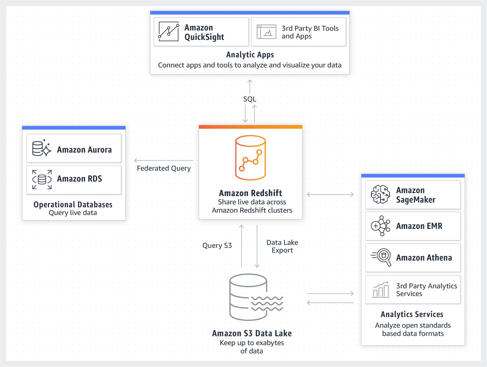
With data sharing in Amazon Redshift, you can easily and securely share data across clusters. Data ingested into the producer cluster is shared with one or more consumer clusters, which allows total separation of ETL and BI workloads. Several consumer clusters can read data from the managed storage of a producer cluster. This enables instant, granular, and high-performance access without data copies and movement. Workloads accessing shared data are isolated from each other and the producer. You can distribute workloads across multiple clusters while simplifying and consolidating the ETL ingestion pipeline into one main producer cluster, providing optimal price for performance.

Consumer clusters can in turn be producers for the data sets they own. Customers can optimize costs even further by collocating multiple tenants on the same consumer cluster. For instance, you can group low volume tier 3 tenants into a single consumer cluster to provider a lower cost offering, while high volume tier 1 tenants get their own isolated compute clusters. Consumer clusters can be created in the same account as producer or in a different AWS account. With this you can have separate billing for the consumer clusters, where you can chargeback to the business group that uses the consumer cluster or even allow your customers to use their own Redshift cluster in their account, so they pay for usage of the consumer cluster. The following diagram shows the difference in ETL and consumer access patterns in a multi-tenant architecture using data sharing versus a single cluster approach without data sharing.

Consumer clusters can in turn be producers for the data sets they own.

Multi-tenant architecture with data sharing compared to single cluster approach

Creating a multi-tenant architecture for an AaaS solution

For this post, we use a simple data model with a fact and a dimension table to demonstrate how to leverage data sharing to design a scalable multi-tenant AaaS solution. We cover detailed steps involved for each storage strategy using this data model. The tables are as follows:

Customer – dimension table containing customer details
Sales – fact table containing sales transactions

We use two Amazon Redshift ra3.4xl clusters, with 2 nodes each, and designate one cluster as producer and other as consumer.

The high-level steps involved in enabling data sharing across clusters are as follows:

Create a data share in the producer cluster and assign database objects to the data share.
From the producer cluster, grant usage on the data share to consumer clusters, identified by namespace or AWS account.
From the consumer cluster, create an external database using the data share from the producer
Query the tables in the data share through the external shared database in the consumer cluster. Grant access to other users to access this shared database and objects.

Creating producer and consumer Amazon Redshift clusters

Let us start by creating two Amazon Redshift ra3.4xl clusters with 2-nodes each, one for the producer and other for consumer.

On the Amazon Redshift cluster, create two clusters of RA3 instance type, and name them ds-producer and ds-consumer-c1, respectively.

Next, log in to Amazon Redshift using the query editor. You can also use a SQL client tool like DBeaver, SQL Workbench, or Aginity Workbench. For configuration information, see Connecting to an Amazon Redshift cluster using SQL client tools.

Get the cluster namespace of the producer and consumer clusters from the console. We will use the namespaces to create the tenant table and to create and access the data shares. You can also get the cluster namespaces by logging into each of the clusters and executing the SELECT CURRENT_NAMESPACE statement in the query editor.

Please note to replace the corresponding namespaces in the code sections wherever producercluster_namespace, consumercluster1_namespace, and consumercluster_namespace is referenced.

The following screenshot shows the namespace on the Amazon Redshift console.

Now that we have the clusters created, we will go through the detailed steps for the three models. First, we will cover the Pool model, followed by Bridge model and finally the Silo model.

Pool model

The pool model represents an all-in, multi-tenant model where all tenants share the same storage constructs and provides the most benefit in simplifying the AaaS solution.

With this model, data storage is centralized in one cluster database, and data is stored for all tenants in the same set of data models. To scope and control access to tenant data, we introduce a column (tenant_id) that serves as a unique identifier for each tenant.

Security management to prevent cross-tenant access is one of the main aspects to address with the pool model. We can implement row-level security and provide secure access to the data by creating database views and set application-level policies by creating groups with specific access and assigning users to the groups. The following diagram illustrates the pool model architecture.

The following diagram illustrates the pool model architecture.

To create a multi-tenant solution using the pool model, you create data shares for the pool model in the producer cluster, and share data with the consumer cluster. We provide more detail on these steps in the following sections.

Creating data shares for the pool model in the producer cluster

To create data shares for the pool model in the producer cluster, complete the following steps:

Note that we have a tenant table to store unique identifiers for each tenant or consumer (tenant).

We add a column (tenant_id) to the sales and customer tables to uniquely identify tenant data. This tenant_id references the tenant_id in the tenant table to uniquely identify the tenant and consumer records. See the following code:

/**********************************************/
/*       datasharing datasetup pool model     */
/**********************************************/

-- Create Schema
create schema sales;

CREATE TABLE IF NOT EXISTS sales.tenant ( 
t_tenantid int8 not null,
t_name varchar(50) not null,
t_namespace varchar(50),
t_account varchar(16)
)
DISTSTYLE AUTO
SORTKEY AUTO;

-- Create tables for multi-tenant sales schema
drop table sales.customer;
CREATE TABLE IF NOT EXISTS sales.customer(
  c_tenantid int8 not null,
  c_custid int8 not null,
  c_name varchar(25) not null,
  c_region varchar(40) not null,
  Primary Key(c_tenantid, c_custid)
) 
DISTSTYLE AUTO
SORTKEY AUTO;

CREATE TABLE IF NOT EXISTS sales.sales (
  s_tenantid int8 not null,
  s_orderid int8 not null,
  s_custid int8 not null,
  s_totalprice numeric(12,2) not null,
  s_orderdate date not null,
  Primary Key(s_tenantid, s_orderid)
) 
DISTSTYLE AUTO
SORTKEY AUTO;

Set up the tenant table with the details for each consumer cluster, and ingest data into the customer dimension and sales fact tables. Using the COPY command is the recommended way to ingest data into Amazon Redshift, but for illustration purposes, we use INSERT statements:

-- Ingest data 
insert into sales.tenant values
(0, 'primary', '<producercluster_namespace>',''),
(1, 'tenant1', '<consumercluster1_namespace>',''),
(2, 'tenant2', '<consumercluster2_namespace>','');

insert into sales.customer values
(1, 1, 'Customer 1', 'NorthEast'),
(1, 2, 'Customer 2', 'SouthEast'),
(2, 1, 'Customer 3', 'NorthWest'),
(2, 2, 'Customer 4', 'SouthEast');

truncate table sales.sales;
insert into sales.sales values
(1, 1, 1, 2434.33, '2020-11-21'),
(1, 2, 2, 54.90, '2020-5-5'),
(1, 3, 2, 9678.99, '2020-3-8'),
(2, 1, 2, 452.24, '2020-1-23'),
(2, 2, 1, 76523.10, '2020-11-3'),
(2, 3, 1, 6745.20, '2020-10-01');

select count(*) from sales.tenant;
select count(*) from sales.customer;
select count(*) from sales.sales;

Securing data on the producer cluster by restricting access

In the pool model, no external user has direct access to underlying tables. All access is restricted using views.

Create a view for each of the fact and dimension tables to include a condition to filter records from the consumer tenant’s namespace. In our example, we create v_customersales to combine sales fact and customer dimension tables with a restrictive filter for tenant.namespace = current_namespace. See the following code:

/**********************************************/
/* We will create late binding views          */
/* but materialized views could also be used  */
/**********************************************/

create or replace view sales.v_customer as
select * 
from sales.customer c, sales.tenant t
where c.c_tenantid = t.t_tenantid 
and t.t_namespace  = current_namespace;

create or replace view sales.v_sales as
select * 
from sales.sales s, sales.tenant t
where s.s_tenantid = t.t_tenantid 
and t.t_namespace  = current_namespace;

create or replace view sales.v_customersales as 
select c_tenantid, c_name, c_region, 
	date_part(w, to_date(s_orderdate,'YYYY-MM-DD')) as "week", 
	date_part(mon, to_date(s_orderdate,'YYYY-MM-DD')) as "month", 
	date_part(dow, to_date(s_orderdate,'YYYY-MM-DD')) as "dow",
	date_part(yr, to_date(s_orderdate,'YYYY-MM-DD')) as "year",
	date_part(d, to_date(s_orderdate,'YYYY-MM-DD')) as "dom", 
	t.t_namespace
from sales.tenant t, sales.customer c, sales.sales s
where t.t_tenantid = c.c_tenantid 
and c.c_tenantid = s.s_tenantid 
and c.c_custid = s.s_custid 
and t.t_namespace = current_namespace 
WITH NO SCHEMA BINDING;

select * from sales.v_customersales;

Now that we have database objects created in the producer cluster, we can share the data with the consumer clusters.

Sharing data with the consumer cluster

To share data with the consumer cluster, complete the following steps:

Create a data share for the sales data:

/***************************************************/
/* Create Datashare and add objects to the share    */
/****************************************************/
CREATE DATASHARE salesshare;

Enter the following code to alter the data share, add the sales schema to be shared with the consumer clusters, and add all tables in the sales schema to be shared with the consumer cluster:

/************************************************************/
/* Add objects at desired granularities: schemas, tables,   */
/* views include materialized, and SQL UDFs                 */
/************************************************************/
ALTER DATASHARE salesshare ADD SCHEMA sales;  -- New addition to create SCHEMA first

/*For pool model, we share only the views and not tables */
ALTER DATASHARE SalesShare ADD TABLE sales.v_customer;
ALTER DATASHARE SalesShare ADD TABLE sales.v_customersales;

For the pool model, we share only the views with the consumer cluster and not the tables. The ALTER statement ADD TABLE is used to add both views and tables.

Grant usage on the sales data share to the namespace of the BI consumer cluster. You can get the namespace of the BI cluster from the console or using the SELECT CURRENT_NAMESPACE statement in the BI cluster. See the following code:

/********************************************************************/
/* Grant access to consumer clusters                                */
/* login to Consumer BI Cluster and get the Namespace from          */
/* the Redshift console or using SELECT CURRENT_NAMESPACE           */
/********************************************************************/
SELECT CURRENT_NAMESPACE;

--Namespace refers to the namespace GUID of the consumer cluster in the account
GRANT USAGE ON DATASHARE salesshare TO NAMESPACE '<consumercluster1_namespace>'
--Account numbers are 12 digit long
GRANT USAGE ON DATASHARE salesshare TO ACCOUNT 'Consumer_AWSAccount';

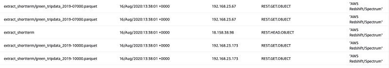
View data shares that are shared from the producer cluster:
```
SELECT * FROM SVV_DATASHARES;
```

The following screenshot shows the output.

You can also see the data shares and their detailed objects and consumers using the following commands:

SHOW DATASHARES;
DESC DATASHARE salesshare;
select * from SVV_DATASHARE_OBJECTS;
select * from SVV_DATASHARE_CONSUMERS;

Viewing and querying data shares for the pool model from the consumer cluster

To view and query data shares from the consumer cluster, complete the following steps:

/**********************************************************/
/* Login to Consumer cluster as awsuser:                  */
/* View datashares and create local database for querying */
/**********************************************************/
select * from SVV_DATASHARE_OBJECTS;

The following screenshot shows the results.

Create a new database from the data share of the producer cluster:

/**********************************************************/
/* Create a local database and schema reference           */
/**********************************************************/
CREATE DATABASE sales_db FROM DATASHARE salesshare
OF NAMESPACE '<producercluster_namespace>';

Optionally, you can create an external schema in the consumer cluster pointing to the schema in the database of the producer cluster.

Creating a local external schema in the consumer cluster allows schema-level access controls within the consumer cluster, and uses a two-part notation when referencing shared data objects (localschema.table; vs. external_db.producerschema.table). See the following code:

/*********************************************************/
/* Create External Schema - Optional                     */
/* reason for schema: give specific access to schema     */
/* using shared alias get access to a secondary database */
/*********************************************************/
CREATE EXTERNAL SCHEMA sales_schema 
FROM REDSHIFT DATABASE 'sales_db' SCHEMA 'sales';

Now you can query the shared data from the producer cluster by using the syntax tenant.schema.table:
```
select * from sales_db.sales.customer;
select * from sales_db.sales.v_customersales;
```

From the tenant1 consumer cluster, you can view the databases and the tenants that are accessible to tenant1. tenant1_schema is as follows:
```
select * from SVV_REDSHIFT_DATABASES;
```

The following screenshot shows the results.

Creating local consumer users and controlling access

You can control access to users in your consumer cluster by creating users and groups, and assigning access to the data share objects.

Log in as an admin user on consumer cluster 1 and enter the following code to create tenant1_group, grant usage on the local database sales_db and schema sales_schema to the group, and assign the user tenant1_user to the tenant1_group:

/********************************************************/
/* Consumers can create own users and assign privileges */
/* Create tenant1_group and assign privileges to read   */
/* sales_db and the sales_schema                        */
/* Create tenant1_user in tenant1_group                 */
/********************************************************/
create group tenant1_group;
create user tenant1_user password 'Redshift#123!' in group tenant1_group;

GRANT USAGE ON DATABASE sales_db TO tenant1_group;
GRANT USAGE ON SCHEMA sales_schema TO GROUP tenant1_group;

Now, login as tenant1_user to consumer cluster 1 and select data from the views v_customer and v_customersales:

/*******************************************************/
/* select from view returns only sales records related */
/* to Consumer A namespace                             */
/*******************************************************/
select * from sales_db.sales.v_customer;
select * from sales_db.sales.v_customersales;

You should see only the data relevant to tenant 1 and not the data that is associated with tenant 2.

Create Materialized views to optimize performance

Consumer clusters can have their own database objects which are local to the consumer. You can also create materialized views on the datashare objects and control when to refresh the dataset for your consumers. This provides another level of isolation from the producer cluster, and will ensure the consumer clusters go against their local dataset.

Log in as an admin user on consumer cluster 1 and enter the following code to create a materialized view for customersales. This will create a local view that can be periodically refreshed from the consumer cluster.

/*******************************************************/
/* Create materialized view in consumer cluster        */
/*******************************************************/
create MATERIALIZED view tenant1_sales.mv_customersales as 
select c_tenantid, c_name, c_region, 
	date_part(w, to_date(s_orderdate,'YYYY-MM-DD')) as "week", 
	date_part(mon, to_date(s_orderdate,'YYYY-MM-DD')) as "month", 
	date_part(dow, to_date(s_orderdate,'YYYY-MM-DD')) as "dow",
	date_part(yr, to_date(s_orderdate,'YYYY-MM-DD')) as "year",
	date_part(d, to_date(s_orderdate,'YYYY-MM-DD')) as "dom", 
	t.t_namespace
from sales_db.tenant t, sales_db.customer c, sales_db.sales s
where t.t_tenantid = c.c_tenantid 
and c.c_tenantid = s.s_tenantid 
and c.c_custid = s.s_custid 
and t.t_namespace = current_namespace;

select * from tenant1_sales.mv_customersales top 100;

REFRESH MATERIALIZED VIEW tenant1_sales.mv_customersales;

With the preceding steps, we have demonstrated how you can control access to the tenant data in the same datastore using views. We also reviewed how data shares help efficiently share data between producer and consumer clusters with transaction consistency. We also saw how a local materialized view can be created to further isolate your BI workloads for your customers and provide a consistent, performant user experience. In the next section we will discuss the Bridge model.

Bridge model

In the bridge model, data for each tenant is stored in its own schema in a database and contains a similar set of tables. Data shares are created for each schema and shared with the corresponded consumer. This is an appealing balance between silo and pool model, providing both data isolation and ETL consolidation. With Amazon Redshift, you can create up to 9,900 schemas. For more information, see Quotas and limits in Amazon Redshift.

With data sharing, separate consumer clusters can be provisioned to use the same managed storage from producer cluster. Consumer clusters have all the capabilities of a producer cluster, and can in turn be producer clusters for data objects they own. Consumers can’t share data that is already shared with them. Without data sharing, queries from all customers are directed to a single cluster. The following diagram illustrates the bridge model.

The following diagram illustrates the bridge model.

To create a multi-tenant architecture using bridge model, complete the steps in the following sections.

Creating database schemas and tables for the bridge model in the producer cluster

As we did in the pool model, the first step is to create the database schema and tables. We log in to the producer cluster as an admin user and create separate schemas for each tenant. For our post, we create two schemas, tenant1 and tenant2, to store data for two tenants.

Use the script below to create two schemas, tenant1 and tenant2, and create tables for customer dimension and sales facts under each of the two schemas. See the following code:

/****************************************/
/* Bridge -  Data Model */
/****************************************/
-- Create schemas tenant1 and tenant2
create schema tenant1;
create schema tenant2;

-- Create tables for tenant1
CREATE TABLE IF NOT EXISTS tenant1.customer (
  c_custid int8 not null ,
  c_name varchar(25) not null,
  c_region varchar(40) not null,
  Primary Key(c_custid)
) diststyle ALL sortkey(c_custid);

CREATE TABLE IF NOT EXISTS tenant1.sales (
  s_orderid int8 not null,
  s_custid int8 not null,
  s_totalprice numeric(12,2) not null,
  s_orderdate date not null,
  Primary Key(s_orderid)
) distkey(s_orderid) sortkey(s_orderdate, s_orderid) ;

  

-- Create tables for tenant2
CREATE TABLE IF NOT EXISTS tenant2.customer (
  c_custid int8 not null ,
  c_name varchar(25) not null,
  c_region varchar(40) not null,
  Primary Key(c_custid)
) diststyle ALL sortkey(c_custid);

CREATE TABLE IF NOT EXISTS tenant2.sales (
  s_orderid int8 not null,
  s_custid int8 not null,
  s_totalprice numeric(12,2) not null,
  s_orderdate date not null,
  Primary Key(s_orderid)
) distkey(s_orderid) sortkey(s_orderdate, s_orderid) ;

Ingest data into the customer dimension and sales fact tables. Using the COPY command is the recommended way to ingest data into Amazon Redshift, but for illustration purposes, we use the INSERT statement:

-- ingest data for tenant1
-- ingest customer data
insert into tenant1.customer values
(1, 'Customer 1', 'NorthEast'),
(2, 'Customer 2', 'SouthEast');

-- ingest sales data
insert into tenant1.sales values
(1, 1, 2434.33, '2020-11-21'),
(2, 2, 54.90, '2020-5-5'),
(3, 2, 9678.99, '2020-3-8');

select count(*) from tenant1.customer;
select count(*) from tenant1.sales;


-- ingest data for tenant2
-- ingest customer data
insert into tenant2.customer values
(1, 'Customer 3', 'NorthWest'),
(2, 'Customer 4', 'SouthEast');

-- ingest sales data
truncate table tenant2.sales;
insert into tenant2.sales values
(1, 2, 452.24, '2020-1-23'),
(2, 1, 76523.10, '2020-11-3'),
(3, 1, 6745.20, '2020-10-01');


select count(*) from tenant2.customer;
select count(*) from tenant2.sales;

Creating data shares and granting usage to the consumer cluster

In the following code, we create two data shares, tenant1share and tenant2share, to share the database objects under the two schemas to the respective consumer clusters.

Create two datashares tenant1share and tenant2share to share the database objects under the two schemas to the respective consumer clusters.

/******************************************************************/
/*   Create Datashare and add database objects to the datashare   */
/******************************************************************/
CREATE DATASHARE tenant1share;
CREATE DATASHARE tenant2share;

Alter the datashare and add the schema(s) for respective tenants to be shared with the consumer cluster
```
ALTER DATASHARE tenant1share ADD SCHEMA tenant1;
ALTER DATASHARE tenant2share ADD SCHEMA tenant2;
```

Alter the datashare and add all tables in the schema(s) to be shared with the consumer cluster

ALTER DATASHARE tenant1share ADD ALL TABLES IN SCHEMA tenant1;
ALTER DATASHARE tenant2share ADD ALL TABLES IN SCHEMA tenant2;

Getting the namespace of the first consumer cluster

Log in to the consumer cluster and get the namespace from the console or by running the select current_namespace command:

/* Grant access to tenant1 schema for Tenant1 BI Cluster */
/* login to tenant1 BI Cluster and get the Namespace 
 * or get the Namespace from the Redshift console */
SELECT CURRENT_NAMESPACE;

Grant usage on the data share for the first tenant to the namespace of the BI cluster. You can get the namespace of the BI cluster from the console or using the SELECT CURRENT_NAMESPACE statement in the BI cluster:

-- Grant usage on the datashare to the first consumer cluster
-- Namespace refers to the namespace GUID of the consumer cluster 
GRANT USAGE ON DATASHARE tenant1share TO NAMESPACE '<consumercluster1_namespace>'
--Account numbers are 12 digit long (optional)
--GRANT USAGE ON DATASHARE tenant1share TO ACCOUNT '<Consumer_AWSAccount>';

Getting the namespace of the second consumer cluster

Log in to the second consumer cluster and get the namespace from the console or by running the select current_namespace command:

/* Grant access to tenant2 schema for Tenant2 BI Cluster */
/*login to tenant1 BI Cluster and get the Namespace      */
SELECT CURRENT_NAMESPACE;

Grant usage on the data share for the second tenant to the namespace of the second consumer cluster you just got from the previous step:

-- Grant usage on the datashare to the second consumer cluster
GRANT USAGE ON DATASHARE tenant2share TO NAMESPACE '<consumercluster2_namespace>'
--Account numbers are 12 digit long (optional)
--GRANT USAGE ON DATASHARE tenant2share TO ACCOUNT '<Consumer_AWSAccount>';

To view data shares from the producer cluster, enter the following code:

/******************************************************************/
/*   View Datashares created, Datashare objects and consumers     */
/******************************************************************/
select * from SVV_DATASHARES;
select * from SVV_DATASHARE_OBJECTS;
select * from SVV_DATASHARE_CONSUMERS;

The following screenshot shows the commands in the query editor.

The following screenshot shows the query results.

Accessing data using the consumer cluster from the data share

To access data using the consumer cluster, complete the following steps:

View data share objects from the SVV_DATASHARE_OBJECTS system view:

/*****************************************************/
/* Consumer cluster as adminuser
/* List the shares available and review contents for each 
/********************************************************/
-- You can view datashare objects associated with the cluster
-- using either of the two commands
SHOW DATASHARES;
select * from SVV_DATASHARES;

The following screenshot shows the query results.

--View objects shared in inbound share for consumer
select * from SVV_DATASHARE_OBJECTS;

The following screenshot shows the query results.

--View namespace or clusters granted usage to a datashare
select * from svv_datashare_consumers;

Create a local database in the first consumer cluster, and an external schema to be able to provide controlled access to the specific schema to the consumer clusters:

/*******************************************************/
/* Create a local database and schema reference        */
/* to the share objects                                */
/*******************************************************/
CREATE DATABASE tenant1_db FROM DATASHARE tenant1share
OF NAMESPACE '<producercluster_namespace>';

Query the database tables using the three-part notation db.tenant.table:

select * from tenant1_db.tenant1.customer;
select * from tenant1_db.tenant1.sales;

Optionally, you can create an external schema.

There are two reasons to create an external schema: either to enable two-part notation access to the tables from the consumer cluster, or to provide restricted access to the specific schemas for selected users, when multiple schemas are shared from the producer cluster. See the following code for our external schema:

/* Create External Schema */
CREATE EXTERNAL SCHEMA tenant1_schema FROM REDSHIFT DATABASE 'tenant1_db' SCHEMA 'tenant1';

If you created the local schemas, you can use the following two-part notation to query the database tables:
```
select * from tenant1_schema.customer;
select * from tenant1_schema.sales;
```

You can view the shared databases by querying the SVV_REDSHIFT_DATABASES table:
```
select * from SVV_REDSHIFT_DATABASES;
```

The following screenshot shows the query results.

Creating consumer users for managing access

Still logged in as an admin user to the consumer cluster, you can create other users who have access to the database objects.

Create users and groups, and assign users and object privileges to the groups with the following code:

/*******************************************************/
/* Consumer can create own users and assign privileges */
/* Create tenant1_user and assign privileges to        */
/* read datashare from tenant1 schema                  */
/*******************************************************/
create group tenant1_group;
create user tenant1_user password 'Redshift#123!' in group tenant1_group;

GRANT USAGE ON DATABASE tenant1_db TO tenant1_user;
GRANT USAGE ON SCHEMA tenant1_schema TO GROUP tenant1_group;

Now tenant1_user can log in and query the shared tables from tenant schema.

/************************************************************/
/* Consumer cluster as tenant1_user - As a consumer cluster */
/* administrator, you must follow these steps:              */
/************************************************************/

select * from tenant1_db.tenant1.customer;
select * from tenant1_db.tenant1.sales;


/************************************************************/
/* If you have created and External Schema                  */
/* you can use the two-part notation to query tables.       */
/************************************************************/

select * from tenant1_schema.customer;
select * from tenant1_schema.sales;

Revoking access to a data share (optional)

At any point, if you want to revoke access to the data share, you can the REVOKE USAGE command:

/*************************************************************/
/* To revoke access at any time use the REVOKE USAGE command */
/*************************************************************/
--Namespace refers to the namespace GUID of the consumer cluster in the account
REVOKE USAGE ON DATASHARE Salesshare FROM NAMESPACE '<consumercluster1_namespace>'
--Account numbers are 12 digit long
REVOKE USAGE ON DATASHARE Salesshare FROM ACCOUNT '<Consumer_AWSAccount>';

Silo model

The third option is to store data for each tenant in separate databases within a cluster. If you need your data isolated from other tenants, you can use the silo model and each database may have distinct data models, monitoring, management, and security footprints.

Amazon Redshift supports cross-database queries across databases, which allow you to simplify data organization. You can store common or granular datasets used across all tenants in a centralized database, and use the cross-database query capability to join relevant data for each tenant.

The steps to create a data share in a silo model is similar to a bridge model; however, unlike a bridge model (where data share is for each schema), the silo model has a data share created for each database. The following diagram illustrates the architecture of the silo model.

The following diagram illustrates the architecture of the silo model.

Creating data shares for the silo model in the producer cluster

To create data shares for the silo model in the producer cluster, complete the following steps:

/*****************************************************/
/** Silo Model – Create databases for the 2 tenants **/
/*****************************************************/
create database tenant1_silodb;

create database tenant2_silodb;

Log in again to the producer cluster with the database name and user ID for the database that you want to share (tenant1_silodb) and create the schema and tables:

/***********************************************************/
/* login to tenant1_db and create schema tenant1 and tables*/
/***********************************************************/
create schema tenant1_siloschema;

-- Create tables for tenant1
CREATE TABLE IF NOT EXISTS tenant1_silodb.tenant1_siloschema.customer (
  c_custid int8 not null ,
  c_name varchar(25) not null,
  c_region varchar(40) not null,
  Primary Key(c_custid)
) diststyle ALL sortkey(c_custid);

CREATE TABLE IF NOT EXISTS tenant1_silodb.tenant1_siloschema.sales (
  s_orderid int8 not null,
  s_custid int8 not null,
  s_totalprice numeric(12,2) not null,
  s_orderdate date not null,
  Primary Key(s_orderid)
) distkey(s_orderid) sortkey(s_orderdate, s_orderid) ;

insert into tenant1_siloschema.customer values
(1, 'Customer 1', 'NorthEast'),
(2, 'Customer 2', 'SouthEast');

truncate table tenant1_siloschema.sales;
insert into tenant1.sales values
(1, 1, 2434.33, '2020-11-21'),
(2, 2, 54.90, '2020-5-5'),
(3, 2, 9678.99, '2020-3-8');

Create a data share with a name for the first tenant (for example, tenant1dbshare):

/******************************************************************/
/*   Create datashare and add database objects to the datashare   */
/******************************************************************/
CREATE DATASHARE tenant1_silodbshare;

Run Alter datashare commands to add the schemas to be shared with the consumer cluster and add all tables in the schemas to be shared with the consumer cluster:
```
ALTER DATASHARE tenant1_silodbshare ADD SCHEMA tenant1_siloschema;
ALTER DATASHARE tenant1_silodbshare ADD ALL TABLES IN SCHEMA tenant1_siloschema;
```

Grant usage on the data share for first tenant to the namespace of the BI cluster. You can get the namespace of the BI cluster from the console or using the SELECT CURRENT_NAMESPACE statement in the BI cluster:

--Namespace refers to the namespace GUID of the consumer cluster in the account
GRANT USAGE ON DATASHARE tenant1_silodbshare TO NAMESPACE ‘<consumercluster1_namespace>’
--Account numbers are 12 digit long (optional)
--GRANT USAGE ON DATASHARE tenant1_silodbshare TO ACCOUNT '<AWS-Account>';

Viewing and querying data shares for the silo model from the consumer cluster

To view and query your data shares, complete the following steps:

Create a new database from the data share of the producer cluster:

CREATE DATABASE tenant1_silodb FROM DATASHARE tenant1_silodbshare
OF NAMESPACE ‘<producercluster_namespace>’;

Now you can start querying the shared data from the producer cluster by using the syntax – tenant.schema.table. If you created an external schema, then you can also use the two-part notation to query the tables.

Query the data with the following code:

select * from tenant1_silodb.tenant1.customer;
select * from tenant1_silodb.tenant1.sales;

Optionally, you can create an external schema pointing to the schema in the database of the producer cluster. This allows you query shared tables using a two-part notation. See the following code:

CREATE EXTERNAL SCHEMA tenant1_siloschema FROM REDSHIFT DATABASE 'tenant1_silodb' SCHEMA 'tenant1';

--With this Schema, you can access using two-part notation to select from data share tables
select * from tenant1_siloschema.customer;
select * from tenant1_siloschema.sales;

You can repeat the same steps for tenant2 to share the tenant2 database with tenant2 You can also control access to users in your consumer cluster by creating users and groups, and assigning access to the data share objects.

System views to view data shares

We have introduced new system tables and views to easily identify the data shares and related objects. You can use three different groups of system views to view the data share objects:

Views starting with SVV_DATASHARES – has detail of datashares and objects in a datashare.

View Name	Purpose
SVV_DATASHARES	View a list of data shares created on the cluster and data shares shared with the cluster
SVV_DATASHARE_OBJECTS	View a list of objects in all data shares created on the cluster or shared with the cluster
SVV_DATASHARE_CONSUMERS	View a list of consumers for data share created on the cluster

Views starting with SVV_REDSHIFT – contains details on both local and remote Redshift databases.

View Name	Purpose
SVV_REDSHIFT_DATABASES	List of all databases that a user has access to
SVV_REDSHIFT_SCHEMAS	List of all schemas that user has access to
SVV_REDSHIFT_TABLES	List of all tables that a user has access to
SVV_REDSHIFT_COLUMNS	List of all columns that a user has access to
SVV_REDSHIFT_FUNCTIONS	List of all functions that user has access to

Views starting with SVV_ALL– contain local and remote databases, external schemas including spectrum and federated query, and external schema references to shared data. If you create external schemas in consumer cluster, you need to use the SVV_ALL views to look at the objects.

View Name	Purpose
SVV_ ALL _SCHEMAS	Union of list of all schemas from SVV_REDSHIFT_SCHEMA view and consolidated list of all external tables and schemas that user has access to
SVV_ ALL _TABLES	List of all tables that a user has access to
SVV_ ALL _COLUMNS	List of all columns that a user has access to
SVV_ ALL _FUNCTIONS	List of all functions that user has access to

Considerations for choosing a storage strategy

You can adopt a storage strategy or choose a hybrid approach based on business, technical, and operational requirements. Before deciding on a strategy, consider the quotas and limits for various objects in Amazon Redshift, and the number of databases per cluster or number of schemas per database to check if it meets your requirements. The following table summarizes these considerations.

	Pool	Bridge	Silo
Separation of tenant data	Views	Schema	Database
ETL pipeline complexity	Low	Low	Medium
Limits	100,000 tables (RA3 – 4x, 16x large clusters)	9,900 schemas per database	60 databases per cluster
Chargeback to consumer accounts	Yes	Yes	Yes
Scalability	High	High	High

Conclusion

In this post, we discussed how you can use the new data sharing feature of Amazon Redshift to implement an AaaS solution with a multi-tenant architecture while meeting SLAs for consumers using separate Amazon Redshift clusters. We demonstrated three types of models providing various levels of isolation for the tenant data. We compared and contrasted the models and provided guidance on when to choose an implementation model. We encourage you to try the data sharing feature to build your AaaS or software as a service (SaaS) solutions.

About the Authors

Rajesh Francis is a Sr. Analytics Specialist Solutions Architect at AWS. He specializes in Amazon Redshift and works with customers to build scalable Analytic solutions.

Neeraja Rentachintala is a Principal Product Manager with Amazon Redshift. Neeraja is a seasoned Product Management and GTM leader, bringing over 20 years of experience in product vision, strategy and leadership roles in data products and platforms. Neeraja delivered products in analytics, databases, data Integration, application integration, AI/Machine Learning, large scale distributed systems across On-Premise and Cloud, serving Fortune 500 companies as part of ventures including MapR (acquired by HPE), Microsoft SQL Server, Oracle, Informatica and Expedia.com.

Jeetesh Srivastva is a Sr. Analytics specialist solutions architect at AWS. He specializes in Amazon Redshift and works with customers to implement scalable solutions leveraging Redshift and other AWS Analytic services. He has worked to deliver on premises and cloud based analytic solutions for customers in banking & finance and hospitality industry verticals.

Querying a Vertica data source in Amazon Athena using the Athena Federated Query SDK

2021-02-11 Kelly Ragan

Post Syndicated from Kelly Ragan original https://aws.amazon.com/blogs/big-data/querying-a-vertica-data-source-in-amazon-athena-using-the-athena-federated-query-sdk/

The ability to query data and perform ad hoc analysis across multiple platforms and data stores with a single tool brings immense value to the big data analytical arena. As organizations build out data lakes with increasing volumes of data, there is a growing need to combine that data with large amounts of data in other data stores. As the variety of data increases, it becomes paramount to have a query tool to bridge two or more data stores with a single query.

Even though data lakes became popular for analytic workloads recently, it’s not uncommon to have data warehouses in addition to data lakes for various reporting and business intelligence (BI) use cases. It becomes imperative to be able to seamlessly query the data stored in the data warehouse and the data lake. To address this issue, Amazon Athena has released a feature called Athena Federated Query. Athena is an interactive query service provided by AWS that makes it easy to analyze data in Amazon Simple Storage Service (Amazon S3) using standard SQL. Vertica is a columnar MPP database platform that can be deployed in the cloud or on premises, and supports exabyte scale data warehouses. With Athena Federated Query and the Vertica connector, you can now run analytical queries over a data warehouse on Vertica and a data lake in Amazon S3.

Athena Federated Query includes pre-built connectors to a variety of AWS services and databases, as well as an SDK to build custom connectors to other databases and data stores. With this feature, federated queries can pull data from a data lake in an S3 bucket and from an external data source, and then combine it into a single result set in Athena. These connectors are an extension of the Athena query engine, which translates content between Athena and the external data source. Pre-built connectors exist for Amazon CloudWatch Logs, Amazon DynamoDB, Amazon DocumentDB (with MongoDB compatibility), and Amazon Relational Database Service (Amazon RDS), as well as a JDBC connector for Amazon Redshift, MySQL, and PostgreSQL. For other types of relational databases, you can use the Athena Federated Query SDK to create a custom connector.

In this post, we demonstrate how to deploy the custom connector between Athena and a Vertica database built using the Athena Federated Query SDK. After deploying the custom connector, we demonstrate issuing federated queries and moving data from Vertica to a data lake using CREATE TABLE AS (CTAS) with a federated query.

AWS services used in the solution

The Athena Federated Query SDK is an open-source framework to build custom connectors, and comes with a connector publish tool that deploys the connector executables in an application to the AWS Serverless Application Repository. The Athena Federated Query uses an AWS Lambda function that in turn uses the application deployed to the AWS Serverless Application Repository.

A custom connector is composed of a Lambda function that utilizes three components:

MetadataHandler – An interface that exposes metadata information of schemas, tables, and columns from the underlying data store to Athena
RecordHandler – An interface that provides hooks to read data from the external source and share it with the Athena query engine in Apache Arrow columnar format
CompositeHandler – For managing running the MetadataHandler and RecordHandler

The Lambda function connects to the external data store using an appropriate connection protocol and sends the parsed SQL statement. In the case of Vertica, it is JDBC. The RecordHandler processes the result set produced by the external data store and passes the rows to Athena for final processing. Multiple Lambda functions are called by Athena depending on the Lambda concurrency settings to read the result set in parallel. A spill bucket is used to handle a large dataset that exceeds the Lambda server’s capacity to process the result set.

The JDBC connection established by the Lambda function to the external database is used to send the parsed SQL statement and retrieve the result set rows from the external database. This scenario works well in terms of bandwidth for smaller databases and result sets. However, you might have Vertica deployments with petabyte or exabyte data warehouses. Typical queries return result sets on the order of 10, 20, 30 gigabytes, or more. Due to the bandwidth issue with a JDBC connection, the solution presented in this post modifies the Athena Federated Query SDK to implement a different route for the transmission of large result sets from Vertica to the Athena server for final processing.

The alternate solution utilizes the Vertica EXPORT command as a wrapper around the parsed SQL statement. You can use the EXPORT command to write a result set for a SQL statement directly to an S3 bucket using Vertica’s highly parallelized write to Amazon S3 using partitioning. This solution modifies the SDK to allow Athena to read the result set in the S3 bucket, determine the number of partitions, and call subsequent Lambda functions to parallelize the read of the result set. This produces an efficient way to move a multi-gigabyte result set from Vertica to Athena with parallelized writes from Vertica to Amazon S3 and parallelized reads from Amazon S3 to Athena. When connecting to the Vertica database, the SDK uses AWS Secrets Manager to retrieve a user ID and password for a service account on the Vertica database.

Solution architecture

The following diagram shows the solution architecture for the Vertica custom connector when deployed to AWS.

The connector components are as follows:

A user issues a federated SQL query in Athena against a table in Vertica.
Athena parses the query and calls a Lambda function.
The Lambda function makes a call to Secrets Manager to get the user ID and password for connecting to Vertica.

The connector sends an EXPORT statement wrapper with the embedded SQL statement to Vertica through the JDBC connection. For example, see the following code:

EXPORT TO PARQUET (directory = 's3://<bucket_name>/<folder_name>, 
Compression='Snappy', fileSizeMB=64) OVER() as   
SELECT  
ORDER_ID,  
ITEM,  
CUSTOMER_ID,
ORDERED_DATE
FROM SCHEMA1.ORDERS  
WHERE CUSTOMER_ID = 2;

Vertica processes the SQL query and writes the result set to the S3 bucket specified in the EXPORT command. Vertica parallelizes the write to S3 bucket based on the fileSizeMB parameter into as many partitions as needed for the result set.
Athena calls a Lambda function to scan the S3 bucket in order to determine the number of files to read for the result set.
Athena invokes multiple Lambda functions depending on the number of partitions using Amazon S3 Select. This allows Athena to parallelize the read of the S3 files.
Athena combines the result set returned from Vertica with data scanned from the data lake, and returns the combined result set to the user.

Prerequisites

Before you get started, make sure you have the following prerequisites:

Amazon EC2 IAM role permissions – The AWS Identity and Access Management (IAM) role of the Amazon Elastic Compute Cloud (Amazon EC2) machines hosting the Vertica database must be given write permissions to the VerticaExport S3 bucket, which is created when deploying the connector.
Secrets Manager – The Vertica connection credentials are stored in Secrets Manager. The secret name is prefixed with Vertica– and the secret value is the connection credentials.
Lambda IAM role permissions – When the Lambda function is deployed to the AWS Serverless Application Repository, it creates a custom IAM role for the function to run. The custom role has the following IAM permissions in order to successfully perform the read and write functions associated with the MetadataHandler and RecordHandler:
- AWSLambdaBasicExecutionRole
- AWSLambdaVPCAccessExecutionRole
- For Secrets Manager, GetSecretValue for secrets with a prefix given in SecretNameOrPrefix
- For Amazon S3, list, read, and write permissions for SpillBucket and ExportBucket, and list permissions for all S3 buckets
- For Athena, GetQueryExecution

Demonstration tables

To demonstrate the Athena Vertica connector capabilities, we use the following components:

A Vertica database running in our AWS environment.
A Vertica table called orders containing details of customer orders.
An Athena table called customer, which has an S3 bucket as a data source. This table contains information regarding customers.

The following screenshot shows the details of the customer table in Amazon S3.

The following screenshot shows the details of the customer table in Amazon S3.

The following screenshot shows the details of the orders table in Vertica.

The following screenshot shows the details of the orders table in Vertica.

Setting up the Athena Vertica connector project

To set up your connector project, complete the following steps:

Create an S3 bucket in your AWS account. This is the bucket where the result set from Vertica is exported.
Create another S3 bucket in your AWS account. This is the bucket where the code for the connector is stored and retrieved.
Grant the IAM role of the EC2 machines hosting the Vertica database read and write permissions to the S3 result set bucket, allowing Vertica to export data to the bucket.
Clone the GitHub repo in your local folder.
Open the project in your preferred IDE.
From the athena-query-federation directory, run mvn clean install.
From the athena-vertica directory, run mvn clean install.
From the athena-vertica directory, run ../tools/publish.sh <s3_code_bucket_name> athena-vertica [region] to publish the connector to your private AWS Serverless Application Repository.
Upon successful completion of the script, the connector’s serverless application is published to the AWS Serverless Application Repository.

Deploying the connector

To deploy your connector, complete the following steps:

On the AWS Serverless Application Repository console, choose Published Applications.
On the Private Applications tab, select Show apps that create in order to see deployed applications.
Choose the VerticaAthenaConnector serverless app.
For AthenaCatalogName, enter the name of the connector Lambda function used when querying the Vertica tables (avc).
For SecretNameOrPrefix, enter the prefix used to store the Vertica credentials in Secrets Manager (the default is Vertica-).
For SpillBucket, enter the S3 bucket name where data is spilled in case the result set data volume crosses a certain limit (test-spill-bucket).
For VerticaExportBucket, enter the S3 bucket where the result set from Vertica is exported (test-export-bucket).
For VpcId, enter your VPC ID.

For VpcId, enter your VPC ID.

For SpillPrefix, enter athena-spill.
For SubnetIds, enter your subnet IDs.
For VerticaConnectionString, enter the connection string of the Vertica database in the following format:
```
jdbc:vertica://<host_name>:<port>/<database>?user=${vertica-username}&password=${vertica-password}
```
Where, vertica-username and vertica-password are the secret names of the Vertica user credentials stored in AWS Secrets Manager.

Select I acknowledge that this app creates custom IAM roles.

Select I acknowledge that this app creates custom IAM roles.

Choose Deploy.

Upon successful deployment, a Lambda function with the name given for AthenaCatalogName is deployed in your AWS environment. We use this function to issue federated queries to Vertica. The connector is now deployed and ready to use.

Using the connector

On the Athena console, you can query Vertica tables as shown in the following code. The value for <lambda_function> corresponds to the function you created in the previous section.

SELECT  
ORDER_ID,   
CUSTOMER_ID,
PRODUCT_ID,
PRODUCT_NAME,
ORDER_DATE
FROM "lambda:<lambda_function>".SCHEMA1.ORDERS  
WHERE CUSTOMER_ID <= 3461
ORDER BY ORDER_ID DESC

In this example, we named the function as avc. The following screenshot shows our query results.

The following screenshot shows our query results.

This demonstrates that the newly deployed connector read the user-requested columns and the Vertica source table, wrapped an EXPORT statement around the SQL statement, and ran it in Vertica. The results of this query were exported to the specified S3 bucket (test-export-bucket) in Parquet format. The connector then invoked multiple Lambda functions to read the data from the S3 bucket using Amazon S3 Select and displayed it on the Athena console. Note that currently the connector exports Vertica timestamp and timestamptz data types as a varchar data type. Therefore we need to use the date_parse(string, format) function to convert the timestamps columns into the correct data type.

We can also create an Athena table using CTAS with the result set of the Vertica query using the following query:

CREATE TABLE default.vertica_customers_table AS (
SELECT  
ORDER_ID,
CUSTOMER_ID,
PRODUCT_ID,
PRODUCT_NAME,
ORDER_DATE
FROM "lambda:<lambda_function>".SCHEMA1.ORDERS  
WHERE CUSTOMER_ID <= 3461
);

We can then use the newly created table to query the data as shown in the following screenshot.

In addition, we can also query and join the customer data in Amazon S3 and orders data in Vertica using the following sample query:

WITH   
customer_data AS (  
  SELECT   
   	CUSTOMER_NAME,  
   	CUSTOMER_ID  
    
  FROM default.customer
  ),  
orders_data AS (  
  SELECT    
   	ORDER_ID,  
   	PRODUCT_NAME,  
   	CUSTOMER_ID   
  FROM "lambda:<lambda_function>".schema1.orders  
  )  
SELECT a.CUSTOMER_ID, b.ORDER_ID, b.PRODUCT_NAME
FROM customer_data a 
INNER JOIN orders_data b
ON a.customer_data.customer_id = b.orders_data.customer_id 
WHERE lower(b.PRODUCT_NAME) like 'pencil'
ORDER BY b.ORDER_ID DESC

This query joins the orders data in Vertica with customer data in the S3 bucket in the customer_id column and displays the results on the Athena console.

This query joins the orders data in Vertica with customer data in the S3 bucket in the customer_id column and displays the results on the Athena console.

This demonstrates the ease of performing analytics across multiple platforms and data stores.

Conclusion

In this post, we introduced the Athena Vertica connector, its solution architecture, and demonstrated how to deploy the connector using the Athena Federated Query SDK. We saw how to run SQL queries on the Vertica data source. We also learned that we can use the connector to perform extract, transform, and load operations on the data in the Vertica tables and Amazon S3, enabling us to perform faster and better analytics across multiple platforms and data sources.

For more information about Athena Federated Query, see the GitHub repo.

Special Acknowledgement

Special acknowledgement goes to the Intuit Data Engineering staff Denise McInerney – Data Architect, Sanjay Rane – Group Engineering Manager – Data, and Kannan Nagarajan – Database Architect. They helped design, review, and support the development of the custom connector and architecture.

About the Authors

Kelly Ragan is a Senior Data Architect, Strategic Accounts Team, AWS Professional Services. He helps customers solve big data problems and wrestle with large-scale data warehouses. In his spare time, he enjoys snow skiing, bicycling, and camping in the Pacific Northwest.

Rohit Masur is an Associate Big Data Consultant, Data and Analytics Team, AWS Professional Services. He helps customers architect and implement solutions on AWS to get business value out of data. In his spare time, he enjoys reading books, going on long walks, and exploring new hiking trails in the Bay Area.

Automating AWS service logs table creation and querying them with Amazon Athena

2021-02-05 Michael Hamilton

Post Syndicated from Michael Hamilton original https://aws.amazon.com/blogs/big-data/automating-aws-service-logs-table-creation-and-querying-them-with-amazon-athena/

I was working with a customer who was just getting started using AWS, and they wanted to understand how to query their AWS service logs that were being delivered to Amazon Simple Storage Service (Amazon S3). I introduced them to Amazon Athena, a serverless, interactive query service that allows you to easily analyze data in Amazon S3 and other sources. Together, we used Athena to query service logs, and were able to create tables for AWS CloudTrail logs, Amazon S3 access logs, and VPC flow logs. As I was walking the customer through the documentation and creating tables and partitions for each service log in Athena, I thought there had to be an easier and faster way to allow customers to query their logs in Amazon S3, which is the focus of this post.

This post demonstrates how to use AWS CloudFormation to automatically create AWS service log tables, partitions, and example queries in Athena. We also use the SQL query editor in Athena to query the AWS service log tables that AWS CloudFormation created.

Athena best practices

This solution is appropriate for ad hoc use and queries the raw log files. These raw files can range from compressed JSON to uncompressed text formats, depending on how they were configured to be sent to Amazon S3. If you need to query over hundreds of GBs or TBs of data per day in Amazon S3, performing ETL on your raw files and transforming them to a columnar file format like Apache Parquet can lead to increased performance and cost savings. You can save on your Amazon S3 storage costs by using snappy compression for Parquet files stored in Amazon S3. To learn more about Athena best practices, see Top 10 Performance Tuning Tips for Amazon Athena.

Table partition strategies

There are a few important considerations when deciding how to define your table partitions. Mainly you should ask: what types of queries will I be writing against my data in Amazon S3? Do I only need to query data for that day and for a single account, or do I need to query across months of data and multiple accounts? In this post, we talk about how to query across a single, partitioned account.

By partitioning data, you can restrict the amount of data scanned per query, thereby improving performance and reducing cost. When creating a table schema in Athena, you set the location of where the files reside in Amazon S3, and you can also define how the table is partitioned. The location is a bucket path that leads to the desired files. If you query a partitioned table and specify the partition in the WHERE clause, Athena scans the data only for that partition. For more information, see Table Location in Amazon S3 and Partitioning Data. You can then define partitions in Athena that map to the data residing in Amazon S3.

Let’s look at an example to see how defining a location and partitioning our table can improve performance and reduce costs. In the following tree diagram, we’ve outlined what the bucket path may look like as logs are delivered to your S3 bucket, starting from the bucket name and going all the way down to the day.

In the following tree diagram, we’ve outlined what the bucket path may look like as logs are delivered to your S3 bucket

Outlined in red is where we set the location for our table schema, and Athena then scans everything after the CloudTrail folder. We then outlined our partitions in blue. This is where we can specify the granularity of our queries. In this case, we partition our table down to the day, which is very granular because we can tell Athena exactly where to look for our data. This is also the most performant and cost-effective option because it results in scanning only the required data and nothing else.

If you have to query multiple accounts and Regions, you should back off the location to AWSLogs and then create a non-partitioned CloudTrail table. This allows you to write queries across all your accounts and Regions, but the trade-off is that your queries take much longer and are more expensive due to Athena having to scan all the data that comes after AWSLogs every query. However, querying multiple accounts is beyond the scope of this post.

Prerequisites

Before you get started, you should have the following prerequisites:

Service logs already being delivered to Amazon S3
An AWS account with access to your service logs

Deploying the automated solution in your AWS account

The following steps walk you through deploying a CloudFormation template that creates saved queries for you to run (Create Table, Create Partition, and example queries for each service log).

Choose Launch Stack:

Choose Next.
For Stack name, enter a name for your stack.

You don’t need to have every AWS service log that the template asks for. If you don’t have CloudFront logs for example, you can leave the PathParameter as is. If you need CloudFront logs in the future, you can simply update the Create Table statement with the correct Amazon S3 location in Athena.

For each service log table you want to create, follow the steps below:

Replace <_BUCKET_NAME> with the name of your S3 bucket that holds each AWS service log. You can use the same bucket name if it’s used to hold more than one type of service log.
Replace <Prefix> with your own folder prefix in Amazon S3. If you don’t have a prefix, make sure to remove it from the path parameters.
Replace <ACCOUNT-ID> and <REGION> with desired account and region.

Choose Next.

Choose Next.
Enter any tags you wish to assign to the stack.
Choose Next.
Verify parameters are correct and choose Create stack at the bottom.

Verify the stack has been created successfully. The stack takes about 1 minute to create the resources.

Querying your tables

You’re now ready to start querying your service logs.

On the Athena console, on the Saved queries tab, search for the service log you want to interact with.

On the Athena console, on the Saved queries tab, search for the service log you want to interact with.

Choose Create Table – CloudTrail Logs to run the SQL statement in the Athena query editor.

Make sure the location for Amazon S3 is correct in your SQL statement and verify you have the correct database selected.

Choose Run query or press Tab+Enter to run the query.

Choose Run query or press Tab+Enter to run the query.

The table cloudtrail_logs is created in the selected database. You can repeat this process to create other service log tables.

For partitioned tables like cloudtrail_logs, you must add partitions to your table before querying.

On the Saved queries tab, choose Create Partition – CloudTrail.
Update the Region, year, month, and day you want to partition. Choose Run query or press Tab+Enter to run the query.

Choose Run query or press Tab+Enter to run the query.

After you run the query, you have successfully added a partition to your cloudtrail_logs table. Let’s look at some of the example queries we can run now.

On the Saved queries tab, choose Query – CloudTrail Logs.

This is a base template included to begin querying your CloudTrail logs.

Highlight the query and choose Run query.

You can see the base query template uses the WHERE clause to leverage partitions that have been loaded.

Let’s say we have a spike in API calls from AWS Lambda and we want to see the users that the calls were coming from in a specific time range as well as the count for each user. Our query looks like the following code:

SELECT useridentity.sessioncontext.sessionissuer.username as "User",
       count(eventname) as "Lambda API Calls"
FROM cloudtrail_logs
WHERE eventsource = 'lambda.amazonaws.com'
       AND eventtime BETWEEN '2020-11-24T18:00:00Z' AND '2020-11-24T21:00:00Z' 
group by useridentity.sessioncontext.sessionissuer.username
order by count(eventname) desc

Or if we wanted to check our S3 Access Logs to make sure only authorized users are accessing certain prefixes:

SELECT *
FROM s3_access_logs
WHERE key='prefix/images/example.jpg'
        AND requester != 'arn:aws:iam::accountid:user/username'

Cost of solution and cleaning up

Deploying the CloudFormation template doesn’t cost anything. You’re only charged for the amount of data scanned by Athena. Remember to use the best practices we discussed earlier when querying your data in Amazon S3. For more pricing information, see Amazon Athena pricing and Amazon S3 pricing.

To clean up the resources that were created, delete the CloudFormation stack you created earlier. This also deletes the saved queries in Athena.

Summary

In this post, we discussed how we can use AWS CloudFormation to easily create AWS service log tables, partitions, and starter queries in Athena by entering bucket paths as parameters. We used CloudTrail and Amazon S3 access logs as examples, but you can replicate these steps for other service logs that you may need to query by visiting the Saved queries tab in Athena. Feel free to check out the video as well, where I go over how we store logs in Amazon S3 and then give a quick demo on how to deploy the solution.

For more information about service logs, see Easily query AWS service logs using Amazon Athena.

About the Author

Michael Hamilton is a Solutions Architect at Amazon Web Services and is based out of Charlotte, NC. He has a focus in analytics and enjoys helping customers solve their unique use cases. When he’s not working, he loves going hiking with his wife, kids, and a 2-year-old German shepherd.

How Baqend built a real-time web analytics platform using Amazon Kinesis Data Analytics for Apache Flink

2021-02-05 Wolfram Wingerath

Post Syndicated from Wolfram Wingerath original https://aws.amazon.com/blogs/big-data/how-baqend-built-a-real-time-web-analytics-platform-using-amazon-kinesis-data-analytics-for-apache-flink/

This is a customer post written by the engineers from German startup Baqend and the AWS EMEA Prototyping Labs team.

Baqend is one of the fastest-growing software as a service (SaaS) startups in Germany, serving over 5,000 business customers with more than 100 million monthly users and $2 billion EUR revenue per year. Baqend’s main product is a one-click solution to accelerate ecommerce websites called Speed Kit. By rerouting a portion of the web traffic through Speed Kit’s caching infrastructure, it achieves a typical performance boost between 1.5–3 times faster.

To measure the impact of Speed Kit and confirm its uplift to Baqend’s customers, we maintain several dashboards that display the technical and business performance improvements achieved by Speed Kit. This requires complex aggregations of tracking data collected during A/B tests on our customers’ websites.

The Challenge: Real-time analytics and reporting at scale

One of the key issues with our legacy solution for monitoring and reporting needed to process. The raw tracking data from all users was batched through various systems, which resulted in processing delays up to 24 hours for some analytics jobs. This impacted our operations monitoring and sales activities negatively, because our customers sometimes couldn’t analyze the impact of deployment changes until the next day. Furthermore, our legacy reporting service lacked any support for custom visualization development.

This post shows you how we transformed our batch-based analytics process into a continuous complex event-processing pipeline, which is managed by Amazon Kinesis Data Analytics for Apache Flink. The new solution exhibits less than a minute of end-to-end latency from data ingestion to visual output in the dashboard.

The key topics presented in this post are:

Fully managed and highly scalable service architecture – Our architecture is based on fully managed AWS services that made it easy to scale from 1 to over 100 million users
Continuous analytics – We transformed our high-volume batch analytics processes with daily updates into an efficient incremental aggregation process with sub-minute latency based on Kinesis Data Analytics for Apache Flink
Real-time reporting – We connected our aggregation pipeline to a fully customizable dashboard for data exploration based on Amazon Elasticsearch Service (Amazon ES) and Kibana

Solution overview and key components

Following a remote planning phase in which we defined our requirements and laid out the basic design, we built the solution on an on-site prototyping engagement with AWS over the course of 4 weeks in early 2020 in Hamburg. Seven team members from Baqend and AWS EMEA Prototyping Labs implemented the following architecture.

Following a remote planning phase in which we defined our requirements and laid out the basic design.

The workflow includes the following steps:

The performance tracking data is streamed by Speed Kit Amazon Elastic Compute Cloud (Amazon EC2) instances.
This data goes into an Amazon Kinesis Data Streams
This data stream is consumed by a Kinesis Data Analytics for Apache Flink application.
The data is ingested into Amazon ES.
This streaming application relies on AWS Secrets Manager to store and access the credentials for Elasticsearch with basic HTTP authentication.
An Nginx proxy server application hosted on EC2 instances in multiple public subnets and Availability Zones redirects the user requests Kibana with Amazon Cognito authentication (for more information, see How do I use an NGINX proxy to access Kibana from outside a VPC that’s using Amazon Cognito authentication?).
The Apache Flink application also uses Amazon DynamoDB as a backend for long-living external states required for certain operations (covered later in this post).
The streaming application also delivers the raw and intermediate data outputs to an Amazon Simple Storage Service (Amazon S3) bucket to enable historical data analysis and operational troubleshooting with Amazon Athena.

Although the prototyping engagement also covered other aspects, we focus on the Kinesis Data Analytics application in the following sections of this post.

Continuous aggregation with Kinesis Data Analytics

We need to collect all kinds of technical data points on every page load of a website visitor. Details on the individual page impressions (PI) help us analyze web performance for the websites of our customers. Speed Kit provides a performance tracking functionality that collects data within the browser of every website visitor and sends it to our analytics backend.

Aggregating page impressions

Intuitively, there should be only one data beacon for any given PI because the data could be aggregated in the browser before it’s sent to our backend. Speed Kit sends several data beacons during the page load to minimize the possibility of any data loss, as shown in the following figure.

Speed Kit sends several data beacons during the page load to minimize the possibility of any data loss, as shown in the following figure.

For example, static information such as the target URL or the current time can be sent away as soon the navigation starts (navigation beacon), whereas certain measurements can’t be sent until very late in the load process, like the time it took to load the entire page (load beacon). Certain events may even occur minutes after the page load, or not at all (for example, user interaction with the page or JavaScript errors) and are therefore handled via dedicated and optional transmissions (event beacons). These beacons need to be correlated in our analytical backend later on.

Aggregating session data

Because some of the most interesting metrics are computed on the level of user sessions, aggregating all data beacons for the individual PIs isn’t enough to analyze web performance. For instance, the user engagement metrics are often quantified by the number of pages visited in one sitting (session length) or the share of users that left on the very first page (bounce rate).

Aggregating relevant information may even involve identifying and removing duplicates, as illustrated in the following figure.

Suppose the user first checks out the landing page and immediately leaves (Session 1), and then comes back later to browse through some products and buy some blue shoes (Session 2), and finally returns after a few hours to reload the order confirmation page and browse some more products (Session 3). Because Session 3 starts with a reload of the order confirmation page, tracking data on the order that was completed in Session 2 is transmitted a second time, resulting in a potentially duplicated count of the completed orders. Therefore, our analytical backend needs to identify the duplicated tracking information as such and ignore it for further analysis. To enable this, we persistently store a salted hash of every order ID and simply have the aggregation pipeline drop the tracking data on any order that has already been written to the external key value store (see the diagram in the following section).

Anatomy of the streaming application

The following diagram shows our event processing pipeline from raw data collection to the storage of aggregation results.

The workflow is as follows:

The first step is tracking the data within the browsers of the end users.
The data is sent to Kinesis Data Streams for consumption through a custom stateful Apache Flink process function within a Kinesis Data Analytics application.
Raw data beacons are initially normalized and invalid data beacons are delivered to Amazon S3 via side outputs to facilitate later analysis of all data that has been sorted out.
As mentioned earlier, we use a DynamoDB table to run a deduplication rule over all incoming order data (confirmation pages) by the DynamoDB Transactions API. We also use another DynamoDB table to identify bot traffic by storing the user agent strings that have been associated with suspicious behavior consistently (because they belong to web crawlers). Finally, the stream of cleaned tracking beacons is processed in stateful window aggregation steps for storage.
We aggregate all beacons referring to the same PI and write them off to our data lake on Amazon S3 to enable offline analysis with Athena.
Furthermore, we compile the tracking beacon stream into 1-minute summaries containing both PI and session data for storage via Amazon ES to enable efficient reporting with Kibana.

State storage and application management

Most of the application state for the streaming application is held in the built-in RocksDB state backend with incremental checkpointing. This default built-in state storage mechanism depends on a 50 GB storage limit provided for each Kinesis Processing Unit (KPU) allocated to a Kinesis Data Analytics application. On the other hand, we used DynamoDB tables to store the state permanently for unique conversions and user agent strings in order to decouple historical state for these two data types from Apache Flink application management and to keep the checkpointing duration and size under control. Using DynamoDB for these two use cases helps to control the overhead for creating and restoring checkpoints and thereby controls the application startup time.

Workload distribution and scalability

As of February 2021, our processing pipeline handles over 2.8 billion tracking beacons per month, which corresponds to more than 500 million individual PIs from over 140 million user sessions and more than 100 million unique users. Achieving this scale requires even distribution of both processing and storage load across all stream partitions. Therefore, we use randomly generated session IDs as a partitioning key for the input Kinesis data stream and throughout most of the remaining sections of our pipeline.

In the presence of certain anomalies such as heavy bot traffic, a load skew may occur regardless, which may impair overall throughput or even crash the entire application in extreme cases. We monitor the number of incoming and outgoing records (to derive the current buffer size) for the individual Apache Flink operators in every stream partition to identify issues with the load distribution quickly and generate alert notifications via multiple channels (such as Slack and email) if the measurements for different stream partitions diverge significantly. For convenience, we further visualize custom Amazon CloudWatch metrics in a Grafana dashboard.

Event processing, delivery semantics, and fault tolerance

The application restarts and downtime (such as during and after application deployment) can be handled seamlessly by using Apache Flink’s event time processing semantics as generated output is independent of the wall-clock time of the processing nodes. All processing is based on monotonically increasing ingestion timestamps to eliminate the possibility of late arrivers. While our data cleaning procedure identifies the invalid records, it never drops any data items from the stream, but instead it only attaches information on the detected issue to the data item in question. This approach enables us to analyze the frequency and distribution of every problem in our aggregation pipeline by using the same Kibana dashboard.

Even though the data ingestion to Amazon ES provides at-least-once delivery guarantees by default, we managed to achieve exactly-once delivery guarantees from the source Kinesis data stream to the Elasticsearch index by generating document identifiers in a deterministic fashion. Therefore, the data stream can be replayed safely because the existing data records are overwritten on re-insertion into the Elasticsearch index.

Data retention and multi-tenancy in Amazon ES

We store pre-aggregated data at the minute level in Amazon ES to make sure our Kibana dashboard remains responsive even when analyzing a scope of weeks or months. As illustrated in the following figure, the Apache Flink application summarizes the raw tracking data along different dimensions (browser, device, test group, and aggregation time in minutes) before writing it to Elasticsearch.

Apache Flink application summarizes the raw tracking data along different dimensions (browser, device, test group, and aggregation time in minutes) before writing it to Elasticsearch.

The Elasticsearch documents are composed of bucketed histogram data for performance timers such as the First Contentful Paint (FCP) instead of the actual timer values. Running queries over these aggregates instead of the raw data minimizes query run costs significantly: traffic-heavy customers may have tens of millions of raw tracking beacons in a single week, whereas the number of 1-minute buckets is several orders of magnitudes lower (for small and large customers alike). We observe over 5 times more PIs and 30 times more raw beacons than aggregates stored in Elasticsearch across all of our customers.

We store the data for different customers in separate indexes generated for a fixed temporal rolling period by the Apache Flink Elasticsearch Sink Connector. We also implemented customer-specific retention policies in Amazon ES by deleting the old indexes as required. Our deployment is multi-tenant so that our customers can receive fine-grained access only to their own data stored in the indexes created for them.

Kibana for continuous reporting

We used Kibana to build our dashboards because it provides powerful and easy-to-create built-in visualizations and virtually boundless flexibility through custom Vega chart visualizations. Kibana also works well in combination with Elasticsearch indexes, thereby facilitating the role-based access management that enables us to provide individual customers access to the data in our multi-tenant dashboard.

Easy data exploration

The following illustration shows one of the standard visualizations in Kibana that we use to understand the distribution of device types and browsers used by website visitors.

Real-time histogram visualization

Illustrating the distribution of performance metrics requires using a custom visualization. The following custom Vega histogram chart illustrates by the concrete performance metric LCP how Speed Kit improves the webpage load time.

The following custom Vega histogram chart illustrates by the concrete performance metric LCP how Speed Kit improves the webpage load time.

In comparison with the vanilla website where page loads are almost never faster than 2 seconds (pink area), Speed Kit-accelerated end users experience comparatively faster and even sub-second level load times (blue area).

Because our main business revolves around accelerating our customers’ websites, visualizing the actual uplift is critical for all developers (to debug performance and identify issues quickly) as well as our customers (highlighting the value of our product). With the continuous aggregation and reporting solution outlined in this post, we were able to satisfy all these requirements in a scalable and fully managed fashion.

Conclusion and future directions

In this post, we shared our journey from a high-volume batch analytics solution to a continuous aggregation pipeline using Kinesis Data Analytics for Apache Flink. Key aspects are:

End-to-end processing time is reduced from 24 hours to sub-minute latency.
We implemented a fully functional prototype within 4 weeks. The AWS Prototyping team enabled us to build our system on a multitude of managed AWS services.
The system was used with production load after 8 weeks.
The new system based on the Kinesis Data Analytics for Apache Flink application exhibits extreme scalability as it handles workloads with ease that were infeasible for the old system. As of February 2021, our system processes more than 500 million page loads from over 100 million unique users every month.
Elasticsearch and Kibana with customized Vega visualizations provides flexible and continuously updating dashboards for all our customers.

Additional Resources

For more details on the challenges and solutions discussed in this article, we recommend the following resources:

We would be glad to get feedback on our work, so please drop us a line in case of any remaining questions!

About the Authors

Wolfram “Wolle” Wingerath heads the data engineering team that is responsible for developing and operating Baqend’s infrastructure for analytics and reporting.

Florian Bücklers is Baqend’s Chief Technology Officer and therefore responsible for coordinating between the different teams for front-end and backend development, devOps, onboarding, and data engineering.

Benjamin Wollmer develops data-intensive systems at Baqend, but he is also doing his PhD at the University of Hamburg and therefore likes to read and write about related topics.

Stephan Succo is one of the core developers of Baqend’s continuous analytics pipeline.

Jörn Domnik is a Senior Software Engineer at Baqend with a focus on backend development and reliability engineering.

As a DevOps engineer, Virginia Amberg monitors cluster health and keeps all systems running smoothly at Baqend.

As a Principal Prototyping Engagement Manager in AWS, Markus Bestehorn is responsible for building business-critical prototypes with AWS customers and is a specialist for IoT and machine learning.

As a Data Prototyping Architect in AWS, Anil Sener builds prototypes on big data analytics, data streaming, and machine learning, which accelerates the production journey on the AWS Cloud for top EMEA customers.

As B2B Strategic Account Manager for Startups at AWS, Daniel Zäeh works with customers to make their ideas come true and helps them grow, by connecting tech and business.

Building AWS Data Lake visualizations with Amazon Athena and Tableau

2021-02-02 Dhiraj Thakur

Post Syndicated from Dhiraj Thakur original https://aws.amazon.com/blogs/big-data/building-aws-data-lake-visualizations-with-amazon-athena-and-tableau/

Amazon Athena is an interactive query service that makes it easy to analyze data in a data lake using standard SQL. One of the key elements of Athena is that you only pay for the queries you run. This is an attractive feature because there is no hardware to set up, manage, or maintain.

You can query Athena with SQL or by using data visualization tools such as Amazon QuickSight, Tableau, or other third-party options. QuickSight is a cloud-native business intelligence (BI) service that you can use to visually analyze data and share interactive dashboards with all users in your organization. QuickSight is fully managed and serverless, requires no client downloads for dashboard creation, and has a pay-per-session pricing model that allows you to pay for dashboard consumption with a maximum charge of $5.00 per reader per month. The combination of QuickSight and Athena allows you to rapidly deploy dashboards and BI to tens of thousands of users, while only paying for actual usage, and not worrying about server deployment or management. Tableau allows you to similarly share dashboards with readers when utilizing Tableau servers. This post demonstrates how you can connect to Athena from a Tableau desktop, create a dashboard that queries data from Athena, and publish to a Tableau server for broader distribution.

Integration of Tableau with Athena as a data source is gaining in popularity, and many customers prefer to create Tableau dashboards on Athena. Performance of the dashboard usually varies based on many factors, such as number of fields and views, data size, network bandwidth, Athena query runtime, dashboard rendering time, connection type, and location of the Tableau server (on premises or AWS). We walk you through the required configuration to integrate Tableau with Athena, best practices, and Athena runtime analysis.

Solution overview

In this solution, we build an end-to-end Tableau dashboard using Athena as a data source for data analysts. The dashboard has two views:

Student’s study time based on age group and gender
Geo location of the students

The dashboard is very helpful in analyzing a student’s performance in the class and their health condition.

You walk through the following steps:

Configure Tableau to connect to Athena.
Connect Tableau Desktop to Athena to build dashboard.
Create a Tableau dashboard and publish to Tableau server.
Analyze the Tableau dashboard.

We also review best practices and design patterns of Tableau development with Athena.

The following diagram illustrates the architecture of this solution.

Prerequisites

You need the following prerequisites before you can proceed with solution:

Pre-installed Tableau Server.
Install this in the same network where you install Tableau Server.
An Amazon Simple Storage Service (Amazon S3) bucket and prefix. For instructions, see Creating a folder.
An access key ID and secret access key with the AWS Identity and Access Management (IAM) user. For more information, see IAM users and Programmatic access.

Configuring Tableau to connect to Athena

Athena connects to Tableau via an Athena JDBC driver. Complete the following configuration steps:

Install the appropriate version of 64-bit Java. A minimum JDK 7.0 (Java 1.7) is required.
Download the JDBC driver (.jar) file that matches with your version of the JDK.
Move the downloaded .jar file to the following location, based on your operating system:
1. For Windows, use C:\Program Files\Tableau\Drivers.
2. For Mac, use ~/Library/Tableau/Drivers location.

Setting up Athena

For this use case, you create an Athena table called student that points to a student-db.csv file in an S3 bucket. Additionally, you create the view student_view on top of the student table. You build the Tableau dashboard using this view. You expose only a subset of columns from the student table in the view.

You can download the Athena DDL (student.sql and student_view.sql) and data file student-db.csv from GitHub repo.

On the Amazon S3 console, upload the student-db.csv file in the S3 bucket you created as a prerequisite.

On the Athena console, use the following DDL statement in the query editor to create your studentdb database:
```
CREATE DATABASE studentdb;
```

For more information, see Creating Databases in Athena.

Choose the studentdb database and use the following DDL statement to create the student table (provide the name of your S3 bucket):

CREATE EXTERNAL TABLE student(
  `school` string, 
  `country` string, 
  `sex` string, 
  `age` string, 
  `studytime` int, 
  `failures` int, 
  `preschool` string, 
  `higher` string, 
  `remotestudy` string, 
  `health` string)
ROW FORMAT DELIMITED 
  FIELDS TERMINATED BY ',' 
STORED AS INPUTFORMAT 
  'org.apache.hadoop.mapred.TextInputFormat' 
OUTPUTFORMAT 
  'org.apache.hadoop.hive.ql.io.HiveIgnoreKeyTextOutputFormat'
LOCATION
  's3://<your_bucket_name>/'
TBLPROPERTIES (
  'has_encrypted_data'='false', 
  'skip.header.line.count'='1', 
  'transient_lastDdlTime'='1595149168')

Use the following DDL statement to create the student_view view. This creates an Athena view with a limited number of fields to build the Tableau dashboard.
```
CREATE OR REPLACE VIEW student_view AS 
SELECT
  "school"
, "country"
, "sex"
, "age"
, "health"
, "studytime"
,"failures"
FROM
  student
```

Now if you query `student_view` on the Athena console with a select * SQL statement, you can see the following output.
Connecting Tableau Desktop to Athena

Athena connects to Tableau via a JDBC driver. With the Amazon Athena connector, you can quickly and directly connect Tableau to their Amazon S3 data for fast discovery and analysis, with drag-and-drop ease. Tableau Desktop is used to create worksheets, dashboards, stories connecting to data sources which can be files or server.

In this section, you connect Tableau Desktop to Athena.

Open Tableau Desktop.
On the navigation pane, choose More.
Choose Amazon Athena.

Choose Amazon Athena.

For Server, enter athena <region>.amazonaws.com.

Use the Region that you’re using to set up the Athena table and view. For more information, see Amazon Athena endpoints and quotas.

For Port, enter 442.
For S3 Staging Directory, enter the path of the Amazon S3 location where you want to store query results.

The path is available on the Settings page on the Athena console, under Query result location.

For Access Key ID and Secret Access Key, enter the appropriate values.

After you sign in, you create a dashboard by selecting your database and available table or view.

Choose student_view.
Drag and drop this view as a data source.

Drag and drop this view as a data source.

Create the worksheet country-wise, as per the configuration in the following screenshot.

Create the worksheet country-wise, as per the configuration in the following screenshot.

Create another worksheet called age-wise.

Create another worksheet called age-wise.

On the Dashboard menu, choose New Dashboard.
Drag and drop country-wise and age-wise.

Drag and drop country-wise and age-wise.

You have created a Tableau dashboard successfully, your data is in Athena, and you’re ready to share it with the rest of your organization by publishing the dashboard. Before you publish, you need to configure the plan to refresh the Athena data sources used by the Tableau dashboard.

Two options are available:

Live connection – A Tableau live connection offers real-time updates, with any changes in the data source reflecting immediately in Tableau.
Data extract – Data extracts are snapshots of data optimized into system memory to be quickly recalled for visualization. Extracts are likely to be much faster than live connections, especially in complex visualizations with large datasets, filters, calculations, and so on. For more information, see Refresh Extracts.

On the Server menu, choose Publish Workbook.

On the Server menu, choose Publish Workbook.

After you share the link with end-users, they can view the dashboard.

The Tableau dashboard run and refresh creates a query in Athena for each visualization. To view the query, choose the History tab on the Athena console.

To view the query, choose the History tab on the Athena console.

The following code is the query generated from the country-wise visualization:

SELECT "student_view"."age" AS "age",
  "student_view"."sex" AS "sex",
  SUM("student_view"."studytime") AS "sum:studytime:ok"
FROM "studentdb"."student_view" "student_view"
GROUP BY "student_view"."age",
  "student_view"."sex"

The following code is the query generated from the age-wise visualization:

SELECT "student_view"."country" AS "country",
  SUM("student_view"."studytime") AS "sum:studytime:ok"
FROM "studentdb"."student_view" "student_view"
GROUP BY "student_view"."country"

Analyzing the Athena query runtime

The Tableau dashboard is a collection of several views and visualizations. The dashboard runtime depends on many factors, including:

Database query execution time
Data transfer time
Dashboard visualization rendering time
Number of visualizations, filters, data volume, total number of fields, number of rows, KPI calculation complexity, custom scripts runtime, and so on.
Number of concurrent users
Workload and Tableau Server sizing

Each Tableau dashboard visualization generates an Athena query. Each query that runs is known as a query execution. The query execution has a unique identifier known as the query ID or query execution ID. You can identify Tableau dashboard queries on the Athena console using query IDs. The query IDs for Tableau queries can be found from the driver logs. For more information, see Enable Driver Logging for Amazon Athena Using a .properties File.

You can further check the query runtime on the Athena console. On the History tab, search for the query with the query ID. The following screenshot shows the search results for the student age query.

The following screenshot shows the search results for the student age query.

The following screenshot shows the search results for the student country query.

In this use case, you have two queries from two visualizations. Both queries start at the same time, and the query runtime is 1.22 seconds.

Best practices on Athena to Tableau integration

The following best practices may be useful as you build Tableau dashboards on Athena:

There may be use cases where you want to create complex queries as views by joining multiple tables in Athena. You use these queries in Tableau to build the dashboard. The runtime of these views can take a while to complete because it depends on the underlying complexity of the view, such as the number of joins and filters. This isn’t ideal for live database connections, but it works well in a data extract model where you can refresh the data in Tableau on a schedule.
By using views and extracts, you can also minimize Athena costs. You only run the query one time during extraction and then publish the extract to Tableau. This means you can be efficient in leveraging the Tableau Hyper engine while minimizing your costs in Athena.
Tableau data extract provides performance benefits, but there are situations where you need live data. In this case, data extract isn’t an option, and you can choose Tableau live connection.
You can partition your dataset. Partitioning divides your table into parts and keeps the related data together based on column values such as date, country, and region. Data partition restricts the amount of data scanned by each query, thereby improving performance and reducing cost.
Rather than query the CSVs directly in Athena, you can write the data to Amazon S3 as Apache Parquet or Apache ORC files, which is an optimized columnar format that is ideal for analytic queries. For more information about performance tuning, see Top 10 Performance Tuning Tips for Amazon Athena.
You can convert your existing data to Parquet or ORC using Apache Spark or Apache Hive on Amazon EMR or AWS Glue. For more information, see Analyzing Data in S3 using Amazon Athena. See also the following resources:
- Build a Data Lake Foundation with AWS Glue and Amazon S3 (blog post)
- aws-blog-spark-parquet-conversion (Spark GitHub repo)
- Converting to Columnar Formats (using Hive for conversion)
You can also use the Athena Create Table As feature to convert to Parquet format. The following query converts the student CSV data to Parquet and creates a student_parquet table (provide the S3 bucket name where you want to store the Parquet file):
```
CREATE TABLE studentdb.student_parquet
    WITH (
          format = 'PARQUET',
          parquet_compression = 'SNAPPY',
          external_location = 's3:// <BUCKET_NAME>/parquet_files'
    ) AS SELECT * FROM student
```

The following table compares query data scanning and run times between the two Athena tables.

Table	Query	Data Scanned	Runtime
student	`SELECT * FROM "studentdb"."student";`	23.17 KB	0.63 seconds
student_parquet	`SELECT * FROM "studentdb"."student_parquet";`	1.93 KB	0.49 seconds

Using Athena to query small data files (generally less than 128 MB) can degrade query performance. For more information, see Top 10 Performance Tuning Tips for Amazon Athena.

The following best practices may be useful as you deploy Tableau Server on AWS:

Choose the right Amazon Elastic Compute Cloud (Amazon EC2) instance type based on your workload. A total of 8 CPU cores (16 AWS vCPUs) and 64 GB RAM are recommended for a single production EC2 instance. The typical EC2 instance types to use for Tableau Server is C5.4xlarge, m5.4xlarge, and r5.4xlarge.
You should test your workload to check any performance bottleneck due to CPU. You can use a different set of Tableau dashboards to check the performance and add more CPU as required.
EC2 instances with insufficient RAM may cancel out the benefit of high-end CPU. You should choose to run with 64+ GB RAM for production workloads. Although it’s important to choose an instance with sufficient CPU, running Tableau Server on instances starved for RAM may lead to degraded performance.
Tableau Server has several processes and components, including a database (PostgreSQL) that stores the system’s metadata. Tableau Server needs a high level of disk throughput in order to perform well, and it’s recommended to use Amazon Elastic Block Store (Amazon EBS) SSD (gp2) or provisioned IOPS volumes. Magnetic disks are not recommended. Provision a minimum 30–50 GB volume for the operating system and over 100 GB for Tableau Server.

For more information, see Optimizing Performance of Tableau Server on AWS.

If you have Tableau client and server deployments, you can use Athena to directly connect to data lakes in Amazon S3 and pull the latest information on dashboards, either via a live connection or with an extract. QuickSight offers similar capabilities, with the option of direct connection to Athena, or via periodic refresh of data into SPICE. SPICE is a high-performance in-memory data store that natively provides high concurrency and high availability without the need for any server sizing, setup, or management. QuickSight also provides centralized, AWS native IAM-based control over access to Athena, which removes the need to store individual user credentials in client software on individual user machines.

Cleaning up

To avoid incurring future charges, delete the data file from the S3 bucket.

On the Amazon S3 console, choose the bucket where you uploaded student-db.csv.
Select student-db.csv.
On the Actions menu, choose Delete.

Conclusion

In this post, you’ve seen how to connect Tableau to Athena and start gaining insights into data. This post also discussed the best practices when building a Tableau dashboard on Athena.

About the Author

Dhiraj Thakur is a Solutions Architect with Amazon Web Services. He works with AWS customers and partners to provide guidance on enterprise cloud adoption, migration and strategy. He is passionate about technology and enjoys building and experimenting in Analytics and AI/ML space.

How EMX reduced data pipeline costs by 85% with Amazon Athena

2021-02-02 Gary Bouton

Post Syndicated from Gary Bouton original https://aws.amazon.com/blogs/big-data/how-emx-reduced-data-pipeline-costs-by-85-with-amazon-athena/

This is a guest blog post by Gary Bouton and Louis Ashner from EMX. In their own words, “ENGINE Media Exchange (EMX) is a leading marketing technology company, leveraging a patented, end-to-end tech stack purpose-built to meet the demands of today’s digital marketplace. The company creates both open- and closed-loop solutions designed to unify advertisers, platforms, and publishers across digital media channels—including advanced TV, video, display, search, and social.”

While recognized as an independent solutions provider for the digital media landscape, EMX also serves as the technology and programmatic division for its parent, ENGINE—a global data-driven marketing company serving advertising’s most recognized brands.

In the past, we used typical legacy data warehouse solutions for our data pipeline. We needed massive clusters to house all our raw data as well as advanced pipelines to import that data into the final database. We then needed to query the raw data clusters to aggregate and move it into a separate cluster for more frequent querying. This process was not only time consuming, but also quite expensive, because these legacy database clusters weren’t cheap in order to house that much data.

Then came Amazon Athena, which allowed us to not only simplify our pipeline, but also save on costs significantly. We were able to simply route the raw data straight to Amazon Simple Storage Service (Amazon S3) at minimal storage costs, then query the data with Athena to move aggregate data into small Amazon Redshift clusters for querying more frequently. Athena’s querying is not only quick, but the query costs are mere pennies when the table is set up correctly with partitions and the query utilizes them properly. Additionally, we can increase our data retention time, because the cost of storing data in Amazon S3 is significantly cheaper than an ever-growing legacy data warehousing solution.

In short, Athena allowed us to simplify our data pipeline while saving 85% on data storage costs at the same time.

This post discusses the following:

Why EMX digital chose Athena for its backend ETL workflow
How EMX manages Athena performance and run time
How EMX continues to scale Athena with new products and create coherent workflows
The benefits of this solution for EMX

Advantages of a robust backend ETL workflow when dealing with fast and furious big data

For most companies, data is an ever-growing problem. The volume, velocity, variety, and veracity of its availability can be performance limiting and a financial burden.

Data is very important to us at EMX; we process over 450,000 requests per second, which we clean, audit, and deliver for reporting and optimizations to keep our clients informed and current in an ever-changing ad space.

To do this, we have to have a backend system that is robust, on time, available, and cost effective in order to meet the demands of our split-second decision-making.

Why Athena is the right tool for EMX

As detailed below, Athena’s pay-per-query pricing model, performance and reliability at scale, and ease of use made it the right tool for us.

Scale – EMX processes over 2 TB of raw and sometimes unstructured data every hour for reporting and optimizations. The ability to run these jobs without managing the cluster optimizations directly allows the team to focus on more research and product goals. Using Athena allows us to focus more on research, product development ideas, and ad hoc tasks, and alleviates us from having to take time to estimate the process and computational power needed to complete jobs in time.
Cost – Cost per query is at least four times cheaper than other backend ETL tools, and its on-demand nature means we only pay for what we use. We’re no longer losing increasing costs by keeping up a system that isn’t being used. The feedback of cost per query through Athena also allows us to tune and optimize our logic, to not only reduce that cost further but test new ways to split into and run our production ETL jobs.
Resilience – We have thrown everything but the kitchen sink problems at Athena while building out our production pipeline, and were impressed at the lack of failure from the service. Even though we don’t directly own the resources to the cloud solution of Athena, it has always had high availability. In instances where availability was hampered, Athena has made it easy and straightforward to add in workflow hooks to retry failed jobs when a queue becomes available.
Ease of use – Unlike most competitor offerings, Athena works out of the box. It’s very easily customized using the Athena GUI, or you can build your own roles, rules, database structures, and projections. The documentation for tuning AWS performance with Presto is very easy and straightforward, making it a small learning curve for any new user.
Data transformations – Athena’s robust Presto query language allows us to perform regex, quartile, and percentile statistics without resorting to an outside transformation step in Python or other languages. Going further, using window functions inside those same queries allows us to do some of the heavy mathematical lifting we would have needed to do outside of the backend process, thus saving cost and time. With Athena, these extra vital steps see no difference in cost or performance to our backend pipeline and allow us to condense complicated parts into one step.

Why we continue to grow with Athena

We continue to grow with Athena for the following reasons:

Future scale – Athena and its team keep improving and adding resources that support our ever-growing data needs, which have increased by 200% since Athena’s implementation. This has served as the bedrock to our backend solutions.
Improvements – The Sales and Engineering team at AWS has always been open to feedback and has turned that into better error reporting, work groups for Athena, changes in policy, and workload management through roles. This has allowed us to split Athena resources with workgroups from production-level work to running ad hoc jobs in future updates.
Cost is king – Every dollar we have saved through Athena has been put into products to make Athena better for us. Using Athena has allowed us to improve our front-end delivery products—from building our own workflows right into Athena, to taking time to work with the right compression for Athena ingestion, and even offloading more work that would have gone to a traditional ETL box. Cost for us is not just dollars but the time it takes to manage; that time saved is allowing us to be on the bleeding edge in development of new tools to deliver the data Athena helps us serve.

The following sections detail how EMX uses Athena to build, manage, and orchestrate its backend ELT work with minimal coding and maintenance.

Solution architecture

The following diagram shows the architecture EMX uses.

How we use Athena

Our custom scripts stream batched data each minute from auction servers directly to raw S3 buckets. The data is dropped in a .gzip format to datetime-partitioned S3 buckets. This partition structure helps us limit our Athena query scan. For example, the partitioned buckets look like the following screenshot.

For example, the partitioned buckets look like the following screenshot.

When the data has reached these partitioned buckets, EMX uses Apache Airflow to schedule various jobs across Athena. The following screenshot shows our DAG for our most-used pipeline.

The following screenshot shows our DAG for our most-used pipeline.

Before beginning to run Athena queries, we run two checks on our data in Amazon S3:

Check if all the expected data has arrived and is in the bucket.
Check logic match rules and clean illegal fields in the data.

On the success of both tasks, we start adding the latest partition to an Athena table.

When the partition is added to the table, we start running the query. The query status is polled every 10 seconds to get the latest status on the query performance until completion. The query returns the status as success, failed, or canceled. Depending on what query status is returned, further tasks are then forked.

At times, we have noticed queries fail with the error Query resource exhausted at this scale, which usually goes away on triggered retries. For the same reason, we have a retry mechanism in place on the execute_athena_sql task. If the retry fails, it alerts the team and data is copied over to a debug bucket for further investigation. If it succeeds, it moves ahead with further transformation.

For further transformation, we get the output of the Athena query back in Amazon S3, and then we add the business rules to enrich the data in Amazon S3.

Based on the pipeline logic, the data is then copied from Amazon S3 to different data stores, one of them being Amazon Redshift.

The last step is to clean up the metadata that was generated by the Athena query.

The following is an example from one of our pipelines. This Athena table is projected on top of the partitioned buckets, and the table is also partitioned by datetime so that the table can be read off the data directly when it’s ready. The following screenshot is what the sample table campaigns_stream looks like, which reads the data from the aforementioned bucket.

The following screenshot is what the sample table campaigns_stream looks like, which reads the data from the aforementioned bucket.

As soon as our scheduled jobs are triggered, the job runs data checks, data matches, and complex SQL queries on this table using the latest date partition, which was loaded in the last DAG task, which limits the data scan and reduces costs. The results are generated and pushed to the S3 reporting bucket to be picked up by other processes. The results can be generated in different formats like CSV, Apache Avro, and Apache Parquet using the CTAS or INSERT INTO command.

For example, running the following simple count query for each domain scans approximately 1.65 TB of data and gives back the results in less than 600 seconds, without needing us to set up or manage any infrastructure.

For example, running the following simple count query for each domain scans approximately.

When the query is complete and the output files in the S3 reporting bucket are ready, they’re picked up by our DAG and pushed into data storage like Amazon Redshift.

Optimization on Athena

By default, Athena has a soft limit of 20 DML active queries (CTAS). When we have multiple jobs running in parallel, we may hit that limit, delaying our time-sensitive pipelines and jobs. To overcome this, we allocated a fixed time window in each hour for our most critical pipelines, and other jobs with lower priority are run later.

For example, our production pipelines get priority 1 – with window minute 0 to minute 15 of every hour. We’re aware that we can request a limit increase from AWS, but we instead decided to use this opportunity to improve the resilience and robustness of our system.

Conclusion

“Build, don’t buy” has been EMX’s motto. It drives our innovation forward, much like Athena continues to be able to solve all the questions we ask of it. We build boutique and large-scale solutions for our advertising clients, which require a malleable and robust ETL backend that takes the work and cost to a manageable level. We built an ever-scaling, cost-effective, and highly available ETL backend with Athena.

Our successes with Athena are shown through both time and cost savings, including:

30% of the time used on maintenance of a traditional ETL structure is now moved into Athena improvement, which sees improved feedback in reduced costs that we can pass on to our clients
Four times less cost per query than competitors has allowed us to put money into different tools for storage and modeling, giving even more entropy to driving more revenue for our clients and less cost
10 times less technical debt in Athena setup, research, staging, and production, which goes back into other future-thinking projects

What we can do with data is only limited by the time we need in herding, cleaning, and delivering this data for insights and development. Since throwing 100% of our ETL backend systems into Athena, we have increased product delivery and systems optimization four-fold in only a quick short year. Athena and the Athena team continue to grow with us even as our data needs begin to soar exponentially, adding more tools that reduce workflows, management, and job distribution in the AWS ecosystem itself. This entropy between EMX and Athena has resulted in increased cooperation and more business with us and our growing lists of clients.

Our “Why” is building the tools for the future, and Athena personifies our “Why” in delivering what EMX is about: scale, on time, and delivery of data optimized for the modern era.

About the Authors

Gary Bouton is VP of Data Engineering at ENGINE Media Exchange and leads their Data Engineering and Data Science Product teams. Pipeline implementation is led by Director of Data Pipeline Rahul Gupta, Senior Engineer Nader S. Gharawi, Data Science Engineer Raghav Gupta. Data model implementation is led by Senior Data Scientist Gabrielle Agrocostea , and Data Scientist Heena Otia.

Louis Ashner is EVP of Technology at ENGINE Media Exchange. He has a passion for making the Internet faster, and is an ad-tech pioneer with more than 10 years of experience working with digital advertising, including real-time bidding and programmatic advertising. His 9 patents in networking optimization and data caching are used to power EMX’s proprietary ad exchange.

Detecting anomalous values by invoking the Amazon Athena machine learning inference function

2021-02-01 Amir Basirat

Post Syndicated from Amir Basirat original https://aws.amazon.com/blogs/big-data/detecting-anomalous-values-by-invoking-the-amazon-athena-machine-learning-inference-function/

Amazon Athena has released a new feature that allows you to easily invoke machine learning (ML) models for inference directly from your SQL queries. Inference is the stage in which a trained model is used to infer and predict the testing samples and comprises a similar forward pass as training to predict the values. Unlike training, it doesn’t include a backward pass to compute the error and update weights. It’s usually the production phase where you deploy your model to predict real-world data. Using ML models in SQL queries makes complex tasks such as anomaly detection, customer cohort analysis, and sales predictions as simple as invoking a function in a SQL query.

In this post, we show you how to use Athena ML to run a federated query that uses Amazon SageMaker inference to detect an anomalous value in your result set.

Solution overview

To use ML with Athena (Preview), you define an ML with Athena function with the USING FUNCTION clause. The function points to the Amazon SageMaker model endpoint that you want to use and specifies the variable names and data types to pass to the model. Subsequent clauses in the query reference the function to pass values to the model. The model runs inference based on the values that the query passes and returns inference results.

You can use more than a dozen built-in ML algorithms provided by Amazon SageMaker, train your own models, or find and subscribe to model packages from AWS Marketplace and deploy on Amazon SageMaker hosting services. No additional setup is required. You can invoke these ML models in your SQL queries from the Athena console, Athena APIs, and through the Athena JDBC driver.

To detect anomalous values, we use the Random Cut Forest (RCF) algorithm, which is an unsupervised algorithm for detecting anomalous data points within a dataset.

Prerequisites

This post continues the work done in this blog. You need to follow steps in that post to run the AWS CloudFormation template before proceeding with this post. No additional setup is required.

As part of the CloudFormation stack that you run to build the environment, we create a new AWS Identity and Access Management (IAM) role that Amazon SageMaker uses to run an Athena query to generate our training dataset, train a new model, and deploy that model to an Amazon SageMaker endpoint. To perform these tasks, our IAM role should have AmazonSageMakerFullAccess, AmazonAthenaFullAccess, and AmazonS3FullAccess managed policies. In a production setting, you should scope down the AmazonS3FullAccess policy to include only the Amazon Simple Storage Service (Amazon S3) buckets that you require for training your model.

Additionally, we create a new Amazon SageMaker notebook instance using an ml.m4.xlarge instance type. We use the ARN of the IAM role for Amazon SageMaker as the IAM role that this notebook uses when interacting with other AWS services.

Uploading and launching the Jupyter notebook

To upload and launch your Jupyter notebook, complete the following steps:

On the Amazon SageMaker console, choose Notebook Instances.

You can see a workshop notebook instance of size ml.m4.xlarge, which you created when you deployed the CloudFormation stack.

Select the instance and choose Open Jupyter.
Download the Jupyter notebook file that we provide as part of this post.
Upload the file to Jupyter.
Choose the file and open the Python code so you can go through it step by step.

Running the Python code

You now run the Jupyter notebook Python code on the console, starting from the first cell.

Make sure to update the S3 bucket defined in the second cell of the notebook by replacing the bucket name with your S3 athena-federation-workshop-******** bucket, which you created when deploying the CloudFormation template. This bucket name in your account is globally unique, and we use this bucket to store our training data and model.

In the third cell, we call a federated query against the orders table on the Aurora MySQL database using the lambda:mysql connector that we defined and used in the previous post. This query generates a training dataset for number of orders per day.

After running the fourth cell and waiting for a few seconds, you should see the training dataset.

When you build, train, and deploy your ML model on Amazon SageMaker, you normally have a model training phase and a deployment phase. At the end of your deployment, Amazon SageMaker provides you with an endpoint that your client application can interact with to input data and get the inference response back. This endpoint is what we use in our SQL query to call the ML function for inference.

In the fifth cell, we train an RCF model to detect anomalies and we deploy the model to an Amazon SageMaker endpoint that our application or Athena query can call. This part can take up to 10 minutes before the training job is complete, after which you get a generated Amazon SageMaker endpoint. Record this endpoint name; we need this in our Athena federated query.

Running an Athena ML query

On the Athena console, check your workgroup and make sure that you’re switched to the AmazonAthenaPreviewFunctionality workgroup. This workgroup enables Athena ML capabilities for your query while this functionality is in preview.

Run the saved query DetectAnamolyInOrdersData after replacing the endpoint name with the one that you generated from your Amazon SageMaker notebook run.

Amazon SageMaker RCF is an unsupervised algorithm for detecting anomalous data points within a dataset. These are observations that are distinguishable from well-structured or patterned data. In the preceding results, the RCF algorithm associates each data point an anomaly score. Low score values indicate that the data point is considered normal. High values indicate the presence of an anomaly in the data. The definitions of low and high depend on the application, but common practice suggests that scores beyond three standard deviations from the mean score are considered anomalous.

Cleaning up

When you finish experimenting with the features as part of this post, remember to clean up all the AWS resources that you created using AWS CloudFormation and during the setup.

On the Amazon S3 console, empty the S3 bucket the CloudFormation template created. AWS CloudFormation can only delete the bucket if it’s empty.
On the AWS CloudFormation console, delete all the connectors so they’re no longer attached to the elastic network interface (ENI) of the VPC. Alternatively, you can go to each connector and deselect the VPC so it’s no longer attached to the VPC that AWS CloudFormation created.
On the Amazon SageMaker console, delete any endpoints you created as part of this post.
On the Athena console, delete the AmazonAthenaPreviewFunctionality workgroup.

Conclusion

In this post, you learned about Athena support for invoking ML inference model for detecting anomalous values using the RCF algorithm that was developed on Amazon SageMaker. We demonstrated how to deploy your ML model one time on Amazon SageMaker to enable anyone in your organization to run your models any number of times for inference. Additionally, if you run Athena federated queries with this feature, then you can run inference on data in any data source.

About the Authors

Amir Basirat is a Big Data specialist solutions architect at Amazon Web Services, focused on Amazon EMR, Amazon Athena, AWS Glue and AWS Lake Formation, where he helps customers craft distributed analytics applications on the AWS platform. Prior to his AWS Cloud journey, he worked as a Big Data specialist for different technology companies. He also has a PhD in computer science, where his research was focused on large-scale distributed computing and neural networks.

Saurabh Bhutyani is a Senior Big Data specialist solutions architect at Amazon Web Services. He is an early adopter of open source Big Data technologies. At AWS, he works with customers to provide architectural guidance for running analytics solutions on Amazon EMR, Amazon Athena, AWS Glue, and AWS Lake Formation.

Orchestrating analytics jobs on Amazon EMR Notebooks using Amazon MWAA

2021-01-27 Fei Lang

Post Syndicated from Fei Lang original https://aws.amazon.com/blogs/big-data/orchestrating-analytics-jobs-on-amazon-emr-notebooks-using-amazon-mwaa/

In a previous post, we introduced the Amazon EMR notebook APIs, which allow you to programmatically run a notebook on both Amazon EMR Notebooks and Amazon EMR Studio (preview) without accessing the AWS web console. With the APIs, you can schedule running EMR notebooks with cron scripts, chain multiple EMR notebooks, and use orchestration services such as AWS Step Functions triggered by AWS CloudWatch Events.

In this post, we show how to use Amazon Managed Workflows for Apache Airflow (Amazon MWAA) to orchestrate analytics jobs on EMR Notebooks. We will start by walking you through the process of using AWS CloudFormation to set up an Amazon MWAA environment, which allows you to programmatically author, schedule, and monitor different sorts of workflows on Amazon EMR. We will then use this environment to run an EMR notebook example which does data analysis with Hive.

The data source for the example in this post is from the public Amazon Customer Reviews Dataset. We use the Parquet formatted dataset as the input dataset for our EMR notebook.

Apache Airflow and Amazon MWAA

Apache Airflow is an open-source platform for authoring, scheduling, and monitoring workflows. With Apache Airflow, we can define direct acyclic graphs (DAGs). DAGs describe how to run a workflow and are written in Python. For additional details on Apache Airflow, see Concepts. Many organizations build, manage, and maintain Apache Airflow on AWS using services such as Amazon Elastic Compute Cloud (Amazon EC2) or Amazon Elastic Kubernetes Service (Amazon EKS). Amazon MWAA is a fully managed service that makes it easy to run open-source versions of Apache Airflow on AWS, and to build workflows to run your extract, transform, and load (ETL) jobs and data pipelines.

Prerequisites

Before getting started, you must have the following prerequisites:

An AWS account that provides access to AWS services.
AWS Command Line Interface (AWS CLI) version 1.18.128 or later installed on your workstation.
An Amazon Simple Storage Service (Amazon S3) bucket that meets the following Amazon MWAA requirements:
- The bucket must be in the same AWS Region where you create the MWAA environment.
- The bucket name must start with airflow- and should be globally unique.
- Bucket versioning is enabled.
- A folder named dags must be created in the same bucket to store DAGs and associated support files.
An AWS Identity and Access Management (IAM) user with an access key and secret access key to configure the AWS CLI.
- The IAM user has permissions to create an IAM role and policies, launch an EMR cluster, create an Amazon MWAA environment, and create stacks in AWS CloudFormation.
A possible limit increase for your account. (Usually a limit increase isn’t necessary. See AWS service quotas if you encounter a limit error while building the solution.)
An EMR notebook created through the Amazon EMR console, using the notebook file find_best_sellers.ipynb. See Creating a Notebook for instructions on creating an EMR notebook. Record the ID of the EMR notebook (for example, <e-*************************>); you will use this later in this post.

Architecture overview

At a high level, this solution uses Amazon MWAA with Amazon EMR to build pipelines for ETL workflow orchestration. The following diagram illustrates the solution architecture.

The following diagram illustrates the solution architecture.

We use the following services and configurations in this solution:

Amazon S3
VPC network configurations
VPC endpoints

Amazon S3

Amazon MWAA uses an S3 bucket to store DAGs and associated support files. You must create an S3 bucket before you can create the environment, with requirements as mentioned in the Prerequisites section. To use a bucket with an Amazon MWAA environment, you must create the bucket in the same Region where you create the environment. Refer to Create an Amazon S3 bucket for Amazon MWAA for further details.

VPC network configurations

Amazon MWAA requires a VPC network that meets the following requirements:

Includes two private subnets that are in two different Availability Zones within the same Region
Includes public subnets that are configured to route the private subnet data to the internet (via NAT gateways)

For more information, see Create the VPC network using a AWS CloudFormation template.

The Airflow UI in the Amazon MWAA environment is accessible over the internet by users granted access in the IAM policy. Amazon MWAA attaches an Application Load Balancer with an HTTPS endpoint for your web server as part of the Amazon MWAA managed service. For more information, see How it works.

VPC endpoints

VPC endpoints are highly available VPC components that enable private connections between your VPC and supported AWS services. Traffic between your VPC and the other services remains in your AWS network. For our example, we use the following VPC endpoints to ensure extra security, availability, and Amazon S3 data transfer performance:

An Amazon S3 gateway VPC endpoint to establish a private connection between the Amazon MWAA VPC and Amazon S3
An EMR interface VPC endpoint to securely route traffic directly to Amazon EMR from Amazon MWAA, instead of connecting over the internet

Setting up an Amazon MWAA environment

To make it easier to get started, we created a CloudFormation template that automatically configures and deploys the Amazon MWAA environment. The template takes care of the following tasks for you:

Create an Amazon MWAA execution IAM role.
Set up the VPC network for the Amazon MWAA environment, deploying the following resources:
- A VPC with a pair of public and private subnets spread across two Availability Zones.
- An internet gateway, with a default route on the public subnets.
- A pair of NAT gateways (one in each Availability Zone), and default routes for them in the private subnets.
- Amazon S3 gateway VPC endpoints and EMR interface VPC endpoints in the private subnets in two Availability Zones.
- A security group to be used by the Amazon MWAA environment that only allows local inbound traffic and all outbound traffic.
Create an Amazon MWAA environment. For this post, we select mw1.small for the environment class and choose maximum worker count as 1. For monitoring, we choose to publish environment performance to CloudWatch Metrics. For Airflow logging configuration, we choose to send only the task logs and use log level INFO.

If you want to manually create, configure, and deploy the Amazon MWAA environment without using AWS CloudFormation, see Get started with Amazon Managed Workflows for Apache Airflow (MWAA).

Launching the CloudFormation template

To launch your stack and provision your resources, complete the following steps:

Choose Launch Stack:

This automatically launches AWS CloudFormation in your AWS account with a template. It prompts you to sign in as needed. You can view the template on the AWS CloudFormation console as required. The Amazon MWAA environment is created in the same Region as you launched the CloudFormation stack. Make sure that you create the stack in your intended Region.

The CloudFormation stack requires a few parameters, as shown in the following screenshot.

The following table describes the parameters.

Parameter	Description	Default Value
Stack name	Enter a meaningful name for the stack. We use `MWAAEmrNBDemo` for this example. Replace it with your own value.	None
AirflowBucketName	Name of the S3 bucket to store DAGs and support files. The S3 bucket must be in the same Region where you create the environment. The name must start with `airflow-`. Enter the S3 bucket created as a prerequisite. We use the S3 bucket `airflow-emr-demo-us-west-2` for this post. You must replace it with your own value for this field.	None
EnvironmentName	An MWAA environment name that is prefixed to resource names. All the resources created by this templated are named after the value saved for this field. We name our environment `mwaa-emr-blog-demo` for this post. Replace it with your own value for this field.	mwaa-
PrivateSubnet1CIDR	The IP range (CIDR notation) for the private subnet in the first Availability Zone. For more information, see AWS CloudFormation VPC stack specifications.	10.192.20.0/24
PrivateSubnet2CIDR	The IP range (CIDR notation) for the private subnet in the second Availability Zone. For more information, see AWS CloudFormation VPC stack specifications..	10.192.21.0/24
PublicSubnet1CIDR	The IP range (CIDR notation) for the public subnet in the first Availability Zone. For more information, see AWS CloudFormation VPC stack specifications.	10.192.10.0/24
PublicSubnet2CIDR	The IP range (CIDR notation) for the public subnet in the second Availability Zone. For more information, see AWS CloudFormation VPC stack specifications.	10.192.11.0/24
VpcCIDR	The IP range (CIDR notation) for this VPC being created. For more information, see AWS CloudFormation VPC stack specifications.	10.192.0.0/16

The default values for the IP range (CIDR notation) fields refer to the AWS CloudFormation VPC stack specifications. You can make changes based on the requirements of your own network settings.

Enter the parameter values from the preceding table.
Review the details on the Capabilities section and select the check boxes confirming AWS CloudFormation might create IAM resources with custom names.
Choose Create Stack.

Stack creation takes a few minutes. After the CloudFormation stack is complete, on the Resources tab, you can find the resources being created in this CloudFormation stack. Now, we’re ready to run our example.

Orchestrating Hive analytics jobs on EMR Notebooks using Apache Airflow

The following diagram illustrates the workflow: As a user, you first need to create the DAG file that describes how to run the analytics jobs and upload it to the dags folder under the S3 bucket specified. The DAG can be triggered in Apache Airflow UI to orchestrate the job workflow, which includes creating an EMR cluster, waiting for the cluster to be ready, running Hive analytics jobs on EMR notebooks, uploading the results to Amazon S3, and cleaning up the cluster after the job is complete.

The following diagram illustrates the workflow.

Input notebook file

Let’s take a look at the following input notebook file find_best_sellers.ipynb, which we use for our example.

Let’s take a look at the following input notebook file find_best_sellers.ipynb, which we use for our example.

find_best_sellers.ipynb is a Python script that does analysis on the public Amazon Customer Reviews Dataset. It generates the top 20 best sellers in a given list of categories over a given period of time and saves the results to the given S3 output location. For demonstration purpose only, we rank the seller simply by the sum of review star ratings from verified purchases.

The explanations of the default parameters in the first cell and each code block are included in the notebook itself.

The last line in the first cell, we have OUTPUT_LOCATION = "s3://airflow-emr-demo-us-west-2/query_output/” as a default value for the input parameter. Replace it with your own value for the output location. You can also supply a different value for this for this parameter in the Airflow Variables later.

DAG file

The DAG file test_dag.py is used to orchestrate our job flow via Apache Airflow. It performs the following tasks:

Create an EMR cluster with one m5.xlarge primary and two m5.xlarge core nodes on release version 6.2.0 with Spark, Hive, Livy and JupyterEnterpriseGateway installed as applications.
Wait until the cluster is up and ready.
Run the notebook find_best_sellers.ipynb on the EMR cluster created in Step 1.
Wait until the notebook run is complete.
Clean up the EMR cluster.

Here is the full source code of the DAG:

# Copyright Amazon.com, Inc. or its affiliates. All Rights Reserved.
# SPDX-License-Identifier: MIT-0
from airflow import DAG
from airflow.operators.python_operator import PythonOperator
from time import sleep
from datetime import datetime
import boto3, time
from builtins import range
from pprint import pprint
from airflow.operators.sensors import BaseSensorOperator
from airflow.contrib.operators.emr_create_job_flow_operator import EmrCreateJobFlowOperator
from airflow.contrib.operators.emr_terminate_job_flow_operator import EmrTerminateJobFlowOperator
from airflow.contrib.sensors.emr_job_flow_sensor import EmrJobFlowSensor
from airflow.contrib.sensors.emr_step_sensor import EmrStepSensor
from airflow.contrib.hooks.emr_hook import EmrHook
from airflow.contrib.sensors.emr_base_sensor import EmrBaseSensor
from airflow.models import Variable
from airflow.utils import apply_defaults
from airflow.utils.dates import days_ago

# Available categories:
#
# Apparel,Automotive,Baby,Beauty,Books,Camera,Digital_Ebook_Purchase,Digital_Music_Purchase,
# Digital_Software,Digital_Video_Download,Digital_Video_Games,Electronics,Furniture,Gift_Card,
# Grocery,Health_&_Personal_Care,Home,Home_Entertainment,Home_Improvement,Jewelry,Kitchen,
# Lawn_and_Garden,Luggage,Major_Appliances,Mobile_Apps,Mobile_Electronics,Music,Musical_Instruments,
# Office_Products,Outdoors,PC,Personal_Care_Appliances,Pet_Products,Shoes,Software,Sports,Tools,
# Toys,Video,Video_DVD,Video_Games,Watches,Wireless

# =============== VARIABLES ===============
NOTEBOOK_ID = Variable.get('NOTEBOOK_ID')
NOTEBOOK_FILE_NAME = Variable.get('NOTEBOOK_FILE_NAME')
CATEGORIES_CSV = Variable.get('CATEGORIES_CSV')
REGION = Variable.get('REGION')
SUBNET_ID = Variable.get('SUBNET_ID')
EMR_LOG_URI = Variable.get('EMR_LOG_URI')
OUTPUT_LOCATION = Variable.get('OUTPUT_LOCATION')
FROM_DATE = Variable.get('FROM_DATE')
TO_DATE = Variable.get('TO_DATE')
# =========================================

JOB_FLOW_OVERRIDES = {
    'Name': 'Test-Cluster',
    'ReleaseLabel': 'emr-6.2.0',
    'Applications': [{'Name':'Spark'}, {'Name':'Hive'}, {'Name':'Livy'}, {'Name':'JupyterEnterpriseGateway'}],
    'Configurations': [
          {
            "Classification": "hive-site",
            "Properties": {
                "hive.execution.engine": "spark"
            }
        }
    ],
    'Instances': {
        'Ec2SubnetId': SUBNET_ID,
        'InstanceGroups': [
            {
                'Name': 'Master node',
                'Market': 'ON_DEMAND',
                'InstanceRole': 'MASTER',
                'InstanceType': 'm5.xlarge',
                'InstanceCount': 1,
            },
            {
                'Name': 'Core node',
                'Market': 'ON_DEMAND',
                'InstanceRole': 'CORE',
                'InstanceType': 'm5.xlarge',
                'InstanceCount': 2,
            }
        ],
        'KeepJobFlowAliveWhenNoSteps': True,
        'TerminationProtected': False,
    },
    'JobFlowRole': 'EMR_EC2_DefaultRole',
    'ServiceRole': 'EMR_DefaultRole',
    'LogUri': EMR_LOG_URI
}


class CustomEmrJobFlowSensor(EmrJobFlowSensor):
    NON_TERMINAL_STATES = ['STARTING', 'BOOTSTRAPPING', 'TERMINATING']

class NotebookExecutionSensor(EmrBaseSensor):
    NON_TERMINAL_STATES = ['START_PENDING', 'STARTING', 'RUNNING', 'FINISHING', 'STOP_PENDING', 'STOPPING']
    FAILED_STATE = ['FAILING', 'FAILED']
    template_fields = ['notebook_execution_id']
    template_ext = ()
    @apply_defaults
    def __init__(self, notebook_execution_id, *args, **kwargs):
        super(NotebookExecutionSensor, self).__init__(*args, **kwargs)
        self.notebook_execution_id = notebook_execution_id
    def get_emr_response(self):
        emr = EmrHook(aws_conn_id=self.aws_conn_id).get_conn()
        self.log.info('Poking notebook execution %s', self.notebook_execution_id)
        return emr.describe_notebook_execution(NotebookExecutionId=self.notebook_execution_id)
    @staticmethod
    def state_from_response(response):
        return response['NotebookExecution']['Status']
    @staticmethod
    def failure_message_from_response(response):
        state_change_reason = response['NotebookExecution']['LastStateChangeReason']
        if state_change_reason:
            return 'Execution failed with reason: ' + state_change_reason
        return None

def start_execution(**context):
    ti = context['task_instance']
    cluster_id = ti.xcom_pull(key='return_value', task_ids='create_cluster_task')
    print("Starting an execution using cluster: " + cluster_id)
    # generate a JSON key-pair of <String : String Array>, e.g. 
    # "\"CATEGORIES\": [\"Apparel\", \"Automotive\", \"Baby\", \"Books\"]"
    categories_escaped_quotes = ""
    for category in CATEGORIES_CSV.split(','):
        categories_escaped_quotes = categories_escaped_quotes + "\"" + category + "\","
    categories_escaped_quotes = categories_escaped_quotes[:-1]
    categories_parameter = "\"CATEGORIES\" : [" + categories_escaped_quotes + "]"

    output_location_parameter = "\"OUTPUT_LOCATION\": \"" + OUTPUT_LOCATION + "\""
    from_date_parameter = "\"FROM_DATE\": \"" + FROM_DATE + "\""
    to_date_parameter = "\"TO_DATE\": \"" + TO_DATE + "\""
    parameters = f"{{ {categories_parameter}, {output_location_parameter}, {from_date_parameter}, {to_date_parameter} }}"
    emr = boto3.client('emr', region_name=REGION)
    start_resp = emr.start_notebook_execution(
        EditorId=NOTEBOOK_ID,
        RelativePath=NOTEBOOK_FILE_NAME,
        ExecutionEngine={'Id': cluster_id, 'Type': 'EMR'},
        NotebookParams=parameters,
        ServiceRole='EMR_Notebooks_DefaultRole'
    )
    execution_id = start_resp['NotebookExecutionId']
    print("Started an execution: " + execution_id)
    return execution_id



with DAG('test_dag', description='test dag', schedule_interval='0 * * * *', start_date=datetime(2020,3,30), catchup=False) as dag:
    create_cluster = EmrCreateJobFlowOperator(
        task_id='create_cluster_task',
        job_flow_overrides=JOB_FLOW_OVERRIDES,
        aws_conn_id='aws_default',
        emr_conn_id='emr_default',
    )
    cluster_sensor = CustomEmrJobFlowSensor(
        task_id='check_cluster_task',
        job_flow_id="{{ task_instance.xcom_pull(task_ids='create_cluster_task', key='return_value') }}",
        aws_conn_id='aws_default',
    )
    start_execution = PythonOperator(
        task_id='start_execution_task', 
        python_callable=start_execution,
        provide_context=True
    )
    execution_sensor = NotebookExecutionSensor(
        task_id='check_execution_task',
        notebook_execution_id="{{ task_instance.xcom_pull(task_ids='start_execution_task', key='return_value') }}",
        aws_conn_id='aws_default',
    )

    cluster_remover = EmrTerminateJobFlowOperator(
        task_id='terminate_cluster',
        job_flow_id="{{ task_instance.xcom_pull(task_ids='create_cluster_task', key='return_value') }}",
        aws_conn_id='aws_default',
    )
    
    create_cluster >> cluster_sensor >> start_execution >> execution_sensor >> cluster_remover

The very last line of the DAG code explains how the tasks are linked in the orchestration workflow. It’s overloading the right shift >> operator to create a dependency, meaning that the task on the left should be run first, and the output passed to the task on the right.

Instead of hard-coding the variables in the DAG code, we choose to supply these variables by importing a JSON file in the Airflow UI before actually running the DAG. This way, we can also update the variables without having to update the DAG code, which requires updating the DAG file in Amazon S3. We walk you through how to do so in the later steps. You can see the lines for VARIABLES that we repeated:

# =============== VARIABLES ===============
NOTEBOOK_ID = Variable.get('NOTEBOOK_ID')
NOTEBOOK_FILE_NAME = Variable.get('NOTEBOOK_FILE_NAME')
CATEGORIES_CSV = Variable.get('CATEGORIES_CSV')
REGION = Variable.get('REGION')
SUBNET_ID = Variable.get('SUBNET_ID')
EMR_LOG_URI = Variable.get('EMR_LOG_URI')
OUTPUT_LOCATION = Variable.get('OUTPUT_LOCATION')
FROM_DATE = Variable.get('FROM_DATE')
TO_DATE = Variable.get('TO_DATE')

We create a JSON formatted file named variables.json for our example. See the following code:

{
    "REGION": "us-west-2",
    "SUBNET_ID": "<subnet-********>",
    "EMR_LOG_URI": "s3://<S3 path for EMR logs>/",
    "NOTEBOOK_ID": "<e-*************************>",
    "NOTEBOOK_FILE_NAME": "find_best_sellers.ipynb",
    "CATEGORIES_CSV": "Apparel,Automotive,Baby,Beauty,Books",
    "FROM_DATE": "2015-08-25",
    "TO_DATE": "2015-08-31",
    "OUTPUT_LOCATION": "s3://<S3 path for query output>/"
}

To use this JSON code, you need to replace all the variable values (subnet and S3 paths) with the actual values.

Accessing Apache Airflow UI and running the workflow

To run the workflow, complete the following steps:

On the Amazon MWAA console, find the new environment mwaa-emr-blog-demo we created earlier with the CloudFormation template.

On the Amazon MWAA console, find the new environment mwaa-emr-blog-demo we created earlier with the CloudFormation template.

Choose Open Airflow UI.
Log in as an authenticated user.

Next, we import the JSON file for the variables into Airflow UI.

As we mentioned earlier, we want to supply the variable values for our DAG definition later upon triggering the DAG in Airflow UI instead of hard-coding the values.

On the Admin menu, choose Variables.
Choose Browse.
Choose json.
Choose Import Variables.

For more information about importing variables, see Variables.

Run the following command in the same directory as where file test_dag.py is to upload the DAG file to the dags folder under the S3 bucket specified for the Airflow environment. Replace <your_airflow_bucket_name> with the S3 bucket name that you created as a prerequisite:
```
aws s3 cp test_dag.py s3://<your_airflow_bucket_name>/dags/
```

test_dag.py should automatically appear in the Airflow UI.

Trigger the DAG by turning it to On

Trigger the DAG by turning it to On

Choose test_dag to go to the detail page for the DAG.

On the Graph View tab, we can see the whole workflow of our pipeline and each individual task as defined in our DAG code.

On the Graph View tab, we can see the whole workflow of our pipeline and each individual task as defined in our DAG code.

Optionally, to trigger the DAG, choose Trigger DAG and add the following JSON formatted configuration before activate the DAG.

Optionally, to trigger the DAG, choose Trigger DAG and add the following JSON formatted configuration before activate the DAG.

You now get an email when failure happens on any of the tasks. You can also configure to get email notification when retry happens as well.

On the Amazon EMR console, find the EMR cluster created by the create_cluster_task definition.

On the Amazon EMR console, find the EMR cluster created by the create_cluster_task definition.

On the Airflow UI, you can switch tabs to check the status of the workflow tasks.

After a few minutes, we can see on the Tree View tab that the workflow is complete and all the tasks are successful.

After a few minutes, we can see on the Tree View tab that the workflow is complete and all the tasks are successful.

On the Gantt tab, we can see the time distribution of all the tasks of our workflow.

On the Gantt tab, we can see the time distribution of all the tasks of our workflow.

As specified in our DAG definition, the EMR cluster is stopped when the workflow is complete.

Because we use the cron expression 0 * * * * as the scheduled running interval for our workflow, if the triggered status of the DAG is ON, it runs every hour. You need to switch the status to OFF if you don’t want it to run again.

On the Amazon S3 console, view the result of our notebook job in the S3 folder.

On the Amazon S3 console, view the result of our notebook job in the S3 folder.

For example, the following screenshot is the output for the Books category that we provided as a value in the CATEGORIES parameter. As we can see, Go Set a Watchman: A Novel is the best Books seller from the week of 8-25-2015 to 8-31-2015.

As we can see, Go Set a Watchman: A Novel is the best Books seller from the week of 8-25-2015 to 8-31-2015.

Cleaning up

To avoid ongoing charges, delete the CloudFormation stack and any files in Amazon S3 that were created by running the examples in this post.

Conclusion

This post showed how to use the Amazon EMR Notebooks API and use orchestration services such as Amazon MWAA to build ETL pipelines. It demonstrated how set up a secured Amazon MWAA environment using a CloudFormation template and run a sample workflow with Apache Airflow.

If you want to learn how to run Amazon EMR applications such as PySpark with Amazon MWAA, see Running Spark Jobs on Amazon EMR with Apache Airflow.

About the Authors

Fei Lang is a senior big data architect at Amazon Web Services. She is passionate about building the right big data solution for customers. In her spare time, she enjoys the scenery of the Pacific Northwest, going for a swim, and spending time with her family.

Ray Liu is a software development engineer at AWS. Besides work, he enjoys traveling and spending time with family.

How Edmunds GovTech unifies data and analytics data for municipalities with Amazon QuickSight

2021-01-27 Edmunds GovTech

Post Syndicated from Edmunds GovTech original https://aws.amazon.com/blogs/big-data/how-edmunds-govtech-unifies-data-and-analytics-data-for-municipalities-with-amazon-quicksight/

This is a guest post from an Amazon QuickSight customer, Edmunds GovTech

Over the past 30 years, Edmunds GovTech has grown to provide enterprise resource planning (ERP) solutions to thousands of East Coast municipalities. We also serve cities and towns in 25 other states. In this blog, I’ll talk about how we used Amazon QuickSight embedded business intelligence (BI) to quickly bring powerful dashboards to our on-premises and cloud-based customers.

Unifying insights

Our customers rely on our suite of solutions to manage finances, personnel, revenue, and municipal management activities such as permits, land management, business licensing, and fleet maintenance. They can access a wide variety of reports and data analysis tools tailored to the needs of users in finance, operations, and other departments. Recent acquisitions have also added new capabilities to our offering, each with its own set of reporting tools.

These reports serve specialist users well. However, we wanted to add the ability to aggregate and visualize information in one easy-to-consume service. Time-starved executives, boards, and decision-makers needed a better way to gain key insights into spending trends and implement better cost and cash management strategies. They strive to better achieve the financial goals of their municipalities without having to spend time running reports in different areas of the solution.

Production-ready in record time

With this vision in place, our primary directive was speed to market, with the aim of releasing a production-ready solution in just 4 months. We carefully evaluated our priorities and functional requirements and, ultimately outsourcing infrastructure management was key. QuickSight, a fully managed, cloud-native BI service from AWS, was the only option that allowed us to deliver so quickly.

Just as importantly, our professional services team saves an extensive amount of time to implement and train customers. That means immediate value for the customer and more time for our professional services team to spend on other activities, increasing profitability. We sell the embedded dashboard service as a subscription-based add-on, so customers can easily purchase and use it.

Flexible and future-proof

Although many of our customers use traditional client/server configurations in their own data centers, our cloud-hosted solution is becoming increasingly popular, especially with increasing numbers of remote workers. We’re also developing a software as a service (SaaS) version of our suite and continue to acquire other vendors to add functionality. All these factors mean our QuickSight dashboard service needs to be platform-agnostic. It must work with any source application, whether in AWS or on premises.

We accomplished this using Amazon Simple Queue Service (Amazon SQS) and Amazon Simple Storage Service (Amazon S3). The source application emits events about finance accounts, vendors, and yearly budgets using Amazon SQS, with Amazon S3 available to ingest large messages that exceed the limits of Amazon SQS. We rely on AWS Lambda serverless functions to handle the ingestion and routing of the messages. Each customer has an individual reporting store, separate from the database of the source system.

This system transforms data from the customer’s system into a format that is normalized for QuickSight reporting. By pointing QuickSight at these schemas, we enable it to report on that data. The customer dashboard is embedded in the ERP application, so the customer doesn’t need to go to the QuickSight website to access it.

Any source application that can adhere to the messaging format can be reported on. The source system is responsible for the number-crunching, so any customizations the customer has applied are reflected in the reports.

The following diagram illustrates this architecture.

The high-level architecture is as follows:

Application sends JSON message to SQS queue. If the message is too large, it is added to an S3 bucket and the message contains a reference to the large message. Note this source can be any application as long as it produces messaging adhering to predefined JSON schema.

Lambda consumer ingests batch of messages, validates payloads, and transforms payloads from JSON to tenant’s MYSQL Aurora reporting database that uses a star schema. The consumer can ingest small messages directly from SQS event or retrieve large messages from S3.

QuickSight Namespace for tenant contains dashboard created from a master template that points to the appropriate reporting database.

Source application requests dashboard on users behalf. Dashboard is embedded within the source application UI.

Because the system relies on Lambda functions, it’s a modern, decoupled architecture that is inherently future-proof and scalable. We don’t have to manage cloud or on-premises servers, and we only pay for what clients actually use.

Additionally, we were able to build a user interface that makes it easy to deploy new customers with just a few clicks. We use the installer to create the infrastructure for new clients using the AWS Command Line Interface (AWS CLI). The customer simply pushes a button from the source system to push data to the dashboard. They can be using the dashboard in less than an hour from start to finish.

Continuously increasing customer value

QuickSight has rolled out a lot of new features just in the short time we’ve been using it, and we’re already taking advantage of them. For example, QuickSight now remembers filter selections by user, so that the choices a user makes are remembered from session to session. That saves our customers time and effort and helps them get the information they need faster.

Embedded authoring is another significant feature that we’re looking forward to rolling out soon. As of this writing, we manage and maintain reporting templates for customers and push them out to clients using the AWS CLI. With the new embedded authoring capability of QuickSight, customers will be able to explore data in a self-service manner, perform ad hoc analysis, and create new dashboards. This will greatly increase the utility of the service while maintaining ease of use for customers and simplicity of management for our team. We’re also adopting the new namespace functionality to help customers maintain data separation from others in our multi-tenant solution.

Together today and tomorrow

Working with AWS has been a great experience. Our account representative has always been available for questions and feedback, which helped us succeed especially on such an accelerated timeframe. In addition to bringing QuickSight to our customers, we value the relationship we’ve developed with AWS and look forward to building on it as we move forward with our cloud solutions. Partnering with AWS has led to many benefits across our entire organization.

Marketing and sales teams in our organization are leading client demos with the QuickSight dashboard because it looks great and works seamlessly, and it’s something a lot of customers have been asking for. For department heads, executives, and other leaders, the ability to quickly visualize current and historical budget information is huge. They can also show their boards the information they need in a very easy-to-consume way. By giving customers one place to go for a high-level strategic view across their municipality, we’re helping them make better decisions and ultimately serve their constituents more effectively.

About the Author

Thomas Mancini is the VP, Concept Development at Edmunds GovTech

Data monetization and customer experience optimization using telco data assets: Part 2

2021-01-26 Vikas Omer

Post Syndicated from Vikas Omer original https://aws.amazon.com/blogs/big-data/part-2-data-monetization-and-customer-experience-optimization-using-telco-data-assets/

Part 1 of this series explains the importance of building and implementing a customer experience (CX) management and data monetization strategy for telecom service providers (TSPs), and the major challenges driving these initiatives. It also includes an AWS CloudFormation template to set up a demonstration of the solution using AWS services. It covers transforming and enriching multiple datasets, and offers information about data standardization, baselining an analytics data model to marry different datasets like deep packet inspection (DPI) engine embedded Packet Switch (PS) probe, CRM, subscriptions, media, carrier, device, and network configuration management in the data warehouse with AWS Glue, AWS Lambda, and Amazon Redshift.

In this post, I demonstrate how you can enable data analysts, scientists, and advanced business users to query data from Amazon Redshift or Amazon Simple Storage Service (Amazon S3) directly. I also demonstrate configuring a simple drag-and-drop interface for self-service analytics so you can prepare and publish insights based on enriched data stored in Amazon Redshift or Amazon S3 through Amazon QuickSight.

Solution overview

The following diagram illustrates the workflow of the solution.

In part 1 of this series, we discuss the overall workflow. In this post, we focus on the following steps:

Catalog the processed raw, aggregate, and dimension data in the AWS Glue Data Catalog using the DPI processed data crawler.
Interactively query data directly from Amazon S3 using Amazon Athena and visualize in QuickSight.
Enable self-service analytics using QuickSight to prepare and publish insights based on data residing in the Amazon Redshift cluster.

Querying data using Amazon Redshift

After creating your Amazon Redshift cluster, you can immediately run queries by using the query editor on the Amazon Redshift console. Complete the following steps:

On the Amazon Redshift console, in the navigation pane, choose Clusters.

A cluster with the identifier <redshift database name>-<cloudformation stack> should be present. For this example, the cluster is cemdm-telco.

Choose Editor.
Enter the required credentials to connect to the Amazon Redshift query editor. (Database name, Database user, and Database password are the ones you entered while creating the CloudFormation stack.)

Choose Connect to database.

Upon successful authentication, you’re directed to the query editor.

Run a few queries to check if data is in the tables.

In the following code, <table-name> is the Amazon Redshift table name:

select count(1) from cemdm.<table-name>;

The following query extracts the number of unique subscriber count by age group with Apple devices browsing retail domain websites or apps in or around shopping malls. You can also extract the list of subscribers and micro-segment them by consumption (total data volume) or by adding KPIs like recency and frequency.

select 
  dcd.age_range, 
  count(distinct f.customer_id)as "Unique Subs Count"
from 
  cemdm.f_daily_dpi f
inner join cemdm.d_customer_demographics dcd on f.customer_id = dcd.customer_id
inner join cemdm.d_tac dt on f.tac_code = dt.tac_sid
inner join cemdm.d_device dd on dt.device_sid = dd.device_sid
inner join cemdm.d_dpi_dictionary ddd on f.protocol_id = ddd.app_id
inner join cemdm.d_location dl on f.location_id = dl.location_id
where 
  dd.device_manufacturer = 'Apple' 
and ddd.media_category = 'Retail' 
and location_tier_4 ilike '%mall%'
group by 1 
order by 2 desc;

The following screenshot shows the output.

Unloading processed and enriched data from Amazon Redshift to Amazon S3

Amazon Redshift also includes Amazon Redshift Spectrum, which allows you to directly run SQL queries against exabytes of unstructured data in Amazon S3 data lakes. No loading or transformation is required, and you can use open data formats, including Avro, CSV, Ion, JSON, ORC, and Parquet. Amazon Redshift Spectrum automatically scales query compute capacity based on the data being retrieved, so queries against Amazon S3 run quickly, regardless of dataset size.

Amazon Redshift Spectrum gives you the freedom to store your data where you want, in the format you want, and have it available for processing when you need it. This is particularly helpful if you need to offload cold or historical data on Amazon Redshift to Amazon S3 in open data format. You can still access this data through Amazon Redshift via Amazon Redshift Spectrum plus any other application.

TSP data assets also include a lot of unstructured event data. This data is transient, and only valuable for a short amount of time. Therefore, you can leave it on Amazon S3 and access it from Amazon Redshift directly through Amazon Redshift Spectrum. You can use a lake house architecture approach, where hot, mostly static, and corporate data is in the warehouse, and the events data is in the data lake.

Alternatively, you can analyze data on Amazon S3 using Athena.

Use the queries in the following table (in the Unload Statement column) in the Amazon Redshift query editor to unload data from Amazon Redshift to Amazon S3. For instructions, see Unloading data to Amazon S3. Provide the following information:
- <aws-stack-name> – The name of the CloudFormation stack
- <aws-region> – The Region in which you deployed the stack (for example, us-east-1)
- <s3-bucket-name> – The bucket that you created while deploying the stack
- <aws-account-id> – The AWS account ID in which you deployed the stack
- <table-name> – The name of the Amazon Redshift table

Amazon Redshift Table	Unload Statement
`f_raw_dpi` `f_hourly_dpi`	`unload ('select * from cemdm.<table-name>') to 's3://<s3-bucket-name>/dpi/processed/<table-name>/' iam_role 'arn:aws:iam::<aws-account-id>:role /RedshiftBasicCustom-<aws-region>-<aws-stack-name>' ALLOWOVERWRITE PARQUET PARTITION BY (date_id, hour_id);`
`f_daily_dpi`	`unload ('select * from cemdm.<table-name>') to 's3://<s3-bucket-name>/dpi/processed/f_daily_dpi/' iam_role 'arn:aws:iam::<aws-account-id>:role/RedshiftBasicCustom-<aws-region>-<aws-stack-name>' ALLOWOVERWRITE PARQUET PARTITION BY (date_id);`
`d_customer_demographics` `d_device` `d_dpi_dictionary` `d_location` `d_operator_plmn` `d_tac` `d_tariff_plan` `d_tariff_plan_desc`	`unload ('select * from cemdm.<table-name>') to 's3://<s3-bucket-name>/dpi/processed/<table-name>/' iam_role 'arn:aws:iam::<aws-account-id>:role /RedshiftBasicCustom-<aws-region>-<aws-stack-name>' ALLOWOVERWRITE PARQUET;`

Alternatively, you can copy the Amazon Redshift AWS Identity and Access Management (IAM) role ARN to unload data to Amazon S3 from the console under the cluster’s properties.

Verify that the data has been unloaded to Amazon S3 under <s3-bucket-name>/dpi/processed/.
On the AWS Glue console, in the navigation pane, choose Crawlers.
Select DPIProcessedDataCrawler.
Choose Run crawler.

Wait for the crawler to show the status Stopping.

The tables added against the DPIProcessedDataCrawler crawlers should show 11.

Under Databases, choose Tables.
Verify the following 11 tables are created under the cemdm database:
- processed_f_raw_dpi
- processed_f_hourly_dpi
- processed_f_daily_dpi
- processed_d_customer_demographics
- processed_d_device
- processed_d_dpi_dictionary
- processed_d_location
- processed_d_operator_plmn
- processed_d_tac
- processed_d_tariff_plan
- processed_d_tariff_plan_desc

Visualizing data using QuickSight

QuickSight is a business analytics service you can use to build visualizations, perform one-time analysis, and get business insights from your data. For more information, see What Is Amazon QuickSight?

To connect QuickSight to Amazon Redshift as your data source, complete the following steps:

Create a private connection from Amazon QuickSight to an Amazon Redshift cluster.

These steps involve creating a new private subnet that the CloudFormation stack already created. Use the private subnet that isn’t used by Amazon Redshift cluster for your QuickSight connection.

QuickSight provides out-of-the-box integration with Amazon Redshift, making it simple to query and visualize your Redshift data. For more information, see Creating a Dataset from an Autodiscovered Amazon Redshift Cluster or Amazon RDS Instance.

For Schema, choose cdmdm.
For Tables, select f_daily_dpi.
Choose Edit/Preview data.

Add data and prepare the following table relationships in the Data Prep Use the information provided to create the relationships between different tables:

Table A Name	Table A Attribute	Join Type	Table B Name	Table B Attribute
`f_daily_dpi`	`customer_id`	`LEFT`	`d_tariff_plan`	`customer_id`
`f_daily_dpi`	`tac_code`	`INNER`	`d_tac`	`tac_sid`
`f_daily_dpi`	`sgsn_plmn_sid`	`INNER`	`d_operator_plmn`	`plmn_sid`
`f_daily_dpi`	`location_id`	`LEFT`	`d_location`	`location_id`
`f_daily_dpi`	`protocol_id`	`INNER`	`d_dpi_dictionary`	`app_id`
`f_daily_dpi`	`customer_id`	`LEFT`	`d_customer_demographics`	`customer_id`
`d_tariff_plan`	`tariff_plan_id`	`INNER`	`d_tariff_plan_desc`	`tariff_plan_id`
`d_tac`	`device_sid`	`INNER`	`d_device`	`device_sid`

You can join d_operator_plmn with sgsn_plmn_sid and home_plmn_sid, but because the sample data only contains home subscriber data, a second join of f_raw_dpi data with d_operator_plmn on home_plmn_sid and plmn_sid is not present in the given relationship of tables.

The following screenshot shows the table relationships.

Name your analysis CEMDM.
Choose Save & visualize.

The following screenshots demonstrate a few QuickSight analyses created from the dataset we created. For more information about creating analyses in QuickSight, see Working with Analyses. You can divide all analyses across all the available attributes. We use the use case from part 1 of this series.

The following screenshot shows visualizations of user demographics on the Demographics tab.

The following screenshot shows visualizations of user interest on the Interest Analysis tab.

The following screenshot shows visualizations of user locations on the Location tab.

The following screenshot shows visualizations of device information on the Device tab.

The following screenshot shows visualizations of subscription information on the Subscriptions tab.

The following screenshot shows visualizations of roaming users on the Roaming tab.

The following screenshot shows visualizations on the Sub Details tab. You can drill down to subscriber-level details from any dashboard across any dimension or apply global-level filters to narrow down the desired segment.

You can also build these reports using Athena as a data connector. QuickSight provides out-of-the-box integration with Athena, which lets you run SQL queries on top of the metadata in your AWS Glue Data Catalog. For more information, see Creating a Dataset Using Amazon Athena Data.

You can also use Amazon Redshift metadata as a business glossary and visualize it using QuickSight with the following custom SQL:

SELECT * FROM (
  select 
    n.nspname as "Schema",c1.relname as "Table Name", c.attname as "Column Name", 'Attribute' as "Type",
    c.attnum as "Ordinal Position",typnotnull as "Is Not Null",typdefault as "Default Value", t.typname as "Data Type",
    split_part(d.description,'|',1) as "Category", 
    split_part(d.description,'|',2) as "Source",
    split_part(d.description,'|',3) as "Transient/Derived",
    split_part(d.description,'|',4) as "Is PII",
    split_part(d.description,'|',5) as "Is Business Sensitive",
    split_part(d.description,'|',6) as "Description"  
  from pg_catalog.pg_attribute c
  inner join pg_class c1 on c.attrelid=c1.oid
  inner JOIN pg_type t on t.oid=c.atttypid
  inner join pg_catalog.pg_namespace n on c1.relnamespace=n.oid
  inner join pg_catalog.pg_description d on d.objoid=c1.oid AND c.attnum = d.objsubid
  where n.nspname='cemdm' and c.attnum > 0
  UNION ALL
  select 
    pn.nspname as "Schema",pc.relname "Table Name",null as "Column Name", 'Table' as "Type", 
    null as "Ordinal Position",null as "Is Not Null",null as "Default Value",null as "Data Type",
    split_part(pd.description,'|',1) as "Category", 
    split_part(pd.description,'|',2) as "Source",
    split_part(pd.description,'|',3) as "Transient/Derived",
    split_part(pd.description,'|',4) as "Is PII",
    split_part(pd.description,'|',5) as "Is Business Sensitive",
    split_part(pd.description,'|',6) as "Description"
  from pg_catalog.pg_description pd 
  inner join pg_class pc on pd.objoid = pc.oid
  inner join pg_catalog.pg_namespace pn on pc.relnamespace = pn.oid
  where pn.nspname = 'cemdm' and pd.objsubid = 0
) x
order by "Table Name", nvl("Ordinal Position",0);

The following screenshot shows a sample visualization which you can build on QuickSight.

For more information about running custom Amazon Redshift SQL using Amazon QuickSight, see Using the Query Editor.

QuickSight allows creating template from existing analysis. You can use the resulting template to create a dashboard. For more information, see Evolve your analytics with Amazon QuickSight’s new APIs and theming capabilities. You can also embed QuickSight dashboards into your own apps, websites, and wikis without the need to provision and manage users (readers) in QuickSight. For more information, see New in Amazon QuickSight – session capacity pricing for large scale deployments, embedding in public websites, and developer portal for embedded analytics.”

Cleaning up

To avoid incurring future charges, delete the resources you created. Manually delete anything created outside of the CloudFormation stack and then the stack itself.

Conclusion

In this post, I demonstrated how data analysts, data scientists, and advanced business users can easily query multiple data sources and generate actionable insights including user interest profiles, segments, and micro-segments. Downstream systems like campaign management systems, customer care portals, and customer-facing applications; internal teams like retention, marketing, CX, and network; and workloads like machine learning can greatly benefit from the insights generated from this solution. You can automate these insights and integrate them with northbound systems, and trigger them based on a schedule or an event.

I also demonstrated how business users are empowered with self-service analytics to help them perform data exploration and publish ready-made insights in the form of dashboards. You can also create stories to drive data-heavy conversations based on enriched data stored in Amazon Redshift or Amazon S3.

Perceiving customer behavior across multiple touchpoints is the key for any business to thrive. And the essence of this solution is to capitalize on data and drive CX and monetization initiatives holistically across your organization. This framework allows you to accelerate your journey towards improving CX and generating new revenue streams by using existing data assets.

You can progressively augment this solution by adding additional data sources to evolve into a customer data platform hosting 360° profiles of individual subscribers correlated from multiple data sources. This solution can further support new and existing marketing, partnerships, loyalty, retention, network planning, and network optimization initiatives to drive revenue growth and improve profitability while keeping subscribers happy and loyal. It also helps you define an organization-wide standard for data visualization, self-service analytics, metadata discovery, and data marketplace.

For more ways to expand this solution, consider the following services:

AWS Data Exchange makes it easy to find, subscribe to, and use third-party data in the cloud. You can merge it with in-house data assets to span existing insights across multiple domains.
Amazon Pinpoint is a flexible and scalable outbound and inbound marketing communications service. You can connect with customers over channels like email, SMS, push, or voice. You can segment and micro-segment your campaign audience for the right customer and personalize your messages with the right content.

As always, AWS welcomes feedback. This is a wide-open space to explore, so reach out to us if you want to dive deep into understanding how you can build this solution and more on AWS. Please submit comments or questions in the comments section.

About the Author

Vikas Omer is an analytics specialist solutions architect at Amazon Web Services. Vikas has a strong background in analytics, customer experience management (CEM) and data monetization, with over 11 years of experience in the telecommunications industry globally. With six AWS Certifications, including Analytics Specialty, he is a trusted analytics advocate to AWS customers and partners. He loves traveling, meeting customers, and helping them become successful in what they do.

Building a cost efficient, petabyte-scale lake house with Amazon S3 lifecycle rules and Amazon Redshift Spectrum: Part 2

2021-01-22 Cristian Gavazzeni

Post Syndicated from Cristian Gavazzeni original https://aws.amazon.com/blogs/big-data/part-2-building-a-cost-efficient-petabyte-scale-lake-house-with-amazon-s3-lifecycle-rules-and-amazon-redshift-spectrum/

In part 1 of this series, we demonstrated building an end-to-end data lifecycle management system integrated with a data lake house implemented on Amazon Simple Storage Service (Amazon S3) with Amazon Redshift and Amazon Redshift Spectrum. In this post, we address the ongoing operation of the solution we built.

Data ageing process after a month (ongoing)

Let’s assume a month has elapsed since walking through the use case in the last post, and old historical data was classified and tiered accordingly to policy. You now need to enter the new monthly data generated into the lifecycle pipeline as follows:

June 2020 data – Produced and consolidated into Amazon Redshift local tables
December 2019 data – Migrated to Amazon S3
June 2019 data – Migrated from Amazon S3 to S3-IA
March 2019 data – Migrated from S3-IA to Glacier

The first step required is to increase the ageing counter of all the Parquet files (both midterm and shortterm prefixes), using aws s3api get-object-tagging to check the current value and increasing by 1 with aws s3api set-object-tagging. This can be cumbersome if you have many objects, but you can automate it with Amazon S3 CLI scripts or SDKs like Boto3 (Phyton).

The following is a simple Python script you can use to check the current tag settings for all keys in the prefix extract_shortterm:

from boto3 import client 
import re 
conn = client('s3') 
def printtags(mybucket, myprefix): 
    for key in conn.list_objects(Bucket = mybucket, Prefix = myprefix)['Contents']: 
        if key['Key'].endswith('.parquet'): 
            tagset = conn.get_object_tagging(Bucket=mybucket, Key=key['Key'])['TagSet'] 
            stringa = str(tagset) 
            stringtag = (re.findall("\d+", stringa)) 
            tagvalue = int(stringtag[0]) 
            print((key['Key']), "ageing = ", tagvalue) 
return 
#below set parameters bucket and prefix accordingly with your env 
printtags('rs-lakehouse-blog-post', 'extract_shortterm/')

This second Python script lists all current tag settings for all keys in the prefix extract_shortterm, increases by 1 ageing, and lists the keys and new tag values. If other tags were added to these objects prior to this step, this new tag overwrites the entire tagSet. The set object tagging operation is not an append, but a completely new PUT.

from boto3 import client 
import re
conn = client('s3') 
def updateTags(mybucket, myprefix): 
    for key in conn.list_objects(Bucket = mybucket, Prefix = myprefix)['Contents']: 
        if key['Key'].endswith('.parquet'): 
            tagset = conn.get_object_tagging(Bucket = mybucket, Key=key['Key'])['TagSet'] 
            stringa = str(tagset) 
            stringtag = (re.findall("\d+", stringa)) 
            tagvalue = int(stringtag[0]) 
            print((key['Key']), "Current ageing = ", tagvalue) 
            tagvalue = tagvalue+1 
            put_tags_response = conn.put_object_tagging(Bucket=mybucket, Key = key['Key'], Tagging = {'TagSet': [ { 'Key': 'ageing', 'Value': str(tagvalue) }, ] } ) 
return 
printtags('rs-lakehouse-blog-post', 'extract_shortterm/')

To run the pipeline described before, you need to perform the following:

Unload the December 2019 data.
Apply the tag ageing to 6.
Add the new Parquet file as a new partition to the external table taxispectrum.taxi_archive.

For the relevant syntax, see [part 1]. You can automate these tasks using an AWS Lambda function and use a monthly schedule.

Check the results with a query to the external table and don’t forget to remove unloaded items from the Amazon Redshift local table, as you did in part 1 of this series.

In this use case, we know exactly the mapping of June 2019 to the Amazon S3 key name because we used a specific naming convention. If your use case is different, you can use the two pseudo-columns automatically created in every Amazon Redshift external table: $path and $size. See the following code:

select pickup, 
    "$path", 
    "$size" 
from taxispectrum.taxi_archive 
where pickup between '2019-06-01 00:00:00' and '2019-06-30 23:59:59' 
limit 10
;

The following screenshot shows our results.

We’re migrating the March 2019 Parquet file to Glacier, so you should remove the related partition from the AWS Glue Data Catalog:

ALTER TABLE taxispectrum.taxi_archive
DROP PARTITION (yearmonth=‘2019-03’)
;

Right to be forgotten

One of the pillar rules of GDPR is the “right to be forgotten” rule—the ability for a customer or employee to request deletion of any personal data.

Implementing this feature for external tables on Amazon Redshift requires a different approach than for local tables, because external tables don’t support delete and update operations.

You can implement two different approaches.

In and out

In this first approach, you copy the external table to a temporary Amazon Redshift table, delete the specific rows, unload the temporary table to Amazon S3 and overwrite the key name, and drop the temporary (internal table).

Let’s assume that the drivers in the dataset are identified with column pulocid. We want to delete all records related to a driver identified with pulocid 129 and who worked between October 2019 and November 2019.

With the following code (from Amazon Redshift), you can identify a every single row matched with specific single Parquet file:

select pickup,
	dropoff,
	pulocid,
	“$path”
from taxispectrum.taxi_shortterm
where pulocid = 129 and pickup between ‘2019-10-01 00:00:00’ and ‘2019-11-30 23:59:59’
;

The following screenshot shows our results.

When checking the applied tags, note the value associated to the ageing tag, or save the output of the following command in a temporary JSON file:
```
aws s3api get-object-tagging \
--bucket rs-lakehouse-blog-post \
--key extract_shortterm/green_tripdata_2019-10000.parquet > \
/tmp/oldtag.json
```
Create two temporary tables, one for each of the two Parquet files matching the query (October and November):
```
create table temporaryoct (like greentaxi);
```

Copy the Parquet file to the local table, using the format as parquet attribute:

copy temporaryoct
from ‘s3://rs-lakehouse-blog-post/extract_shortterm/green_tripdata_2019-10000.parquet’
iam_role ‘arn:aws:iam::123456789012:role/BlogSpectrumRole’
format as parquet
;

Delete the records matching the “right to be forgotten” request criteria:

delete from temporaryoct 
where pulocid = 129 and pickup between '2019-10-01 00:00:00' and '2019-11-30 23:59:59'
;

Overwrite the Parquet file with the UNLOAD command (note the allowoverwrite option):

unload ('select * from temporaryoct') 
to 's3://rs-lakehouse-blog-post/extract_shortterm/green_tripdata_2019-10000.parquet’ 
iam_role 'arn:aws:iam::123456789012:role/BlogSpectrumRole' 
parquet parallel off allowoverwrite
;

Drop the temporary table:
```
drop table temporaryoct;
```

In more complex use cases, user data might span multiple months, and our approach might not be effective. In these cases, using Spark to process and rewrite the Parquet could be a better and faster solution.

In other use cases, the number of records to be deleted could be a majority. If so, as an alternative to the delete and unload steps, you could use CREATE EXTERNAL TABLE AS (CTAS). CTAS creates an external table based on the column definition from a query and writes the results of that query on Amazon S3.

Edit your own

The second option is to use an external editor to access the Amazon S3 file and remove specific records. You could use a Spark script with the following steps:

Create a DataFrame.
Import a Parquet file in memory.
Remove records matching your criteria.
Overwrite the same Amazon S3 key with the new data.

Building a simple data ageing dashboard

Sometimes data temperature is very predictable and based on ageing, but in some cases, especially when data is originated and accessed from different entities, it’s not easy to build a model to fit the best storage transition strategy. For these scenarios, you can use Amazon S3 analytics storage class analysis and Amazon S3 access logs.

Storage class analytis observes the infrequent access patterns of a filtered set of data over a period of time. You can use the analysis results to help you improve your lifecycle policies. You can configure storage class analysis to analyze all the objects in a bucket rr, and configure filters to group objects together for analysis by a common prefix (objects that have names that begin with a common string), by object tags, or by both prefix and tags. Filtering by object groups is the best way to benefit from storage class analysis.

To achieve a better understanding of how data is accessed (and who accessed it, and when) and build a custom tiering strategy, you can use Amazon S3 access logs. This feature doesn’t have any additional costs, but log retention incurs Amazon S3 storage costs. You first define a recipient to store the logs.

Create a new bucket named rs-lakehouse-blog-post-logs.
To set up S3 Server access logging on the source bucket rs-lakehouse-blog-post on the Amazon S3 console, on the Properties tab, choose Server access logging.
For Target bucket, enter rs-lakehouse-blog-post-logs.
For Target prefix, leave blank.
Choose Save.

You first define a recipient to store the logs.

Let’s assume that after few days of activities, you want to discover how users and applications accessed the data.

On the Amazon Redshift console, create an external table to map the Amazon S3 access logs:

CREATE EXTERNAL TABLE taxispectrum.s3accesslogs(
    BucketOwner                   varchar(256), 
    Bucket                        varchar(256), 
    RequestDateTime               varchar(256), 
    RemoteIP                      varchar(256), 
    Requester                     varchar(256), 
    RequestID                     varchar(256), 
    Operation                     varchar(256), 
    Key                           varchar(256), 
    RequestURI_operation          varchar(256),
    RequestURI_key                varchar(256),
    RequestURI_httpProtoversion   varchar(256),
    HTTPstatus                    varchar(256), 
    ErrorCode                     varchar(256), 
    BytesSent                     varchar(256), 
    ObjectSize                    varchar(256), 
    TotalTime                     varchar(256), 
    TurnAroundTime                varchar(256), 
    Referrer                      varchar(256), 
    UserAgent                     varchar(256), 
    VersionId                     varchar(256)
)
ROW FORMAT SERDE 'org.apache.hadoop.hive.serde2.RegexSerDe'
WITH SERDEPROPERTIES (
    'input.regex' = '([^ ]*) ([^ ]*) \\[(.*?)\\] ([^ ]*) ([^ ]*) ([^ ]*) ([^ ]*) ([^ ]*) \"([^ ]*) ([^ ]*) ([^ ]*)\" (-|[0-9]*) ([^ ]*) ([^ ]*) ([^ ]*) ([^ ]*) ([^ ]*) ([^ ]*) (\"[^\"]*\") ([^ ]*)'
)
STORED AS TEXTFILE
LOCATION 's3://rs-lakehouse-blog-post-logs/'
;

Check the AWS Identity and Access Management (IAM) policy S3-Lakehouse-Policy created in part 1 and add the following two lines to the JSON definition file:
```
"arn:aws:s3:::rs-lakehouse-blog-post-logs",
"arn:aws:s3:::rs-lakehouse-blog-post-logs/*"
```

Query a few columns:

select bucket, 
    key, 
    requestdatetime, 
    remoteip, 
    operation, 
    useragent 
from taxispectrum.s3accesslogs
;

The following screenshot shows our results.

This report is a starting point for both auditing purposes and for analyzing access patterns. As a next step, you could use a business intelligence (BI) visualization solution like Amazon QuickSight and create a dataset in order to create a dashboard showing the most and least accessed files.

Cleaning up

To clean up your resources after walking through this post, complete the following steps:

Delete the Amazon Redshift cluster without the final cluster snapshot:
```
aws redshift delete-cluster –-cluster-identifier redshift-cluster-1
```

Delete the schema and table defined in AWS Glue:

aws glue delete-table \
    –-database-name blogdb \
    –-name taxi_archive 
    
aws glue delete-table \
    –-database-name blogdb \
    –-name s3accesslogs 
    
aws glue delete-database –-name blogdb

Delete the S3 buckets and all their content:

aws s3 rb s3://rs-lakehouse-blog-post –-force
aws s3 rb s3://rs-lakehouse-blog-post-logs –-force

Conclusion

In the first post in this series, we demonstrated how to implement a data lifecycle system for a lake house using Amazon Redshift, Redshift Spectrum, and Amazon S3 lifecycle rules. In this post, we focused on how to operationalize the solution with automation scripts (with the AWS Boto3 library for Python) and S3 Server access logs.

About the Authors

Cristian Gavazzeni is a senior solution architect at Amazon Web Services. He has more than 20 years of experience as a pre-sales consultant focusing on Data Management, Infrastructure and Security. During his spare time he likes eating Japanese food and travelling abroad with only fly and drive bookings.

Francesco Marelli is a senior solutions architect at Amazon Web Services. He has lived and worked in London for 10 years, after that he has worked in Italy, Switzerland and other countries in EMEA. He is specialized in the design and implementation of Analytics, Data Management and Big Data systems, mainly for Enterprise and FSI customers. Francesco also has a strong experience in systems integration and design and implementation of web applications. He loves sharing his professional knowledge, collecting vinyl records and playing bass.

Centrally tracking dashboard lineage, permissions, and more with Amazon QuickSight administrative dashboards

2021-01-21 Jesse Gebhardt

Post Syndicated from Jesse Gebhardt original https://aws.amazon.com/blogs/big-data/centrally-tracking-dashboard-lineage-permissions-and-more-with-amazon-quicksight-administrative-dashboards/

This post is co-written with Shawn Koupal, an Enterprise Analytics IT Architect at Best Western International, Inc.

A common ask from Amazon QuickSight administrators is to understand the lineage of a given dashboard (what analysis is it built from, what datasets are used in the analysis, and what data sources do those datasets use). QuickSight APIs allow us to capture the metadata from each object and build a complete picture of the linkages between each object. As a QuickSight administrator, you can build a dashboard that displays the lineage from dashboard to data source, along with the permissions for each asset type. It can be helpful to see all permissions assigned to each of your assets as well as the relationships between them, all in one place.

Solution overview

In this solution, you build an end-to-end data pipeline using QuickSight to ingest data from an AWS Glue table.

The following diagram illustrates the architecture of the solution.

You can invoke the QuickSight APIs via the AWS Software Development Kit (AWS SDK) or the AWS Command Line Interface (AWS CLI). For this post, we use the AWS SDK.

The solution starts with an AWS Lambda function that calls the QuickSight list APIs (list_data_sources, list_data_sets, list_analyses, list_templates, and list_dashboards) depending on the event message to build lists of assets in chunks of 100, which are iterated through by a second Lambda function. The reason for splitting the work into two functions is to work around the 15-minute time limit in Lambda. You can schedule the Lambda function to run on each asset type based on an event rule trigger. See the following code:

import boto3
import os
import time
import datetime
import json

AWS_ACCOUNT_ID=os.environ['AWS_ACCOUNT_ID']
AWS_REGION=os.environ['AWS_REGION']
QS_S3_BUCKET=os.environ['QS_S3_BUCKET']
DownloaderFunctionName=os.environ['DownloaderFunctionName']

client = boto3.client('quicksight', region_name=AWS_REGION)
lambda_client = boto3.client('lambda')

def invoke_downloader(iteration, apicall, list_results):

    apicall=apicall.replace("list_data_sources","datasource").replace("list_data_sets","dataset").replace("list_analyses","analysis").replace("list_dashboards","dashboard").replace("list_templates","template")
    msg = {"Iteration": iteration, "api": apicall, "Objects":  list_results }
    invoke_response = lambda_client.invoke(FunctionName=DownloaderFunctionName,
                                           InvocationType='Event',
                                           Payload=json.dumps(msg, default=datetime_handler))


def datetime_handler(x):
    if isinstance(x, datetime.datetime):
        return x.isoformat()
    raise TypeError("Unknown type")

def file_cleanup(apicall):
    #Replace the apicall with the S3 folder name
    object_type=apicall.replace("list_data_sources","datasource").replace("list_data_sets","dataset").replace("list_analyses","analysis").replace("list_dashboards","dashboard").replace("list_templates","template")
    
    s3_path='quicksight_lineage/'+object_type+'/'
    s3_path2='quicksight_lineage/'+object_type+'_permissions/'
    fileprefix="QuickSight_"+object_type
    botoSession = boto3.Session (region_name = 'us-west-2')
    s3_session = botoSession.resource('s3')
    bucket = s3_session.Bucket(QS_S3_BUCKET)
    #Delete Any files with prefix in s3_path and s3_path2
    bucket.objects.filter(Prefix=s3_path+fileprefix).delete()
    bucket.objects.filter(Prefix=s3_path2+fileprefix).delete()

def lambda_handler(event, context):


    if event == {}:
        #Call All APIs assests 
        apicall_list=['list_data_sources','list_data_sets','list_analyses','list_dashboards','list_templates']
    elif  event["api"] == 'datasource':
        apicall_list=['list_data_sources']
    elif event["api"] == 'dataset':
        apicall_list=['list_data_sets']
    elif event["api"] == 'analysis':
        apicall_list=['list_analyses']
    elif event["api"] == 'dashboard':
        apicall_list=['list_dashboards']
    elif event["api"] == 'template':
        apicall_list=['list_templates']
    else:
        print("[WARN] Exception: Invalid Event Type.")
        return
    for apicall in apicall_list: 
        try:
            #Clean up files from previous run
            file_cleanup(apicall)
            #Reset variables for each apicall
            iteration=0
            user_token = None
            list_results={}

            while True:
                iteration+=1
                print("Calling ",apicall, iteration)
                
                if user_token is None:
                    exec("""results=client."""+apicall+"""(AwsAccountId='"""+AWS_ACCOUNT_ID+"""', MaxResults=100);""",globals(), list_results)
                else:
                    exec("""results=client."""+apicall+"""(AwsAccountId='"""+AWS_ACCOUNT_ID+"""', MaxResults=100,NextToken='"""+user_token+"""');""",globals(), list_results)

                invoke_downloader(iteration, apicall, list_results["results"])
                user_token=list_results["results"]["NextToken"]
                print(user_token)
        except KeyError:
            print("NextToken not found.")

The second Lambda function consumes the list of assets from the event parameter from the first function and uses the QuickSight describe APIs (describe_datasource, describe_dataset, describe_analysis, describe_template, and describe_dashboard). The details of each QuickSight asset are written to CSV files in an Amazon Simple Storage Service (Amazon S3) bucket in groups of 100. Because the first function calls the second function in parallel, it’s recommended to set the reserved concurrency to 2 in the second Lambda function to avoid throttling errors (if you use the AWS CloudFormation template provided later in this post, this is automatically configured for you). See the following code:

import boto3
import os
import time
import datetime
import json

AWS_ACCOUNT_ID=os.environ['AWS_ACCOUNT_ID']
AWS_REGION=os.environ['AWS_REGION']
QS_S3_BUCKET=os.environ['QS_S3_BUCKET']

client = boto3.client('quicksight', region_name=AWS_REGION)
lambda_client = boto3.client('lambda')
s3 = boto3.client('s3')

def process_dashboards(list_dashboard,iteration,object_type):
    filename="QuickSight_"+object_type+"_"+iteration+".csv"
    filePath = os.path.join("/tmp",filename)
    f=open(filePath,"w")
    #CSV Header
    f.write("DashboardId,Name,SourceEntityArn,VersionCreatedTime,VersionNumber,CreatedTime,DataSetArns,LastPublishedTime,LastUpdatedTime" + '\n')

    for dashboard in list_dashboard["DashboardSummaryList"]:
        dashboard_desc= client.describe_dashboard(AwsAccountId=AWS_ACCOUNT_ID,DashboardId=dashboard["DashboardId"])
        
        source_entity_arn = dashboard_desc["Dashboard"]["Version"]["SourceEntityArn"]
        version_created_time = dashboard_desc["Dashboard"]["Version"]["CreatedTime"].isoformat()
        version_number = str(dashboard_desc["Dashboard"]["Version"]["VersionNumber"])
        created_time = dashboard_desc["Dashboard"]["CreatedTime"].isoformat()

        last_published_time = dashboard_desc["Dashboard"]["LastPublishedTime"].isoformat()
        last_updated_time = dashboard_desc["Dashboard"]["LastUpdatedTime"].isoformat()
        try:
            for arn in dashboard_desc["Dashboard"]["Version"]["DataSetArns"]:
                f.write(dashboard["DashboardId"]+',"'+ dashboard["Name"] + '",' + source_entity_arn + ',' + version_created_time + ',' + version_number + ','   + created_time + ','+ arn + ',' + last_published_time + ',' + last_updated_time +'\n')
        except Exception as e:
            print(e)
            dataset_arn=''
            f.write(dashboard["DashboardId"]+',"'+ dashboard["Name"] + '",' + source_entity_arn + ',' + version_created_time + ',' + version_number + ','   + created_time + ','+ dataset_arn + ',' + last_published_time + ',' + last_updated_time +'\n')

    f.close()        
    s3_path='quicksight_lineage/'+object_type+'/'
    s3.upload_file("{}/{}".format("/tmp",  filename), QS_S3_BUCKET, s3_path + filename)            
        

def process_dashboards_permissions(list_dashboard,iteration,object_type):

    filename="QuickSight_"+object_type+"_"+iteration+".csv"
    filePath = os.path.join("/tmp",filename)
    f=open(filePath,"w")
    #CSV Header
    f.write("DashboardId,Name,Principal,Permission,Iteration" + '\n')
	
    for dashboard in list_dashboard["DashboardSummaryList"]:

        try:
            list_permissions = client.describe_dashboard_permissions(AwsAccountId=AWS_ACCOUNT_ID,DashboardId=dashboard["DashboardId"])
        except:
            print("Error Listing Permissions for:"+dashboard["DashboardId"])
            continue

        for permission in list_permissions["Permissions"]:
            #If Action includes delete operation then principal has co-owner permissions
            if "quicksight:DeleteDashboard" in permission["Actions"]:
                action = "Co-Owner"
            else:
                action = "View"

            f.write(dashboard["DashboardId"]+',"'+ dashboard["Name"] + '",' + permission["Principal"] +  ',' + action +  ',' + iteration +'\n')

    f.close()        
    s3_path='quicksight_lineage/'+object_type+'/'
    s3.upload_file("{}/{}".format("/tmp",  filename), QS_S3_BUCKET, s3_path + filename)      


def process_analysis(list_analyses,iteration,object_type):
    filename="QuickSight_"+object_type+"_"+iteration+".csv"
    filePath = os.path.join("/tmp",filename)
    f=open(filePath,"w")
    #CSV Header
    f.write("AnalysisId,Name,AnalysisArn,CreatedTime,LastUpdatedTime,DataSetArn,Iteration" + '\n')

    for analysis in list_analyses["AnalysisSummaryList"]:
        #Call describe_analysis
        analysis_desc= client.describe_analysis(AwsAccountId=AWS_ACCOUNT_ID,AnalysisId=analysis["AnalysisId"])

        analysis_arn = analysis_desc["Analysis"]["Arn"]
        created_time = analysis_desc["Analysis"]["CreatedTime"].isoformat()
        last_updated_time = analysis_desc["Analysis"]["LastUpdatedTime"].isoformat()

        try:
            for arn in analysis_desc["Analysis"]["DataSetArns"]:
                f.write(analysis["AnalysisId"]+',"'+ analysis["Name"] + '",' + analysis_arn + ',' + created_time + ','  + last_updated_time + ',' + arn + ',' + iteration  +'\n')
        except Exception as e:
            print(e)
            dataset_arn=''
            f.write(analysis["AnalysisId"]+',"'+ analysis["Name"] + '",' + analysis_arn + ',' + created_time + ','  + last_updated_time + ',' + dataset_arn  + ',' + iteration +'\n')

    f.close()        
    s3_path='quicksight_lineage/'+object_type+'/'
    s3.upload_file("{}/{}".format("/tmp",  filename), QS_S3_BUCKET, s3_path + filename)            

        
def process_analysis_permissions(list_analyses,iteration,object_type):

    filename="QuickSight_"+object_type+"_"+iteration+".csv"
    filePath = os.path.join("/tmp",filename)
    f=open(filePath,"w")
    #CSV Header
    f.write("AnalysisId,Name,Principal,Permission,Iteration" + '\n')
	
    for analysis in list_analyses["AnalysisSummaryList"]:

        try:
            list_permissions = client.describe_analysis_permissions(AwsAccountId=AWS_ACCOUNT_ID,AnalysisId=analysis["AnalysisId"])
        except:
            print("Error Listing Permissions for:"+analysis["AnalysisId"])
            continue
        for permission in list_permissions["Permissions"]:
            #If Action includes delete operation then principal has co-owner permissions
            if "quicksight:DeleteAnalysis" in permission["Actions"]:
                action = "Co-Owner"
            else:
                action = "View"

            f.write(analysis["AnalysisId"]+',"'+ analysis["Name"] + '",' + permission["Principal"] +  ',' + action +  ',' + iteration +'\n')
    
    f.close()        
    s3_path='quicksight_lineage/'+object_type+'/'
    s3.upload_file("{}/{}".format("/tmp",  filename), QS_S3_BUCKET, s3_path + filename)      


def process_templates(list_templates,iteration,object_type):
    filename="QuickSight_"+object_type+"_"+iteration+".csv"
    filePath = os.path.join("/tmp",filename)
    f=open(filePath,"w")
    #CSV Header
    f.write("TemplateId,Name,TemplateArn,CreatedTime,LastUpdatedTime,SourceEntityArn,VersionNumber,Iteration" + '\n')

    for template in list_templates["TemplateSummaryList"]:
        #Call describe_template
        template_desc= client.describe_template(AwsAccountId=AWS_ACCOUNT_ID,TemplateId=template["TemplateId"])

        template_arn = template_desc["Template"]["Arn"]
        created_time = template_desc["Template"]["CreatedTime"].isoformat()
        last_updated_time = template_desc["Template"]["LastUpdatedTime"].isoformat()
        source_entity_arn = template_desc["Template"]["Version"]["SourceEntityArn"]
        version_number = str(template_desc["Template"]["Version"]["VersionNumber"])
        f.write(template["TemplateId"]+',"'+ template["Name"] + '",' + template_arn + ',' + created_time + ','  + last_updated_time + ',' + source_entity_arn + ',' + version_number +  ',' + iteration  +'\n')

    f.close()        
    s3_path='quicksight_lineage/'+object_type+'/'
    s3.upload_file("{}/{}".format("/tmp",  filename), QS_S3_BUCKET, s3_path + filename)            

        
def process_templates_permissions(list_templates,iteration,object_type):

    filename="QuickSight_"+object_type+"_"+iteration+".csv"
    filePath = os.path.join("/tmp",filename)
    f=open(filePath,"w")
    #CSV Header
    f.write("TemplateId,Name,Principal,Permission,Iteration" + '\n')
	
    for template in list_templates["TemplateSummaryList"]:

        try:
            list_permissions = client.describe_template_permissions(AwsAccountId=AWS_ACCOUNT_ID,TemplateId=template["TemplateId"])
        except:
            print("Error Listing Permissions for:"+template["TemplateId"])
            continue
        for permission in list_permissions["Permissions"]:
            #If Action includes delete operation then principal has co-owner permissions
            if "quicksight:DeleteTemplate" in permission["Actions"]:
                action = "Co-Owner"
            else:
                action = "View"

            f.write(template["TemplateId"]+',"'+ template["Name"] + '",' + permission["Principal"] +  ',' + action +  ',' + iteration +'\n')
    
    f.close()        
    s3_path='quicksight_lineage/'+object_type+'/'
    s3.upload_file("{}/{}".format("/tmp",  filename), QS_S3_BUCKET, s3_path + filename)      


def process_datasources(list_data_sources,iteration,object_type):
    filename="QuickSight_"+object_type+"_"+iteration+".csv"
    filePath = os.path.join("/tmp",filename)
    f=open(filePath,"w")
    #CSV Header
    f.write("DataSourceId,DataSourceArn,Name,Type,LastUpdatedTime,CreatedTime,Status,ErrorInfo,Iteration" + '\n')

    global datasource_list
    datasource_list=[]
    for datasource in list_data_sources["DataSources"]:
        datasource_id=datasource["DataSourceId"]
        name=datasource["Name"]
        datasource_type=datasource["Type"]
        try:
            status=datasource["Status"]
        except:
            status=''
        CreatedTime=str(datasource["CreatedTime"])
        LastUpdatedTime=str(datasource["LastUpdatedTime"])
        try:
            ErrorInfo="Type: "+datasource["ErrorInfo"]["Type"]+" Message: "+datasource["ErrorInfo"]["Message"]
        except:
            ErrorInfo="Null"

        f.write( datasource_id + ',' + datasource["Arn"] + ',"' + name + '",'  + datasource_type + ',' + LastUpdatedTime+ ',' + CreatedTime + ',' + status + ',' + ErrorInfo+ ',' + iteration +'\n')

    f.close()        
    s3_path='quicksight_lineage/'+object_type+'/'
    s3.upload_file("{}/{}".format("/tmp",  filename), QS_S3_BUCKET, s3_path + filename)            


def process_datasources_permissions(list_data_sources,iteration,object_type):
    
    filename="QuickSight_"+object_type+"_"+iteration+".csv"
    filePath = os.path.join("/tmp",filename)
    f=open(filePath,"w")
    #CSV Header
    f.write("DataSourceID,Name,Principal,Permission,Iteration" + '\n')

    for datasource in list_data_sources["DataSources"]:
        try:
            list_permissions = client.describe_data_source_permissions(AwsAccountId=AWS_ACCOUNT_ID,DataSourceId=datasource["DataSourceId"])
        except:
            print("Error Listing Permissions for:"+datasource["DataSourceId"])
            continue
        for permission in list_permissions["Permissions"]:
            #If Action includes delete operation then principal has co-owner permissions
            if "quicksight:DeleteDataSource" in permission["Actions"]:
                action = "Co-Owner"
            else:
                action = "View"
                
            f.write(datasource["DataSourceId"]+',"'+ datasource["Name"] + '",' + permission["Principal"] +  ',' + action +  ',' + iteration +'\n')
    
    f.close()        
    s3_path='quicksight_lineage/'+object_type+'/'
    s3.upload_file("{}/{}".format("/tmp",  filename), QS_S3_BUCKET, s3_path + filename)            
    

def process_datasets(list_datasets,iteration,object_type):

    filename="QuickSight_"+object_type+"_"+iteration+".csv"
    filePath = os.path.join("/tmp",filename)
    f=open(filePath,"w")
    #CSV Header
    f.write('DatasetId,DataSetArn,Name,SpiceSize,ImportMode,LastUpdatedTime,CreatedTime,DataSourceArn,DataSourceName,DataSourceType,Source,Columns,Iteration' + '\n')
    
    for dataset in list_datasets["DataSetSummaries"]:
        
        try:
            response= client.describe_data_set(AwsAccountId=AWS_ACCOUNT_ID,DataSetId=dataset["DataSetId"])
        except Exception as e:
            print("Dataset ID: ", dataset["DataSetId"], e)
            f.write( dataset["DataSetId"] + ',' + dataset["Arn"] + ',"' + dataset["Name"] + '",' + '0' + ',' + dataset["ImportMode"] + ',' + str(dataset["LastUpdatedTime"])+ ','+ str(dataset["CreatedTime"])+ ',' + 'n/a' + ',"' + 'n/a' + '",' +  'n/a'  + ',' +  'n/a' + ',"'  + 'n/a'+ '",' + iteration +'\n')
            continue

        dataset_id=response["DataSet"]["DataSetId"]
        dataset_name=response["DataSet"]["Name"]
        dataset_size=response["DataSet"]["ConsumedSpiceCapacityInBytes"]
        ImportMode=response["DataSet"]["ImportMode"]
        LastUpdatedTime=response["DataSet"]["LastUpdatedTime"].isoformat()
        CreatedTime=response["DataSet"]["CreatedTime"].isoformat()

        try:
            for key in response["DataSet"]["PhysicalTableMap"].keys():
                
                if key == 's3PhysicalTable':
                    
                    source='S3Source'
                    DataSourceArn=response["DataSet"]["PhysicalTableMap"]["s3PhysicalTable"]["S3Source"]["DataSourceArn"]
                    Columns=response["DataSet"]["PhysicalTableMap"]["s3PhysicalTable"]["S3Source"]["InputColumns"]
                    #SqlQuery="Null"

                else:

                    try:
                        DataSourceArn=response["DataSet"]["PhysicalTableMap"][key]["RelationalTable"]["DataSourceArn"]
                        Columns=""
                        source="VisualEditor"
                    except:
                        DataSourceArn=response["DataSet"]["PhysicalTableMap"][key]["CustomSql"]["DataSourceArn"]
                        Columns=response["DataSet"]["PhysicalTableMap"][key]["CustomSql"]["Columns"]
                        source="CustomSql"

                DataSourceName=""
                DataSourceType=""
                
                f.write( dataset_id + ',' + dataset["Arn"] + ',"' + dataset_name + '",' + str(dataset_size) + ',' + ImportMode + ',' + LastUpdatedTime+ ','+ CreatedTime+ ',' + DataSourceArn + ',"' + DataSourceName + '",' +  DataSourceType  + ',' +  source + ',"'  + str(Columns) + '",' + iteration +'\n')
                
        except:
            print("[DEBUG]: Exception in main write for: " + str(dataset))
            f.write( dataset_id  + ',' + dataset["Arn"] +',"' + dataset_name + '",' + str(dataset_size) + ',' + ImportMode + ',' + LastUpdatedTime+ ',' + CreatedTime + ',,,,Unknown,"'  + str(Columns) + '",' + iteration +'\n')

    f.close()
    s3_path='quicksight_lineage/'+object_type+'/'
    s3.upload_file("{}/{}".format("/tmp",  filename), QS_S3_BUCKET, s3_path + filename)


def process_datasets_permissions(list_datasets,iteration,object_type):
    
    filename="QuickSight_"+object_type+"_"+iteration+".csv"
    filePath = os.path.join("/tmp",filename)
    f=open(filePath,"w")
    f.write('DataSetID,Name,Principal,Permission,Iteration'+'\n')

    for dataset in list_datasets["DataSetSummaries"]:
        try:
            list_permissions = client.describe_data_set_permissions(AwsAccountId=AWS_ACCOUNT_ID,DataSetId=dataset["DataSetId"])
        except:
            print("Error Listing Permissions for:"+dataset["DataSetId"])
            continue
        
        for permission in list_permissions["Permissions"]:
            #If Action includes delete operation then principal has co-owner permissions
            if "quicksight:DeleteDataSet" in permission["Actions"]:
                action = "Co-Owner"
            else:
                action = "View"
                
            f.write(dataset["DataSetId"]+',"'+ dataset["Name"] + '",' + permission["Principal"] +  ',' + action+  ',' + iteration +'\n')

    f.close()        
    s3_path='quicksight_lineage/'+object_type+'/'
    s3.upload_file("{}/{}".format("/tmp",  filename), QS_S3_BUCKET, s3_path + filename)            


def lambda_handler(event, context):

    list_objects=event["Objects"]
    iteration=str(event["Iteration"])
    
    print("Iteration: ", iteration)
    print("[INFO]Processing QuickSight:", event["api"] )
    
    if  event["api"] == 'datasource':
        process_datasources(list_objects, iteration, event["api"])
        process_datasources_permissions(list_objects, iteration, event["api"]+'_permissions')
    elif event["api"] == 'dataset':
        process_datasets(list_objects, iteration, event["api"])
        process_datasets_permissions(list_objects, iteration, event["api"]+'_permissions')
    elif event["api"] == 'analysis':
        process_analysis(list_objects, iteration, event["api"])
        process_analysis_permissions(list_objects, iteration, event["api"]+'_permissions')
    elif event["api"] == 'dashboard':
        process_dashboards(list_objects, iteration, event["api"])
        process_dashboards_permissions(list_objects, iteration, event["api"]+'_permissions')
    elif event["api"] == 'template':
        process_templates(list_objects, iteration, event["api"])
        process_templates_permissions(list_objects, iteration, event["api"]+'_permissions')
    else:
        print("[WARN] Exception: Invalid Event Type.")
        return

Afterwards, the S3 bucket has the directory structure under the quicksight_lineage folder as shown in the following screenshot.

You then use AWS Glue to store the metadata of each file in an AWS Glue table, which allows you to query the information from QuickSight using an Amazon Athena or Amazon Redshift Spectrum data source (if you run the CloudFormation stack, the tables are set up for you).

The following diagram shows the tables and relationships.

Walkthrough overview

The workflow is comprised of the following high-level steps:

Deploy the CloudFormation template to build the Lambda functions, AWS Identity and Access Management (IAM) roles, S3 bucket, AWS Glue database, and AWS Glue tables.
Run the Python Lambda functions to build CSV files that contain the QuickSight object details.
Visualize the data in QuickSight. To do so, you must create your data source, dataset, and then analysis.

For this post, we use Athena as the query engine. To use Redshift Spectrum, you must modify the provided queries.

Prerequisites

For this walkthrough, you should have the following prerequisites:

An AWS account
An IAM user with access to AWS resources used in this solution (CloudFormation, IAM, Amazon S3, AWS Glue, Athena, QuickSight)
Athena configured with a query result location
QuickSight Enterprise Edition

Creating resources

Create your resources by launching the following CloudFormation stack:

During the stack creation process, you must provide an S3 bucket name in the S3BucketName parameter (AWSAccountNumber is appended to the bucket name provided to make it unique).

After the stack creation is successful, you have two Lambda functions, two S3 buckets, an AWS Glue database and tables, and the corresponding IAM roles and policies.

Running the Lambda function

To run your Lambda function, complete the following steps:

On the Lambda console, navigate to the QuickSight-Lineage-Dispatcher function.
From the Select a test event menu, choose Configure test events.

Select Create new test event.

You create one test event for all QuickSight assets.

For Event name, enter all.
Enter an empty JSON object ({}).

Choose Test to run the Lambda function and generate CSV files of the assets.

Alternatively, you can create test events for each QuickSight object (Data Source, DataSet, Analysis, Dashboard, and Template) for larger QuickSight environments:

Test event DataSource code:
```
{
  "api": "datasource"
}
```
Test event DataSet code:
```
{
  "api": "dataset"
}
```
Test event Analysis code:
```
{
  "api": "analysis"
}
```
Test event Dashboard code:
```
{
  "api": "dashboard"
}
```
Test event Template code:
```
{
  "api": "template"
}
```

The following screenshot shows the configuration of a test event for Analysis.

Creating your data source and lineage data set

In this step, you use QuickSight to access the tables in your AWS Glue database.

Log in to QuickSight.
Choose Manage QuickSight.
Choose Security & permissions.
Ensure that access to the S3 bucket (that was created through CloudFormation) is enabled.
Choose New analysis.
Choose New dataset.
For the data source, choose Athena.

For your data source name, enter QuickSight-Lineage.
Choose Create data source.

QuickSight prompts you to select your schema or database.

Choose Use custom SQL.

Update the query name from New custom SQL to QuickSight Lineage.

Enter the following code into the query box:

select 
   a.analysisid      as analysis_id,
   a.name            as analysis_name,
   a.analysisarn     as analysis_arn,
   date_parse(substr(a.createdtime,1,26),'%Y-%m-%dT%H:%i:%s.%f')     as analysis_createdtime,
   date_parse(substr(a.lastupdatedtime,1,26),'%Y-%m-%dT%H:%i:%s.%f') as analysis_lastupdatedtime,
   a.datasetarn      as analysis_datasetarn,
   r.dashboardid        as dashboard_id,
   r.name               as dashboard_name,
   r.name||' - ID: '||r.dashboardid as dashboard_name_w_id,
   date_parse(substr(r.versioncreatedtime,1,26),'%Y-%m-%dT%H:%i:%s.%f') as dashboard_versioncreatedtime,
   r.versionnumber      as dashboard_versionnumber     ,
   date_parse(substr(r.createdtime,1,26),'%Y-%m-%dT%H:%i:%s.%f')  as dashboard_createdtime,
   date_parse(substr(r.lastpublishedtime,1,26),'%Y-%m-%dT%H:%i:%s.%f') as dashboard_lastpublishedtime ,
   date_parse(substr(r.lastupdatedtime,1,26),'%Y-%m-%dT%H:%i:%s.%f') as dashboard_lastupdatedtime,
   d.datasetid        as dataset_id,
   d.datasetarn       as dataset_arn,
   d.name             as dataset_name,
   d.spicesize        as dataset_spicesize,
   d.importmode       as dataset_importmode,
   date_parse(substr(d.lastupdatedtime,1,26),'%Y-%m-%dT%H:%i:%s.%f')  as dataset_lastupdatedtime,
   date_parse(substr(d.createdtime,1,26),'%Y-%m-%dT%H:%i:%s.%f')      as dataset_createdtime,
   d.source           as dataset_source,
   d.columns          as dataset_columns,
   s.datasourceid     as datasource_id,
   s.datasourcearn    as datasource_arn,
   s.name             as datasource_name,
   s.type             as datasource_type,
   date_parse(substr(s.lastupdatedtime,1,26),'%Y-%m-%dT%H:%i:%s.%f') as datasource_lastupdatedtime,
   date_parse(substr(s.createdtime,1,26),'%Y-%m-%dT%H:%i:%s.%f') as datasource_createdtime,
   s.status           as datasource_status,
   s.errorinfo        as datasource_errorinfo,
   t.templateid       as template_id,
   t.name             as template_name,
   t.templatearn      as template_arn,
   date_parse(substr(t.createdtime,1,26),'%Y-%m-%dT%H:%i:%s.%f')      as template_createtime,
   date_parse(substr(t.lastupdatedtime,1,26),'%Y-%m-%dT%H:%i:%s.%f')  as template_lastupdatedtime
from "quicksight-lineage"."dashboard" r
left join  "quicksight-lineage"."analysis" a
on a.analysisarn = r.sourceentityarn and a.datasetarn=r.datasetarns
left join "quicksight-lineage"."template" t
on t.templatearn = r.sourceentityarn
left join  "quicksight-lineage"."dataset" d
on d.datasetarn = r.datasetarns
left join  "quicksight-lineage"."datasource" s
on s.datasourcearn = d.datasourcearn

Choose Confirm query.

Select Import to SPICE for quicker analytics.
Choose Visualize.

In the new analysis, one empty visual is loaded by default.

Change the visual type to pivot table.
Choose (single-click) dashboard_name, analysis_name, template_name, dataset_name, and datasource_name in the Fields list.

You can search for name in field list to make this step easier

Confirm that all fields were also added to the Rows

If you have assets with duplicates names, it can helpful to add the corresponding ID columns to the visual; for example, dashboard_id, analysis_id, template_id, dataset_id, datasource_id.

Visualizing your assets and lineage

You now create five new visuals, one for each asset type (Dashboard, Analysis, Template, Dataset, Data Source), to display the additional columns pulled from the APIs.

From the Add menu, choose Add visual.

For the first new visual, choose the table visual type.
Search for dashboard_ in Field List.
Choose (single-click) all matching columns.

For the second visual, choose the table visual type.
Search for analysis_ in the Field List.
Choose (single-click) all matching columns.
Move the second visual underneath the first visual.
Repeat same steps for template_, dataset_, and datasource_.

Creating your permissions data set

You now create your new data set.

Leave the analysis by choosing the QuickSight logo on the top left.
In the navigation pane, choose Datasets.
Choose New dataset.
Locate and choose the QuickSight-Lineage data source created earlier in the FROM EXISTING DATA SOURCES
In the QuickSight Lineage data source window, choose Create data set.
Choose Use custom SQL.

Update the name from New custom SQL to QuickSight Lineage Permissions.

Enter the following code into the query box:

select distinct 'datasource' as QuickSightObjectType, sp.datasourceid as "QuickSightID",sp.name,
split_part(principal,':',6) as principal,permission, r.name||' - ID: '||r.dashboardid as dashboard_name_w_id
 from "quicksight-lineage"."datasource_permissions"  sp
 inner join  "quicksight-lineage"."datasource" s
  on s.datasourceid = sp.datasourceid
 left join  "quicksight-lineage"."dataset" d
   on s.datasourcearn = d.datasourcearn
 left join  "quicksight-lineage"."dashboard" r
   on d.datasetarn = r.datasetarns
union
select distinct 'dataset' as QuickSightObjectType, dp.datasetid as "QuickSightID",dp.name,
split_part(principal,':',6) as principal,permission, r.name||' - ID: '||r.dashboardid as dashboard_name_w_id 
 from "quicksight-lineage"."dataset_permissions" dp
 inner join  "quicksight-lineage"."dataset" d
   on d.datasetid = dp.datasetid
 left join  "quicksight-lineage"."dashboard" r
   on d.datasetarn = r.datasetarns
union
select distinct 'analysis' as QuickSightObjectType, ap.analysisid as "QuickSightID",ap.name,
split_part(principal,':',6) as principal,permission, r.name||' - ID: '||r.dashboardid as dashboard_name_w_id  
 from "quicksight-lineage"."analysis_permissions" ap
  inner join  "quicksight-lineage"."analysis" a
   on a.analysisid = ap.analysisid
  left join  "quicksight-lineage"."dashboard" r
   on a.analysisarn = r.sourceentityarn  
union
select distinct 'template' as QuickSightObjectType, tp.templateid as "QuickSightID",tp.name,
split_part(principal,':',6) as principal,permission, r.name||' - ID: '||r.dashboardid as dashboard_name_w_id  
 from "quicksight-lineage"."template_permissions" tp
  inner join  "quicksight-lineage"."template" t
   on t.templateid = tp.templateid
  left join  "quicksight-lineage"."dashboard" r
   on t.templatearn = r.sourceentityarn     
union
select distinct 'dashboard' as QuickSightObjectType, dashboardid as "QuickSightID",name,
split_part(principal,':',6) as principal,permission, name||' - ID: '||dashboardid as dashboard_name_w_id
 from "quicksight-lineage"."dashboard_permissions"

Choose Edit / Preview data.
Choose Apply.
For Query mode, select SPICE.

Choose Save.
Navigate to the Analyses page and open the analysis created earlier.
Choose the pencil icon to add the new dataset.

Choose Add data set.

Select QuickSight Lineage Permissions.
Choose Select.

Make sure the new QuickSight Lineage Permissions dataset is active in the Data set drop-down menu.

Visualizing your permissions

You now add a new visual to display permissions.

Choose the table visual type.
Choose (single-click) name, principal, and permission in the Field List.
In the navigation pane, choose Filter.
Choose +.
Choose quicksightobjecttype.

Choose the new filter.
Deselect Select all.
Select dashboard.
Choose Apply.

Choose Close.
Move the new permissions visual so it’s to the right of the dashboard visual.

On the new permissions visual, choose the menu options (…).
Choose Duplicate visual.
Repeat this step four times.
Modify the quicksightobjectype filter on each new permission visual so you have one visual for each asset type.
Move the visual to the right of the corresponding asset type visual.

Creating parameters for filtering

At this point all the visuals are created; next you need to create a parameter. You can simplify the following steps by using the new simplified filter control creation process. For more information, see Amazon QuickSight adds support for on-sheet filter controls. The following steps still work fine, but to add filter controls to an analysis, you don’t need to create parameters anymore.

Navigate to the Parameters menu.
Choose Create one…
For Name, enter DashboardNameWithID.
Choose Create.

Choose Create a new control for a filter or a calculated field.
For Display name, enter Dashboard Name with ID.
For Style, choose Single select drop down.
For Values, select Link to a data set field.
For Select a data set, choose QuickSight Lineage Permissions.
For Select a column, choose dashboard_name_w_id.
Choose Add.

Choose the first visual (Count of Records by Dashboard_name, Template_name, Dataset_name, Datasource_name, and Analysis_name).
Add a filter in the dashboard_name_w_id field.
Choose the newly added filter.
Set the filter scope to All visuals.
For Filter type, choose Custom filter.
Select Use parameters.
From the drop-down menu, choose DashboardNameWithId.
Choose Apply.
Choose Close.

Choose the first permissions visual (Permission, Principal, and Name).
Add a filter in the dashboard_name_w_id field.
Set the filter scope to All visuals.
For Filter type, choose Custom filter.
Select Use parameters.
From the drop-down menu, choose DashboardNameWithID.
Choose Apply.
Choose Close.

The analysis build is complete and can be published as a dashboard.

Creating additional visuals

You can also create additional visuals for different use cases.

Visualizing SPICE usage across all your SPICE datasets

To visualize Spice usage across your SPICE datasets, complete the following steps.

Use the QuickSight Lineage dataset and choose the donut chart visual.
For Group/Color, add dataset_name.
For Value, add dataset_spicesize.
Change the aggregation of dataset_spicesize to Average because a dataset can be listed multiple times in the dataset if it is reused across multiple dashboards.

This visual can be useful to track down what is consuming SPICE storage.

Visualizing SPICE refreshes by hour

To visualize SPICE refreshes by hour, complete the following steps:

Use the QuickSight Lineage dataset to create a vertical stacked bar chart.
For X axis, add dataset_lastupdatetime aggregated by HOUR.
For Value, add dataset_id aggregated by Count district.
For Group/Color, add dataset_name.
Create a filter on dataset_importmode equal to SPICE.

This visual can be useful to see when all the SPICE dataset refreshes last occurred. The source data is a snapshot in time, so you need to update the source data by running the Lambda function on a regular basis.

Cleaning up

To avoid incurring future charges, delete the resources you created in this walkthrough by deleting the CloudFormation stack. Also, be sure to delete the analysis and dataset (to free up SPICE usage).

Conclusion

We also created some visuals to display SPICE usage by data set as well as the last refresh time per data set, allowing you to view the health of your SPICE refreshes and to free up SPICE capacity by cleaning up older data sets.

Give this technique of building administrative dashboards from data collected via the QuickSight APIs a try, and share you feedback and questions in the comments.

About the Authors

Jesse Gebhardt is a senior global business development manager focused on analytics. He has spent over 10 years in the Business Intelligence industry. At AWS, he aids customers around the globe gain insight and value from the data they have stored in their data lakes and data warehouses. Jesse lives in sunny Phoenix, and is an amateur electronic music producer.

Arun Santhosh is a Specialized World Wide Solution Architect for Amazon QuickSight. Arun started his career at IBM as a developer and progressed on to be an Application Architect. Later, he worked as a Technical Architect at Cognizant. Business Intelligence has been his core focus in these prior roles as well.

Shawn Koupal is an Enterprise Analytics IT Architect at Best Western International, Inc.

Developing, testing, and deploying custom connectors for your data stores with AWS Glue

2021-01-21 Bo Li

Post Syndicated from Bo Li original https://aws.amazon.com/blogs/big-data/developing-testing-and-deploying-custom-connectors-for-your-data-stores-with-aws-glue/

AWS Glue is a serverless data integration service that makes it easy to discover, prepare, and combine data for analytics, machine learning, and application development. AWS Glue already integrates with various popular data stores such as the Amazon Redshift, RDS, MongoDB, and Amazon S3. Organizations continue to evolve and use a variety of data stores that best fit their applications and data requirements. We recently announced general availability of AWS Glue custom connectors, which makes it easy to discover and integrate with variety of additional data sources, such as SaaS applications and your custom data sources. With just a few clicks, you can search and select connectors from the AWS Marketplace and begin your data preparation workflow in minutes. We are also releasing a new framework to develop, validate, and deploy your own custom connectors (bring your own connectors / BYOC).

In this blog post, we go over three key aspects of AWS Glue custom connectors. First, we introduce the two mechanisms using which you can plug in a custom connector by either subscribing from AWS Marketplace or bring your own connector into Glue Spark jobs. Second, we describe the three interfaces based on Apache Spark DataSource, Amazon Athena Federated Query, and JDBC, which you can use to develop a custom connector with the released Glue Spark runtime. Finally, we get deeper into the development process, and describe how Glue Spark runtime interfaces simplify data integration by offering powerful features that are built-in for Glue custom connectors. These features include job bookmarks for incremental loads of your data, at-source data filtering with SQL queries, partitioned execution for data parallelism, data type mapping, advanced Spark and built-in AWS Glue data transformations, integration with AWS Secrets Manager to securely store authentication credentials, AWS Glue Data Catalog for storing connections and table metadata. Glue custom connectors are also supported with AWS Glue Studio that enables visual authoring of your data integration jobs.

These data sources cover the following categories:

This post introduces two mechanisms to use custom connectors with AWS Glue Spark runtime and AWS Glue Studio console. First, we go over the user experience for seamless discovery and subscription to custom connectors developed by AWS Glue partners that are hosted on AWS Marketplace. Next, we go deeper into the five simple steps to develop and test your own connectors with AWS Glue Spark runtime, and deploy them into your production Apache Spark applications for ETL and analytics workloads that run on AWS Glue.

AWS Glue custom connectors: AWS Marketplace and BYOC

You can use an AWS Glue connector available on AWS Marketplace or bring your own connector (BYOC) and plug it into AWS Glue Spark runtime. This is in addition to the native connectors available with AWS Glue.

Connectors available on AWS Marketplace

As we make AWS Glue custom connectors generally available today, we have an ecosystem of Glue connectors listed on AWS Marketplace available from different AWS Glue partners, big data architects, and third-party developers. The following posts go into more detail on using some of these connectors for different use cases with AWS Glue:

BYOC connector example

Customers and application developers also need a method to develop connectors for custom data stores. The next section describes the end-to-end process to develop and test a custom connector using the AWS Glue Spark runtime library and interfaces locally.

After testing and validating, you can package and deploy the custom connector using the BYOC workflow in AWS Glue Studio. For instructions on deploying and using the Snowflake connector with AWS Glue jobs as a BYOC custom connector, see Performing data transformations using Snowflake and AWS Glue.

AWS Glue Spark runtime connector interfaces

AWS Glue Spark runtime offers three interfaces to plug in custom connectors built for existing frameworks: the Spark DataSource API, Amazon Athena Data Source API, or Java JDBC API. The following code snippets show how you can plug in these connectors into AWS Glue Spark runtime without any changes.

For connectors subscribed from AWS Marketplace, use the following code:

Datasource = glueContext.create_dynamic_frame.from_options(connection_type = "marketplace.spark|athena|jdbc", connection_options = {"dbTable":"Account","connectionName":"my-marketplace-connection"}, transformation_ctx = "DataSource0)

For custom connectors developed and deployed with AWS Glue, use the following code:

Datasource = glueContext.create_dynamic_frame.from_options(connection_type = "custom.spark|athena|jdbc", connection_options = {"dbTable":"Account","connectionName":"my-custom-connection"}, transformation_ctx = "DataSource0")

The following table summarizes the interfaces you need to implement for connectivity with AWS Glue Spark runtime using the Spark DataSource API.

Interfaces	Description
`DataSourceV2`	The base interface for Spark DataSource v2 API.
`ReadSupport`	A mix-in interface for `DataSourceV2` for the connector to provide data reading ability and scan the data from the data source.
`DataSourceReader`	A data source reader that is created by `ReadSupport` to scan the data from this data source. It also supports reading actual schema and generating a list of `InputPartition` for parallel reads from Spark executors.
`InputPartition`	Each `InputPartition` is responsible for creating a data reader to read data into one RDD partition. `InputPartitions` are serialized and sent to executors, then the reader is created on executors to do the actual reading.
`InputPartitionReader`	Responsible for reading data into an RDD partition.

The following table summarizes the interfaces you need to implement for connectivity with AWS Glue Spark runtime using the Athena Data Source API.

Interfaces	Description
*MetadataHandler*
`doGetSplits`	Splits up the reads required to scan the requested batch of partitions.
`doListSchemaNames`	Gets the list of schemas (databases) that this source contains.
`doGetTable`	Gets a definition (such as field names, types, and descriptions) of a table.
`doListTables`	Gets the list of tables that this source contains.
`getPartitions`	Gets the partitions that must be read from the request table.
*RecordHandler*
`doReadRecords`	Reads the row data associated with the provided split.

The following diagram shows the class structure for the three interfaces and their execution on Spark drivers to read metadata and Spark executors to read data from the underlying datasource. The classes shown in pink are the ones that need to be implemented as part of the connector. Classes shown in green are already implemented as part of the Glue Spark runtime.

Steps to develop a custom connector

In the following sections, we describe how to develop, test, and validate an AWS Glue custom connector. We also show how to deploy the connectors to AWS Glue jobs using the AWS Glue Studio console.

Implementing the solution includes the following 5 high-level steps:

Download and install AWS Glue Spark runtime, and review sample connectors.
Develop using the required connector interface.
Build, test, and validate your connector locally.
Package and deploy the connector on AWS Glue.
Use AWS Glue Studio to author a Spark application with the connector.

Downloading and installing AWS Glue Spark runtime and reviewing sample connectors

The first step to developing a connector is to install the Glue Spark runtime from Maven and refer to AWS Glue sample connectors on AWS Glue GitHub repository.

Developing and testing using the required connector interface

As discussed earlier, you can develop AWS Glue custom connectors with one of the following interfaces:

Spark DataSource
Athena Federated Query
JDBC

In this section, we walk you through each interface.

Spark DataSource interface

We use a simple example to illustrate the development of an AWS Glue custom connector with the Spark DataSource interface. You can also find intermediate and complex examples for developing connectors with more functionality for different data sources.

This solution implements a DataSourceReader that returns predefined data as InputPartitions stored in-memory with a given schema. The following interfaces need to be implemented for DataSourceReader. The DataSourceReader implementation runs on the Spark driver and plans the execution of Spark executors reading the data in InputPartitions:

class Reader implements DataSourceReader {
        public StructType readSchema() { ... }
        
        public List<InputPartition<InternalRow>> planInputPartitions() { ... }
}

The InputPartitions are read in parallel by different Spark executors using the InputPartitionReader implementation, which returns the records in Spark’s InternalRow format. The InputPartitionReader is essentially implemented to return an iterator of the records scanned from the underlying data store. Refer the following code:

class SimpleInputPartitionReader implements InputPartitionReader<InternalRow> {
    public boolean next() { ... }

    public InternalRow get() { ... }

    public void close() throws IOException { ... }
}

The second connector example shows how to use an Amazon S3 client to read the data in CSV format from an S3 bucket and path supplied as reader options. The third connector example shows how to use a JDBC driver to read data from a MySQL source. It also shows how to push down a SQL query to filter records at source and authenticate with the user name and password supplied as reader options.

You can plug the connectors based on the Spark DataSource API into AWS Glue Spark runtime as follows. You need to supply the connection_type for custom.spark and an AWS Glue catalog connection containing the reader options, such as user name and password. AWS Glue Spark runtime automatically converts the data source into a Glue DynamicFrame. The following code is an example to plug in the Elasticsearch Spark connector:

Datasource = glueContext.create_dynamic_frame.from_options(connection_type = "custom.spark", connection_options = {"path": "test", "es.nodes": "https://search-glue-etl-job-xxx.us-east-1.es.amazonaws.com","es.net.http.auth.user": "user","es.net.http.auth.pass": "pwd","es.port": "443","es.nodes.wan.only": "true" ,"connectionName":"my-custom-es-connection"}, transformation_ctx = "DataSource0")

AWS Glue Studio provides a visual ETL console that can also auto-generate the preceding code to construct a DynamicFrame for a deployed Spark connector (as described later in this post).

Athena Federated Query interface

AWS Glue Spark runtime also supports connectors developed with the Athena connector interface for federated queries. Similar to the Spark DataSource API, it requires implementation of two key handler interfaces: MetadataHandler and RecordHandler.

The MetadataHandler implementation runs on the Spark driver and contains the functions required to compute the schema, tables, and table partitions, and plan the actual scan by splitting the reads of individual partitions into different splits. See the following code:

public class MyMetadataHandler extends MetadataHandler{
       ListSchemasResponse doListSchemaNames(BlockAllocator allocator, ListSchemasRequest request) { … }

       ListTablesResponse doListTables(BlockAllocator allocator, ListTablesRequest request) { … }

       GetTableResponse doGetTable(BlockAllocator allocator, GetTableRequest request) { … }

       void getPartitions(BlockWriter blockWriter, GetTableLayoutRequest request, QueryStatusChecker queryStatusChecker) { … }

       GetSplitsResponse doGetSplits(BlockAllocator allocator, GetSplitsRequest request) { … }
}

The RecordHandler implements the reader to scan the data from the underlying data store associated with the split contained in the ReadRecordsRequest structure.

AWS Glue custom connectors uses the Athena RecordHandler interface, but it do not need the BlockSpiller implementation or use AWS Lambda to read the data from the underlying data store. Instead, the implementation directly runs inline within each Spark executor to return the records as Apache Arrow column vector batches. Refer the following code:

public class MyRecordHandlerextends RecordHandler{

void readWithConstraint(ConstraintEvaluator constraints, BlockSpiller spiller, ReadRecordsRequest recordsRequest, QueryStatusChecker queryStatusChecker){…}
}

AWS Glue Spark runtime can convert records returned by plugging in an Athena connector to an AWS Glue DynamicFrame as follows:

Datasource = glueContext.create_dynamic_frame.from_options(connection_type = "custom.athena", connection_options = {"tableName":"table","schemaName":"schema","connectionName":"my-custom-athena-connection"}, transformation_ctx = "DataSource0")

JDBC interface

AWS Glue Spark runtime also allows you to plug in any connector compliant with the JDBC interface. It allows you to pass in any connection option available with the JDBC connector as follows:

Datasource = glueContext.create_dynamic_frame.from_options(connection_type = "custom.jdbc", connection_options = {"dbTable":"Account","connectionName":"my-custom-jdbc-connection"}, transformation_ctx = "DataSource0")

Advanced ETL and analytics with AWS Glue

AWS Glue Spark runtime also provides different features supported out-of-the-box with the custom connectors to enable advanced extract, data transformations, and load.

AWS Glue Studio for visual authoring of ETL jobs

Data type mapping

You can type cast the columns while reading them from the underlying data store itself. For example, a dataTypeMapping of {"INTEGER":"STRING"} casts all integer columns to string while parsing the records and constructing the DynamicFrame. This also helps you cast columns to types of your choice. Refer the following code:

DataSource0 = glueContext.create_dynamic_frame.from_options(connection_type = "custom.jdbc", connection_options = {"dataTypeMapping":{"INTEGER":"STRING"}", connectionName":"test-connection-snowflake-jdbc"}, transformation_ctx = "DataSource0")

Partitioning for parallel reads

AWS Glue allows you to read data in parallel from the data store by partitioning it on a column by specifying the partitionColumn, lowerBound, upperBound, and numPartitions. This allows you to use data parallelism and multiple Spark executors allocated for the Spark application. Refer the following code, which reads data from Snowflake using 4 Spark executors in parallel. Data is partitioned across executors uniformly along the id column in the range [0, 200]:

DataSource0 = glueContext.create_dynamic_frame.from_options(connection_type = "custom.jdbc", connection_options = {"upperBound":"200","numPartitions":"4","partitionColumn":"id","lowerBound":"0","connectionName":"my-connection-snowflake"}, transformation_ctx = "DataSource0")

Glue Data Catalog connections

You can encapsulate all your connection properties with Glue Data Catalog connections and supply the connection name as follows. Integration with Glue Data Catalog connections allows you to use the same connection properties across multiple calls in a single Spark application or across different applications. See the following code:

DataSource = glueContext.create_dynamic_frame.from_options(connection_type = "custom.jdbc", connection_options = {"connectionName":"my-connection-snowflake"}, transformation_ctx = "DataSource0")

Secrets Manager for credentials

The Data Catalog connection can also contain a secretId corresponding to a secret stored in AWS Secrets Manager that can be used to securely gather authentication and credentials information at runtime. For more details on using a secretId on the AWS Glue Studio console, see Adding connectors to AWS Glue Studio. secretId can also be specified within the ETL script as follows.

DataSource = glueContext.create_dynamic_frame.from_options(connection_type = "custom.jdbc", connection_options = {"connectionName":"my-connection-snowflake", "secretId"-> "my-secret-id"}, transformation_ctx = "DataSource0")

Secret Id can be used to store credentials for different authentication mechanisms that your connector can support such as username/password, access keys, and OAuth.

SQL queries at source: Filtering with row predicates and column projections

AWS Glue Spark runtime allows you to push down SQL queries to filter data at source with row predicates and column projections. This allows you to load filtered data faster from data stores that support pushdowns. An example SQL query pushed down to a JDBC data source is SELECT id, name, department FROM department WHERE id < 200. Refer the following code:

DataSource = glueContext.create_dynamic_frame.from_options(connection_type = "custom.jdbc", connection_options = {"query":"SELECT id, name, department FROM department WHERE id < 200","connectionName":"my-connection-snowflake "}, transformation_ctx = "DataSource0")

Job bookmarks

AWS Glue job bookmarks allows for incremental loading of data from JDBC sources. It keeps track of the last processed record from the data store and processes new data records in subsequent AWS Glue job runs. Job bookmarks use the primary key as the default column as the bookmark key if it increases or decreases sequentially. Refer the following code that uses a transformation_ctx with job bookmarks enabled for the job:

DataSource0 = glueContext.create_dynamic_frame.from_options(connection_type = "custom.jdbc", connection_options = {"connectionName":"test-connection-snowflake-jdbc"}, transformation_ctx = "DataSource0")

AWS Glue transformations

AWS Glue offers more than 35 commonly used data transformation operations with DynamicFrames and Spark DataFrames. These transforms allow you to get insights from your data and prepare it for further analytics using hundreds of available Spark SQL functions. These transformations include popular functions for schema manipulation, projecting columns, and performing joins across different data sources; transforming data with map, split, and explode; flattening nested datasets with relationalize and unnest; group and aggregate records; and run arbitrary SQL on datasets.

VPC support for networking

AWS Glue jobs allow you to securely connect to your data stores within a private VPC subnet. You can also enable a NAT (Network Address Translation) gateway within a VPC to access both VPC resources and public internet.

Building, testing, and validating your connector locally

After developing the connector for your favorite data store with the interface of your choice, you can follow the instructions to build the connector using Maven by doing a maven install. This builds the connector and installs the resulting JAR into your local Maven repository. You can now include this JAR in the class path of your IDE or AWS Glue Spark runtime downloaded from Maven.

After you build and import the JAR, you can test it locally by plugging it in AWS Glue Spark runtime and writing a validation test. We provide sample validation tests in the AWS Glue’s GitHub repository. These cover several scenarios for both local testing and validation on the AWS Glue job system. The following table lists the validation tests, the functionality they test, and the associated interfaces.

Test Name	Description	JDBC	Spark	Athena
`DataSourceTest`	Tests connector connectivity and reading functionality.	x	x	x
`ReadWriteTest`	Tests reading and writing end-to-end workflow.	x	x	x
`CatalogConnectionTest`	Tests catalog connection integration.	x	x	x
`DataSchemaTest`	Tests data schema from reading with the connector.	x	x	x
`SecretsManagerTest`	Tests Secrets Manager integration.	x	x	–
`DataSinkTest`	Tests connector connectivity and writing functionality	x	x	–
`ColumnPartitioningTest`	Tests connector column partitioning functionality.	x	–	–
`FilterPredicateTest`	Tests connector filter predicate functionality.	x	–	–
`JDBCUrlTest`	Tests connector extra parameters for JDBC Url functionality.	x	–	–
`DbtableQueryTest`	Tests connector dbTable and query option functionality.	x	–	–
`DataTypeMappingTest`	Tests connector custom data type mapping functionality.	x	–	–

Functionality such as AWS Glue job bookmarks that allow incremental loads can be tested on the AWS Glue job system only. We also provide a Python script to run all tests together as a suite on the AWS Glue job system.

Packaging and deploying the connector on AWS Glue

We now discuss how you can package your connector and deploy it on AWS Glue using the BYOC workflow:

Package the custom connector as a JAR and upload the JAR file to an Amaon S3 bucket in your account.
Follow the flow to create a custom connector referencing the JAR in Amazon S3 from AWS Glue Studio.
Instantiate a connection for that connector and create an AWS Glue job using it.

For step-by-step instructions on the BYOC workflow, see Creating custom connectors.

Alternatively, we also provide the scripts and instructions for you to share the connector publicly using AWS Marketplace for a price or free. For instructions on subscribing to the connector, see Subscribing to AWS Marketplace connectors.

Using AWS Glue Studio to author a Spark application

After you create a connection for using a BYOC or AWS Marketplace – AWS Glue connector, you can follow the instructions to visually author a Spark ETL application with AWS Glue Studio. These instructions are available here for Job Authoring with custom connectors. Following are screenshots from AWS Glue Studio:

Connectors on AWS Marketplace

Visually author Glue jobs using connectors with AWS Glue Studio

Step 1 – Select a connector

Following are screenshots from AWS Glue Studio:

Step 2 – Visually author the job using the associated connection

Conclusion

You can use two different mechanisms to use custom connectors with AWS Glue Spark runtime and AWS Glue Studio console. In this post, we discussed the user experience for seamless discovery and subscription to custom connectors, and walked you through developing and testing your own connectors with AWS Glue Spark runtime, and deploying them into your production Apache Spark applications for ETL and analytics workloads that run on AWS Glue.

Build a custom connector yourself or try one on AWS Marketplace with AWS Glue Studio.

If you would like to partner or add a new Glue connector to AWS Marketplace, please reach out to us at [email protected]

Resources

For additional resources, see the following:

About the Authors

Bo Li is a software engineer in AWS Glue and devoted to designing and building end-to-end solutions to address customer’s data analytic and processing needs with cloud-based data-intensive technologies.

Yubo Xu is a Sofware Development Engineer on the AWS Glue team. His main focus is to improve the stability and efficiency of Spark runtime for AWS Glue and the easiness to connect to various data sources. Outside of work, he enjoys reading books and hiking the trails in the Bay area with his dog, Luffy, a one-year old Shiba Inu.

Xiaoxi Liu is a software engineer at AWS Glue team. Her passion is building scalable distributed systems for efficiently managing big data on cloud and her concentrations are distributed system, big data and cloud computing

Mohit Saxena is a Software Development Manager at AWS Glue. His team works on Glue’s Spark runtime to enable new customer use cases for efficiently managing data lakes on AWS and optimize Apache Spark for performance and reliability.

Performing data transformations using Snowflake and AWS Glue

2021-01-21 Srinivas Kesanapally

Post Syndicated from Srinivas Kesanapally original https://aws.amazon.com/blogs/big-data/performing-data-transformations-using-snowflake-and-aws-glue/

In the connected world, data is getting generated from many different sources in a wide variety of data formats. Enterprises are looking for tools to ingest from these evolving data sources as well as programmatically customize the ingested data to meet their data warehousing needs. You also need solutions that help you quickly meet your business needs without provisioning any hardware or software resources, keeping costs low with the pay-as-you-use model.

AWS Glue is serverless data integration service that makes it easy to discover, prepare, and combine data for analytics, machine learning (ML), and application development. AWS Glue provides all the capabilities needed for data integration and analyzes your data in minutes instead of weeks or months.

To further support wide variety of use cases, AWS Glue has launched a new capability at AWS re:Invent 2020 to support custom third party connectors that will help users to easily orchestrate data integration workflow visually using AWS Glue Studio in minutes with just few clicks. AWS Glue Customer Connectors help users to search and select connectors from the AWS Marketplace or bring their own connectors. Using this new feature, users can easily connect to Snowflake with few clicks using their own Snowflake connector and start orchestrating the data pipeline in minutes.

In this post, we go over how to unify your datasets in your Amazon Simple Storage Service (Amazon S3) data lake with data in Snowflake and read and transform it using AWS Glue. Though not addressed in this post, you can also read data from Amazon S3, perform transformations on it using AWS Glue, persist it into Snowflake by customizing the generated AWS Glue script.

Solution overview

The following architecture diagram shows how AWS Glue connects to Snowflake for data preparation.

You upload the Snowflake JDBC connector JAR file into your S3 bucket and define an AWS Identity and Access Management (IAM) role that has permissions to read from this bucket, write to a destination S3 bucket, and run AWS Glue jobs. Then, you define your credentials to connect to Snowflake either in AWS Secrets Manager or define it on the AWS Glue Studio console, and create a job that can load the JAR file from your S3 bucket and connect to Snowflake to get the data and save it to the defined S3 bucket location. With the same JDBC connection, you also can read data from your S3 bucket and write to Snowflake.

Creating a custom connector

To implement this solution, you first create a custom connector.

On the AWS Glue Studio console, under Connectors, choose Create custom connector.

On the AWS Glue Studio console, under Connectors, choose Create custom connector.

For Connector S3 URL, enter the S3 location where you uploaded the Snowflake JDBC connector JAR file.
For Name, enter a name (for this post, we enter snowflake-jdbc-connector).
For Connector type, choose JDBC.
For Class name, enter the Snowflake JDBC driver class name, snowflake.client.jdbc.SnowflakeDriver.
For JDBC URL base, enter the following URL (provide your own account): jdbc:snowflake://<snowflake account info> /?user=${Username}&password=${Password}&warehouse=${warehouse}.
For URL parameter delimiter, Enter &.
Choose Create connector.

8. Choose Create connector.

Creating a connection

To create a JDBC connection to Snowflake, complete the following steps:

On the Connectors page, select the connector.
Choose Create connection.

Choose Create connection.

For Name, enter a name, such as snowflake-glue-jdbc-connection.
For Description, enter a meaningful description to identify the connection.
For JDBC URL format, choose default.

You have an option to enter a user name and password or use Secrets Manager to store your encrypted credentials.

For this post, for Data source credentials, select Use a secret.
For Secret, choose your secret.
For Additional URL parameters, provide the following parameters needed to run a SQL statement in Snowflake:
1. warehouse – Virtual Snowflake warehouse to use to run the query. Replace {warehouse} with a valid value.
2. db – The Snowflake database name.
3. schema – The Snowflake database schema.
Verify that the JDBC URL is well formed.

Verify that the JDBC URL is well formed.

Creating a job

You’re now ready to define the job using this connection.

On the Connectors page, select your connection.
Choose Create job.

Choose Create job.

For Name, enter a name (for this post, we enter untitled job).
For Description, enter a meaningful description for the job.
For IAM Role, choose the role that has access to the target S3 location where job is writing to and the source location from where it’s loading the Snowflake JDBC JAR file and also to run the AWS Glue job (use the AWS Glue service role).
Use the default options for Type, Glue version, Language, Worker type, Number of workers, Number of retries, and Job timeout.
For Job bookmark, choose Disable.

For Job bookmark, choose Disable.

Save the job.
On the Visual tab, go to the Data Source properties-connector tab to specify the table or query to read from Snowflake.
Choose Save.

Choose Save.

In the Visual tab, choose the + icon to create a new S3 node for the destination.
On the Node properties tab, pay close attention to choose the node as Target node.

On the Node properties tab, pay close attention to choose the node as Target node.

On the Data target properties tab, define the S3 bucket location to where AWS Glue is writing the results to.

On the Data target properties tab, define the S3 bucket location to where AWS Glue is writing the results to.

Add an Apply Mapping transformation to map Snowflake column name to destination column

Add an Apply Mapping transformation to map Snowflake column name to destination column

Save your settings.
On the Script tab, look at the script generated by AWS Glue for verification.

On the Script tab, look at the script generated by AWS Glue for verification.

Run the job and validate that the table data is successfully stored in the specified S3 bucket location

In the following screenshot, I upload three records from my employee table in Snowflake into my S3 bucket.

In the following screenshot, I upload three records from my employee table in Snowflake into my S3 bucket.

The following screenshot shows that my S3 bucket has the data from Snowflake.

Conclusion

In this post, you went over how AWS Glue Console integration with Snowflake has simplified the process of connecting to Snowflake and apply transformations on it without writing a single line of code and you also learnt how to define Snowflake connection parameters in AWS Glue, connect to Snowflake from AWS Glue, read from Snowflake using AWS Glue and apply transformations to meet your business needs.

About the Author

Srinivas Kesanapally is a principal partner solution architect at AWS and has over 25 years of experience in working with database and analytics products from traditional to modern database vendors and has helped many large technology companies in designing data analytics solutions as well as led engineering teams involved in modernizing data analytic platforms.

Building AWS Glue Spark ETL jobs by bringing your own JDBC drivers for Amazon RDS

2021-01-20 Srikanth Sopirala

Post Syndicated from Srikanth Sopirala original https://aws.amazon.com/blogs/big-data/building-aws-glue-spark-etl-jobs-by-bringing-your-own-jdbc-drivers-for-amazon-rds/

AWS Glue is a fully managed extract, transform, and load (ETL) service that makes it easy to prepare and load your data for analytics. AWS Glue has native connectors to connect to supported data sources either on AWS or elsewhere using JDBC drivers. Additionally, AWS Glue now enables you to bring your own JDBC drivers (BYOD) to your Glue Spark ETL jobs. This feature enables you to connect to data sources with custom drivers that aren’t natively supported in AWS Glue, such as MySQL 8 and Oracle 18. You can also use multiple JDBC driver versions in the same AWS Glue job, enabling you to migrate data between source and target databases with different versions. For more information, see Connection Types and Options for ETL in AWS Glue.

This post shows how to build AWS Glue ETL Spark jobs and set up connections with custom drivers with Oracle18 and MySQL8 databases.

Solution overview

We discuss three different use cases in this post, using AWS Glue, Amazon RDS for MySQL, and Amazon RDS for Oracle.

In the following architecture, we connect to Oracle 18 using an external ojdbc7.jar driver from AWS Glue ETL, extract the data, transform it, and load the transformed data to Oracle 18.

In the second scenario, we connect to MySQL 8 using an external mysql-connector-java-8.0.19.jar driver from AWS Glue ETL, extract the data, transform it, and load the transformed data to MySQL 8.

In the third scenario, we set up a connection where we connect to Oracle 18 and MySQL 8 using external drivers from AWS Glue ETL, extract the data, transform it, and load the transformed data to Oracle 18.

Prerequisites

Before getting started, you must complete the following prerequisites:

Create an AWS Identity and Access Management (IAM) user with sufficient permissions to interact with the AWS Management Console. Your IAM permissions must also include access to create IAM roles and policies created by the AWS CloudFormation template provided in this post.
Create am IAM policy for AWS Glue.
Before setting up the AWS Glue job, you need to download drivers for Oracle and MySQL, which we discuss in the next section.

Downloading drivers for Oracle and MySQL

To download the required drivers for Oracle and MySQL, complete the following steps:

Download the MySQL JDBC connector.
Select the operating system as platform independent and download the .tar.gz or .zip file (for example, mysql-connector-java-8.0.19.tar.gz or mysql-connector-java-8.0.19.zip) and extract it.
Pick MySQL connector .jar file (such as mysql-connector-java-8.0.19.jar) and upload it into your Amazon Simple Storage Service (Amazon S3) bucket.
Make a note of that path because you use it later in the AWS Glue job to point to the JDBC driver.
Similarly, download the Oracle JDBC connector (ojdbc7.jar).

This post is tested for mysql-connector-java-8.0.19.jar and ojdbc7.jar drivers, but based on your database types, you can download and use appropriate version of JDBC drivers supported by the database.

Upload the Oracle JDBC 7 driver to (ojdbc7.jar) to your S3 bucket.
Make a note of that path, because you use it in the AWS Glue job to establish the JDBC connection with the database.
Make sure to upload the three scripts (OracleBYOD.py, MySQLBYOD.py, and CrossDB_BYOD.py) in an S3 bucket.

Save the following code as py in your S3 bucket.

import sys
from awsglue.transforms import *
from awsglue.utils import getResolvedOptions
from pyspark.context import SparkContext, SparkConf
from awsglue.context import GlueContext
from awsglue.job import Job
import time
from pyspark.sql.types import StructType, StructField, IntegerType, StringType

sc = SparkContext()
glueContext = GlueContext(sc)
spark = glueContext.spark_session

connection_oracle18_options_source_emp = {
    "url": "jdbc:oracle:thin://@<Oracle RDS Endpoint>:1521:orcl",
    "dbtable": "employee",
    "user": "byod",
    "password": "Awsuser123",
    "customJdbcDriverS3Path": "s3://<Bucket>/<Folder>/ojdbc7.jar",
    "customJdbcDriverClassName": "oracle.jdbc.OracleDriver"}

connection_oracle18_options_source_dept = {
    "url": "jdbc:oracle:thin://@<Oracle RDS Endpoint>:1521:orcl",
    "dbtable": "dept",
    "user": "byod",
    "password": "Awsuser123",
    "customJdbcDriverS3Path": "s3://<Bucket>/<Folder>/ojdbc7.jar",
    "customJdbcDriverClassName": "oracle.jdbc.OracleDriver"}
    
connection_oracle18_options_target_emp_dept = {
    "url": "jdbc:oracle:thin://@<Oracle RDS Endpoint>:1521:orcl",
    "dbtable": "emp_dept",
    "user": "byod",
    "password": "Awsuser123",
    "customJdbcDriverS3Path": "s3://<Bucket>/<Folder>/ojdbc7.jar",
    "customJdbcDriverClassName": "oracle.jdbc.OracleDriver"}
    
# Read DynamicFrame from Oracle 
df_emp = glueContext.create_dynamic_frame.from_options(connection_type="oracle", connection_options=connection_oracle18_options_source_emp)
df_emp = ApplyMapping.apply(frame = df_emp, mappings = [("employee_id", "integer", "employee_id", "integer"), ("first_name", "string", "first_name", "string"), ("last_name", "string", "last_name", "string"), ("email", "string", "email", "string"), ("phone_number", "string", "phone_number", "string"), ("hire_date", "string", "hire_date", "string"), ("job_id", "string", "job_id", "string"), ("salary", "long", "salary", "long"), ("commission_pct", "long", "commission_pct", "long"), ("manager_id", "long", "manager_id", "long"), ("department_id", "integer", "department_id", "integer")])
df_emp = df_emp.drop_fields(['phone_number','hire_date','job_id','salary','commission_pct','manager_id'])
df_dept = glueContext.create_dynamic_frame.from_options(connection_type="oracle", connection_options=connection_oracle18_options_source_dept)
df_dept = ApplyMapping.apply(frame = df_dept, mappings = [("department_id", "integer", "dept_id", "integer"), ("dept_name", "string", "dept_name", "string")])


df_emp.printSchema()
df_dept.printSchema()

df_emp_dept = Join.apply(df_emp, df_dept, 'department_id', 'dept_id')
df_emp_dept = df_emp_dept.drop_fields(['department_id','dept_id'])
df_emp_dept = DropNullFields.apply(frame = df_emp_dept)

df_emp_dept.printSchema()

# Write data to Oracle 
glueContext.write_from_options(frame_or_dfc=df_emp_dept, connection_type="oracle", connection_options=connection_oracle18_options_target_emp_dept)

Save the following code as MySQLBYOD.py in your S3 bucket.

import sys
from awsglue.transforms import *
from awsglue.utils import getResolvedOptions
from pyspark.context import SparkContext, SparkConf
from awsglue.context import GlueContext
from awsglue.job import Job
import time
from pyspark.sql.types import StructType, StructField, IntegerType, StringType

sc = SparkContext()
glueContext = GlueContext(sc)
spark = glueContext.spark_session

connection_mysql8_options_source_emp = {
    "url": "jdbc:mysql://<MySQL RDS Endpoint>:3306/byod",
    "dbtable": "employee",
    "user": "MySQLadmin",
    "password": "MYSQLadmin123",
    "customJdbcDriverS3Path": "s3://<Bucket>/<Folder>/mysql-connector-java-8.0.19.jar",
    "customJdbcDriverClassName": "com.mysql.cj.jdbc.Driver"}
    
connection_mysql8_options_source_dept = {
    "url": "jdbc:mysql://<MySQL RDS Endpoint>:3306/byod",
    "dbtable": "dept",
    "user": "MySQLadmin",
    "password": "MYSQLadmin123",
    "customJdbcDriverS3Path": "s3://<Bucket>/<Folder>/mysql-connector-java-8.0.19.jar",
    "customJdbcDriverClassName": "com.mysql.cj.jdbc.Driver"}

connection_mysql8_options_target_emp_dept = {
    "url": "jdbc:mysql://<MySQL RDS Endpoint>:3306/byod",
    "dbtable": "emp_dept",
    "user": "MySQLadmin",
    "password": "MYSQLadmin123",
    "customJdbcDriverS3Path": "s3://<Bucket>/<Folder>/mysql-connector-java-8.0.19.jar",
    "customJdbcDriverClassName": "com.mysql.cj.jdbc.Driver"}
    

# Read from JDBC databases with custom driver
df_emp = glueContext.create_dynamic_frame.from_options(connection_type="mysql", connection_options=connection_mysql8_options_source_emp)
df_emp = ApplyMapping.apply(frame = df_emp, mappings = [("employee_id", "integer", "employee_id", "integer"), ("first_name", "string", "first_name", "string"), ("last_name", "string", "last_name", "string"), ("email", "string", "email", "string"), ("phone_number", "string", "phone_number", "string"), ("hire_date", "string", "hire_date", "string"), ("job_id", "string", "job_id", "string"), ("salary", "long", "salary", "long"), ("commission_pct", "long", "commission_pct", "long"), ("manager_id", "long", "manager_id", "long"), ("department_id", "integer", "department_id", "integer")])

#print "Applied mapping to the Glue DynamicFrame"
df_emp = df_emp.drop_fields(['phone_number','hire_date','job_id','salary','commission_pct','manager_id'])
df_dept = glueContext.create_dynamic_frame.from_options(connection_type="mysql", connection_options=connection_mysql8_options_source_dept)
df_dept = ApplyMapping.apply(frame = df_dept, mappings = [("department_id", "integer", "dept_id", "integer"), ("dept_name", "string", "dept_name", "string")])

df_emp.printSchema()
df_dept.printSchema()

df_emp_dept = Join.apply(df_emp, df_dept, 'department_id', 'dept_id')
df_emp_dept = df_emp_dept.drop_fields(['department_id','dept_id'])
df_emp_dept = DropNullFields.apply(frame = df_emp_dept)

df_emp_dept.printSchema()

glueContext.write_from_options(frame_or_dfc=df_emp_dept, connection_type="mysql", connection_options=connection_mysql8_options_target_emp_dept)

Save the following code as CrossDB_BYOD.py in your S3 bucket.

import sys
from awsglue.transforms import *
from awsglue.utils import getResolvedOptions
from pyspark.context import SparkContext, SparkConf
from awsglue.context import GlueContext
from awsglue.job import Job
import time
from pyspark.sql.types import StructType, StructField, IntegerType, StringType

sc = SparkContext()
glueContext = GlueContext(sc)
spark = glueContext.spark_session

connection_mysql8_options_source_emp = {
    "url": "jdbc:mysql://<MySQL RDS Endpoint>:3306/byod",
    "dbtable": "employee",
    "user": "MySQLadmin",
    "password": "MYSQLadmin123",
    "customJdbcDriverS3Path": "s3://<Bucket>/<Folder>/mysql-connector-java-8.0.19.jar",
    "customJdbcDriverClassName": "com.mysql.cj.jdbc.Driver"}

connection_oracle18_options_source_dept = {
    "url": "jdbc:oracle:thin://@<Oracle RDS Endpoint>:1521:orcl",
    "dbtable": "dept",
    "user": "byod",
    "password": "Awsuser123",
    "customJdbcDriverS3Path": "s3://<Bucket>/<Folder>/ojdbc7.jar",
    "customJdbcDriverClassName": "oracle.jdbc.OracleDriver"}

connection_oracle18_options_target_emp_dept = {
    "url": "jdbc:oracle:thin://@<Oracle RDS Endpoint>:1521:orcl",
    "dbtable": "emp_dept",
    "user": "byod",
    "password": "Awsuser123",
    "customJdbcDriverS3Path": "s3://<Bucket>/<Folder>/ojdbc7.jar",
    "customJdbcDriverClassName": "oracle.jdbc.OracleDriver"}

# Read DynamicFrame from Oracle
df_emp = glueContext.create_dynamic_frame.from_options(connection_type="mysql", connection_options=connection_mysql8_options_source_emp)
df_emp = ApplyMapping.apply(frame = df_emp, mappings = [("employee_id", "integer", "employee_id", "integer"), ("first_name", "string", "first_name", "string"), ("last_name", "string", "last_name", "string"), ("email", "string", "email", "string"), ("phone_number", "string", "phone_number", "string"), ("hire_date", "string", "hire_date", "string"), ("job_id", "string", "job_id", "string"), ("salary", "long", "salary", "long"), ("commission_pct", "long", "commission_pct", "long"), ("manager_id", "long", "manager_id", "long"), ("department_id", "integer", "department_id", "integer")])
df_emp = df_emp.drop_fields(['phone_number','hire_date','job_id','salary','commission_pct','manager_id'])
df_dept = glueContext.create_dynamic_frame.from_options(connection_type="oracle", connection_options=connection_oracle18_options_source_dept)
df_dept = ApplyMapping.apply(frame = df_dept, mappings = [("department_id", "integer", "dept_id", "integer"), ("dept_name", "string", "dept_name", "string")])



df_emp.printSchema()
df_dept.printSchema()

df_emp_dept = Join.apply(df_emp, df_dept, 'department_id', 'dept_id')
df_emp_dept = df_emp_dept.drop_fields(['department_id','dept_id'])
df_emp_dept = DropNullFields.apply(frame = df_emp_dept)

df_emp_dept.printSchema()

# Write data to Oracle
glueContext.write_from_options(frame_or_dfc=df_emp_dept, connection_type="oracle", connection_options=connection_oracle18_options_target_emp_dept)

Provisioning resources with AWS CloudFormation

The generic workflow of setting up a connection with your own custom JDBC drivers involves various steps. It’s a manual configuration that is error prone and adds overhead when repeating the steps between environments and accounts. With AWS CloudFormation, you can provision your application resources in a safe, repeatable manner, allowing you to build and rebuild your infrastructure and applications without having to perform manual actions or write custom scripts. The declarative code in the file captures the intended state of the resources to create, and allows you to automate the creation of AWS resources.

We provide this CloudFormation template for you to use. Review and customize it to suit your needs. Some of the resources deployed by this stack incur costs as long as they remain in use, like Amazon RDS for Oracle and Amazon RDS for MySQL.

This CloudFormation template creates the following resources:

A VPC
Two subnets
A route table
An internet gateway
A MySQL 8 database
An Oracle 18 database

To provision your resources, complete the following steps:

Sign in to the console.
Choose the us-east-1 Region in which to create the stack.
Choose Next.
Choose Launch Stack:

This step automatically launches AWS CloudFormation in your AWS account with a template. It prompts you to sign in as needed. You can view the CloudFormation template from within the console as required.

For Stack name, enter a name.
Change the other parameters as needed or keep the following default values:
1. Oracle user name – oraadmin
2. Oracle password – oraadmin123
3. MySQL username – MySQLadmin
4. MySQL password – MYSQLadmin123

Change the other parameters as needed or keep the following default values:

Choose Next.
Choose Next
Review the details and choose Create.

This stack creation can take up to 20 minutes.

After the stack creation is complete, go to the Outputs tab on the AWS CloudFormation console and note the following values (you use these in later steps):

MySQLJDBCConnectionString
OracleJDBCConnectionString

Configuring an AWS Glue ETL job using your own drivers

Before creating an AWS Glue ETL, run the SQL script (database_scripts.sql) on both the databases (Oracle and MySQL) to create tables and insert data. For more information about connecting to the RDS DB instance, see How can I troubleshoot connectivity to an Amazon RDS DB instance that uses a public or private subnet of a VPC?

To set up AWS Glue connections, complete the following steps:

On the AWS Glue console, under Databases, choose Connections.
Choose Add Connection.
For Connection Name, enter a name for your connection.
For Connection Type, choose JDBC.
For JDBC URL, enter a URL, such as jdbc:oracle:thin://@<hostname>:1521/ORCL for Oracle or jdbc:mysql://<hostname>:3306/mysql for MySQL.
Enter the user name and password for the database.
Select the VPC in which you created the RDS instance (Oracle and MySQL).
Choose the subnet within your VPC. Refer to the CloudFormation stack Outputs tab for the subnet name.
Choose the security group of the database. Refer to the CloudFormation stack Outputs tab for security group name.
Choose Next.
Check the connection details and choose Finish.

Make sure to add a connection for both databases (Oracle and MySQL).

Creating endpoints and a security group

Before testing the connection, make sure you create an AWS Glue endpoint and S3 endpoint in the VPC in which databases are created. Complete the following steps for both Oracle and MySQL instances:

To create your AWS Glue endpoint, on the Amazon VPC console, choose Endpoints.
Choose Create endpoint.
For Service Names, choose AWS Glue.
Choose amazonaws.<region>.glue (for example, com.amazonaws.us-west-2.glue).
Choose the VPC of the RDS for Oracle or RDS for MySQL
Choose the security group of the RDS instances.
Choose Create endpoint.

To create your S3 endpoint, you use Amazon Virtual Private Cloud (Amazon VPC).

On the Amazon VPC console, choose Endpoints.
Choose Create endpoint.
For Service Names, choose Amazon S3.
Choose amazonaws.<region>.s3 (for example, com.amazonaws.us-west-2.s3).
Choose the VPC of the RDS for Oracle or RDS for MySQL
Choose the route table ID.
Choose Create endpoint.

The RDS for Oracle or RDS for MySQL security group must include itself as a source in its inbound rules.

On the Security Groups page, choose Edit Inbound Rules.
Choose Add rule.
For Type, choose All Traffic Type, for example glue-byod-stack1….
For Source, choose the same security group.
Choose Save Rules.

If both the databases are in the same VPC and subnet, you don’t need to create a connection for MySQL and Oracle databases separately. The reason for setting an AWS Glue connection to the databases is to establish a private connection between the RDS instances in the VPC and AWS Glue via S3 endpoint, AWS Glue endpoint, and Amazon RDS security group. It’s not required to test JDBC connection because that connection is established by the AWS Glue job when you run it. If you test the connection with MySQL8, it fails because the AWS Glue connection doesn’t support the MySQL 8.0 driver at the time of writing this post, therefore you need to bring your own driver.

Setting up AWS Glue ETL jobs

You’re now ready to set up your ETL job in AWS Glue. Complete the following steps for both connections:

Edit the following parameters in the scripts (OracleBYOD.py, MySQLBYOD.py, and CrossDB_BYOD.py) and upload them in Amazon S3:
1. url
2. user
3. password
4. customJdbcDriverS3Path for sources and target tables

You can find the database endpoints (url) on the CloudFormation stack Outputs tab; the other parameters are mentioned earlier in this post. If you use another driver, make sure to change customJdbcDriverClassName to the corresponding class in the driver.

Alternatively, you can pass on this as AWS Glue job parameters and retrieve the arguments that are passed using the getResolvedOptions.

On the AWS Glue console, under ETL, choose Jobs.
Choose Add Job.
For Job Name, enter a name.
For IAM role, choose the IAM role you created as a prerequisite.
For Type, choose Spark.
For Glue Version, choose Python (latest version).
For This job runs, choose An existing script that you provide.
Choose the Amazon S3 path where the script (OracleBYOD.py, MySQLBYOD.py, or CrossDB_BYOD.py) is stored.
Under Advanced properties, enable Job bookmark.

Job bookmarks help AWS Glue maintain state information and prevent the reprocessing of old data.

Keep the remaining settings as their defaults and choose
For Connections, choose the Amazon RDS for Oracle connection for OracleBYOD.py, Amazon RDS for MySQL connection for MySQLBYOD.py, or Amazon RDS for Oracle and Amazon RDS for MySQL connection for CrossDB_BYOD.py.
Choose Save job and edit scripts.
Choose Run Job.
When the job is complete, validate the data loaded in the target table.

Cleaning up

After you finish, don’t forget to delete the CloudFormation stack, because some of the AWS resources deployed by the stack in this post incur a cost as long as you continue to use them.

You can delete the CloudFormation stack to delete all AWS resources created by the stack.

On the AWS CloudFormation console, on the Stacks page, select the stack to delete. The stack must be currently running.
In the stack details pane, choose Delete.
Choose Delete stack when prompted.

Summary

In this post, we showed you how to build AWS Glue ETL Spark jobs and set up connections with custom drivers with Oracle18 and MySQL8 databases using AWS CloudFormation. You can use this solution to use your custom drivers for databases not supported natively by AWS Glue.

If you have any questions or suggestions, please leave a comment.

About the Authors

Srikanth Sopirala is a Sr. Analytics Specialist Solutions Architect at AWS. He is a seasoned leader with over 20 years of experience, who is passionate about helping customers build scalable data and analytics solutions to gain timely insights and make critical business decisions. In his spare time, he enjoys reading, spending time with his family and road biking.

Naresh Gautam is a Sr. Analytics Specialist Solutions Architect at AWS. His role is helping customers architect highly available, high-performance, and cost-effective data analytics solutions to empower customers with data-driven decision-making. In his free time, he enjoys meditation and cooking.

Building fast ETL using SingleStore and AWS Glue

2021-01-20 Saurabh Shanbhag

Post Syndicated from Saurabh Shanbhag original https://aws.amazon.com/blogs/big-data/building-fast-etl-using-singlestore-and-aws-glue/

Disparate data systems have become a norm in many companies. The reasons for this vary: different teams in the organization select data system best suited for its primary function, the responsibility for choosing these data systems may have been decentralized across different departments, a merged company may still use separate data systems from the formerly individual companies, and many more. Data Integration combines data from these disparate data sources and helps users throughout the organization to fully leverage the inherent value in the data to gain meaningful and valuable insights. AWS Glue is a fully managed serverless data integration service that makes it easy to extract, transform, and load (ETL) from various data sources for analytics and data processing with Apache Spark ETL jobs. AWS Glue Spark runtime supports connectivity to popular data sources such as Amazon Simple Storage Service (Amazon S3), Amazon Relational Database Service (Amazon RDS), Amazon DynamoDB, Amazon Redshift, and Apache Kafka.

We recognize the existence of disparate data systems that best fit your application needs. AWS Glue custom connectors in AWS Glue Studio extends AWS Glue support for data sources beyond the native connection types. Now you can discover and subscribe to AWS Glue ETL connectors from AWS Marketplace from data sources that best fit your needs. AWS Partner SingleStore provides a relational SQL database that can handle both transactional and analytical workloads in a single system. New applications that need to combine transactional and analytical (HTAP—hybrid transaction analytical processing) requirements can take advantage of SingleStore DB. SingleStore provides a SingleStore connector for AWS Glue based on Apache Spark Datasource through AWS Marketplace. The fully managed, scale-out Apache Spark environment for ETL jobs provided by AWS Glue matches well to SingleStore’s distributed SQL design.

This post shows how you can use AWS Glue custom connector from AWS Marketplace based on Apache Spark Datasource in AWS Glue Studio to create ETL jobs in minutes using an easy-to-use graphical interface.

The following architecture diagram shows SingleStore connecting with AWS Glue for an ETL job.

Now you can easily subscribe to the SingleStore connector on AWS Marketplace and create a connection to your SingleStore cluster. VPC networking and integration with AWS Secrets Manager for authentication credentials are supported for the connection.

Walkthrough overview

In this post, we demonstrate how to connect a SingleStore cluster in an AWS Glue ETL job as the source, transform the data, and store it back on a SingleStore cluster and in Apache Parquet format on Amazon S3. We use the TPC-H Benchmark dataset that is available as a sample dataset in SingleStore.

To successfully create the ETL job using a custom ETL connector from AWS Marketplace, you complete the following steps:

Store authentication credentials in Secrets Manager.
Create an AWS Identity and Access Management (IAM) role for the AWS Glue ETL job.
Configure the SingleStore connector and connection.
Create an ETL job using the SingleStore connection in AWS Glue Studio.

Storing authentication credentials in Secrets Manager

AWS Glue provides integration with Secrets Manager to securely store connection authentication credentials. Follow these steps to create these credentials:

On the Secrets Manager console, choose Store a new secret.
For Select a secret type, select Other type of secrets.
For Secret key/value, set one row for each of the following parameters:
1. ddlEndpoint
2. database
3. user
4. password
Choose Next.

Choose Next.

For Secret name, enter aws-glue-singlestore-connection-info.
Choose Next.
Keep the Disable automatic rotation check box selected.
Choose Next.
Choose Store.

Creating an IAM role for the AWS Glue ETL job

In this section, you create a role with an attached policy to allow read-only access to credentials that are stored in Secrets Manager for the AWS Glue ETL job.

On the IAM console, choose Policies.
Choose Create policy.

On the JSON tab, enter the following JSON snippet, providing your Region and account ID:

{
    "Version": "2012-10-17",
    "Statement": [
        {
            "Sid": "VisualEditor0",
            "Effect": "Allow",
            "Action": [
                "secretsmanager:GetSecretValue",
                "secretsmanager:DescribeSecret"
            ],
            "Resource": "arn:aws:secretsmanager:<REGION>:<ACCOUNT_ID>:secret:aws-glue-*"
        }
    ]
}

Choose Review Policy.
Give your policy a name, for example, GlueAccessSecretValue.
In the navigation pane, choose Roles.
Choose Create role.
For Select type of trusted entity, choose AWS service.
Choose Glue.

Choose Glue.

Choose Next: Permissions.
Search for the AWS managed policies AWSGlueServiceRole and AmazonEC2ContainerRegistryReadOnly policy, and select them.
Search for GlueAccessSecretValue policy created before, and select it.
For Role name, enter a name, for example, GlueCustomETLConnectionRole.
Confirm the three policies are selected.

Confirm the three policies are selected.

Configuring your SingleStore connector and connection

To connect to SingleStore, complete the following steps:

On the AWS Glue console, choose AWS Glue Studio.
Choose Connectors.
Choose Go to AWS Marketplace.

Choose Go to AWS Marketplace.

Subscribe to the SingleStore connector for AWS Glue from AWS Marketplace.
Activate the connector from AWS Glue Studio.
In the navigation pane, under Connectors, choose Create connection.
For name, enter a name, such as SingleStore_connection.
For AWS Secret, choose the AWS secret value aws-glue-singlestore-connection-info created before.

For AWS Secret, choose the AWS secret value aws-glue-singlestore-connection-info created before.

Choose Create connection.

Creating an ETL job using the SingleStore connection in AWS Glue Studio

After you define the SingleStore connection, you can start authoring the job using this connection.

On the AWS Glue Studio console, choose Connectors.
Select your connector and choose Create job.

Select your connector and choose Create job.

An untitled job is created with the connection as the source node.

On the Job details page, for Name, enter SingleStore_tpch_transform_job.
For Description, enter Glue job to transform tpch data from SingleStore DB.
For IAM Role, choose GlueCustomETLConnectionRole.
Keep the other properties at their default.

Keep the other properties at their default.

On the Visual page, on the Data source properties – Connector tab, expand Connection options.
For Key, enter dbtable.
For Value, enter lineitem.

For Value, enter lineitem.

Because AWS Glue Studio is using information stored in the connection to access the data source instead of retrieving metadata information from a Data Catalog table, you must provide the schema metadata for the data source. Use the schema editor to update the source schema. For instructions on how to use the schema editor, see Editing the schema in a custom transform node.

Use the schema editor to update the source schema.

Choose the + icon.
For Node type, choose DropFields.
On the Transform tab, select the fields to drop.

On the Transform tab, select the fields to drop.

Choose the + icon.
For Node type, choose Custom Transform.
On the Transform tab, add to the custom script.

For this post, we calculate two additional columns, disc_price and price. Then we use glueContext.write_dynamic_frame to write the updated data back on SingleStore using the connection SingleStore_connection we created. See the following code:

def MyTransform (glueContext, dfc) -> DynamicFrameCollection:
    from pyspark.sql.functions import col
    
    df = dfc.select(list(dfc.keys())[0]).toDF()
    df1 = df.withColumn("disc_price",(col("l_extendedprice")*(1-col("l_discount"))).cast("decimal(10,2)"))
    df2 = df1.withColumn("price", (col("disc_price")*(1+col("l_tax"))).cast("decimal(10,2)"))
    dyf = DynamicFrame.fromDF(df2, glueContext, "updated_lineitem")
    
    glueContext.write_dynamic_frame.from_options(frame = dyf, 
     connection_type = "marketplace.spark", 
     connection_options = {"dbtable":"updated_lineitem","connectionName":"SingleStore_connection"})
    
    return(DynamicFrameCollection({"CustomTransform0": dyf}, glueContext))

On the Transform tab, add to the custom script.

On the Output schema tab, add the additional columns price and disc_price created in the custom script.

On the Output schema tab, add the additional columns price and disc_price created in the custom scrip

Keep the default for node SelectFromCollection.
Choose the + icon.
For Node type, choose Data Target – S3.
On the Data target properties – S3 tab, for Format, choose Parquet.
For S3 Target Location, enter s3://aws-glue-assets-{Your Account ID as a 12-digit number}-{AWS region}/output/.

On the Data target properties – S3 tab, for Format, choose Parquet.

Choose Save.
Choose Run.

In the following screenshot, a new table updated_lineitem is created with the two additional columns disc_price and price.

In the following screenshot, a new table updated_lineitem is created with the two additional columns disc_price and price.

Conclusion

In this post, you learned how to subscribe to the SingleStore connector for AWS Glue from AWS Marketplace, activate the connector from AWS Glue Studio, and create an ETL job in AWS Glue Studio that uses a SingleStore connector as the source and target using custom transform. You can use AWS Glue Studio to speed up the ETL job creation process, use connectors from AWS Marketplace, or bring in your own custom connectors, and allow different personas to transform data without any previous coding experience.

About the Author

Saurabh Shanbhag is a Partner Solutions Architect at AWS and has over 12 years of experience in working with data integration and analytics products. He focuses on enabling partners to build and enhance joint solutions on AWS.

Migrating data from Google BigQuery to Amazon S3 using AWS Glue custom connectors

2021-01-20 Saurabh Bhutyani

Post Syndicated from Saurabh Bhutyani original https://aws.amazon.com/blogs/big-data/migrating-data-from-google-bigquery-to-amazon-s3-using-aws-glue-custom-connectors/

In today’s connected world, it’s common to have data sitting in various data sources in a variety of formats. Even though data is a critical component of decision making, for many organizations this data is spread across multiple public clouds. Organizations are looking for tools that make it easy to ingest data from these myriad data sources and be able to customize the data ingestion to meet their needs.

AWS Glue is a fully managed extract, transform, and load (ETL) service that makes it easy to prepare and load your data for analytics. AWS Glue provides all the capabilities needed for data integration and analysis can be done in minutes instead of weeks or months. AWS Glue custom connectors, a new capability in AWS Glue and AWS Glue Studio that makes it easy for you to transfer data from SaaS applications and custom data sources to your data lake in Amazon S3. With just a few clicks, you can search and select connectors from the AWS Marketplace and begin your data preparation workflow in minutes. You can also build custom connectors and share them across teams, and integrate open source Spark connectors and Athena federated query connectors into you data preparation workflows. AWS Glue Connector for Google BigQuery allows migrating data cross-cloud from Google BigQuery to Amazon Simple Storage Service (Amazon S3). AWS Glue Studio is a new graphical interface that makes it easy to create, run, and monitor extract, transform, and load (ETL) jobs in AWS Glue. You can visually compose data transformation workflows and seamlessly run them on AWS Glue’s Apache Spark-based serverless ETL engine.

In this post, we focus on using AWS Glue Studio to query BigQuery tables and save the data into Amazon Simple Storage Service (Amazon S3) in Parquet format, and then query it using Amazon Athena. To query BigQuery tables in AWS Glue, we use the new AWS Glue Connector for Google BigQuery from AWS Marketplace.

Solution Overview:

The following architecture diagram shows how AWS Glue connects to Google BigQuery for data ingestion.

Prerequisites

Before getting started, make sure you have the following:

An account in Google Cloud, specifically a service account that has permissions to Google BigQuery
An AWS Identity and Access Management (IAM) user with an access key and secret key to configure the AWS Command Line Interface (AWS CLI)
- The IAM user also needs permissions to create an IAM role and policies

Configuring your Google account

We create a secret in AWS Secrets Manager to store the Google service account file contents as a base64-encoded string.

Download the service account credentials JSON file from Google Cloud.

For base64 encoding, you can use one of the online utilities or system commands to do that. For Linux and Mac, you can use base64 <<service_account_json_file>> to print the file contents as a base64-encoded string.

On the Secrets Manager console, choose Store a new secret.
For Secret type, select Other type of secret.
Enter your key as credentials and the value as the base64-encoded string.
Leave the rest of the options at their default.
Choose Next.

Choose Next.

Give a name to the secret bigquery_credentials.
Follow through the rest of the steps to store the secret.

For more information, see Tutorial: Creating and retrieving a secret.

Creating an IAM role for AWS Glue

The next step is to create an IAM role with the necessary permissions for the AWS Glue job. Attach the following AWS managed policies to the role:

Create and attach a policy to allow reading the secret from Secrets Manager and write access to the S3 bucket.

The following sample policy demonstrates the AWS Glue job as part of this post. Always make sure to scope down the policies before using in a production environment. Provide your secret ARN for the bigquery_credentials secret you created earlier and the S3 bucket for saving data from BigQuery:

{
    "Version": "2012-10-17",
    "Statement": [
        {
            "Sid": "GetDescribeSecret",
            "Effect": "Allow",
            "Action": [
                "secretsmanager:GetResourcePolicy",
                "secretsmanager:GetSecretValue",
                "secretsmanager:DescribeSecret",
                "secretsmanager:ListSecretVersionIds"
            ],
            "Resource": "arn:aws:secretsmanager::<<account_id>>:secret:<<your_secret_id>>"
        },
        {
            "Sid": "S3Policy",
            "Effect": "Allow",
            "Action": [
                "s3:GetBucketLocation",
                "s3:ListBucket",
                "s3:GetBucketAcl",
                "s3:GetObject",
                "s3:PutObject",
                "s3:DeleteObject"
            ],
            "Resource": [
                "arn:aws:s3:::<<your_s3_bucket>>",
                "arn:aws:s3:::<<your_s3_bucket>>/*"
            ]
        }
    ]
}

Subscribing to the Glue Connector for BigQuery

To subscribe to the connector, complete the following steps:

Navigate to the AWS Glue Connector for Google BigQuery on AWS Marketplace.
Choose Continue to Subscribe.

Choose Continue to Subscribe.

Review the terms and conditions, pricing, and other details.
Choose Continue to Configuration.
For Delivery Method, choose your delivery method.
For Software Version, choose your software version.
Choose Continue to Launch.

7. Choose Continue to Launch.

Under Usage instructions, choose Activate the Glue connector in AWS Glue Studio.

Under Usage instructions, choose Activate the Glue connector in AWS Glue Studio.

You’re redirected to AWS Glue Studio.

For Name, enter a name for your connection (for example, bigquery).

For Name, enter a name for your connection (for example, bigquery).

Optionally, choose a VPC, subnet, and security group.
For AWS Secret, choose bigquery_credentials.
Choose Create connection.

A message appears that the connection was successfully created, and the connection is now visible on the AWS Glue Studio console.

Creating the ETL job in AWS Glue Studio

On Glue Studio, choose Jobs.
For Source, choose BigQuery.
For Target, choose S3.
Choose Create.

Choose Create.

Choose ApplyMapping and delete it.
Choose BigQuery.
For Connection, choose bigguery.
Expand Connection options.
Choose Add new option.

Choose Add new option.

Add following Key/Value.
1. Key: parentProject, Value: <<google_project_name>>
2. Key: table, Value: bigquery-public-data.covid19_open_data.covid19_open_data

Add following Key/Value.

Choose S3 bucket.
Choose format and Compression Type.
Specify S3 Target Location.

Specify S3 Target Location.

Choose Job details.
For Name, enter BigQuery_S3.
For IAM Role, choose the role you created.
For Type, choose Spark.
For Glue version, choose Glue 2.0 – Supports Spark 2.4, Scala 2, Python3.
Leave rest of the options as defaults.
Choose Save.

Choose Save.

To run the job, choose the Run Job button.

To run the job, choose the Run Job button.

Once the job run succeeds, check the S3 bucket for data.

Once the job run succeeds, check the S3 bucket for data.

In this job, we use the connector to read data from the Big Query public dataset for COVID-19. For more information, see Apache Spark SQL connector for Google BigQuery (Beta) on GitHub.

The code reads the covid19 table in an AWS Glue dynamic DataFrame and writes the data to Amazon S3.

Querying the data

You can now use the Glue Crawlers to crawl the data in S3 bucket. It will create a table covid. You can now go to Athena and query this data. The following screenshot shows our query results.

The following screenshot shows our query results.

Pricing considerations

There might be egress charges for migrating data out of Google BigQuery into Amazon S3. Review and calculate the cost for moving data into Amazon S3.

AWS Glue 2.0 charges $0.44 per DPU-hour, billed per second, with a 1-minute minimum for Spark ETL jobs. An Apache Spark job run in AWS Glue requires a minimum of 2 DPUs. By default, AWS Glue allocates 10 DPUs to each Apache Spark job. Modify the number of workers based on your job requirements. For more information, see AWS Glue pricing.

Conclusion

In this post, we learned how to easily use AWS Glue ETL to connect to BigQuery tables and migrate the data into Amazon S3, and then query the data immediately with Athena. With AWS Glue, you can significantly reduce the cost, complexity, and time spent creating ETL jobs. AWS Glue is serverless, so there is no infrastructure to set up or manage. You pay only for the resources consumed while your jobs are running.

For more information about AWS Glue ETL jobs, see Simplify data pipelines with AWS Glue automatic code generation and workflows and Making ETL easier with AWS Glue Studio.

About the Author

Saurabh Bhutyani is a Senior Big Data Specialist Solutions Architect at Amazon Web Services. He is an early adopter of open-source big data technologies. At AWS, he works with customers to provide architectural guidance for running analytics solutions on Amazon EMR, Amazon Athena, AWS Glue, and AWS Lake Formation. In his free time, he likes to watch movies and spend time with his family.

Building AWS Glue Spark ETL jobs using Amazon DocumentDB (with MongoDB compatibility) and MongoDB

2021-01-20 Naresh Gautam

Post Syndicated from Naresh Gautam original https://aws.amazon.com/blogs/big-data/building-aws-glue-spark-etl-jobs-using-amazon-documentdb-with-mongodb-compatibility-and-mongodb/

AWS Glue is a fully managed extract, transform, and load (ETL) service that makes it easy to prepare and load your data for analytics. AWS Glue has native connectors to connect to supported data sources on AWS or elsewhere using JDBC drivers. Additionally, AWS Glue now supports reading and writing to Amazon DocumentDB (with MongoDB compatibility) and MongoDB collections using AWS Glue Spark ETL jobs. This feature enables you to connect and read, transform, and load (write) data from and to Amazon DocumentDB and MongoDB collections into services such as Amazon Simple Storage Service (Amazon S3) and Amazon Redshift for downstream analytics. For more information, see Connection Types and Options for ETL in AWS Glue.

This post shows how to build AWS Glue ETL Spark jobs and set up connections with Amazon DocumentDB or MongoDB to read and load data using ConnectionType. The following diagram illustrates the three components of the solution architecture:

Amazon DocumentDB
AWS Glue
MongoDB on Amazon Elastic Compute Cloud (Amazon EC2)

The following diagram illustrates the three components of the solution architecture:

Prerequisites

Before getting started, you must complete the following prerequisites:

Create an AWS Identity and Access Management (IAM) user with sufficient permissions to interact with the AWS Management Console. Your IAM permissions must also include access to create IAM roles and policies created by the AWS CloudFormation template provided in this post.
Create an IAM policy for AWS Glue.

Save the following code as DocumentDB-Glue-ETL.py in your S3 bucket.

import sys
from awsglue.transforms import *
from awsglue.utils import getResolvedOptions
from pyspark.context import SparkContext, SparkConf
from awsglue.context import GlueContext
from awsglue.job import Job
import time

## @params: [JOB_NAME]
args = getResolvedOptions(sys.argv, ['JOB_NAME'])

sc = SparkContext()
glueContext = GlueContext(sc)
spark = glueContext.spark_session

job = Job(glueContext)
job.init(args['JOB_NAME'], args)

output_path = "s3://<bucket>/<folder>/" + str(time.time()) + "/"
documentdb_uri = "mongodb://<host name>:27017"
documentdb_write_uri = "mongodb://<host name>:27017"

read_docdb_options = {
    "uri": documentdb_uri,
    "database": "test",
    "collection": "profiles",
    "username": "<username>",
    "password": "<password>",
    "ssl": "true",
    "ssl.domain_match": "false",
    "partitioner": "MongoSamplePartitioner",
    "partitionerOptions.partitionSizeMB": "10",
    "partitionerOptions.partitionKey": "_id"
}

write_documentdb_options = {
    "uri": documentdb_write_uri,
    "database": "test",
    "collection": "collection1",
    "username": "<username>",
    "password": "<password>",
    "ssl": "true",
    "ssl.domain_match": "false",
    "partitioner": "MongoSamplePartitioner",
    "partitionerOptions.partitionSizeMB": "10",
    "partitionerOptions.partitionKey": "_id"
}

# Get DynamicFrame from DocumentDB
dynamic_frame2 = glueContext.create_dynamic_frame.from_options(connection_type="documentdb",
                                                               connection_options=read_docdb_options)

# Write DynamicFrame to DocumentDB
glueContext.write_dynamic_frame.from_options(dynamic_frame2, connection_type="documentdb",
                                             connection_options=write_documentdb_options)

job.commit()

Save the following code as MongoDB-Glue-ETL.py in your S3 bucket.

import sys
from awsglue.transforms import *
from awsglue.utils import getResolvedOptions
from pyspark.context import SparkContext, SparkConf
from awsglue.context import GlueContext
from awsglue.job import Job
import time

## @params: [JOB_NAME]
args = getResolvedOptions(sys.argv, ['JOB_NAME'])

sc = SparkContext()
glueContext = GlueContext(sc)
spark = glueContext.spark_session

job = Job(glueContext)
job.init(args['JOB_NAME'], args)

output_path = "s3://<bucket>/<folder>/" + str(time.time()) + "/"
mongo_uri = "mongodb://<host name or IP>:27017"
write_uri = "mongodb://<host name or IP>:27017"

read_mongo_options = {
    "uri": mongo_uri,
    "database": "test",
    "collection": "profiles",
    "username": "<username>",
    "password": "<password>",
    "partitioner": "MongoSamplePartitioner",
    "partitionerOptions.partitionSizeMB": "10",
    "partitionerOptions.partitionKey": "_id"}

write_mongo_options = {
    "uri": write_uri,
    "database": "test",
    "collection": "collection1",
    "username": "<username>",
    "password": "<password>"
}


# Get DynamicFrame from MongoDB
dynamic_frame = glueContext.create_dynamic_frame.from_options(connection_type="mongodb",
                                                              connection_options=read_mongo_options)
# Write DynamicFrame to MongoDB 
glueContext.write_dynamic_frame.from_options(dynamic_frame, connection_type="mongodb", connection_options=write_mongo_options)

job.commit()

Provisioning resources with AWS CloudFormation

For this post, we provide CloudFormation templates for you to review and customize to your needs. Some of the resources deployed by this stack incur costs as long as they remain in use, such as Amazon DocumentDB and Amazon EC2.

For instructions on launching your stacks, see Launching an Amazon DocumentDB AWS CloudFormation Stack and MongoDB on the AWS Cloud: Quick Start Reference Deployment.

The Amazon DocumentDB stack creation can take up to 15 minutes, and MongoDB stack creation can take up 60 minutes.

When stack creation is complete, go to the Outputs tab for the stack on the AWS CloudFormation console and note down the following values (you use these in later steps):

DocumentDB CloudFormation – ClusterEndpoint and ClusterPort
MongoDB CloudFormation – PrimaryReplicaNodeIp

Preparing your collection

When the CloudFormation stack is complete, use an EC2 instance to connect to your Amazon DocumentDB cluster. For instructions, see Install the mongo shell, Connect to your Amazon DocumentDB cluster, and Insert and query data.

For instructions on accessing Amazon DocumentDB from Amazon EC2 in the same VPC, see Connect Using Amazon EC2.

For more information about MongoDB, see Connect to MongoDB nodes and Testing MongoDB.

Before creating your AWS Glue ETL job, use the mongo shell to insert a few entries into a collection titled profiles. See the following code:

s0:PRIMARY> use test
s0:PRIMARY> db.profiles.insertMany([
            { "_id" : 1, "name" : "Matt", "status": "active", "level": 12, "score":202},
            { "_id" : 2, "name" : "Frank", "status": "inactive", "level": 2, "score":9},
            { "_id" : 3, "name" : "Karen", "status": "active", "level": 7, "score":87},
            { "_id" : 4, "name" : "Katie", "status": "active", "level": 3, "score":27}
            ])

You’re now ready to configure AWS Glue ETL jobs using Amazon DocumentDB and MongoDB ConnectionType.

Setting up AWS Glue connections

You set up two separate connections for Amazon DocumentDB and MongoDB when the databases are in two different VPCs (or if you deployed the databases using the provided CloudFormation template). Complete the following steps for both connections. We first walk you through the Amazon DocumentDB connection.

On the AWS Glue console, under Databases, choose Connections.
Choose Add connection.
For Connection name, enter a name for your connection.
If you have SSL enabled on your Amazon DocumentDB cluster (which is what the CloudFormation template in this post used), select Require SSL connection.
For Connection Type, choose Amazon DocumentDB or MongoDB.
Choose Next.

Choose Next.

For Amazon DocumentDB URL, enter a URL using the output from the CloudFormation stack, such as mongodb://host:port/databasename (use the default port, 27017).
For Username and Password, enter the credentials you entered as parameters when creating the CloudFormation stack.
For VPC, choose the VPC in which you created databases (Amazon DocumentDB and MongoDB).
For Subnet, choose the subnet within your VPC.
For Security groups, select your security group.
Choose Next.

Choose Next.

Review the connection details and choose Finish.

Review the connection details and choose Finish.

Similarly, add the connection for MongoDB with the following changes to the steps:

If you used the CloudFormation template in this post, don’t select Require SSL connection for MongoDB
For Connection Type, choose MongoDB
For MongoDB URL, enter a URL using the output from the CloudFormation stack, such as mongodb://host:port/databasename (use the default port, 27017)

Creating an AWS Glue endpoint, S3 endpoint, and security group

Before testing the connections, make sure you create an AWS Glue endpoint and S3 endpoint in the VPC in which the databases are created. Complete the following steps for both Amazon DocumentDB and MongoDB instances separately:

To create your AWS Glue endpoint, on the Amazon VPC console, choose Endpoints.
Choose Create endpoint.
For Service Name, choose AWS Glue.
Search for and select com.amazonaws.<region>.glue (for example, com.amazonaws.us-west-2.glue). Enter the appropriate Region where the database instance was created.
For VPC, choose the VPC of the Amazon DocumentDB

For VPC, choose the VPC of the Amazon DocumentDB

For Security group, select the security groups of the Amazon DocumentDB cluster.
Choose Create endpoint.

Choose Create endpoint.

To create your S3 endpoint, on the Amazon VPC console, choose Endpoints.
Choose Create endpoint.
For Service Name, choose Amazon S3.
Search for and select com.amazonaws.<region>.s3 (for example, com.amazonaws.us-west-2.s3). Enter the appropriate Region.
For VPC, choose the VPC of the Amazon DocumentDB
For Configure route tables, select the route table ID of the associated subnet of the database.

13. For Configure route tables, select the route table ID of the associated subnet of the database.

Choose Create endpoint.

Choose Create endpoint.

Similarly, add an AWS Glue endpoint and S3 endpoint for MongoDB with the following changes:

Choose the VPC of the Amazon MongoDB instance

The Amazon security group must include itself as a source in its inbound rules. Complete the following steps for both Amazon DocumentDB and MongoDB instances separately:

On the Security Groups page, choose Edit Inbound Rules.
Choose Add rule.
For Type, choose All traffic.
For Source, choose the same security group.
Choose Save rules.

Choose Save rules.

The objective of setting up a connection is to establish private connections between the Amazon DocumentDB and MongoDB instances in the VPC and AWS Glue via the S3 endpoint, AWS Glue endpoint, and security group. It’s not required to test the connection because that connection is established by the AWS Glue job when you run it. At the time of writing, testing an AWS Glue connection is not supported for Amazon DocumentDB connections.

Code for building the AWS Glue ETL job

The following sample code sets up a read connection with Amazon DocumentDB for your AWS Glue ETL job (PySpark):

read_docdb_options = {
    "uri": documentdb_uri,
    "database": "test",
    "collection": "profiles",
    "username": "<username>",
    "password": "<password>",
    "ssl": "true",
    "ssl.domain_match": "false",
    "partitioner": "MongoSamplePartitioner",
    "partitionerOptions.partitionSizeMB": "10",
    "partitionerOptions.partitionKey": "_id"
}

The following sample code sets up a write connection with Amazon DocumentDB for your AWS Glue ETL job (PySpark):

write_documentdb_options = {
    "uri": documentdb_write_uri,
    "database": "test",
    "collection": "collection1",
    "username": "<username>",
    "password": "<password>",
    "ssl": "true",
    "ssl.domain_match": "false",
    "partitioner": "MongoSamplePartitioner",
    "partitionerOptions.partitionSizeMB": "10",
    "partitionerOptions.partitionKey": "_id"
}

The following sample code creates an AWS Glue DynamicFrame by using the read and write connections for your AWS Glue ETL job (PySpark):

# Get DynamicFrame from DocumentDB
dynamic_frame2 = glueContext.create_dynamic_frame.from_options(connection_type="documentdb",
                                                               connection_options=read_docdb_options)

# Write DynamicFrame to DocumentDB
glueContext.write_dynamic_frame.from_options(dynamic_frame2, connection_type="documentdb",
                                             connection_options=write_documentdb_options)

Setting up AWS Glue ETL jobs

You’re now ready to set up your ETL job in AWS Glue. Complete the following steps for both Amazon DocumentDB and MongoDB instances separately:

On the AWS Glue console, under ETL, choose Jobs.
Choose Add job.
For Job Name, enter a name.
For IAM role, choose the IAM role you created as a prerequisite.
For Type, choose Spark.
For Glue Version, choose Python (latest version).
For This job runs, choose An existing script that you provide.
Choose the Amazon S3 path where the script (DocumentDB-Glue-ETL.py) is stored.
Under Advanced properties, enable Job bookmark.

Job bookmarks help AWS Glue maintain state information and prevent the reprocessing of old data.

Keep the remaining settings at their defaults and choose Next.
For Connections, choose the Amazon DocumentDB connection you created.
Choose Save job and edit scripts.
Edit the following parameters:
1. documentdb_uri or mongo_uri
2. documentdb_write_uri or write_uri
3. user
4. password
5. output_path
Choose Run job.

When the job is finished, validate the data loaded in the collection.

Similarly, add the job for MongoDB with the following changes:

Choose the Amazon S3 path where the script (MongoDB-Glue-ETL.py) is stored
For Connections, choose the Amazon MongoDB connection you created
Change the parameters applicable to MongoDB (mongo_uri and write_uri)

Cleaning up

After you finish, don’t forget to delete the CloudFormation stack, because some of the AWS resources deployed by the stack in this post incur a cost as long as you continue to use them.

You can delete the CloudFormation stack to delete all AWS resources created by the stack.

On the AWS CloudFormation console, on the Stacks page, select the stack to delete. The stack must be currently running.
On the stack details page, choose Delete.
Choose Delete stack when prompted.

Additionally, delete the AWS Glue endpoint, S3 endpoint, AWS Glue connections, and AWS Glue ETL jobs.

Summary

In this post, we showed you how to build AWS Glue ETL Spark jobs and set up connections using ConnectionType for Amazon DocumentDB and MongoDB databases using AWS CloudFormation. You can use this solution to read data from Amazon DocumentDB or MongoDB, and transform it and write to Amazon DocumentDB or MongoDB or other targets like Amazon S3 (using Amazon Athena to query), Amazon Redshift, Amazon DynamoDB, Amazon Elasticsearch Service (Amazon ES), and more.

If you have any questions or suggestions, please leave a comment.

About the Authors

Amazon Redshift 2020 year in review

2021-01-20 Corina Radovanovich

Post Syndicated from Corina Radovanovich original https://aws.amazon.com/blogs/big-data/amazon-redshift-2020-year-in-review/

Today, more data is created every hour than in an entire year just 20 years ago. Successful organizations are leveraging this data to deliver better service to their customers, improve their products, and run an efficient and effective business. As the importance of data and analytics continues to grow, the Amazon Redshift cloud data warehouse service is evolving to meet the needs of our customers. Amazon Redshift was the first data warehouse built for the cloud in 2012, and we’ve constantly listened to our customers to deliver on our promise of a fast, scalable, and easy-to-use service that makes it possible to deliver insight across an organization with a single and consistent view of your data—even with the enormous growth in data we’re experiencing. That’s why tens of thousands of customers like Nasdaq, Dollar Shave Club, and VOO are betting on Amazon Redshift to gain the insight they need. You can hear from customers about how they’re using Amazon Redshift in the AWS re:Invent 2020 sessions How Twilio scaled business intelligence with a data lake powered by AWS and How Vyaire uses AWS analytics to scale ventilator product and save lives.

In 2020, we continued to innovate at a fast clip, releasing dozens of new features and capabilities to make it easier to analyze all your data with a Lake House Architecture, get fast performance at any scale, and lower your costs with predictable pricing. Some of these new features were major efforts that required extensive development and engineering work, and others were relatively minor, but when considered as an aggregate make a big difference to our customers’ ability to do things like migrate to Amazon Redshift from legacy on-premises data warehouses, or support new use cases.

Lake House and AWS integrated

At AWS, we believe in adopting a Lake House Architecture so you can easily integrate your data warehouse with the data lake on Amazon Simple Storage Service (Amazon S3), purpose-built data stores, and with other analytics services without moving and transforming your data explicitly. For more information about this approach, see the post Harness the power of your data with AWS Analytics by Rahul Pathak, and watch his AWS re:Invent 2020 analytics leadership session.

The following image shows how Amazon Redshift integrates with the data lake and other services.

Since we released the Amazon Redshift Spectrum feature a couple years ago, customers have been querying exabytes of data directly in the lake in Apache Parquet, an open file format. With data lake export released in 2019, you can save the results of an Amazon Redshift query back into the lake. This means you can take advantage of (or be ready to evolve to) real-time analytics and machine learning (ML) and AI use cases without re-architecture, because Amazon Redshift is fully integrated with your data lake. In 2020, we also released new capabilities like Amazon Redshift data sharing (preview), so you can easily share data across Amazon Redshift clusters (both internally and externally) so every user has a live and consistent view of data.

Customers like Warner Bros. Interactive Entertainment, Yelp, Fannie Mae, and many more are benefitting from data sharing. Steven Moy from Yelp shared, “The data sharing feature seamlessly allows multiple Redshift clusters to query data located in our RA3 clusters and their managed storage. This eliminates our concerns with delays in making data available for our teams, and reduces the amount of data duplication and associated backfill headache. We now can concentrate even more of our time making use of our data in Redshift and enable better collaboration instead of data orchestration.”

With Amazon Redshift Federated Query, you can combine operational data that is stored in popular databases such as Amazon Relational Database Service (Amazon RDS) and Amazon Aurora PostgreSQL. We also offer Amazon RDS for MySQL and Amazon Aurora MySQL support in preview. For more information, see Announcing Amazon Redshift federated querying to Amazon Aurora MySQL and Amazon RDS for MySQL.

We also launched a native integration with Amazon SageMaker, Amazon Redshift ML (preview), to make it easy to do more with your data with predictive analytics. Now you can create, train, and deploy ML models with SQL on your Amazon Redshift data without relying on an ML expert or learning new tools and languages.

Customers and partners like Datacoral, ZS Associates, Rackspace, and Slalom are benefiting from Amazon Redshift ML. Raghu Murthy from Datacoral shared, “We are really excited about the new Amazon Redshift ML feature. Typically, our mutual customers need to extract data from Amazon Redshift to perform inference for ML. Now that this can be done natively within Amazon Redshift, we see the potential for a huge performance and productivity improvement. We look forward to helping more customers use ML on the data in their Amazon Redshift data warehouse, and to speeding up the inference pipelines our customers are already using ML with this new capability.”

In addition to querying semi-structured data using Amazon Redshift Spectrum in the lake, in 2020 we launched native support for semi-structured data processing with the SUPER data type (preview). This new data type, SUPER, supports nested data formats such as JSON and enables you to ingest, store, and query nested data natively in Amazon Redshift. SUPER data can be queried using PartiQL, a SQL extension used for easily querying both semi-structured and structured data.

Other features we released in 2020 that support the Lake House Architecture and AWS integrations include AWS Lambda UDF, partner console integration (preview), AWS Glue Elastic Views (preview), support for writing to external tables in Amazon S3, the ability to query open-source Apache Hudi and Delta Lake, and much more.

Learn more about the Lake House Architecture in the AWS re:Invent 2020 session The lake house approach to data warehousing with Amazon Redshift, and dive deep into the new data sharing features in the sessions New use cases for Amazon Redshift and Introducing Amazon Redshift ML.

Performance at scale

Amazon Redshift has always been built for fast performance at scale—we know this is important to our customers because you want a data warehouse you can trust to deliver results quickly across all your data. With Amazon Redshift, you get up to 3x better price performance than other cloud data warehouses, and we recently published our benchmark results so you can learn more and even replicate the tests. The benchmarking test was performed with a single cluster, and for customers that have high concurrency workloads, we offer concurrency scaling to scale out your read workloads.

We know you count on Amazon Redshift to deliver consistently fast results from gigabytes to petabytes of data, and from a few users to thousands. As your users scale, the concurrency scaling capability of Amazon Redshift automatically deploys the necessary compute resources to manage the additional load. And, because we know your workloads are growing fast, we’re building Amazon Redshift for the new scale of data with features like AQUA (Advanced Query Accelerator), a new hardware accelerated cache that boosts queries up to 10x faster than other cloud data warehouses. AQUA is available in preview on RA3 4xl and 16xl nodes in select Regions, and will be generally available in January, 2021.

In 2020, we also invested a lot in making it easier to get the best performance by releasing new capabilities for Amazon Redshift to be a self-tuning and self-learning system. This allows you to get the best performance for your workloads without the undifferentiated heavy lifting of tuning your data warehouse with tasks such as defining sort keys, and distribution keys and new capabilities like materialized views, and automatic refresh and query rewrite of materialized views.

Based on internal benchmarking, optimizations made by the automatic table optimization feature have been shown to increase cluster performance by 24% and 34% using the 3 TB and 30 TB TPC-DS benchmarks, respectively, versus a cluster without automatic table optimization. When professional services firm ZS Associates started using automatic table optimizations, Nishesh Aggarwal shared, “When we tested ATO in our development environment, the performance of our queries was 25% faster than our production workload not using ATO, without requiring any additional effort by our administrators.”

Other features delivered in 2020 that support performance at scale include query compilation improvements, 100k table support, HyperLogLog, and much more.

Find out more about how Amazon.com uses Amazon Redshift to perform analytics at scale in the following AWS re:Invent 2020 session, dive deep into the new features with the session Getting the most out of Amazon Redshift automation, and learn more about AQUA with AQUA for Amazon Redshift (Preview).

Best value

We focus on our customers and innovate to ensure Amazon Redshift provides great value, whether you’re starting small at $0.25 per hour or committing with Reserved Instances that allow you save up to 75% compared to on-demand prices when you commit to a 1- or 3-year term. In 2020, we heard from many new and existing customers about the value and performance gains they experienced from the new generation instance type, RA3 with managed storage. By scaling and paying for storage and compute separately, you get the optimal amount of storage and compute for diverse workloads. RA3 allows you to choose the size of your Amazon Redshift cluster based on your performance requirements, and Amazon Redshift managed storage automatically scales your data warehouse storage capacity without you having to add and pay for additional compute instances. In early 2020, we released RA3.4xl, and more recently completed the family with the new and smallest instance size, RA3.xlplus.

Unlike other cloud DWs where you need premium versions for additional enterprise capabilities, Amazon Redshift pricing includes built-in security-like encryption, audit logs, and compliance, and launches within your virtual private cloud (VPC), as well as data compression and data transfer. Amazon Redshift also provides predictability in month-to-month cost even when you have unpredictable or highly concurrent workloads. Each Amazon Redshift cluster earns up to an hour of free concurrency scaling credits per day, which can be used to offset the cost of the transient clusters that are automatically added to handle high concurrency. Additionally, in 2020 we released new cost control features for Amazon Redshift Spectrum and concurrency scaling.

The automatic workload manager (WLM) was updated in 2020 to make it even more effective to help you run a complex mix of applications. A successful workload management scheme ensures SLAs for high-priority workloads, ensures highly efficient resource utilization, and maximizes return on investment (ROI). One approach to solve this problem is to simply add more resources, but this approach is problematic because it leads to unpredictable spend and high invoices. WLM in Amazon Redshift helps you maximize query throughput and get consistent performance for the most demanding analytics workloads, all while optimizing the resources that you’re already paying for. For example, with query priorities, you can now ensure that higher-priority workloads get preferential treatment in Amazon Redshift, including more resources during busy times for consistent query performance. Query monitoring rules provides ways to manage unexpected situations like detecting and preventing runaway or expensive queries from consuming system resources.

We also improved automatic WLM in several ways. It now uses ML to predict the amount of resources a query needs, allowing us to improve overall throughput. In addition, WLM now scales concurrency dynamically, and we enhanced SQA (short query acceleration) with what we call “turbo boost mode,” a feature that is automatically activated when queue buildup is detected and waiting queries don’t require a lot of resources. This allows for more consistent query performance for all queries regardless of priority, as well as more efficient utilization of resources overall.

Many of our customers have started using the Data API released in 2020 to build web services-based applications and to integrate with services like AWS Lambda, AWS AppSync, and AWS Cloud9. The Data API simplifies data access, ingest, and egress from languages supported with AWS SDK such as Python, Go, Java, Node.js, PHP, Ruby, and C++, so you can focus on building applications versus managing infrastructure.

Other features delivered in 2020 that make sure you get the best value out of Amazon Redshift include cross-AZ cluster recovery, open-source JDBC and Python drivers, spatial data processing enhancements, TIME and TIMETZ data types, scheduling of SQL queries, pause and resume, and much more.

Summary

For an overview of the new features, check out the AWS re:Invent 2020 session What’s new with Amazon Redshift and go deeper with the deep dive on best practices for Amazon Redshift. If you’re still evaluating whether a move to the cloud makes sense, learn more about migrating a legacy data warehouse to Amazon Redshift.

Thanks for all your feedback over the years and cheers to the insights you’ll be gaining from your AWS analytics solutions in 2021.

About the Authors

Corina Radovanovich leads product marketing for cloud data warehousing at AWS. She’s worked in marketing and communications for the biggest tech companies worldwide and specializes in cloud data services.

Eugene Kawamoto is a director of product management for Amazon Redshift. Eugene leads the product management and database engineering teams at AWS. He has been with AWS for ~8 years supporting analytics and database services both in Seattle and in Tokyo. In his spare time, he likes running trails in Seattle, loves finding new temples and shrines in Kyoto, and enjoys exploring his travel bucket list.

Writing to Apache Hudi tables using AWS Glue Custom Connector

2021-01-20 Vishal Pathak

Post Syndicated from Vishal Pathak original https://aws.amazon.com/blogs/big-data/writing-to-apache-hudi-tables-using-aws-glue-connector/

In today’s world, most organizations have to tackle the 3 V’s of variety, volume and velocity of big data. In this blog post, we talk about dealing with the variety and volume aspects of big data. The challenge of dealing with the variety involves processing data from various SQL and NoSQL systems. This variety can include data from rdbms sources such as Amazon Aurora or NoSQL sources such as Amazon DynamoDB or 3rd party APIs.

AWS Glue is a serverless data integration service that makes it easy to discover, prepare, and combine data for analytics, machine learning, and application development. In order to enable customers process data from a variety of sources, the AWS Glue team has introuduced AWS Glue Custom Connectors, a new capability in AWS Glue and AWS Glue Studio that makes it easy for you to transfer data from SaaS applications and custom data sources to your data lake in Amazon S3. With just a few clicks, you can search and select connectors from the AWS Marketplace and begin your data preparation workflow in minutes. This new feature is over and above the AWS Glue Connections feature in the AWS Glue service.

In this post, we simplify the process to create Hudi tables with AWS Glue Custom Connector. The jar wrapped by the first version of AWS Glue Custom Connector is based on Apache Hudi 0.5.3. Instructions on creating the JAR file are in the previous post of this series.

Whereas the first post focused on creating an end-to-end architecture for replicating the data in a rdbms source to Lakehouse, this post focuses on volume aspect of big data. In this post, we create a Hudi table with an initial load of over 200 million records and then update 70 million of those records. The connector not only writes the data to Amazon Simple Storage Service (Amazon S3), but also creates the tables in the AWS Glue Data Catalog. If you’re creating a partitioned Hudi table, the connector also creates the partitions in the Data Catalog. We discuss the code for creating a partitioned Hudi table in the previous post in this series.

We use the Copy On Write storage type, which gives better read performance compared to Merge On Read. For more information about Hudi storage types, see Hudi Dataset Storage Types and Storage Types & Views.

Note that this post focuses on using the AWS Glue Custom Connector to write to Apache Hudi tables. Please implement other best practices such as encryption and network security while implementing the architecture for your workloads.

Creating the Apache Hudi connection using AWS Glue Custom Connector

To create your AWS Glue job with an AWS Glue Custom Connector, complete the following steps:

Go to the AWS Glue Studio Console, search for AWS Glue Connector for Apache Hudi and choose AWS Glue Connector for Apache Hudi link.
Choose Continue to Subscribe.
Review the Terms and Conditions and choose the Accept Terms button to continue.
Make sure that the subscription is complete and you see the Effective date populated next to the product and then choose Continue to Configuration button.
As of writing this blog, 0.5.3 is the latest version of the AWS Glue Connector for Apache Hudi. Make sure that 0.5.3 (Nov 19, 2020) is selected in the Software Version dropdown and Activate in AWS Glue Studio is selected in the Delivery Method dropdown. Choose Continue to Launch button.
Under Launch this software, choose Usage Instructions and then choose Activate the Glue connector for Apache Hudi in AWS Glue Studio.

You’re redirected to AWS Glue Studio.

For Name, enter a name for your connection (for example, hudi-connection).
For Description, enter a description.
Choose Create connection and activate connector.

A message appears that the connection was successfully created, and the connection is now visible on the AWS Glue Studio console.

Configuring resources and permissions

For this post, we provide an AWS CloudFormation template to create the following resources:

Two AWS Glue jobs: hudi-init-load-job and hudi-upsert-job
An S3 bucket to store the Python scripts for these jobs
An S3 bucket to store the output files of these jobs
An AWS Lambda function to copy the scripts from the public S3 bucket to your account
AWS Identity and Access Management (IAM) roles and policies with appropriate permissions

Launch the following stack, providing your connection name, created in Step 9 of the previous section, for the HudiConnectionName parameter:

Launch the following stack, providing your connection name for the HudiConnectionName parameter:

Please check I acknowledge that AWS CloudFormation might create IAM resources with custom names check box before clicking the Create Stack button.

If you have AWS Lake Formation enabled in the Region in which you’re implementing this solution, make sure that you give HudiConnectorExecuteGlueHudiJobRole Create table permission in the default database. HudiConnectorExecuteGlueHudiJobRole is created by the CloudFormation stack that you created above.

Create table permission in the default database.

HudiConnectorExecuteGlueHudiJobRole should also have Create Database permission. You can grant this permission in Database creators section under Admins and database creators tab.

You can grant this permission in Database creators section under Admins and database creators tab.

Running the load job

You’re now ready to run the first of your two jobs.

On the AWS Glue console, select the job hudi-init-load-job.
On the Action menu, choose Run job.

My job finished in less than 10 minutes. The job inserted over 204 million records into the Hudi table.

The job inserted over 204 million records into the Hudi table.

Although rest of the code is standard Hudi PySpark code, I want to call out the last line of the code to show how easy it is to write to Hudi tables using AWS Glue:

glueContext.write_dynamic_frame.from_options(frame = DynamicFrame.fromDF(inputDf, glueContext, "inputDf"), connection_type = "marketplace.spark", connection_options = combinedConf)

In the preceding code, combinedConf is a Python dictionary that includes all your Apache Hudi configurations. You can download the HudiInitLoadNYTaxiData.py script to use.

Querying the data

The ny_yellow_trip_data table is now visible in the default database, and you can query it through Athena.

If you have Lake Formation enabled in this Region, the role or user querying the table should have Select permissions on the table.

You can now run the following query:

select count(*) cnt, vendorid from default.ny_yellow_trip_data group by vendorid

The following screenshot shows our output.

If you have Lake Formation enabled in this Region, make sure that you give Drop permission to HudiConnectorExecuteLambdaFnsRole so the CloudFormation template can drop the default.ny_yellow_trip_data table when you delete the stack.

If you have Lake Formation enabled in this Region, make sure that you give Drop permission to HudiConnectorExecuteLambdaFnsRole so the CloudFormation template can drop the default.ny_yellow_trip_data table when you delete the stack.

Running the upsert job

You can now run your second job, hudi-upsert-job. This job reads the newly written data and updates the vendor IDs of all the records that have vendorid=1. The new vendor ID for these records (over 78 million) is set as 9. You can download the HudiUpsertNYTaxiData.py script to use.

This job also finished in under 10 minutes.

Querying the updated data

You can now query the updated Hudi table in Athena. The following screenshot shows that the vendor ID of over 78 million records has been changed to 9.

The following screenshot shows that the vendor ID of over 78 million records has been changed to 9.

Additional considerations

The AWS Glue Connector for Apache Hudi has not been tested for AWS Glue streaming jobs. Additionally, there are some hardcoded Hudi options in the AWS Glue job scripts. These options are set for the sample table that we create for this post. Update the options based on your workload.

Conclusion

In this post, we created an Apache Hudi table with AWS Glue Custom Connector and AWS Glue 2.0 jobs. We read over 200 million records from a public S3 bucket and created an Apache Hudi table using it. We then updated over 70 million of these records. With the new AWS Glue Custom Connector feature, we can now directly write an AWS Glue DynamicFrame to an Apache Hudi table.

Note that you can also use Glue jobs to write to Apache Hudi MoR tables. Creating a source to Lakehouse data replication pipe using Apache Hudi, AWS Glue, AWS DMS, and Amazon Redshift talks about the process in detail. While it uses jars as an external dependency, you can now use the AWS Glue Connector for Apache Hudi for the same operation. The post uses HudiJob.py to write to MoR tables and then uses HudiMoRCompactionJob.scala to compact the MoR tables. Note that HudiMoRCompactionJob.scala has also been implemented using Glue jobs and hence you can use AWS Glue for compaction job too.

About the Author

Vishal Pathak is a Data Lab Solutions Architect at AWS. Vishal works with the customers on their use cases, architects a solution to solve their business problems and helps the customers build an scalable prototype. Prior to his journey in AWS, Vishal helped customers implement BI, DW and DataLake projects in US and Australia.

Multi-tenant storage patterns

Scaling your multi-tenant architecture using data sharing

Creating a multi-tenant architecture for an AaaS solution

Creating producer and consumer Amazon Redshift clusters

Pool model

Creating data shares for the pool model in the producer cluster

Securing data on the producer cluster by restricting access

Sharing data with the consumer cluster

Viewing and querying data shares for the pool model from the consumer cluster

Creating local consumer users and controlling access

Create Materialized views to optimize performance

Bridge model

Creating database schemas and tables for the bridge model in the producer cluster

Creating data shares and granting usage to the consumer cluster

Getting the namespace of the first consumer cluster

Getting the namespace of the second consumer cluster

Accessing data using the consumer cluster from the data share

Creating consumer users for managing access

Revoking access to a data share (optional)

Silo model

Creating data shares for the silo model in the producer cluster

Viewing and querying data shares for the silo model from the consumer cluster

System views to view data shares

Considerations for choosing a storage strategy

Conclusion

About the Authors

AWS services used in the solution

Solution architecture

Prerequisites

Demonstration tables

Setting up the Athena Vertica connector project

Deploying the connector

Using the connector

Conclusion

Special Acknowledgement

About the Authors

Athena best practices

Table partition strategies

Prerequisites

Deploying the automated solution in your AWS account

Querying your tables

Cost of solution and cleaning up

Summary

About the Author

The Challenge: Real-time analytics and reporting at scale

Solution overview and key components

Continuous aggregation with Kinesis Data Analytics

Aggregating page impressions

Aggregating session data

Anatomy of the streaming application

State storage and application management

Workload distribution and scalability

Event processing, delivery semantics, and fault tolerance

Data retention and multi-tenancy in Amazon ES

Kibana for continuous reporting

Easy data exploration

Real-time histogram visualization

Conclusion and future directions

Additional Resources

About the Authors

Solution overview

Prerequisites

Configuring Tableau to connect to Athena

Setting up Athena

Now if you query student_view on the Athena console with a select * SQL statement, you can see the following output. Connecting Tableau Desktop to Athena

Analyzing the Athena query runtime

Best practices on Athena to Tableau integration

Cleaning up

Conclusion

About the Author

Advantages of a robust backend ETL workflow when dealing with fast and furious big data

Why Athena is the right tool for EMX

Why we continue to grow with Athena

Solution architecture

How we use Athena

Optimization on Athena

Conclusion

About the Authors

Solution overview

Prerequisites

Now if you query `student_view` on the Athena console with a select * SQL statement, you can see the following output.
Connecting Tableau Desktop to Athena