Post Syndicated from Steffen Hausmann original https://aws.amazon.com/blogs/big-data/best-practices-for-right-sizing-your-apache-kafka-clusters-to-optimize-performance-and-cost/
Apache Kafka is well known for its performance and tunability to optimize for various use cases. But sometimes it can be challenging to find the right infrastructure configuration that meets your specific performance requirements while minimizing the infrastructure cost.
This post explains how the underlying infrastructure affects Apache Kafka performance. We discuss strategies on how to size your clusters to meet your throughput, availability, and latency requirements. Along the way, we answer questions like “when does it make sense to scale up vs. scale out?” We end with guidance on how to continuously verify the size of your production clusters.
We use performance tests to illustrate and explain the effect and trade-off of different strategies to size your cluster. But as usual, it’s important to not just blindly trust benchmarks you happen to find on the internet. We therefore not only show how to reproduce the results, but also explain how to use a performance testing framework to run your own tests for your specific workload characteristics.
Sizing Apache Kafka clusters
The most common resource bottlenecks for clusters from an infrastructure perspective are network throughput, storage throughput, and network throughput between brokers and the storage backend for brokers using network attached storage such as Amazon Elastic Block Store (Amazon EBS).
The remainder of the post explains how the sustained throughput limit of a cluster not only depends on the storage and network throughput limits of the brokers, but also on the number of brokers and consumer groups as well as the replication factor r. We derive the following formula (referred to as Equation 1 throughout this post) for the theoretical sustained throughput limit tcluster given the infrastructure characteristics of a specific cluster:
max(tcluster) <= min{
  max(tstorage) * #brokers/r,
  max(tEBSnetwork) * #brokers/r,
  max(tEC2network) * #brokers/(#consumer groups + r-1)
}
For production clusters, it’s a best practice to target the actual throughput at 80% of its theoretical sustained throughput limit. Consider, for instance, a three-node cluster with m5.12xlarge brokers, a replication factor of 3, EBS volumes with a baseline throughput of 1000 MB/sec, and two consumer groups consuming from the tip of the topic. Taking all these parameters into account, the sustained throughput absorbed by the cluster should target 800 MB/sec.
However, this throughput calculation is merely providing an upper bound for workloads that are optimized for high throughput scenarios. Regardless of how you configure your topics and the clients reading from and writing into these topics, the cluster can’t absorb more throughput. For workloads with different characteristics, like latency-sensitive or compute-intensive workloads, the actual throughput that can be absorbed by a cluster while meeting these additional requirements is often smaller.
To find the right configuration for your workload, you need to work backward from your use case and determine the appropriate throughput, availability, durability, and latency requirements. Then, use Equation 1 to obtain the initial sizing of your cluster based on your throughput, durability, and storage requirements. Verify this initial cluster sizing by running performance tests and then fine-tune the cluster size, cluster configuration, and client configuration to meet your other requirements. Lastly, add additional capacity for production clusters so they can still ingest the expected throughput even if the cluster is running at reduced capacity, for instance, during maintenance, scaling, or loss of a broker. Depending on your workload, you may even consider adding enough spare capacity to withstanding an event affecting all brokers of an entire Availability Zone.
The remainder of the post dives deeper into the aspects of cluster sizing. The most important aspects are as follows:
- There is often a choice between either scaling out or scaling up to increase the throughput and performance of a cluster. Small brokers give you smaller capacity increments and have a smaller blast radius in case they become unavailable. But having many small brokers increases the time it takes for operations that require a rolling update to brokers to complete, and increases the likelihood for failure.
- All traffic that producers are sending into a cluster is persisted to disk. Therefore, the underlying throughput of the storage volume can become the bottleneck of the cluster. In this case, it makes sense to either increase the volume throughput if possible or to add more volumes to the cluster.
- All data persisted on EBS volumes traverses the network. Amazon EBS-optimized instances come with dedicated capacity for Amazon EBS I/O, but the dedicated Amazon EBS network can still become the bottleneck of the cluster. In this case, it makes sense to scale up brokers, because larger brokers have higher Amazon EBS network throughput.
- The more consumer groups that are reading from the cluster, the more data that egresses over the Amazon Elastic Compute Cloud (Amazon EC2) network of the brokers. Depending on the broker type and size, the Amazon EC2 network can become the bottleneck of the cluster. In that case, it makes sense to scale up brokers, because larger brokers have higher Amazon EC2 network throughput.
- For p99 put latencies, there is a substantial performance impact of enabling in-cluster encryption. Scaling up the brokers of a cluster can substantially reduce the p99 put latency compared to smaller brokers.
- When consumers fall behind or need to reprocess historic data, the requested data may no longer reside in memory, and brokers need to fetch data from the storage volume. This causes non-sequential I/O reads. When using EBS volumes, it also causes additional network traffic to the volume. Using larger brokers with more memory or enabling compression can mitigate this effect.
- Using the burst capabilities of your cluster is a very powerful way to absorb sudden throughput spikes without scaling your cluster, which takes time to complete. Burst capacity also helps in response to operational events. For instance, when brokers are undergoing maintenance or partitions need to be rebalanced within the cluster, they can use the burst performance to complete the operation faster.
- Monitor or alarm on important infrastructure-related cluster metrics such as
BytesInPerSec, ReplicationBytesInPerSec, BytesOutPerSec, and ReplicationBytesOutPerSec to receive notification when the current cluster size is no longer optimal for the current cluster size.
The remainder of the post provides additional context and explains the reasoning behind these recommendations.
Understanding Apache Kafka performance bottlenecks
Before we start talking about performance bottlenecks from an infrastructure perspective, let’s revisit how data flows within a cluster.
For this post, we assume that producers and consumers are behaving well and according to best practices, unless explicitly stated differently. For example, we assume the producers are evenly balancing the load between brokers, brokers host the same number of partitions, there are enough partitions to ingest the throughput, consumers consume directly from the tip of the stream, and so on. The brokers are receiving the same load and are doing the same work. We therefore just focus on Broker 1 in the following diagram of a data flow within a cluster.

The producers send an aggregate throughput of tcluster into the cluster. As the traffic evenly spreads across brokers, Broker 1 receives an incoming throughput of tcluster/3. With a replication factor of 3, Broker 1 replicates the traffic it directly receives to the two other brokers (the blue lines). Likewise, Broker 1 receives replication traffic from two brokers (the red lines). Each consumer group consumes the traffic that is directly produced into Broker 1 (the green lines). All traffic that arrives in Broker 1 from producers and replication traffic from other brokers is eventually persisted to storage volumes attached to the broker.
Accordingly, the throughput of the storage volume and the broker network are both tightly coupled with the overall cluster throughput and warrant a closer look.
Storage backend throughput characteristics
Apache Kafka has been designed to utilize large sequential I/O operations when writing data to disk. Producers are only ever appending data to the tip of the log, causing sequential writes. Moreover, Apache Kafka is not synchronously flushing to disk. Instead, Apache Kafka is writing to the page cache, leaving it up to the operating system to flush pages to disk. This results in large sequential I/O operations, which optimizes disk throughput.
For many practical purposes, the broker can drive the full throughput of the volume and is not limited by IOPS. We assume that consumers are reading from the tip of the topic. This implies that performance of EBS volumes is throughput bound and not I/O bound, and reads are served from the page cache.
The ingress throughput of the storage backend depends on the data that producers are sending directly to the broker plus the replication traffic the broker is receiving from its peers. For an aggregated throughput produced into the cluster of tcluster and a replication factor of r, the throughput received by the broker storage is as follows:
tstorage = tcluster/#brokers + tcluster/#brokers * (r-1)
        = tcluster/#brokers * r
Therefore, the sustained throughput limit of the entire cluster is bound by the following:
max(tcluster) <= max(tstorage) * #brokers/r
AWS offers different options for block storage: instance storage and Amazon EBS. Instance storage is located on disks that are physically attached to the host computer, whereas Amazon EBS is network attached storage.
Instance families that come with instance storage achieve high IOPS and disk throughput. For instance, Amazon EC2 I3 instances include NVMe SSD-based instance storage optimized for low latency, very high random I/O performance, and high sequential read throughput. However, the volumes are tied to brokers. Their characteristics, in particular their size, only depend on the instance family, and the volume size can’t be adapted. Moreover, when a broker fails and needs to be replaced, the storage volume is lost. The replacement broker then needs to replicate the data from other brokers. This replication causes additional load on the cluster in addition to the reduced capacity from the broker loss.
In contrast, the characteristics of EBS volumes can be adapted while they’re in use. You can use these capabilities to automatically scale broker storage over time rather than provisioning storage for peak or adding additional brokers. Some EBS volume types, such as gp3, io2, and st1, also allow you to adapt the throughput and IOPS characteristics of existing volumes. Moreover, the lifecycle of EBS volumes is independent of the broker—if a broker fails and needs to be replaced, the EBS volume can be reattached to the replacement broker. This avoids most of the otherwise required replication traffic.
Using EBS volumes is therefore often a good choice for many common Apache Kafka workloads. They provide more flexibility and enable faster scaling and recovery operations.
Amazon EBS throughput characteristics
When using Amazon EBS as the storage backend, there are several volume types to choose from. The throughput characteristics of the different volume types range between 128 MB/sec and 4000 MB/sec (for more information, refer to Amazon EBS volume types). You can even choose to attach multiple volumes to a broker to increase the throughput beyond what can be delivered by a single volume.
However, Amazon EBS is network attached storage. All data a broker is writing to an EBS volume needs to traverse the network to the Amazon EBS backend. Newer generation instance families, like the M5 family, are Amazon EBS-optimized instances with dedicated capacity for Amazon EBS I/O. But there are limits on the throughput and the IOPS that depend on the size of the instance and not only on the volume size. The dedicated capacity for Amazon EBS provides a higher baseline throughput and IOPS for larger instances. The capacity ranges between 81 MB/sec and 2375 MB/sec. For more information, refer to Supported instance types.
When using Amazon EBS for storage, we can adapt the formula for the cluster sustained throughput limit to obtain a tighter upper bound:
max(tcluster) <= min{
  max(tstorage) * #brokers/r,
  max(tEBSnetwork) * #brokers/r
}
Amazon EC2 network throughput
So far, we have only considered network traffic to the EBS volume. But replication and the consumer groups also cause Amazon EC2 network traffic out of the broker. The traffic that producers are sending into a broker is replicated to r-1 brokers. Moreover, every consumer group reads the traffic that a broker ingests. Therefore, the overall outgoing network traffic is as follows:
tEC2network = tcluster/#brokers * #consumer groups + tcluster/#brokers * (r–1)
          = tcluster/#brokers * (#consumer groups + r-1)
Taking this traffic into account finally gives us a reasonable upper bound for the sustained throughput limit of the cluster, which we have already seen in Equation 1:
max(tcluster) <= min{
  max(tstorage) * #brokers/r,
  max(tEBSnetwork) * #brokers/r,
  max(tEC2network) * #brokers/(#consumer groups + r-1)
}
For production workloads, we recommend keeping the actual throughput of your workload below 80% of the theoretical sustained throughput limit as it’s determined by this formula. Furthermore, we assume that all data producers sent into the cluster are eventually read by at least one consumer group. When the number of consumers is larger or equal than 1, the Amazon EC2 network traffic out of a broker is always higher than the traffic into the broker. We can therefore ignore data traffic into brokers as a potential bottleneck.
With Equation 1, we can verify if a cluster with a given infrastructure can absorb the throughput required for our workload under ideal conditions. For more information about the Amazon EC2 network bandwidth of m5.8xlarge and larger instances, refer to Amazon EC2 Instance Types. You can also find the Amazon EBS bandwidth of m5.4xlarge instances on the same page. Smaller instances use credit-based systems for Amazon EC2 network bandwidth and the Amazon EBS bandwidth. For the Amazon EC2 network baseline bandwidth, refer to Network performance. For the Amazon EBS baseline bandwidth, refer to Supported instance types.
Right-size your cluster to optimize for performance and cost
So, what do we take from this? Most importantly, keep in mind that that these results only indicate the sustained throughput limit of a cluster under ideal conditions. These results can give you a general number for the expected sustained throughput limit of your clusters. But you must run your own experiments to verify these results for your specific workload and configuration.
However, we can draw a few conclusions from this throughput estimation: adding brokers increases the sustained cluster throughput. Similarly, decreasing the replication factor increases the sustained cluster throughput. Adding more than one consumer group may reduce the sustained cluster throughput if the Amazon EC2 network becomes the bottleneck.
Let’s run a couple of experiments to get empirical data on practical sustained cluster throughput that also accounts for producer put latencies. For these tests, we keep the throughput within the recommended 80% of the sustained throughput limit of clusters. When running your own tests, you may notice that clusters can even deliver higher throughput than what we show.
Measure Amazon MSK cluster throughput and put latencies
To create the infrastructure for the experiments, we use Amazon Managed Streaming for Apache Kafka (Amazon MSK). Amazon MSK provisions and manages highly available Apache Kafka clusters that are backed by Amazon EBS storage. The following discussion therefore also applies to clusters that have not been provisioned through Amazon MSK, if backed by EBS volumes.
The experiments are based on the kafka-producer-perf-test.sh and kafka-consumer-perf-test.sh tools that are included in the Apache Kafka distribution. The tests use six producers and two consumer groups with six consumers each that are concurrently reading and writing from the cluster. As mentioned before, we make sure that clients and brokers are behaving well and according to best practices: producers are evenly balancing the load between brokers, brokers host the same number of partitions, consumers consume directly from the tip of the stream, producers and consumers are over-provisioned so that they don’t become a bottleneck in the measurements, and so on.
We use clusters that have their brokers deployed to three Availability Zones. Moreover, replication is set to 3 and acks is set to all to achieve a high durability of the data that is persisted in the cluster. We also configured a batch.size of 256 kB or 512 kB and set linger.ms to 5 milliseconds, which reduces the overhead of ingesting small batches of records and therefore optimizes throughput. The number of partitions is adjusted to the broker size and cluster throughput.
The configuration for brokers larger than m5.2xlarge has been adapted according to the guidance of the Amazon MSK Developer Guide. In particular when using provisioned throughput, it’s essential to optimize the cluster configuration accordingly.
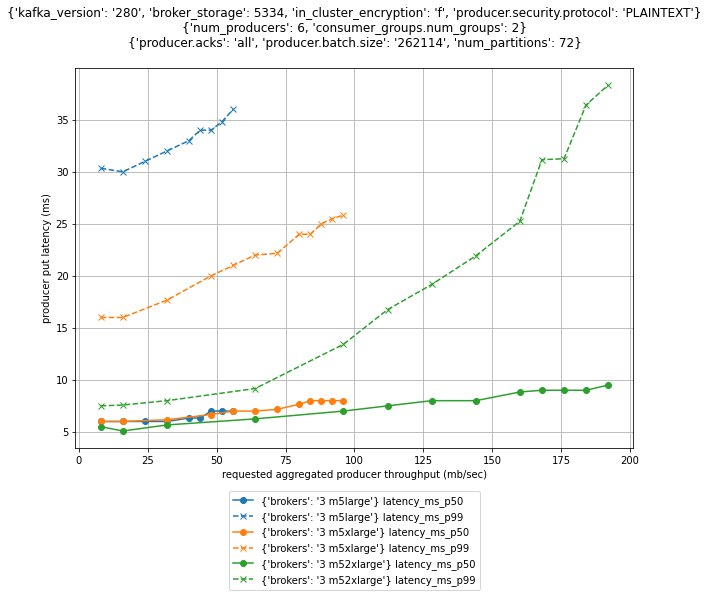
The following figure compares put latencies for three clusters with different broker sizes. For each cluster, the producers are running roughly a dozen individual performance tests with different throughput configurations. Initially, the producers produce a combined throughput of 16 MB/sec into the cluster and gradually increase the throughput with every individual test. Each individual test runs for 1 hour. For instances with burstable performance characteristics, credits are depleted before starting the actual performance measurement.

For brokers with more than 334 GB of storage, we can assume the EBS volume has a baseline throughput of 250 MB/sec. The Amazon EBS network baseline throughput is 81.25, 143.75, 287.5, and 593.75 MB/sec for the different broker sizes (for more information, see Supported instance types). The Amazon EC2 network baseline throughput is 96, 160, 320, and 640 MB/sec (for more information, see Network performance). Note that this only considers the sustained throughput; we discuss burst performance in a later section.
For a three-node cluster with replication 3 and two consumer groups, the recommended ingress throughput limits as per Equation 1 is as follows.
| Broker size |
Recommended sustained throughput limit |
| m5.large |
58 MB/sec |
| m5.xlarge |
96 MB/sec |
| m5.2xlarge |
192 MB/sec |
| m5.4xlarge |
200 MB/sec |
Even though the m5.4xlarge brokers have twice the number of vCPUs and memory compared to m5.2xlarge brokers, the cluster sustained throughput limit barely increases when scaling the brokers from m5.2xlarge to m5.4xlarge. That’s because with this configuration, the EBS volume used by brokers becomes a bottleneck. Remember that we’ve assumed a baseline throughput of 250 MB/sec for these volumes. For a three-node cluster and replication factor of 3, each broker needs to write the same traffic to the EBS volume as is sent to the cluster itself. And because the 80% of the baseline throughput of the EBS volume is 200 MB/sec, the recommended sustained throughput limit of the cluster with m5.4xlarge brokers is 200 MB/sec.
The next section describes how you can use provisioned throughput to increase the baseline throughput of EBS volumes and therefore increase the sustained throughput limit of the entire cluster.
Increase broker throughput with provisioned throughput
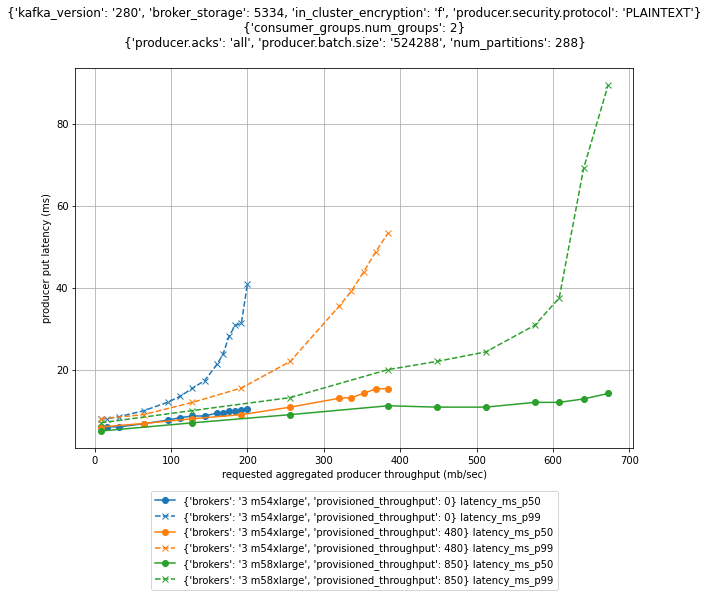
From the previous results, you can see that from a pure throughput perspective there is little benefit to increasing the broker size from m5.2xlarge to m5.4xlarge with the default cluster configuration. The baseline throughput of the EBS volume used by brokers limits their throughput. However, Amazon MSK recently launched the ability to provision storage throughput up to 1000 MB/sec. For self-managed clusters you can use gp3, io2, or st1 volume types to achieve a similar effect. Depending on the broker size, this can substantially increase the overall cluster throughput.
The following figure compares the cluster throughput and put latencies of different broker sizes and different provisioned throughput configurations.
For a three-node cluster with replication 3 and two consumer groups, the recommended ingress throughput limits as per Equation 1 are as follows.
| Broker size |
Provisioned throughput configuration |
Recommended sustained throughput limit |
| m5.4xlarge |
– |
200 MB/sec |
| m5.4xlarge |
480 MB/sec |
384 MB/sec |
| m5.8xlarge |
850 MB/sec |
680 MB/sec |
| m5.12xlarge |
1000 MB/sec |
800 MB/sec |
| m5.16xlarge |
1000 MB/sec |
800 MB/sec |
The provisioned throughput configuration was carefully chosen for the given workload. With two consumer groups consuming from the cluster, it doesn’t make sense to increase the provisioned throughput of m4.4xlarge brokers beyond the 480 MB/sec. The Amazon EC2 network, not the EBS volume throughput, restricts the recommended sustained throughput limit of the cluster to 384 MB/sec. But for workloads with a different number of consumers, it can make sense to further increase or decrease the provisioned throughput configuration to match the baseline throughput of the Amazon EC2 network.
Scale out to increase cluster write throughput
Scaling out the cluster naturally increases the cluster throughput. But how does this affect performance and cost? Let’s compare the throughput of two different clusters: a three-node m5.4xlarge and a six-node m5.2xlarge cluster, as shown in the following figure. The storage size for the m5.4xlarge cluster has been adapted so that both clusters have the same total storage capacity and therefore the cost for these clusters is identical.

The six-node cluster has almost double the throughput of the three-node cluster and substantially lower p99 put latencies. Just looking at ingress throughput of the cluster, it can make sense to scale out rather than to scale up, if you need more that 200 MB/sec of throughput. The following table summarizes these recommendations.
| Number of brokers |
Recommended sustained throughput limit |
| m5.large |
m5.2xlarge |
m5.4xlarge |
| 3 |
58 MB/sec |
192 MB/sec |
200 MB/sec |
| 6 |
115 MB/sec |
384 MB/sec |
400 MB/sec |
| 9 |
173 MB/sec |
576 MB/sec |
600 MB/sec |
In this case, we could have also used provisioned throughput to increase the throughput of the cluster. Compare, for instance, the sustained throughput limit of the six-node m5.2xlarge cluster in the preceding figure with that of the three-node m5.4xlarge cluster with provisioned throughput from the earlier example. The sustained throughput limit of both clusters is identical, which is caused by the same Amazon EC2 network bandwidth limit that usually grows proportional with the broker size.
Scale up to increase cluster read throughput
The more consumer groups are reading from the cluster, the more data egresses over the Amazon EC2 network of the brokers. Larger brokers have a higher network baseline throughput (up to 25 Gb/sec) and can therefore support more consumer groups reading from the cluster.
The following figure compares how latency and throughput changes for the different number of consumer groups for a three-node m5.2xlarge cluster.
As demonstrated in this figure, increasing the number of consumer groups reading from a cluster decreases its sustained throughput limit. The more consumers that consumer groups are reading from the cluster, the more data that needs to egress from the brokers over the Amazon EC2 network. The following table summarizes these recommendations.
| Consumer groups |
Recommended sustained throughput limit |
| m5.large |
m5.2xlarge |
m5.4xlarge |
| 0 |
65 MB/sec |
200 MB/sec |
200 MB/sec |
| 2 |
58 MB/sec |
192 MB/sec |
200 MB/sec |
| 4 |
38 MB/sec |
128 MB/sec |
200 MB/sec |
| 6 |
29 MB/sec |
96 MB/sec |
192 MB/sec |
The broker size determines the Amazon EC2 network throughput, and there is no way to increase it other than scaling up. Accordingly, to scale the read throughput of the cluster, you either need to scale up brokers or increase the number of brokers.
Balance broker size and number of brokers
When sizing a cluster, you often have the choice to either scale out or scale up to increase the throughput and performance of a cluster. Assuming storage size is adjusted accordingly, the cost of those two options is often identical. So when should you scale out or scale up?
Using smaller brokers allows you to scale the capacity in smaller increments. Amazon MSK enforces that brokers are evenly balanced across all configured Availability Zones. You can therefore only add a number of brokers that are a multiple of the number of Availability Zones. For instance, if you add three brokers to a three-node m5.4xlarge cluster with provisioned throughput, you increase the recommended sustained cluster throughput limit by 100%, from 384 MB/sec to 768 MB/sec. However, if you add three brokers to a six-node m5.2xlarge cluster, you increase the recommended cluster throughput limit by 50%, from 384 MB/sec to 576 MB/sec.
Having too few very large brokers also increases the blast radius in case a single broker is down for maintenance or because of failure of the underlying infrastructure. For instance, for a three-node cluster, a single broker corresponds to 33% of the cluster capacity, whereas it’s only 17% for a six-node cluster. When provisioning clusters to best practices, you have added enough spare capacity to not impact your workload during these operations. But for larger brokers, you may need to add more spare capacity than required because of the larger capacity increments.
However, the more brokers are part of the cluster, the longer it takes for maintenance and update operations to complete. The service applies these changes sequentially to one broker at a time to minimize impact to the availability of the cluster. When provisioning clusters to best practices, you have added enough spare capacity to not impact your workload during these operations. But the time it takes to complete the operation is still something to consider because you need to wait for one operation to complete before you can run another one.
You need to find a balance that works for your workload. Small brokers are more flexible because they give you smaller capacity increments. But having too many small brokers increases the time it takes for maintenance operations to complete and increase the likelihood for failure. Clusters with fewer larger brokers complete update operations faster. But they come with larger capacity increments and a higher blast radius in case of broker failure.
Scale up for CPU intensive workloads
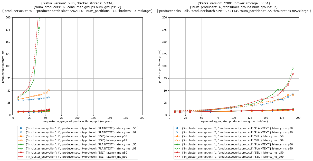
So far, we have we have focused on the network throughput of brokers. But there are other factors that determine the throughput and latency of the cluster. One of them is encryption. Apache Kafka has several layers where encryption can protect data in transit and at rest: encryption of the data stored on the storage volumes, encryption of traffic between brokers, and encryption of traffic between clients and brokers.
Amazon MSK always encrypts your data at rest. You can specify the AWS Key Management Service (AWS KMS) customer master key (CMK) that you want Amazon MSK to use to encrypt your data at rest. If you don’t specify a CMK, Amazon MSK creates an AWS managed CMK for you and uses it on your behalf. For data that is in-flight, you can choose to enable encryption of data between producers and brokers (in-transit encryption), between brokers (in-cluster encryption), or both.
Turning on in-cluster encryption forces the brokers to encrypt and decrypt individual messages. Therefore, sending messages over the network can no longer take advantage of the efficient zero copy operation. This results in additional CPU and memory bandwidth overhead.
The following figure shows the performance impact for these options for three-node clusters with m5.large and m5.2xlarge brokers.

For p99 put latencies, there is a substantial performance impact of enabling in-cluster encryption. As shown in the preceding graphs, scaling up brokers can mitigate the effect. The p99 put latency at 52 MB/sec throughput of an m5.large cluster with in-transit and in-cluster encryption is above 200 milliseconds (red and green dashed line in the left graph). Scaling the cluster to m5.2xlarge brokers brings down the p99 put latency at the same throughput to below 15 milliseconds (red and green dashed line in the right graph).
There are other factors that can increase CPU requirements. Compression as well as log compaction can also impact the load on clusters.
Scale up for a consumer not reading from the tip of the stream
We have designed the performance tests such that consumers are always reading from the tip of the topic. This effectively means that brokers can serve the reads from consumers directly from memory, not causing any read I/O to Amazon EBS. In contrast to all other sections of the post, we drop this assumption to understand how consumers that have fallen behind can impact cluster performance. The following diagram illustrates this design.

When a consumer falls behind or needs to recover from failure it reprocesses older messages. In that case, the pages holding the data may no longer reside in the page cache, and brokers need to fetch the data from the EBS volume. That causes additional network traffic to the volume and non-sequential I/O reads. This can substantially impact the throughput of the EBS volume.
In an extreme case, a backfill operation can reprocess the complete history of events. In that case, the operation not only causes additional I/O to the EBS volume, it also loads a lot of pages holding historic data into the page cache, effectively evicting pages that are holding more recent data. Consequently, consumers that are slightly behind the tip of the topic and would usually read directly from the page cache may now cause additional I/O to the EBS volume because the backfill operation has evicted the page they need to read from memory.
One option to mitigate these scenarios is to enable compression. By compressing the raw data, brokers can keep more data in the page cache before it’s evicted from memory. However, keep in mind that compression requires more CPU resources. If you can’t enable compression or if enabling compression can’t mitigate this scenario, you can also increase the size of the page cache by increasing the memory available to brokers by scaling up.
Use burst performance to accommodate traffic spikes
So far, we’ve been looking at the sustained throughput limit of clusters. That’s the throughput the cluster can sustain indefinitely. For streaming workloads, it’s important to understand baseline the throughput requirements and size accordingly. However, the Amazon EC2 network, Amazon EBS network, and Amazon EBS storage system are based on a credit system; they provide a certain baseline throughput and can burst to a higher throughput for a certain period based on the instance size. This directly translates to the throughput of MSK clusters. MSK clusters have a sustained throughput limit and can burst to a higher throughput for short periods.
The blue line in the following graph shows the aggregate throughput of a three-node m5.large cluster with two consumer groups. During the entire experiment, producers are trying to send data as quickly as possible into the cluster. So, although 80% of the sustained throughput limit of the cluster is around 58 MB/sec, the cluster can burst to a throughput well above 200 MB/sec for almost half an hour.

Think of it this way: When configuring the underlying infrastructure of a cluster, you’re basically provisioning a cluster with a certain sustained throughput limit. Given the burst capabilities, the cluster can then instantaneously absorb much higher throughput for some time. For instance, if the average throughput of your workload is usually around 50 MB/sec, the three-node m5.large cluster in the preceding graph can ingress more than four times its usual throughput for roughly half an hour. And that’s without any changes required. This burst to a higher throughput is completely transparent and doesn’t require any scaling operation.
This is a very powerful way to absorb sudden throughput spikes without scaling your cluster, which takes time to complete. Moreover, the additional capacity also helps in response to operational events. For instance, when brokers are undergoing maintenance or partitions need to be rebalanced within the cluster, they can use burst performance to get brokers online and back in sync more quickly. The burst capacity is also very valuable to quickly recover from operational events that affect an entire Availability Zone and cause a lot of replication traffic in response to the event.
Monitoring and continuous optimization
So far, we have focused on the initial sizing of your cluster. But after you determine the correct initial cluster size, the sizing efforts shouldn’t stop. It’s important to keep reviewing your workload after it’s running in production to know if the broker size is still appropriate. Your initial assumptions may no longer hold in practice, or your design goals might have changed. After all, one of the great benefits of cloud computing is that you can adapt the underlying infrastructure through an API call.
As we have mentioned before, the throughput of your production clusters should target 80% of their sustained throughput limit. When the underlying infrastructure is starting to experience throttling because it has exceeded the throughput limit for too long, you need to scale up the cluster. Ideally, you would even scale the cluster before it reaches this point. By default, Amazon MSK exposes three metrics that indicate when this throttling is applied to the underlying infrastructure:
- BurstBalance – Indicates the remaining balance of I/O burst credits for EBS volumes. If this metric starts to drop, consider increasing the size of the EBS volume to increase the volume baseline performance. If Amazon CloudWatch isn’t reporting this metric for your cluster, your volumes are larger than 5.3 TB and no longer subject to burst credits.
- CPUCreditBalance – Only relevant for brokers of the T3 family and indicates the amount of available CPU credits. When this metric starts to drop, brokers are consuming CPU credits to burst beyond their CPU baseline performance. Consider changing the broker type to the M5 family.
- TrafficShaping – A high-level metric indicating the number of packets dropped due to exceeding network allocations. Finer detail is available when the
PER_BROKER monitoring level is configured for the cluster. Scale up brokers if this metric is elevated during your typical workloads.
In the previous example, we saw the cluster throughput drop substantially after network credits were depleted and traffic shaping was applied. Even if we didn’t know the maximum sustained throughput limit of the cluster, the TrafficShaping metric in the following graph clearly indicates that we need to scale up the brokers to avoid further throttling on the Amazon EC2 network layer.

Amazon MSK exposes additional metrics that help you understand whether your cluster is over- or under-provisioned. As part of the sizing exercise, you have determined the sustained throughput limit of your cluster. You can monitor or even create alarms on the BytesInPerSec, ReplicationBytesInPerSec, BytesOutPerSec, and ReplicationBytesInPerSec metrics of the cluster to receive notification when the current cluster size is no longer optimal for the current workload characteristics. Likewise, you can monitor the CPUIdle metric and alarm when your cluster is under- or over-provisioned in terms of CPU utilization.
Those are only the most relevant metrics to monitor the size of your cluster from an infrastructure perspective. You should also monitor the health of the cluster and the entire workload. For further guidance on monitoring clusters, refer to Best Practices.
A framework for testing Apache Kafka performance
As mentioned before, you must run your own tests to verify if the performance of a cluster matches your specific workload characteristics. We have published a performance testing framework on GitHub that helps automate the scheduling and visualization of many tests. We have been using the same framework to generate the graphs that we have been discussing in this post.
The framework is based on the kafka-producer-perf-test.sh and kafka-consumer-perf-test.sh tools that are part of the Apache Kafka distribution. It builds automation and visualization around these tools.
For smaller brokers that are subject to bust capabilities, you can also configure the framework to first generate excess load over an extended period to deplete networking, storage, or storage network credits. After the credit depletion completes, the framework runs the actual performance test. This is important to measure the performance of clusters that can be sustained indefinitely rather than measuring peak performance, which can only be sustained for some time.
To run your own test, refer to the GitHub repository, where you can find the AWS Cloud Development Kit (AWS CDK) template and additional documentation on how to configure, run, and visualize the results of performance test.
Conclusion
We’ve discussed various factors that contribute to the performance of Apache Kafka from an infrastructure perspective. Although we’ve focused on Apache Kafka, we also learned about Amazon EC2 networking and Amazon EBS performance characteristics.
To find the right size for your clusters, work backward from your use case to determine the throughput, availability, durability, and latency requirements.
Start with an initial sizing of your cluster based on your throughput, storage, and durability requirements. Scale out or use provisioned throughput to increase the write throughput of the cluster. Scale up to increase the number of consumers that can consume from the cluster. Scale up to facilitate in-transit or in-cluster encryption and consumers that aren’t reading form the tip of the stream.
Verify this initial cluster sizing by running performance tests and then fine-tune the cluster size and configuration to match other requirements, such as latency. Add additional capacity for production clusters so that they can withstand the maintenance or loss of a broker. Depending on your workload, you may even consider withstanding an event affecting an entire Availability Zone. Finally, keep monitoring your cluster metrics and resize the cluster in case your initial assumptions no longer hold.
About the Author
 Steffen Hausmann is a Principal Streaming Architect at AWS. He works with customers around the globe to design and build streaming architectures so that they can get value from analyzing their streaming data. He holds a doctorate degree in computer science from the University of Munich and in his free time, he tries to lure his daughters into tech with cute stickers he collects at conferences.


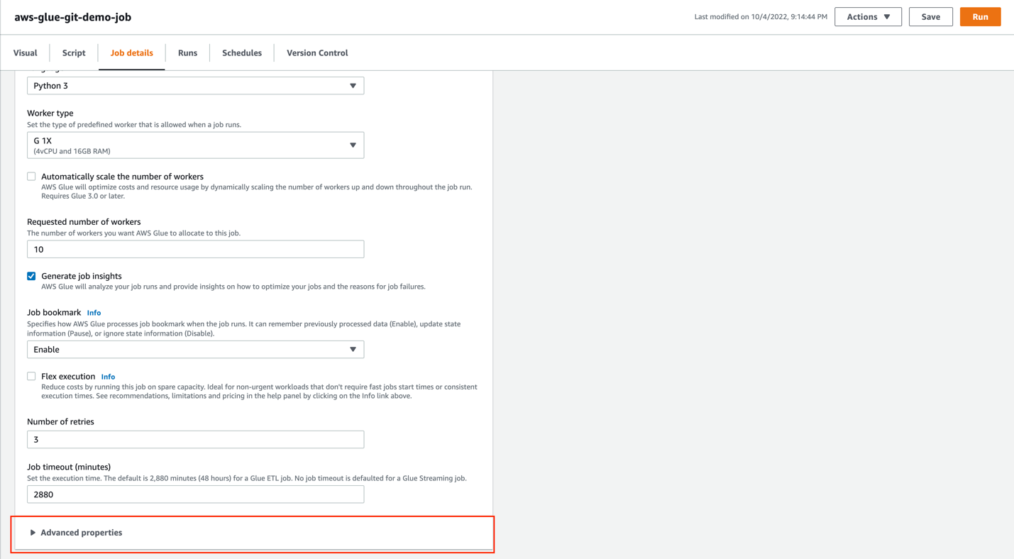
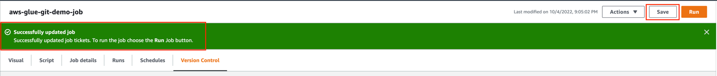
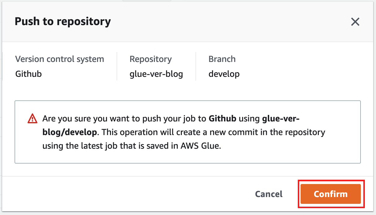
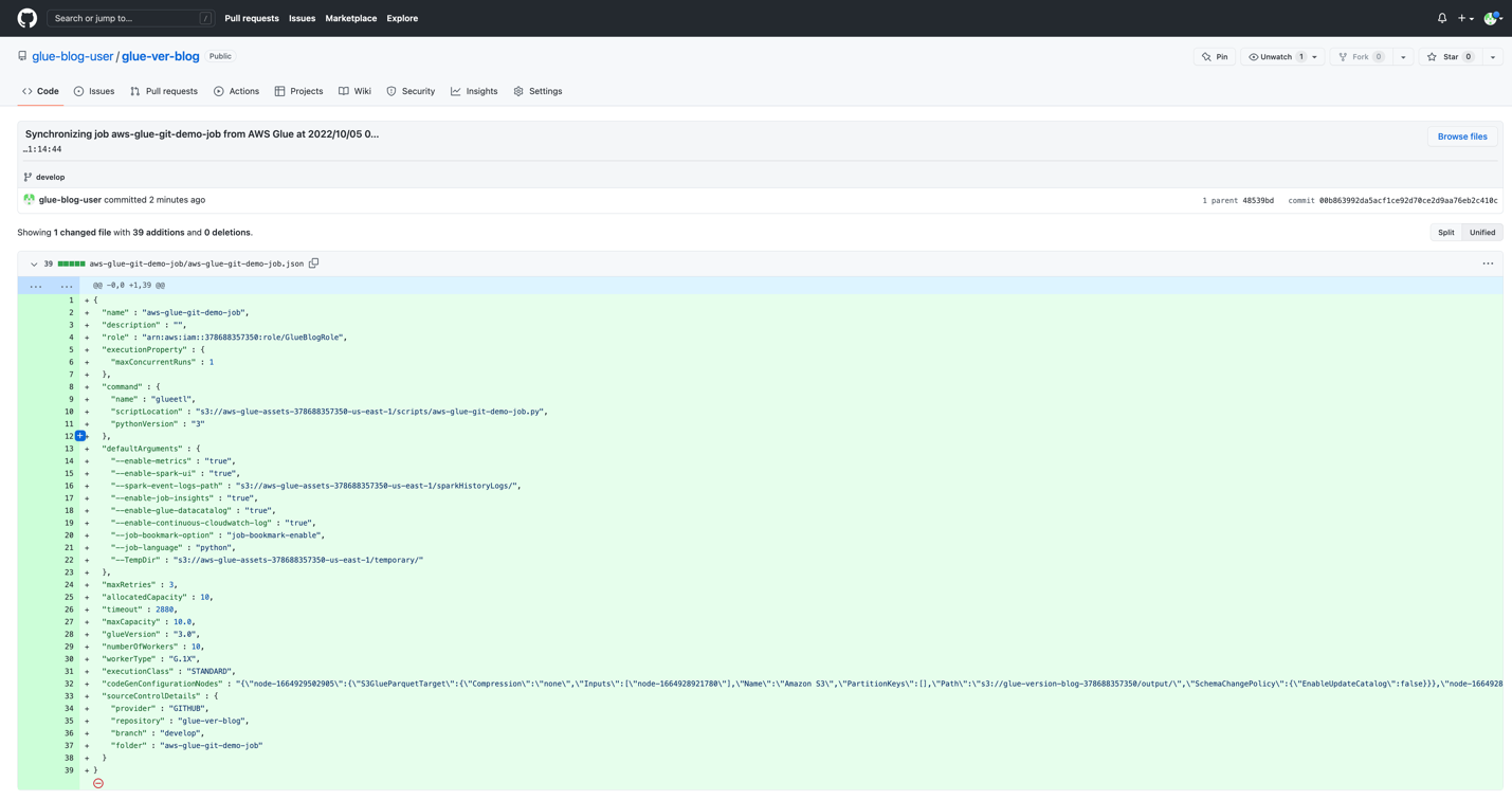
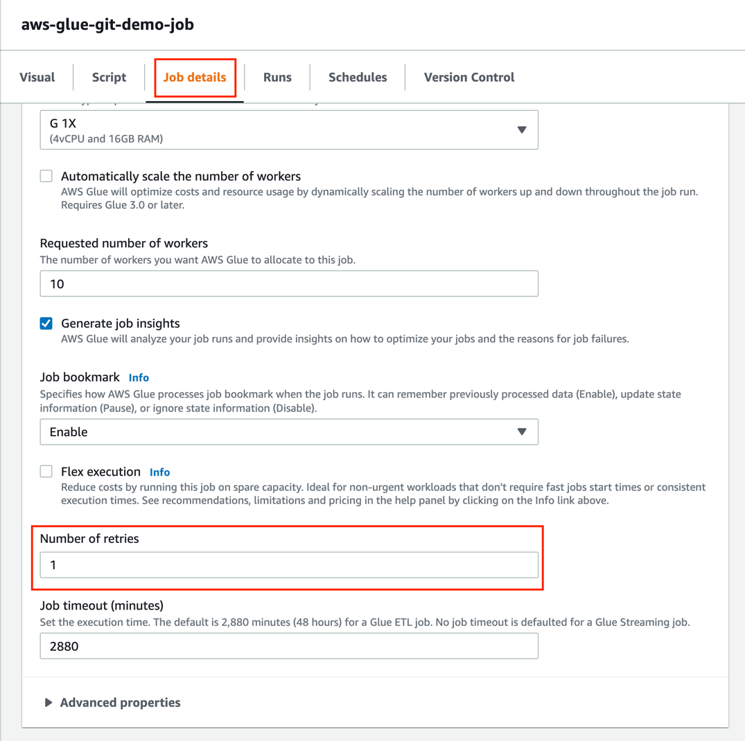
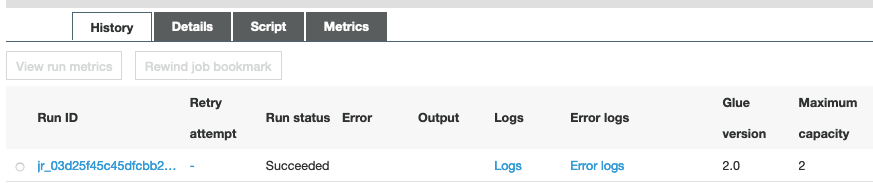
 Now the job is ready to be pushed into the develop branch of our version control system.


 Leonardo Gómez is a Senior Analytics Specialist Solutions Architect at AWS. Based in Toronto, Canada, he has over a decade of experience in data management, helping customers around the globe address their business and technical needs.
 Daiyan Alamgir is a Principal Frontend Engineer on AWS Glue based in New York. He leads the AWS Glue UI team and is focused on building interactive web-based applications for data analysts and engineers to address their data integration use cases.


 Rahul Chaturvedi is an Analytics Specialist Solutions Architect at AWS. Prior to this role, he was a Data Engineer at Amazon Advertising and Prime Video, where he helped build petabyte-scale data lakes for self-serve analytics.


 Hari Ohm Prasath is a Senior Modernization Architect at AWS, helping customers with their modernization journey to become cloud native. Hari loves to code and actively contributes to the open source initiatives. You can find him in Medium, Github & Twitter @hariohmprasath.
 Ballu Singh is a Principal Solutions Architect at AWS. He lives in the San Francisco Bay area and helps customers architect and optimize applications on AWS. In his spare time, he enjoys reading and spending time with his family.


 Noritaka Sekiyama is a Senior Big Data Architect at AWS Glue & Lake Formation. His passion is for implementing software artifacts for building data lakes more effectively and easily. During his spare time, he loves to spend time with his family, especially hunting bugs—not software bugs, but bugs like butterflies, pill bugs, snails, and grasshoppers.
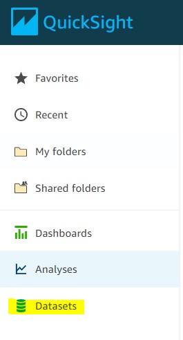
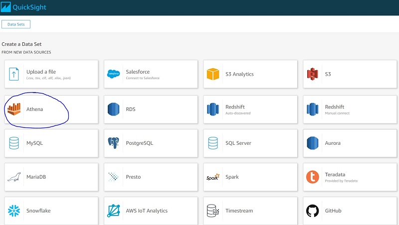
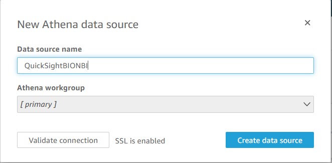
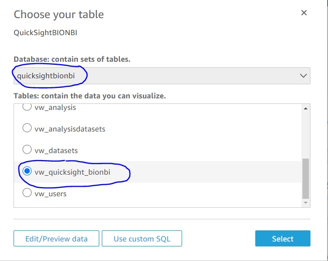
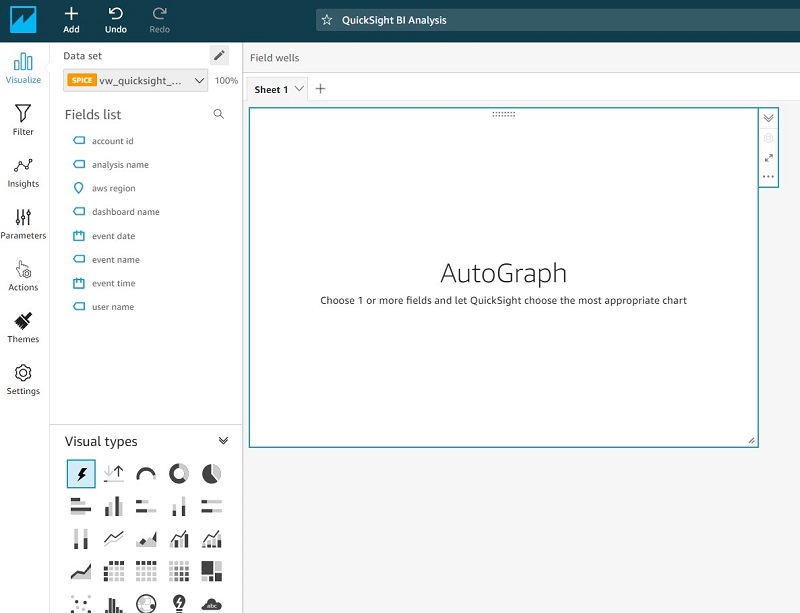
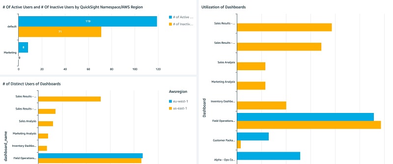
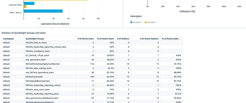
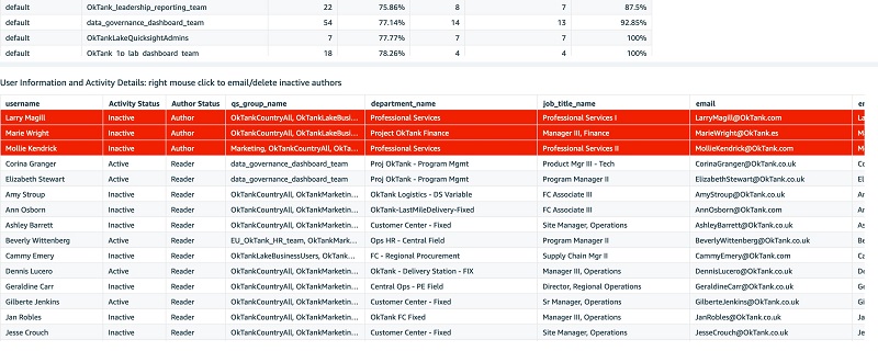
 QuickSight visualization


 Sunil Salunkhe is a Senior Solution Architect working with Strategic Accounts on their vision to leverage the cloud to drive aggressive growth strategies. He practices customer obsession by solving their complex challenges in all the aspects of the cloud journey including scale, security and reliability. While not working, he enjoys playing cricket and go cycling with his wife and a son.
 Nihar Sheth is a Senior Product Manager on the Amazon Kinesis Data Streams team at Amazon Web Services. He is passionate about developing intuitive product experiences that solve complex customer problems and enables customers to achieve their business goals. Outside of work, he is focusing on hiking 200 miles of beautiful PNW trails with his son in 2021.
 Karthi Thyagarajan is a Solutions Architect on the Amazon Kinesis Team focusing on all things streaming and he enjoys helping customers tackle distributed systems challenges.
 Sai Maddali is a Sr. Product Manager – Tech at Amazon Web Services where he works on Amazon Kinesis Data Streams . He is passionate about understanding customer needs, and using technology to deliver services that empowers customers to build innovative applications. Besides work, he enjoys traveling, cooking, and running.
 Larry Heathcote is a Senior Product Marketing Manager at Amazon Web Services for data streaming and analytics. Larry is passionate about seeing the results of data-driven insights on business outcomes. He enjoys walking his Samoyed Sasha in the mornings so she can look for squirrels to bark at.


 Gopalakrishnan Ramaswamy is a Solutions Architect at AWS based out of India with extensive background in database, analytics, and machine learning. He helps customers of all sizes solve complex challenges by providing solutions using AWS products and services. Outside of work, he likes the outdoors, physical activities and spending time with friends and family.


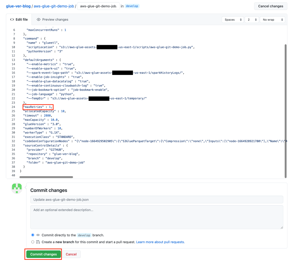
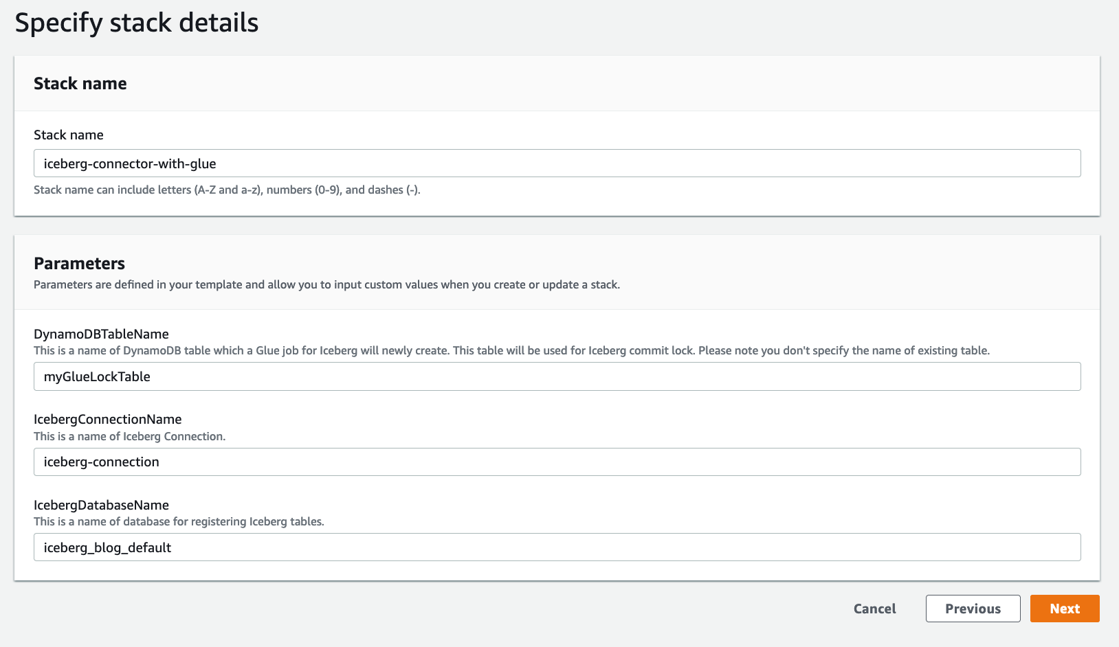
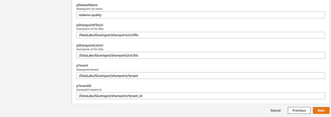
 Similarly, we can create other parameters such as


 The following screenshots show the Dashboards Analysis tab.
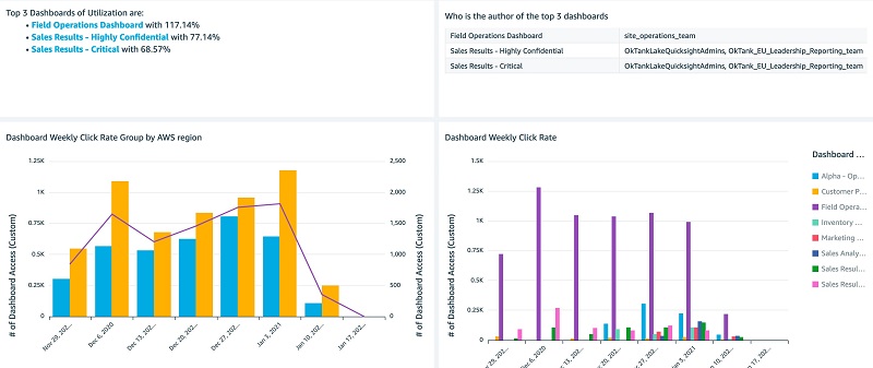
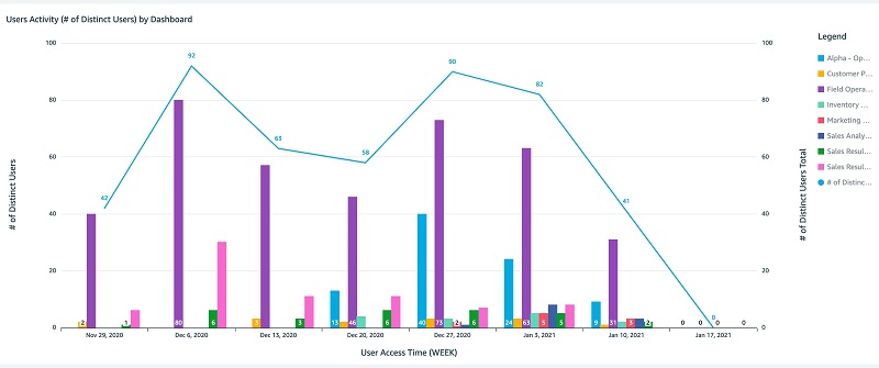
 You can interactively play with the sample dashboard in the following
  Ying Wang is a Data Visualization Engineer with the Data & Analytics Global Specialty Practice in AWS Professional Services.
 Jill Florant manages Customer Success for the Amazon QuickSight Service team


 Pablo Redondo Sanchez is a Senior Solutions Architect at Amazon Web Services. He is a data enthusiast and works with customers to help them achieve better insights and faster outcomes from their data analytics workflows. In his spare time, Pablo enjoys woodworking and spending time outdoor with his family in Northern California.


 Conclusion
 Jeff Wright is a Software Development Engineer at Amazon Web Services where he works on the Search Services team. His interests are designing and building robust, scalable distributed applications. Jeff is a contributor to Open Distro for Elasticsearch.
 Kowshik Nagarajaan is a Software Development Engineer at Amazon Web Services where he works on the Search Services team. His interests are building and automating distributed analytics applications. Kowshik is a contributor to Open Distro for Elasticsearch.
 Anush Krishnamurthy is an Engineering Manager working on the Search Services team at Amazon Web Services.