Post Syndicated from Francisco Oliveira original https://aws.amazon.com/blogs/big-data/multi-tenant-processing-pipelines-with-aws-dms-aws-step-functions-and-apache-hudi-on-amazon-emr/
Large enterprises often provide software offerings to multiple customers by providing each customer a dedicated and isolated environment (a software offering composed of multiple single-tenant environments). Because the data is in various independent systems, large enterprises are looking for ways to simplify data processing pipelines. To address this, you can create data lakes to bring your data to a single place.
Typically, a replication tool such as AWS Database Migration Service (AWS DMS) can replicate the data from your source systems to Amazon Simple Storage Service (Amazon S3). When the data is in Amazon S3, you process it based on your requirements. A typical requirement is to sync the data in Amazon S3 with the updates on the source systems. Although it’s easy to apply updates on a relational database management system (RDBMS) that backs an online source application, it’s tough to apply this change data capture (CDC) process on your data lakes. Apache Hudi is a good way to solve this problem. You can use Hudi on Amazon EMR to create Hudi tables (for more information, see Hudi in the Amazon EMR Release Guide).
This post introduces a pipeline that loads data and its ongoing changes (change data capture) from multiple single-tenant tables from different databases to a single multi-tenant table in an Amazon S3-backed data lake, simplifying data processing activities by creating multi-tenant datasets.
Architecture overview
At a high level, this architecture consolidates multiple single-tenant environments into a single multi-tenant dataset so data processing pipelines can be centralized. For example, suppose that your software offering has two tenants, each with their dedicated and isolated environment, and you want to maintain a single multi-tenant table that includes data of both tenants. Moreover, you want any ongoing replication (CDC) in the sources for tenant 1 and tenant 2 to be synchronized (compacted or reconciled) when an insert, delete, or update occurs in the source systems of the respective tenant.
In the past, to support record-level updates or inserts (called upserts) and deletes on an Amazon S3-backed data lake, you relied on either having an Amazon Redshift cluster or an Apache Spark job that reconciled the update, deletes, and inserts with existing historical data.
The architecture for our solution uses Hudi to simplify incremental data processing and data pipeline development by providing record-level insert, update, upsert, and delete capabilities. For more information, see Apache Hudi on Amazon EMR.
Moreover, the architecture for our solution uses the following AWS services:
- AWS DMS – AWS DMS is a cloud service that makes it easy to migrate relational databases, data warehouses, NoSQL databases, and other types of data stores. For more information, see What is AWS Database Migration Service?
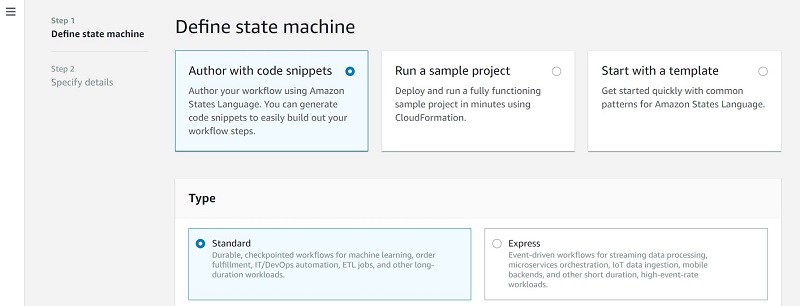
- AWS Step Functions – AWS Step Functions is a web service that enables you to coordinate the components of distributed applications and microservices using visual workflows. For more information, see What Is AWS Step Functions?
- Amazon EMR – Amazon EMR is a managed cluster platform that simplifies running big data frameworks, such as Apache Hadoop and Apache Spark, on AWS to process and analyze vast amounts of data. For more information, see Overview of Amazon EMR Architecture and Overview of Amazon EMR.
- Amazon S3 – Data is stored in Amazon S3, an object storage service with scalable performance, ease-of-use features, and native encryption and access control capabilities. For more details on Amazon S3, see Amazon S3 as the Data Lake Storage Platform.
Architecture deep dive
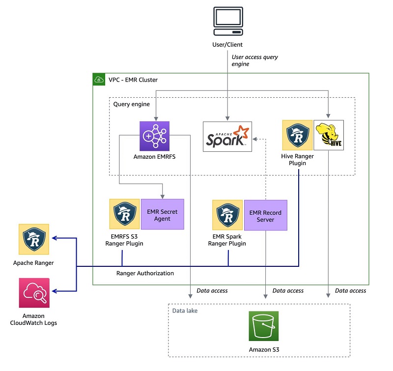
The following diagram illustrates our architecture.

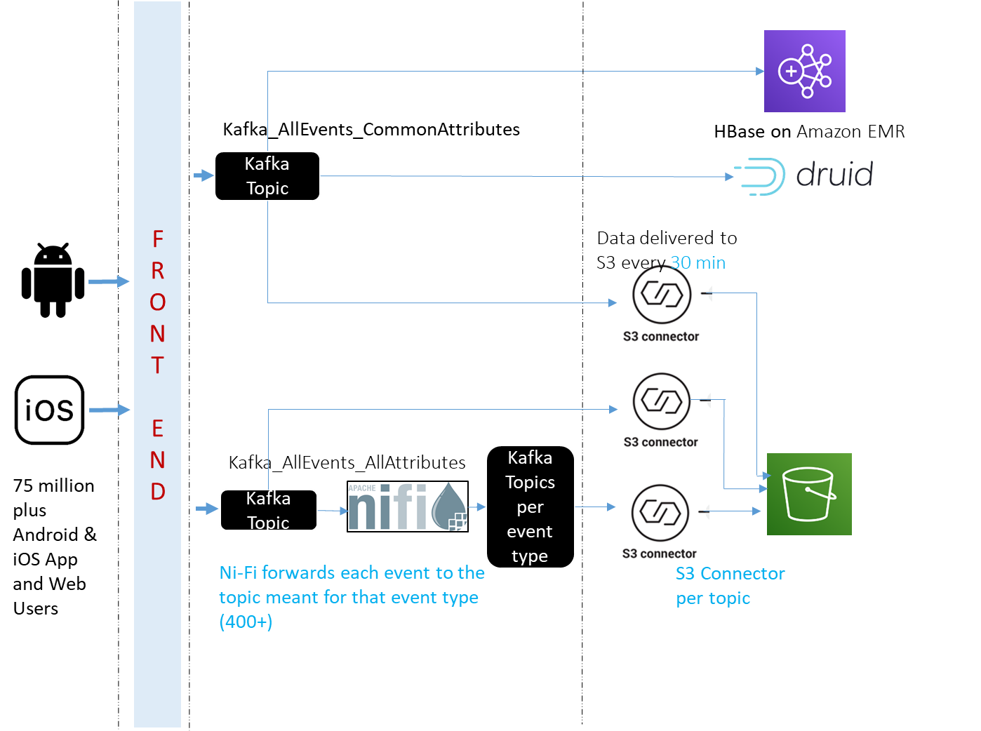
This architecture relies on AWS Database Migration Service (AWS DMS) to transfer data from specific tables into an Amazon S3 location organized by tenant-id.
Although AWS DMS performs the migration and the ongoing replication—also known as change data capture (CDC)—it applies a data transformation that adds a custom column named tenant-id and populates it with the tenant-id value defined in the AWS DMS migration task configuration. The AWS DMS data transformations allow you to modify a schema, table, or column or, in this case, add a column with the tenant-id so data transferred to Amazon S3 is grouped by tenant-id.
AWS DMS is also configured to add an additional column with timestamp information. For a full load, each row of this timestamp column contains a timestamp for when the data was transferred from the source to the target by AWS DMS. For ongoing replication, each row of the timestamp column contains the timestamp for the commit of that row in the source database.
We use an AWS Step Functions workflow to move the files AWS DMS wrote to Amazon S3 into an Amazon S3 location that is organized by table name and holds all the tenant’s data. Files in this location all have the new column tenant-id, and the respective tenant-id value is configured in the AWS DMS task configuration.
Next, the Hudi DeltaStreamer utility runs on Amazon EMR to process the multi-tenant source data and create or update the Hudi dataset on Amazon S3.
You can pass to the Hudi DeltaStreamer utility a field in the data that has each record’s timestamp. The Hudi DeltaStreamer utility uses this to ensure records are processed in the proper chronological order. You can also provide the Hudi DeltaStreamer utility one or more SQL transforms, which the utility applies in a sequence as records are read and before the datasets are persisted on Amazon S3 as an Hudi Parquet dataset. We highlight the SQL transform later in this post.
Depending on your downstream consumption patterns, you might require a partitioned dataset. We discuss the process to choose a partition within Hudi DeltaStreamer later in this post.
For this post, we use the Hudi DeltaStreamer utility instead of the Hudi DataSource due to its operational simplicity. However, you can also use Hudi DataSource with this pattern.
When to use and not use this architecture
This architecture is ideal for the workloads that are processed in batches and can tolerate the latency associated with the time required to capture the changes in the sources, write those changes into objects in Amazon S3, and run the Step Functions workflow that aggregates the objects per tenant and creates the multi-tenant Hudi dataset.
This architecture uses and applies to Hudi COPY_ON_WRITE tables. This architecture is not recommended for latency-sensitive applications and does not support MERGE_ON_READ tables. For more information, see the section Analyzing the properties provided to the command to run the Hudi DeltaStreamer utility.
This architecture pattern is also recommended for workloads that have update rates to the same record (identified by a primary key) that are separated by, at most, microseconds or microsecond precision. The reason behind this is that Hudi uses a field, usually a timestamp, to break ties between records with the same key. If the field used to break ties can capture each individual update, data stored in the Hudi dataset on Amazon S3 is exactly the same as in the source system.
The precision of timestamp fields in your table depends on the database engine at the source. We strongly recommended that as you evaluate adopting this pattern, you also evaluate the support that AWS DMS provides to your current source engines, and understand the rate of updates in your source and the respective timestamp precision requirements that the source needs to support or currently supports. For example: AWS DMS writes any timestamp column values that are written to Amazon S3 as part of an ongoing replication with second precision if the data source is MySQL, and with microsecond precision if the data source is PostgreSQL. See the section Timestamp precision considerations for additional details.
This architecture assumes that all tables in every source database have the same schema and that any changes to a table’s schema is performed to each data source at the same time. Moreover, this architecture pattern assumes that any schema changes are backward compatible—you only append new fields and don’t delete any existing fields. Hudi supports schema evolutions that are backward compatible.
If you’re expecting constant schema changes to the sources, it might be beneficial to consider performing full snapshots instead of ingesting and processing the CDC. If performing full snapshots isn’t practical and you are expecting constant schema changes that are not compatible with Hudi’s schema evolution support, you can use the Hudi DataWriter API with your Spark jobs and address schema changes within the code by casting and adding columns as required to keep backward compatibility.
See the Schema evolution section for more details on the process for schema evolution with AWS DMS and Hudi.
Although it’s out of scope to evaluate the consumption tools available downstream to the Hudi dataset, you can consume Hudi datasets stored on Amazon S3 from Apache Hive, Spark, and Presto on Amazon EMR. Moreover, you can consume Hudi datasets stored on Amazon S3 from Amazon Redshift Spectrum and Amazon Athena.
Solution overview
This solution uses an AWS CloudFormation template to create the necessary resources.
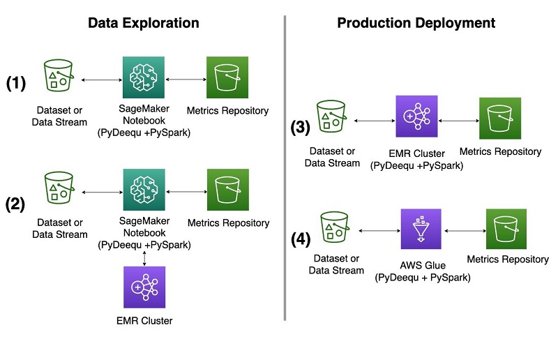
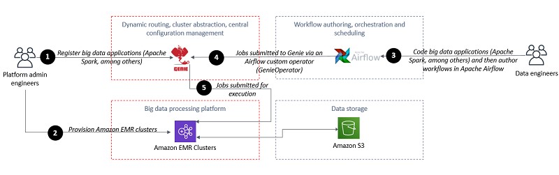
You trigger the Step Functions workflow via the AWS Management Console. The workflow uses AWS Lambda for processing tasks that are part of the logic. Moreover, the workflow submits jobs to an EMR cluster configured with Hudi.
To perform the database migration, the CloudFormation template deploys one AWS DMS replication instance and configures two AWS DMS replications tasks, one per tenant. The AWS DMS replication tasks connect to the source data stores, read the source data, apply any transformations, and load the data into the target data store.
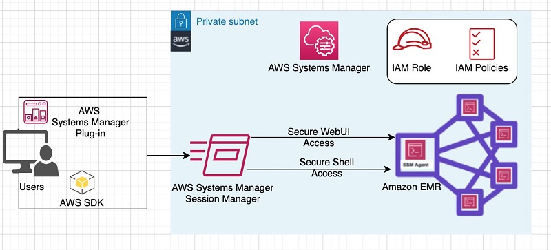
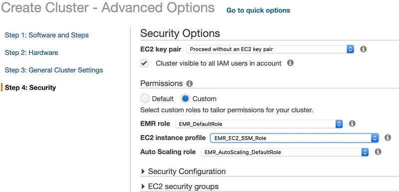
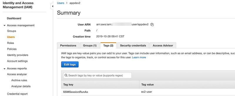
You access an Amazon SageMaker notebook to generate changes (updates) to the sources. Moreover, you connect into the Amazon EMR master node via AWS Systems Manager Session Manager to run Hive or Spark queries in the Hudi dataset backed by Amazon S3. Session Manager provides secure and auditable instance management without the need to open inbound ports, maintain bastion hosts, or manage SSH keys.
The following diagram illustrates the solution architecture.

The orchestration in this demo code currently supports processing at most 25 sources (tables within a database or distributed across multiple databases) per run and is not preventing concurrent runs of the same tenant-id, database-name, or table-name triplet by keeping track of the tenant-id, database-name, or table-name triplet being processed or already processed. Preventing concurrent runs avoids duplication of work. Moreover, the orchestration in this demo code doesn’t prevent the Hudi DeltaStreamer job to run with the output of both an AWS DMS full load task and an AWS DMS CDC load task. For production environments, we recommend that you keep track of the existing tenant_id in the multi-tenant Hudi dataset. This way, if an existing AWS DMS replication task is mistakenly restarted to perform a full load instead of continuing the ongoing replication, your solution can adequately prevent any downstream impact to the datasets. Moreover, we recommend that you keep track of the schema changes in the source and guarantee that the Hudi DeltaStreamer utility only processes files with the same schema.
For details on considerations related to the Step Functions workflows, see Best Practices for Step Functions. For more information about considerations when running AWS DMS at scale, see Best practices for AWS Database Migration Service. Finally, for details on how to tune Hudi, see Performance and Tuning Guide.
Next, we walk you through several key areas of the solution.
Prerequisites
Before getting started, you must create a S3 bucket, unzip and upload the blog artifacts to the S3 bucket and store the database passwords in AWS Systems Manager Parameter Store.
Creating and storing admin passwords in AWS Systems Manager Parameter Store
This solution uses AWS Systems Manager Parameter Store to store the passwords used in the configuration scripts. With Parameter Store, you can create secure string parameters, which are parameters that have a plaintext parameter name and an encrypted parameter value. Parameter Store uses AWS Key Management Service (AWS KMS) to encrypt and decrypt the parameter values of secure string parameters. With Parameter Store, you improve your security posture by separating your data from your code and by controlling and auditing access at granular levels. There is no charge from Parameter Store to create a secure string parameter, but charges for using AWS KMS do apply. For information, see AWS Key Management Service pricing.
Before deploying the CloudFormation templates, run the following AWS Command Line Interface (AWS CLI) commands. These commands create Parameter Store parameters to store the passwords for the RDS master user for each tenant.
aws ssm put-parameter --name "/HudiStack/RDS/Tenant1Settings" --type SecureString --value "ch4ng1ng-s3cr3t" --region Your-AWS-Region

aws ssm put-parameter --name "/HudiStack/RDS/Tenant2Settings" --type SecureString --value "ch4ng1ng-s3cr3t" --region Your-AWS-Region
AWS DMS isn’t integrated with Parameter Store, so you still need to set the same password as in the CloudFormation template parameter DatabasePassword (see the following section).
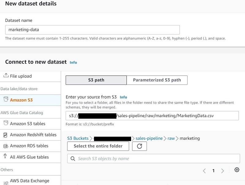
Creating an S3 bucket for the solution and uploading the solution artifacts to Amazon S3
This solution uses Amazon S3 to store all artifacts used in the solution. Before deploying the CloudFormation templates, create an Amazon S3 bucket and download the artifacts required by the solution.
Unzip the artifacts and upload all folders and files in the .zip file to the S3 bucket you just created.
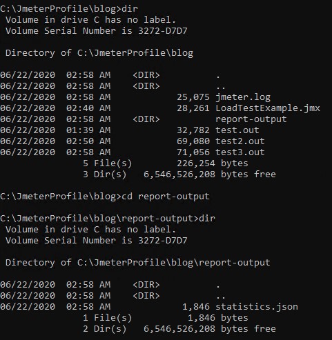
The following screenshot uses the root location hudistackbucket.

Keep a record of the Amazon S3 root path because you add it as a parameter to the CloudFormation template later.
Creating the CloudFormation stack
To launch the entire solution, choose Launch Stack:

The template requires the following parameters. You can accept the default values for any parameters not in the table. For the full list of parameters, see the CloudFormation template.
- S3HudiArtifacts – The bucket name that holds the solution artifacts (Lambda function Code, Amazon EMR step artifacts, Amazon SageMaker notebook, Hudi job configuration file template). You created this bucket in the previous step. For this post, we use
hudistackbucket.
- DatabasePassword – The database password. This value needs to be the same as the one configured via Parameter Store. The CloudFormation template uses this value to configure the AWS DMS endpoints.
- emrLogUri – The Amazon S3 location to store Amazon EMR cluster logs. For example,
s3://replace-with-your-bucket-name/emrlogs/.
Testing database connectivity
To test connectivity, complete the following steps:
- On the Amazon SageMaker Console, choose Notebook instances.
- Locate the notebook instance you created and choose Open Jupyter.
- In the new window, choose Runmev5.ipynb.
This opens the notebook for this post. We use the notebook to generate changes and updates to the databases used in the post.
- Run all cells of the notebook until the section Triggering the AWS DMS full load tasks for tenant 1 and tenant 2.
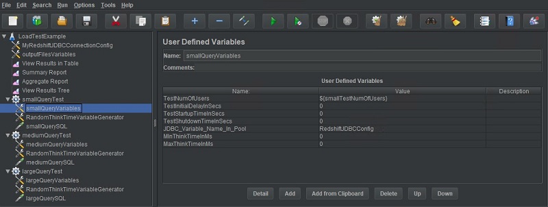
Analyzing the AWS DMS configuration
In this section, we examine the data transformation configuration and other AWS DMS configurations.
Data transformation configuration
To support the conversion from single-tenant to multi-tenant pipelines, the CloudFormation template applied a data transformation to the AWS DMS replication task. Specifically, the data transformation adds a new column named tenant_id to the Amazon S3 AWS DMS target. Adding the tenant_id column helps with downstream activities organize the datasets per tenant_id. For additional details on how to set up AWS DMS data transformation, see Transformation Rules and Actions. For reference, the following code is the data transformation we use for this post:
{
    "rules": [
        {
            "rule-type": "selection",
            "rule-id": "1",
            "rule-name": "1",
            "object-locator": {
                "schema-name": "salesdb",
                "table-name": "sales_order_detail"
            },
            "rule-action": "include",
            "filters": []
        },
        {
            "rule-type": "transformation",
            "rule-id": "2",
            "rule-name": "2",
            "rule-action": "add-column",
            "rule-target": "column",
            "object-locator": {
                "schema-name": "salesdb",
                "table-name": "sales_order_detail"
            },
            "value": "tenant_id",
            "expression": "1502",
            "data-type": {
                "type": "string",
                "length": 50
            }
        }
    ]
}
Other AWS DMS configurations
When using Amazon S3 as a target, AWS DMS accepts several configuration settings that provide control on how the files are written to Amazon S3. Specifically, for this use case, AWS DMS uses Parquet as the value for the configuration property DataFormat. For additional details on the S3 settings used by AWS DMS, see S3Settings. For reference, we use the following code:
DataFormat=parquet;TimestampColumnName=timestamp;
Timestamp precision considerations
By default, AWS DMS writes timestamp columns in a Parquet format with a microsecond precision, should the source engine support that precision. If the rate of updates you’re expecting is high, it’s recommended that you use a source that has support for microsecond precision, such as PostgreSQL.
Moreover, if the rate of updates is high, you might want to use a data source with microsecond precision and the AR_H_TIMESTAMP internal header column, which captures the timestamp of when the changes were made instead of the timestamp indicating the time of the commit. See Replicating source table headers using expressions for more details, specifically the details on the AR_H_TIMESTAMP internal header column. When you set TimestampColumnName=timestamp as we mention earlier, the new timestamp column captures the time of the commit.
If you need to use the AR_H_TIMESTAMP internal header column with a data source that supports microsecond precision such as PostgreSQL, we recommend using the Hudi DataSource writer job instead of the Hudi DeltaStreamer utility. The reason for this is that although the AR_H_TIMESTAMP internal header column (in a source that supports microsecond precision) has microsecond precision, the actual value written by AWS DMS on Amazon S3 has a nanosecond format (microsecond precision with the nanosecond dimension set to 0). By using the Hudi DataSource writer job, you can convert the AR_H_TIMESTAMP internal header column to a timestamp datatype in Spark with microsecond precision and use that new value as the PARTITIONPATH_FIELD_OPT_KEY. See Datasource Writer for more details.
Triggering the AWS DMS full load tasks for Tenant 1 and Tenant 2
In this step, we run a full load of data from both databases to Amazon S3 using AWS DMS. To accomplish this, perform the following steps:
- On the AWS DMS console, under Migration, choose Database migration tasks.
- Select the replication task for Tenant 1 (
dmsreplicationtasksourcetenant1-xxxxxxxxxxxxxxx).
- From the Actions menu, choose Restart/Resume.
- Repeat these steps for the Tenant 2 replication task.
You can monitor the progress of this task by choosing the task link.
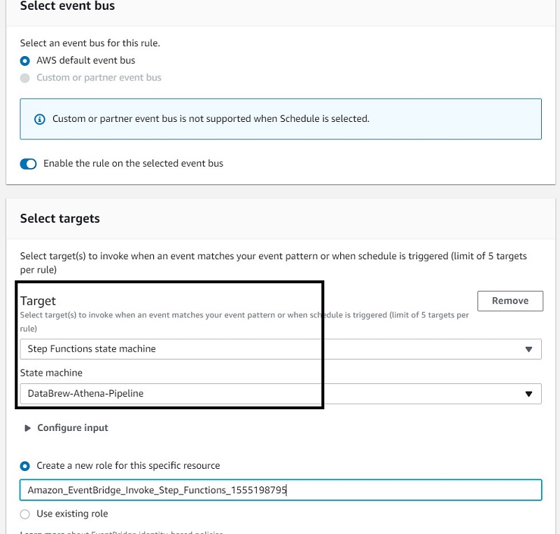
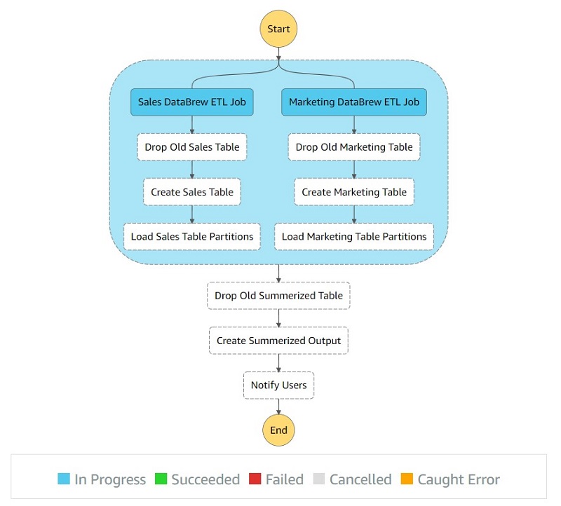
Triggering the Step Functions workflow
Next, we start a Step Functions workflow that automates the end-to-end process of processing the files loaded by AWS DMS to Amazon S3 and creating a multi-tenant Amazon S3-backed table using Hudi.
To trigger the Step Functions workflow, perform the following steps:
- On the Step Functions console, choose State machines.
- Choose the
MultiTenantProcessing workflow.
- In the new window, choose Start execution.
- Edit the following JSON code and replace the values as needed. You can find the
emrClusterId on the Outputs tab of the Cloudformation template.
{
  "hudiConfig": {
    "emrClusterId": "[REPLACE]",
    "targetBasePath": "s3://hudiblog-[REPLACE-WITH-YOUR-ACCOUNT-ID]/transformed/multitenant/huditables/sales_order_detail_mt",
"targetTable": "sales_order_detail_mt",
"sourceOrderingField": "timestamp",
"blogArtifactBucket": "[REPLACE-WITH-BUCKETNAME-WITH-BLOG-ARTIFACTS]",
"configScriptPath": "s3://[REPLACE-WITH-BUCKETNAME-WITH-BLOG-ARTIFACTS]/emr/copy_apache_hudi_deltastreamer_command_properties.sh",
"propertiesFilename": "dfs-source.properties"
},
  "copyConfig":{
            "srcBucketName": "hudiblog-[REPLACE-WITH-YOUR-ACCOUNT-ID]",
            "srcPrefix": "raw/singletenant/",
            "destBucketName": "hudiblog-[REPLACE-WITH-YOUR-ACCOUNT-ID]",
            "destPrefix": "raw/multitenant/salesdb/sales_order_detail_mt/"},
      "sourceConfig":{
            "databaseName": "salesdb",
            "tableName": "sales_order_detail"},
  "workflowConfig":{
            "ddbTableName": "WorkflowTimestampRegister",
            "ddbTimestampFieldName": "T"},
  "tenants":{
    "array": [
              {
            "tenantId": "1502"
        },           {
            "tenantId": "1501"
        }
    ]
  }
}
- Submit the edited JSON as the input to the workflow.
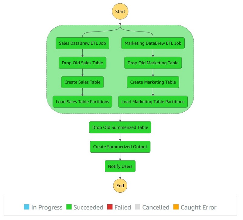
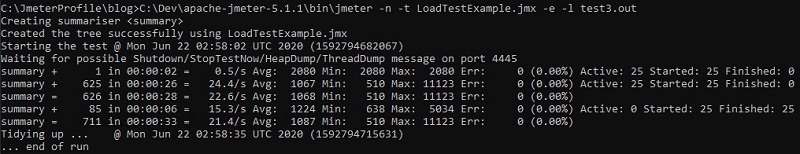
If you scroll down, you should see an ExecutionSucceeded message in the last line of the event history (see the following screenshot).

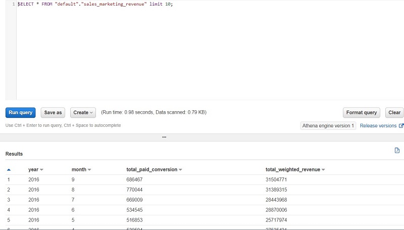
- On the Amazon S3 console, search for the bucket name used in this post (hudiblog-[account-id]) and then for the prefix
raw/multitenant/salesdb/sales_order_detail_mt/.
You should see two files.
- Navigate to the prefix
transformed/multitenant/salesdb/sales_order_detail_mt/.
You should see the Hudi table Parquet format.
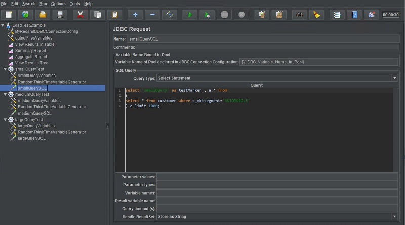
Analyzing the properties provided to the command to run the Hudi DeltaStreamer utility
If the MultitenantProcessing workflow was successful, the files that AWS DMS loaded into Amazon S3 are now available in a multi-tenant table on Amazon S3. This table is now ready to process changes to the databases for each tenant.
In this step, we go over the command the workflow triggers to create a table with Hudi.
The Step Functions workflow for this post runs all the steps except the tasks in the Amazon Sagemaker notebook that you trigger. The following section is just for your reference and discussion purposes.
On the Amazon EMR console, choose the cluster created by the CloudFormation and choose the Steps view of the cluster to obtain the full command used by the workflow.

The command has two sets of properties: one defined directly in the command, and another defined on a configuration file, dfs-source.properties, which is updated automatically by the Step Functions workflow.
The following are some of the properties defined directly in the command:
- –table-type – The Hudi table type, for this use case,
COPY_ON_WRITE. The reason COPY_ON_WRITE is preferred for this use case relates to the fact that the ingestion is done in batch mode, access to the changes in the data are not required in real time, and the downstream workloads are read-heavy. Moreover, with this storage type, you don’t need to handle compactions because updates create a new Parquet file with the impacted rows being updated. Given that the ingestion is done in batch mode, using the COPY_ON_WRITE table type efficiently keeps track of the latest record change, triggering a new write to update the Hudi dataset with the latest value of the record.
- This post requires that you use the
COPY_ON_WRITE table type.
- For reference, if your requirement is to ingest write- or change-heavy workloads and make the changes available as fast as possible for downstream consumption, Hudi provides the
MERGE_ON_READ table type. In this table type, data is stored using a combination of columnar (Parquet) and row-based (Avro) formats. Updates are logged to row-based delta files and are compacted as needed to create new versions of the columnar files. For more details on the two table types provided by Hudi, see Understanding Dataset Storage Types: Copy on Write vs. Merge on Read and Considerations and Limitations for Using Hudi on Amazon EMR.
- –source-ordering-field – The field in the source dataset that the utility uses to order the records. For this use case, we configured AWS DMS to add a
timestamp column to the data. The utility uses that column to order the records and break ties between records with the same key. This field needs to exist in the data source and can’t be the result of a transformation.
- –source-class – AWS DMS writes to the Amazon S3 destination in Apache Parquet. Use
apache.hudi.utilities.sources.ParquetDFSSource as the value for this property.
- –target-base-path – The destination base path that the utility writes.
- –target-table – The table name of the table the utility writes to.
- –transformer-class – This property indicates the transformer classes that the utility is applied to the input records. For this use case, we use the
AWSDmsTransformer plus the SqlQueryBasedTransformer. The transformers are applied in the order they are identified in this property.
- –payload-class – Set to
org.apache.hudi.payload.AWSDmsAvroPayload.
- –props – The path of the file with additional configurations. For example,
file:///home/hadoop/dfs-source.properties.
- The file /home/hadoop/dfs-source.properties has additional configurations passed to Hudi DeltaStreamer. You can view that file by logging in to your Amazon EMR master node and running
cat /home/hadoop/dfs-source.properties.
The following code is the configuration file. By setting the properties in the file, we configure Hudi to write the dataset in a partitioned way and applying a SQL transform before persisting the dataset into the Amazon S3 location.
===Start of Configuration File ===
hoodie.datasource.write.keygenerator.class=org.apache.hudi.keygen.ComplexKeyGenerator
hoodie.datasource.write.partitionpath.field=tenant_id,year,month
hoodie.deltastreamer.transformer.sql=SELECT a.timestamp, a.line_id, a.line_number, a.order_id, a.product_id,  a.quantity, a.unit_price, a.discount, a.supply_cost, a.tax, string(year(to_date(a.order_date))) as year, string(month(to_date(a.order_date))) as month, a.Op, a.tenant_id FROM <SRC> a
hoodie.datasource.write.recordkey.field=tenant_id,line_id
hoodie.datasource.write.hive_style_partitioning=true
# DFS Source
hoodie.deltastreamer.source.dfs.root=s3://hudiblog-xxxxxxxxxxxxxx/raw/multitenant/salesdb/sales_order_detail_mt/xxxxxxxxxxxxxxxxxxxxx
===End of Configuration File ===
Some configurations in this file include the following:
- hoodie.datasource.write.operation=upsert – This property defines if the write operation is an insert, upsert, or
bulkinsert. If you have a large initial import, use bulkinsert to load new data into a table, and on the next loads use upsert or insert. The default value for this property is upsert. For this post, the default is accepted because the dataset is small. When you run the solution with larger datasets, you can perform the initial import with bulkinsert and then use upsert for the next loads. For more details on the three modes, see Write Operations.
- hoodie.datasource.write.hive_style_partitioning=true – This property generates Hive style partitioning—partitions of the form
partition_key=partition_values. See the property hoodie.datasource.write.partitionpath.field for more details.
- hoodie.datasource.write.partitionpath.field=tenant_id,year,month – This property identifies the fields that Hudi uses to extract the partition fields.
- hoodie.datasource.write.keygenerator.class=org.apache.hudi.keygen.ComplexKeyGenerator – This property allows you to combine multiple fields and use the combination of fields as the record key and partition key.
- hoodie.datasource.write.recordkey.field=tenant_id,line_id – This property indicates the fields in the dataset that Hudi uses to identify a record key. The source table has
line_id as the primary key. Given that the Hudi dataset is multi-tenant, tenant_id is also part of the record key.
- hoodie.deltastreamer.source.dfs.root=s3://hudiblog-your-account-id/raw/multitenant/salesdb/sales_order_detail_mt/xxxxxxxxx – This property indicates the Amazon S3 location with the source files that the Hudi DeltaStreamer utility consumes. This is the location that the
MultiTenantProcessing state machine created and includes files from both tenants.
- hoodie.deltastreamer.transformer.sql=SELECT a.timestamp, a.line_id, a.line_number, a.order_id, a.product_id, a.quantity, a.unit_price, a.discount, a.supply_cost, a.tax, year(string(a.order_date)) as year, month(string(a.order_date)) as month, a.Op, a.tenant_id FROM a – This property indicates that the Hudi DeltaStreamer applies a SQL transform before writing the records as a Hudi dataset in Amazon S3. For this use case, we create new fields from the RBDMS table’s field
order_date.
A change to the schema of the source RDBMS tables requires the respective update to the SQL transformations. As mentioned before, this use case requires that schema changes to a source schema occur in every table for every tenant.
For additional details on Hudi, see Apply record level changes from relational databases to Amazon S3 data lake using Hudi on Amazon EMR and AWS DMS.
Although the Hudi multi-tenant table is partitioned, you should only have one job (Hudi DeltaStreamer utility or Spark data source) writing to the Hudi dataset. If you’re expecting specific tenants to produce more changes than others, you can consider prioritizing some tenants over others or use dedicated tables for the most active tenants to avoid any impact to tenants that produce a smaller amount of changes.
Schema evolution
Hudi supports schema evolutions that are backward compatible—you only append new fields and don’t delete any existing fields.
By default, Hudi handles schema changes of type by appending new fields to the end of the table.
New fields that you add have to either be nullable or have a default value. For example, as you add a new field to the source database, the records that generate a change have a value for that field in the Hudi dataset, but older records have a null value for that same field in the dataset.
If you require schema changes that are not supported by Hudi, you need to use either a SQL transform or the Hudi DataSource API to handle those changes before writing to the Hudi dataset. For example, if you need to delete a field from the source, you need to use a SQL transform before writing the Hudi dataset to ensure the deleted column is populated by a constant or dummy value, or use the Hudi DataSource API to do so.
Moreover, AWS DMS with Amazon S3 targets support only the following DDL commands: Truncate Table, Drop Table, and Create Table. See Limitations to using Amazon S3 as a target for more details.
This means that when you issue an Alter Table command, the AWS DMS replication tasks don’t capture those changes until you restart the task.
As you implement this architecture pattern, it’s recommended that you automate the schema evolution process and apply the schema changes in a maintenance window when the source isn’t serving requests and the AWS DMS replication CDC tasks aren’t running.
Simulating random updates to the source databases
In this step, you perform some random updates to the data. Navigate back to the Runmev5.ipynb Jupyter notebook and run the cells under the section Simulate random updates for tenant 1 and tenant 2.
Triggering the Step Functions workflow to process the ongoing replication
In this step, you rerun the MultitenantProcessing workflow to process the files generated during the ongoing replication.
- On the Step Functions console, choose State machines.
- Choose the
MultiTenantProcessing workflow
- In the new window, choose Start execution.
- Use the same JSON as the JSON used when you first ran the workflow.
- Submit the edited JSON as the input to the workflow.
Querying the Hudi multi-tenant table with Spark
To query your table with Spark, complete the following steps:
- On the Session Manager console, select the instance HudiBlog Spark EMR Cluster.
- Choose Start session.

Session Manager creates a secure session to the Amazon EMR master node.
- Switch to the Hadoop user and then to the home directory of the Hadoop user.

You’re now ready to run the commands described in the next sections.
- Run the following command in the command line:
spark-shell --conf "spark.serializer=org.apache.spark.serializer.KryoSerializer" --conf "spark.sql.hive.convertMetastoreParquet=false" --jars /usr/lib/hudi/hudi-spark-bundle.jar,/usr/lib/spark/external/lib/spark-avro.jar
- When the spark-shell is available, enter the following code:
import scala.collection.JavaConversions._
import org.apache.spark.sql.SaveMode._
import org.apache.hudi.DataSourceReadOptions._

val tableName = "sales_order_detail_mt"

val basePath = "s3://hudiblog-[REPLACE-WITH-YOUR-ACCOUNT-ID]/transformed/multitenant/huditables/"+tableName+"/"

spark.read.format("org.apache.hudi").load(basePath + "/*/*/*/*").createOrReplaceTempView(tableName)

val sqlDF = spark.sql("SELECT * FROM "+tableName)
sqlDF.show(20,false)
Updating the source table schema
In this section, you change the schema of the source tables.
- On the AWS DMS management console, stop the AWS DMS replication tasks for Tenant 1 and Tenant 2.
- Make sure the Amazon SageMaker notebook isn’t writing to the database.
- Navigate back to the Jupyter notebook and run the cells under the section Updating the source table schema.
- On the AWS DMS console, resume (not restart) the AWS DMS replication tasks for both tenants.
- Navigate back to the Jupyter notebook and run the cells under the section Simulate random updates for tenant 1 after the schema change.
Analyzing the changes to the configuration file for the Hudi DeltaStreamer utility
Because there was a change to the schema of the sources and a new field needs to be propagated to the Hudi dataset, the property hoodie.deltastreamer.transformer.sql is updated with the following value:
hoodie.deltastreamer.transformer.sql=SELECT a.timestamp, a.line_id, a.line_number, a.order_id, a.product_id, a.quantity, a.unit_price, a.discount, a.supply_cost, a.tax, string(year(to_date(a.order_date))) as year, string(month(to_date(a.order_date))) as month, a.Op, a.tenant_id, a.critical FROM <SRC> a
The field a.critical is added to the end, after a.tenant_id.
Triggering the Step Functions workflow to process the ongoing replication after the schema change
In this step, you rerun the MultitenantProcessing workflow to process the files produced by AWS DMS during the ongoing replication.
- On the Step Functions console, choose State machines.
- Choose the
MultiTenantProcessing
- In the new window, choose Start execution.
- Update the JSON document used when you first ran the workflow by replacing the field
propertiesFilename with the following value:
"propertiesFilename": "dfs-source-new_schema.properties"
- Submit the edited JSON as the input to the workflow.
Querying the Hudi multi-tenant table after the schema change
We can now query the multi-tenant table again.
Using Hive
If using Hive when the workflow completes, go back to the terminal window opened by Session Manager and run the following hive-sync command:
/usr/lib/hudi/bin/run_sync_tool.sh --table sales_order_detail_mt --partitioned-by tenant_id,year,month --database default --base-path s3://hudiblog-[REPLACE-WITH-YOUR-ACCOUNT-ID]/transformed/multitenant/huditables/sales_order_detail_mt --jdbc-url jdbc:hive2:\/\/localhost:10000 --user hive --partition-value-extractor org.apache.hudi.hive.MultiPartKeysValueExtractor --pass passnotenforced
For this post, we run the hive-sync command manually. You can also add the flag --enable-hive-sync to the Hudi DeltaStreamer utility command showed in section Analyzing the properties provided to the command to run the Hudi DeltaStreamer utility.
After the hive-sync updates the table schema, the new column is visible from Hive. Start Hive in the command line and run the following query:
select `timestamp`, quantity, critical, order_id, tenant_id from sales_order_detail_mt where order_id=4668 and tenant_id=1502;
Using Spark
If you just want to use Spark to read the Hudi datasets on Amazon S3, after the schema change, you can use the same code in Querying the Hudi multi-tenant table with Spark and add the following line to the code:
spark.conf.set("spark.sql.parquet.mergeSchema", "true")
Cleaning up
To avoid incurring future charges, stop the AWS DMS replication tasks, delete the contents in the S3 bucket for the solution, and delete the CloudFormation stack.
Conclusion
This post explained how to use AWS DMS, Step Functions, and Hudi on Amazon EMR to convert a single-tenant pipeline to a multi-tenant pipeline.
With this solution, your software offerings that use dedicate sources for each tenant can offload some of the common tasks across all the tenants to a pipeline backed by Hudi datasets stored on Amazon S3. Moreover, by using Hudi on Amazon EMR, you can easily apply inserts, updates, and deletes of the source databases to the datasets in Amazon S3. Moreover, you can easily support schema evolution that is backward compatible.
Follow these steps and deploy the CloudFormation templates in your account to further explore the solution. If you have any questions or feedback, please leave a comment.
The author would like to thank Radhika Ravirala and Neil Mukerje for the dataset and the functions on the notebook.
About the Author
 Francisco Oliveira is a senior big data solutions architect with AWS. He focuses on building big data solutions with open source technology and AWS. In his free time, he likes to try new sports, travel and explore national parks.
 Cristian Gavazzeni is a senior solution architect at Amazon Web Services. He has more than 20 years of experience as a pre-sales consultant focusing on Data Management, Infrastructure and Security. During his spare time he likes eating Japanese food and travelling abroad with only fly and drive bookings.
 Francesco Marelli is a senior solutions architect at Amazon Web Services. He has lived and worked in London for 10 years, after that he has worked in Italy, Switzerland and other countries in EMEA. He is specialized in the design and implementation of Analytics, Data Management and Big Data systems, mainly for Enterprise and FSI customers. Francesco also has a strong experience in systems integration and design and implementation of web applications. He loves sharing his professional knowledge, collecting vinyl records and playing bass.


 Al MS is a product manager for Amazon EMR at Amazon Web Services.
 Peter Gvozdjak is a senior engineering manager for EMR at Amazon Web Services.


 Sai Sriparasa is a Sr. Big Data & Security Consultant with AWS Professional Services. He works with our customers to provide strategic and tactical big data solutions with an emphasis on automation, operations, governance & security on AWS. In his spare time, he follows sports and current affairs.
 Ravi Kadiri is a security data architect at AWS, focused on helping customers build secure data lake solutions using native AWS security services. He enjoys using his experience as a Big Data architect to provide guidance and technical expertise on Big Data & Analytics space. His interests include staying fit, traveling and spend time with friends & family.


 Dipankar Ghosal is a Sr Data Architect at Amazon Web Services and is based out of Minneapolis, MN. He has a focus in analytics and enjoys helping customers solve their unique use cases. When he’s not working, he loves going hiking with his wife and daughter.


 Varun Rao Bhamidimarri is a Sr Manager, AWS Analytics Specialist Solutions Architect team. His focus is helping customers with adoption of cloud-enabled analytics solutions to meet their business requirements. Outside of work, he loves spending time with his wife and two kids, stay healthy, mediate and recently picked up garnering during the lockdown.


 Arash Rowshan is a Software Engineer at Amazon Web Services. He’s passionate about big data and applications of ML. Most recently he was part of the team that launched AWS Glue DataBrew. Any time he’s not at his desk, he’s likely playing soccer somewhere. You can follow him on Twitter
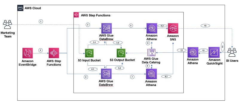


 Saurabh Shrivastava is a solutions architect leader and analytics/machine learning specialist working with global systems integrators. He works with AWS partners and customers to provide them with architectural guidance for building scalable architecture in hybrid and AWS environments. He enjoys spending time with his family outdoors and traveling to new destinations to discover new cultures.
 Sameer Goel is a solutions architect in Seattle who drives customers’ success by building prototypes on cutting-edge initiatives. Prior to joining AWS, Sameer graduated with a Master’s degree with a Data Science concentration from NEU Boston. He enjoys building and experimenting with creative projects and applications.
 Pratik Patel is a senior technical account manager and streaming analytics specialist. He works with AWS customers and provides ongoing support and technical guidance to help plan and build solutions by using best practices, and proactively helps keep customers’ AWS environments operationally healthy.


 Saurabh Bhutyani is a Senior Big Data Specialist Solutions Architect at Amazon Web Services. He is an early adopter of open-source big data technologies. At AWS, he works with customers to provide architectural guidance for running analytics solutions on Amazon EMR, Amazon Athena, AWS Glue, and AWS Lake Formation. In his free time, he likes to watch movies and spend time with his family.
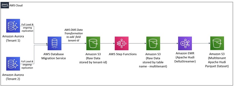


 Francisco Oliveira is a senior big data solutions architect with AWS. He focuses on building big data solutions with open source technology and AWS. In his free time, he likes to try new sports, travel and explore national parks.
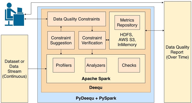
 Calvin Wang is a Data Scientist at AWS AI/ML. He holds a B.S. in Computer Science from UC Santa Barbara and loves using machine learning to build cool stuff.
 Chris Ghyzel is a Data Engineer for AWS Professional Services. Currently, he is working with customers to integrate machine learning solutions on AWS into their production pipelines.
 Veronika Megler, PhD, is Principal Data Scientist for Amazon.com Consumer Packaging. Until recently she was the Principal Data Scientist for AWS Professional Services. She enjoys adapting innovative big data, AI, and ML technologies to help companies solve new problems, and to solve old problems more efficiently and effectively. Her work has lately been focused more heavily on economic impacts of ML models and exploring causality.


 Seetha Sarma is a Senior Database Specialist Solutions Architect with Amazon Web Services. Seetha provides guidance to customers on using AWS services for distributed data processing. In her spare time she likes to go on long walks and enjoy nature.
 Moiz Mian is a Solutions Architect for AWS Strategic Accounts. He focuses on enabling customers to build innovative, scalable, and secure solutions for the cloud. In his free time, he enjoys building out Smart Home systems and driving at race tracks.


 Shilpa Mohan is a Sr. UX designer at AWS and leads the design of AWS Glue DataBrew. With over 13 years of experience across multiple enterprise domains, she is currently crafting products for Database, Analytics and AI services for AWS. Shilpa is a passionate creator, she spends her time creating anything from content, photographs to crafts
 Romi Boimer is a Sr. Software Development Engineer at AWS and a technical lead for AWS Glue DataBrew. She designs and builds solutions that enable customers to efficiently prepare and manage their data. Romi has a passion for aerial arts, in her spare time she enjoys fighting gravity and hanging from fabric.


 Sain Das is an Analytics Specialist Solutions Architect at AWS and helps customers build scalable cloud solutions that help turn data into actionable insights.
 Vijetha Parampally Vijayakumar is a full stack software development engineer with Amazon Redshift. She is specialized in building applications for Big data, Databases and Analytics.
 André Dias is a Systems Development Engineer working in the Amazon Redshift team. André’s passionate about learning and building new AWS Services and has worked in the Redshift Data API. He specializes in building highly available and cost-effective infrastructure using AWS.


 Asser Moustafa is an Analytics Specialist Solutions Architect at AWS based out of Dallas, Texas. He advises customers in the Americas on their Amazon Redshift and data lake architectures and migrations, starting from the POC stage to actual production deployment and maintenance


 Harsha Tadiparthi is a Specialist Sr. Solutions Architect, AWS Analytics. He enjoys solving complex customer problems in Databases and Analytics and delivering successful outcomes. Outside of work, he loves to spend time with his family, watch movies, and travel whenever possible.
 Harshida Patel is a Specialist Sr. Solutions Architect, Analytics with AWS.