Agentic application modernization at scale with Strands and Amazon Transform custom

Post Syndicated from Kanishk Mahajan original https://aws.amazon.com/blogs/devops/use-generative-ai-agents-for-application-modernization-at-scale-with-strands-amazon-transform-custom-and-amazon-bedrock-agentcore/

Introduction

Modernizing applications by upgrading language runtimes, migrating SDKs, and refactoring frameworks is important for cloud adoption but can be labor-intensive at scale. Each repository requires analysis of dependencies and transformation needs; custom transformation logic must be built and validated, and changes are often executed sequentially across codebases. If you have hundreds of applications, this stretches timelines from months to years, while introducing inconsistency across your teams.

To address this, Amazon Web Services (AWS) provides a composable set of building blocks. AWS Transform custom enables reusable, CLI-driven code transformations for upgrading runtimes, SDKs, and frameworks consistently across large portfolios. Strands Agents provides a framework for building multi-agent systems that coordinate complex transformation workflows. Amazon Bedrock AgentCore delivers the managed runtime, memory, and observability to operate these agents reliably in production. Together, they replace manual, sequential modernization with an intelligent, automated approach that scales.

In this post, we show you how to combine these services to build a generative AI–powered, agentic modernization system that can automatically analyze application repositories, determine required changes, create missing transformations, and execute them in parallel at scale.

Solution overview

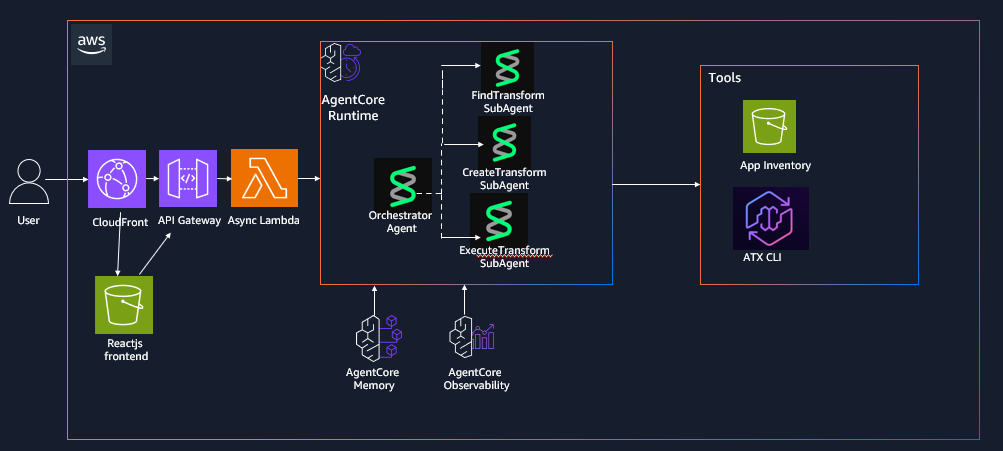
The solution uses an agentic architecture that separates intelligent decision-making from deterministic execution, enabling automation at scale while maintaining consistency and control. In this post, you will build an AI-driven application modernization system that demonstrates how multi-agent workflows can be applied to large-scale code transformation scenarios. You interact with the system through a React-based frontend or API interface, submitting individual repositories or batch workloads via CSV inputs. Requests are processed asynchronously through an API layer that invokes an orchestrator agent running on Amazon Bedrock AgentCore, which coordinates specialized agents to analyze codebases, identify transformation requirements, and manage execution workflows. Results are stored and surfaced through the interface, allowing users to track progress and review outputs in real time.The workflow begins with repository analysis, where the system inspects application codebases to identify languages, dependencies, and required upgrades such as runtime version changes or SDK migrations. Based on this analysis, the system maps each application to an existing transformation when available. If no suitable transformation exists, a creation agent dynamically generates one using natural language instructions and publishes it to a centralized registry for reuse, creating a continuously improving system where transformation coverage expands over time.

Once transformations are identified or created, an execution agent runs them at scale by invoking AWS Batch jobs that execute the AWS Transform custom CLI, enabling parallel processing across multiple repositories. The orchestrator coordinates all agents, maintains workflow state using Amazon Bedrock AgentCore Memory, and ensures reliable execution through structured task decomposition, tool invocation, and error handling. While the example focuses on application re-platforming, the same architectural pattern can be applied to other large-scale code analysis and automation workflows.

The following architecture diagram (Figure 1) illustrates the various components of our solution as outlined in this section:architecture diagram describing the multi agent strands and agentcore deployment

Figure 1: AWS Transform custom Agentic Orchestration Architecture using Strands agents and Amazon Bedrock AgentCore

Prerequisites

Complete the following prerequisites:

  1. Install the AWS Command Line Interface (AWS CLI).
  2. Install the AWS SAM CLI v1.100.0+
  3. Install Docker v20.x+.
  4. Install Node.js v18.x+
  5. Install Python v3.11+
  6. Install the AWS CDK CLI
  7. Enable access to a Bedrock model for the orchestrator in your deployment region. The default model can be configured through the Amazon Bedrock model access console. To use a different model, set `BEDROCK_MODEL_ID` in `deployment/config.env` before Step 3 and enable access to that model instead. Model access approval can take a few minutes in some accounts, so complete this step before deploying.

Dependencies

The Strands Agents implementation has the following dependencies that are packaged in the DockerFile:

  1. Strands multi-agent framework: strands-agents
  2. Strands agent tools and utilities: strands-agents-tools
  3. HTTP library for API calls: requests
  4. Amazon Bedrock AgentCore SDK: bedrock-agentcore
  5. AWS SDK for Python: boto3

Deploy the solution

The solution is available for download on the GitHub repo. This post walks through the CDK + SAM deployment path (Option A in the repository README). The repository also includes a CDK-only option (Option B); see the repository README for details.

Step 1: Clone the repository

git clone https://github.com/aws-samples/aws-transform-custom-samples.git

cd aws-transform-custom-samples/agentic-atx-platform

Step 2: Configure AWS Credentials

# Configure AWS CLI

aws configure

# Verify credentials

aws sts get-caller-identity

Step 3: Deploy ATX CLI Container image and frontend using AWS CDK

# Copy configuration template (defaults work for most setups; edit only to change region or Bedrock model)

cd deployment

cp config.env.template config.env

# Authenticate with Amazon ECR Public (required for the Docker base image pull)

aws ecr-public get-login-password --region us-east-1 | docker login --username AWS --password-stdin public.ecr.aws

# Build the UI placeholder so CDK’s UI stack has ui/dist/ to deploy

cd ../ui && npm install && npx vite build

# Install CDK dependencies and bootstrap (run once per account/region)

cd ../cdk

npm install cdk bootstrap

# Build TypeScript and deploy the three stacks

npx tsc

CDK_DEFAULT_ACCOUNT=$(aws sts get-caller-identity --query Account --output text)

cdk deploy AtxContainerStack AtxInfrastructureStack AtxUiStack --require-approval never

# Note for accounts without a default VPC , pass the VPC context flags to `cdk deploy`:

cdk deploy AtxContainerStack AtxInfrastructureStack AtxUiStack --require-approval never

cdk deploy AtxContainerStack AtxInfrastructureStack AtxUiStack --require-approval never -c existingVpcId=vpc-xxx -c existingSubnetIds=subnet-aaa,subnet-bbb -c existingSecurityGroupId=sg-ccc

# Subnets must be public (auto-assign public IP enabled) or private with a NAT gateway so Fargate tasks can reach Amazon ECR, Amazon S3, and Git repositories.

Step 4: Deploy Strands Agents to AgentCore runtime using AWS SAM

cd ../sam./deploy.sh

# Invoke the deploy Lambda to create the AgentCore Runtime via the bedrock-agentcore-control SDK (takes 2-5 minutes)

aws lambda invoke --function-name atx-deploy-agentcore \ --region us-east-1 \ --cli-binary-format raw-in-base64-out \ --payload '{"action":"deploy"}' \ --cli-read-timeout 900 /tmp/deploy-output.jsoncat /tmp/deploy-output.json

Step 5: Wire the AgentCore runtime ARN into the async invoke Lambda

ACCOUNT_ID=$(aws sts get-caller-identity --query Account --output text)

RUNTIME_ARN=$(python3 -c "import json; print(json.loads(json.load(open('/tmp/deploy-output.json'))['body'])['runtime_arn'])")aws lambda update-function-configuration \ --function-name atx-async-invoke-agent \ --region us-east-1 \ --environment "Variables={AGENT_RUNTIME_ARN=${RUNTIME_ARN},RESULT_BUCKET=atx-custom-output-${ACCOUNT_ID},JOBS_TABLE=atx-transform-jobs}"

Step 6: Rebuild and deploy the frontend with AgentCore API endpoint

# Update the React application with the deployed API endpoint and redeploy it.

API_URL=$(aws cloudformation describe-stacks \ --stack-name AtxAgentCoreSAM \ --region us-east-1 \ --query 'Stacks[0].Outputs[?OutputKey==`ApiEndpoint`].OutputValue' \ --output text)

cd ../ui

VITE_API_ENDPOINT=$API_URL npx vite build./deploy-aws.sh

# This rebuilds the React application with the correct API endpoint, uploads it to Amazon S3, and invalidates the Amazon CloudFront distribution.

Step 7: Access the application

# After deployment completes, retrieve the CloudFront distribution URL from the AWS CloudFormation outputs and open it in your browser to access the application UI.

aws cloudformation describe-stacks \ --stack-name AtxUiStack \ --region us-east-1 \ --query 'Stacks[0].Outputs[?OutputKey==`WebsiteUrl`].OutputValue' \ --output text

Using the application

The UI exposes five tabs covering the complete modernization workflow: browsing available transformations, executing a transformation on a single repository, creating a new custom transformation with natural language, batch-processing a CSV of repositories, and tracking job status. This section walks through two of the most common flows.

Create a custom transformation from natural language

Open the Create Custom tab, describe the transformation in plain English (for example, “Upgrade Spring Boot 2 applications to Spring Boot 3”), and optionally provide a reference repository URL. The creation agent analyzes the source, generates a transformation definition, and publishes it to the ATX registry for reuse across the portfolio.

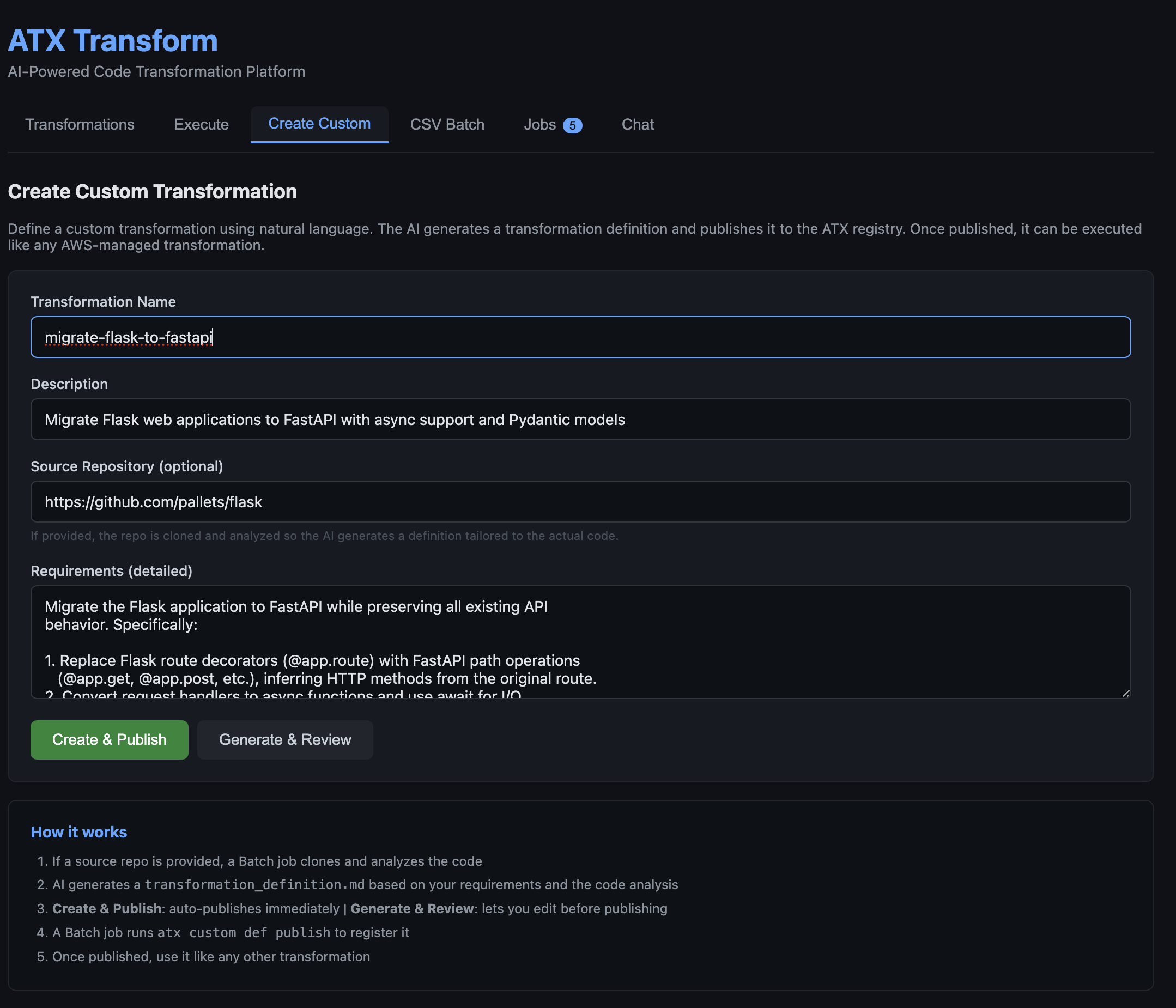
Describing a custom transformation in plain English. The form accepts a name, description, optional reference repository, and natural-language requirements.

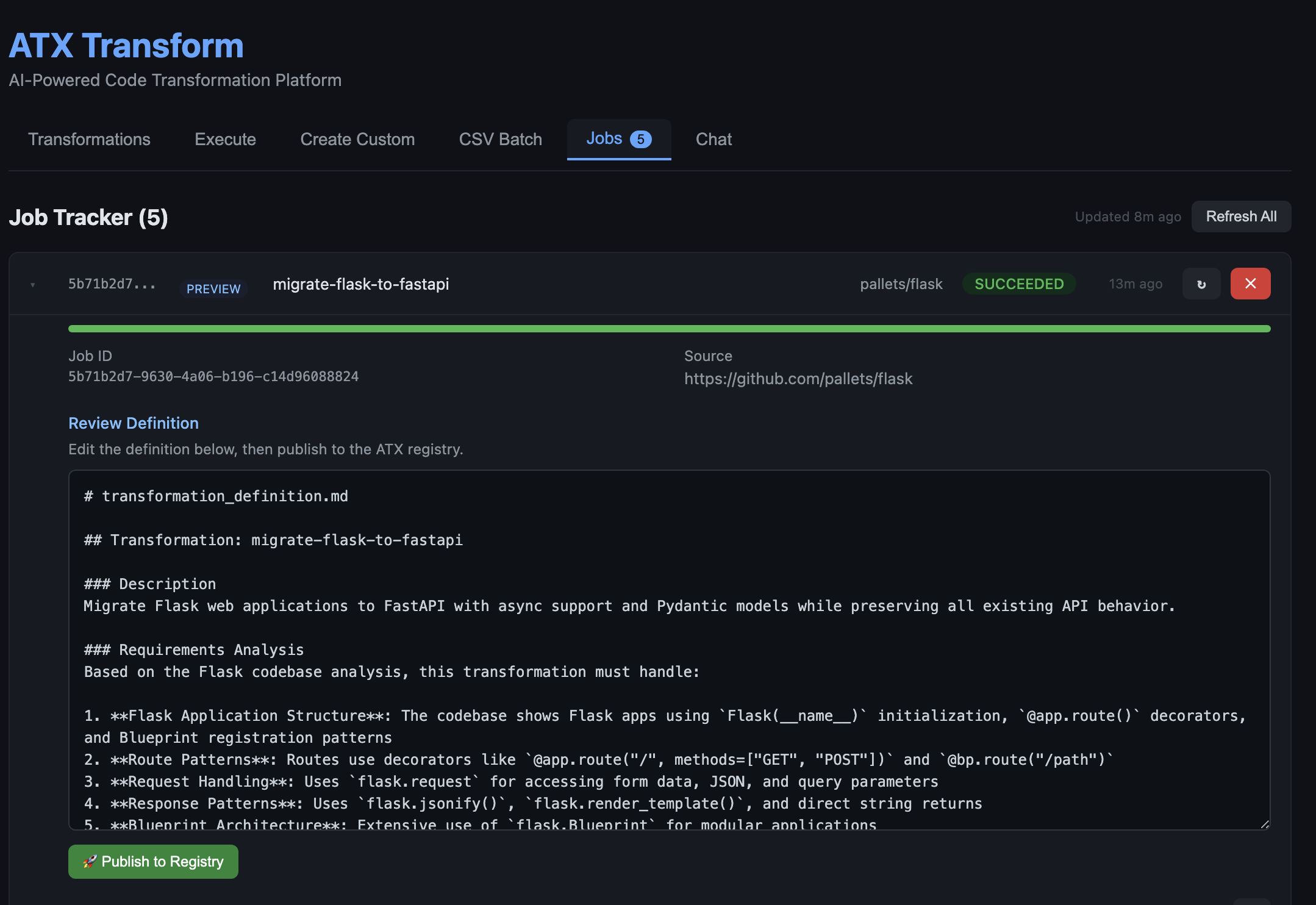
Figure 2: Describing a custom transformation in plain English. The form accepts a name, description, optional reference repository, and natural-language requirements.After submitting, the orchestrator clones the reference repository, analyzes the source, and generates a transformation definition tailored to the actual code patterns found in the codebase. This takes 1–5 minutes depending on repository size. The generated definition is then shown for review in the Jobs tab, where it can be edited before publishing to the ATX registry.

Figure 3: The AI-generated transformation definition shown for review in the Jobs tab. The agent analyzed the Flask codebase and produced a detailed definition covering routes, request handling, response patterns, and Blueprint architecture. The user can edit the definition in-place and click Publish to Registry when ready.Once published, the new transformation appears in the Transformations tab alongside AWS-managed transformations and can be executed the same way on any repository.

Run a batch of repositories from a CSV

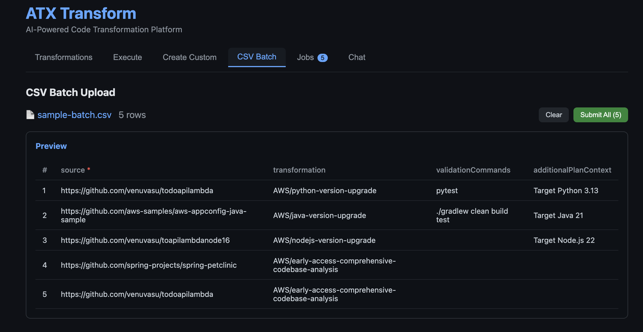
Open the CSV Batch tab and upload a CSV listing repository URLs and target transformations. A sample `sample-batch.csv` is included in the repository at `agentic-atx-platform/ui/sample-batch.csv`. The preview shows the parsed rows before submission. On Submit All, each row becomes a separate AWS Batch job running in parallel, and the Jobs tab shows live status as repositories complete.

Uploading a batch of repositories for parallel processing. The CSV lists a source repository URL, target transformation, optional validation commands, and additional plan context per row.

Figure 4: Uploading a batch of repositories for parallel processing. The CSV lists a source repository URL, target transformation, optional validation commands, and additional plan context per row. Each row becomes an independent AWS Batch job on submission.

Clean up

To avoid recurring charges, remove the resources after trying the solution.

Step 1: Delete the SAM Stack

sam delete --stack-name AtxAgentCoreSAM --region us-east-1 --no-prompts

Step 2: Delete the CDK Stacks

Remove the three CDK stacks in reverse order. The S3 buckets are configured with `autoDeleteObjects: true`, so CDK will empty them before deletion.

cd cdk

npx cdk destroy AtxUiStack AtxInfrastructureStack AtxContainerStack --force

Conclusion

In this post, you learned how to build a generative AI–powered, agentic system for application modernization that can analyze application repositories, determine required code changes, create missing transformations, and execute those transformations at scale. By combining AWS Transform Custom for transformation execution with Amazon Bedrock AgentCore for orchestration, and Strands Agents for multi-agent coordination and AWS Transform container solution for parallel processing, this approach demonstrates how intelligent automation can be applied to large-scale code transformation workflows.

This solution directly addresses the challenges of traditional modernization approaches. It reduces manual effort by automating repository analysis and transformation mapping, eliminates gaps in transformation coverage by dynamically generating reusable transformations, and significantly improves scalability through parallel execution using AWS Batch.

By introducing a centralized, agent-driven workflow with built-in observability and state management, organizations can achieve faster, more consistent, and governed modernization across large application portfolios. To get started, deploy the solution in your AWS environment, test it with a sample repository or batch workload, and extend it by creating custom transformations tailored to your applications. You can further integrate this approach into your CI/CD pipelines to enable continuous modernization and accelerate your cloud migration initiatives.


About the authors

Kanishk Mahajan is Principal – AI/ML with AWS Professional Services. In this role, he leads GenAI and agentic transformations for some of AWS largest customers in Telco and Media & Entertaintment.

Sandeep Batchu is a Senior Security Architect at Amazon Web Services, with extensive experience in software engineering, solutions architecture, and cybersecurity. Passionate about bridging business outcomes with technological innovation, Sandeep guides customers through their cloud and generative AI journey, helping them design and implement secure, scalable, and resilient architectures in the era of AI-driven transformation.

Venugopalan Vasudeven (Venu) is a Principal Specialist Solutions Architect at AWS, where he leads Agentic AI initiatives focused on AWS Transform. He helps customers adopt and scale AI-powered developer and modernization solutions to accelerate innovation and business outcomes.
How to use streamlined permissions for Amazon S3 Tables and Iceberg materialized views

Post Syndicated from Srividya Parthasarathy original https://aws.amazon.com/blogs/big-data/how-to-use-streamlined-permissions-for-amazon-s3-tables-and-iceberg-materialized-views/

Apache Iceberg has emerged as the open table format for data lakes. It handles petabyte-scale datasets, lets teams evolve schemas and partitions in place, and supports time travel and incremental processing for data lake management at scale. Amazon S3 Tables provide a fully managed Apache Iceberg table experience in Amazon S3, optimized for analytics workloads, and integrate with the AWS Glue Data Catalog so AWS analytics services such as Amazon Redshift, Amazon EMR, Amazon Athena, Amazon SageMaker, and AWS Glue query your data. Together, they form the foundation of a modern data lake architecture on AWS.

S3 Tables integrate with the AWS Glue Data Catalog using AWS Identity and Access Management (IAM) – based authorization. If you manage analytics workloads across these services, you can now define permissions across storage, catalog, and compute in a single IAM policy. This gives teams already using IAM a straightforward path to govern access to S3 Tables resources without changing their existing permission model. For fine-grained access controls, you can opt in to AWS Lake Formation at any time through the AWS Management Console, AWS Command Line Interface (AWS CLI), API, or AWS CloudFormation.

Iceberg materialized views created in the Glue Data Catalog extend this foundation by letting you store pre-computed query results as Iceberg data on Amazon S3. When a query repeats aggregations or joins across large datasets, the engine reads directly from the materialized view’s S3 location rather than reprocessing the base tables. A materialized view can reside in S3 Tables or in an S3 general purpose bucket, independent of where its base tables live, which lets you place pre-computed results wherever fits your access patterns and cost model best.

In this post, we walk through how to set up and manage S3 Tables in the AWS Glue Data Catalog, create and query Iceberg materialized views, and configure access controls that work across your analytics stack with IAM-based authorization.

 Solution overview

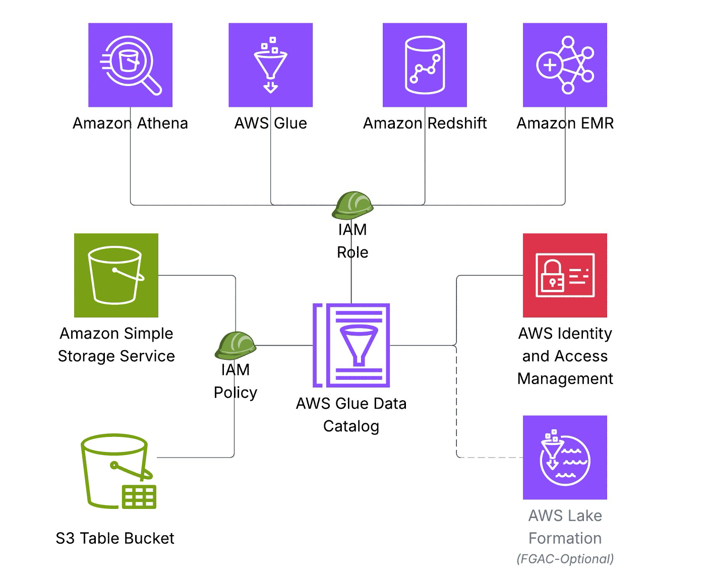
Architecture diagram showing AWS Glue Data Catalog integration with Amazon Athena, AWS Glue, Amazon Redshift, and Amazon EMR through IAM roles and policies, with Amazon S3 storage and optional AWS Lake Formation governance.

The above architecture illustrates how S3 Tables integrate with AWS Glue Data Catalog using IAM-based authorization, so you can define the necessary permissions across storage, catalog, and query engines in a single IAM policy. This permission model accelerates onboarding for new teams and workloads.

Key architecture components include:

Storage Layer: Data stored as Iceberg tables in Amazon S3 Tables

Catalog Layer: AWS Glue Data Catalog serves as the single metadata repository.

Compute Layer – Amazon Athena, AWS Glue, Amazon Redshift, and Amazon EMR connect to a single data Catalog to access Iceberg tables.

Security: AWS IAM authorizes access to resources in storage, catalog, and compute layers.

Prerequisites:

To follow along with this post, you must have an AWS account and an IAM role or user with appropriate permissions and familiarity to the following services:

  • IAM
  • AWS Glue Data Catalog
  • Amazon S3
  • Amazon Athena
  • Amazon Redshift
  • Amazon EMR

For the minimum permissions required for the role/user for metadata and data access, refer to required IAM permissions documentation.

Solution walkthrough

In this walkthrough, you will integrate S3 Tables with the AWS Glue Data Catalog, create Iceberg materialized views, and query data using multiple analytics engines. You will also learn to use materialized views when you have complex aggregations queried frequently but underlying data changes. You can follow these steps to implement the solution. It will take about 45–60 minutes to complete this walkthrough.

Setup S3 Tables and integrate with Glue Data Catalog

Navigate to Amazon S3 console:

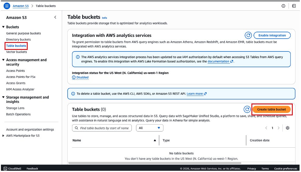
  1. On the left menu, select Table buckets.
  2. Choose the Create table bucket button.

Amazon S3 console showing the Table buckets management page in the US West (N. California) us-west-1 Region with zero table buckets, integration status disabled, and the Create table bucket button highlighted.

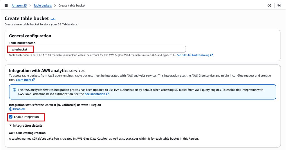
  1. In the next screen, we will fill the name of the bucket as salesbucket. Please ensure the Enable Integration configuration is checked. This step integrates S3 Tables with AWS Glue Data Catalog.

AWS S3 Create table bucket form with General configuration showing bucket name "salesbucket" and Integration with AWS analytics services section with Enable integration checkbox selected.

  1. Keep the other options as default and choose Create table bucket.
  2. After it is created, you will be redirected back to the list of table buckets. Choose the table bucket salesbucket.
  3. Select the Create table with Athena button.
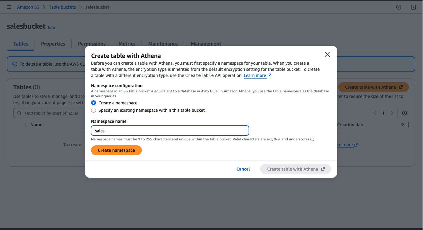
  4. Create a namespace in S3 Tables which is equivalent to a database in AWS Glue Data Catalog. Enter namespace (database) name as “sales” and click Create namespace.

Create table with Athena dialog in the Amazon S3 salesbucket console showing namespace configuration with "Create a namespace" selected and namespace name set to "sales."

  1. Choose Create table with Athena, and a new tab will be open with the Amazon Athena console.
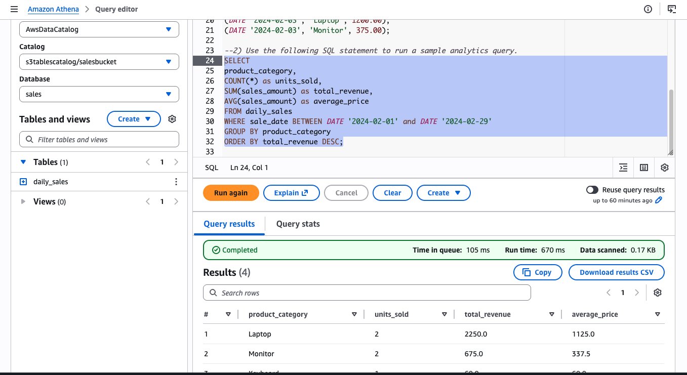
  2. When the Amazon Athena console opens, you will see an example of a query to create a table and examples to insert rows in that table. You could use this query block by uncommenting the code and executing each statement individually by highlighting it. At the end, you will have data in the table.

Amazon Athena query editor showing a SQL analytics query on the daily_sales table with results displaying product categories, units sold, total revenue, and average price for February 2024 sales data.

Query S3 Tables and create materialized view using Amazon EMR:

To run the instruction on Amazon EMR, complete the following steps to configure the cluster:

  1. Create an IAM role for the Amazon EMR instance profile following the Amazon EMR Management Guide. Add the following as policies and trust relationship for working on materialized views.

Replace ACCOUNT_ID with your AWS account ID, Instance_profile_role to the Amazon EMR instance profile role, and REGION with your AWS Region.

{
   "Version":"2012-10-17",
   "Statement":[
      {
         "Sid":"GlueDataCatalogPermissions",
         "Effect":"Allow",
         "Action":[
            "glue:GetCatalog",
            "glue:GetDatabase",
            "glue:CreateTable",
            "glue:GetTable",
            "glue:GetTables",
            "glue:UpdateTable",
            "glue:DeleteTable"
         ],
         "Resource":[
            "arn:aws:glue:<REGION>:<ACCOUNT ID>:catalog",
            "arn:aws:glue:<REGION>:<ACCOUNT ID>:catalog/s3tablescatalog",
            "arn:aws:glue:<REGION>:<ACCOUNT ID>:catalog/s3tablescatalog/*",
            "arn:aws:glue:<REGION>:<ACCOUNT ID>:database/salesdb",
            "arn:aws:glue:<REGION>:<ACCOUNT ID>:database/salesdb/*",
            "arn:aws:glue:<REGION>:<ACCOUNT ID>:database/s3tablescatalog",
            "arn:aws:glue:<REGION>:<ACCOUNT ID>:database/s3tablescatalog/*",
            "arn:aws:glue:<REGION>:<ACCOUNT ID>:table/s3tablescatalog/*",
            "arn:aws:glue:<REGION>:<ACCOUNT ID>:table/*/*"
         ]
      },
      {
         "Sid":"S3TablesDataAccessPermissions",
         "Effect":"Allow",
         "Action":[
            "s3tables:GetTableBucket",
            "s3tables:GetNamespace",
            "s3tables:GetTable",
            "s3tables:GetTableMetadataLocation",
            "s3tables:GetTableData",
            "s3tables:ListTableBuckets",
            "s3tables:CreateTable",
            "s3tables:PutTableData",
            "s3tables:UpdateTableMetadataLocation",
            "s3tables:ListNamespaces",
            "s3tables:ListTables",
            "s3tables:DeleteTable"
         ],
         "Resource":[
            "arn:aws:s3tables:<REGION>:<ACCOUNT ID>:bucket/*"
         ]
      },
      {
         "Effect":"Allow",
         "Action":"iam:PassRole",
         "Resource":"arn:aws:iam::<ACCOUNT ID>:role/service-role/<Instance_profile_role>"
      }
   ]
}

Add the following to the trust policy in addition to existing:

 {
            "Sid": "",
            "Effect": "Allow",
            "Principal": {
                "Service": "glue.amazonaws.com"
            },
            "Action": "sts:AssumeRole"
        }
  1. Launch an Amazon EMR cluster 7.12.0 or higher with instance profile role created in the previous step and with Iceberg enabled. For more information, refer to Use an Iceberg cluster with Spark.
  2. Connect to the primary node of your Amazon EMR cluster by using SSH, and run the following command to start a Spark application with the required configurations:

Replace bucket_name with your bucket name.

spark-sql \
  --conf spark.sql.extensions=org.apache.iceberg.spark.extensions.IcebergSparkSessionExtensions \
  --conf spark.sql.catalog.glue_catalog=org.apache.iceberg.spark.SparkCatalog \
  --conf spark.sql.catalog.glue_catalog.type=glue \
  --conf spark.sql.catalog.glue_catalog.warehouse=s3://<bucket_name> \
  --conf spark.sql.catalog.glue_catalog.glue.region=<region> \
  --conf spark.sql.catalog.glue_catalog.glue.id=<accountid>:s3tablescatalog/salesbucket \
  --conf spark.sql.catalog.glue_catalog.glue.account-id=<accountid> \
  --conf spark.sql.catalog.glue_catalog.client.region=<region> \
  --conf spark.sql.optimizer.answerQueriesWithMVs.enabled=true \
  --conf spark.sql.defaultCatalog=glue_catalog
  1. Run the following queries to query the daily_sales table.
spark-sql ()> use sales;
spark-sql (sales)> select * from daily_sales;
2024-01-15 Laptop 900.0
2024-01-15 Monitor 250.0
2024-01-16 Laptop 1350.0
2024-02-01 Monitor 300.0
2024-02-01 Keyboard 60.0
2024-02-02 Mouse 25.0
2024-02-02 Laptop 1050.0
2024-02-03 Laptop 1200.0
2024-02-03 Monitor 375.0
  1. Create Materialized view.
CREATE MATERIALIZED VIEW sales_mv as 
SELECT 
    product_category,
    COUNT(*) as units_sold,
    SUM(sales_amount) as total_revenue, 
    AVG(sales_amount) as average_price 
FROM 
    glue_catalog.sales.daily_sales 
GROUP BY 
    product_category;

A newly created materialized view is populated with the initial query results but does not update automatically as base table data changes. To keep it current, specify a REFRESH EVERY clause when creating the view. This accepts a time interval and unit, so you can define how often the materialized view is recomputed from the base tables.

  1. Add refresh interval.
CREATE MATERIALIZED VIEW sales_mv 
SCHEDULE REFRESH EVERY 2 HOURS as 
SELECT 
    product_category,
    COUNT(*) as units_sold,
    SUM(sales_amount) as total_revenue, 
    AVG(sales_amount) as average_price 
FROM 
    glue_catalog.sales.daily_sales 
GROUP BY 
    product_category;
  1. Alternatively, you can refresh them manually.

For manual full refresh, you can use the following command:

REFRESH MATERIALIZED VIEW sales_mv FULL;

For manual incremental refresh, you can use the following command:

REFRESH MATERIALIZED VIEW sales_mv;

For more details, refer to Refreshing materialized views.

  1. Query the MV.
spark-sql (sales)> select * from sales_mv
Keyboard 1 60.0 60.0
Laptop 4 4500.0 1125.0
Mouse 1 25.0 25.0
Monitor 3 925.0 308.3333333333333

After the Iceberg materialized views are created, you can access them using IAM principals that have required IAM permissions to Glue Data Catalog resource and its underlying storage.

Iceberg materialized views are flexible in how they combine base tables and access control modes. Base tables can reside in S3 general-purpose buckets (with IAM or Lake Formation access control), in S3 Tables (through the s3tablescatalog catalog), or a combination of these—all within a single materialized view definition. The materialized view itself can use either IAM or AWS Lake Formation access control, independently of its base tables.

For more details, refer to How materialized views work with AWS Glue.

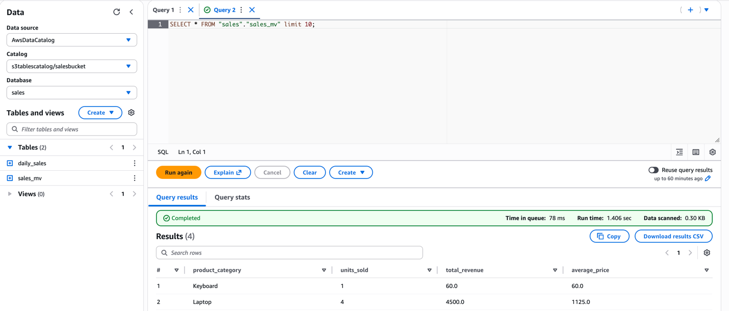
Query using Athena:

Additionally, you can query the same materialized view from Athena SQL. The following image shows the same query run on Athena and the resulting output.Amazon Athena query editor showing SELECT query results from the sales_mv materialized view with product category aggregations including Keyboard and Laptop sales data.

Query using Amazon Redshift:

To query the S3 Tables in AWS Glue Data Catalog using Amazon Redshift, you must create a database in the default catalog in Glue Data Catalog that points to the S3 Tables catalog.

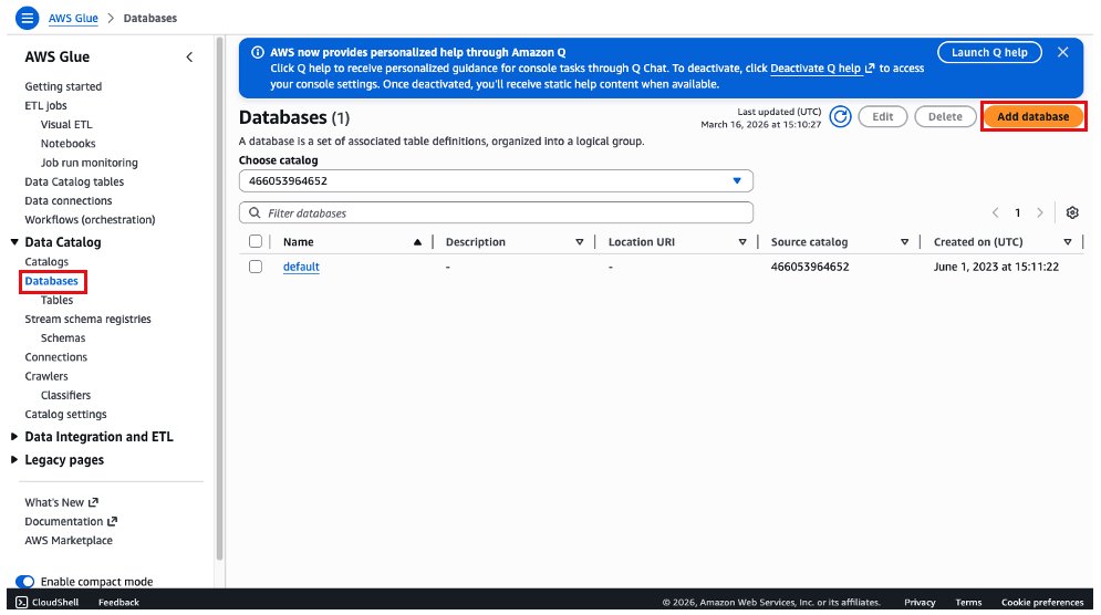
  1. On the AWS Glue console, choose Databases, and then choose Add Database.

AWS Glue Data Catalog Databases page showing one default database in catalog 466053964652, with the Add database button highlighted.

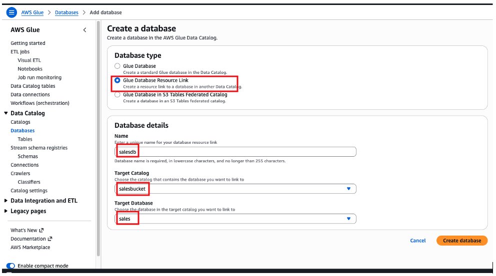
  1. Choose the Glue Database resource link option, add a name for the database, choose salesbucket on the target catalog and sales as the target database. Then select Create database.

AWS Glue Create a database form with Glue Database Resource Link selected, name set to "salesdb," target catalog "salesbucket," and target database "sales."

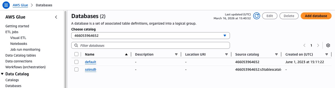
After creating the database, we will see the “salesdb” resource link under Databases on AWS Glue Data Catalog.

AWS Glue Data Catalog Databases page showing two databases: "default" and the newly created "salesdb" resource link with source catalog pointing to s3tablescatalog.

Create IAM role with the following policy for the Amazon Redshift schema creation. Replace the AWS Region and account ID for your account.

{
   "Version":"2012-10-17",
   "Statement":[
      {
         "Sid":"GlueDataCatalogPermissions",
         "Effect":"Allow",
         "Action":[
            "glue:GetCatalog",
            "glue:GetDatabase",
            "glue:CreateTable",
            "glue:GetTable",
            "glue:GetTables",
            "glue:UpdateTable",
            "glue:DeleteTable"
         ],
         "Resource":[
            "arn:aws:glue:<REGION>:<ACCOUNTID>:catalog",
            "arn:aws:glue:<REGION>:<ACCOUNTID>:catalog/s3tablescatalog",
            "arn:aws:glue:<REGION>:<ACCOUNTID>:catalog/s3tablescatalog/*",
            "arn:aws:glue:<REGION>:<ACCOUNTID>:database/salesdb",
            "arn:aws:glue:<REGION>:<ACCOUNTID>:database/salesdb/*",
            "arn:aws:glue:<REGION>:<ACCOUNTID>:database/s3tablescatalog",
            "arn:aws:glue:<REGION>:<ACCOUNTID>:database/s3tablescatalog/*",
            "arn:aws:glue:<REGION>:<ACCOUNTID>:table/s3tablescatalog/*",
            "arn:aws:glue:<REGION>:<ACCOUNTID>:table/*/*"
         ]
      },
      {
         "Sid":"S3TablesDataAccessPermissions",
         "Effect":"Allow",
         "Action":[
            "s3tables:GetTableBucket",
            "s3tables:GetNamespace",
            "s3tables:GetTable",
            "s3tables:GetTableMetadataLocation",
            "s3tables:GetTableData",
            "s3tables:ListTableBuckets",
            "s3tables:CreateTable",
            "s3tables:PutTableData",
            "s3tables:UpdateTableMetadataLocation",
            "s3tables:ListNamespaces",
            "s3tables:ListTables",
            "s3tables:DeleteTable"
         ],
         "Resource":[
            "arn:aws:s3tables:<REGION>:<ACCOUNTID>:bucket/*"
         ]
      }
   ]
}

Create an Amazon Redshift provisioned cluster or Amazon Redshift Serverless, attaching the IAM role created in previous step.

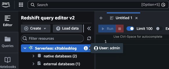
To access the AWS Glue Catalog and the resource link, you can now log in to Amazon Redshift as a local user. We use the admin user and Amazon Redshift Query Editor v2.

Amazon Redshift Query Editor v2 interface connected to Serverless workgroup "s3tablesblog" showing 2 native databases and 1 external database with an empty query editor ready for input.

To create the external schema, you must run the following command: Replace ACCOUNT_ID with your AWS Account ID, IAM_ROLE to IAM role created for schema access, and REGION with your AWS Region.

CREATE EXTERNAL SCHEMA salesdb
FROM DATA CATALOG DATABASE 'salesdb'
IAM_ROLE 'arn:aws:iam::<ACCOUNT_ID>:role/<IAM_ROLE>'
REGION '<REGION>'
CATALOG_ID '<ACCOUNT_ID>';

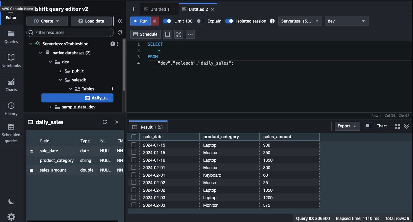
After you have created the external schema, it will show up on the left side, under the dev database. The table that we created, daily_sales, is available and we can query directly from Amazon Redshift using a local user.

Amazon Redshift Query Editor v2 showing a SELECT query on the daily_sales table in the salesdb schema with 9 rows of results displaying sale dates, product categories, and sales amounts from January–February 2024.

Cleanup:

After completing the walkthrough, follow these steps to remove the resources and avoid ongoing charges. These cleanup steps will permanently delete the data, including the daily_sales table and sales_mv materialized view. Make sure that you have backed up the data that you need to retain before proceeding.

To avoid incurring future charges, clean up the resources that you created during this walkthrough:

  • Remove the Glue Data Catalog resources
  • Delete the table bucket
  • Terminate and Delete the Amazon Redshift cluster
  • Terminate and Delete the Amazon EMR cluster
  • Delete the IAM roles/policies created

Conclusion

Amazon S3 Tables now integrate with AWS Glue Data Catalog through IAM-based authorization via a single IAM policy. By consolidating permissions for storage, catalog, and query engines into one IAM policy, you can streamline authorization with AWS analytics services like Amazon Athena, Amazon EMR, and AWS Glue. You can use this streamlined IAM authorization model to build your data lake faster while maintaining enterprise-grade security. For organizations with additionally granular data access requirements, AWS Lake Formation remains available to layer fine-grained access controls on top of this foundation. This is configurable through the AWS Management Console, CLI, API, or CloudFormation. This integration allows AWS analytics users to use IAM and scale their analytics capabilities with reduced operational complexity.

To learn more about to S3 Tables and integration with Glue Data catalog, visit: Amazon S3 Tables integration with AWS analytics services overview and Integrating with Amazon S3 Tables.


About the authors

Ricardo Serafim

Ricardo is a Senior Analytics Specialist Solutions Architect at AWS. He has been helping companies with Data Warehouse solutions since 2007.

Milind Oke

Milind is a Data Warehouse Specialist Solutions Architect based out of New York. He has been building data warehouse solutions for over 15 years and specializes in Amazon Redshift.

Pratik Das

Pratik is a Senior Product Manager with AWS Lake Formation. He is passionate about all things data and works with customers to understand their requirements and build delightful experiences. He has a background in building data-driven solutions and machine learning systems.

Srividya Parthasarathy

Srividya is a Senior Big Data Architect on the AWS Lake Formation team. She works with the product team and customers to build robust features and solutions for their analytical data platform. She enjoys building data mesh solutions and sharing them with the community.

Choosing between single or multiple organizations in AWS Organizations

Post Syndicated from John White original https://aws.amazon.com/blogs/architecture/choosing-between-single-or-multiple-organizations-in-aws-organizations/

Organizations face critical architectural decisions that can impact their operations for years to come. Recently, I had the opportunity to collaborate with a cloud migration advisor on a question that challenges many enterprises during their cloud adoption journey: Is it better to maintain a single organization or implement multiple organizations? This same question was also asked on re:Post.

This question isn’t merely academic—it strikes at the heart of how businesses balance governance, security, cost efficiency, and operational flexibility in their cloud environments. With many partners and customers growing through acquisitions, reorganizations, or organic expansion, understanding the implications of AWS Organizations becomes increasingly important.

The discussion yielded a comprehensive analysis of key criteria that decision-makers should consider when evaluating their cloud organization strategy. Although maintaining separate organizations might offer stronger isolation and customized governance in the short term, the long-term benefits of consolidation—including volume discounts, simplified resource sharing, and reduced operational overhead—often make a compelling case for eventual migration to a single organization.

In this post, I explain the key advantages and disadvantages of both approaches and the scenarios where each model fits best.

AWS Organizations: The foundation for multi-account strategy

AWS Organizations provides a centralized way to manage multiple AWS accounts. With AWS Organizations, you can:

  • Consolidate billing across accounts.
  • Apply policies centrally using service control policies (SCPs).
  • Share resources between accounts such as virtual private clouds (VPCs) and directory services.
  • Enforce consistent governance through organizational units (OUs).

How it works

Most AWS customers adopt a single organization and create multiple accounts within it. However, some enterprises—particularly those with highly independent business units or strong regulatory requirements or those experiencing mergers and acquisitions—explore the option of creating multiple organizations.

With AWS Organizations, you can manage your accounts through the following steps:

  • Add accounts. Create new accounts or invite existing accounts to your organization.
  • Group accounts. Group accounts into organizational units (OUs) by use-case or workstream.
  • Apply policies. Apply policies to accounts or OUs, such as service control policies (SCPs) which create permission boundaries.
  • Enable AWS services. Enable AWS services integrated with AWS Organizations.

When to use a single organization

For most customers, a single organization provides the right balance of control, cost efficiency, and governance. This approach works well when:

  • You want centralized visibility and governance across AWS accounts.
  • Teams and business units operate under a shared corporate security policy.
  • You want to consolidate billing and optimize for volume discounts.
  • You want to share resources (such as networking or directory services) between accounts.
  • You want centralized compliance enforcement using SCPs, AWS Config, and AWS Security Hub.

A use case in which a single organization is preferred is a large global retailer with regional teams and application owners. Each team creates their own AWS accounts under a central IT governance framework. A core team is responsible for centrally managing regulatory and security standards across the entire company.

When to consider multiple organizations

There are cases where creating multiple organizations might make sense. These typically arise when:

  • You have independent business units with separate leadership, governance, and security requirements (for example, subsidiaries or franchises).
  • You’re in a regulated industry where strict segmentation between entities is legally required (for example, banking or healthcare).
  • You’re managing mergers and acquisitions, where newly acquired companies maintain their existing AWS footprint.
  • You want maximum isolation of the potential impact of issues, so that misconfigurations, security incidents, or policy changes in one organization don’t affect others.

An example of a situation where multiple organizations is preferred is a multinational financial services company with distinct retail banking, investment banking, and insurance divisions. Each division has its own regulatory body and distinct security requirements, so they each manage their own organization.

Another example might be a global software company that uses a separate organization as a sandbox to develop and test guardrails and SCPs prior to applying them to their primary organization.

Operational efficiency compared to risk isolation

When deciding between using single or multiple organizations, enterprises must balance operational efficiency with risk isolation. A single organization provides simplified management, volume discounts, and easier resource sharing and governance. Structuring the enterprise with multiple organizations means stronger security and failure isolation, greater governance flexibility, and better support for organizational autonomy.

The following table summarizes the core differences between these two approaches.

Criteria Single organization Multiple organizations
Billing Consolidated billing with volume discounts across accounts Each organization has independent billing; no cross- organization discounts
Governance Centralized SCPs and policies for accounts Each organization defines its own governance policies
Security isolation Shared security perimeter; SCPs apply globally Strong isolation between organizations
Access management Central AWS Identity and Access Management (IAM) roles and cross-account access setup No built-in cross- organization access; fully independent IAM
Scalability Supports thousands of accounts within a single organization Each organization is independent; you scale organizations separately
Resource sharing Easy sharing of VPCs, Amazon Machine Images (AMIs), and other resources within organization No built-in sharing between organizations
Operational overhead Lower; centralized governance reduces duplication Higher; governance, security, and operations duplicated per organization
Compliance and audit Centralized logging, AWS CloudTrail, and AWS Config across accounts Requires separate audit trails per organization
Risk isolation Misconfigurations could impact accounts Misconfigurations are contained within individual organizations
Flexibility Standardized controls across accounts Each organization can tailor controls to its specific needs

Conclusion

Most enterprises, especially those adopting AWS as part of a centralized IT strategy, find that a single organization is the best fit. However, for conglomerates, regulated businesses, and companies growing through acquisition, multiple organizations might be appropriate.

When helping customers design their AWS multi-account strategy, I recommend starting with a single organization and only considering multiple organizations when the isolation requirements outweigh the operational benefits of centralization.

For more information, refer to the following resources:


About the Authors

Improve DynamoDB analytics with AWS Glue zero-ETL schema and partition controls

Post Syndicated from Raju Ansari original https://aws.amazon.com/blogs/big-data/improve-dynamodb-analytics-with-aws-glue-zero-etl-schema-and-partition-controls/

You store transactional data in Amazon DynamoDB and get single-digit millisecond performance. However, when you want to run analytics, machine learning (ML), or reporting on that same data, you face a gap: your flexible, semi-structured DynamoDB schemas don’t align with the flat, columnar formats that analytics engines require. Bridging this gap typically means building and maintaining custom ETL pipelines, which adds development cost and operational overhead.

AWS Glue Zero-ETL integration removes that pipeline work. It enables replication of your DynamoDB tables to Apache Iceberg tables in Amazon Simple Storage Service (Amazon S3), then query it directly with Amazon Athena. During setup, you can configure two capabilities that will shape how replicated data looks and performs: schema unnesting flattens nested attributes into individual columns, and data partitioning organizes data so your queries scan only what they need.

In this post, you learn how to replicate Amazon DynamoDB data to Apache Iceberg tables in Amazon S3 through a zero-ETL integration. We walk through the challenges that the DynamoDB nested, schema-flexible data model introduces for analytics workloads, and show you how to configure schema unnesting and data partitioning for a sample product catalog table. We also cover how to query the replicated data in Amazon Athena using standard SQL.

Semi-structured data meets analytics

Your product catalog in DynamoDB contains items with nested attributes like product details, pricing tiers, and inventory information. A typical item looks like this:

{
  "product_id": "P-1001",
  "name": "Wireless Headphones",
  "productdetails": {
    "brand": "AudioTech",
    "category": "Electronics",
    "weight_kg": 0.25,
    "specification": {
       "color": "Black",
       "storage": "128GB"
    }
  },
  "pricing": {
    "list_price": 79.99,
    "discount_pct": 10
  },
  "created_at": 1701388800000
}

This structure supports fast transactional reads and writes. However, when you replicate this data for analytics, you face two decisions:

  • You must decide whether to flatten nested maps like productdetails into individual columns or preserve them as-is.
  • You must choose how to organize the data on disk so that queries filtering by brand or date range scan only relevant partitions.

With AWS Glue Zero-ETL, you address both decisions through configurable schema unnesting and data partitioning.

Solution overview

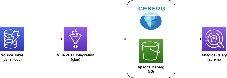
You replicate data from your DynamoDB table through AWS Glue Zero-ETL into Apache Iceberg tables stored in Amazon S3, then query the results with Amazon Athena. The following diagram illustrates the end-to-end architecture:

Data flow diagram showing AWS data pipeline: DynamoDB source table → AWS Glue zero-ETL integration → Apache Iceberg on Amazon S3 → Amazon Athena analytics query.

AWS Glue zero-ETL ingests data from Amazon DynamoDB, writes it in Apache Iceberg format to your Amazon S3 data lake, and makes it available for SQL queries in Amazon Athena—with no pipelines to build or maintain. With this integration, you:

  • Save development time by skipping custom code and ETL job management
  • Keep DynamoDB performance intact because replication doesn’t consume table’s provisioned read/write capacity
  • Get data within 15 minutes of changes in the source table
  • Query with standard tools because data lands in Apache Iceberg format, an open table format that AWS natively supports for high-performance analytics

During setup, you configure two output settings:

  1. Schema unnesting in Zero-ETL: You choose how nested attributes appear in the target. Flattening nested maps into individual columns streamlines your queries and reduces complexity.
  2. Data partitioning in Zero-ETL: You choose how data is organized into partitions. When you filter on a partition column, the query engine reads only matching data instead of scanning everything, cutting both query time and cost.

Schema unnesting

When you create a zero-ETL integration, you can choose one of three unnesting options. Schema unnesting transforms complex, nested DynamoDB structures into formats that analytics engines can query directly, removing post-processing transformations.

Each option changes how nested DynamoDB attributes appear in the target table. The right choice depends on your analytics tools and how consistent your DynamoDB schemas are.

Option 1: No unnesting

This option preserves the original nested structure. DynamoDB maps and lists remain as structured columns in the target.

Using the product example, the target table retains productid and value as columns to hold DynamoDB partition key and a DynamoDB record respectively.

Recommended for: Workloads where your analytics tools natively support querying nested data and you want to preserve the DynamoDB structure unchanged.

Option 2: Unnest one level

This option flattens top-level maps into individual columns. Lists remain nested.

With this option, productdetails and pricing each become separate columns.

Recommended for: Scenarios where your DynamoDB items have a consistent schema and you want to balance structure preservation with query simplicity.

Option 3: Unnest all levels (default)

This option recursively flattens nested structures using dot notation and produces the flattest schema.

For the product table, this creates columns such as productdetails.brand, productdetails.category, productdetails.specification.color , productdetails.specification.storage , pricing.list_price, and pricing.discount_pct. The pricing map flattens similarly. Each column is directly queryable without nested access patterns.

Recommended for: Analytics tools that prefer flat schemas when your DynamoDB items have a reasonably consistent structure. Note that deeply nested or highly variable schemas can produce very wide tables.

Data partitioning

You can speed up your queries and reduce costs by partitioning your replicated data. Partitioning divides data into logical segments on disk.

When you include a filter on a partition column in your query, the query engine skips irrelevant segments entirely. This behavior is called partition pruning: instead of scanning the entire dataset, the engine reads only the data that matches your filter conditions. For large tables, partition pruning can reduce both query runtime and cost significantly.

Default partitioning

If you don’t specify partition columns, AWS Glue Zero-ETL partitions data using the DynamoDB primary key with bucketing. This approach supports general-purpose queries without requiring manual configuration. For specific query patterns or performance requirements, you can define custom partitioning strategies described in the subsections that follow.

Identity partitioning

Identity partitioning uses raw column values to create partitions. You apply this strategy to low-to-medium cardinality columns such as brand, category, or AWS Region. To partition the product table by productdetails.brand and create a separate partition for each brand, use this configuration:

{
  "partitionSpec": [
    {
      "fieldName": "productdetails.brand",
      "functionSpec": "identity"
    }
  ]
}

With this setup, AWS Glue creates one partition directory per unique brand value. When you query for a specific brand, Athena reads only that partition.

Important: Avoid identity partitioning on high-cardinality columns such as primary keys or timestamps. This creates many small partitions, which degrades both ingestion and query performance

Time-based partitioning

Time-based partitioning organizes data by timestamp at a chosen granularity: year, month, day, or hour. You apply this strategy to time-series data and time-range queries. To partition the product table by month on the created_at column, which stores epoch milliseconds, use this configuration:

{
  "partitionSpec": [
    {
      "fieldName": "created_at",
      "functionSpec": "month",
      "conversionSpec": "epoch_milli"
    }
  ]
}

The conversionSpec parameter tells AWS Glue how to interpret the source timestamp. Supported values: epoch_sec (Unix seconds), epoch_milli (Unix milliseconds), and iso (ISO 8601 format).

Note: The original column values remain unchanged. AWS Glue transforms only the partition column values to timestamp type in the target table

Multi-level partitioning

You can combine strategies for a hierarchical scheme. To partition first by month and then by brand, use this configuration:

{
  "partitionSpec": [
    {
      "fieldName": "created_at",
      "functionSpec": "month",
      "conversionSpec": "epoch_milli"
    },
    {
      "fieldName": "productdetails.brand",
      "functionSpec": "identity"
    }
  ]
}

This scheme supports efficient queries that filter by date range, brand, or both. Place higher-selectivity columns first in the hierarchy and align the scheme with your most common query patterns.

Best practices

Keep these guidelines in mind when you configure your integration:

  • Avoid identity partitioning on high-cardinality columns such as primary keys, timestamps, or system-generated IDs. This leads to partition explosion and degrades performance.
  • Apply only one time-based function per column. For example, don’t partition col1 by year, month, day, and hour simultaneously.
  • Match conversionSpec to your actual data format. If your timestamps are in epoch milliseconds, use epoch_milli, not epoch_sec or iso.
  • Choose granularity based on data volume. High-volume tables benefit from finer granularity (day or hour). Lower-volume tables work well with coarser granularity (month or year).
  • Account for timezone implications with ISO timestamps. AWS Glue Zero-ETL normalizes timestamp partition values to UTC.

Prerequisites

To implement the AWS Glue Zero-ETL integration with a DynamoDB source, you will need:

  1. An AWS account with least privilege principle
  2. An AWS Glue database (for example, ddb_zero_etl_demo_db) with an Amazon S3 bucket associated as the database location (setup instructions)
  3. AWS Glue Data Catalog settings updated with an AWS Identity and Access Management (IAM) policy that grants fine-grained access control for zero-ETL (setup instructions)
  4. Create an IAM role named zetl-role, to be used by zero-ETL to access data from your DynamoDB table
  5. A DynamoDB source table (for example, product) configured for zero-ETL integration (setup instructions)

Walkthrough: Create the zero-ETL integration

Complete these steps to create a zero-ETL integration with DynamoDB as the source and Apache Iceberg tables in Amazon S3 as the target.

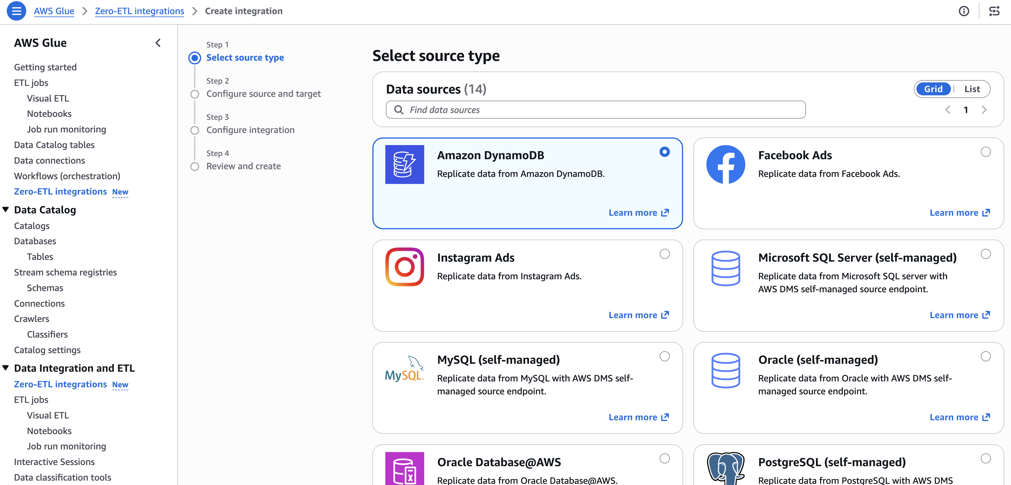
Step 1: Select the source type

  1. Open the AWS Glue console.
  2. In the navigation pane, under Data Integration and ETL, choose Zero-ETL integrations.
  3. Choose Create zero-ETL integration.
  4. Select Amazon DynamoDB as the source type, then choose Next.

AWS Glue console showing Step 1 of creating a Zero-ETL integration — selecting a source type from 14 available data sources including Amazon DynamoDB, Facebook Ads, Instagram Ads, MySQL, Oracle, PostgreSQL, and Microsoft SQL Server

[Figure 1: Selecting Amazon DynamoDB as the zero-ETL source type]

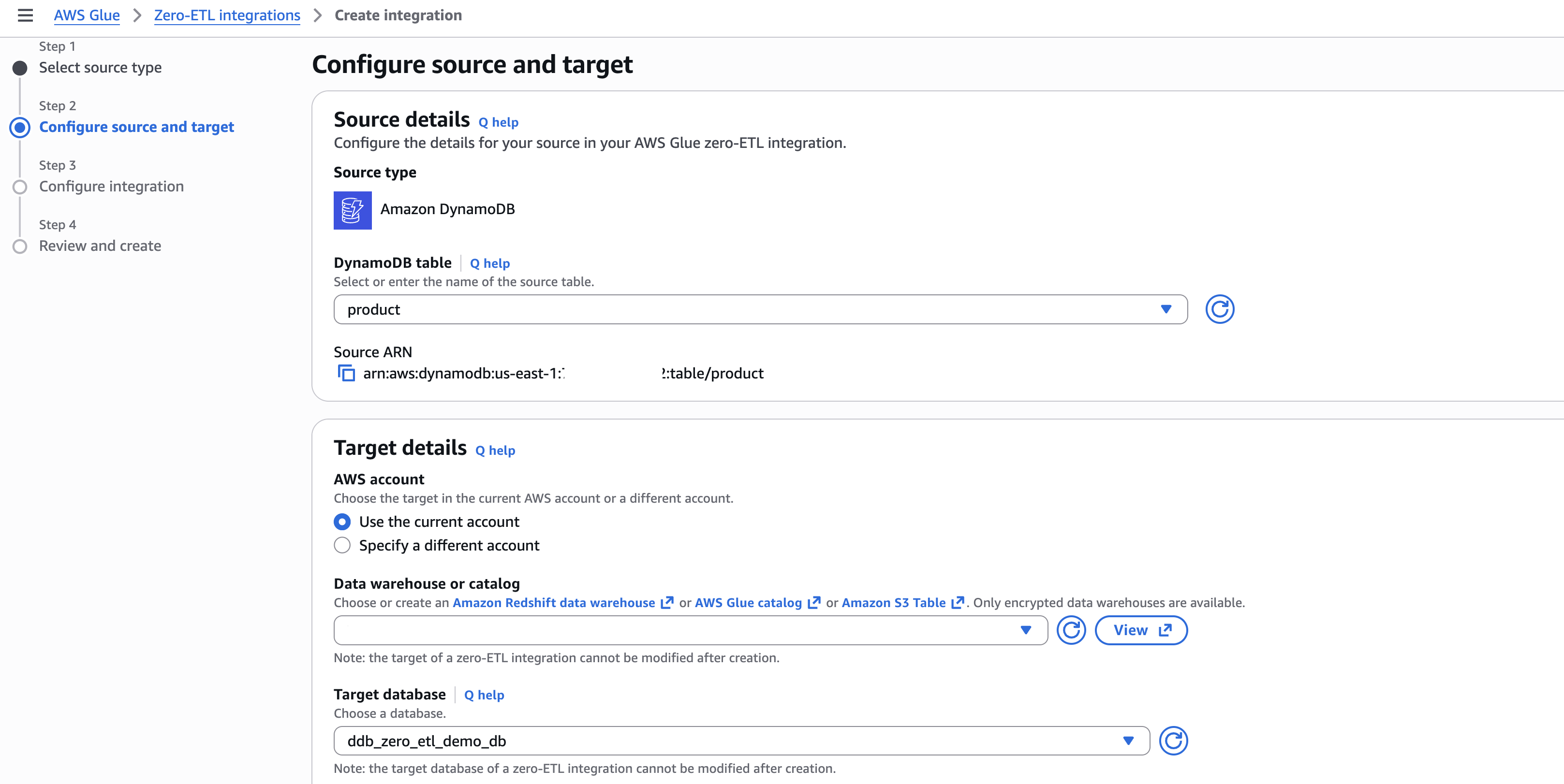
Step 2: Configure source and target

  1. In Source details, select your DynamoDB table (for example, product).
  2. In Target details:
    • Select the current account as target.
    • Choose the catalog and target database (for example, ddb_zero_etl_demo_db).
    • Select the IAM role (for example, zetl-role).

AWS Glue console Step 2 — configuring source and target for a zero-ETL integration with Amazon DynamoDB "product" table as source and an AWS Glue catalog database "ddb_zero_etl_demo_db" as target

[Figure 2: Configuring source DynamoDB table and target database]

Step 3: Configure output settings

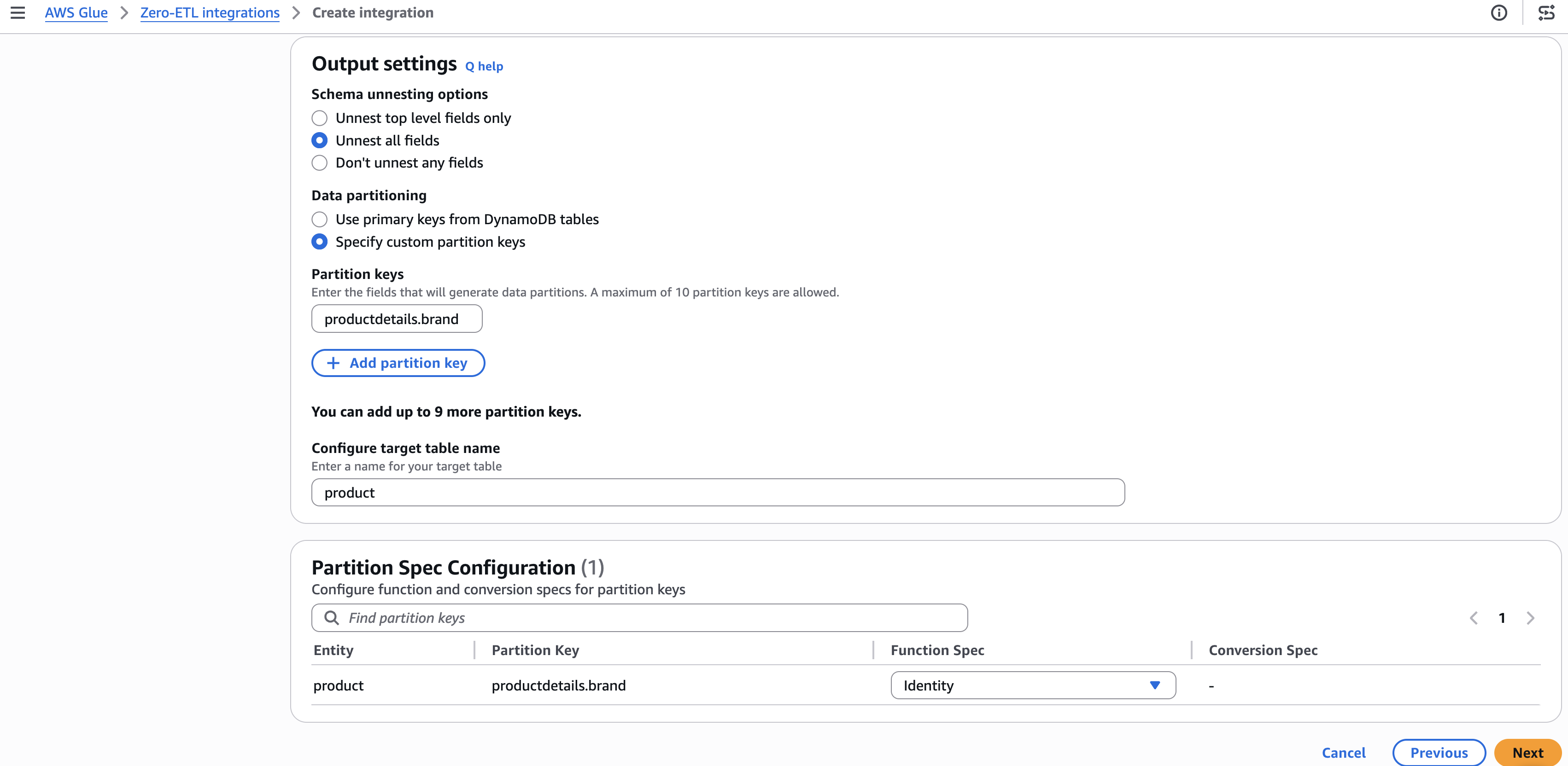
  1. Under Schema unnesting, select Unnest all fields.
  2. Under Data partitioning, select Specify custom partition keys.
  3. Enter the partition key (for example, productdetails.brand) and set the function to Identity.
  4. Choose Next.

AWS Glue Zero-ETL integration output settings showing schema unnesting set to "Unnest all fields," custom partition key "productdetails.brand" configured with Identity function, and target table named "product.

[Figure 3: Configuring schema unnesting and partition key settings]

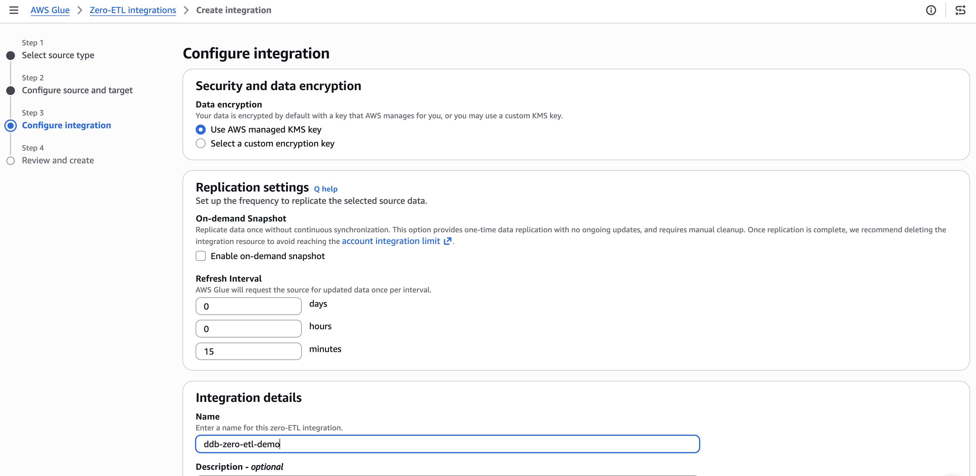
Step 4: Set integration details

  1. Optionally configure encryption and replication settings. The default refresh interval is 15 minutes.
  2. Enter a name for the integration (for example, ddb-zero-etl-demo).
  3. Choose Next.

AWS Glue Zero-ETL integration Step 3 — configuring security with AWS managed KMS key, replication refresh interval set to 15 minutes, and integration named "ddb-zero-etl-demd

[Figure 4: Configuring encryption and replication settings]

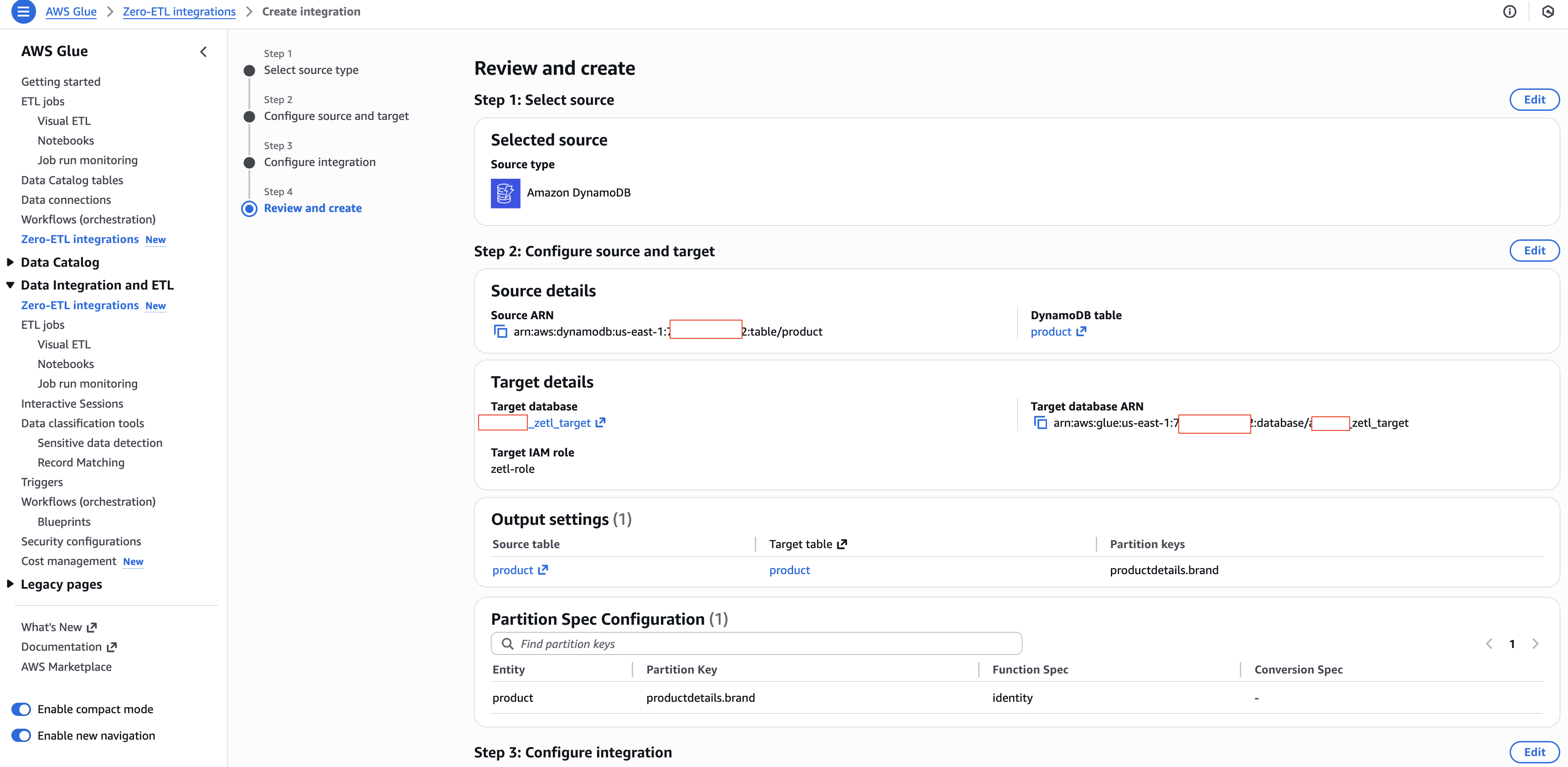
Step 5: Review and create

  1. Review your settings and choose Create and launch integration.
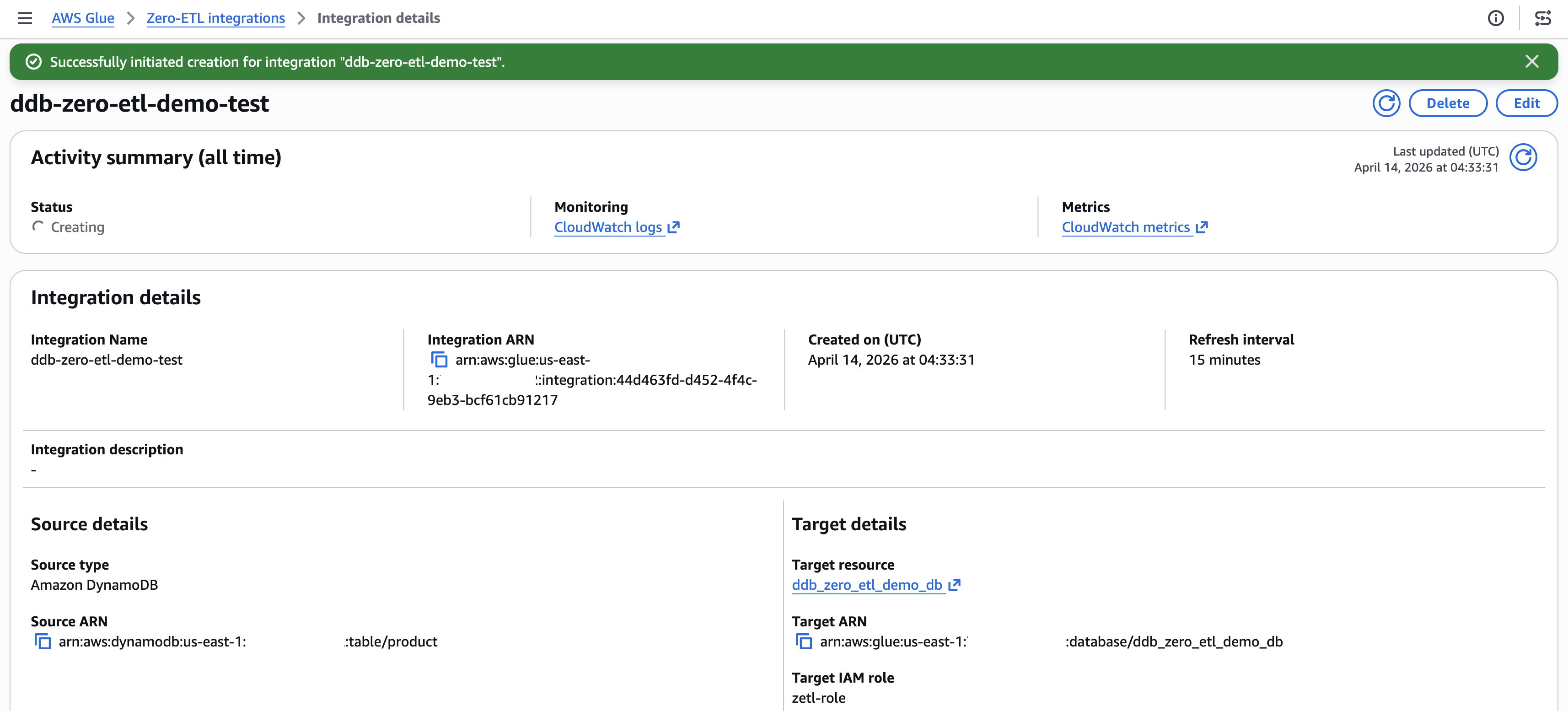
  2. The integration shows as Active within about a minute.

AWS Glue Zero-ETL integration Step 4: Review and Create — showing DynamoDB "product" table as source, Glue database "zett_target" as target with IAM role "zett-role," and partition key "productdetails.brand" with Identity function

[Figure 5: Review and create summary]

AWS Glue Zero-ETL Integration Details page showing "ddb-zero-etl-demo-test" integration with status "Creating," DynamoDB "product" table as source, Glue database "ddb_zero_etl_demo_db" as target, and a 15-minute refresh interval

[Figure 6: Integration active with successful status]

Query the replicated data

After the integration is active and the initial replication completes (typically 15–30 minutes), you can query the data in Amazon Athena.

Preview the replicated data

  1. Open the Amazon Athena console.
  2. In the query editor, select your target database (for example, ddb_zero_etl_demo_db).
  3. Run a preview query:
SELECT * FROM "ddb_zero_etl_demo_db"."product"LIMIT 10;

Verify schema unnesting

With Unnest all fields selected, nested attributes appear as individual columns with dot notation:

SELECT "productdetails.brand", "productdetails.category", "pricing.list_price" 
FROM "ddb_zero_etl_demo_db"."product"
WHERE "productdetails.category" = 'Electronics';

Verify partition pruning

Queries that filter on the partition column (productdetails.brand) automatically skip irrelevant partitions:

SELECT product_id, name, "pricing.list_price"
FROM "ddb_zero_etl_demo_db"."product"
WHERE "productdetails.brand" = 'AudioTech';

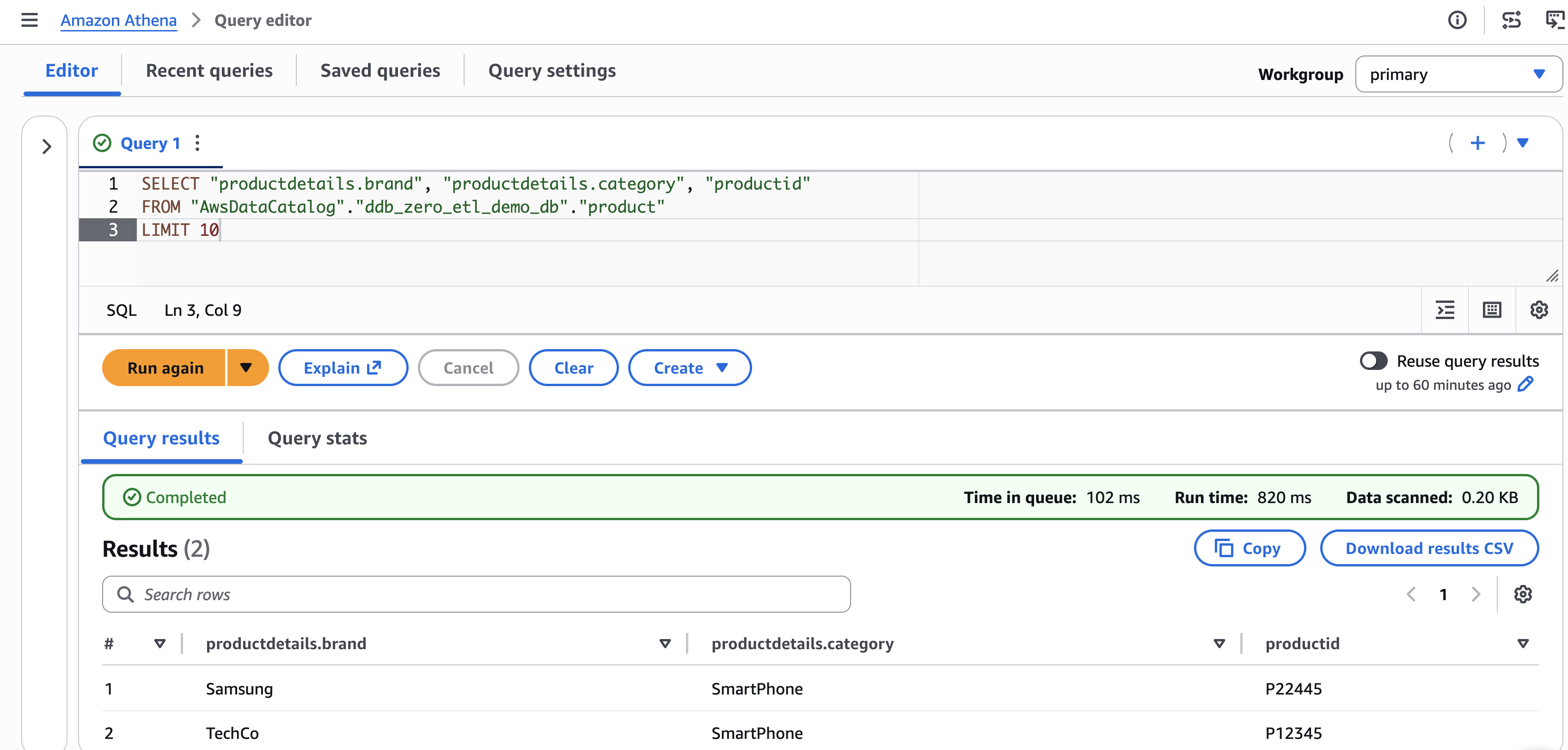
Amazon Athena Query Editor showing a completed SQL query selecting brand, category, and product ID from a DynamoDB zero-ETL Glue catalog table, returning two results: Samsung SmartPhone P22445 and TechCo SmartPhone P12345

[Figure 7: Athena query to retrieve the data from Apache Iceberg lakehouse]

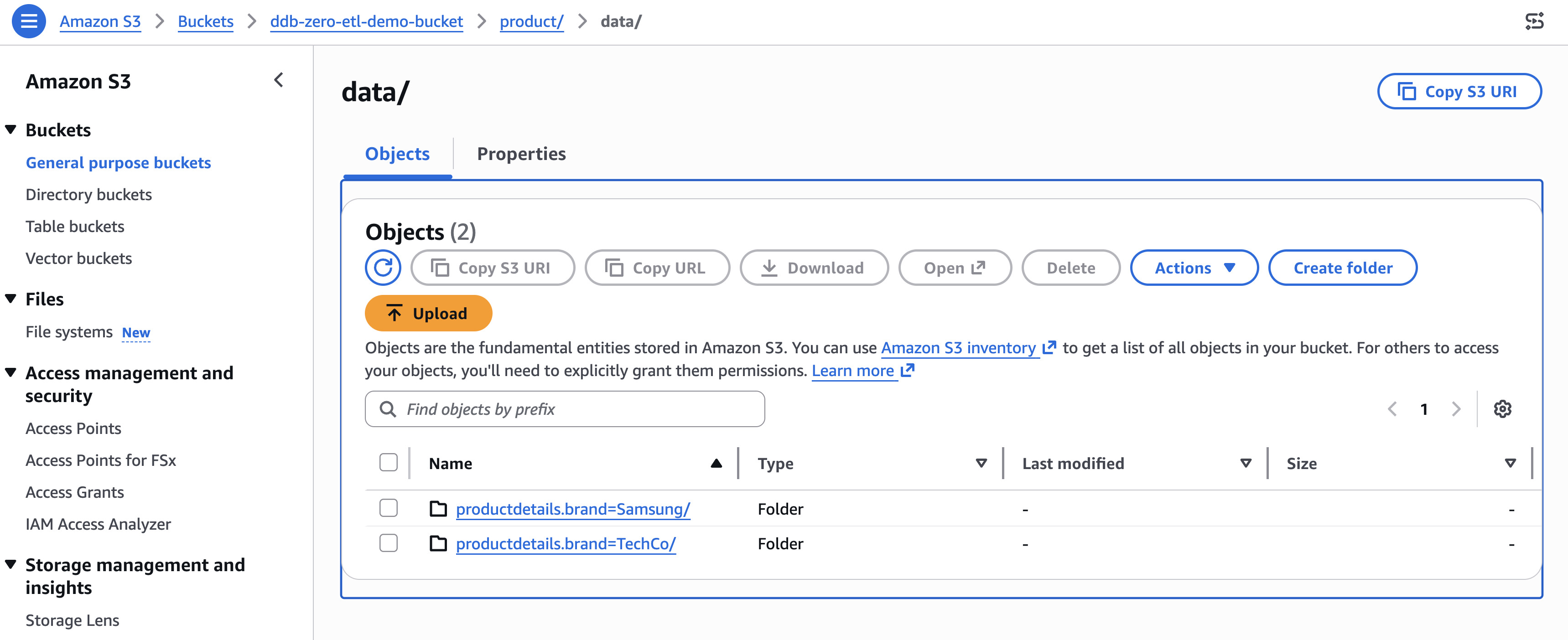
You can verify the partition structure by navigating to the Amazon S3 bucket associated with your database. The data organizes into directories like:

Amazon S3 bucket browser showing the "data/" folder in "ddb-zero-etl-demo-bucket" with two partitioned folders: "productdetails.brand=Samsung/" and "productdetails.brand=TechCo/" — confirming Iceberg partition structure from DynamoDB zero-ETL integration

[Figure 8: Amazon S3 bucket organization for the identity partition productdetails.brand]

Clean up

To avoid ongoing charges, delete the resources in this order:

  1. Delete the zero-ETL integration. In the AWS Glue console, navigate to Zero-ETL integrations, select your integration, and choose Delete. Existing replicated data remains in the target, but new changes stop replicating.
  2. Delete the replicated table. In the AWS Glue Data Catalog, navigate to Tables, select the replicated table, and delete it.
  3. Delete the AWS Glue database. In the Data Catalog, select the database and delete it.
  4. Delete the Amazon S3 data. Empty and delete the S3 bucket associated with the database.
  5. Delete the DynamoDB table. If you created it for this walkthrough, delete the source table.
  6. Delete IAM resources. Remove the IAM role and policies created for the integration.

Conclusion

You configured schema unnesting and data partitioning for a DynamoDB zero-ETL integration, replicated a product catalog table to Apache Iceberg tables in Amazon S3, and verified the results in Amazon Athena. Unnesting flattened nested attributes into directly queryable columns. Partitioning helped the query engine skip irrelevant data, reducing both query time and cost. To take your integration further, try monitoring replication lag and data freshness with Amazon CloudWatch metrics. You can also experiment with different partitioning strategies on a staging table before applying them to production workloads, testing time-based partitioning alongside identity partitioning to find the optimal scheme for your query patterns. For broader analytics coverage, query the same Iceberg tables from Amazon Redshift Spectrum or Amazon EMR alongside Athena. For more details, explore these resources:


About the authors

Raju Ansari

Raju is a Senior Software Development Engineer at AWS, specializing in building scalable, secure, serverless solutions that simplify data analytics and AI agent development. He helps organizations modernize their data analytics infrastructure and develop cutting-edge AI agentic applications. Currently, Raju focuses on building foundational AI services, including Amazon Bedrock Agents, which enable developers to create intelligent, autonomous applications at scale. Outside of work, Raju is passionate about giving back to the tech community. He actively volunteers at IEEE events and mentor early and mid-career professionals

Shashank Sharma

Shashank is an Engineering Leader with over 15 years of experience delivering data integration and replication solutions for first-party and third-party databases and SaaS for enterprise customers. He leads engineering for AWS Glue Zero-ETL and Amazon AppFlow, building fully managed pipelines that replicate data from sources like Salesforce, SAP, DynamoDB, and Oracle into Amazon Redshift and Apache Iceberg-based data lakes. Shashank advises startups on technology strategy and mentors engineers and technical leaders at various career stages

How to build a cross-Region resilience for Amazon OpenSearch Service with Amazon MSK

Post Syndicated from Sriharsha Subramanya Begolli original https://aws.amazon.com/blogs/big-data/how-to-build-a-cross-region-resilience-for-amazon-opensearch-service-with-amazon-msk/

Cross-Region resilience for Amazon OpenSearch Service has historically been a complex challenge, relying on S3-based snapshots or cross-cluster replication that demand intricate manual failover procedures often resulting in hours of downtime, data inconsistencies, and significant lag during outages, or other operational disruptions. To overcome these limitations and help businesses stay focused on their core objectives, we’ve developed a solution that automatically maintains synchronized data across AWS Regions while supporting active-active operations in both AWS Regions.

AWS offers two OpenSearch offerings, namely Amazon OpenSearch Service, a managed cluster-based service where you provision and manage OpenSearch domains (nodes, storage, scaling), and Amazon OpenSearch Serverless, a serverless option where AWS automatically manages infrastructure and scaling and you create collections for your search or analytics workloads. OpenSearch Service provides high availability (HA) within an AWS Region through its Multi-AZ deployment model and provides Regional resiliency with cross-cluster replication. Amazon Managed Streaming for Apache Kafka (Amazon MSK) Replicator is an Amazon MSK feature that you can use to reliably replicate data across Amazon MSK clusters in different or the same AWS Region.

In this post, we outline the solution that provides cross-Region resiliency without needing to reestablish relationships during a fail-back, using an active-active replication model with Amazon OpenSearch Ingestion (OSI) and Amazon Managed Streaming for Apache Kafka (Amazon MSK). This solution applies to both OpenSearch Service managed clusters and Amazon OpenSearch Serverless collections. We use Amazon OpenSearch Serverless as an example for the configurations in this post.

Solution overview

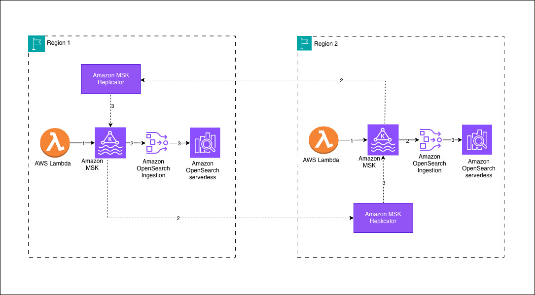
In this solution we use Amazon MSK Replicator for bidirectional cross-Region data replication, with OSI pipelines to index data into Amazon OpenSearch Serverless collections in each AWS Region. While the S3 based approach serves the purpose, Amazon MSK Replicator provides near real-time replication with identical topic naming, which supports active-active operations. Amazon MSK Replicator provides automatic loop prevention and consumer group offset synchronization, enabling seamless cross-Region failover. You can find the code for the entire solution in the GitHub repo.

Your architecture will follow a Regional-first approach where data sources write to a local Amazon MSK cluster within their AWS Region. In this sample deployment, an AWS Lambda function serves as the producer, streaming data into the MSK cluster. OSI pipelines consume the incoming data from the local MSK cluster and persist it to an Amazon OpenSearch Serverless collection within the same AWS Region. To achieve cross-Region data synchronization, Amazon MSK Replicator facilitates bidirectional replication between the Amazon MSK clusters, preserving the same topic names across both environments. This design validates that Amazon OpenSearch Serverless collections in each AWS Region maintain identical datasets, provides low-latency search capabilities and high availability for globally distributed workloads.
Prerequisites

Deploy the AWS Cloudformation template to install the prerequisites. The solution has the following prerequisite steps:

  1. Set up Amazon Virtual Private Cloud (Amazon VPC) infrastructure in both Regions
    1. Create Amazon VPCs with private subnets in at least two or three Availability Zones for high availability at the AWS Region level
    2. Configure Network Address Translation (NAT) Gateways for outbound internet access from private subnets
    3. Use non-overlapping CIDR blocks
  2. Establish Amazon OpenSearch Serverless collections in both AWS Regions
  3. Create Amazon OpenSearch Serverless Collections for log analytics
  4. Configure encryption, network, and data access policies
  5. Create Amazon VPC endpoints for private access
  6. Configure MSK clusters in both AWS Regions
  7. Enable AWS Identity and Access Management (IAM) authentication (SASL/IAM)
  8. Enable Multi-VPC connectivity (required for Amazon MSK Replicator and OSI)
  9. Configure MSK cluster policies to allow kafka.amazonaws.com and osis-pipelines.amazonaws.com service principals
  10. Configure IAM permissions for pipeline and replication access
  11. Create IAM roles for the OSI pipelines with permissions to access Amazon Managed Streaming for Apache Kafka and Amazon OpenSearch Serverless.
  12. Create IAM roles for the Amazon MSK Replicator with permissions for cross-Region access to Amazon Managed Streaming for Apache Kafka clusters.

This AWS CloudFormation template helps you in deploying all of the required configurations with primary AWS Region as us-east-1 and secondary AWS Region as us-west-2.

The following snippets shows the configuration for the OSI pipeline, which writes data from Amazon MSK to Amazon OpenSearch Serverless. The OSI pipeline uses MSK as a source with IAM authentication.

version: "2"
kafka-pipeline:
source:
kafka:
acknowledgments: true
topics:
- name: "opensearch-data"
group_id: "osi-consumer-group-primary"
aws:
msk:
arn: "arn:aws:kafka:us-east-1:<aws-acccount-id>:cluster/production-msk-primary/CLUSTER_ID"
region: "us-east-1"
sts_role_arn: "arn:aws:iam::<aws-acccount-id>:role/production-osi-pipeline-primary-role"
sink:
- opensearch:
hosts:
- "https://<OPENSEARCH_SERVERLESS_COLLECTION_ID>.us-east-1.aoss.amazonaws.com"
index: "application-logs-${yyyy.MM.dd}"
aws:
serverless: true
region: "us-east-1"
sts_role_arn: "arn:aws:iam::<aws-acccount-id>:role/production-osi-pipeline-primary-role"
dlq:
s3:
bucket: "production-opensearch-dlq-us-east-1"
region: "us-east-1"
sts_role_arn: "arn:aws:iam::<aws-acccount-id>:role/production-osi-pipeline-primary-role"

The OSI pipeline IAM Role has the required permission for Amazon MSK and Amazon OpenSearch Serverless to consume message data from the source and write data to the destination. For true active-active replication, sample deploys two Amazon MSK Replicators in each AWS Region. Each Amazon MSK cluster requires cluster policy to allow Amazon MSK Replicator and OSI to connect. To validate the bidirectional replication, the solution uses AWS Lambda functions to produce test messages to both Amazon MSK clusters.

When an application generates an event, it first publishes the message to an Apache Kafka topic in the Regional streaming cluster powered by Amazon Managed Streaming for Apache Kafka. In this sample deployment, an AWS Lambda function simulates application activity by producing events into the topic. These events are durably stored in the Apache Kafka partitions, providing a reliable buffer between producers and downstream consumers. An ingestion pipeline built using Amazon OpenSearch Ingestion continuously reads the event stream from the Apache Kafka topic and prepares the data for indexing. The pipeline then indexes the processed events into a collection in Amazon OpenSearch Serverless, making the data searchable in near real time.

At the same time, Amazon MSK Replicator replicates the Apache Kafka topic to a peer Amazon MSK cluster in a secondary AWS Region while preserving the topic structure. This makes the same event stream available in the secondary AWS Region without requiring changes to downstream consumers. An OpenSearch Ingestion pipeline in the secondary AWS Region consumes the replicated topic and indexes the events into its local OpenSearch Serverless collection. As events continue to flow through the system, both AWS Regions maintain synchronized datasets that can be queried independently. This architecture enables low-latency Regional search while maintaining a resilient, cross-Region copy of the indexed data.

Failover scenario and considerations

You can failover your application to the Amazon OpenSearch Serverless collection in the other AWS Region and continue operations without interruption. The data present before the impairment is available in both collections. Upon recovery, Amazon MSK Replicator and OSI pipelines automatically resume operations without manual intervention. Data that you write to the healthy AWS Region during the impairment is automatically backfilled to the recovered AWS Region. For detailed step-by-step guidance, see disaster recovery section in GitHub repo.

When using Amazon MSK Replicator, be aware that cross-Region data transfer incurs additional costs. To help verify reliability, configure Dead Letter Queues (DLQ) for OSI pipelines to capture failed document ingestion. Additionally, monitor essential Amazon CloudWatch metrics including ReplicationLatency for tracking lag between clusters, DocumentsFailed for identifying ingestion issues, and MessagesInPerSec for observing message throughput.

Persistent buffering in OSI provides a built-in safety net that prevents data loss when data producers send information faster than your OpenSearch cluster can process it, removing the need to provision and manage separate buffering infrastructure. By using managed storage across multiple Availability Zones, this feature enhances data durability while dynamically allocating OpenSearch Compute Units (OCUs) for both buffering and data processing, which incurs additional costs. Persistent buffering isn’t enabled by default. Without it, the OSI pipeline relies on an in-memory buffer, which is volatile and has limited capacity for storing incoming data before processing.

Conclusion

In this post, we showed you how to achieve cross-Regional resiliency for Amazon OpenSearch Serverless and OpenSearch Service managed clusters. In our experiments, most writes of a few KBs of data completed within one to a few seconds between the two chosen AWS Regions. Replication lag between the AWS Regions depends on network delay between chosen Regions and the settings configured on Amazon Opensearch Ingestion (OSI) pipeline.

Refer to AWS Service Level Agreements (SLAs) and Amazon Opensearch Ingestion (OSI) for more details. You can also achieve active-passive replication for OpenSearch using OSI and Amazon Simple Storage Service (Amazon S3) as mentioned in another post Achieve cross-Region resilience with Amazon OpenSearch Ingestion.


About the authors

Sriharsha Subramanya Begolli works as a Senior Solutions Architect with AWS, based in Bengaluru, India. His primary focus is assisting large enterprise customers in modernising their applications and developing cloud-based systems to meet their business objectives. His expertise lies in the domains of data, analytics and generative AI.

Qais Poonawala is a Senior Technical Account Manager at AWS Enterprise Support, India, who specializes in Cloud Operations and Security while helping customers architect highly scalable, resilient, and secure solutions. With extensive experience in enabling enterprise customers across AWS services, he has a passion for solving complex challenges and developing solutions around Security, Cloud Operations, and GenAI.

Jay Jothi is a Senior Technical Account Manager based in Chennai, India, where he supports major enterprise customers in maximizing the benefits of cloud technology. With extensive experience in the financial services industry and a specialization in Cloud Operations, he focuses on helping financial clients manage data efficiently, derive actionable insights using GenAI, and deliver cost-effective solutions.

Complimentary virtual training: Get hands-on with AWS Security Services

Post Syndicated from Ashley Nelson original https://aws.amazon.com/blogs/security/complimentary-virtual-training-get-hands-on-with-aws-security-services/

If you’re looking to strengthen your organization’s security posture on Amazon Web Services (AWS) but aren’t sure where to start, then we’re here to help. Security Activation Days are complimentary, virtual, hands-on workshops designed to help you get practical experience with AWS security services in a single session.

What to expect

Each Security Activation Day is a 3–6 hour virtual workshop where you work directly with AWS security services in real-world scenarios. Through a combination of presentations, demos, and workshops, you will get hands-on practice guided by AWS security specialists either in your own environment or in an AWS-provided sandbox.

Topics rotate across the full spectrum of AWS security, identity, and governance services, including threat detection and response, identity and access management, network and application protection, data protection, and governance and compliance. You will leave with actionable knowledge you can apply to your workloads immediately—not a to-do list of things to research later.

Who should attend

Security Activation Days are made for builders—security engineers, cloud architects, and DevOps teams who want to go deeper on specific AWS security capabilities. Whether you’re evaluating a service for the first time or looking to operationalize something you’ve already deployed, these sessions meet you where you are.

What attendees are saying

With over 6,400 attendees across 90 events so far in 2026, Security Activation Days consistently earn a 4.8 out of 5 satisfaction rating. Participants tell us the hands-on format is what makes the difference: there’s no substitute for actually configuring a service and seeing the results in real time.

How to register

We run Security Activation Days year-round across all time zones, with new sessions added regularly. Find a session, show up ready to learn, and start building today.

If you have feedback about this post, submit comments in the Comments section below.

Ashley Nelson

Ashley Nelson

Ashley is a Sr. WW Security Specialist at AWS, where she leads worldwide customer enablement programs for Security, Identity, and Governance services.

AWS Weekly Roundup: Amazon Bedrock AgentCore payments, Agent Toolkit for AWS, and more (May 11, 2026)

Post Syndicated from Channy Yun (윤석찬) original https://aws.amazon.com/blogs/aws/aws-weekly-roundup-amazon-bedrock-agentcore-payments-agent-toolkit-for-aws-and-more-may-11-2026/

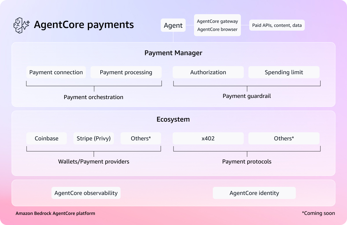
My most exciting news of last week: Amazon Bedrock AgentCore previewed the first managed payment capabilities enabling AI agents to autonomously access and pay for APIs, MCP servers, web content, and other agents. Built in partnership with Coinbase and Stripe, it removes the undifferentiated heavy lifting of building customized systems for billing, credential management, and compliance.

You can connect a Coinbase CDP wallet or Stripe Privy wallet as a payment connection, set session-level spending limits, and your agent transacts autonomously during execution. What excites me most is what AgentCore payments can unlock—like a research agent that can pay for real-time market data on the fly, or a coding agent calling paid APIs mid-task.

To learn more, visit the blog post, dive deeper using the documentation, and get started with the AgentCore CLI.

Last week’s launches
Here are last week’s launches that caught my attention:

  • Agent Toolkit for AWS – A production-ready suite of tools and guidance, available at no additional charge, that helps AI coding agents build on AWS with fewer errors, lower token costs, and enterprise-grade security controls. The Agent Toolkit for AWS is the successor to the MCP servers, plugins, and skills available on AWS Labs. To get started, visit the quick start guide or browse the available skills and plugins on GitHub.
  • AWS MCP Server GA – You can use a managed remote Model Context Protocol (MCP) server that gives AI agents and coding assistants secure, authenticated access to all AWS services through a small, fixed set of tools. It is part of the Agent Toolkit for AWS. To learn more, visit Seb Stormacq’s blog post.
  • Amazon WorkSpaces for AI agents (Preview) – You can use AI agents to securely access and operate desktop applications through managed WorkSpaces environments. This capability allows organizations to automate everyday workflows at scale while maintaining full enterprise-grade governance and compliance. To learn more, visit Micah Walter’s blog post.
  • Amazon EC2 M8idn/M8idb and R8idn/R8idb instances – These instances are powered by custom sixth-generation Intel Xeon Scalable processors available only on AWS and the latest sixth-generation AWS Nitro cards. These instances deliver up to 43% better compute performance per vCPU compared to previous-generation instances. M8idn/R8idn instances offer up to 600 Gbps network bandwidth, and M8idb/R8idb instances deliver up to 300 Gbps EBS bandwidth.

For a full list of AWS announcements, be sure to keep an eye on the What’s New with AWS page.

Additional updates
Here are some additional news items that you might find interesting:

  • Valkey turns two – Valkey stands as proof that open, community-driven technology innovates faster, scales further, and delivers more value than any single-vendor model. Valkey has surpassed 100 million Docker pulls (up 17x year over year) and attracted more than 225 contributors who have submitted over 1,500 pull requests, roughly double the development pace of Redis over the same period. You can also use the latest Valkey 9.0 in Amazon ElastiCache.
  • Query billion-scale vectors with SQL – You can learn how to query Amazon S3 Vectors from Amazon Aurora PostgreSQL-Compatible Edition using standard SQL, and how to combine vector similarity results with relational filters in a single query, for example, finding the most semantically similar products and then filtering by price, stock status, or tenant in one SQL statement.
  • Building an end-to-end agentic SRE using AWS DevOps Agent – Learn how to configure DevOps Agent Spaces that define an investigation scope, integrating seamlessly with Amazon CloudWatch, Splunk, GitHub, and Slack. You can also learn how to trigger automated investigations via webhooks, generate mitigation plans, and hand off agent-ready specs to coding agents like Kiro for implementation.

For a full list of AWS blog posts, be sure to keep an eye on the AWS Blogs page.

Learn more about AWS, browse and join upcoming AWS-led in-person and virtual events, startup events, and developer-focused events as well as AWS Summits and AWS Community Days. Join the AWS Builder Center to connect with builders, share solutions, and access content that supports your development.

That’s all for this week. Check back next Monday for another Weekly Roundup!

— Channy

Stenberg: Mythos finds a curl vulnerability

Post Syndicated from jzb original https://lwn.net/Articles/1072325/

Daniel Stenberg has published a lengthy
article
on his thoughts on Anthropic’s Mythos, which the company
decided was too dangerous for wide public release.

My personal conclusion can however not end up with anything else
than that the big hype around this model so far was primarily
marketing. I see no evidence that this setup finds issues to any
particular higher or more advanced degree than the other tools have
done before Mythos. Maybe this model is a little bit better, but even
if it is, it is not better to a degree that seems to make a
significant dent in code analyzing.

This is just one source code repository and maybe it is much better
on other things. I can only tell and comment on what it found
here.

But allow me to highlight and reiterate what I have said before: AI
powered code analyzers are significantly better at finding security
flaws and mistakes in source code than any traditional code analyzers
did in the past. All modern AI models are good at this now. Anyone
with time and some experimental spirits can find security problems
now. The high
quality chaos
is real.

[$] Providing 64KB base pages with 4KB kernels, two different ways

Post Syndicated from corbet original https://lwn.net/Articles/1071484/

Some CPU architectures are able to run with a number of different base-page
sizes; using a larger size can often result in better performance at the
cost of increased memory use. Other architectures are more limited. At
the 2026 Linux
Storage, Filesystem, Memory Management, and BPF Summit
, two sessions in
the memory-management track explored options for letting processes run with
64KB page sizes when the underlying kernel does not. The first was focused
on letting each process have its own page size, while the second concerned
bringing 64KB pages to x86 systems.

Debian to require reproducible builds

Post Syndicated from corbet original https://lwn.net/Articles/1072314/

Paul Gevers has slipped an interesting bit of news into a “bits from the release
team
” message:

Aided by the efforts of the Reproducible Builds project, we’ve
decided it’s time to say that Debian must ship reproducible
packages. Since yesterday, we have enabled our migration software
to block migration of new packages that can’t be reproduced or
existing packages (in testing) that regress in reproducibility.

As Gioele Barabucci pointed
out
, “reproducible” in this sense is limited to building within an
instance of Debian’s build environment, which is a tighter requirement than
is normally used. It is still a big step forward for reproducible builds.

Security updates for Monday

Post Syndicated from jzb original https://lwn.net/Articles/1072301/

Security updates have been issued by AlmaLinux (corosync, freeipmi, kernel, and kernel-rt), Debian (corosync, firefox-esr, kernel, lcms2, libpng1.6, linux-6.1, php8.2, php8.4, postorius, pyjwt, and tor), Fedora (dotnet10.0, exim, gnutls, kernel, nextcloud, nodejs22, php, proftpd, prosody, python-pulp-glue, python-requests, rclone, and SDL3_image), Mageia (firefox, nss, rootcerts, openvpn, thunderbird, and vim), Oracle (corosync, freeipmi, gstreamer1-plugins-bad-free, gstreamer1-plugins-base, and gstreamer1-plugins-good, kernel, libpng, and mingw-libtiff), Slackware (kernel and mozilla), SUSE (build, product-composer, c-ares, cairo, copacetic, distribution, firefox, firefox-esr, frr, glibc, go1.25, google-cloud-sap-agent, iproute2, java-11-openj9, java-17-openj9, java-17-openjdk, java-1_8_0-openj9, java-21-openj9, java-21-openjdk, java-25-openjdk, kernel, libexif-devel, libpcp-devel, libtpms, libtree-sitter0_26, Mesa, micropython, mozjs128, nginx, opencc, openCryptoki, php-composer2, podman, postfix, python-pytest, python311-Django, python311-Django4, redis, semaphore, strongswan, terraform-provider-aws, terraform-provider-azurerm, terraform-provider-external, terraform-provider-google, terraform-provider-helm, terraform-provider-kubernetes, terraform-provid, tor, valkey, vim, and wireshark), and Ubuntu (linux-nvidia-tegra, linux-raspi, linux-raspi-5.4, and nasm).

AI is not neutral: What recent research says about bias, identity, and power

Post Syndicated from Bonnie Sheppard original https://www.raspberrypi.org/blog/ai-is-not-neutral-what-recent-research-says-about-bias-identity-and-power/

Artificial intelligence (AI) systems are often presented as objective. But plenty of evidence shows that AI systems can reflect and reinforce existing inequalities, from healthcare and education to scientific research itself.

In the first seminar of our new research seminar series on applied AI, Thema Monroe-White from George Mason University explored how we can better understand — and challenge — these patterns. Her talk focused on race-conscious algorithmic approaches to AI and data, and what they reveal about how knowledge is produced, represented, and used.

Thema Monroe-White.
Thema Monroe-White is Associate Professor of Artificial Intelligence and Innovation Policy at the Schar School of Policy and Government and the Department of Computer Science (joint) at George Mason University.

Drawing on two large-scale studies in her seminar, Thema showed that both scientific research and AI systems are shaped by human identities and social structures, and that recognising this is essential for educators, researchers, and anyone working with data.

Who produces knowledge — and why that matters

A key idea running through Thema’s seminar was that data and algorithms are not neutral. They are shaped by the people, institutions, and systems that produce them.

Thema uses critical quantitative and intersectional approaches in her work to:

  • Challenge the misconception that computational methods are objective
  • Highlight how race and gender shape data and outputs
  • Examine how systems of power influence what gets measured, valued, and reproduced

Thema and her collaborators have been conducting research in this area for more than a decade, developing techniques that systematically measure bias and its impact on society. 

In a groundbreaking study published in 2022, just before the release of ChatGPT, Thema’s team used large-scale computational analysis of more than 5 million research articles to explore inequalities in scientific publishing. The data analysis approaches developed for this study were later used to explore bias in large language models (LLMs).

However, the 2022 study already demonstrated wide-reaching disparities in science and surfaced deep-rooted issues, showing that bias was already ingrained in the scientific data that was used to train LLM, and affecting topic choices, citation and institutional differences.

Identity and topic choice

The results showed clear inequalities in the relationship between identity and topic choice. Authors from marginalised groups were more likely to study topics related to their communities and lived realities, including topics such as racial disparities and discrimination. Gendered patterns also appeared, with women publishing more frequently on more feminised topics, including families, literacy, learning, nursing, and pregnancy.

Thema’s team demonstrated that there are clear differences in which topics are investigated and published by different groups. This has significant effects on which knowledge is available for public discourse and decision making.

Citation inequalities

The study also found citation inequalities. Even among authors studying the same topic, authors from some groups were cited less often than others, with black and Latinx women the least likely to be cited. This shows that inequality is not only present in what gets studied, but also in whose work is recognised.

Institutional context

Institutional context mattered too. Researchers at mission-driven institutions were more likely to publish on topics connected to marginalised communities, while scholars at institutions seen as elite were more likely to publish on topics that aligned more closely with dominant groups and norms.

Taken together, the findings point to a simple but important idea: who we are shapes what knowledge gets produced. That matters because when some groups are underrepresented in research, the topics that affect their lives may also be understudied.

What AI-generated stories reveal about bias

Having already developed their tool for name analysis for the previous study, Thema’s team was uniquely positioned to analyse the bias embedded in generative AI systems, specifically LLMs.

Thema’s most recent study examined how LLM–based tools represent people in everyday scenarios. The research team prompted the base models of LLM chatbots (such as Open AI’s ChatGPT, Anthropic’s Claude, Meta’s Llama, and Google’s PaLM or Gemini) to write short stories about students, workers, and relationships, generating 500,000 outputs across different domains. They then analysed how names associated with different racial and gender identities were portrayed.

AI-generated stories showed harmful stereotypes that can directly impact student performance.

One example Thema shared in the seminar described a student named “John” helping “Maria,” a student who had moved from Mexico and was struggling with Spanish. At first glance, this may seem like a small or even odd detail. But when oddities like this appear again and again across thousands of stories, they reveal systematic patterns.

The study found that characters with marginalised identities were more likely to be portrayed in subordinated roles in chatbot outputs. Characters with non-white-associated names were more often shown as needing help rather than offering it. Stereotypes were also reinforced, with some names repeatedly associated with struggling students, subordinate workers, or narrow professional roles. Some groups were omitted altogether, while white-associated names appeared more frequently and in more powerful positions.

A group of young people in a classroom

Similar biases appeared across stories related to education, work, and relationships. Across all three topics, the most common pattern was one in which white characters were more likely to lead, rescue, or mentor, while non-white characters were more likely to be helped, corrected, or spoken for.

For educators, this is especially important because many AI tools are now being introduced into classroom settings as writing assistants, tutors, or sources of personalised feedback. When these tools reproduce biases and unequal assumptions, they can shape not only what students read, but also how students see themselves and one another.

Towards more responsible AI tools and data practices

Rather than rejecting computational methods altogether, Thema argued for using them more thoughtfully and responsibly.

One approach she highlighted is the Wells-Du Bois protocol, a framework designed to support bias mitigation, transparency, and more reflective use of data and models. It encourages researchers and practitioners to think carefully about inadequate or biased data, identity proxies, subpopulation differences, and the kinds of harms that can arise when AI systems are used without sufficient context.

Underlying this is a broader principle: when we do not know enough, we should say so. And when systems affect marginalised communities, those communities should not be an afterthought in how we build, evaluate, or use technology.

What this means for your classroom

In her seminar, Thema emphasised the importance of thinking about how we respond to bias in AI tools in educational settings. Here are some starting points for meaningful discussions in your classroom:

  1. A good starting point is student agency. If AI tools are becoming part of students’ learning environments, then young people need opportunities to make informed choices about when and how to engage with them. That means not treating AI tool use as inevitable, and not assuming every student should want to use the tools in the same way. In some cases, empowering students may also mean making it clear that they can opt out.
  2. This also means helping learners ask better questions about the tools themselves. What leads to the kinds of bias we saw in these studies? What data were these systems trained on? Whose language, identities, and experiences are overrepresented, and whose are missing? Do the tools have access to student or classroom data, and if so, what are the implications?
  3. The seminar also points to the importance of resisting AI hype. In a rapidly changing landscape, it can be tempting to focus only on novelty, efficiency, or personalisation. But educators may want to take a longer-term view about AI technology use. What kinds of habits, dependencies, and expectations are these tools creating? Are they shifting students’ ideas about intelligence, creativity, or authority? What happens when biased outputs are repeated often enough to feel normal?
  4. Finally, the discussion around responsible use should include the wider costs of AI. Informing students about these tools should include not just potential benefits and risks, but also issues such as environmental impact and data use. A more balanced conversation can help prevent classroom discussions from reinforcing the hype that often surrounds AI.

If you would like to find out more about Thema’s work, you can find related materials on our seminar website.

You may also want to explore:

Join our next seminar

Our research seminars bring together educators and researchers to explore key questions in computing education.

Next in our series on applied AI, our Director of Research and Impact, Shuchi Grover, will talk about the role of K–12 education in developing competencies for the future of data and computing. Sign up now to join the seminar on 12 May, 17:00 BST:

The post AI is not neutral: What recent research says about bias, identity, and power appeared first on Raspberry Pi Foundation.

Final Countdown: Last Chance to Join the Rapid7 Global Cybersecurity Summit

Post Syndicated from Emma Burdett original https://www.rapid7.com/blog/post/it-last-chance-rapid7-global-cybersecurity-summit

The Rapid7 2026 Global Cybersecurity Summit is just around the corner, and with it, a final opportunity to join the conversations shaping how security teams are adapting to a rapidly changing landscape.

Over the past few weeks, we’ve shared a preview of what to expect, from the sessions and speakers to the themes running across the agenda. What has become increasingly clear is how closely these topics are connected. Security teams are being asked to move beyond reacting to incidents and instead understand how attacks begin, how they evolve, and how decisions can be made earlier with greater confidence.

What you will gain from attending

Across two days, the summit is structured to reflect how security teams actually operate. The first day builds a shared understanding of how the threat landscape has shifted, while the second day offers more focused sessions tailored to both leaders and practitioners.

Sessions such as The Reality of Running a SOC in 2026 and Inside the Modern SOC explore how attacks unfold in practice, following signals from initial access through to response. These discussions highlight how analysts interpret activity across identity, cloud, and endpoint environments, and how decisions are made when multiple signals compete for attention.

Other sessions, including Beyond the Vulnerability List and From Cloud Exposure to Runtime Attack, focus on how exposure is changing the way teams prioritize risk. The emphasis is on understanding context and how exposed assets actually are to attackers, helping teams determine which issues are most likely to lead to impact and where effort should be focused.

Alongside this, sessions like The AI Dilemma: Automating Defense Without Surrendering Judgment examine how AI is being applied within SOC workflows. The discussion moves beyond theory and looks at how teams are balancing automation with human oversight, ensuring that speed does not come at the expense of trust or accountability.

What’s changing for security teams right now

Security operations are evolving in response to changes in both attacker behavior and organizational complexity. Environments are more distributed, signals are more fragmented, and the time available to respond continues to shrink.

As a result, the focus is shifting toward earlier action, better prioritization, and more connected decision-making. This means linking exposure with detection, reducing unnecessary noise, and building workflows that allow teams to act with clarity when it matters most.

Across the summit, these ideas are explored from multiple perspectives, but they consistently point toward the same outcome. Teams that can connect context, visibility, and response are better positioned to reduce risk before it becomes an incident.

Secure your place

With the event approaching, this is the final opportunity to register and take part in these discussions. Whether you are responsible for strategy, operations, or day-to-day detection and response, the summit is designed to provide practical insights that can be applied immediately.

Join us on May 12–13 and see how security teams are putting these approaches into practice across real environments.

Register now

Строежите в Младост и красивите измамни картинки

Post Syndicated from Боян Юруков original https://yurukov.net/blog/2026/mladost-kartinki/

Районният кмет на Младост Ивайло Кукурин, който беше предложил да се застрои предимно общински имот със 75 метрова сграда, днес пусна визуализации какво всъщност е договорил с който трябва. Забелязах го от статията на citybuild.bg. Картинките изглеждат хубави, но още на пръв поглед се виждат проблемите с тях.

Надали някой ще бъде изненадан, но практически няма дърво на снимките му, което да е възможно въобще да е там. Първо „гората“ зад 75 метровата сграда вече е планирано да се застрои с 50 метрова сграда без никакво озеленяване съдейки по скиците. Второ, земята зад бл. 326 буквално до прозорците на живущите е очасти частна, а останалото вероятно ще бъде паркинг на въпросната спортна зала. Та нито едно дърво няма да остане там.

Второ, на картинките му не са отбелязани планираните пътища, които ще се изграждат на общинската земя и вече са отбелязани в isofmap. Не е отбелязана и сградата, която ще се строи точно до сегашния Lidl.

Трето, между картинките му има няколко несъответствия. На първата са сложили бл. 326 два пъти зад жълтата сграда, а в действителност там ще има паркинг. На втората пък липсва църквата. Както е нарисувана първоначално изглежда, че ще е на частен имот. Паркът нарисуван около нея също е върху частни имоти и вероятно ще бъдат застроени. Въобще, видимо е правено всичко с genai и без много мисъл дали отговаря на реалните планове. На общинската земя, отчасти заета от платения паркинг, някой някога е решил, че трябва да се сложи църква заемайки 1/3 от пространството при условие, че се вижда как цялото зелена площ наоколо ще бъде запечатана с бетон от край до край.

На снимките съм отбелязал в синьо къде са пътищата. В розово е отбелязана църквата, къде са частни имоти и ще се строи. Горе се виждат известните към този момент скици и обеми на сгради. В сиво се вижда одобреното от СОС по предложение на районният на Младост. В червено до него са двете сгради, които сега пуска като картинки. Вижда се, че отново въпреки критиките, 3D картата е доста точна години преди разрешението за строеж, макар и по-малко шарена от визуализациите на инвеститорите рекламирани от районния кмет. Долу снимките показват извадки от isofmap и собствеността на земята.

Утре, 12-ти май в 18:00 ще има протест пред районната община на Младост, в който живущите наоколо ще изразят недоволството си от това, което възприемат като презастрояване и претоварване на инфраструктурата на града.

The collective thoughts of the interwebz