On May 15, 2025, AWS unveiled a game-changing solution: AWS Transform for VMware. This innovative service tackles head-on the longstanding challenges of cloud migration, ushering in a new era of streamlined, efficient transitions to the AWS Cloud. By significantly reducing manual effort and accelerating the migration of critical VMware workloads, AWS Transform for VMware is set to revolutionize how organizations approach their cloud journey.
Since its general availability announcement, AWS Transform for VMware has ignited enthusiasm across industries, with organizations eager to leverage its capabilities to accelerate their VMware workload migration and modernization initiatives. As we dive into the intricacies of this transformative technology, we’ll uncover how AWS Transform for VMware is not just simplifying migrations, but reshaping the very landscape of cloud adoption and digital transformation.
The VMware migration challenge
Moving enterprise workloads to the cloud isn’t just a technical challenge – it’s a business transformation that demands precision, speed, and minimal disruption. Years of established operational processes have often led to complex environments with poorly documented configurations, inconsistent security practices, and heavy reliance on institutional knowledge. Technical teams must navigate intricate application dependencies, coordinate across multiple stakeholders, and maintain business continuity while executing these transformational projects. The lack of comprehensive documentation and clear understanding of system inter-dependencies frequently results in extended migration timelines and increased project risks. Additionally, the need to balance ongoing operations with migration activities presents challenges. Achieving proper knowledge transfer adds another layer of complexity to these critical initiatives.
Solution overview
Let’s explore how AWS Transform for VMware simplifies application discovery, automates network conversion, and orchestrates complex migrations through its comprehensive architecture in the following diagram.
To understand how these capabilities work together, let’s examine each component of the architecture.
Streamlined discovery and assessment
The journey begins with a thorough discovery and assessment of your VMware environment (1). AWS Transform for VMware (4) supports multiple discovery methods. One option is RVTools for VMware inventory collection. For customers running VMware NSX, there’s optional import/export functionality. Additionally, AWS Application Discovery Service offers both agent-based and agentless discovery options (2) to gather and collect data and dependencies for migration.
The Inventory Discovery capability (5) collects crucial data from your source environment and stores it securely in Amazon Simple Storage Service (Amazon S3) buckets (12) within the AWS Migration Discovery Account (7). This data forms the foundation for informed migration planning and is further processed by AWS Application Discovery Service (15) in the AWS Migration Planning Account. AWS Transform works together with these services to provide a single place to track migration progress and collect server inventory and dependency data, which is essential for successful application grouping and wave planning.
Intelligent network conversion and wave planning
With a comprehensive understanding of your environment, AWS Transform for VMware moves to the next critical phase. The Network Migration capability (19) automates the creation of AWS CloudFormation templates (13, 26) to set up the target network infrastructure. These templates ensure your cloud environment closely mirrors your source setup, simplifying the setup for the migration.
Meanwhile, the Wave Planning capability (6) uses advanced graph neural networks to analyze application dependencies and plan optimal migration waves. This minimizes complex portfolio and application dependency analysis, and provides ready-to-migrate wave plans, resulting in smooth migrations.
Enhanced security and compliance
Security remains paramount throughout the migration process. AWS Key Management Service (AWS KMS) (8, 16, 26) provides robust encryption for stored data, conversation history, and artifacts. By default, AWS managed keys are used, with the option to use customer managed keys (CMKs) for additional control.
AWS Organizations (9) enables centralized management across multiple AWS accounts, and AWS CloudTrail (14, 26) captures and logs API activities for a complete audit trail. Access control is managed through AWS Identity and Access Management (IAM) (26), providing centralized access management across AWS accounts.
Amazon CloudWatch (10, 26) continuously monitors AWS Transform service activities, resource utilization, and operational metrics within the management account, providing full visibility and control throughout the migration process. AWS Identity Center (11) further enhances security by providing centralized access management across all AWS accounts involved in the migration.
Orchestrated migration execution
When it’s time to execute the migration, AWS Transform orchestrates the end-to-end migration by coordinating across various AWS tools and services (20). The AWS Application Migration Service (25) replicates servers from your source environment to Amazon Elastic Compute Cloud (Amazon EC2) instances (21) in the AWS Migration Target Account (18), based on the carefully planned waves and groupings.
The AWS Replication Agent (2) works in tandem with AWS Application Migration Service to ensure efficient and reliable data transfer. Amazon Elastic Block Store (Amazon EBS) (21) provides the necessary storage for the migrated virtual machines, ensuring optimal performance and scalability.
Flexible network configuration
AWS Transform for VMware offers two networking models to suit different requirements:
Hub-and-spoke model – AWS Transit Gateway (23) connects virtual private clouds (VPCs) through a central hub VPC with shared NAT gateways. This model is ideal for centralized management and shared services.
Isolated model – Each VPC operates independently with no connectivity established. This approach is designed for customers with existing AWS network infrastructure, enabling you to manually connect the new VPCs to your existing network topology.
VPCs (22) created by AWS Transform match your on-premises network segments, providing a seamless transition. NAT gateways (24) provide outbound internet access for private subnets, maintaining security while enabling necessary connectivity. In hub-and-spoke architectures, centralized NAT gateways in the hub VPC can serve multiple spoke VPCs, optimizing costs and simplifying management. For isolated VPC deployments, dedicated NAT gateways must be provisioned within each VPC requiring internet access. In all cases, you must configure route tables to enable egress traffic flow through the NAT gateways
AWS Transform for VMware discovery workspaces are available globally (3). For the most up-to-date information on supported Regions, refer to AWS Services by Region (17).
Throughout the migration process, Amazon S3 buckets (12, 26) in both the AWS Migration Discovery Account and AWS Migration Target Account store key migration artifacts. These include inventory data, dependency mappings, wave plans, and application groupings, as well as Infrastructure as Code templates (AWS CloudFormation and AWS Cloud Development Kit) and per-wave migration plans.
Customers Benefits
AWS Transform for VMware delivers significant advantages:
Reduced manual effort – It minimizes human error and frees up valuable IT resources through automation
Enhanced accuracy – You can use AI-driven dependency mapping and wave planning for optimal migration strategies
Cost optimization – You can right-size instances and take advantage of AWS’s flexible pricing models for immediate and long-term savings
Future-proofing – It opens up the opportunity for ongoing modernization and innovation on the AWS Cloud platform
Always review and follow your organization’s security requirements, compliance obligations, and AWS security best practices when implementing any migration solution. For detailed security guidance, consult the AWS Security Documentation and your organization’s security team.
Pricing
AWS Transform accelerates migration and modernization projects for VMware workloads with agentic AI capabilities. Currently, we offer our core features—including assessment and transformation—at no cost* to AWS customers. This allows you to speed up your migration and modernization journey without upfront expenses.
*No cost refers to the AWS Transform service itself. Standard charges apply for AWS services and resources used during migrations.
Summary and Next Steps
AWS Transform for VMware empowers organizations to overcome the complexities of VMware migration and modernization. By providing a comprehensive, automated approach, it enables faster, more reliable transitions to the AWS Cloud. This new service offers the tools and capabilities needed to navigate the changing VMware landscape confidently.
The architecture we explored demonstrates how AWS Transform for VMware tackles key challenges:
Streamlines discovery and assessment processes
Automates network conversion and intelligent wave planning
Orchestrates migration execution with minimal disruption
Enhances security and compliance throughout the migration
Provides centralized management and monitoring
Offers flexible networking options to suit diverse requirements
Ready to accelerate your VMware migration journey? Visit the AWS Transform for VMware product page to learn more and get started today. Check out the following interactive demo of AWS Transform for VMware. If you’re exporting your network configuration from a VMware NSX environment, also refer to Exporting network configuration data with Import/Export for NSX. Our team of experts is ready to guide you through your migration and modernization initiatives, helping you unlock the full potential of the AWS Cloud.
To provide a seamless travel experience, aviation enterprises must streamline baggage handling to be as efficient as possible. Traditional baggage analytics systems often struggle with adaptability, real-time insights, data integrity, operational costs, and security, limiting their effectiveness in dynamic environments. Real-time analytics can help in several aspects, such as improving staffing decisions, baggage rerouting, payload planning, and predictive maintenance of Internet of Things (IoT) sensors and belt loaders.
Baggage management is a process that starts at baggage check-in and ends with the passenger claiming their baggage in a happy path scenario. The following figure explains the high-level baggage management process and respective key performance indicators (KPI). The illustration highlights the critical role of payload planning (part 1), baggage loading (part 2), and below wing payload closeout (part 3) in the flight departure process, all of which directly impact the flight on-time departure metric (part 4). Enhancing the KPIs associated with these essential steps is vital for airlines to optimize operations.
Figure 1: Baggage analytics KPIs
Common KPIs for baggage loading include baggage handling time, turnaround time impact, mishandled baggage rate, baggage accuracy rate, and baggage loading error rate. Similarly, the baggage check-in process plays a crucial role in enhancing the passenger experience. Analyzing variations in this metric across different stations and time periods provides valuable insights for identifying potential bottlenecks and improving efficiency.Airlines can measure performance KPIs using the following business process metrics:
Wait times – Wait times are the duration that a process step is waiting on an upstream dependency and are an important factor affecting the overall wait time. Analytics can help identify the potential areas (for example, stations, bag rooms, pier locations, belt loaders, or baggage types) where the processes and system can be fine-tuned to improve the overall wait time.
Error rate – Error rate is the time spent on correcting errors or defects. Within these processes, error rate is usually a result of data inconsistencies across multiple systems, manual data entries because of system unavailability or limited aircraft turn-around time, and inconsistencies between payload planning rules and loading procedures. Analytics can help classify these errors among system availability issues, outdated rules, inconsistent data between systems, and other factors. The classification can help prioritize fine-tuning and removing redundancies across systems, rules, and data.
Rework time – Rework time is time spent on correcting errors or defects. It can be improved but can’t be avoided, considering last-minute baggage, wheelchairs, ski equipment, and ship or aircraft changes that result in a new payload plan. Analytics can help classify the type, time, and frequency of rework activities across stations, staff members, baggage types, and scenarios related to flight delays and ship changes.
Cycle time – Cycle time is the time it takes to complete the process. You can improve the payload planning process cycle time by automating the payload distribution process. To do so, you need to identify and improve the time taken by the payload planning, loading, and closeout processes to reduce the complete departure process cycle time. In many cases, you can improve cycle time by adjusting the processes and adding extra resources, such as workforce, or in other cases by introducing automation. Analytics can identify these time-consuming steps and can be extended to use predictive models to apply mitigation strategies.
Traditional baggage analytics
As explained in the following figure, the traditional baggage handling solution uses monolithic databases with several upstream and downstream dependencies. Upstream dependencies include bags, flight and passenger event feeds to subscribe to the real-time changes in flight, checked bags, and passenger itinerary changes. Downstream dependencies include staffing and customer notifications. The core application interfaces include belt loaders, IoT devices, kiosks, handheld scanners, and web applications for monitoring and reporting. The airline typically stores the reports in the operational database referred to in the diagram as baggage handling (relational database), retaining historical data spanning multiple years, and makes them available to all personnel on the airline’s network. The traditional approach to baggage analytics entails nightly processing of data batches into an enterprise data warehouse (EDW) to generate performance metrics related to airlines’ baggage handling processes.
Figure 2: Traditional baggage analytics
Need for modernization
Modernizing baggage analytics is crucial for airlines to achieve growth and enhance operational efficiency. Key factors influencing the modernization are as follows:
Inefficiencies in near real-time decision-making – Current systems can’t process and analyze data in real time, leading to delayed responses to operational issues. Integration and data silos hinder insights, preventing proactive decision-making on baggage handling, routing, and anomaly detection.
Limitations of traditional ETL solutions – Legacy extract, transform, and load (ETL) processes are batch-driven, slow, and resource-intensive, making them unsuitable for dynamic airline operations. High maintenance costs and frequent failures reduce system reliability and availability.
Challenges in proactive anomaly detection and resolution during irregular operations – Airlines struggle to anticipate baggage issues during irregular operations, such as flight delays and weather disruptions. Without predictive analytics, preemptive actions remain a challenge in optimizing staffing, reducing mishandled baggage, and enhancing operational efficiency.
Solution
The modernization of baggage operations must include breaking down the monolithic database into distinct databases based on business capabilities to address performance bottlenecks. Business capabilities can be described as fundamental abilities or competencies that a business possesses and that enable it to achieve its objectives and deliver value to its customers.
As explained in the following figure, the business capabilities for baggage management can be defined as baggage acceptance (check-in), baggage loading, baggage offloading, baggage tracking, baggage mishandling and claims, baggage rerouting, and more. [part 1]. The solution proposes Amazon DynamoDB for an operational database across all baggage management capabilities. DynamoDB global tables provide 99.999% availability with near-zero Recovery Time Objective (RTO) and Recovery Point Objective (RPO), which is crucial for mission-critical baggage handling systems. More details related to baggage operational database modernization can be found at Enhance the reliability of airlines’ mission-critical baggage handling using Amazon DynamoDB in the AWS Database Blog.
The proposed logical solution for baggage operational analytics suggests segregating operational data from historical data, referred to in the diagram as baggage analytics and historical reporting database, to enhance efficiency and alleviate the burden on the operational database [part 3].
Figure 3: Modern baggage analytics
The solution further uses streaming architecture for the ongoing transfer of data from the operational database to the baggage analytics and historical reporting database [part 2]. This approach aims to facilitate near real-time analytics.The key features for a robust streaming architecture include:
Low-latency processing to enable near real-time updates
Scalability and elasticity to handle dynamic workloads efficiently
Fault tolerance and durability to promote data reliability with replication
The ability for multiple consumers to process the same data in parallel at full speed without bottlenecks or interference
Exactly one-time processing to avoid duplication and maintain data integrity
In this architecture, Kinesis Data Streams is selected to enable fan-out to multiple downstream consumers, extended data retention, and integration with Amazon Managed Service for Apache Flink. Amazon Managed Service for Apache Flink performs stateful stream processing—such as windowed aggregation, filtering, and anomaly detection—before passing data to DynamoDB or Aurora for further analytical aggregation and reporting. Although DynamoDB Streams could also have been used, Kinesis Data Streams provides greater flexibility and throughput for the scale of event processing required here. Additionally, Kinesis Data Streams data retention allows message replays for improved reliability and analysis.
Baggage analytics on AWS Cloud
The solution will use Amazon Simple Storage Service (Amazon S3) for structured and unstructured data storage and Amazon Aurora PostgreSQL-Compatible Edition for relational aggregations. Aurora is well-suited for handling complex aggregations across multiple dimensions (such as month, year, station, and shift) with efficient indexing and SQL functions optimized for reporting. Its relational capabilities support analytical queries needed for performance metrics while providing scalability and efficiency
The following figure explains the high-level cloud architecture for baggage analytics using AWS services.
Figure 4: Near real-time baggage analytics architecture on AWS
The solution can support the following analytics:
Interactive and investigative analytics which can produce charts and graphs and discover patterns and anomalies in the baggage data used by product owners. The solution proposes using Amazon QuickSight, which is an interactive tool. Additionally, the solution proposes Amazon Q in QuickSight for natural language queries using a chat-based interface. Amazon QuickSight can be configured using an AWS Glue crawler to automatically discover and extract metadata from various data stores such as Amazon S3 and Amazon Aurora and catalog it in a centralized repository. Amazon QuickSight can be configured to use Amazon Athena to read the data catalog.
Predictive analytics used by data scientists involves analyzing historical data to predict future events or behaviors. It uses statistical algorithms and machine learning (ML) techniques to forecast outcomes. The proposed solution is to use a SageMaker notebook to perform predictive analytics on baggage data.
Conclusion
Cloud-based solutions such as Kinesis Data Streams, Athena, and QuickSight revolutionize baggage analytics with scalable, cost-effective infrastructure. By integrating real-time data streaming, analysis, and visualization, they eliminate data silos and enable data-driven decision-making.This modernization optimizes processes, proactively resolving issues to minimize passenger disruptions. Embracing cloud-powered analytics isn’t just a necessity but a strategic step toward greater efficiency, resilience, and customer satisfaction.With this solution, airlines can enhance preemptive issue resolution in baggage operations. Real-time analytics enables better workforce planning, allowing airlines to predict staffing needs at departure and arrival stations, reducing labor costs while ensuring smooth operations. Additionally, data-driven insights help identify inefficiencies during irregular operations, enabling informed decisions for traffic diversion and process optimization.
IBM Consulting is an AWS Premier Tier Services Partner that helps customers who use AWS to harness the power of innovation and drive their business transformation. They are recognized as a Global Systems Integrator (GSI) for over 22 competencies, including travel and hospitality consulting. For more information, please contact an IBM Representative.
About the authors
Neeraj Kaushik is an Open Group Certified Distinguish Architect at IBM with two decades of experience in client-facing delivery roles. His experience spans several industries, including travel and transportation, banking, retail, education, healthcare, and anti-human trafficking. As a trusted advisor, he works directly with the client executive and architects on business strategy to define a technology roadmap. As a hands-on Chief Architect AWS Professional Certified Solution Architect, AWS Certified Machine Learning Specialist and Natural Language Processing Expert, he has led multiple complex cloud modernization programs and AI initiatives.
Jay Pandya is a Senior Partner Solutions Architect in the Global Systems Integrator (GSI) team at Amazon Web Services (AWS). He has over 30 years of IT experience and is helping and providing guidance to AWS GSI partners to build, design, and architect agile, scalable, highly available, and secure solutions on AWS. Outside of the office, Jay enjoys spending time with his family and traveling, and he is an aviation enthusiast and avid sports and Formula 1 fan.
Vijay Gokarn is a Senior Solution Architect at IBM with extensive experience across industries including financial services, healthcare, industrial, retail, and travel and hospitality. He leads complex AWS transformation initiatives, drawing on his hands-on expertise as an AWS Certified Solutions Architect Associate. Vijay specializes in serverless architectures, event-driven systems, and enterprise modernization. As a skilled architect and team leader, he has delivered impactful solutions in cloud modernization, digital banking, and intelligent automation. His passion lies in bridging business strategy with technical execution to drive scalable digital transformation.
Subhash Sharma is Sr. Partner Solutions Architect at AWS. He has more than 25 years of experience in delivering distributed, scalable, highly available, and secured software products using Microservices, AI/ML, the Internet of Things (IoT), and Blockchain using a DevSecOps approach. In his spare time, Subhash likes to spend time with family and friends, hike, walk on beach, and watch TV.
Versions v2.43.7, v2.44.4, v2.45.4, v2.46.4, v2.47.3, v2.48.2, v2.49.1 and
v2.50.1 of the Git source-code management system have been released.
“This is a set of coordinated security fix releases. Please update at
your earliest convenience“. See the announcement for details;
many of the vulnerabilities have to do with tricks buried in untrusted
repositories.
Version
140 of the Thunderbird mail client has been released. Notable
features include “dark message mode” to adapt message content
to dark mode, the ability to easily transfer desktop
settings to the mobile Thunderbird client, experimental support for
Microsoft Exchange, as well as global controls for message threading
and sort order.
Thunderbird 140 is an extended-support
release (ESR) which will be supported for 12 months. However, the
Thunderbird project is trying to encourage users to adopt the Release
channel for monthly updates instead. The project is staggering
upgrades to 140 for existing Thunderbird users in order to catch any
significant bugs before they are widely deployed, but users can
upgrade manually via the Help > About
menu. See the release
notes for a full list of changes.
Amazon Web Services (AWS) is pleased to announce that three new AWS services have been added to the scope of our Payment Card Industry Data Security Standard (PCI DSS) certification:
This certification means that customers can use these services while maintaining PCI DSS compliance, enabling innovation without compromising security. The full list of services can be found on the AWS Services in Scope by Compliance Program page. The PCI DSS compliance package includes two key components:
Attestation of Compliance (AOC) – demonstrates that AWS was successfully validated against the PCI DSS standard.
AWS Responsibility Summary – provides guidance to help AWS customers understand their responsibility in developing and operating a highly secure environment on AWS for handling payment card data.
AWS was evaluated by Coalfire, a third-party Qualified Security Assessor (QSA).
This refreshed certification offers customers greater flexibility in deploying regulated workloads while reducing compliance overhead. Customers can access the PCI DSS reports through AWS Artifact. This self-service portal provides on-demand access to AWS compliance reports, streamlining audit processes.
To learn more about our PCI programs and other compliance and security programs, see the AWS Compliance Programs page. As always, we value your feedback and questions; reach out to the AWS Compliance team through the Compliance Support page.
If you have feedback about this post, submit comments in the Comments section below. If you have questions about this post, contact AWS Support.
At Cloudflare, PostgreSQL and ClickHouse are our standard databases for transactional and analytical workloads. If you’re part of a team building products with configuration in our Dashboard, chances are you’re using PostgreSQL. It’s fast, versatile, reliable, and backed by over 30 years of development and real-world use. It has been a foundational part of our infrastructure since the beginning, and today we run hundreds of PostgreSQL instances across a wide range of configurations and replication setups.
ClickHouse is a more recent addition to our stack. We started using it around 2017, and it has enabled us to ingest tens of millions of rows per second while supporting millisecond-level query performance. ClickHouse is a remarkable technology, but like all systems, it involves trade-offs.
In this post, I’ll explain why we chose TimescaleDB — a Postgres extension — over ClickHouse to build the analytics and reporting capabilities in our Zero Trust product suite.
Designing for future growth
After a decade in software development, I’ve grown to appreciate systems that are simple and boring. Over time, I’ve found myself consistently advocating for architectures with the fewest moving parts possible. Whenever I see a system diagram with more than three boxes, I ask: Why are all these components here? Do we really need all of this?
As engineers, it’s easy to fall into the trap of designing for scenarios that might never happen. We imagine future scale, complex failure scenarios, or edge cases, and start building solutions for them upfront. But in reality, systems often don’t grow the way we expect, or don’t have to. Designing for large scale can be deferred by setting the right expectations with customers, and by adding guardrails like product limits and rate limits. Focusing on launching initial versions of products with just a few essential parts, maybe two or three components, gives us something to ship, test, and learn from quickly. We can always add complexity later, but only once it’s clear we need it.
Whether I specifically call it YAGNI, or Keep it simple, stupid, or think about it as minimalism in engineering, the core idea is the same: we’re rarely good at predicting the future, and every additional component we introduce carries a cost. Each box in the system diagram is something that can break itself or other boxes, spiral into outages, and ruin weekend plans of on-call engineers. Each box also requires documentation, tests, observability, and service level objectives (SLOs). Oftentimes, teams need to learn a new programming language just to support a new box.
Making Digital Experience Monitoring simple
Two years ago, I was tasked with building a new product at Cloudflare: Digital Experience Monitoring (DEX). DEX provides visibility into device, network, and application performance across Zero Trust environments. Our initial goal was clear — launch an MVP focused on fleet status monitoring and synthetic tests, giving customers actionable analytics and troubleshooting. From a technical standpoint, fleet status and synthetic tests are two types of structured logs generated by the WARP client. These logs are uploaded to an API, stored in a database, and ultimately visualized in the Cloudflare Dashboard.
As with many new engineering teams at Cloudflare, DEX started as a “tiger team”: a small group of experienced engineers tasked with validating a new product quickly. I worked with the following constraints:
Team of three full-stack engineers.
Daily collaboration with 2-3 other teams.
Can launch in beta, engineering can drive product limits.
Emphasis on shipping fast.
To strike a balance between usefulness and simplicity, we made deliberate design decisions early on:
Fleet status logs would be uploaded from WARP clients at fixed 2-minute intervals.
Synthetic tests required users to preconfigure them by target (HTTP or traceroute) and frequency.
We capped usage: each device could run up to 10 synthetic tests, no more than once every 5 minutes.
Data retention of 7 days.
These guardrails gave us room to ship DEX months earlier and gather early feedback from customers without prematurely investing in scalability and performance.
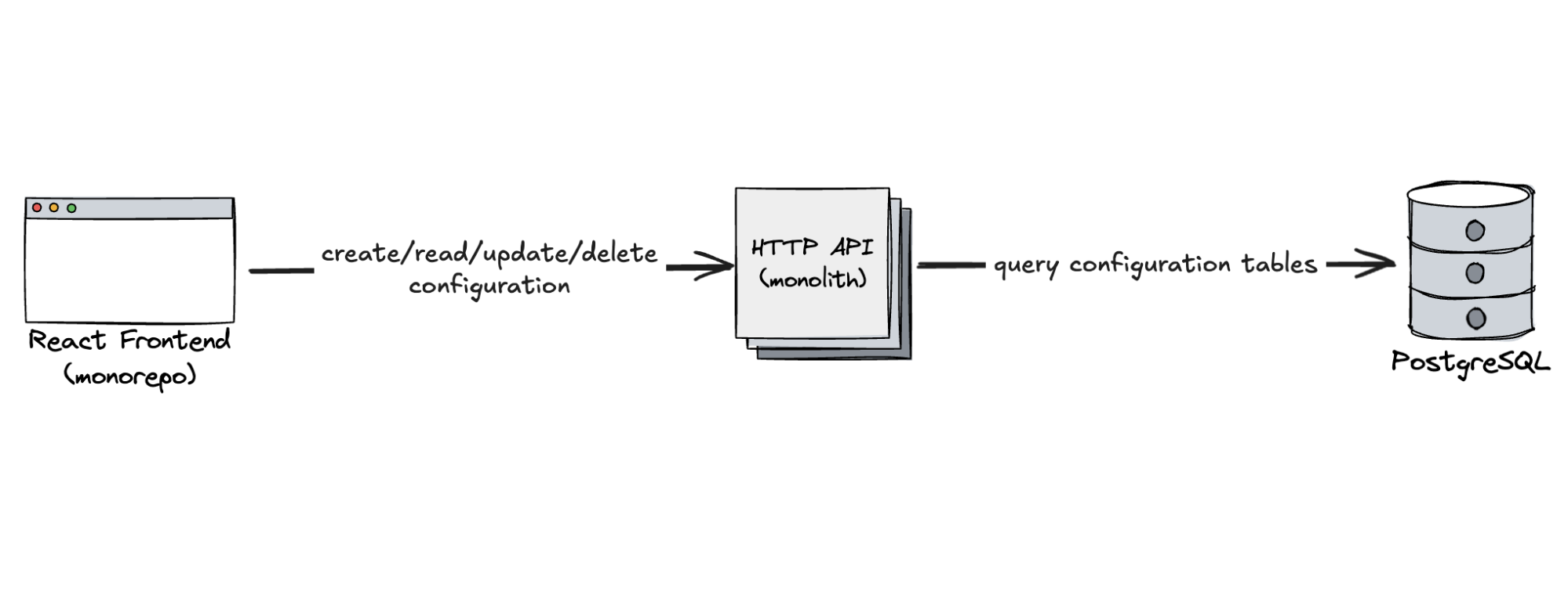
We knew we needed a basic configuration plane — an interface in the Dashboard for users to create and manage synthetic tests, supported by an API and database to persist this data. That led us to the following setup:
HTTP API for managing test configurations.
PostgreSQL for storing those configurations.
React UI embedded in the Cloudflare Dashboard.
Just three components — simple, focused, and exactly what we needed. Of course, each of these boxes came with real complexity under the hood. PostgreSQL was deployed as a high-availability cluster: one primary, one synchronous replica for failover scenarios, and several asynchronous replicas distributed across two geographies. The API was deployed on horizontally scaled Kubernetes pods across two geographies. The React app was served globally as standard via Cloudflare’s network. Thanks to our platform teams, all of that complexity was abstracted away, allowing us to think in terms of just three essential parts, but it really shows that each box can come with a huge cost behind the scenes.
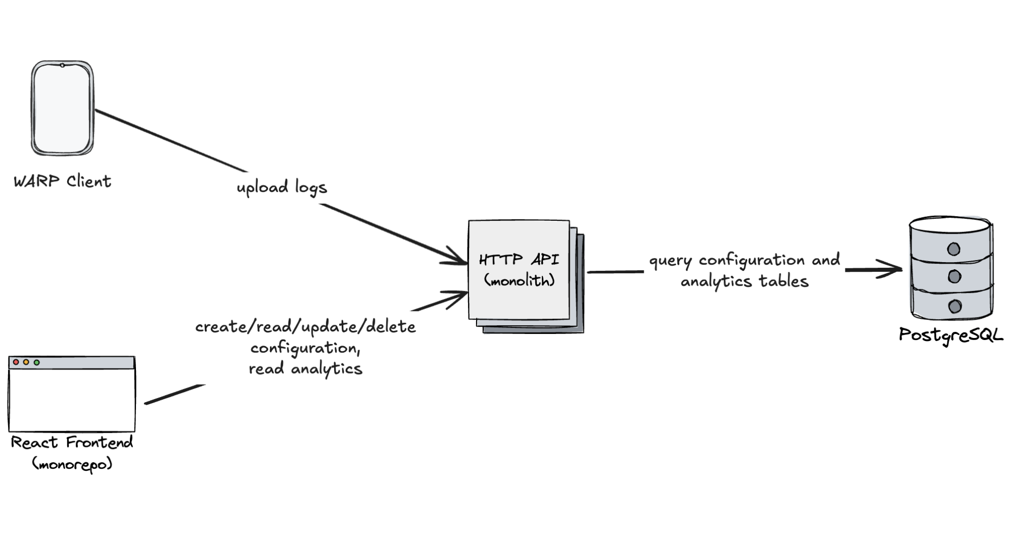
Next, we needed to build the analytics plane — an ingestion pipeline to collect structured logs from WARP clients, store them, and visualize them for our customers in the Dashboard. I was personally excited to explore ClickHouse for this. I have seen its performance in other projects and was eager to experiment with it. But as I dug into the internal documentation on how to get started with ClickHouse, reality set in:
Writing data to Clickhouse
Your service must generate logs in a clear format, using Cap’n Proto or Protocol Buffers. Logs should be written to a socket for logfwdr to transport to PDX, then to a Kafka topic. Use a Concept:Inserter to read from Kafka, batching data to achieve a write rate of less than one batch per second.
Oh. That’s a lot. Including ClickHouse and the WARP client, we’re looking at five boxes to be added to the system diagram. This architecture exists for good reason, though. The default and most commonly used table engine in ClickHouse, MergeTree, is optimized for high-throughput batch inserts. It writes each insert as a separate partition, then runs background merges to keep data manageable. This makes writes very fast, but not when they arrive in lots of tiny batches, which was exactly our case with millions of individual devices uploading one log event every 2 minutes. Too many small writes can trigger write amplification, resource contention, and throttling.
So it became clear that ClickHouse is a sports car and to get value out of it we had to bring it to a race track, shift into high gear, and drive it at top speed. But we didn’t need a race car — we needed a daily driver for short trips to a grocery store. For our initial launch, we didn’t need millions of inserts per second. We needed something easy to set up, reliable, familiar, and good enough to get us to market. A colleague suggested we just use PostgreSQL, quoting “it can be cranked up” to handle the load we were expecting. So, we took the leap!
First design of configuration and analytics plane for DEX:
Using PostgreSQL for analytics
Structurally, there’s not much difference between configuration data and analytical logs. Logs are simply structured payloads — often in JSON — that can be transformed into a columnar format and persisted in a relational database.
To store these logs, we created a simple PostgreSQL table:
CREATE TABLE device_state (
	"timestamp" TIMESTAMP WITH TIME ZONE NOT NULL,
	account_id TEXT NOT NULL,
	device_id TEXT NOT NULL,
	colo TEXT,
	status TEXT,
	mode TEXT,
	client_version TEXT,
	client_platform TEXT
);
You might notice that this table doesn’t have a primary key. That’s intentional, because time-series data is almost never queried by a unique ID. Instead, we query by time ranges and filter by various attributes (e.g. account ID or device ID). Still, we needed a way to deduplicate logs in case of client retries.
We created two indexes to optimize for our most common queries:
CREATE UNIQUE INDEX device_state_device_account_time ON device_state USING btree (device_id, account_id, “timestamp”);
CREATE INDEX device_state_account_time ON device_state USING btree (account_id, “timestamp”);
The unique index ensures deduplication: each (device, account, timestamp) tuple represents a single, unique log. The second index supports typical time-window queries at the account level. Since we always query by account_id (represents individual customers) and timestamp, they are always a part of the index.
We inserted data from our API using UPSERT query:
INSERT INTO device_state (…) VALUES (…) ON CONFLICT DO NOTHING;
About order of columns in multicolumn indexes
PostgreSQL’s B-tree indexes support multiple columns, but column order has a major impact on query performance.
A multicolumn B-tree index can be used with query conditions that involve any subset of the index’s columns, but the index is most efficient when there are constraints on the leading (leftmost) columns. The exact rule is that equality constraints on leading columns, plus any inequality constraints on the first column that does not have an equality constraint, will be used to limit the portion of the index that is scanned. Constraints on columns to the right of these columns are checked in the index, so they save visits to the table proper, but they do not reduce the portion of the index that has to be scanned.
What’s interesting in time series workloads is that the queries usually have inequality constraints on the time column, and then equality constraints on all other columns.
A typical query to build line charts and pie charts visualizing data in a time interval often looks like this:
SELECT
  DATE_TRUNC(‘hour’, timestamp) as hour,
  account_id,
  device_id,
  status,
  COUNT(*) as total
FROM device_state
WHERE
  account_id = ‘a’ AND
  device_id = ‘b’ AND
  timestamp BETWEEN ‘2025-07-01’ AND ‘2025-07-02’
GROUP BY hour, account_id, device_id, status;
Notice our WHERE clause — it has equality constraints on account_id and device_id, and two inequality constraints on timestamp. If we had built our index in the order of (timestamp, account_id, device_id), only the “timestamp” section of the index could’ve been used to reduce the index section to be scanned, and account_id and device_id would have to be fully scanned, with values that are not ‘a’ or ‘b’ filtered out after scanning.
Additionally, the runtime complexity of search in btree is O(log n) — the search will get slower as the size of your table (and all indexes) grows, so another optimization is to reduce the portion of the index that needs to be scanned. Even for columns with equality constraints, you can greatly reduce query times by ordering columns by cardinality. We’ve seen up to 100% improvement in SELECT query performance when we simply changed the order of account_id and device_id in our multicolumn index.
To get the best performance for time range queries, we follow these rules for order of columns:
The timestamp column is always last.
Other columns are leading columns, ordered by their cardinalities starting with the highest cardinality column.
Launch and improvements
Because we took a step back during system design and avoided optimizing for the future, thanks to our minimal and focused architecture, we went from zero to a working DEX MVP in under four months.
Early metrics were promising, providing reasonable throughput capabilities and latency for API requests:
~200 inserts/sec at launch.
Query latencies in the hundreds of milliseconds for most customers.
Post-launch, we focused on collecting feedback while monitoring system behavior. As adoption grew, we scaled to 1,000 inserts/sec, and our tables grew to billions of rows. That’s when we started to see performance degradation — particularly for large customers querying 7+ day time ranges across tens of thousands of devices.
Optimizing query performance with precomputed aggregates
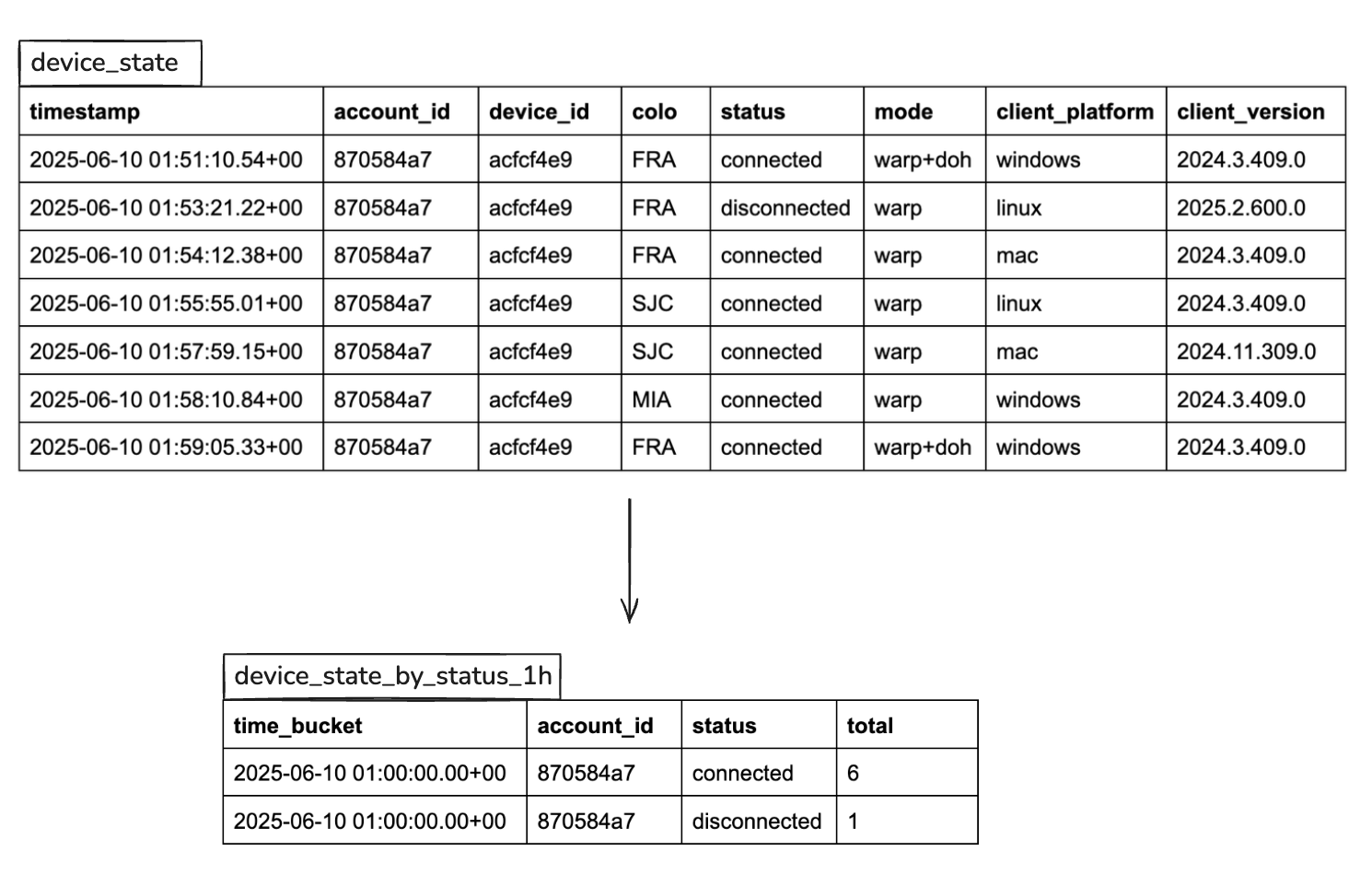
As DEX grew to billions of device logs, one of the first performance optimizations we explored was precomputing aggregates, also known as downsampling.
The idea is that if you know the shape of your queries ahead of time — say, grouped by status, mode, or geographic location — you can precompute and store those summaries in advance, rather than querying the raw data repeatedly. This dramatically reduces the volume of data scanned and the complexity of the query execution.
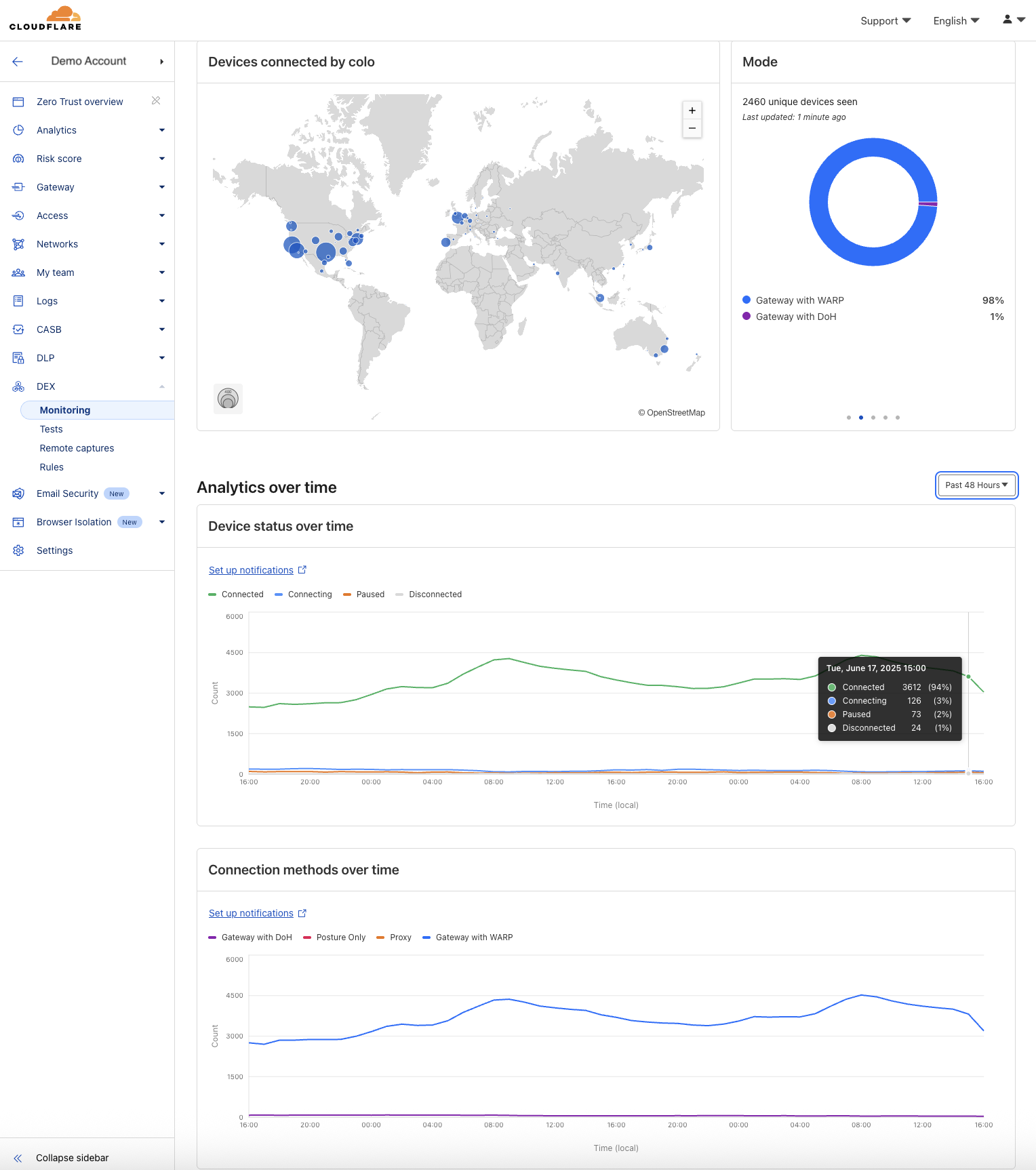
To illustrate this in an example, let’s consider DEX Fleet Status:
In our DEX Fleet Status dashboard, we render common visualizations like:
Number of connected devices by data center location (colo)
Device status and connection mode over time
These charts typically group logs by status, mode, or colo, either over a 1-hour window or across the full time range.
Our largest customers may have 30,000+ devices, each reporting logs every 2 minutes. That’s millions of records per day per customer. But the columns we’re visualizing (e.g. status and mode) only have a few distinct values (4–6). By aggregating this data ahead of time, we can collapse millions of rows into a few hundred per interval and query dramatically smaller, narrower tables.
This made a huge impact: we saw up to 1000x query performance improvement and charts that previously took several seconds now render instantly, even for 7-day views across tens of thousands of devices.
Implementing this technique in PostgreSQL is challenging. While PostgreSQL does support materialized views, they didn’t fit our needs out of the box because they don’t refresh automatically and incrementally. Instead, we used a cron job that was periodically running custom aggregation queries for all pre-aggregate tables (we had 6 of them). Our Database platform team had a lightweight framework built for data retention purposes that we plugged into. Still, any schema change required cross-team coordination, and we invested considerable time in optimizing aggregation performance. But the results were worth it: fast, reliable queries for the majority of customer use cases.
Table partitioning
Pre-computed aggregates are great, but they’re not the answer to everything. As we were adding more table columns for new DEX features, we needed to invest time in creating new pre-aggregated tables. Additionally, some features required queries with combined filters, which required querying the raw data that included all the columns. But we didn’t have good enough performance in raw tables.
One technique we considered to improve performance on raw tables was table partitioning. In PostgreSQL, tables are stored in one large file (large tables are split to 1 GB segment files). With partitioning, you can break a large table into smaller child tables, each covering a slice of data (e.g. one day of logs). PostgreSQL then scans only the relevant partitions based on your query’s timestamp filter. This can dramatically improve query performance in some cases.
What was particularly interesting for us was range-partitioning on the timestamp column, because our customers wanted longer data retention, up to one year, and storing one year of data in one large table would have destroyed query performance.
CREATE TABLE device_state (
    …
) PARTITION BY RANGE (timestamp);

CREATE TABLE device_state_20250601 PARTITION OF device_state
    FOR VALUES FROM ('2025-06-01') TO ('2025-06-02');
CREATE TABLE device_state_20250601 PARTITION OF device_state
    FOR VALUES FROM ('2025-06-02') TO ('2025-06-03');
CREATE TABLE device_state_20250601 PARTITION OF device_state
    FOR VALUES FROM ('2025-06-03') TO ('2025-06-04');
Unfortunately, PostgreSQL doesn’t automatically manage partitions — you must manually create each one as shown above, so we would have needed to build a full partition management system to automate this.
We ended up not adopting it because in the end, partitioning didn’t solve our core problem: speeding up frequent dashboard queries on recent raw data up to past 7 days.
TimescaleDB
As our raw PostgreSQL setup began to show its limits, we started exploring other options to improve query performance. That’s when we discovered TimescaleDB. What particularly caught my attention was columnstore and sparse indexes, common techniques in OLAP databases like ClickHouse. It seemed to be the solution for our raw performance problem. On top of that:
It’s Postgres: TimescaleDB is packaged as a PostgreSQL extension and it seamlessly coexists with it, granting access to the entire Postgres ecosystem. We can still use vanilla Postgres tables for transactional workloads, and TimescaleDB hypertables for analytical tasks, offering convenience of one database for everything.
Automatic partition management: Unlike Postgres, which requires manualtable partitioning, TimescaleDB’s hypertables are partitioned by default and automatically managed.
Automatic data pre-aggregation/downsampling: Tedious processes in native Postgres, such as creating and managing downsampled tables, are automated in TimescaleDB through continuous aggregates. This feature eliminates the need for custom-built cron jobs and simplifies the development and deployment of pre-computed aggregates.
Realtime data pre-aggregation/downsampling: A common problem with async aggregates is that they can be out-of-date, because aggregation jobs can take a long time to complete. TimescaleDB addresses the issue of outdated async aggregates with its realtime aggregation by seamlessly integrating the most recent raw data into rollup tables during queries.
Compression: Compression is a cornerstone feature of TimescaleDB. Compression can reduce table size by more than 90% while simultaneously enhancing query performance.
Columnstore performance for real-time analytics: TimescaleDB’s hybrid row/columnar engine, Hypercore, enables fast scans and aggregations over large datasets. It’s fully mutable, so we can backfill with UPSERTs. Combined with compression, it delivers strong performance for analytical queries while minimizing storage overhead.
One especially compelling aspect: TimescaleDB made aggregation and data retention automatic, allowing us to simplify our infrastructure and remove a box from the system architecture entirely.
Evaluating TimescaleDB for DEX
We deployed a self-hosted TimescaleDB instance on our canary PostgreSQL cluster to run an apples-to-apples comparison against vanilla Postgres. Our production backend was dual-writing to both systems.
As expected, installing TimescaleDB was trivial. Simply load the library and run the following SQL query:
CREATE EXTENSION IF NOT EXISTS timescaledb;
Then we:
Created raw tables
Converted them to hypertables
Enabled columnstore features
Set up continuous aggregates
Configured automated policies for compression and retention
Here’s a condensed example for device_state logs:
– Create device_state table.
CREATE TABLE device_state (
	…
);

– Convert it to a hypertable.
SELECT create_hypertable ('device_state', by_range ('timestamp', INTERVAL '1 hour'));

– Add columnstore settings
ALTER TABLE device_state SET (
    timescaledb.enable_columnstore,
    timescaledb.segmentby = ‘account_id’
);

– Schedule recurring compression jobs
CALL add_columnstore_policy(‘device_state’, after => INTERVAL '2 hours', schedule_interval => INTERVAL '1 hour');

– Schedule recurring data retention jobs
SELECT add_retention_policy(‘device_state’, INTERVAL '7 days');

– Create device_state_by_status_1h continuous aggregate
CREATE MATERIALIZED VIEW device_state_by_status_1h
WITH (timescaledb.continuous) AS
SELECT
  time_bucket (INTERVAL '1 hour', TIMESTAMP) AS time_bucket,
  Account_id,
  Status,
  COUNT(*) as total
FROM device_state
GROUP BY 1,2,3
WITH no data;

– Enable realtime aggregates
ALTER MATERIALIZED VIEW ‘device_state_by_status_1h’
SET (timescaledb.materialized_only=FALSE);

– Schedule recurring continuous aggregate jobs to refresh past 10 hours every 10 minutes
SELECT add_continuous_aggregate_policy (
  ‘device_state_by_status_1h’,
  start_offset=>INTERVAL '10 hours',
  end_offset=>INTERVAL '1 minute',
  schedule_interval=>INTERVAL '10 minutes',
  buckets_per_batch => 1
);
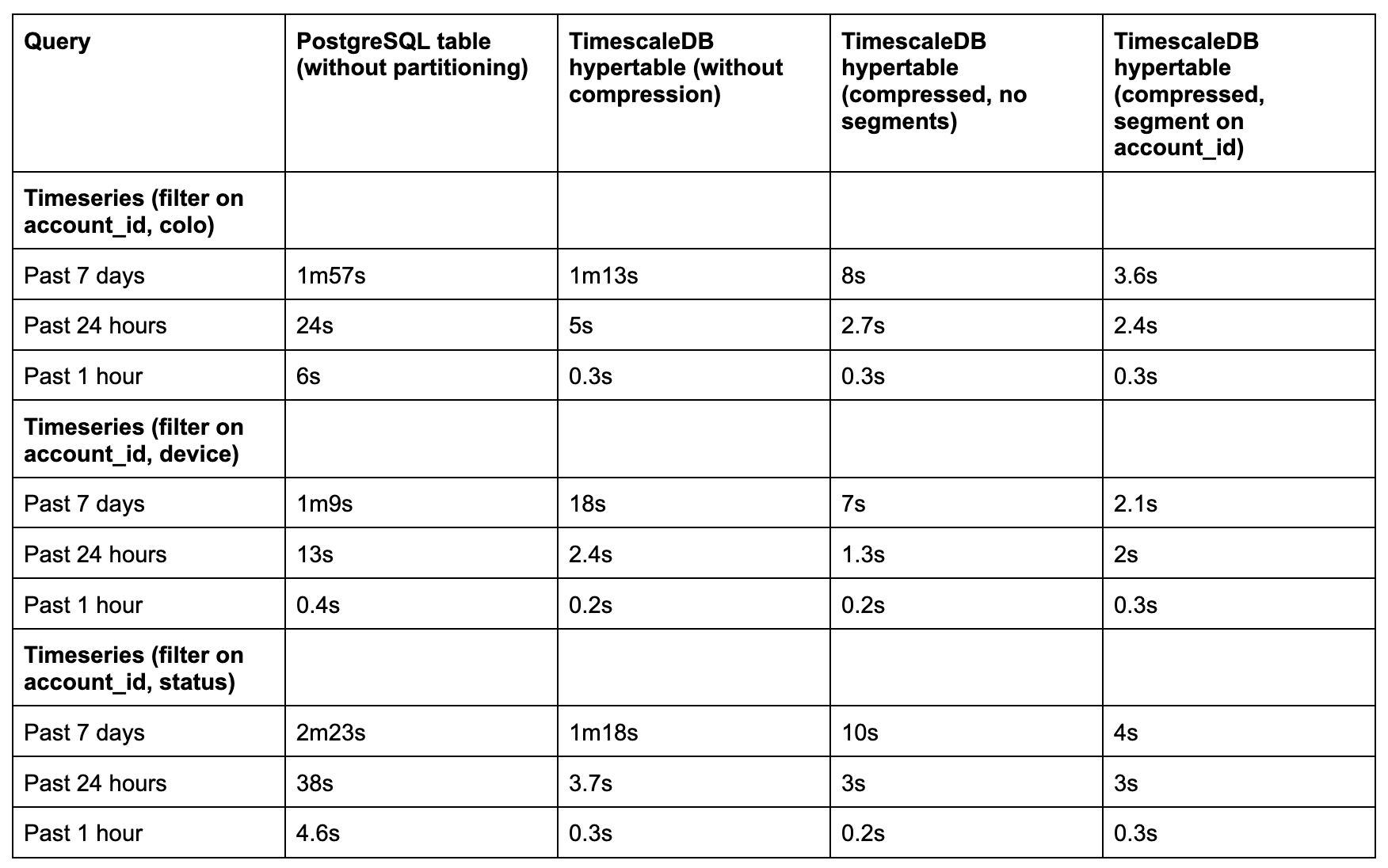
After a two-week backfill period, we ran side-by-side benchmarks using real production queries from our dashboard. We tested:
3 time windows: past 1 hour, 24 hours, and 7 days
3 columnstore modes: uncompressed, compressed, and compressed with segmenting
Datasets containing 500 million to 1 billion rows
We saw 5x to 35x performance improvements, depending on query type and time range:
For short windows (1–24 hours), even uncompressed hypertables performed well.
For longer windows (7 days), compression and columnstore settings (especially with segmentby) made all the difference.
Sparse indexes were critical. Once PostgreSQL’s btree indexes broke down at scale, Timescale’s minmax sparse indexes and columnar layout outperformed.
On top of query performance, we saw impressive compression ratios, up to 33x:
SELECT
    pg_size_pretty(before_compression_total_bytes) as before,
    pg_size_pretty(after_compression_total_bytes) as after,
    ROUND(before_compression_total_bytes / after_compression_total_bytes::numeric, 2) as compression_ratio
FROM hypertable_compression_stats('device_state');

before: 1616 GB
after: 49 GB
compression_ratio: 32.83
That meant we could retain 33x more data for the same cost.
What makes columnstore so fast?
Two main things: compression and sparse indexes.
It might seem counterintuitive that querying compressed data, which requires decompression, can be faster than querying raw data. But in practice, input/output (I/O) is the major bottleneck in most analytical workloads. The reduction in disk I/O from compression often outweighs the CPU cost of decompressing. In TimescaleDB, compression transforms a hypertable into a columnar format: values from each column are grouped in chunks (typically 1,000 at a time), stored in arrays, and then compressed into binary form. More detailed explanation in this TimescaleDB blog post.
You might wonder how this is possible in PostgreSQL, which is traditionally row-based. TimescaleDB has a really clever solution for it by utilizing PostgreSQL TOAST pages. The way it works is after tuples of 1000 values are compressed, they’re moved to external TOAST pages. The columnstore table itself then basically becomes a table of pointers to TOAST, where actual data is stored and only retrieved lazily, column-by-column.
The second factor is sparse minmax indexes. The idea behind sparse indexes is that rather than storing every single value in an index, store every N-th value. This makes them much smaller and more efficient to query in very large datasets. TimescaleDB implements minmax sparse indexes, where for each compressed tuple of 1,000 values it creates two additional metadata columns, storing min and max values. The query engine then looks at these columns to determine whether a value could possibly be found in a compressed tuple before attempting to decompress it.
What we found later, unfortunately, after we did our evaluation of TimescaleDB, is that sparse indexes need to be explicitly enabled via timescaledb.orderby option. Otherwise, TimescaleDB sets it to some default value, which may not always be the most efficient for your queries. We added all columns that we filter on to orderby setting:
– Add columnstore settings
ALTER TABLE device_state SET (
    timescaledb.enable_columnstore,
    timescaledb.segmentby = ‘account_id’,
    timescaledb.orderby = ‘timestamp,device_id,colo,mode,status,client_version,client_platform
);
TimescaleDB at Cloudflare
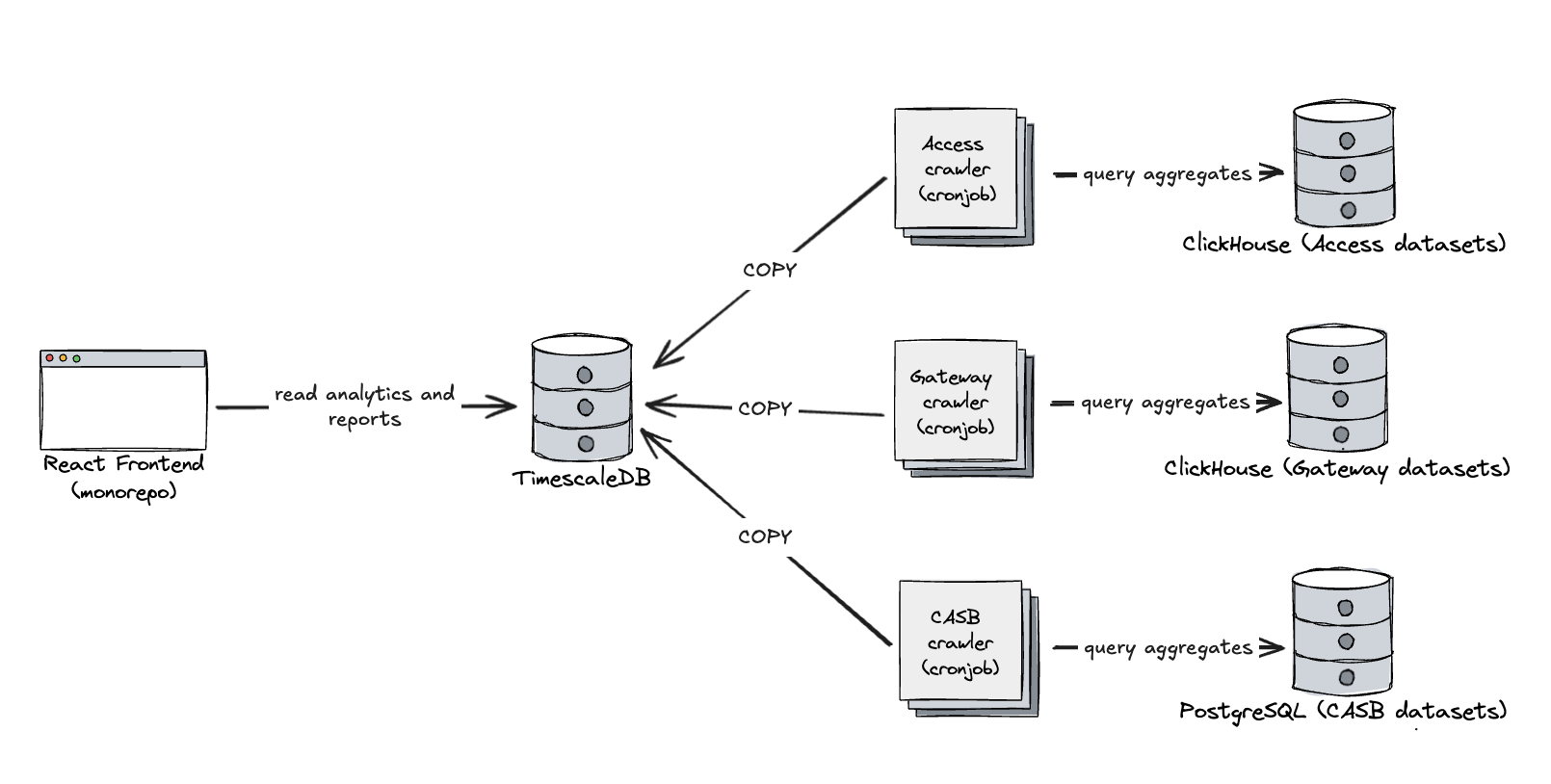
Following the success with DEX, other teams started exploring TimescaleDB for its simplicity and performance. One notable example is the Zero Trust Analytics & Reporting (ART) team.
The ART team is responsible for generating analytics and long-term reports — spanning months or even years — for Zero Trust products such as Access, Gateway, CASB, and DLP. These datasets live in various ClickHouse and PostgreSQL clusters that we wanted to replicate into a singular home that is specifically designed to unify related, but not co-located data points, together and modeled to address our customer’s analytical needs.
We chose to use TimescaleDB as the aggregation layer on top of raw logs stored elsewhere. We built a system of crawlers using cron jobs that periodically query the multitude of clusters for hourly aggregates across all customers. These aggregates are ingested into TimescaleDB, where we use continuous aggregates to further roll them up into daily and monthly summaries for reporting.
Access and Gateway datasets are massive, often ingesting millions of rows per second. To support arbitrary filters in reporting, crawler queries group by all relevant fields, including high-cardinality columns like IP addresses. This means the downsampling ratio is low, and in some cases, we’re inserting ~100,000 aggregated rows per second. TimescaleDB handles this load just fine, but to support it we made some adjustments:
We switched from bulk INSERTS to COPY. This significantly improved ingestion throughput. We didn’t benchmark it ourselves, but plenty of benchmarks show that COPY performs much better with large batches.
We disabled synchronous replication. In our case, temporary data loss is acceptable — our crawlers are idempotent and can reprocess missing data as needed.
We also disabled fsync. Again, durability is less of a concern for this use case, so skipping disk syncs helped with ingest performance.
We dropped most indexes in hypertables, only kept one on (account_id, timestamp), and relied on aggressive compression and sparse indexes. The absence of indexes helped with insert rates and didn’t have a significant impact on query performance, because only a very small part of the table was uncompressed and relied on traditional btree indexes.
Prioritizing core value and resisting the urge to prematurely optimize can accelerate time to market—and sometimes take you on an unexpected journey that leads to better solutions than you’d originally planned. In the early days of DEX, taking a step back to focus on what truly mattered helped us discover TimescaleDB, which turned out to be exactly what we needed.
Not every team needs a hyper-specialized race car that requires 100 octane fuel, carbon ceramic brakes, and ultra-performance race tires: while each one of these elements boost performance, there’s a real cost towards having those items in the form of maintenance and uniqueness. For many teams at Cloudflare, TimescaleDB strikes a phenomenal balance between the simplicity of storing your analytical data under the same roof as your configuration data, while also gaining much of the impressive performance of a specialized OLAP system.
Check out TimescaleDB in action by using our robust analytics, reporting, and digital experience monitoring capabilities on our Zero Trust platform. To learn more, reach out to your account team or sign up directly here.
We think computing or computer science (CS) needs to be accessible to all learners, and we know that teachers work hard towards this. Traditional CS approaches can lack flexibility, creating barriers to learning and excluding some young people. In today’s blog, we’re highlighting the ‘Universal design for learning’ (UDL) framework and how you can use it to make computing education more accessible to all your learners.
Find practical tips for how to use the UDL framework and related approaches with your learners
Read a summary of the research behind the framework
Universal Design for Learning: Because one size does not fit all
Everyone is different and has their own way of learning. What works for one young person may not work for the next. So why should we expect learners to be taught the same material in the same way?
Todd Rose, a contributor to the UDL framework, highlights the factors involved with a young person’s ability to engage and participate in learning. These include cognitive, social-emotional, family background and academic factors. He dispels the idea of an “average” learner, and instead suggests the concept of learner variability.
The new Quick Read
As educators, it’s important to consider that students will likely be at different stages of understanding, and a one-size-fits-all approach isn’t suitable. The UDL framework avoids this mindset and provides teachers with structured guidelines to design accessible lessons from the beginning.
What is the UDL framework?
The UDL framework encourages educators to provide flexibility for learners in three areas:
Multiple means of engagement: The “why of learning”, which helps to pique students’ curiosity and motivates them to stay engaged
Multiple means of representation: The “what of learning”, which focuses on presenting information in different ways to make the content accessible
Multiple means of action and expression: The “how of learning”, which relates to different ways for students to access learning and express their understanding
How can I apply the UDL framework?
Two things are key while you are planning how to apply the UDL framework with your learners:
Try not to introduce all three areas at once to your practice. Instead, focus on one area of the framework at a time and reflect to identify where there might be gaps. Focus on these first and make changes one by one.
Consider how different approaches will work for different groups and individuals. Try to identify what works for your learners and vary or adapt your approach as necessary.
Applying UDL: Some ideas for teaching programming
Multiple means of engagement — show learners different reasons for engaging in programming. For example:
Solving real-life problems
Interest in technology or logical thinking
Creative expression
Multiple means of representation — teach programming concepts in multiple ways. For example:
Demonstrate through live coding
Write on a blackboard with a flowchart
Let learners label and assemble bits of paper into a ‘program’
Multiple means of action and expression — teach with accessibility in mind. For example:
Use tools appropriate for learners’ mouse and keyboard skills
Let learners demonstrate their understanding in different ways (e.g. verbally, by writing/drawing, by creating a program)
The UDL framework aligns closely with several key research-supported pedagogies that you can use for effective instruction in computational thinking and programming. For example, the pedagogy approach ‘Use-Modify-Create’ (UMC) can be paired with the UDL categories. The new Quick Read explores these connections in more detail.
The benefits of the UDL framework
Potential benefits for teachers:
The framework provides a clear structure for designing learning activities that appeal to and engage the widest set of learners
It can help you consider all the ways you might engage your learners and make CS lessons more accessible.
UDL encourages you to reflect on the different ways in which you might represent concepts and ideas
It can help you to build learner agency and independence in your students by offering them different ways to express their learning in CS topics.
Potential benefits for learners:
The framework promotes a sense of ownership over their learning. Which can boost their motivation and resilience to sticking with difficult challenges.
They will likely find content that resonates with them, leading to higher engagement and therefore learning.
They will be able to demonstrate their CS knowledge confidently and engage limitlessly in CS contexts.
Our new Quick Read shares tips on how to best use the framework in your teaching.
“The reality is that access to the opportunities to learn about computer science, programming, and coding has remained deeply unequal, both within and between countries. That has helped create a technology sector that doesn’t reflect the broad diversity of human backgrounds, perspectives, and experiences. And we are all living with the consequences.” – Philip Colligan, Mark Griffiths, Veronica Cucuiat
“If we don’t have a diverse range of people designing and implementing that tech, then we are going to come across issues.” – Becky Patel, Tech She Can, Hello World podcast”
By embracing the principles of ‘Universal design for learning’ and similar approaches, we can create a more inclusive and equitable learning environment in computer science for everyone.
To provide the best experiences, we use technologies like cookies to store and/or access device information. Consenting to these technologies will allow us to process data such as browsing behavior or unique IDs on this site. Not consenting or withdrawing consent, may adversely affect certain features and functions.
Functional
Always active
The technical storage or access is strictly necessary for the legitimate purpose of enabling the use of a specific service explicitly requested by the subscriber or user, or for the sole purpose of carrying out the transmission of a communication over an electronic communications network.
Preferences
The technical storage or access is necessary for the legitimate purpose of storing preferences that are not requested by the subscriber or user.
Statistics
The technical storage or access that is used exclusively for statistical purposes.The technical storage or access that is used exclusively for anonymous statistical purposes. Without a subpoena, voluntary compliance on the part of your Internet Service Provider, or additional records from a third party, information stored or retrieved for this purpose alone cannot usually be used to identify you.
Marketing
The technical storage or access is required to create user profiles to send advertising, or to track the user on a website or across several websites for similar marketing purposes.


 Neeraj Kaushik is an Open Group Certified Distinguish Architect at IBM with two decades of experience in client-facing delivery roles. His experience spans several industries, including travel and transportation, banking, retail, education, healthcare, and anti-human trafficking. As a trusted advisor, he works directly with the client executive and architects on business strategy to define a technology roadmap. As a hands-on Chief Architect AWS Professional Certified Solution Architect, AWS Certified Machine Learning Specialist and Natural Language Processing Expert, he has led multiple complex cloud modernization programs and AI initiatives.
 Jay Pandya is a Senior Partner Solutions Architect in the Global Systems Integrator (GSI) team at Amazon Web Services (AWS). He has over 30 years of IT experience and is helping and providing guidance to AWS GSI partners to build, design, and architect agile, scalable, highly available, and secure solutions on AWS. Outside of the office, Jay enjoys spending time with his family and traveling, and he is an aviation enthusiast and avid sports and Formula 1 fan.
 Vijay Gokarn is a Senior Solution Architect at IBM with extensive experience across industries including financial services, healthcare, industrial, retail, and travel and hospitality. He leads complex AWS transformation initiatives, drawing on his hands-on expertise as an AWS Certified Solutions Architect Associate. Vijay specializes in serverless architectures, event-driven systems, and enterprise modernization. As a skilled architect and team leader, he has delivered impactful solutions in cloud modernization, digital banking, and intelligent automation. His passion lies in bridging business strategy with technical execution to drive scalable digital transformation.
 Subhash Sharma is Sr. Partner Solutions Architect at AWS. He has more than 25 years of experience in delivering distributed, scalable, highly available, and secured software products using Microservices, AI/ML, the Internet of Things (IoT), and Blockchain using a DevSecOps approach. In his spare time, Subhash likes to spend time with family and friends, hike, walk on beach, and watch TV.