Post Syndicated from xkcd.com original https://xkcd.com/3326/
Post Syndicated from xkcd.com original https://xkcd.com/3326/
Post Syndicated from Dirk Fröhner original https://aws.amazon.com/blogs/big-data/reduce-the-complexity-and-cost-of-real-time-processing-with-queues-in-amazon-kinesis-data-streams/
Teams use Amazon Kinesis Data Streams to ingest data once and make it available to every application that needs to consume it in real time. Some of those applications process related records in sequence, building each result on the records before it. Others process each record independently.
Consider an online store that writes every order event to a stream. One application processes the orders in sequence to catch possible fraud. Its state is a count of each customer’s recent orders. It updates that count with every order and flags any customer who places an unusual number in a short time (stateful processing). The fulfillment application processes each order independently, reserving inventory and starting the shipment. It treats every record as a self-contained unit of work that it can process and retry by itself (stateless processing).
Kinesis Data Streams and the Amazon Kinesis Client Library (KCL) are built for the first job. The KCL assigns each shard to one consumer instance at a time, using a lease table in Amazon DynamoDB. The records for a customer reach the same instance in the order they were written. The application saves its progress as a checkpoint, a position in the shard, so after a restart it resumes from where it left off instead of starting over. Applications that read the stream directly this way are called stream consumers in this post. For the fraud check described earlier, each of these mechanics is what keeps its counts accurate.
The fulfillment application doesn’t need orders in sequence, but because it reads shards, it still gets one consumer instance per shard. An on-demand stream sizes its shards for throughput, not for processing time. With 10 shards, at most 10 instances process orders, no matter how far the application falls behind. A checkpoint is a single position in the shard, so the application can’t mark one order as failed and the next one as done. Teams build that per-record tracking, retries, and failure handling themselves. An order that keeps failing either holds up every order behind it in the shard or is skipped, unless their code sets it aside. They still run the lease table and per-shard custom metrics in Amazon CloudWatch to coordinate and monitor their instances. Other teams copy the records into an Amazon Simple Queue Service (Amazon SQS) queue to get per-record tracking without building it. This means ingesting the same data twice and running a relay in between.
Today, AWS introduced queues in Amazon Kinesis Data Streams. A queue delivers the records of an on-demand data stream to your application and tracks the delivery state of each record. The application acknowledges each record when it’s done instead of checkpointing a position. Consumer instances don’t lease shards, so you add instances to process more records in parallel. The queue redelivers any record that isn’t acknowledged in time, and sets aside records that keep failing as dead-letter records. A record that repeatedly fails stops wasting consumer resources and can be inspected and triaged separately. Because the queue does this tracking and publishes its own metrics, your consumer no longer needs a lease table or per-shard custom metrics. This also lowers what it costs to run. You ingest your data once, and the same stream feeds stream consumers, queues, and managed delivery to streaming tables or Amazon Simple Storage Service (Amazon S3) for batch processing. There’s no relay or second copy of the data. Figure 1 illustrates these three consumption and delivery options.
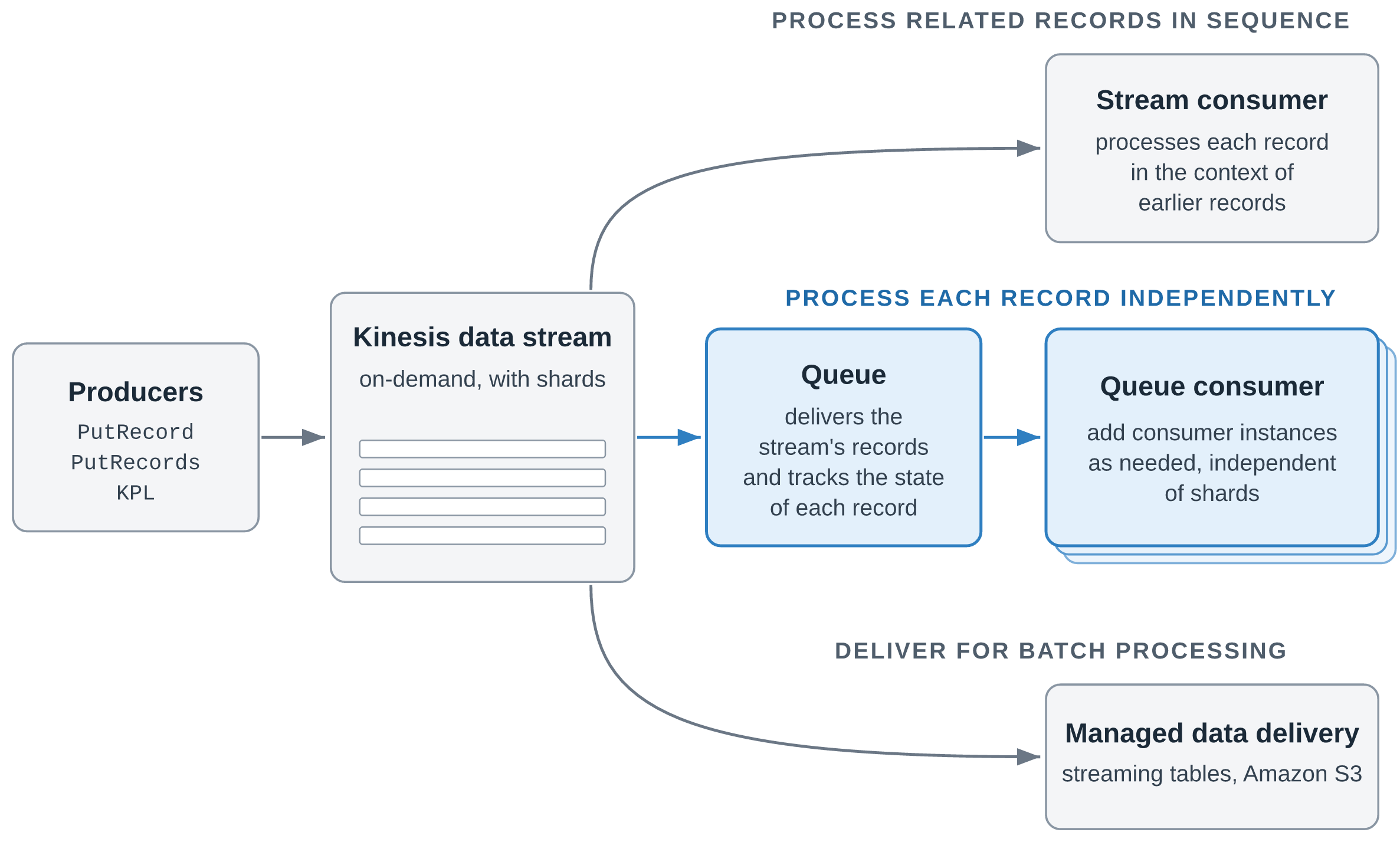
Figure 1: One stream, three ways to consume and deliver its records
Receiving records through a queue is priced at the same rate as data retrieval from the stream. The cost difference comes from the DynamoDB and CloudWatch charges you no longer pay and from compute you use more efficiently. Each consumer instance can run as many parallel threads as it needs to use its CPU fully. Kinesis Data Streams consumers can reduce the cost of processing data by up to 43 percent by using queues instead of the Kinesis Client Library. Actual savings depend on your workload and configuration.
In this post, we walk through how queues work, explain when to use a queue and when to read the stream directly, show where the saving comes from and how AWS measured it, and introduce a sample repository with working code for the main scenarios.
A queue is a Kinesis resource that you create for an existing on-demand stream with CreateQueue. Your consumer application, called a queue consumer in this post, then reads records from the queue instead of from shards. Each running copy of the application is a consumer instance. A queue consumer works in three steps:
ReceiveQueueRecords and gets a batch of up to 10 records. Each record it receives is hidden from other consumer instances for a period called the visibility timeout, so two consumer instances don’t process the same record at the same time.AcknowledgeQueueRecords, and the queue doesn’t deliver the record again. If the consumer instance fails before it acknowledges, the visibility timeout expires and any consumer instance can receive the record again.Consumer instances compete for records: each receives the next available records, so you add instances when the backlog grows. Delivery is at least once, and ordering is best effort.
You can create several queues for a stream, one for each consuming application. Queues count toward the stream’s limit on registered consumers, which they share with enhanced fan-out consumers: 50 for an On-demand Advantage stream and 20 for an On-demand Standard stream. A queue’s receive throughput is virtually unlimited, and adding a queue doesn’t change anything for your producers or your existing stream consumers. Each queue also tracks its own delivery state: acknowledging a record in one queue doesn’t affect other queues or the record in the stream.
When you create a queue, you choose where in the stream it starts delivering records:
| Starting position | The queue delivers |
LATEST (default) |
Records that arrive after the queue is created |
TRIM_HORIZON |
All records still in the stream, starting with the oldest |
AT_TIMESTAMP |
Records from a point in time that you choose |
With TRIM_HORIZON or AT_TIMESTAMP, a new application starts with data that’s already in the stream.
Figure 2 shows the states of a record in a queue and the operations that move it between them.
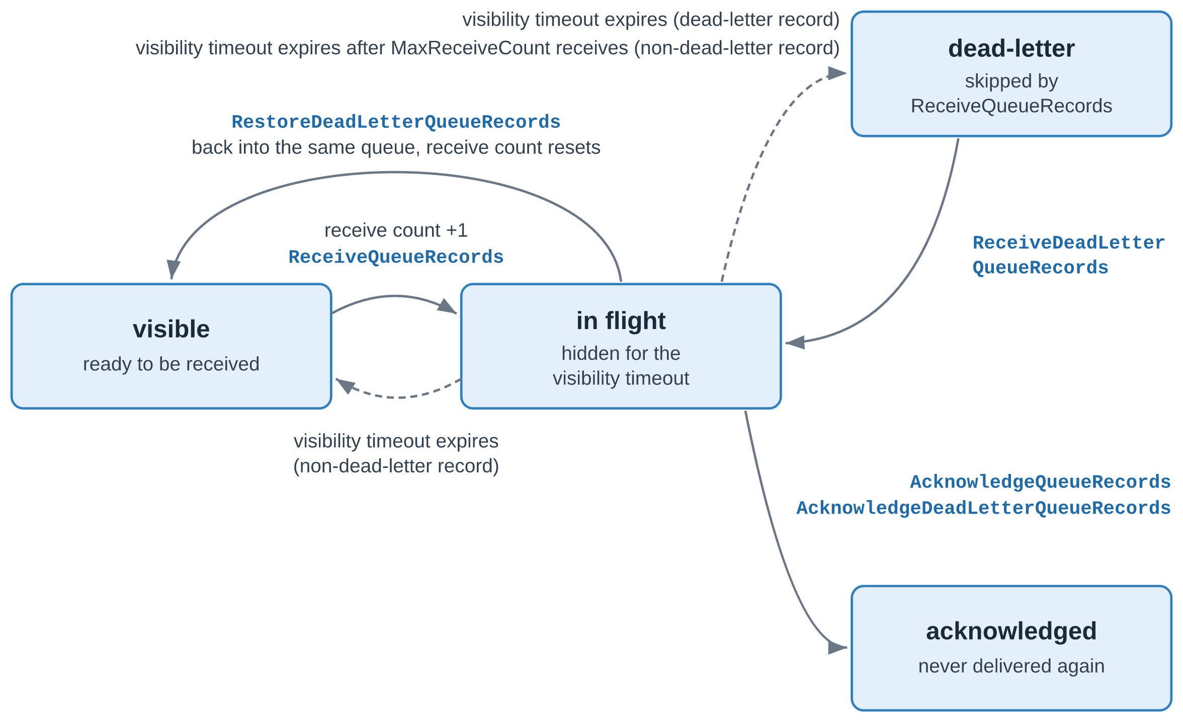
Figure 2: The lifecycle of a record in a queue
A record that a consumer instance receives is in flight and hidden from other consumer instances until its visibility timeout expires. The timeout defaults to 30 seconds and can be set up to 12 hours. A consumer instance can extend it with UpdateQueueRecordsVisibility, or set it to 0 to release the record immediately. If the timeout expires before an acknowledgment, the record becomes visible again and its receive count goes up by one.
A record can keep failing because of its content, for example a malformed payload or an order for a product that no longer exists. It can also fail because of a problem on your side, such as an unavailable downstream service or a bug in your consumer. Dead-letter handling, enabled by default, moves a record to the dead-letter state after MaxReceiveCount receives without an acknowledgment (six by default), so that it stops taking capacity from your consumer instances. You can change the count or disable dead-letter handling with CreateQueue or UpdateQueue, or by using the console. With dead-letter handling disabled, failing records keep returning until their retention period in the stream ends.
You work with dead-letter records through a separate set of operations: ReceiveDeadLetterQueueRecords to receive them, RestoreDeadLetterQueueRecords to return them to the normal receive path with a reset receive count, and AcknowledgeDeadLetterQueueRecords to discard them. These operations have their own AWS Identity and Access Management (IAM) actions, so an operator role can handle dead-letter records without changing your consumer’s permissions. The queue also publishes dead-letter metrics such as VisibleDeadLetterQueueRecords, so you can alarm on them. Acknowledge records that can never succeed to discard them. For records that failed because of a broken dependency or a consumer bug, fix the cause first, then restore them. Like any other record, a dead-letter record expires when its retention period in the stream ends.
A consumer instance can receive a record more than once: after a visibility timeout expires, after a restore, or on rare occasions even after an acknowledgment. Because delivery is at least once, make your processing idempotent. Each record carries a RecordId that stays the same across redeliveries and across queues on the stream. A producer retry, however, writes the same data to the stream a second time, and the duplicate arrives as a new record with a different RecordId. Key your side effects on a business ID, such as the order ID, for example with a conditional write. Where records carry no business ID or you don’t control the producers, fall back to RecordId. Size the visibility timeout to your processing time, and extend it for the occasional long-running record. AcknowledgeQueueRecords returns HTTP 200 with separate Successful and Failed lists, so check the Failed list on every call.
Each queue publishes its own metrics to CloudWatch, including VisibleQueueRecords for records ready to be received, InFlightQueueRecords for records that are received but not yet acknowledged, and matching metrics for dead-letter records. Scale your consumer instances on VisibleQueueRecords, and alarm on VisibleDeadLetterQueueRecords so that you notice failing records early.
With the addition of queues, Kinesis Data Streams now offers two ways to process a stream’s records in real time, and each application can use the one that fits its work:
The following table compares the two:
| Stream consumer | Queue consumer | |
| Typical work | Aggregations, windowed analytics, fraud and anomaly detection | Order fulfillment, per-record inference, record enrichment, search indexing |
| Ordering | In order for each partition key | Best effort |
| Parallelism | Each shard is read by one sticky consumer instance of an application at a time | Add consumer instances as needed, independently of the shard count |
| Progress tracking | The application stores its read position, for example in the KCL lease table | The queue tracks the delivery state of every record |
| Failed records | Retried in place, which holds up the shard, or skipped and tracked by your code | Redelivered individually, then set aside as dead-letter records |
| Tooling | KCL, Amazon Managed Service for Apache Flink | AWS SDK |
Besides the DynamoDB and CloudWatch charges, the saving comes from compute. A KCL consumer instance processes each shard’s records one batch after another, so with I/O-bound processing it spends much of its time waiting. The load also depends on partition keys: if most records share one partition key, that shard is processed in sequence while the instances that lease other shards sit idle. A queue consumer instance can run as many parallel threads as it needs to use its CPU fully, so fewer instances handle the same throughput.
An AWS benchmark measured the saving with a synthetic workload, not a real-world customer workload, for which AWS specified the record size, rate, partition-key distribution, and handler cost. A KCL 3.5.3 fleet and a queue fleet consumed the same On-demand Advantage stream at the same time, at a sustained throughput of 25 MB/s with a warm throughput of 100 MB/s. Each fleet was sized to process 99 percent of records within 10 seconds. The comparison covers data retrieval or queue consumption, DynamoDB, CloudWatch, and Amazon Elastic Compute Cloud (Amazon EC2) at US East (Ohio) prices. It excludes ingestion, which costs the same for both. The benchmark tested one handler profile, with 1 ms of CPU and 10 ms of wait per record. This I/O-bound profile is the most favorable condition for the compute part of the saving, and a CPU-bound handler narrows it. Of the $15.09 saving per TiB, $11.55 comes from DynamoDB and CloudWatch, which don’t depend on the handler. Even with no compute advantage, the saving would still be 33 percent. The KCL fleet ran with its default configuration, including detailed metrics with the shard dimension, which produced 1,580 metric series at 190 shards. If you reduce KCL metrics to the summary level without the shard dimension, this part of the saving shrinks, at the cost of per-shard observability.
Queues in Kinesis Data Streams are powered by Amazon SQS. Built on that foundation, they use familiar queue concepts such as visibility timeouts, acknowledgments, and dead-letter handling. They’re a capability of Kinesis Data Streams, and you work with them through the Kinesis Data Streams APIs.
Amazon SQS continues to be the place to start for point-to-point messaging between application components, such as buffering requests, decoupling services, and background jobs, where no other application needs the same data.
Choose queues in Kinesis Data Streams when the same records are needed by more than one application. There’s no dual ingest and no relay to operate. Applications that process each record independently receive and acknowledge each record through the AWS SDK, with no KCL, lease table, or shards to manage.
The GitHub repo contains working code for six scenarios, written in TypeScript, with Java for the KCL consumers, and deployed with the AWS Cloud Development Kit (AWS CDK). Each scenario builds on a quickstart with an on-demand stream, an order producer, and a KCL consumer on AWS Fargate, and the README lists the prerequisites and the cleanup steps. The scenarios are the following:
AT_TIMESTAMP.In the KCL migration, a receive and acknowledge loop replaces the KCL, its lease table, and custom metrics, and the processing logic stays. When the SQS queue behind a relay carries only records from the stream, a queue in Kinesis Data Streams replaces both the relay and the SQS queue. If other applications also send messages to that SQS queue, keep it. The consumer’s API calls map as follows:
| Amazon SQS | Kinesis queue |
ReceiveMessage |
ReceiveQueueRecords |
DeleteMessage, DeleteMessageBatch |
AcknowledgeQueueRecords |
ChangeMessageVisibility, ChangeMessageVisibilityBatch |
UpdateQueueRecordsVisibility |
| Dead-letter queue with a redrive policy | Dead-letter state in the same queue, restored with RestoreDeadLetterQueueRecords |
Both migrations pick a starting position that skips no records, and tolerate duplicates while old and new consumers overlap.
Queues in Kinesis Data Streams are built for work where each record stands on its own. They scale with your backlog instead of your shard count, track every record for you, and set failing records aside so that they don’t hold up the rest. Stream consumers remain the right choice for work that depends on the order of records. Kinesis queues are powered by Amazon SQS and use familiar queue concepts such as visibility timeouts, acknowledgments, and dead-letter handling. You ingest your data once, and stream consumers, queues, and delivery to Amazon S3 all read from the same stream. If you run stateless KCL consumers, moving them to a queue can also lower your processing cost.
For Regional availability, see Supported AWS Regions. For pricing, see Amazon Kinesis Data Streams pricing. To get started, create a queue for an on-demand stream on the Kinesis console or with CreateQueue, and run the scenarios in the GitHub repo. For more information, refer to Consume records from a stream with queues in the Amazon Kinesis Data Streams Developer Guide. For help with your use case, contact your AWS representative.
Post Syndicated from Pengfei Shao original https://aws.amazon.com/blogs/security/introducing-simplified-onboarding-for-aws-waf-bot-control-at-the-targeted-inspection-level/
Today, we’re announcing simplified onboarding and bot confidence levels for AWS WAF Bot Control at the targeted inspection level, which we refer to as Targeted bot control in this post, matching the console. Bot confidence levels and the new LATEST rule group version are available for the resource types that AWS WAF protects: you act on advanced bot detections by confidence level instead of writing label rules, and you stay on the newest detections without manual upgrades, helping you respond to automated traffic, including traffic from AI-powered bots. For the websites and applications that you deliver through Amazon CloudFront, simplified onboarding goes further: you turn on Targeted bot control from a single console setting, and automatic SDK integration, which launched last month, removes the need for application code changes in many cases.
In this post, we explain what the simplified onboarding experience looks like and how to get started when protecting CloudFront-delivered applications.
Targeted bot control uses advanced behavioral analysis designed to help identify sophisticated bots that attempt to evade traditional detection mechanisms. It uses machine learning and client-side signals to help detect sophisticated AI-based bots. It’s also deliberately granular: it surfaces each detection as its own label, so you can build rules around specific behaviors. The number of choices (which labels, which combinations, and which order) is a lot to evaluate and implement when your immediate goal is to implement the first round of protections.
To get the full value of Targeted bot control, and to help reduce false positives by grouping its signals into confidence levels, you typically do the following:
We’ve published guidance on grouping targeted bot labels into confidence tiers. For teams without dedicated security engineers, the path to implement the solution can be long. Completing every step can take time, especially when the SDK integration depends on another team’s release cycle, so rules can remain in Count mode longer than intended.
You can now turn on Targeted bot control with a single toggle. AWS WAF sets up the recommended configuration for you and keeps it on the latest detections, and you don’t need to change your application code to integrate AWS WAF JavaScript SDK for CloudFront-delivered applications in many cases. When you use this toggle, AWS WAF configures the following for you:
LATEST version, which points to the most recent AWS WAF Bot Control release, so you get new detections without upgrading manually.With bot confidence, AWS WAF Bot Control now adds a High, Medium, or Low bot confidence level to each request that it evaluates at the targeted inspection level. The confidence level reflects how likely it is that the request comes from an automated client that exhibits behaviors that you might not want.
Several AWS WAF Bot Control rules already report their own confidence levels with AWS WAF labels, for example TGT_ML_CoordinatedActivityLow/Medium/High and TGT_TokenReuseIpLow/Medium/High rules, and the TGT_VolumetricSession rule emits labels ending in volumetric:session:low, volumetric:session:medium, and volumetric:session:high. Each of those describes the strength of one detection. Bot confidence combines the targeted detections into one High, Medium, or Low level for each request, so you choose one action per level instead of writing rules across many labels. Bot confidence also emits three labels ending in targeted:signal:bot_signal:low, targeted:signal:bot_signal:medium and targeted:signal:bot_signal:high.
The confidence levels and their default actions reflect AWS recommendations to AWS WAF Bot Control customers.
| Confidence level | What it indicates | Default action |
|---|---|---|
| High | A signal that by itself strongly indicates automation, or two or more signals that corroborate each other | CAPTCHA |
| Medium | A signal that indicates automation, but no other signal corroborates it; the request might still come from a person | CAPTCHA |
| Low | Only weak signals of automation | Challenge |
The defaults are chosen to help keep false positives low. High-confidence and Medium-confidence bot traffic receives a CAPTCHA puzzle rather than a block, so a misclassified user can still get through. Low-confidence bot traffic receives a silent Challenge, which is designed to complete in the browser without requiring user interaction. You can change any of these actions to Allow, Block, CAPTCHA, Challenge, Count, or Monetize.
The confidence levels are added alongside the existing AWS WAF Bot Control labels. The existing detection labels that AWS WAF Bot Control emits are still attached to the request, so you can inspect any request and see which signals contributed to its confidence level.
The AWS WAF JavaScript SDK runs in the viewer’s browser, where it can see signals the server doesn’t normally receive, such as mouse movements, key presses, form interactions, and device characteristics. These client-side signals help improve the accuracy of the targeted detections in distinguishing between a person and an automated client. The SDK silently acquires and refreshes an AWS WAF token as the page loads, without the extra charges or interruptions of Challenge and CAPTCHA rule actions.
That token travels with each request and is used by AWS WAF Bot Control at the targeted inspection level, AWS WAF Fraud Control account takeover prevention, and AWS WAF Fraud Control account creation fraud prevention. Until now, integrating the SDK meant adding a script tag to your pages yourself.
With automatic SDK integration for CloudFront, you don’t add the script tag yourself. When the setting is on, CloudFront inserts the same script tag that a manual integration uses, pointing to your protection pack’s integration URL. AWS WAF evaluation, token acquisition, and token refresh work the same way as they do with a manual integration.
Automatic SDK integration is available for any protection pack with the CloudFront scope that contains one of the following managed rule groups:
For the up-to-date list of managed rule groups supporting this feature, see Automatic SDK integration for CloudFront distributions.
A rule group also qualifies when its actions are overridden to Count, so you can add the SDK while you evaluate the rule group. When you create a new protection pack with the CloudFront scope in the console, automatic SDK integration is turned on by default. Protection packs created before the feature launched aren’t changed. You can also turn the setting off with a single toggle if you prefer to integrate the SDK yourself. The SDK collects client-side signals and stores the AWS WAF token in a cookie named aws-waf-token. The token contains information collected from your visitors’ browsers. As described in AWS WAF token characteristics, the information gathered is non-unique and can’t be mapped to an individual human being. Before you turn on automatic SDK integration, review your privacy notice and any cookie consent obligations that apply to your sites, for example under GDPR and the ePrivacy Directive.
In this section, we show you how to enable Targeted bot control with bot confidence and automatic SDK integration for CloudFront.
To follow this walkthrough, you need the following:
When you create a new protection pack, you can turn on Targeted bot control together with automatic SDK integration.
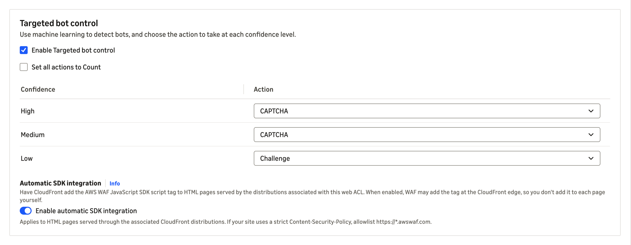
Figure 1: The Targeted bot control section during protection pack creation
These steps work whether your protection pack doesn’t yet have AWS WAF Bot Control, uses AWS WAF Bot Control at the common level, or uses an older AWS WAF Bot Control version.
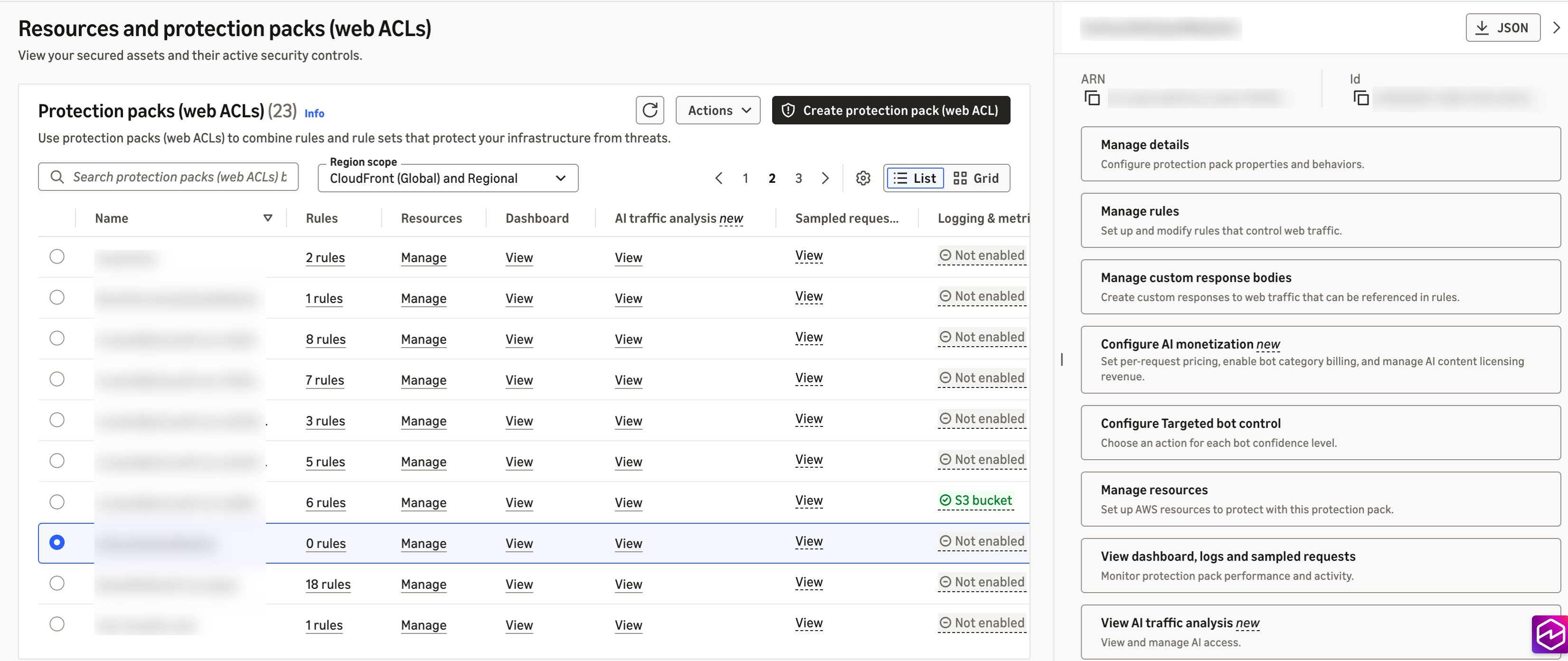
Figure 2: Choosing an existing protection pack
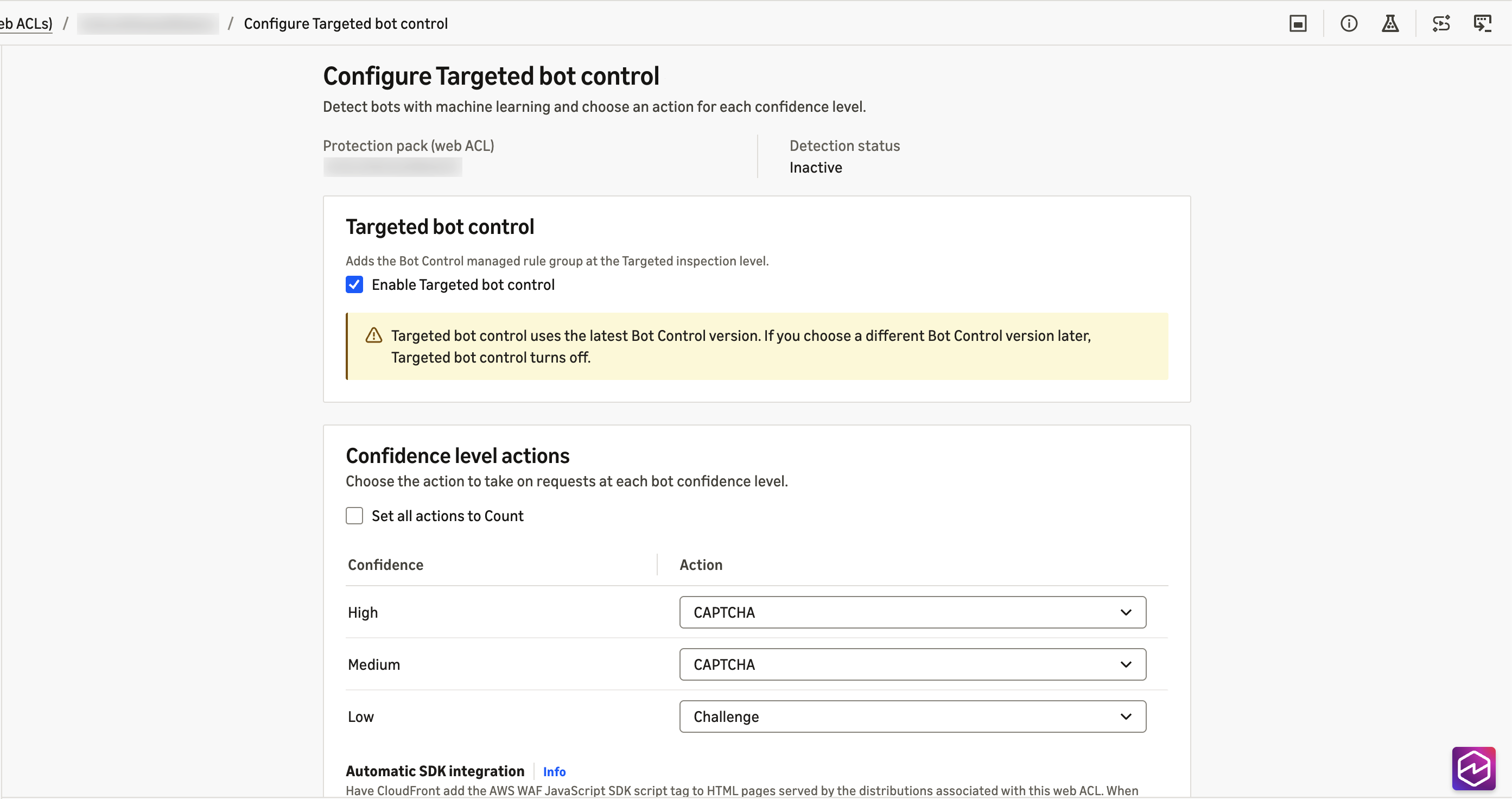
Figure 3: The Configure Targeted bot control page
LATEST, a confirmation dialog shows the current and target versions. Review it and confirm.If you manage AWS WAF as code, you can configure the same pieces directly. For automatic SDK integration, add the ChallengeJavascriptSdkInjection setting to the AssociationConfig of the web ACL in a CreateWebACL or UpdateWebACL request, using the CLOUDFRONT key with an empty configuration object:
Through the API, the setting is off by default. An UpdateWebACL request that omits the setting turns it off, even if you turned it on in the console. For the rule group, set the inspection level to TARGETED with machine learning enabled in the AWSManagedRulesBotControlRuleSet configuration, and use RuleActionOverrides to set the actions for TGT_SignalBotHigh, TGT_SignalBotMedium, and TGT_SignalBotLow.
For the API specifications, see AssociationConfig and ManagedRuleGroupStatement in the AWS WAF API Reference.
Considerations when using bot confidence and automatic SDK integration for CloudFront:
Review the following when you use bot confidence.
LATEST version. Bot confidence requires version 8.0 or later. LATEST keeps you on the newest release automatically; if you pin a static version for change control, choose 8.0 or later and review new versions as they’re released.For the full list of considerations about bot confidence, see Bot confidence levels in the AWS WAF Developer Guide.
Review the following before you turn on automatic SDK integration.
https://*.awswaf.com in the directives shown in Using the JavaScript API with content security policies.Cache-Control: no-transform to keep the tag off specific pages. The setting applies to the whole protection pack, and scope-down statements don’t limit where the tag is inserted.For the full list of considerations and edge cases, see Considerations and limitations and When pages don’t receive the tag in the AWS WAF Developer Guide.
Simplified onboarding to Targeted bot control is available for protection packs with the CloudFront scope. Bot confidence levels and the new LATEST rule group version are available for the resource types that AWS WAF protects, in the AWS Regions where AWS WAF Bot Control is available. Automatic SDK integration is available for protection packs with the CloudFront scope. This post focuses on CloudFront because you get both features there.
Standard AWS WAF Bot Control charges for the targeted inspection level apply. Automatic SDK integration for CloudFront is available at no additional cost. For details, see AWS WAF pricing.
Simplified onboarding for Targeted bot control takes care of most of the configuration work. You enable Targeted bot control and choose one action for each of three bot confidence levels, or keep the defaults, and enable automatic SDK integration for CloudFront. Your protection pack starts with the configuration we recommend, stays on the latest detections, and doesn’t require you to integrate the JavaScript SDK manually with your CloudFront-delivered applications.
If you have questions about this post, contact AWS Support or start a new thread on AWS re:Post.
Post Syndicated from Chetan Suri original https://aws.amazon.com/blogs/devops/reducing-database-incident-mttr-by-73-with-a-custom-aws-devops-agent-skill/
Database incidents are among the most time-consuming operational events for Site Reliability Engineering (SRE) teams. When an Amazon Aurora PostgreSQL cluster experiences performance degradation, SRE engineers must correlate metrics across connection pools, replication topology, query performance, storage subsystems, and parameter configurations. These troubleshooting steps routinely take 45–60 minutes even for experienced engineers.
AWS DevOps Agent is an operations teammate that resolves and proactively helps prevent incidents, and optimizes application reliability and performance. It also handles on-demand SRE tasks across AWS, multicloud, and on-premises environments. Although its built-in capabilities handle common scenarios well, most organizations have unique database configurations, connection pooling patterns, and performance baselines. That knowledge lives in the heads of senior database reliability engineers (DBREs).
With Custom Skills, you can codify that expertise and make it available to the agent 24/7. In this post, we walk through building a custom Aurora PostgreSQL performance degradation investigation Skill. This multi-fault procedural Skill uses decision-tree logic that covers five distinct failure modes. We then show how it reduces Mean Time to Resolution (MTTR) from a baseline of 52 minutes to 14 minutes. That’s a 73 percent reduction, measured in a controlled internal test of three simulated incidents.
Before getting started, make sure you have:
DatabaseConnections, ReplicaLag, db.load).Consider a typical Aurora PostgreSQL performance degradation incident. The on-call engineer receives a page indicating elevated read latency. From here, the investigation branches into multiple possible root causes:
Each branch requires checking different metrics, correlating with different timelines, and applying different remediation strategies. A senior DBRE knows which branch to explore first based on subtle signal combinations. However, that knowledge is rarely documented in a way that’s actionable at 2 AM.
Additionally, parameter drift is particularly insidious because its symptoms mimic other failure modes. It occurs when someone modifies the cluster parameter group and introduces a misconfiguration. Without domain-specific guidance, the agent chases symptoms rather than tracing back to the configuration change.
Rather than building five separate Skills (one per failure mode), we build a single procedural Skill with decision-tree logic that mirrors how an expert DBRE triages Aurora PostgreSQL issues. The Skill evaluates initial signals to determine which investigation branch to follow, then executes a structured procedure for that specific failure mode.
The AWS DevOps Agent workshop covers two Skill types: (1) a single-file UI-created checklist (AWS Lambda cold starts) and (2) a multi-file architecture-context Skill (EKS Retail Store). Both are effective for their scope, but neither demonstrates a procedural investigation Skill with decision-tree logic that proves measurable MTTR reduction.
Our Skill differs in three key ways:
Skills are modular instruction sets. Each is a self-contained directory of Markdown files that provides specialized domain knowledge and investigation methodologies to AWS DevOps Agent. Each Skill contains:
The agent evaluates a Skill’s description field in the frontmatter to determine relevance, then loads and follows the instructions during investigations. Skills follow the open Agent Skills specification (agentskills.io), supporting non-executable documents: Markdown, PDFs, images, and data files.
The following steps walk through building the Skill end to end, from documenting the investigation pattern to deploying it. We start by capturing how an expert triages the incident.
Before writing any Markdown, we interviewed three senior DBREs and documented their mental model for Aurora PostgreSQL performance triage. The common pattern:
The SKILL.md begins with frontmatter that tells the agent when to activate, followed by initial signal classification that routes to the correct branch:
| Primary Signal | Likely Branch | Go To |
DatabaseConnections near max or connection errors |
Connection Pool Exhaustion | Branch A |
ReplicaLag > 20 ms or stale read complaints |
Replication Lag | Branch B |
Latency spike with high db.load in Performance Insights |
Slow Query Regression | Branch C |
FreeLocalStorage declining or VolumeBytesUsed alert |
Storage Pressure | Branch D |
| Parameter group change in AWS CloudTrail within past 7 days | Parameter Drift | Branch E |
Critical rule: If multiple signals are present, prioritize A → B → C → D → E. Connection exhaustion masks other symptoms, so it must be checked first.
Investigation procedure. Connection pool exhaustion is the highest-priority branch because it masks every other symptom, so the agent checks it first. It works through four checks in order, moving from the raw connection count to the behavior behind it:
DatabaseConnections against max_connections. If connections exceed 85 percent of the maximum, pool exhaustion is confirmed.idle_in_transaction hold connection slots open and starve the pool.Interpreting the findings. The preceding checks establish what is happening. This is where the agent decides why. Each pattern maps to a distinct root cause:
Investigation procedure. When readers fall behind the writer, the agent needs to know whether the cause is write pressure, reader capacity, or a transient backlog. It gathers four signals before drawing a conclusion:
AuroraReplicaLag for each reader (normal is under 20 ms, critical is over 100 ms).WriteIOPS, WriteThroughput, and WriteLatency to see how hard the writer is working.CPUUtilization and FreeableMemory per reader to spot an overwhelmed instance.db.load with write wait events.Interpreting the findings. The combination of writer pressure and reader health tells the agent which of four situations it is in:
Investigation procedure. A query regression can come from new code, a changed plan, or simply more volume, so the agent compares the current workload against a known-good baseline:
db.load (average active sessions).JOIN order, or new full table scans.ANALYZE to the most recent large data change.Interpreting the findings. Where the change shows up tells the agent what kind of regression it is:
Investigation procedure. Storage problems range from benign capacity growth to a runaway process, so the agent first establishes the shape of the growth and then its source:
FreeLocalStorage over seven days to tell steady linear growth apart from a sudden spike.n_dead_tup to n_live_tup. A bloat ratio above 20 percent means vacuum is falling behind.VolumeBytesUsed growing faster than the logical data being inserted.temp_blks_written per query in pg_stat_statements.Interpreting the findings. The growth pattern points the agent to the right response, and shows whether this is even an incident:
pg_repack on a live cluster. Avoid VACUUM FULL during an active incident. It takes an ACCESS EXCLUSIVE lock and rewrites the table, which blocks reads and writes and can extend the outage.work_mem.Investigation procedure. Parameter drift is insidious because its symptoms mimic other failures, so the agent starts from the change history and works toward the specific setting at fault:
ModifyDBClusterParameterGroup events in the past seven days.work_mem set too high can cause out-of-memory errors, and an autovacuum_cost_delay set too high lets bloat accumulate.Interpreting the findings. Correlating the change history with symptom onset tells the agent whether drift is the root cause and, if so, how it happened:
ModifyDBClusterParameterGroup lines up with when the symptom started, the parameter change is the root cause.AWS DevOps Agent provides multiple deployment methods. For repeatable deployments, we recommend zip upload or GitHub import. For a quick try, use the Operator Web App UI. Choose based on your Skill’s complexity.
Option A: Using zip upload (recommended for skills with reference files)
zip -r aurora-pg-performance-degradation.zip aurora-pg-performance-degradation/.Option B: Import from a GitHub repository
https://github.com/my-org/devops-skills/tree/main/aurora-pg-performance-degradation).Option C: Using the Operator Web App UI (skills without reference files)
aurora-pg-performance-degradation), description, and instructions from SKILL.md.Option D: Create with Chat
Why we chose Incident RCA and On-demand:
Targeting specific agent types helps prevent the Skill from loading when it’s not relevant. Our Skill is designed for deep root cause analysis (Incident RCA) and ad hoc queries (“Why is my Aurora cluster slow?” through On-demand). We deliberately exclude Incident Triage because triage should be fast (under 2 minutes). Our Skill is thorough, not lightweight.
To validate the Skill’s effectiveness, we ran a controlled before and after comparison using three real-world incident scenarios on a test Aurora PostgreSQL cluster.
We simulated three distinct failure modes on an Aurora PostgreSQL cluster with realistic production-like workloads:
shared_buffers and work_mem to suboptimal values through a parameter group change.For each incident, we measured: (1) total investigation duration from alert to root cause identification, (2) number of wrong hypotheses explored before finding root cause, and (3) whether the structured output included immediate, short-term, and long-term remediation actions.
We triggered three incident types and measured how the agent investigated using only its built-in knowledge:
| Incident Type | Duration | Wrong Hypotheses explored | Root Cause Found? |
| Connection pool exhaustion | 48 min | 3 | Yes, eventually |
| Slow query regression | 55 min | 2 | Yes, eventually |
| Parameter drift | 53 min | 4 | Partial – symptoms identified but not traced to parameter change |
Average without Skill: 52 minutes, 3.0 wrong hypotheses per incident
Without domain-specific guidance, the agent explored metrics in an unpredictable order. For connection exhaustion, it checked CPU, then storage, then replication lag before eventually examining connection counts. For parameter drift, it identified symptoms (slow queries, bloat) but never correlated with the AWS CloudTrail ModifyDBClusterParameterGroup event.
We triggered the same three incidents and confirmed the agent loaded and followed the decision tree:
| Incident Type | Duration | Decision Tree Followed? | Wrong Hypotheses |
| Connection pool exhaustion | 11 min | Yes – Branch A first (priority order) | 0 |
| Slow query regression | 16 min | Yes – Timeline correlation → Branch C | 0 |
| Parameter drift | 15 min | Yes – CloudTrail correlation → Branch E | 1 |
Average with Skill: 14 minutes, 0.3 wrong hypotheses per incident
| Metric | Before Skill | After Skill | Improvement |
| Mean time to resolution (MTTR) | 52 min | 14 min | 73% reduction |
| Wrong hypotheses per incident | 3.0 | 0.3 | 90% fewer dead ends |
| Correct root cause on first branch | 0/3 (0%) | 2/3 (67%) | First-time accuracy |
| Complete structured output | 1/3 | 3/3 | Consistent remediation quality |
| Escalation to senior DBRE required | 2/3 | 0/3 | Self-sufficient investigation |
The 73 percent reduction comes from two compounding factors:
Your custom Skill works alongside the knowledge AWS DevOps Agent builds about your environment as it works. The agent maintains memories of your topology, code dependencies, pipeline structure and tool-use patterns, which you can view and manage on the Memories tab of the Knowledge page. As this context grows, the agent can apply your Skill’s decision tree with a better understanding of how your Aurora PostgreSQL clusters connect to the rest of your environment. This can help investigations stay fast and accurate as your environment changes.
1. Use decision trees, not linear checklists
Procedural Skills with branching logic deliver measurably better outcomes for complex, multi-fault scenarios. Tell the agent when to follow each branch based on observable signals. A linear checklist forces the agent through every step regardless of relevance.
2. Define the priority order explicitly
“If multiple signals are present, prioritize: A → B → C → D → E.” This single line helps prevent the agent from spending time on downstream symptoms when the root cause is upstream.
3. Include decision points at each branch
After the investigation steps, explicitly state what each finding means and where to go next. Without decision points, the agent might collect data but not draw the correct conclusion.
4. Add metric thresholds in reference files
Don’t embed thresholds in the main SKILL.md. Put them in reference files (for example, references/aurora-pg-metric-thresholds.md). This keeps instructions focused on the investigation workflow while giving the agent concrete numbers to work with. It also makes thresholds straightforward to update as your environment scales.
5. Target specific agent types
This Skill targets “Incident RCA” and “On-demand,” not “Incident Triage.” RCA Skills can be thorough. Triage Skills should be lightweight (under 2 minutes). Targeting reduces context consumption and improves agent focus.
6. Measure before and after
Without baseline MTTR data, you cannot prove the Skill’s value. Track investigation duration and hypothesis count for the specific incident class before deploying the Skill, then run the same scenarios after deployment and compare.
To deactivate or remove the Skill:
aurora-pg-performance-degradation Skill.Consider downloading your Skill as a zip file before deletion as a backup. Deactivating is preferred over deleting if you may need the Skill again.
Custom Skills transform AWS DevOps Agent from a general-purpose operations assistant into a specialist that knows your database infrastructure as well as your best DBRE. By encoding multi-fault decision-tree logic into a procedural Skill, we achieved a 73 percent reduction in MTTR for simulated Aurora PostgreSQL performance incidents, from 52 minutes to 14 minutes.
The key insight: The value of a custom Skill is not in listing what to check (any runbook does that), but in encoding when to check it and what the findings mean. Decision-tree logic that prioritizes investigation branches based on observable signals is what separates a Skill that delivers measurable MTTR reduction from a Skill that’s merely a formatted checklist.
Start with your most common database incident type, document how your best engineer triages it, encode the decision logic into a Skill, and measure the before and after. Your on-call team will thank you, especially at 2 AM.
Post Syndicated from Charishma Makineni original https://aws.amazon.com/blogs/big-data/amazon-msk-express-brokers-available-on-aws-graviton4-based-m8g-instances/
Teams running Apache Kafka for real-time streaming often face a tradeoff: better performance or lower costs. Now, you can have both. Get faster throughput and lower tail latency from the same cluster, with no increase in infrastructure costs. Amazon Managed Streaming for Apache Kafka (Amazon MSK) Express brokers are now available on AWS Graviton4-based M8g instances. Compared with Express brokers on M7g, Express brokers on M8g have 15 percent lower broker-hour pricing. You also no longer pay the broker-side cost when moving data across Availability Zones for client traffic, which reduces total cross-AZ data transfer costs by 50 percent. With M8g, Express brokers now support a 24xlarge instance size, giving you more headroom to scale. In our testing at the same broker size and load, P99 produce latency was 21–54 percent lower on M8g, and broker CPU was 9–11 percentage points lower. Consumers that fell behind cleared up to 3x more backlog in 30 minutes. P99 produce latency is the time to acknowledge a produced record for the slowest 1 percent of requests, a common measure of tail latency.
In this post, we cover what changes with Express brokers on M8g and how it affects cost. We share benchmark results comparing M8g to M7g, and we show you how to move your cluster to M8g.
Express brokers give you up to 3x more throughput per broker, up to 20x faster scaling, and up to 90% faster recovery than Standard brokers. Express brokers manage storage and broker tuning for you, so your team spends time on streaming applications instead of cluster maintenance.
Express brokers on M8g keep what Express brokers support on M7g: the same Kafka versions, authentication methods, custom configurations, Amazon CloudWatch metrics, and Open Monitoring with Prometheus. For sizes available on both generations, storage and network throughput per broker are the same as Express brokers on M7g, so you can move to M8g at the size you run today and keep the same per-broker throughput.
The following table compares Express brokers on M7g and M8g.
| Express on M7g | Express on M8g | |
| Broker-hour price | Baseline | 15% lower |
| Amazon MSK broker-side cross-AZ charge for client traffic | Charged | Not charged |
| Amazon MSK EC2-side cross-AZ charge for client traffic | Baseline | Same |
| Largest broker size | 16xlarge | 24xlarge |
| Throughput per broker at each size | Baseline | Same |
| Connection limit per broker | Baseline | Same |
| Data-in and storage pricing | Baseline | Same |
AWS offers Express brokers on M8g in the following sizes. Use the recommended throughput and partition limits when you size a cluster.
| Broker size | vCPUs | Memory (GiB) | Recommended ingress per broker (MBps) | Recommended egress per broker (MBps) | Recommended partitions per broker | Max partitions per broker |
| express.m8g.large | 2 | 8 | 15.6 | 31.2 | 1,000 | 1,500 |
| express.m8g.xlarge | 4 | 16 | 31.2 | 62.5 | 1,000 | 2,000 |
| express.m8g.2xlarge | 8 | 32 | 62.5 | 125 | 2,500 | 4,000 |
| express.m8g.4xlarge | 16 | 64 | 124.9 | 249.8 | 6,000 | 8,000 |
| express.m8g.8xlarge | 32 | 128 | 250 | 500 | 12,000 | 16,000 |
| express.m8g.12xlarge | 48 | 192 | 375 | 750 | 16,000 | 24,000 |
| express.m8g.16xlarge | 64 | 256 | 500 | 1,000 | 20,000 | 32,000 |
| express.m8g.24xlarge | 96 | 384 | 667 | 1,334 | 20,000 | 32,000 |
We wanted to see how M8g behaves under the same load as M7g, so we changed only the broker generation and kept everything else the same.
min.insync.replicas=2.acks=all, linger.ms=5, batch.size=65536 (64 KiB), compression.type=none.kafka-producer-perf-test and kafka-consumer-perf-test from Apache Kafka 3.9.1 with the Amazon MSK IAM authentication library. Each client drove both clusters at the same time, so both clusters saw the same client and network conditions. Client CPU stayed below 20% and network throughput below 10% of instance capacity at every step, so clients were never the bottleneck.Express brokers manage server-side settings such as network and I/O threads, so there was nothing to tune on the broker side.
We stepped ingress from 2–16 MBps per broker in 2 MBps increments. We held each step for about 10 minutes and recorded values only after the cluster reached steady state.
P99 produce latency was lower on M8g at every step. At 6 MBps per broker, P99 was 34 ms on M8g and 48 ms on M7g, 29 percent lower. At 12 MBps per broker, P99 was 54 ms on M8g and 96 ms on M7g, 44 percent lower. The difference was largest at 14 MBps per broker, where P99 was 54 ms on M8g and 117 ms on M7g, 54 percent lower.
| Ingress per broker (MBps) | M8g P99 (ms) | M7g P99 (ms) | Reduction |
| 2 | 26 | 33 | 21% |
| 4 | 30 | 40 | 25% |
| 6 | 34 | 48 | 29% |
| 8 | 41 | 54 | 24% |
| 10 | 40 | 58 | 31% |
| 12 | 54 | 96 | 44% |
| 14 | 54 | 117 | 54% |
| 16 | 82 | 138 | 41% |
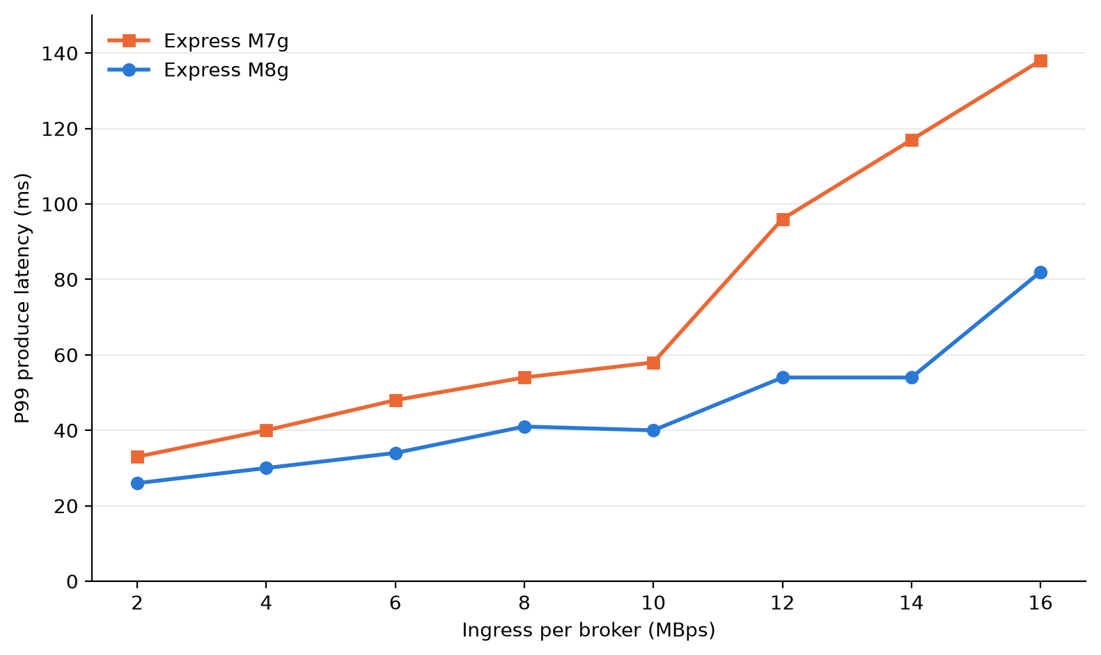
Figure 1: Client P99 produce latency by ingress per broker for express.m8g.large and express.m7g.large
At the same load, M8g brokers used less CPU. Broker CPU (user plus system, averaged across the three brokers) was 9–11 percentage points lower on M8g at each step. At 6 MBps per broker, M8g ran at 45 percent and M7g at 56 percent. M7g brokers ran at 60 percent or higher from 8 MBps per broker. M8g brokers stayed below 60 percent through 14 MBps per broker. That gives you more room on each broker for traffic spikes and broker maintenance.
| Ingress per broker (MBps) | M8g CPU (%) | M7g CPU (%) |
| 2 | 39 | 49 |
| 4 | 41 | 52 |
| 6 | 45 | 56 |
| 8 | 51 | 61 |
| 10 | 51 | 60 |
| 12 | 56 | 66 |
| 14 | 58 | 68 |
| 16 | 62 | 72 |
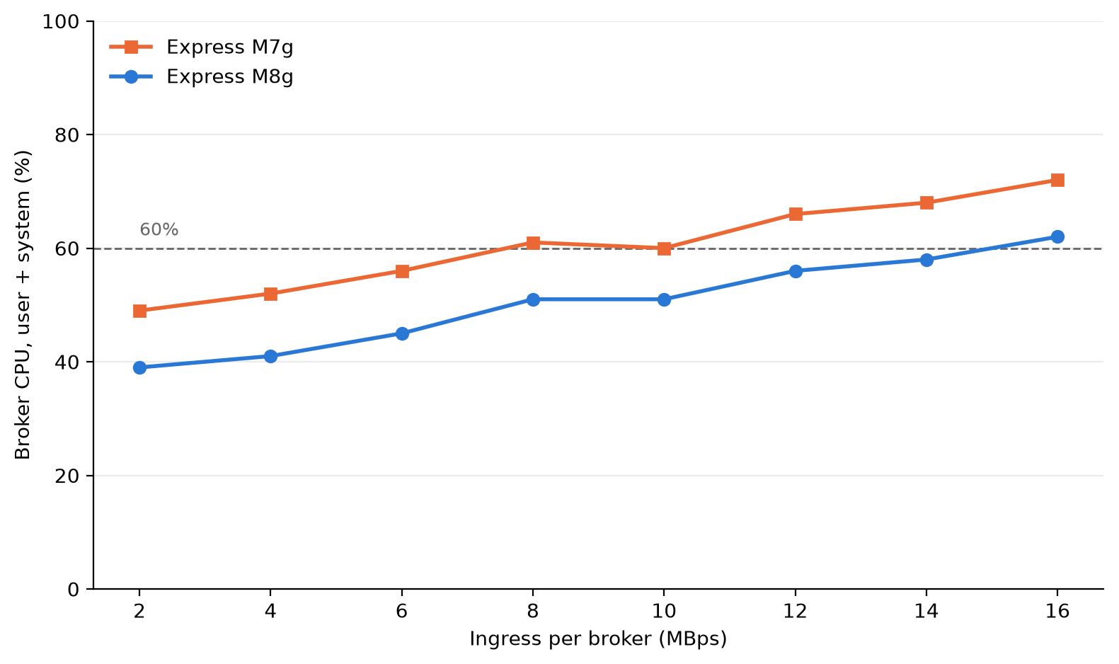
Figure 2: Average broker CPU (user plus system) at each load step for express.m8g.large and express.m7g.large
When consumers fall behind, for example after an outage or a deployment, they must read the backlog while producers keep writing. We ran a separate test to measure how fast consumers catch up on each generation. This test used a new pair of express.m8g.large and express.m7g.large clusters, with the same Kafka version, authentication, and encryption as the latency test, and the following differences:
acks=all, batch.size=65536 (64 KiB), linger.ms=10, and compression.type=none.With a backlog of about 30 million records (about 30 GB), consumers on M8g caught up in 13–18 minutes. On M7g, consumers had not caught up after 30 minutes and still had 2–9 million records to read. At the largest backlog, about 120 million records, consumers on M8g cleared about 91 million records in 30 minutes, compared with 30–32 million on M7g. That is about 3x more backlog cleared in 30 minutes.
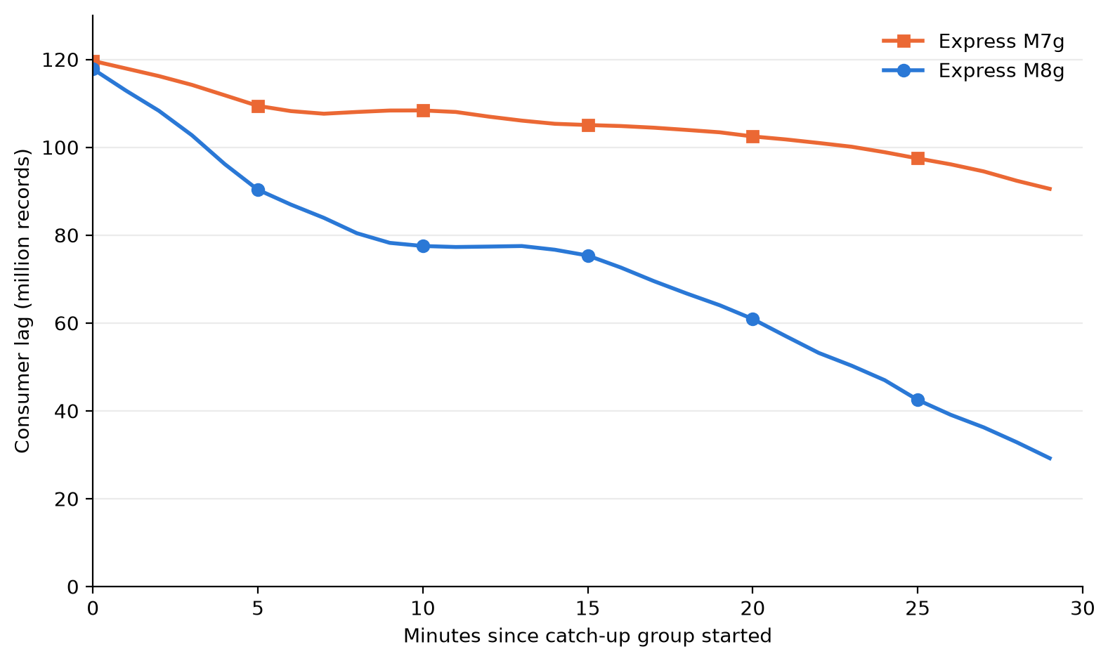
Figure 3: Consumer lag after a catch-up group starts from the earliest offset of a 120-million-record backlog, for express.m8g.large and express.m7g.large
Your results depend on load, message size, batch settings, consumer group count, and broker size. We ran this test on the large size only. To estimate your results, create an Express cluster on M8g and run your own workload against it. When you finish testing, delete the cluster to avoid ongoing charges.
Express brokers on M8g lower your costs in two ways: lower broker-hour pricing, and no broker-side charge for cross-AZ client traffic.
Broker-hour pricing for Express brokers on M8g is 15 percent lower than Express brokers on M7g at each size. In US East (N. Virginia), express.m8g.large costs $0.347 per hour and express.m7g.large costs $0.408 per hour. Data-in and storage pricing don’t change.
Many production Kafka clusters run across three Availability Zones. When a client connects to a broker in a different Availability Zone, the traffic between them is cross-AZ traffic. With clients spread evenly across three Availability Zones, about two-thirds of client traffic is cross-AZ. Each request goes to the partition leader, which can be in any Availability Zone.
Standard AWS data transfer charges for cross-AZ traffic in US East (N. Virginia) are $0.01 per GB on the sending side and $0.01 per GB on the receiving side, or $0.02 per GB in total. With Express brokers on M8g, AWS doesn’t charge the broker side, so cross-AZ traffic between your clients and brokers costs $0.01 per GB in total. That’s 50 percent lower than on M7g.
The following table shows the cross-AZ data transfer charge per GB of client traffic for each generation.
| Express on M7g | Express on M8g | |
| Client side | $0.01 per GB | $0.01 per GB |
| Broker side | $0.01 per GB | Not charged |
| Total per GB of cross-AZ client traffic | $0.02 | $0.01 |
You can reduce consumer cross-AZ traffic with rack awareness. Producers must write to the partition leader, which can be in any Availability Zone. Consumers can read from a replica in their own Availability Zone instead. To turn this on, set replica.selector.class to org.apache.kafka.common.replica.RackAwareReplicaSelector in your cluster configuration. Set client.rack on each consumer to the Availability Zone ID it runs in (for example, use1-az1). Consumers that read from a local replica don’t incur cross-AZ traffic, so you pay cross-AZ charges only on the produce side. On Express brokers on M8g, that produce-side cross-AZ traffic costs $0.01 per GB. If you don’t use rack awareness, your consumer cross-AZ traffic also costs 50 percent less on M8g, because AWS doesn’t charge the broker side.
For example, consider a cluster of three large brokers in US East (N. Virginia) with 30 MBps of ingress and two consumer groups (60 MBps of egress). Over a 30-day month, about 155,520 GB of client traffic crosses Availability Zones.
| Monthly cost | Express on M7g | Express on M8g | Express on M8g with rack awareness |
| Broker hours (3 brokers × 720 hours) | $881.28 | $749.52 | $749.52 |
| Cross-AZ produce traffic (51,840 GB) | $1,036.80 | $518.40 | $518.40 |
| Cross-AZ consume traffic (103,680 GB) | $2,073.60 | $1,036.80 | $0 |
| Total | $3,991.68 | $2,304.72 | $1,267.92 |
With rack awareness, the cross-AZ charge in this example drops from $1,555.20 to $518.40 per month. Reading from a follower replica can add a small amount of end-to-end latency, so test with your workload. For setup steps, see Reduce network traffic costs of your Amazon MSK consumers with rack awareness.
Data-in and storage charges are the same on both generations, so they aren’t included.
To estimate your own cross-AZ traffic, add the BytesInPerSec and BytesOutPerSec CloudWatch metrics across your brokers. Each 1 MBps sustained over a 30-day month is about 2,592 GB. Multiply the total by two-thirds if your clients are spread evenly across three Availability Zones. If your consumers use rack awareness, count only BytesInPerSec.
This applies only to traffic between your clients and brokers. Replication traffic between brokers, and between metadata nodes and brokers, isn’t charged on either generation. For details, see Amazon MSK pricing.
You have three options, depending on where your workload runs today.
In the Amazon MSK console, choose Create cluster, choose Express as the broker type, and choose an M8g size. You can also use the CreateClusterV2 API.
You can change the broker type of a cluster from M7g to M8g in place. Amazon MSK updates brokers one at a time, so clients keep producing and consuming during the update.
Before you update, check that your partition count per broker and your throughput fit within the limits for the target size.
Create a new Express cluster on M8g, and then use Amazon MSK Replicator to copy your topics, data, and consumer group offsets to it. For steps, see Migrate from Standard brokers to Express brokers or Migrate from non-MSK Apache Kafka clusters.
Express brokers on Graviton4-based M8g instances lower the cost of running Kafka on Amazon MSK and lower tail latency for the same load. You get 15 percent lower broker-hour pricing, no Amazon MSK broker-side charge for cross-AZ client traffic, and a 24xlarge size for workloads that need more capacity per broker. In our benchmark at the large size, P99 produce latency was 21–54 percent lower, broker CPU was 9–11 percentage points lower, and consumers that fell behind cleared up to 3x more backlog in 30 minutes than on M7g.
To get started, create an Express cluster on M8g or update your Express cluster on M7g. Amazon MSK supports M8g sizes in every AWS Region that supports Express brokers. For pricing, see Amazon MSK pricing. For setup steps, see the Amazon MSK Developer Guide.
If you have questions or feedback, leave a comment on this post or start a thread on AWS re:Post.
Post Syndicated from The Atlantic original https://www.youtube.com/shorts/Ne50034TCYc
Post Syndicated from Crosstalk Solutions original https://www.youtube.com/shorts/VqBNMakTRWo
Post Syndicated from The Atlantic original https://www.youtube.com/shorts/rqArc8-rW4Q
Post Syndicated from Meriem SMACHE original https://aws.amazon.com/blogs/security/securely-exposing-amazon-bedrock-agentcore-runtime/
Amazon Bedrock AgentCore Runtime delivers a secure serverless environment to deploy AI agents and tools at scale. When you start talking to your agent, the runtime launches a dedicated isolated session that runs in its own dedicated microVM with a completely sandboxed CPU, memory, and filesystem allocation. This provides strict data governance, helps to prevent cross-tenant data leakage, and preserves context while isolating stateful reasoning from external sessions.
To govern access control across these environments, Amazon Bedrock AgentCore Identity provisions distinct workload identities to let your agents run. By federating directly with an OpenID Connect identity provider like Amazon Cognito, Okta, or others, the users can only see and interact with agents they’re authorized to use.
But securing the runtime alone doesn’t protect the ingress path perimeter. When you expose your agent to users through a web or mobile application, the AWS Shared Responsibility Model dictates that you should provide a dedicated access layer that enforces tight control over the origin and intent of every request before any traffic reaches the runtime.
The access layer acts as a trusted bridge to authenticate each incoming request, enforce authorization rules, preserve user identity through the request lifecycle, and securely channel all user traffic into the isolated runtime.
This post walks through two architectures for securing access to AgentCore Runtime and provides guidance to help you decide which architecture best fits your organization.
In an agentic workflow, downstream data access should remain tied to the invoking user’s identity, and each segment in the execution chain is permissioned only for the immediate next hop. Using a single static credential, even one linked to the original requester, grants every immediate component identical, broad access. This directly violates the principle of least privilege, because the ingress gateway, the proxy, and the agent’s tool execution context each require only enough permission to reach the next component.
Recent real-world incidents have demonstrated that agentic workloads can bypass internal prompt guardrails, escape the software sandboxes, and abuse static credentials to move across applications and layers. In a multi-chain agentic architecture, scoping each hop as tightly as possible is key to preventing these exploits.
However, long-running, unattended execution poses a fundamental identity challenge for extended agentic workloads. If an agent runs a complex task that takes hours, the user’s interactive session will expire before the workload ends, making their short-lived OAuth 2.0 access token invalid mid-execution. Refreshing the tokens won’t solve this problem and storing a long-lived, user-scoped credential inside the agent’s runtime environment might reintroduce exactly the broad, standing credential attack surface that the zero-trust architectures are intentionally designed to mitigate.
To mitigate this, identity propagation acts as a critical bridge between authentication at the perimeter and authorization at the data layer. The agent must operate within the invoking user’s authorization scope. Every session receives a short-lived, user-scoped token that provides only the permissions granted to that specific user and authorization is enforced at each hop. If any single segment is compromised, then the exposure is contained in that hop scope. This security model also strengthens a continuous verification process where the tokens are validated at every hop from the ingress endpoint through AgentCore to the downstream resource, so no segment operates with unverified or elevated privileges.
We explained in the previous section why identity must follow the user through every hop. However, identity propagation alone isn’t enough to secure the ingress path; it must be integrated within a broader set of ingress controls that together protect the path into the runtime.
AgentCore Runtime provides infrastructure isolation, per session microVMs, per session tool registration, and enforces the application of Amazon Bedrock Guardrails. These features and resources protect the execution environment. However, they don’t control who reaches the runtime, how they’re authenticated, or whether their identity is preserved through the chain. That responsibility falls on the ingress control layer that you build. Securing this path requires a defense-in-depth architecture that binds every request to the user’s identity before it ever reaches the agent’s reasoning loop.
To protect and control data access, any architecture exposing AgentCore Runtime to users must satisfy the following requirements:
These security requirements are mandatory baselines to expose any agentic workloads to users. Any missing requirement might create a potential attack vector. By applying this full set of guardrails, you help contain the impact of a potential malicious exploit to a single user, a single session and a single execution hop.
In the next section, we provide two architecture patterns that implement this propagation differently:
Both approaches achieve the same result: the agent acts as the user rather than with elevated privileges.
Each of the following patterns is presented the same way: the layered controls a request passes through before reaching the agent, followed by how user identity is carried to the runtime. As you explore, please note where each pattern places the trust boundary as that difference is what drives the trade-offs summarized at the end.
We expose AgentCore Runtime through Amazon API Gateway, which acts as a dedicated ingress point that terminates each client connection. Before any request reaches the agent, it must pass through layered security controls:
Because the client-provided session ID is treated as untrusted input, the Lambda authorizer creates a composite session ID by appending the user identifier to the client-provided session ID. Even if two different users submit the same session ID, they resolve to unique composite IDs at the AgentCore Runtime level, preventing any cross-user session leakage.
To prevent denial of service attempts, we suggest using Amazon DynamoDB as a lightweight session counter. While the AWS WAF rate-based rules attached to the API Gateway stage protect against IP-level volumetric abuse, they evaluate requests before authentication. The Lambda authorizer checks and increments a per-user counter in DynamoDB after validating the user’s identity, helping prevent a single authenticated user from exhausting agent capacity, even if they connect from multiple IP addresses. This design scales cleanly by using a composite session ID. The Lambda Authorizer combines the user identifier and the client session ID, routing each user’s counter to a distinct partition. This naturally distributes write traffic and reduces the risk of hot keys.
Each session can sustain roughly 1,000 counter updates per second before reaching DynamoDB’s per-partition write limit, which is far beyond what any legitimate session would ever generate. That same limit is exactly what makes the counter an effective throttle. Meanwhile, total capacity across all users scales horizontally, growing with the number of active sessions. For high-volume production deployments, on-demand capacity mode absorbs sudden spikes automatically, and CloudWatch Contributor Insights lets you confirm traffic stays evenly distributed.
After the Lambda authorizer approves the request, as shown in the Figure 1:
API Gateway forwards the request to a Lambda proxy running on a private VPC with no internet egress. The role of this Lambda proxy is to relay the request to AgentCore Runtime through a VPC endpoint, so that all communication remains within the private network. The Lambda proxy forwards the user’s token (unchanged) in the Authorization header, which preserves the user’s identity all the way to AgentCore Runtime.
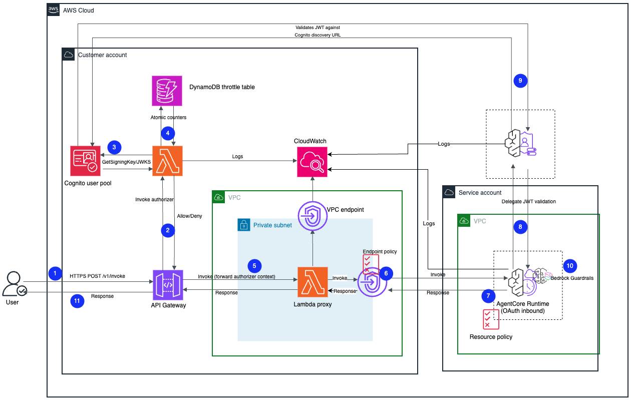
Figure 1: Pattern A architecture for exposing AgentCore Runtime through Amazon API Gateway
This VPC endpoint enforces a strict network perimeter using two independent controls:
"*" and a condition that allows invocations only when the request carries aws:SourceVpc and aws:SourceVpce values matching this stack’s VPC and endpoint. Authentication happens at the AgentCore Identity level, so there is no AWS Identity and Access Management (IAM) principal to match, and the network path is the only meaningful gate and condition that remains. AgentCore Runtime rejects requests sent directly from outside the VPC with an AccessDeniedException, even with a valid JWT.Beyond the network boundary, Amazon Bedrock Guardrails evaluates each model’s invocation for prompt injection attacks, helping catch malicious inputs even after an invocation has passed identity and network verification. This adds content protection as a defensive layer independent of identity and network controls.
Your stack logs and tracks every authorization outcome along this path as structured JSON to Amazon CloudWatch, with an INVALID_JWT alarm. The full walkthrough and a deployable AWS Cloud Development Kit (AWS CDK) sample are linked at the end of this post.
Before production deployment, we recommend configuring an AWS WAF Web ACL at the API Gateway stage to inspect requests before they reach the Lambda authorizer. You should include AWSManagedRulesCommonRuleSet and AWSManagedRulesKnownBadInputsRuleSet for generic OWASP Top 10 protections and known exploit patterns, AWSManagedRulesSQLiRuleSet to catch injection signatures, a per-IP rate-based rule ahead of the DynamoDB throttle counters, and custom rules to reject oversized requests or malformed session IDs early. For a step-by-step integration guide including two deployment patterns for placing AWS WAF in front of the AgentCore Runtime, see Securing Amazon Bedrock AgentCore Runtime with AWS WAF.
This first pattern satisfies the ingress security requirements discussed earlier. It achieves defense in depth by applying the authentication at two independent layers, enforcing authorization through session binding and controlling traffic through per-user throttling. The architecture maintains per-hop least privilege from the API Gateway through the AgentCore Runtime while preserving end-user identity propagation by passing the user’s token through unchanged. The edge filtering is managed with AWS WAF and the network perimeter is enforced by VPC endpoint controls. The design includes the application of Amazon Bedrock Guardrails for content security with a tamper-proof audit trail in Amazon CloudWatch. The deployable CDK sample for pattern A is available on GitHub.
With Pattern B, you expose AgentCore Runtime through Amazon Bedrock AgentCore Gateway, a managed service purpose-built for agentic traffic that combines ingress authentication, token exchange and Runtime routing without requiring a proxy Lambda function or custom VPC networking.
Before any request reaches the agent, it passes the following layered security controls:
After the authorization succeeds, the gateway manages the outbound call to AgentCore Runtime by using a strict workload isolation mechanism as shown in Figure 2:
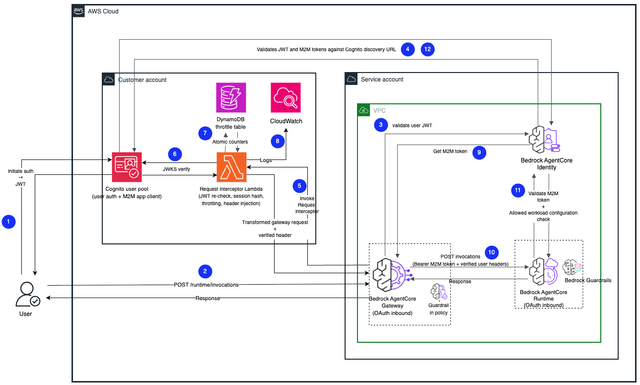
Figure 2: Pattern B architecture for exposing AgentCore runtime through AgentCore Gateway
If a client attempts to bypass the gateway by sending a valid user token directly to the runtime, the request is automatically rejected because it lacks the required workload identity.
For more operational efficiency, AgentCore Gateway integrates AWS WAF directly at the single gateway access point, protecting the entire ingress path in one place, without the need to manage separate authorizers, proxy Lambda functions or VPC endpoints.
While API Gateway also supports AWS WAF, the AgentCore Gateway pattern simplifies management by consolidating all ingress controls behind a single component.
The AgentCore Gateway also supports native rate limiting, removing the need for custom DynamoDB-based throttle tables, for your production environments. The interceptor writes a structured audit trail to CloudWatch, with an INVALID_JWT alarm to flag spikes in authentication failures.
Before production deployment, we strongly recommend that you enable AWS WAF on the AgentCore gateway with the same rule sets described in the API Gateway pattern, including the OWASP protections, SQL injection, and custom rules for oversized or malformed requests.
To summarize, this second architecture satisfies the ingress security requirements defined earlier. It achieves defense in depth by applying a managed CUSTOM_JWT authorizer directly at the entry point, enforcing authorization through interceptor-based session binding and using rate limiting to control traffic. This pattern maintains per-hop least privileges from AgentCore Gateway through to the runtime by automating M2M token exchange, while propagating user identity for on-behalf-of execution. The edge security is managed by AWS WAF, coming directly with the gateway’s single-entry point, and secure workload isolation strictly enforces the perimeter. Finally, this design applies declarative Amazon Bedrock Guardrails for early content safety, and a tamper-proof audit trail and alarms in CloudWatch. The complete CDK sample for Pattern B is available on GitHub.
As explained earlier, securing access to AgentCore Runtime can be achieved through two different patterns: The AgentCore Gateway pattern or the Amazon API Gateway pattern. The right choice depends on your existing AWS infrastructure, workload constraints, and operational preferences.
Choose the Amazon API Gateway pattern if:
Choose the AgentCore Gateway pattern if:
The following table summarizes the key elements that help you make the right architectural decision:
| Consideration | API Gateway (Pattern A) | AgentCore Gateway (Pattern B) |
| Suited to | Teams already standardized on API Gateway | Teams starting fresh who want less infrastructure to operate. |
| Perimeter control | Runtime resource policy with aws:SourceVpc and VPC endpoint security group | Runtime workload lock (allowedWorkloadConfiguration). |
| Components to operate | API Gateway, Lambda authorizer, Amazon VPC, VPC endpoints, proxy Lambda function | AgentCore Gateway and Lambda REQUEST interceptor. |
| User identity to agent | User JWT forwarded unchanged (no SigV4) | Interceptor-injected verified headers (OAuth outbound M2M token). |
| AWS WAF | Attach directly to the API stage | Attach directly to the gateway. |
| Request timeout | Inherits the API Gateway integration timeout | Not subject to this limitation. |
| Public endpoint | Can be fully private (API Gateway PRIVATE endpoint type) | Supports AWS PrivateLink ingress and VPC Lattice egress, but keeps a public endpoint active. Access relies on the JWT authorizer and resource policy rather than removing the endpoint |
By securing access to the AgentCore Runtime with a defense in depth, an agent can be both highly usable and secure. The two patterns in this post complete the shared responsibility model for you: they authenticate every request against the identity provider, authorize it at each step and propagate the user’s identity end-to-end from the edge through the token exchange into the isolated microVM (AgentCore Runtime) and down to the agent’s tool calls (AgentCore Gateway). Each step only holds a short-lived credential for the next one, so the agent always works within the user’s permissions rather than with broad, long-term access. If one step is ever compromised, the design limits the impact to that single step, session and user. Whether the runtime is behind API Gateway with a VPC endpoint or in front of it with AgentCore Gateway, the design verifies each request at each step.
To get started, clone the Pattern A sample or the Pattern B sample, deploy it in your account, and test it against your requirements. Both samples are provided as a starting point, not a production-ready deployment. We recommend working with your security and legal teams to adapt to the controls before going live. From there, you can extend either pattern for multi-tenant use, add observability hooks, or tighten controls for your specific compliance requirements.
If you have questions about this post, contact AWS Support or start a new thread on AWS re:Post.
Post Syndicated from Patrick Nemeroff original https://blog.cloudflare.com/quad9-withdrawal-from-france/
Last month, the Swiss non-profit foundation Quad9 announced that it will withdraw its free public DNS resolver from France. This difficult decision followed months of litigation and a French court ruling that imposed daily financial penalties on Quad9 for failing to block domains associated with alleged copyright infringement.
Quad9’s departure from France is both disheartening and understandable. The court’s ruling put the organization in the impossible bind of having to choose between crippling litigation and penalties, or fundamentally altering its service in a way that would undermine the privacy and security of its users. Left with no good option, Quad9 is choosing the exit door instead.
The withdrawal of a basic infrastructure service from France fundamentally harms the free and open Internet, and it should serve as a warning of the damage that will result if rightsholders and policymakers continue demanding maximal blocking across every layer of the Internet. It not only deprives French Internet users of a trustworthy and important tool; it creates a real risk of disruption to their daily lives. Quad9’s resolver is used by a wide variety of individuals and organizations in France — including government bodies, educational institutions, hospitals, and utilities — and Quad9 has no way to directly notify those individuals and institutions that their resolver will soon stop working. If the affected parties do not change their resolver before Quad9 removes its service, their Internet will fail with no explanation.
Quad9 is not the first public DNS resolver to withdraw from a country following blocking orders, and it almost certainly won’t be the last. Cisco previously withdrew its OpenDNS resolver from France, Portugal, and Belgium (temporarily) under similar circumstances. And a Belgian court recently issued an order that would impose substantial penalties if Cloudflare, Google, and Cisco do not begin blocking websites through their public resolvers by early January 2027. That’s something Cloudflare has never done.
Cloudflare has spent years advocating against orders of this kind. We are concerned that rightsholders’ unrelenting demands for blocking by public DNS resolvers will end up causing real harm to the Internet.
To understand why this is such a problem, it helps to understand how the Internet works under the hood. DNS resolvers are a foundational piece of the Internet’s infrastructure. DNS is the Internet’s address book: when you type a website name such as cloudflare.com, the DNS system translates that domain name into the IP address your device needs to connect to it. A DNS resolver is the service that looks up that address and sends it back to your device, much like an operator finding a phone number in a directory.
DNS resolvers can be operated by anyone, but they are commonly run by Internet service providers (ISPs), mobile networks, businesses, and universities. If you’re reading this blog post at home and have never thought about DNS before, chances are that you’re using your ISP’s default resolver. Because you use your DNS resolver every time that you visit a website, it’s important for it to be reliable and trustworthy.
And because the DNS resolver has access to all of your browsing activity, which resolver you use has real privacy implications.
In addition to DNS resolvers that are provided by your local ISP, there are a variety of public DNS resolvers available. Cloudflare launched our public DNS resolver 1.1.1.1 in April 2018 to give back to the Internet. Our goal was to make a fast, reliable, privacy-first consumer DNS service available for free to everyone. We succeeded. 1.1.1.1 is among the fastest DNS resolvers in the world, including in Europe. Cloudflare's resolver doesn’t collect any user data, let alone sell it to advertisers. 1.1.1.1 has always been one of our favorite examples of Cloudflare fulfilling its mission to help build a better Internet.
1.1.1.1 is one of many public resolvers that anyone can use. In addition to 1.1.1.1 and Quad9’s 9.9.9.9, some of the other best-known public resolvers include Google’s 8.8.8.8 and Cisco’s OpenDNS. Just because these services are offered for free doesn’t mean they’re easy to provide. A well-run global public DNS resolver is an extraordinary engineering feat, built to securely and privately resolve hundreds of billions or even trillions of queries a day across a globally distributed network of hundreds of server locations.
As Quad9 notes, there are many other DNS resolvers available to users, many of them offered by essentially anonymous services whose practices are unknown or undocumented. It’s easy to change your DNS resolver, and people do so for a variety of reasons including performance, reliability, or to access specific security features.
Rightsholders have a legitimate interest in preventing online piracy. But trying to address online infringement through public DNS resolvers is fundamentally the wrong approach.
Among other things, such blocking is ineffective. Think back to the analogy of an operator finding a phone number in a directory. If a court wants to shut down an illegal business, forcing the directory operator to cross the business's name out of the phone book doesn't actually close the business. The storefront is still open, the products are still there, and anyone who already knows the address, or uses a different phone book, can walk in.
The same is true for the Internet. DNS resolvers are just one link in the transmission chain. The only way a DNS resolver can “block” content is by declining to return the IP address for a particular website. But a public DNS resolver cannot remove the actual infringing content from the Internet, nor can it take down the servers hosting it.
Because of this, blocking by public DNS resolvers is remarkably easy to bypass. Any Internet user who wants to reach a blocked site can circumvent the block in less than a minute simply by switching to one of the thousands of other DNS resolvers available online. In fact, users don’t even need a resolver at all to reach infringing content if they already know the underlying IP address. Unsurprisingly, while blocking via public resolvers may inject some friction for some users when accessing content, there is no evidence that it actually reduces the total amount of online infringement that occurs.
In addition to being ineffective, as we’ve written previously, DNS blocking is a blunt instrument that causes collateral damage. Because DNS operates at the domain level, a resolver cannot block a specific infringing video or file; it must block the entire domain. This affects all content on that domain, whether legal or illegal. It is also entirely opaque to the user: when a resolver is forced to block a domain, the website simply fails to load. The user receives no explanation or legal notice, making it impossible to know if the site is down for maintenance, if their network is broken, or if the site was blocked by a court order.
The problem is substantially worse with respect to public DNS resolvers. Because public resolvers operate globally, any blocking will naturally cross borders, meaning that a single country could dictate what content is accessible around the world. For example, while the EU-dedicated DNS resolver DNS4EU operated by Whalebone blocks in response to country-specific orders, it does so across the entire EU. Efforts to reengineer public DNS resolvers to allow for more localized blocking would fundamentally alter the service, harming performance and resilience, undermining user privacy, and fragmenting the open Internet.
For these reasons, Cloudflare, Google, Cisco, and Quad9 have all opposed efforts to mandate blocking by public DNS resolvers, with some success. Several years ago, courts in Germany ruled in favor of Cloudflare and Quad9, rejecting requests to require DNS blocking. More recently, a French court rejected penalties against Cloudflare for failing to block through 1.1.1.1, finding that other actions we had taken through our CDN and reverse-proxy service were sufficient to comply with the underlying order.
Undeterred, rightsholders have continued to press for blocking by public resolvers with a level of determination that is hard to explain. A recent study found that the majority of online piracy in Europe is hosted in Europe. If rightsholders want to genuinely address online infringement, there are far better places to focus their efforts — most notably by requiring the hosting providers who actually store the pirated files to take them down.
The French court’s penalty order against Quad9 represents the culmination of these rightsholder efforts. As a small non-profit that only offers a public DNS resolver, Quad9 had no alternative methods for demonstrating compliance with the order. The French court therefore granted rightsholders’ request to issue penalties for non-compliance, forcing Quad9 to undermine its own service or leave the country.
Quad9’s withdrawal from France represents a genuine loss for the Internet. In the short term, removal of Quad9’s resolver is likely to cause immediate and potentially severe disruptions to Internet access. Because of the way their service is set up to preserve privacy, Quad9 has no way to know who exactly is using its resolver, let alone to directly communicate to them about the upcoming withdrawal of services. That means that individuals, hospitals, universities, and government offices all may be caught unaware when the resolver stops working. Again, because of how DNS resolvers work, those users will not receive a detailed error message explaining what happened — their Internet will simply stop working. The problem will be even worse when devices like security systems or thermostats are hardwired to use Quad9’s resolver. Fixing these issues may be slow or even impossible.
More generally, driving Quad9 out of France does absolutely nothing to prevent online infringement, but it does leave everyday Internet users with fewer safe, reliable options, particularly ones like Quad9 that also protect users from phishing and malware. Taking established public DNS resolvers away forces Internet users to fall back on the default resolvers offered by their ISPs (which may monetize their browsing data), try lesser-known resolvers operated by anonymous or less trustworthy organizations, or run their own resolver. The irony is that Quad9 and Cloudflare are being pulled into court precisely because we are transparent, reputable organizations. Penalizing transparent services only pushes users toward less accountable corners of the web.
If nothing else, we hope that Quad9’s announcement may serve as a wake-up call to rightsholders and policymakers that seeking to block infringement at every layer of the Internet has real costs.
We believe there are far better ways to work together to fight piracy without compromising the integrity of the Internet, and Cloudflare continues to pursue innovative collaborations to that end. Our collective efforts in addressing online infringement would be put to better use in seeking to have such content removed at the hosting provider, which would both achieve a more durable solution and avoid collateral damage to the Internet.
In the meantime, we will keep resisting misguided efforts to require blocking by public DNS resolvers. Along with Google and Cisco, we have appealed the Belgian order that would impose penalties on us if we do not start DNS blocking by January 2027. We hope to get a resolution before the end of the year that would avoid another situation like the one Quad9 faces now in France.
We have grave concerns about the disruption that would be caused if additional resolvers are forced to withdraw from markets, and we will continue to advocate against that possible result.
Post Syndicated from Биволъ original https://bivol.bg/deutschebank_trump.html

Международното журналистическо разследване Inside Deutsche Bank („Отвътре в Deutsche Bank“) разкрива финансовите връзки на компаниите на Тръмп със схемата за пране на пари “Азербайджанска перачница”. Компаниите на Тръмп са получили…
Материалът <span style='color:#ff0000;font-size:12px;'>Inside Deutsche Bank:</span> <BR> <H1 class='post-title single-post-title entry-title'>Тръмп, Deutsche Bank и руската връзка</H1> е публикуван за пръв път на Bivol!.
Post Syndicated from Arik Yakir original https://aws.amazon.com/blogs/devops/enforcing-zero-trust-dependency-policies-in-aws-codebuild-with-jfrog-curation/
Software supply chain attacks are rising sharply. JFrog’s 2026 research recorded a 451% year-over-year increase in malicious npm packages, yet every application that pulls open source packages during a build is still taking the same fundamental risk. When a developer runs pip install or npm install, the build environment downloads dependencies directly from public registries with no verification that those packages are safe. A vulnerable or malicious package can slip into your container image, get pushed to a registry, and reach production before anyone notices. By the time a scanner flags a critical CVE, the damage is already done.
This is a familiar situation for teams building on any continuous integration and continuous delivery (CI/CD) platform, including AWS CodeBuild. A build completes successfully, tests pass, and the artifact ships. Days or weeks later, a security review reveals that one of dozens of transitive dependencies carried a known vulnerability, or worse, was a malicious package designed to exfiltrate secrets. The fix isn’t only patching. It’s rebuilding, re-testing, and redeploying, all while assessing the scope. What teams need is a way to enforce a zero-trust dependency policy: a gate that blocks risky packages at download time, before they ever enter the build. That is exactly what JFrog Curation provides. It evaluates every package at the moment it is downloaded. When a package violates policy, it returns an HTTP 403 (Access Denied) error, failing the build before a risky dependency enters your environment.
In this post, you’ll learn how to use JFrog Curation as a policy gate inside AWS CodeBuild to block vulnerable and malicious dependencies at download time, before they ever become an artifact.
Your team ships a container built from open source dependencies. Weeks later, a security scan surfaces a critical vulnerability in a transitive package you didn’t even choose. Now you’re scrambling to identify which images are affected, rebuild, re-test, and redeploy, all under time pressure and with no guarantee you’ve caught everything.
The root cause is that nothing enforces policy at the moment dependencies are downloaded. When a build runs pip, npm, or Maven, it pulls whatever the manifest declares directly from a public registry. Scanning catches problems after the artifact exists, but by then the vulnerable package is already in your image and potentially in production.
The pipeline is an ordinary container build with one decisive change: The only route to public package registries runs through JFrog Artifactory, and Curation sits on that route. A developer commit triggers CodeBuild, which runs a Docker build. Inside that build, pip install resolves through the Artifactory virtual repository. Approved packages flow through and the image is pushed to Amazon Elastic Container Registry (Amazon ECR). A blocked package fails the build before any image exists.
For this walkthrough, the policy is “Block Critical CVEs”, which rejects any package version with a Common Vulnerability Scoring System (CVSS) score of 9.0 or above. AWS CodeBuild is the orchestration layer that resolves dependencies, and JFrog Curation is the management layer that decides, package by package and in real time, what CodeBuild is allowed to pull. The result is an Amazon ECR repository that receives only images built from policy-compliant dependencies.
On failure, a small amount of post-build scripting (shown in detail in the post-build section) queries the Curation audit API (JFrog Curated Packages Audit Events service) and reports the blocked package, its CVE identifiers and CVSS scores, and any recommended fix versions.
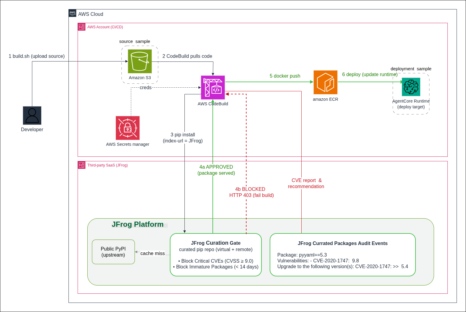
Figure 1: Deployment architecture for the AWS CodeBuild pipeline with JFrog Curation security gate
Before starting the walkthrough, make sure you have the following accounts, tools, and permissions in place.
https://pypi.org.The pipeline is deliberately small. A handful of shell scripts are orchestrated by a CodeBuild buildspec.yml and a Dockerfile that does the dependency install. What makes it a security gate rather than a build is one design choice. Every pip install is forced to resolve through a curated JFrog repository instead of public PyPI and the build is only allowed to publish an image when Curation approves every package.
The following shows how the pieces fit together before we look at the code:
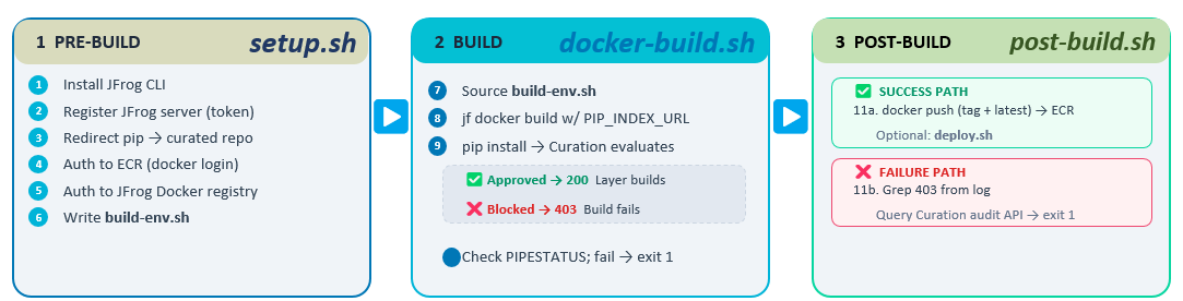
Figure 2: CodeBuild pipeline phases and script responsibilities
| File | Role |
buildspec.yml |
CodeBuild entrypoint – wires the three phases together and sets shared env vars |
scripts/setup.sh |
Pre-build: installs the JFrog CLI, loads secrets, configures pip + Docker auth |
| Dockerfile | Defines the image. Its pip install is what actually gets curated |
| requirements.txt | The pinned dependency manifest that Curation evaluates, package by package |
scripts/docker-build.sh |
Runs the curated Docker build and captures the log |
scripts/post-build.sh |
The gate: conditional push to the registry, or extract-and-report the block reason |
The buildspec keeps logic out of YAML and in versioned shell scripts to keep the pipeline testable locally and readable in review. Two details matter beyond the phase wiring:
shell: bash is set explicitly. CodeBuild defaults to sh, and the post-build gate relies on bash-only constructs like ${PIPESTATUS[0]}.This phase does three jobs: install the JFrog CLI, authenticate to both registries, and reconfigures pip so it resolves through Artifactory.
Importantly, jf pip-config writes a pip config that swaps the default index URL pypi.org for the JFrog virtual repo. From that point on, any pip install, including the ones inside the Docker build, asks Artifactory for packages. Artifactory serves approved packages from cache or fetches them from its PyPI remote, and returns an HTTP 403 (Access Denied) error for anything a Curation policy blocks. The application code never changes. The redirection is entirely in configuration.
The following is the full Dockerfile:
The gate is the pip install -r requirements.txt step and the mechanism is --index-url. During the build phase, docker-build.sh passes the curated JFrog index URL into the build as PIP_INDEX_URL. When that argument is present, pip resolves all dependencies in requirements.txt through the curated JFrog repository instead of public PyPI. JFrog evaluates each requested name==version against your Curation policies before it serves the package:
Approved packages are returned normally and the layer builds. Blocked packages get an HTTP 403 (Access Denied) error from JFrog. pip treats that as a failed download, the RUN instruction exits non-zero, and the entire docker build fails. The image is never produced, let alone pushed. The policy decision is made during the image build process at the precise moment pip resolves each dependency against the curated JFrog repository.
The post-build phase decides what happens with the build’s result. It branches on the CODEBUILD_BUILD_SUCCEEDING flag that CodeBuild sets, which is the mechanism that ties the registry push to Curation’s verdict:
Note the source /tmp/build-env.sh at the top. Each phase script runs in its own subshell, so values derived earlier (like ECR_URI) don’t survive across phases. The pre-build step writes them to a file that this script reads back in. If every dependency was approved, the script pushes the trusted image to ECR (both the build’s tag and latest) and triggers the downstream deploy stage. Configure it like so:
This is the only path that puts an image in the registry.
If curation blocked a package and pip only surfaced an HTTP 403 (Access Denied) error, the script reconstructs the reason in three steps. First, identify the package by grepping the failing 403 out of the captured build log. pip names the package in the download URL:
Second, ask the Curation audit API which policy fired for that package (the policy name, the matched condition, and the category):
Third, run jf curation-audit for a human-readable explanation and a recommended compliant version:
(That last step is also where any CVE detail comes from, but only when the remote repo has pass-through for Curation audit enabled.)
Finally, the script fails the build:
The logic is deliberate: the push is gated on the build succeeding, and the build only succeeds if Curation approved every dependency.
On the blocked path, the build declares pyyaml==5.3, which carries two CVSS 9.8 vulnerabilities. Curation returns HTTP 403 (Access Denied) and the build fails before an image is ever produced:
Nothing reached Amazon ECR. There is no vulnerable artifact to remediate, because it was never built.
JFrog Curation is the prevention layer at the gate, and JFrog Xray, a software composition analysis (SCA) tool, is the detection layer for what is already inside. Together they cover both new downloads and previously cached artifacts.
This pattern is workload-agnostic. The example builds a container, but the same gate applies equally to your AWS Lambda function, microservice, or front-end application that resolves dependencies during its build. Curation policy is configurable. For example, layer multiple thresholds to block at CVSS 9.0 and warn at 7.0. You can also add license-compliance and malicious-package policies. Supported package types include PyPI, npm, Maven, and Docker. The enforcement point stays constant: CodeBuild resolves through Artifactory, and Curation decides what is allowed through.
To avoid ongoing charges, delete the resources you created for this walkthrough: the AWS CodeBuild project, the Amazon ECR repository and any images it holds, the AWS Secrets Manager secret storing the JFrog credentials, and any IAM roles created for the build. If you configured the repositories solely for this exercise, you can also remove the JFrog Artifactory virtual and remote repositories.
By moving dependency enforcement into the build itself, an image is not published to Amazon ECR unless every package it contains has passed your JFrog Curation policies. A blocked package fails the build, so no image is pushed. This walkthrough demonstrated the pattern with PyPI and pip, but as described in the previous section, you can apply the same three steps to any package ecosystem.
Without this gate, the cycle described at the start of this post repeats: a build pulls an unverified package, the image ships, and weeks later your team is rebuilding, re-testing, and redeploying under pressure. With JFrog Curation enforcing policy at the point of download, that cycle stops. Risky packages are blocked before they enter the build, so they are kept out of your registry and away from your customers. Instead of reacting to vulnerabilities after the fact, your pipeline prevents them by default.
To get started, visit the AWS CodeBuild detail page and the AWS CodeBuild documentation. You can also explore the accompanying GitHub repository for the complete source code used in this walkthrough.
Post Syndicated from The Atlantic original https://www.youtube.com/shorts/aNPII1Gs2jA
Post Syndicated from Евгени Соколов original https://www.toest.bg/kiril-vulchev-ili-kogato-novinaryat-stane-novinata/
Евгени Соколов не е истинското име на автора. Уважаваме основанията му да запази своята анонимност и сме убедени, че анализът на фактите, който той представя, е по-важен от името му.
От редакцията

Когато преди няколко години започнах работа в Българската телеграфна агенция (БТА), забелязах, че едно име се появява в нейни статии отново и отново. Не на Бойко Борисов, нито на Румен Радев или Делян Пеевски – обичайните заподозрени, които сме свикнали да доминират в медийния поток. Говоря за името на главния директор на БТА Кирил Вълчев.
Този факт ме накара да се запитам: работата на журналиста не е ли да стои в сянка и да представя събитията, вместо да бъде част от тях? Кой друг журналист се среща толкова често в статии не като автор, а като действащо лице? Със сигурност не шефовете на световни новинарски агенции като Reuters, Associated Press и BBC.
Като се замислих за скорошен пример за журналист, станал център на внимание, се сетих единствено за Джамал Хашоги. Причината той да се превърне в новина обаче беше бруталното покушение срещу него, вероятно наредено от лидера на Саудитска Арабия. През 1978 г. името на журналиста Георги Марков също се оказва сензация, когато той става жертва на прословутия „български чадър“.
Общото между Марков и Хашоги е, че и двамата ги сполита ненавременна смърт, след като с критиките си стават прекалено неудобни за определен тоталитарен режим. Това подсказва, че когато журналист се е превърнал в център на медийното внимание, значи статуквото е фундаментално сбъркано, защото властимащите възприемат отразяването на фактите като заплаха.
Покрай скорошните избори и кандидатурата на Вълчев за вицепрезидент мнозина се запитаха с какво е заслужил доверието на Илияна Йотова, която го издигна за свой заместник. Поставен беше и въпросът не наблюдаваме ли фрапантен конфликт на интереси, когато един и същи човек е кандидат в изборите и шеф на националната новинарска агенция, която отразява неговата кампания и тази на опонентите му. Обяснението на Вълчев беше следното:
Не е конфликт на интереси, понеже не е незаконно. И също така аз съм в отпуск по време на кампанията.
Е, няма проблем, значи – всички знаем, че когато шефът излезе в отпуск, той моментално губи всички телефони на служителите си и влиянието му над тях рязко се занулява.
Бърза справка на официалния сайт на агенцията, управлявана от Вълчев, показва, че той е обиколил „всички 193 държави, които са членове на Организацията на обединените нации“. Този факт накара хора като бившия директор на Висшето училище по мениджмънт във Варна Николай Райчев да обвинят Вълчев в разточителство и безсмислен туризъм на гърба на българския данъкоплатец.
Този грандиозен проект на суетата изисква торби с пари и много свободно време. Хората, които колекционират държави като пощенски марки, го правят само за да могат на всеки коктейл да доминират разговора с репликата: „Ах, навремето, когато бях в Руанда…“
За мен подобни заключения понякога се оказват прибързани. Може пък бъдещият ни вицепрезидент да е един съвременен Алеко, който попива впечатления от всяко ново място и след това превръща натрупаното знание в стойностна литература?
За да тествам тази хипотеза, реших да прегледам (чрез вътрешната система на сайта, защото тя предоставя повече възможности за търсене и обработка на информацията) всички статии, публикувани в bta.bg с името Кирил Вълчев, било то в полето за автор или в самия текст. Статии от първия вид, изглежда, не съществуват, тоест Вълчев не е публикувал нито един текст на сайта на БТА под собственото си име. При статиите от втория вид положението е малко по-различно.
В резултат на четенето и категоризирането на всички 4359 текста научих две неща:
Първото, което направих в опит да намаля обема на работа, беше да премахна от пълния списък със статии всички повтарящи се заглавия, които очевидно се отнасят за едно и също събитие. Изтрих и по една публикация от няколко двойки статии с почти идентични заглавия (например „Последната група от 34-тата българска антарктическа експедиция се завръща утре в София“ и „Последната група от 34-тата българска антарктическа експедиция се завръща днес в София“). Това намали общия им брой с 284 – от 4359 на 4075. Малка, но не незначителна разлика.
.bta-pie { position: relative; box-sizing: border-box; max-width: 760px; margin: 2rem auto; padding: 28px 24px 24px; background: #fff; border-radius: 24px; }
.bta-pie *, .bta-pie *::before, .bta-pie *::after { box-sizing: border-box; }
.bta-pie__head { text-align: center; margin: 0 0 4px; }
.bta-pie__hint { font-size: 15px; line-height: 1.4; opacity: .65; margin: 0; }
.bta-pie__stage { position: relative; width: 100%; max-width: 560px; margin: 0 auto; }
.bta-pie__svg { display: block; width: 100%; height: auto; overflow: visible; }
.bta-pie__slice { pointer-events: none; outline: none; transition: transform .25s ease, opacity .22s ease, filter .25s ease; }
.bta-pie__slice path { stroke: #fff; stroke-width: 2.5; stroke-linejoin: round; }
.bta-pie__slice text { font-weight: bold; font-size: 24px; pointer-events: none; text-anchor: middle; dominant-baseline: central; }
.bta-pie.is-active .bta-pie__slice:not(.is-on) { opacity: .6; }
.bta-pie__hit { fill: transparent; stroke: none; cursor: pointer; }
.bta-pie__slice.is-on { filter: drop-shadow(0 8px 12px rgba(58,59,64,.28)); }
.bta-pie__slice:focus-visible path { stroke: #3A3B40; stroke-width: 3; }
.bta-pie__legend { list-style: none; display: flex; flex-wrap: wrap; justify-content: center; gap: 4px 6px; margin: 18px 0 0; padding: 0; }
.bta-pie__legend button { display: inline-flex; align-items: center; gap: 7px; padding: 4px 9px; border: 0; border-radius: 999px; background: transparent; color: inherit; font: inherit; font-size: 16px; line-height: 1.25; cursor: pointer; transition: background .15s ease, opacity .15s ease; }
.bta-pie__legend button:hover, .bta-pie__legend button:focus-visible, .bta-pie__legend button.is-on { background: #F5F5F5; outline: none; }
.bta-pie__legend li { list-style: none; margin: 0; padding: 0; }
.bta-pie__legend li::before, .bta-pie__legend li::after { content: none !important; display: none !important; }
.bta-pie__legend i { flex: none; width: 10px; height: 10px; border-radius: 50%; }
.bta-pie__legend b { font-weight: bold; }
.bta-pie.is-active .bta-pie__legend button:not(.is-on) { opacity: .6; }
.bta-pie__note { font-size: 14px; line-height: 1.4; opacity: .65; text-align: center; margin: 14px 0 0; }
.bta-pie__tip { position: absolute; z-index: 5; left: 0; top: 0; width: 340px; max-width: calc(100% – 16px); padding: 16px 18px 18px; background: #fff; border: 1px solid #E3E3E6; border-radius: 14px; box-shadow: 0 10px 30px rgba(58,59,64,.18); pointer-events: none; opacity: 0; transform: translateY(4px); transition: opacity .16s ease, transform .16s ease; }
.bta-pie__tip.is-open { opacity: 1; transform: none; }
.bta-pie__tip-top { display: flex; align-items: flex-start; justify-content: space-between; gap: 12px; }
.bta-pie__tip-name { display: flex; align-items: flex-start; gap: 8px; min-width: 0; font-size: 18px; font-weight: bold; line-height: 1.25; padding-top: 3px; }
.bta-pie__tip-name i { flex: none; width: 12px; height: 12px; border-radius: 50%; margin-top: 3px; }
.bta-pie__tip-num { flex: none; margin: 0; font-size: 32px; font-weight: bold; line-height: 1.1; text-align: right; }
.bta-pie__tip-pct { margin: 2px 0 0; font-size: 14px; line-height: 1.3; opacity: .65; }
.bta-pie__tip-text { margin: 10px 0 0; font-size: 16px; line-height: 1.45; }
.bta-pie__tip-ex { margin: 10px 0 0; padding-left: 10px; border-left: 3px solid; font-size: 15px; line-height: 1.4; opacity: .85; }
.bta-pie__tip-x { display: none; }
@media (hover: none), (max-width: 520px) {
.bta-pie__tip-x { display: flex; align-items: center; justify-content: center; position: absolute; top: -12px; right: -8px; width: 32px; height: 32px; padding: 0; border: 1px solid #E3E3E6; border-radius: 50%; background: #fff; color: inherit; box-shadow: 0 4px 12px rgba(58,59,64,.2); font: inherit; font-size: 20px; line-height: 1; cursor: pointer; pointer-events: none; }
.bta-pie__tip.is-open .bta-pie__tip-x { pointer-events: auto; }
}
@media (max-width: 520px) {
.bta-pie { padding: 20px 12px 18px; border-radius: 18px; }
.bta-pie__slice text { font-size: 28px; }
.bta-pie__tip { width: 300px; }
.bta-pie__tip-name { font-size: 17px; }
.bta-pie__tip-num { font-size: 28px; }
.bta-pie__legend button { font-size: 15px; }
}
@media (prefers-reduced-motion: reduce) {
.bta-pie__slice, .bta-pie__tip, .bta-pie__legend button { transition: none; }
}
.bta-pie__hint-touch { display: none; }
@media (hover: none) {
.bta-pie__hint-mouse { display: none; }
.bta-pie__hint-touch { display: inline; }
}
Посочете сектор с мишката, за да видите какво означаваНатиснете сектор с пръст, за да видите какво означава
Събития, при които за присъствието на Вълчев няма видимо обяснение. Авторът се пита: защо това събитие, защо е отразено и защо е споменат директорът?
„Повече от 90 процента от задържаните при опит да влязат у нас нелегални мигранти през 2021 г. са мъже“
Новини за самата агенция и/или за нейния директор: пресклубове, списание ЛИК, годишнини, поздравителни адреси
„БТА успешно подмени асансьора в западната част на сградата си и подобри достъпа до агенцията“
Събития, организирани от Агенцията или провеждани в нея. Присъствието на директора тук е очаквано.
БТА съобщава, че е сключила договор за обмен на новини с друга институция или за отразяване на лице, институция или събитие.
Публикации, посветени на изказвания на Вълчев
„Светът няма да може да има истински новини без истински журналисти, заяви генералният директор на БТА Кирил Вълчев“
Мисиите на кораба „Св. св. Кирил и Методий“ до българската база на остров Ливингстън
Публикации от 3 септември 2026 г. нататък, когато Илияна Йотова обявява Вълчев за свой кандидат за вицепрезидент
Материали от поредицата „Събитията днес“, които обобщават събития отпреди година или повече или са планирани за близкото бъдеще
Вълчев се изказва за исторически личности и български градове.
„Благоевград е пример в Европа за защита на свободата, каза генералният директор на БТА Кирил Вълчев“
Статии за друг Кирил Вълчев (например експерт в природен парк „Шуменско плато“) или с грешно поставен термин за търсене.
Данни към 25.10.2026 г., след премахване на повтарящите се заглавия (4075 статии)
(function () {
var root = document.getElementById(‘btaPie’);
if (!root || root.dataset.ready) return;
root.dataset.ready = ‘1’;
// Всички текстове (имена, числа, обяснения, примери) се четат от HTML-а в легендата.
var TXT = {
articles: root.getAttribute(‘data-txt-articles’) || ”,
all: root.getAttribute(‘data-txt-all’) || ”,
close: root.getAttribute(‘data-txt-close’) || ”
};
var DATA = [].map.call(root.querySelectorAll(‘.bta-pie__legend > li’), function (li) {
var info = li.querySelector(‘.bta-pie__info-text’), ex = li.querySelector(‘.bta-pie__info-ex’), dot = li.querySelector(‘i’);
return {
name: li.querySelector(‘.bta-pie__name’).textContent.trim(),
n: parseInt(li.querySelector(‘b’).textContent, 10),
color: dot.style.backgroundColor,
label: li.getAttribute(‘data-label’) || ‘#fff’,
text: info ? info.innerHTML : ”,
ex: ex ? ex.innerHTML : ”,
btn: li.querySelector(‘button’)
};
});
var NS = ‘http://www.w3.org/2000/svg’;
var CX = 300, CY = 300, R = 262, TAU = Math.PI * 2;
var svg = root.querySelector(‘.bta-pie__svg’);
var stage = root.querySelector(‘.bta-pie__stage’);
var tip = root.querySelector(‘.bta-pie__tip’);
var total = DATA.reduce(function (s, d) { return s + d.n; }, 0);
var acc = 0;
DATA.forEach(function (d, i) {
d.i = i;
d.pct = d.n / total * 100;
d.a0 = acc / total * TAU;
acc += d.n;
d.a1 = acc / total * TAU;
d.mid = (d.a0 + d.a1) / 2;
d.done = false;
});
function fmtPct(p) { return p.toFixed(1).replace(‘.’, ‘,’) + ‘%’; }
function pt(a, r) { return [CX + r * Math.sin(a), CY – r * Math.cos(a)]; }
function arc(a0, a1) {
if (a1 – a0 Math.PI ? 1 : 0) + ‘ 1 ‘ + p1[0].toFixed(2) + ‘ ‘ + p1[1].toFixed(2) + ‘Z’;
}
function el(name, attrs) {
var e = document.createElementNS(NS, name);
for (var k in attrs) e.setAttribute(k, attrs[k]);
return e;
}
// Build slices
DATA.forEach(function (d) {
var g = el(‘g’, { ‘class’: ‘bta-pie__slice’, tabindex: ‘0’, role: ‘img’,
‘aria-label’: d.name + ‘: ‘ + d.n + ‘ ‘ + TXT.articles + ‘, ‘ + fmtPct(d.pct) });
g.style.opacity = ‘0’;
var path = el(‘path’, { d: ”, fill: d.color });
if (d.pct = 5) {
var lp = pt(d.mid, R * 0.68);
var t = el(‘text’, { x: lp[0].toFixed(1), y: lp[1].toFixed(1), fill: d.label });
t.textContent = d.n;
t.style.opacity = ‘0’;
g.appendChild(t);
d.text_el = t;
}
svg.appendChild(g);
d.g = g; d.path = path;
});
// Static, invisible hit areas on top: they never move, so the pointer cannot flicker between two neighbouring slices
var hitLayer = el(‘g’, {});
svg.appendChild(hitLayer);
DATA.forEach(function (d) {
d.hit = el(‘path’, { d: ”, ‘class’: ‘bta-pie__hit’ });
hitLayer.appendChild(d.hit);
});
// Tooltip
var current = null;
function fill(d) {
tip.innerHTML =
‘‘ +
‘
‘ +
‘
‘ +
‘
‘ + fmtPct(d.pct) + ‘ ‘ + TXT.all + ‘
‘ +
‘
‘ + d.text + ‘
‘ +
(d.ex ? ‘
‘ + d.ex + ‘
‘ : ”);
}
function place(x, y) {
var sw = stage.clientWidth, sh = stage.clientHeight;
var w = tip.offsetWidth, h = tip.offsetHeight;
var left = x + 16, top = y + 16;
if (left + w > sw + 8) left = x – w – 16;
if (left sh) top = y – h – 16;
if (top < 0) top = Math.max(0, Math.min(sh – h, y – h / 2));
tip.style.left = left + 'px';
tip.style.top = top + 'px';
}
function centroid(d) {
var r = svg.getBoundingClientRect(), s = stage.getBoundingClientRect();
var p = pt(d.mid, R * 0.7), k = r.width / 600;
return [r.left – s.left + p[0] * k, r.top – s.top + p[1] * k];
}
function show(d, xy) {
if (current && current !== d) { current.g.classList.remove('is-on'); current.g.style.transform = ''; current.btn.classList.remove('is-on'); }
current = d;
root.classList.add('is-active');
d.g.classList.add('is-on');
d.btn.classList.add('is-on');
var o = pt(d.mid, 22); // push-out along the bisector (SVG units)
d.g.style.transform = 'translate(' + (o[0] – CX).toFixed(1) + 'px,' + (o[1] – CY).toFixed(1) + 'px)';
fill(d);
tip.setAttribute('aria-hidden', 'false');
tip.classList.add('is-open');
place(xy[0], xy[1]);
}
function hide() {
if (!current) return;
current.g.classList.remove('is-on');
current.g.style.transform = '';
current.btn.classList.remove('is-on');
current = null;
root.classList.remove('is-active');
tip.classList.remove('is-open');
tip.setAttribute('aria-hidden', 'true');
}
function local(e) {
var s = stage.getBoundingClientRect();
return [e.clientX – s.left, e.clientY – s.top];
}
DATA.forEach(function (d) {
d.hit.addEventListener('pointerenter', function (e) { if (e.pointerType === 'mouse') show(d, local(e)); });
d.hit.addEventListener('pointermove', function (e) { if (e.pointerType === 'mouse' && current === d) place.apply(null, local(e)); });
d.hit.addEventListener('pointerleave', function (e) { if (e.pointerType === 'mouse' && current === d) hide(); });
d.hit.addEventListener('click', function (e) {
e.stopPropagation();
if (current === d && e.pointerType !== 'mouse') hide(); else show(d, local(e));
});
d.g.addEventListener('focus', function () { show(d, centroid(d)); });
d.g.addEventListener('blur', function () { if (current === d) hide(); });
d.g.addEventListener('keydown', function (e) { if (e.key === 'Escape') hide(); });
d.btn.addEventListener('pointerenter', function (e) { if (e.pointerType === 'mouse' && d.done) show(d, centroid(d)); });
d.btn.addEventListener('pointerleave', function (e) { if (e.pointerType === 'mouse' && current === d) hide(); });
d.btn.addEventListener('click', function (e) {
e.stopPropagation();
if (!d.done) return;
if (current === d && e.pointerType !== 'mouse') hide(); else show(d, centroid(d));
});
d.btn.addEventListener('focus', function () { if (d.done) show(d, centroid(d)); });
d.btn.addEventListener('blur', function () { if (current === d) hide(); });
});
// any click/tap outside a slice or legend item closes the box (slices and legend buttons stop propagation)
document.addEventListener('click', hide);
document.addEventListener('keydown', function (e) { if (e.key === 'Escape') hide(); });
// Animation: slices are drawn one after another, each sweeping clockwise from its own start angle
var STEP = 170, DUR = 700;
function ease(t) { return 1 – Math.pow(1 – t, 3); }
function finish(d) {
d.path.setAttribute('d', arc(d.a0, d.a1));
d.g.style.opacity = '1';
d.hit.setAttribute('d', arc(d.a0, d.a1));
if (d.text_el) d.text_el.style.opacity = '1';
d.done = true;
}
function run() {
var reduce = window.matchMedia && window.matchMedia('(prefers-reduced-motion: reduce)').matches;
if (reduce) { DATA.forEach(finish); return; }
DATA.forEach(function (d) { if (d.text_el) d.text_el.style.transition = 'opacity .3s ease'; });
var t0 = null;
function frame(ts) {
if (t0 === null) t0 = ts;
var el_ = ts – t0, alive = false;
DATA.forEach(function (d) {
if (d.done) return;
var p = (el_ – d.i * STEP) / DUR;
if (p = 1) { finish(d); return; }
alive = true;
d.g.style.opacity = ‘1’;
d.path.setAttribute(‘d’, arc(d.a0, d.a0 + (d.a1 – d.a0) * ease(p)));
});
if (alive) requestAnimationFrame(frame);
}
requestAnimationFrame(frame);
}
var started = false;
function start() { if (started) return; started = true; run(); }
if (‘IntersectionObserver’ in window) {
var io = new IntersectionObserver(function (entries) {
if (entries.some(function (x) { return x.isIntersecting; })) { io.disconnect(); start(); }
}, { threshold: 0.35 });
io.observe(stage);
} else { start(); }
})();
Много бързо отделих първата категория – „Неважно“. В нея включих статиите от поредицата „Събитията днес“, които обобщават събития, станали преди година или повече или пък планирани за близкото бъдеще. В „Неважно“ влязоха 85 текста, или малко над 2% от всички.
Както подсказва името ѝ, в нея попадат новини, посветени на самата агенция и/или на нейния директор. За някои от тях е добре, че са обществено достояние, например „Парламентът прие на второ четене бюджетите на БНТ, БНР и БТА за 2025 г.“. Други сякаш не интересуват никого освен работещите в Агенцията („БТА успешно подмени асансьора в западната част на сградата си и подобри достъпа до агенцията“). Но при положение че източникът е БТА, да речем, че и безсмислените новини са приемливи, щом са публикувани единствено на сайта на Агенцията.
В категорията „За БТА“ попаднаха 1001 публикации, или близо 25% от общия брой. Огромна част от тях са посветени на пресклубовете на агенцията („БТА официално откри Национален пресклуб в Скопие“), на нейното списание („Списание ЛИК ще има предаване в Българското национално радио“) и на безкрайни поздравителни адреси по повод годишнината на институцията. Поздрави за преизбирането и за рождения ден на нейния директор („Поздравителен адрес от Мариан Бачев, министър на културата“) също влизат в тази категория. Тук човек би могъл да се запита израз на какво е да използваш поверената ти държавна институция, за да разпространяваш честитките за рождения си ден, но нека не се превръщаме в хейтъри.
Следващите две категории – „Организирано от/провеждано в БТА“ (819 статии, 20,1%) и „Договори“ (282 статии, 6,9%), може да се разглеждат и като подкатегории на „За БТА“. От названието на първата се разбира за какво са публикациите. Във втората вкличих всички статии, в които БТА се хвали, че е сключила договор за обмен на новини с друга институция или за отразяване на дадено лице, институция или събитие. Присъствието на Вълчев в тези категории може да се очаква, предвид че той е директорът на БТА.
Статиите в нея (210 на брой, 5,2%) отразяват мисиите на кораба „Св. св. Кирил и Методий“, с който нашите антарктици ежегодно пресичат Атлантическия океан, за да стигнат до българската база на остров Ливингстън. На пръв поглед Вълчев не би трябвало да има много общо с тези новини, но списание ЛИК от юни 2023 г. разкрива друга картина. Още като водещ в Дарик радио през 2018 г. Вълчев е използвал трибуната си, за да убеждава политици, че България има нужда от собствен презокеански кораб за антарктическата си мисия.
Инвестирането в наука само по себе си е достойно за уважение. Нека България има собствен кораб. Да видим обаче и един цитат от Вълчев в споменатия брой на списание ЛИК:
Господ беше на наша страна, защото заради Ковид-19 кризата се оказа, че на пазара има кораби, които се продаваха евтино.
Нашият бъдещ вицепрезидент де факто казва: „Слава богу, че светът беше поразен от смъртоносна пандемия, която изби милиони хора, че да може България да спести някой лев.“ Даже да разтълкуваме Вълчевите думи като екстремен национализъм (един вид, „Не ми пука колко хора ще умрат по света, стига България да намаже нещо“), България също беше поразена от вируса. От началото на пандемията до края на 2024 г. от COVID-19 в България са починали 38 855 души според данни от Националния център по заразни и паразитни болести.
Не ми се вярва обаче шефът на БТА да не е запознат с тази статистика. Все пак още на 1 октомври 2021 г. сайтът на поверената му агенция публикува статията „Министър Стойчо Кацаров награди генералния директор на БТА Кирил Вълчев с Почетен знак първа степен, за принос в кампанията за ваксиниране срещу COVID-19“. Единственото тълкуване, което остава, е, че Вълчев е склонен да търси келепир и от най-дълбоката човешка трагедия. Ако все още не сте убедени, препоръчвам ви статията „Големият въпрос, на който трябва да намерим отговор, е как България и региони като Пловдив могат да се възползват от проблема COVID-19, каза генералният директор на БТА“ от 15 декември 2021 г.
Категорията „Президент“ съдържа 129 новини, 3,2% от общия брой. Предвид това, че на 3 септември Йотова обяви Вълчев за свой кандидат-вицепрезидент, сами се досещате, че всички статии тук са публикувани от тази дата нататък. Няма да се спирам върху категорията, защото предизборната кампания зае достатъчен обем от медийното пространство и без моя принос.
„Друг Кирил“ е най-дребната категория – с едва пет материала, или 0,1% от всички статии. Тази мижава петица дава отговор на въпроса „Ти сигурен ли си, че във всички тези 4000+ статии се говори за един и същи Кирил Вълчев?“. Разумен въпрос – все пак не едно магаре се казва Марко. Петте статии са:
И така стигаме до трите най-показателни категории, понеже те се въртят най-близо около личността на самия Вълчев.
е най-малката от трите, с едва 55 материала (1,4%), но пък е доста забавна. Глаголът name-drop на английски означава да споменеш уж случайно, че си авер с някоя важна клечка, за да се изфукаш. В тази категория са статиите, в които Вълчев се изказва по адрес на исторически личности („България има нужда от журналистика като Ботевата и от знание за общите ни ценности, каза генералният директор на БТА Кирил Вълчев“ от 31.05.2026 г.) и за български градове („Благоевград е пример в Европа за защита на свободата, каза генералният директор на БТА Кирил Вълчев“ от 12.02.2025 г.). И като споменахме Ботев, се вдъхнових да перифразирам този куплет:
Патриот е – пара дава
и пътува на изгода,
че не свойта пара харчи,
а парата на народа!
Благодаря ви, че сте моя муза, г-н Вълчев!
е подобна на „Name-drop“ и съдържа 211 статии (5,2%). Тук намираме всички публикации, посветени на изказвания на Вълчев. В „Изказвания“ има брилянтни умотворения, като:
Тя съдържа 1278 статии, или 31,4%. Всяка от тях ме накара да се питам защо. Защо това събитие е било нужно? Защо някой си е направил труда да го отразява? Защо Кирил Вълчев е присъствал на събитието? И защо БТА е преценила, че неговото присъствие трябва да бъде отразено? Преди да дам конкретни примери, нека още веднъж си припомним, че БТА е държавна информационна агенция, която служи на българския народ – тя не е лична PR агенция, чиято цел е да обслужва интересите на конкретна персона. Или поне така се води на хартия.
Ето само няколко примера:
От първия си ден на поста директор на БТА (27.01.2021 г.) до обявяването, че ще се включи в президентската кампания (03.09.2026 г.), Вълчев е бил начело на Агенцията в продължение на 2045 дни. През този период тя го е включила в 4209 публикации, или средно в по 2,2 публикации на ден. От януари 2021 г. досега българският читател всеки ден е ставал и си е лягал с името Кирил Вълчев.
Когато започнах да работя по този текст, все още имах надежда, че зад думите на Вълчев ще прозират моралът и родолюбието на Алеко. Алеко за жалост не намерих, но пък героят му Бай Ганьо се виждаше навсякъде:
Ии, ами аз що свят съм изръшнал! Ц… ц… ц…
В заключение ще споделя заглавието на БТА от 09.07.2023 г. – „Нос и залив на Антарктида носят имената на изследователката Иглика Трифонова и на генералния директор на БТА Кирил Вълчев“. За мен е уместно част от някое море да носи името на Вълчев. Защото когато облèче този човек в политическа власт, България удари ново дъно.
Post Syndicated from LastWeekTonight original https://www.youtube.com/shorts/qBlp7BuKkJM
Post Syndicated from Giedrius Praspaliauskas original https://aws.amazon.com/blogs/compute/securing-rest-apis-with-jwt-authorizers-in-amazon-api-gateway/
Many teams already run an OpenID Connect (OIDC) identity provider and want their Amazon API Gateway REST APIs to accept its security tokens. Until now, the built-in authorizer for API Gateway REST APIs accepted only Amazon Cognito tokens. For other identity providers, you wrote an AWS Lambda authorizer that downloaded the provider’s signing keys, verified each token, and returned an AWS Identity and Access Management (IAM) policy.
Today, AWS announced JSON Web Token (JWT) authorizers for API Gateway REST APIs, which validate tokens in API Gateway itself. You declare the issuers you trust, the audiences you accept from each, the signing algorithms you permit, and any additional claims you require the token to carry. JWT authorizers work on Regional, edge-optimized, and private REST APIs.
In this post, you learn how JWT authorizers work. You then build a REST API that accepts machine-to-machine tokens from your own identity provider and enforces different scopes on read and write operations. Finally, you add an Amazon Cognito user pool as a second trusted issuer on the same authorizer.
Lambda authorizers remain the right choice when authorization needs custom logic, token introspection, or credentials that are not JWTs. For token validation alone, a JWT authorizer validates the token in API Gateway itself, with no function to maintain and no invocation in the request path, as the following diagram shows.
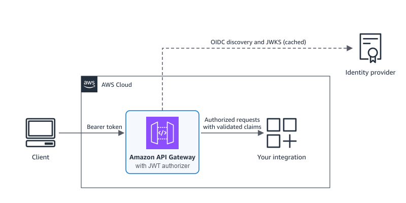
Figure 1: New architecture. API Gateway validates the token inline and forwards only authorized requests to the integration
Each request goes through the following steps:
Authorization.iss claim to a configured issuer and rejects a token from an unknown issuer before any network call.scope or scp claim.API Gateway stops processing the request at the first failed check. API Gateway returns 401 Unauthorized for a missing, malformed, expired, or untrusted token. It returns 403 Forbidden for a valid token that lacks a required scope or fails a claim rule. If API Gateway cannot reach an issuer’s key endpoint and has no cached keys, it returns a 5xx response rather than letting the request through.
In this walkthrough, you create an orders REST API in which GET /orders requires the orders:read scope and POST /orders requires orders:write.
To follow this walkthrough, you need:
/.well-known/openid-configuration.curl and jq.In your identity provider, create an API (or resource server) for the orders service with two scopes, orders:read and orders:write. Then create two machine-to-machine applications: a reporting application with only orders:read and a fulfillment application with both scopes.
Then collect the following values, shown here for three common providers.
| Value | Okta | Auth0 | Microsoft Entra ID |
ISSUER |
https://{yourOktaDomain}/oauth2/default for the default custom authorization server |
https://{yourTenant}.auth0.com/, including the trailing slash. Note that URL might include country code. |
https://login.microsoftonline.com/{tenantId}/v2.0 |
AUDIENCE |
The authorization server’s Audience, for example api://default |
The API Identifier | The application ID URI or client ID of the API app registration |
TOKEN_URL |
{ISSUER}/v1/token |
https://{yourTenant}.auth0.com/oauth/token Note that URL might include country code. |
https://login.microsoftonline.com/{tenantId}/oauth2/v2.0/token |
| Scopes | Custom scopes on the authorization server | Permissions on the API, granted to each application | See Considerations. Client credentials tokens carry app roles, not scopes. |
For the example walkthrough, set the values as environment variables (production clients can load client secrets from AWS Secrets Manager or an equivalent store).
The issuer must match the token’s iss claim exactly, including any trailing slash, so copy it from a decoded token.
Create a REST API, then describe the authorizer in a file that lists the trusted issuers, the audiences accepted from each, and the signing algorithms you configure on your issuer:
When you create or update the authorizer, API Gateway reads each issuer’s discovery document and checks that its issuer value matches. If your provider signs with an elliptic curve key, add ES256 or another supported algorithm to defaultAlgorithms. Keep jwt-config.json for step 7.
Create the /orders resource and two methods that share the authorizer but require different scopes. A mock integration returns the issuer and subject from the validated token:
Deploy the API to a stage named test and record the invoke URL:
Call the API without a token:
The request returns 401, because API Gateway rejects it before the integration runs.
Next, use a token for the reporting application, which has only orders:read, to create an order. The get_token helper sends an OAuth 2.0 client credentials request:
The request returns 403. The token is valid, but POST /orders requires orders:write.
Read orders with the reporting token, then request a token for the fulfillment application and create an order:
Both calls return 200 with the issuer and subject that the integration received:
An authorizer can trust up to 10 issuers, for example while you migrate between identity providers. In this step, you add a Cognito user pool to the same authorizer.
Create a user pool, a domain for its token endpoint, a resource server with the two scopes, and one machine-to-machine client:
Add the user pool to jwt-config.json and send the full file back, because an update replaces the whole configuration. Cognito access tokens carry the app client ID in client_id rather than aud, so use the client ID as the audience:
The following screenshot shows the updated authorizer in the API Gateway console, with the key set that API Gateway resolved for each issuer.
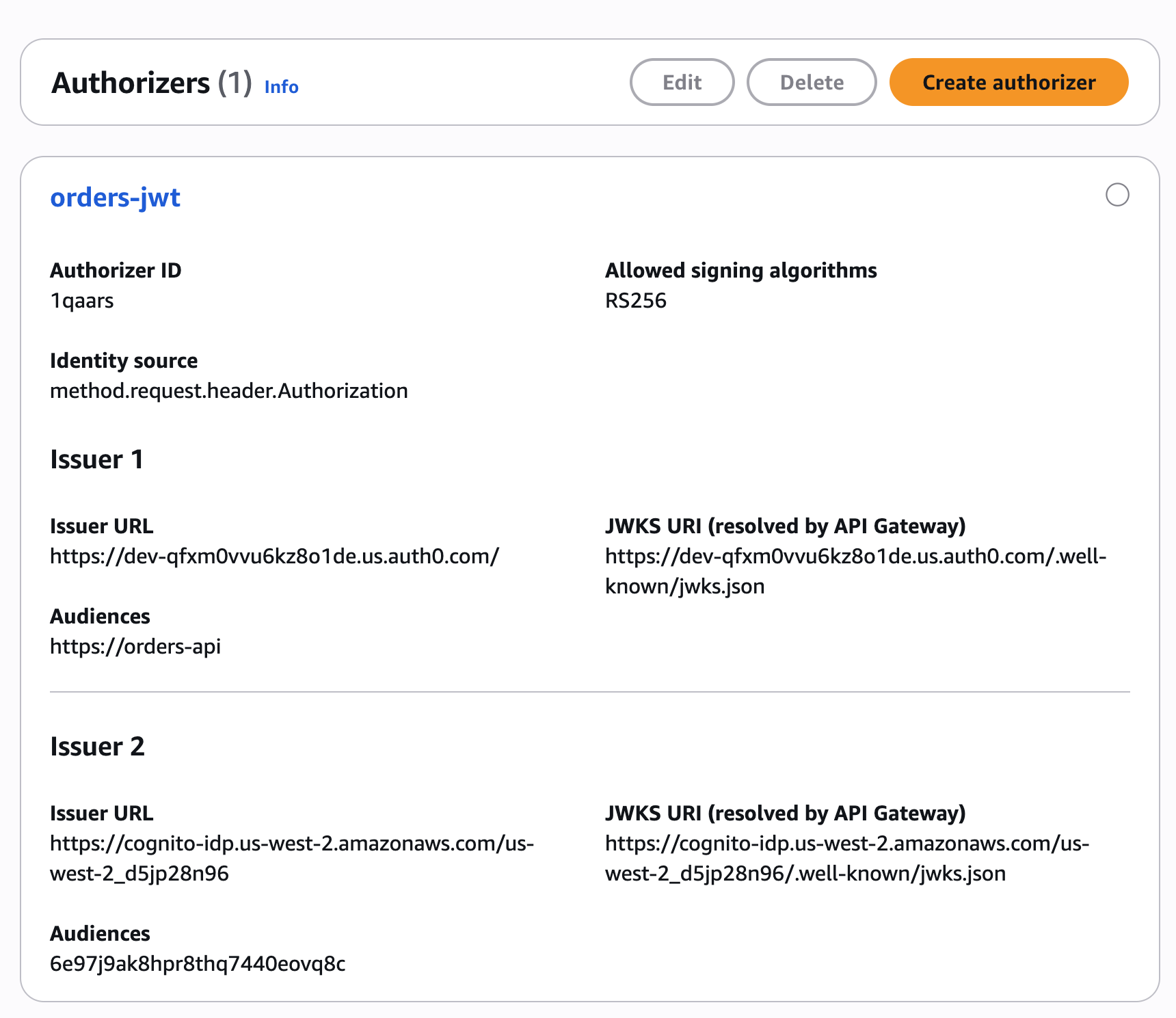
Figure 2: JWT authorizer with two trusted issuers
If you no longer have the jwt-config.json file, rebuild it from get-authorizer and remove the jwksUri fields, because API Gateway rejects an update that includes them:
Cognito names scopes {resource server}/{scope}, so its token carries orders/orders:read rather than orders:read. Add that form to GET /orders, then redeploy, because authorizer and method changes take effect only in a new deployment:
The request returns 200 with the Cognito issuer, and tokens from your original provider keep working. For Cognito issuers, a method with scopes accepts only access tokens and a method without scopes accepts only ID tokens. Give each method that client credentials callers use at least one scope.
To finish a migration, remove the retired issuer from jwt-config.json, send the same replace operation (using aws apigateway update-authorizer --patch-operations command), and redeploy.
To accept only tokens whose department claim equals eng, add a claim rule to the issuer entry. Matching is exact and case-sensitive, and API Gateway returns a 403 for other tokens:
In AWS CloudFormation, the AWS::ApiGateway::Authorizer resource has a JwtConfiguration property that mirrors the API, and methods set AuthorizationType: JWT and AuthorizationScopes:
In OpenAPI 3.0 and Swagger 2.0 definitions, use the x-amazon-apigateway-authorizer extension with type: jwt:
You can also convert an existing Lambda or Cognito authorizer in place with one update-authorizer command that changes /type, replaces /jwtConfiguration, and clears the old type’s fields. Clear Lambda fields with a replace that has no value, and remove each Cognito provider ARN with remove. Then switch each method that uses the authorizer to authorizationType: JWT, add its scopes, and redeploy.
API Gateway passes every JWT claim to your backend as JSON as it appeared in the token. Strings stay quoted and escaped, numbers stay numbers, and arrays and objects stay intact, so your backend never has to guess what was sent. Mapping templates read validated claims as $context.authorizer.claims.name, as with Cognito authorizers, and Lambda proxy integrations receive them in event.requestContext.authorizer.claims.
HTTP proxy integrations don’t forward claims automatically, so map the ones you need to headers, for example integration.request.header.x-caller to context.authorizer.claims.sub.
When API Gateway rejects a request, the response body is Unauthorized or The incoming token has expired for a 401, and Access Denied for a 403. A WWW-Authenticate header that follows RFC 6750 carries the details, such as the failed check or, for a missing scope, the scopes the method accepts.
With execution logging on, API Gateway logs a claims summary for each request, without the raw token. Data trace logging masks the Authorization header but not custom headers, so if your identity source is a header such as X-Token, keep data trace logging off for that stage.
To test an authorizer before you deploy, choose Test authorizer on the authorizer page or run test-invoke-authorizer. The test skips method scopes and accepts Cognito identity tokens, so call the deployed method to test scopes.
Before you add a JWT authorizer, consider the following:
alg: none tokens. The token header must carry a kid, which some providers omit by default.exp, nbf, and iat.scope or scp claim carries one of the method’s scopes. Microsoft Entra ID client credentials tokens carry permissions in roles instead, so use a dedicated audience per caller or a Lambda authorizer for role checks.To avoid incurring future charges, delete the resources you created:
In your identity provider, delete the two applications and the orders API or resource server if you no longer need them.
With JWT authorizers, you can validate tokens from OIDC-compatible identity providers in API Gateway REST APIs without a function in the request path. In this post, you built an API that accepted machine-to-machine tokens from your own provider, enforced separate read and write scopes, and added a Cognito user pool as a second issuer. Lambda authorizers remain the right tool for custom authorization logic. For token validation alone, we recommend the JWT authorizer.
JWT authorizers for REST APIs are available in all commercial AWS Regions, the AWS GovCloud (US) Regions, and the China Regions. To get started, refer to Controlling access to a REST API using JWT authorizers in the Amazon API Gateway Developer Guide. To learn more about serverless architectures, visit Serverless Land.
Post Syndicated from Kevin Fernandez original https://aws.amazon.com/blogs/big-data/how-veeva-scaled-big-data-with-amazon-emr-on-eks/
With biopharma commercial teams facing increasingly complex big data challenges, Veeva used Amazon EMR on EKS to increase speed and efficiency in delivering performance data to biopharma customers, supporting insight generation to find and treat more patients. Therapies designated as “orphan” in the United States that treat rare diseases affecting fewer than 200,000 Americans made up half of U.S. novel drug approvals in 2025, and the continuing shift toward developing therapies for rare and complex disease states only amplifies the need for scalable analytics infrastructure.
Veeva Systems, a leader in cloud-based software for the global life sciences industry, addresses this changing data landscape with Veeva Compass and the Compass Data Network. Compass unifies prescriptions, in-office procedures, and diagnoses into a suite of data products customers use to segment economies with greater precision, prioritize the right healthcare providers, and bring the right therapies to more patients, faster.
Veeva is continuously evaluating and adding new data partners to the Compass network, using both closed and open sources to fill the gaps left by traditional patient data products and meet the biopharma industry’s current and future data needs. To support this ever-growing network, the company undertook an ambitious architecture transformation with Amazon EMR on EKS. Veeva Compass uses faster, more efficient compute to deliver data from suppliers to customers within hours while drastically increasing efficiency by accelerating analytics and supporting AI workflows. This system flags new patient and healthcare provider (HCP) events earlier so that medical reps can engage with healthcare providers at the right time with more precise information.
This post explores the AWS analytics architecture that powers the petabyte-scale elastic big data processing Veeva Compass implemented with Amazon EMR on EKS. Specifically, it explores how Compass avoided execution slowdowns while continuing to increase data volumes to meet customer needs.
The foundation of Veeva Compass is an analytics lake that was originally designed to process hundreds of terabytes daily. Through years of consistent growth fueled by global customer expansion and the growing gap between legacy data products and industry needs, the Veeva Compass analytics lake grew. It increased support for the number of data sources and Veeva products. This resulted in an exponential growth of data volumes. With the quantity and size of batch jobs becoming more variable, Veeva decided to revisit the original Amazon EMR on Amazon Elastic Compute Cloud (Amazon EC2) architecture.
The batch job variability challenges manifested in a few important ways. Whenever Spark executors ran out of memory, the shuffle stages in Spark were unable to compensate, and executor tasks would spill to disk. This would add hours to overall job execution time with executors relying on disk storage to complete their tasks. A significant portion of the analytics budget was allocated to several provisioned Amazon EMR clusters that were idle during the afternoon waiting for the next series of job runs. To better use these clusters, Veeva distributed jobs across resources. But that led to noisy neighbor challenges where one team’s large join operation would monopolize the cluster and block another team’s service level agreement (SLA)-critical pipeline.
Veeva needed a more scalable solution that could scale out to hundreds of Spark executors in minutes when jobs arrived, then scale in when jobs complete, delivering both performance and cost efficiency. Veeva needed to rethink how it provisioned compute resources and managed Spark workloads.
Let’s explore how Veeva used Amazon EMR on EKS with Karpenter to scale its analytics capabilities and reduce Spark run times. Amazon EMR on EKS runs each Spark application as an ephemeral job inside Kubernetes, decoupling compute from storage. Data lives in Amazon Simple Storage Service (Amazon S3), durable and accessible. Spark executors run as pods that are created and terminated with each job. With Amazon EMR on EKS, Veeva is no longer dependent on always-on clusters and consumes compute only when needed.
The diversity of data types in the analytics workloads requires fine-grained control to provision the optimal compute nodes for each job. Veeva’s original cluster design relied on pre-configured node groups, where you define instance types and sizes upfront. This approach worked for other Veeva workload profiles, but Spark workloads are different. One job might need memory-optimized instances for wide joins, while another needs compute-optimized nodes for CPU-intensive transformations.
To address this challenge, Veeva added real-time EC2 instance type provisioning using Karpenter. For example, a Spark job might request 800 executors with 16 GB memory and 4 cores each. Karpenter reacts to pending pod requests in 60–90 seconds, analyzes the requirements, selects optimal instance types from across over 20 families, and launches nodes. When the job is complete, those nodes terminate within minutes. Karpenter also handles bin-packing, which is a placement strategy where pods are consolidated into fewer EKS nodes to optimize cost and improve resource utilization.
Veeva’s analytics architecture follows a medallion data design pattern. This pattern progressively refines data in stages: bronze (raw), silver (cleaned), and gold (aggregated) layers within the same storage system.
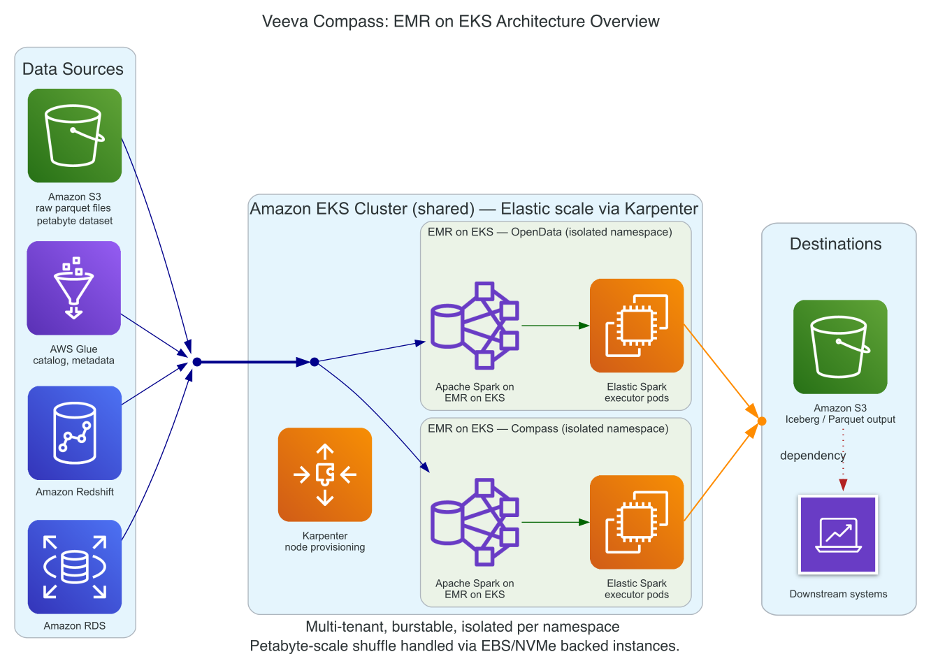
Figure 1: Amazon EMR on EKS architecture spanning the storage, compute, orchestration, and query layers
The architecture comprises four layers:
This separation of concerns delivers the elasticity required for petabyte-scale operations.
Veeva selected three distinct node profiles optimized for different Spark workload characteristics:
Driver nodes: Spark drivers and Airflow workers run on On-Demand Instances for reliability. Drivers coordinate job execution and can’t tolerate interruptions because of Spot instance reclamations. These nodes run continuously but represent less than 5 percent of total compute cost.
Executor nodes: General Extract, Transform, Load (ETL) and memory-intensive joins run on approximately 70 percent Spot Instances. Karpenter spreads across multiple instance families to maximize Spot availability. When interruptions occur, Spark’s checkpointing and Adaptive Query Execution handle recovery automatically.
Shuffle-heavy nodes: Workloads with high shuffle I/O run on NVMe-backed instances. The local SSD storage improves performance when executors spill to disk during wide joins. These run at approximately 50 percent Spot because the NVMe instance families have slightly lower Spot availability.
With the compute and orchestration layers optimized, Veeva turned its attention to improving the partition strategy, data layout, and Spark configuration.
Partition strategy: Veeva’s data is partitioned by date (YYYY-MM-DD) plus a high-cardinality dimension like region or customer segment. This simplifies partition pruning while avoiding the small-file problems that degrade query performance. Target file size is around 256–512 MB per Parquet file. Nightly compaction jobs use Delta Lake’s OPTIMIZE command with Z-ordering on frequently filtered columns, which improved query performance by 3–5x.
Shuffle and query tuning: Using Adaptive Query Execution (AQE) as a query optimization capability transformed Veeva’s most problematic Spark workload. AQE allows Spark to dynamically adjust the query plan based on runtime statistics rather than relying on static estimates. To enable these dynamic adjustments, enable AQE, configure initial partition counts for wide joins, handle data skew automatically, and enable speculative execution to recover from stragglers.
Additionally, Veeva caches some of the dimension tables in memory to avoid repeated reads from S3. For jobs that reference the same lookup tables multiple times, this optimization reduced runtime by 20–30 percent.
The combination of proper partitioning, continuous compaction, and AQE tuning reduced the skewed join stage run time from 7 hours to 55 minutes.
An observability architecture that monitors the entire stack and delivers operational insights is essential for maintaining SLAs and troubleshooting performance issues before they impact production pipelines.
The observability stack has four layers:
To help proactively identify bottlenecks before they cascade into SLA violations, Veeva configured critical alerts such as pending pods exceeding thresholds indicating capacity constraints, high shuffle-spill ratios signaling memory pressure, and excessive repartitioning indicating significant data skew.
Datasets that include prescription and claims data require robust security controls. Veeva’s architecture follows AWS best practices for least-privilege access and strict tenant isolation.
IAM Roles for Service Accounts (IRSA) provide each Spark job with temporary credentials scoped to specific S3 prefixes and AWS Lake Formation permissions. Jobs can read from bronze and silver zones but only write to their designated output paths. Using Kubernetes namespaces with taints and tolerations clearly defines workload placement. Each team operates in their own namespace with dedicated service accounts and resource quotas.
Encryption is enforced at rest with AWS Key Management Service (AWS KMS) and in transit using TLS. Amazon S3 uses customer-managed keys to encrypt all data. Spark shuffle data is encrypted using Spark’s built-in encryption. Lineage and auditing through AWS Lake Formation and OpenLineage track data transformations across the entire pipeline.
The migration from Amazon EMR on EC2 to Amazon EMR on EKS with Karpenter produced measurable improvements across every key metric:
| Metric | Amazon EMR on EC2 | Amazon EMR on EKS + Karpenter | Improvement |
| Bronze→Silver ETL (1 PB) | 9h 12m | 4h 07m | 55% faster |
| Daily 20 TB compaction | 3h 40m | 1h 55m | 48% faster |
| Scale-out 40→520 nodes | 18 min | 5m 42s | 68% faster |
| Idle EC2 cost/month | $42,000.00 | $0.00 | 100% reduction |
| Spot instance share | 0% | ~70% | ~63% cost savings |
| Bin-packing failures | Frequent | Near-zero | — |
The largest improvement came from scale-to-zero capability. The previous Amazon EMR cluster design ran 24/7 to avoid the 15–20-minute startup time, costing $42,000 monthly in idle compute. With Karpenter, nodes launch in under 6 minutes and terminate automatically, alleviating idle costs. This reduced launch time matters when you have SLA-critical pipelines that need to start processing immediately. For the largest bronze-to-silver ETL job processing approximately 1 PB of data, Karpenter scaled the cluster from 40 to 520 nodes in 5 minutes 42 seconds. It then spun everything down minutes after completion. That level of elasticity is difficult to achieve with traditional automated scaling approaches. By diversifying across over 20 Spot instance types, Karpenter achieves higher Spot availability and lower interruption rates. The executor fleet runs approximately 70 percent Spot, delivering approximately 63 percent cost savings compared to On-Demand pricing.
For Veeva Compass’s business, the speed improvements are as impactful as the cost savings. Several of their most common customer use cases are highly dependent on data delivery speed. For example, medical field reps at a biopharma company rely on alerts from patient data to guide their engagement strategies day to day. The faster Veeva can deliver a new diagnosis or procedure to a customer, the faster that customer’s field team can act.
After a year of operating petabyte-scale analytics on Amazon EMR on EKS, here are the lessons that delivered the most value:
Veeva Compass’s journey from Amazon EMR on EC2 to Amazon EMR on EKS with Karpenter demonstrates how modern cloud-native architectures can transform petabyte-scale analytics workloads. By embracing ephemeral compute, intelligent autoscaling, and continuous optimization, Veeva achieved measurable improvements in both performance and cost efficiency. They reduced critical ETL runtimes by over 50 percent while alleviating $42,000 in monthly idle compute costs.
These cost and performance improvements are important for Veeva Compass’s business practice. The ability to quickly serve large amounts of data to biopharma commercial teams enables faster and more precise analytics, especially as biopharma companies continue to drive increased data demand by exploring AI use cases. These improvements help Veeva Compass customers act with speed and precision to quickly deliver the right therapies to patients in need.
If you’re facing similar challenges with growing data volumes and complex Spark workloads, consider exploring Amazon EMR on EKS and Karpenter as a foundation for elastic, cost-effective big data processing. To learn more about building scalable analytics on AWS, visit the Amazon EMR documentation and explore Karpenter best practices.
Post Syndicated from Rapid7 original https://www.rapid7.com/blog/post/etr-cve-2026-114938-reported-critical-pre-authentication-remote-code-execution-java-17
On November 17, 2026, public reports described CVE-2026-114938 as a memory corruption vulnerability in Java 17 and above that could allow a remote attacker to execute code without authentication. The reported severity is Critical, with a CVSSv4 score of 9.2. These CVE-specific details remain preliminary, pending confirmation in Oracle or OpenJDK advisories.
Rapid7 is actively monitoring the situation and will update this blog as new information arrives.
For the latest vendor release information, refer to Oracle’s November security update notice and OpenJDK’s vulnerability advisories.
Exposure Command, Vulnerability Management, and Nexpose customers can assess exposure to CVE-2026-114938 with an authenticated vulnerability check available in the November 17 content release (1.1.4115).
November 17, 2026: Initial publication.
Post Syndicated from Lakshmi Kumkala original https://aws.amazon.com/blogs/devops/secure-mcp-integrations-for-aws-devops-agent-with-amazon-bedrock-agentcore/
When the agent can’t reach data you need during an incident investigation, you extend it with new tools. You also manage the security and observability overhead of each tool you add. As you connect more Model Context Protocol (MCP) tools to AWS DevOps Agent, your security team ends up tracking a separate authentication scheme, credential rotation schedule, and audit or revocation procedure for each one. This post shows how to extend AWS DevOps Agent with MCP tools securely, using Amazon Bedrock AgentCore, so that new tools can inherit consistent security, access control, private connectivity, and observability.
AWS DevOps Agent is an AI-powered, always-available operations teammate that autonomously investigates incidents, identifies root causes, and prevents future issues across AWS, multicloud, and on-premises environments. It correlates Amazon CloudWatch metrics, logs, traces, and deployment history to produce root-cause analyses in minutes instead of hours. In Announcing General Availability of AWS DevOps Agent, AWS reported results from customers and partners who used AWS DevOps Agent in preview. They saw up to 75 percent lower mean time to resolution (MTTR), 80 percent faster investigations, and 94 percent root-cause accuracy.
By default, AWS DevOps Agent integrates with a broad set of observability, source control, continuous integration and continuous delivery (CI/CD), ticketing, and collaboration services. Real-world operational environments often extend further: proprietary configuration management databases (CMDBs), internal runbook APIs, application logs in OpenSearch, custom deployment tracking systems, or self-hosted tools behind private networks. When you need data from a source without a native integration, you can use MCP tools to give the agent a standardized way to call external services during an investigation.
You will learn when an MCP tool is the right answer, where to host it, how to connect it to AWS DevOps Agent, and how AgentCore Gateway, a capability of Amazon Bedrock AgentCore, provides a unified management layer for security, policy, and observability.
Before examining tool infrastructure, it helps to see where MCP tools enter the picture. When your Amazon CloudWatch alarms, ServiceNow tickets, or PagerDuty alerts trigger an incident, AWS DevOps Agent begins an autonomous investigation. The following diagram shows where MCP tools extend that investigation beyond the agent’s native integrations.
Figure 1: MCP tools extend the investigation reach of AWS DevOps Agent beyond its native and built-in integrations
These tools can connect to internal operational tools, third-party platforms, on-premises systems, or any custom data source you want to expose to an agent space. AWS DevOps Agent provides logging and the ability to disconnect any MCP server from the console, but you configure authentication, rotate credentials, and maintain the audit trail for each server. As the number of MCP servers grows, managing them independently creates compounding overhead: separate credential lifecycles, no cross-tool policy enforcement, and no unified view for observability across all tools.
AgentCore Gateway helps reduce this per-tool overhead. The agent connects to one endpoint, and tools behind that endpoint share the same security, policy, and observability configuration.
For more on triggering investigations automatically, see Trigger DevOps Agent from CloudWatch Alarms & Amazon EventBridge and Automating DevOps Agent from Incident Detection and Response alarms.
Use this decision framework to choose between a native integration, an existing MCP server, and building a custom MCP server when you need a new data source or workflow.
Figure 2: Decision framework for extending AWS DevOps Agent: native integration, existing MCP server, or custom MCP server
Start with what AWS DevOps Agent already covers. Before building anything, check the native capability list on the Capability Providers page. These integrations need no custom server to build or host. AWS DevOps Agent Tools catalogs additional MCP servers built for use with the agent. It is also worth browsing the AWS DevOps Agent ACP/MCP samples repository for reference implementations, and awslabs/mcp for AWS-published open source MCP servers such as the Amazon Managed Service for Prometheus MCP server and the Amazon Elastic Kubernetes Service (Amazon EKS) MCP server.
If a source is not natively covered, check whether a vendor already publishes an MCP server before building your own. Many do. For example, Atlassian’s Rovo MCP Server covers Jira, Confluence, Jira Service Management, and Bitbucket, and vendors such as Datadog and PagerDuty publish official servers.
Build a custom MCP tool when your source does not fall into any of these categories. The most common scenarios are:
AgentCore Gateway also provides one-click integrations for tools such as Jira, Salesforce, Slack, Asana, and Zendesk, as well as native support for Amazon Bedrock Knowledge Bases as a Gateway target. If your tool is available as a one-click target, you can skip building a custom MCP server and register it directly on the Gateway, which you then connect to AWS DevOps Agent as an MCP server through the agent’s capabilities.
After you decide to build a custom MCP tool, you need to choose where it runs. The right choice depends on statefulness, latency tolerance, connection requirements, and how much infrastructure you want to manage. The following table compares the four most common hosting options.
| Hosting option | Best for | Advantages | Trade-offs |
| AWS Lambda (direct IAM invoke) | Stateless, read-heavy tools that execute quickly, such as Amazon S3 log parsers, OpenSearch query wrappers, runbook search, and internal API or ticket lookups | No infrastructure to manage, pay-per-invocation, and auto-scales to zero. AgentCore Gateway invokes Lambda directly through IAM, without needing the HTTP layer, which removes Amazon API Gateway latency for Gateway-connected tools | 15-minute execution limit, cold-start latency on first invoke, and no persistent connections |
| AWS Lambda with Amazon API Gateway | Shared tools used by multiple teams or systems, and tools that require request throttling or AWS WAF protection | All Lambda benefits, plus HTTP-level controls such as throttling, WAF protection, custom domains, and per-caller access logging | Added per-request latency, Amazon API Gateway per-request cost, and more configuration |
| Amazon Bedrock AgentCore runtime | Teams who want zero-ops MCP hosting with native multi-turn session support | No infrastructure to manage, built-in session isolation, native MCP protocol support, both stateless and stateful modes, and support for your own container image. Works with any MCP framework, including LangGraph, CrewAI, and Strands Agents | Cold-start latency when a new session starts, and less control over the underlying compute than Amazon Elastic Container Service (Amazon ECS) |
| Amazon ECS on AWS Fargate | Database query tools that maintain connection pools, and tools with expensive initialization or large in-memory caches | No cold starts, persistent connections, and full control over the runtime environment | Always-on cost even when idle, and container image management overhead |
For hosting walkthroughs, see Connect API Gateway to AgentCore Gateway with MCP for the API Gateway pattern and Deploy MCP servers in Runtime for AgentCore runtime. The AgentCore runtime released in September 2026 reduces cold starts to about two seconds at p75 regardless of container image size.
As a rule of thumb, start with Lambda for most read-only tools, move to AgentCore runtime, a capability of Amazon Bedrock AgentCore, when you need multi-turn sessions or zero-ops hosting, and use Amazon ECS when you need persistent connections or large in-memory state.
There are two ways to connect MCP servers to AWS DevOps Agent. The right choice depends on how many tools you have, whether tool access needs to be consistent across multiple accounts, and whether you need central policy enforcement. The following diagram compares a direct per-account connection with a single connection through AgentCore Gateway.
Figure 3: Connecting MCP servers to AWS DevOps Agent: direct connection compared to AgentCore Gateway
With a direct connection, you register each MCP server at the AWS account level from the Capability Providers page. To register a server:
Your MCP server must implement the streamable HTTP transport protocol and support one of the following authentication methods:
AWS DevOps Agent supports private connections natively. When you register an MCP server, select Connect to endpoint using private connection and choose or create a private connection. AWS DevOps Agent uses Amazon VPC Lattice to route traffic to your private endpoint entirely over the AWS network, with no public endpoint needed. Private connections work with any integration that needs to reach a private endpoint, including self-hosted Grafana or Splunk instances and source control systems such as GitHub Enterprise Server and GitLab Self-Managed. For a detailed walkthrough, see Securely connect AWS DevOps Agent to private services in your VPCs.
When you connect an MCP server, you classify each of its tools as read-only, mutating, or destructive. The console prompts you for each tool, and API or CLI registrations set this with toolDetails. Read-only tools run without operator approval. Mutating tools are available only after you enable directed actions on the agent space, and each call requires operator approval in chat. AWS DevOps Agent does not invoke tools classified as destructive. If you register a server through the API or CLI without classifying its tools, every tool defaults to read-only, so classify any tool that can change state. For more information, see Working with directed actions.
Custom MCP servers can introduce additional prompt-injection risk. Allow only the tools each agent space needs, prefer read-only tools, and give each server’s credentials read-only access. For more information, see the security considerations in Connecting MCP Servers.
AgentCore Gateway is a fully managed service that provides a single, secure entry point for agentic traffic, connecting agents to tools, to other agents, and to models. Instead of registering each MCP server independently in the AWS DevOps Agent account, you register all of them as targets on the Gateway. AWS DevOps Agent registers the Gateway URL once at the account level, and all tools from all registered targets become available through that single registration.
Gateway also consolidates authentication. AWS DevOps Agent connects to a single Gateway endpoint with AWS SigV4. It signs requests with either a dedicated IAM role or, if you register without one, the IAM role of the AWS account associated with the agent space. Grant that role bedrock-agentcore:InvokeGateway, scoped to the Gateway ARN. You still configure per-target credentials on the Gateway, because each backend MCP server has its own authentication. But the Gateway manages those credentials centrally, handling token refresh, secure storage, and credential lifecycle in one place rather than scattering them across individual agent space registrations.
With Policy in Amazon Bedrock AgentCore, you can enforce Cedar rules across every tool behind the Gateway with a single policy, for example blocking any tool that writes to production resources regardless of which MCP server exposes it. Because AWS DevOps Agent already refuses tools classified as destructive, Gateway policy is most valuable as an independent backstop in case someone misclassifies a tool.
Gateway also provides a unified audit trail and built-in observability automatically, with no instrumentation code and no per-target logging configuration. Amazon CloudWatch Logs records every tool call, including tool name, caller identity, request arguments, response, latency, and status, across all registered targets in one log group. AWS X-Ray provides end-to-end distributed traces across the MCP client, Gateway, and Lambda or runtime layers. The CloudWatch generative AI observability dashboard reports per-tool metrics, including invocation count, error rate, and latency percentiles (p50, p90, and p99). These metrics appear regardless of whether the tool runs on Lambda, Amazon ECS, AgentCore runtime, or a third-party server.
Gateway can also route to private MCP servers through VPC Lattice egress. If you need private connectivity together with the authentication, policy, and observability capabilities of the Gateway, register the tool as a private Gateway target. For connectivity patterns, see Private connectivity patterns for AgentCore Gateway Targets. If you only need private connectivity for a single tool without central policy, a direct private connection requires less configuration.
You can also route native MCP integrations through Gateway. Some AWS DevOps Agent native capabilities, such as the Grafana integration, connect to external MCP servers (Grafana’s own MCP server, in this case). If you want unified policy enforcement, observability, and authentication across both your native MCP-based integrations and your custom MCP servers, you can route them through AgentCore Gateway as well. This gives you a single control plane regardless of whether the tool came from the Capability Providers page or a custom registration.
For more on extending Gateway with MCP servers, see Extending MCP support for AgentCore Gateway and Transform your MCP architecture: Unite MCP servers through AgentCore Gateway.
Use a direct connection when you have one or two MCP servers in a single AWS account, when each agent space configures its own tool set manually, and when you do not need cross-cutting policy enforcement. Choose AgentCore Gateway when you have multiple MCP servers and want to manage them through a single registration, when agent spaces across multiple AWS accounts need to share the same tools, when you want one authentication configuration, when you need Cedar policy enforcement across all tools, or when you want a unified audit trail and built-in observability. For full instructions, see Connecting MCP Servers in the AWS DevOps Agent User Guide.
This table maps common scenarios to the recommended connection approach.
| Scenario | Recommended approach |
| One or two MCP servers, single account | Direct connection |
| Multiple MCP servers, single registration preferred | AgentCore Gateway |
| Agent spaces across multiple AWS accounts sharing the same tools | AgentCore Gateway |
| Private VPC tool, no central policy needed | Direct connection with DevOps Agent private connection |
| Private VPC tool with Cedar policy or unified auth | Gateway with VPC Lattice target |
| Cedar policy enforcement across all tools | AgentCore Gateway |
| Unified audit trail across all MCP servers | AgentCore Gateway |
Beyond choosing a connection path, Gateway gives you finer control over which tools an agent space can reach.
Keep the per-space tool ceiling in mind as you scope access: a single agent space can have at most 500 MCP tools on the allowlist across all of its MCP servers, and this limit is not adjustable. Scoping each space to only the tools it needs keeps you well under that ceiling. For the full list of limits, see AWS DevOps Agent quotas.
When AWS DevOps Agent connects to an MCP server, its tools appear on the agent space console, where an admin selects which tools to allow and classifies each one as read-only, mutating, or destructive. This workflow exists with or without Gateway.
Gateway adds a mechanism on top: separate targets per tool category. Register read-only tools and write or destructive tools as separate Gateway targets, then associate AWS DevOps Agent with only the read-only target. The write tools don’t appear in that agent space, because they are not in the target. For how to register targets, see Add targets to an existing AgentCore Gateway.
For example, if an MCP server exposes list_runbooks, get_runbook, search_runbooks, upload_runbook, and delete_runbook, register a target named readonly-runbook-tools with only the first three. Connect the production agent space to the readonly-runbook-tools target, and connect development and staging agent spaces to a target that exposes all five tools.
Even when tools are visible and enabled in an agent space, Gateway policy, which uses Cedar, can block execution. This is the enforcement boundary below the admin workflow, and it holds regardless of what an admin configures on the console, which helps guard against configuration mistakes. For more on Cedar policy patterns, see Secure AI agents with Policy in Amazon Bedrock AgentCore.
AWS DevOps Agent covers a broad set of AWS services and third-party tools by default. When investigations need to reach further, into OpenSearch, internal runbook APIs, proprietary CMDBs, or tools in private VPCs, MCP tools extend that reach.
For one or two tools in a single account, a direct connection with account-level registration is sufficient. The picture changes when MCP servers multiply, when agent spaces span multiple AWS accounts, or when security teams need consistent enforcement and a unified audit trail. AgentCore Gateway collapses that to one registration per account pointing to a single Gateway URL. You configure authentication once, enforce Cedar policies consistently, get built-in CloudWatch observability across your tools, and revoke access in one place instead of across each tool registration.
For more on what AWS DevOps Agent can do by default, see Announcing General Availability of AWS DevOps Agent, AWS DevOps Agent features, and Native Capabilities.
To try this pattern, register one read-only MCP server as an AgentCore Gateway target, connect the Gateway to a non-production agent space, and classify each tool before you enable it. The following resources cover each step.
| What | Link |
| AWS DevOps Agent overview | Product page · User Guide |
| Connecting MCP servers to AWS DevOps Agent | User Guide – Connecting MCP Servers |
| AgentCore Gateway | Developer Guide – Gateway · Getting started |
| Cedar policy for Gateway | Understanding Cedar · Core concepts · Schema constraints |
| AgentCore runtime (MCP hosting) | Deploy MCP servers in Runtime |
| Private connectivity | VPC Lattice egress · Private endpoints · DevOps Agent private connections |
| Observability | Service-provided observability · Observability overview |
| Gateway authentication | Inbound auth setup · Cognito as IdP |
| Related blog posts | Transform your MCP architecture with Gateway · Connect API Gateway to AgentCore Gateway · Why AgentCore chose Cedar |
| MCP/ACP samples | DevOps Agent ACP/MCP samples |
| Samples | DevOps Agent + CloudWatch sample |
Post Syndicated from Connor Peet original https://github.blog/engineering/engineering-principles/building-the-agent-host-protocol-for-sessions-that-continue-across-devices/
Models are now good enough to work for hours or even days on their own. You don’t have to watch over every thing they do, but you still need to be able to check in, no matter where you are. An agent can’t live only inside one application. The work should continue even If you close a window or switch devices.
In GitHub Copilot you can start an agent session in one place and pick it up in another. This session continuity runs on the Agent Host Protocol (AHP), an open standard built first in VS Code and adopted across GitHub. Here’s how it works, what we learned building it, and how you can use it to bring your agents into your own apps and workflows.
GitHub Copilot was first built in VS Code as an extension that bundled its own harness. This gave you access to your agents in VS Code, but it tied their lifetime to the editor. Extensions are attached to a single VS Code window. Close that window, and the agent is gone. Update VS Code, and every agent stops as the application restarts. Connect to a remote machine, and you get an entirely new extension host commit-locked against the version of the VS Code workbench you have.
At the same time, the Copilot app was being developed, alongside the existing GitHub mobile apps for iOS and Android. Each product was doing its own distinct integration with cloud-based agents to work towards delivering session continuity.
Each of these integrations solved the problem for one product, but developers also still want to be able to pull their agents into their own workflows–whether that’s an editor, a terminal, a phone, or a tool they built themselves–and they can’t do that if every client needs its own one-off integration. That’s why developers needed a protocol: a standard, independently versioned language across versions of VS Code, the GitHub Copilot app, mobile apps, and any other client that might host an agent. A shared protocol means every client sees the same agents, history, and state without bespoke integrations, and you aren’t tied to one app’s idea of what an agent session is.
The protocol needed to allow multiple clients to interact with the same set of agents seamlessly. Start a session in the cloud from your phone, for example, then continue it from your laptop. It should tolerate network interruptions, reconnections, and concurrent client mutations. And it needed to be full-featured enough for you to do real work from each of your clients.
At the same time, the protocol needed to stay out of agent behavior. Unlike the domains that produced the Language Server Protocol and Debug Adapter Protocol, the world of agents is evolving quickly. That’s why AHP avoids encoding how agents work, and instead focuses on how you want to interact with them.
You also need the protocol to be simple enough to implement on your own client or server. While the full feature set would necessarily be extensive, the core protocol needed to be minimal.
The result of these requirements is the Agent Host Protocol (AHP). It is oriented around URI-identified “channels”, which are the coarsest unit of functionality in the protocol. Every server must implement the root, session, and chat channels, but can also implement more channels that provide terminal support, MCP additions, or OTel reporting, for example.
Within each channel is a reducer-based state object, which drives most of the logic for clients. The server is the arbiter of the state, and each client sends a sequence of actions that either mutate the state or trigger side effects, like sending a chat message. This provides a few very nice properties. Reconnection and replay in poor network conditions are easy: a client sends all queued actions, presents the right ‘loading’ state, and waits for the server to reconcile and acknowledge the actions before confirming them. Clients and servers are straightforward to debug. And reducer-based state also plays nicely with popular UI frameworks like React.
Adopting the Agent Host Protocol in VS Code required building a new harness and agentic stack underneath it. The Copilot Chat extension, which used to provide all of VS Code’s AI and agentic capabilities, had been growing for over three years, reaching over 400,000 lines of TypeScript, not counting tests. But, as a VS Code extension, it was structured around the lifecycle of a VS Code window and depended entirely on the VS Code extension API. Neither that lifetime nor those APIs would be available in a standalone agent host process.
As we started building the Agent Host Protocol in early 2026, the Copilot SDK was also being developed, and it made sense to leverage it as the foundation for the new agentic stack. This was a big transition. It’s easy to build a harness implementation that says hello and can edit files—we were using the agent host to develop the agent host after the first couple weeks—but it’s another thing to build one that covers the long tail of features developers had come to expect from Copilot Chat.
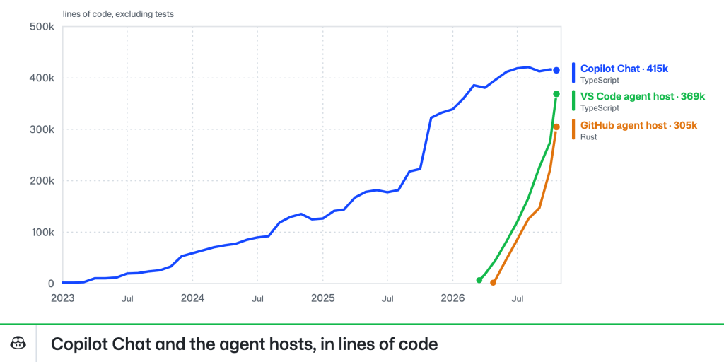
GitHub has had Copilot cloud agents for a couple of years, allowing developers to run tasks in the cloud from any device. While VS Code was quietly developing the Agent Host Protocol, GitHub was looking to expand that capability to coordinate sessions running on your own devices via the Copilot app, or in cloud sandboxes. This was exactly the N:M problem that AHP was built to solve, so adopting the same technology made perfect sense.
From the outset, the GitHub Agent Host had different requirements than VS Code’s implementation. VS Code runs the host locally and can drop its host on other compute over SSH, containers, WSL, or Dev Tunnels, and it is actually included as part of the VS Code Server bundle. The GitHub Agent Host needed to run in the cloud and across a much wider variety of infrastructure, environments, and security constraints.
Those differing requirements are why they’re separate implementations written in different languages: VS Code’s in TypeScript and GitHub’s in Rust. For now, having two agent hosts has been a good acid-test for the protocol itself. How well does it work when two entirely different teams and sets of agents implement the same protocol independently?
Pretty well, it turns out. Like MCP, the Agent Host Protocol provides escape hatches via custom methods and _metadata on objects that consumers can use for out-of-band signaling. After several months heads-down on our respective implementations, our first task as we worked toward unification was inventorying the ways each implementation had extended the protocol. Many of these extensions reasonably stay GitHub-specific, such as the GitHub Agent Host using metadata to link to project boards. In other cases, variance was a sign of a gap in the protocol; early versions, for example, could not accurately represent shell-type tool output that wasn’t backed by a PTY. And some were bad assumptions, like VS Code’s client assuming a particular structure for the session URIs it received from the agent host. A protocol with only one implementation isn’t truly portable; as we taught our clients and servers to talk to each other, AHP became portable in practice, not just in theory.
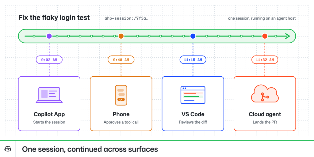
Today, the Agent Host Protocol provides that same continuity across all VS Code and GitHub surfaces. Agent sessions running locally in the GitHub Copilot app, in cloud sandboxes, and in VS Code all share the same underlying protocol. To see how it’s used, read about how you can work from anywhere with the new connected Copilot cloud experience.
AHP was designed to be easy to use in clients and servers. Agent Host Protocol libraries are available in Rust, TypeScript, Kotlin, Swift, .NET, and Go, and agents are able to build clients and servers with little prompting. I have a macropad sitting on my desk that reflects my agent’s state in real time, and others have built everything from smart watch apps to Kanban-style task management tools against the protocol. Whether you want a companion app for your own agents, a way to bring agent sessions into your team’s tools, or AHP support in your own editor or agent, the protocol is open for you to build on.
You can connect to an agent host you implement in the Copilot app (enable Experimental > Direct Connections, then go to Environments > Add Agent Host Protocol Host) and in VS Code (via Add Remote Agent Host in the Agents window). You can spawn a standalone version of VS Code’s agent host by running code agent host in your terminal, or see the endpoints for the one in your editor by running code agent endpoints, and samples can help you and your agent get started.
The Agent Host Protocol is an open standard, and questions and suggestions are welcome on GitHub.
Happy coding!
The post Building the Agent Host Protocol for sessions that continue across devices appeared first on The GitHub Blog.