Post Syndicated from Renan Dincer original https://blog.cloudflare.com/cloudflare-calls-anycast-webrtc
Following its initial announcement in September 2022, Cloudflare Calls is now in open beta and available in your Cloudflare Dashboard. Cloudflare Calls lets developers build real-time audio/video apps using WebRTC, and it abstracts away the complexity by turning the Cloudflare network into a singular SFU. In this post, we dig into how we make this possible.
WebRTC growing pains
WebRTC is the only way to send UDP traffic out of a web browser – everything else uses TCP.
As a developer, you need a UDP-based transport layer for applications demanding low latency and real-time feedback, such as audio/video conferencing and interactive gaming. This is because unlike WebSocket and other TCP-based solutions, UDP is not subject to head-of-line blocking, a frequent topic on the Cloudflare Blog.
When building a new video conferencing app, you typically start with a peer-to-peer web application using WebRTC, where clients exchange data directly. This approach is efficient for small-scale demos, but scalability issues arise as the number of participants increases. This is because the amount of data each client must transmit grows substantially, following an almost exponential increase relative to the number of participants, as each client needs to send data to n-1 other clients.
Selective Forwarding Units (SFUs) play pivotal roles in scaling WebRTC applications. An SFU functions by receiving multiple media or data flows from participants and deciding which streams should be forwarded to other participants, thus acting as a media stream routing hub. This mechanism significantly reduces bandwidth requirements and improves scalability by managing stream distribution based on network conditions and participant needs. Even though it hasn’t always been this way from when video calling on computers first became popular, SFUs are often found in the cloud, rather than home computers of clients, because of superior connectivity offered in a data center.
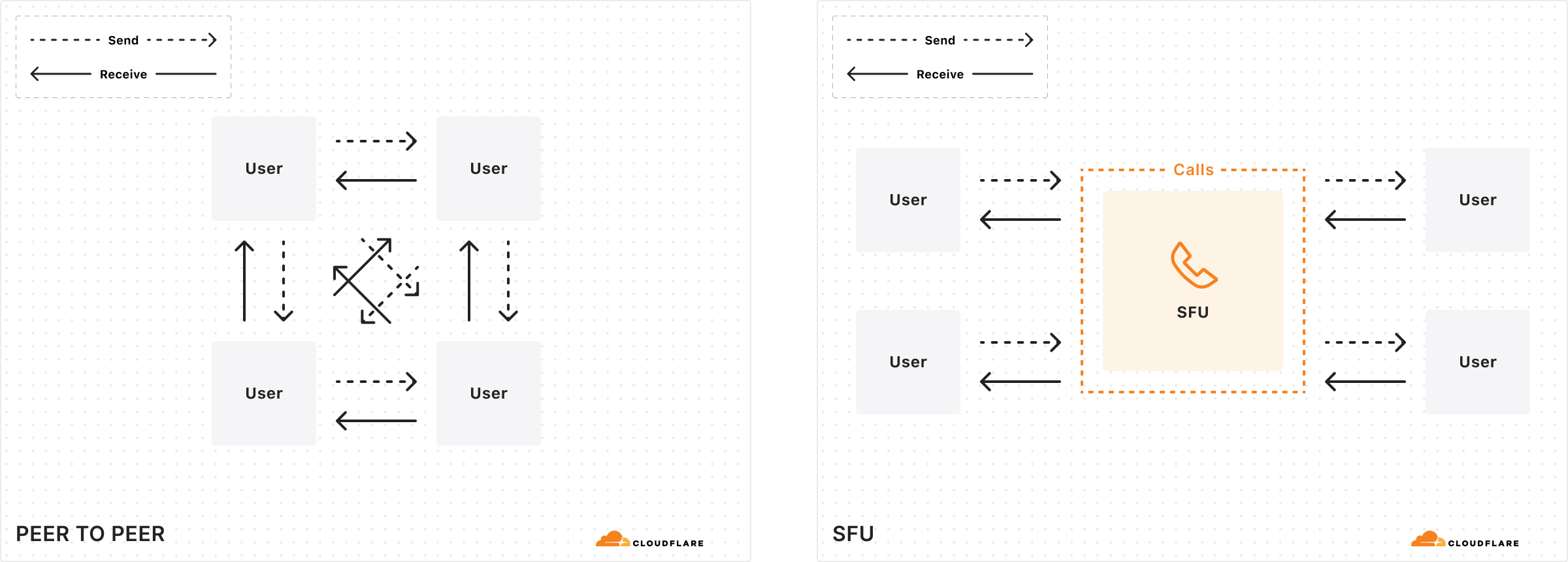
A modern audio/video application thus quickly becomes complicated with the addition of this server side element. Since all clients connect to this central SFU server, there are numerous things to consider when you’re architecting and scaling a real-time application:
- How close is the SFU server location(s) to the end user clients, how is a client assigned to a server?
- Where is the SFU hosted, and if it’s hosted in the cloud, what are the egress costs from VMs?
- How many participants can fit in a “room”? Are all participants sending and receiving data? With cameras on? Audio only?
- Some SFUs require the use of custom SDKs. Which platforms do these run on and are they compatible with the application you’re trying to build?
- Monitoring/reliability/other issues that come with running infrastructure
Some of these concerns, and the complexity of WebRTC infrastructure in general, has made the community look in different directions. However, it is clear that in 2024, WebRTC is alive and well with plenty of new and old uses. AI startups build characters that converse in real time, cars leverage WebRTC to stream live footage of their cameras to smartphones, and video conferencing tools are going strong.
WebRTC has been interesting to us for a while. Cloudflare Stream implemented WHIP and WHEP WebRTC video streaming protocols in 2022, which remain the lowest latency way to broadcast video. OBS Studio implemented WHIP broadcasting support as have a variety of software and hardware vendors alongside Cloudflare. In late 2022, we launched Cloudflare Calls in closed beta. When we blogged about it back then, we were very impressed with how WebRTC fared, and spoke to many customers about their pain points as well as creative ideas the existing browser APIs can foster. We also saw other WebRTC-based apps like Clubhouse rise in popularity and Twitter Spaces play a role in popular culture. Today, we see real-time applications of a different sort. Many AI projects have impressive demos with voice/video interactions. All of these apps are built with the same WebRTC APIs and system architectures.
We are confident that Cloudflare Calls is a new kind of WebRTC infrastructure you should try. When we set out to build Cloudflare Calls, we had a few ideas that we weren’t sure would work, but were worth trying:
- Build every WebRTC component on Anycast with a single IP address for DTLS, ICE, STUN, SRTP, SCTP, etc.
- Don’t force an SDK – WebRTC APIs by themselves are enough, and allow for the most novel uses to shine, because best developers always find ways to hit the limits of SDKs.
- Deploy in all 310+ cities Cloudflare operates in – use every Cloudflare server, not just a subset
- Exchange offer and answer over HTTP between Cloudflare and the WebRTC client. This way there is only a single PeerConnection to manage.
Now we know this is all possible, because we made it happen, and we think it’s the best experience a developer can get with pure WebRTC.
Is Cloudflare Calls a real SFU?
Cloudflare is in the business of having computers in numerous places. Historically, our core competency was operating a caching HTTP reverse proxy, and we are very good at this. With Cloudflare Calls, we asked ourselves “how can we build a large distributed system that brings together our global network to form one giant stateful system that feels like a single machine?”
When using Calls, every PeerConnection automatically connects to the closest Cloudflare data center instead of a single server. Rather than connecting every client that needs to communicate with each other to a single server, anycast spreads out connections as much as possible to minimize last mile latency sourced from your ISP between your client and Cloudflare.
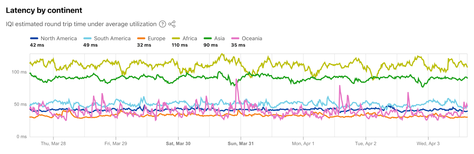
It’s good to minimize last mile latency because after the data enters Cloudflare’s control, the underlying media can be managed carefully and routed through the Cloudflare backbone. This is crucial for WebRTC applications where millisecond delays can significantly impact user experience. To give you a sense about latency between Cloudflare’s data centers and end-users, about 95% of the Internet connected population is within 50ms of a Cloudflare data center. As I write this, I am about 20ms away, but in the past, I have been lucky enough to be connected to a **great** home Wi-Fi network less than 1ms away in Manhattan. “But you are just one user!” you might be thinking, so here is a chart from Cloudflare Radar showing recent global latency measurements:
This setup allows more opportunities for packets lost to be replied with retransmissions closer to users, more opportunities for bandwidth adjustments.
Eliminating SFU region selection
A traditional challenge in WebRTC infrastructure involves the manual selection of Selective Forwarding Units (SFUs) based on geographic location to minimize latency. Some systems solve this problem by selecting a location for the SFU after the first user joins the “room”. This makes routing inefficient when the rest of the participants in the conversation are clustered elsewhere. The anycast architecture of Calls eliminates this issue. When a client initiates a connection, BGP dynamically determines the closest data center. Each selected server only becomes responsible for the PeerConnection of the clients closest to it.
One might see this is actually a simpler way of managing servers, as there is no need to maintain a layer of WebRTC load balancing for traffic or CPU capacity between servers. However, anycast has its own challenges, and we couldn’t take a laissez-faire approach.
Steps to establishing a PeerConnection
One of the challenging parts in assigning a server to a client PeerConnection is supporting dual stack networking for backwards compatibility with clients that only support the old version of the Internet Protocol, IPv4.
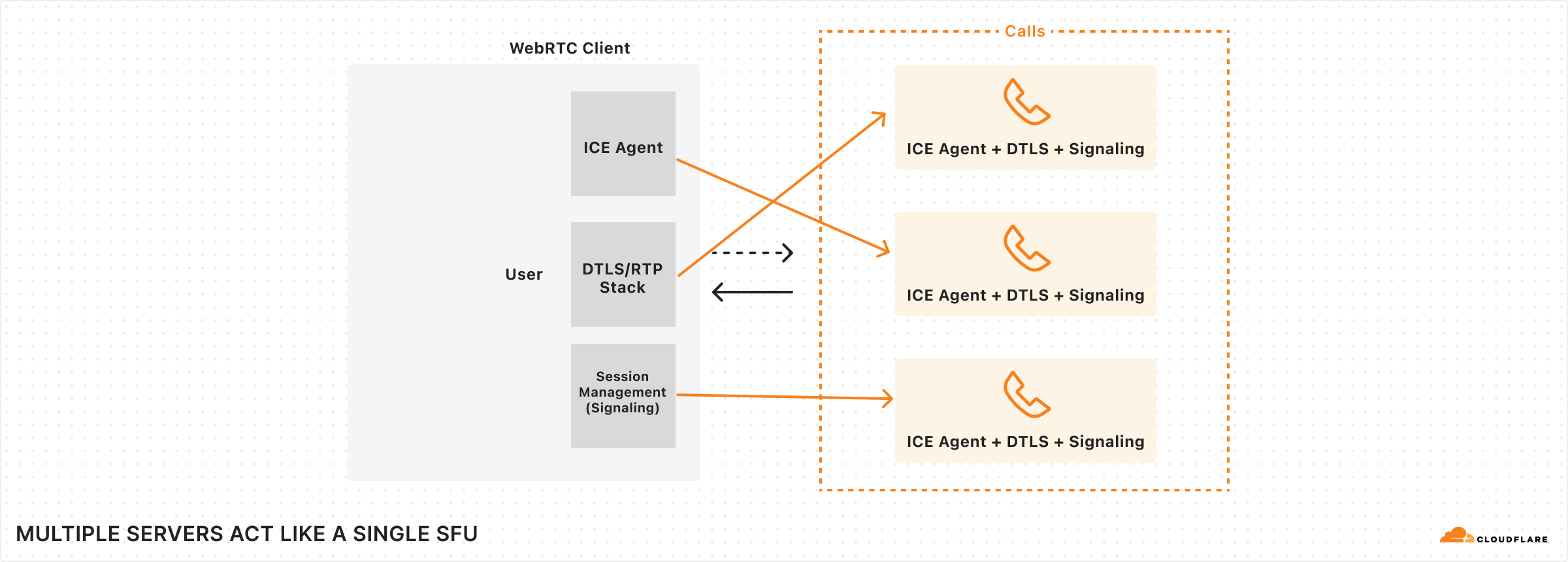
Cloudflare Calls uses a single IP address per protocol, and our L4 load balancer directs packets to a single server per client by using the 4-tuple {client IP, client port, destination IP, destination port} hashing. This means that every ICE connectivity check packet arrives at different servers: one for IPv4 and one for IPv6.
ICE is not the only protocol used for WebRTC; there is also STUN and TURN for connectivity establishment. Actual media bits are encrypted using DTLS, which carries most of the data during a session.
DTLS packets don’t have any identifiers in them that would indicate they belong to a specific connection (unlike QUIC’s connection ID field), so every server should be able to handle DTLS packets and get the necessary certificates to be able to decrypt them for processing. DTLS encryption is negotiated at the SDP layer using the HTTPS API.
The HTTPS API for Calls also lands on a different server than DTLS and ICE connectivity checks. Since DTLS packets need information from the SDP exchanged using the HTTPS API, and ICE connectivity checks depend on the HTTPS API for userFragment and password fields in the connectivity check packets, it would be very useful for all of these to be available in one server. Yet in our setup, they’re not.
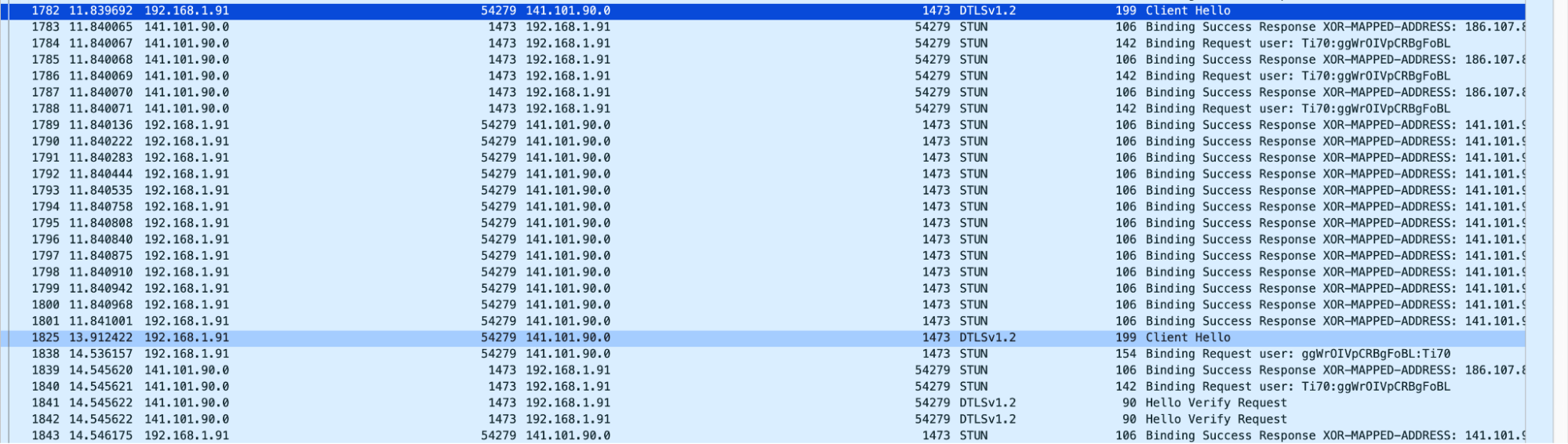
Fippo and Gustavo of WebRTCHacks complained (gracefully noted) about slow replies to ICE connectivity checks in their great article as they were digging into our WHIP implementation right around our announcement in 2022:
Looking at the Wireshark dumps we see a surprisingly large amount of time pass between the first STUN request and the first STUN response – it was 1.8 seconds in the screenshot below.
In other tests, it was shorter, but still 600ms long.
After that, the DTLS packets do not get an immediate response, requiring multiple attempts. This ultimately leads to a call setup time of almost three seconds – way above the global average of 800ms Fippo has measured previously (for the complete handshake, 200ms for the DTLS handshake). For Cloudflare with their extensive network, we expected this to be way below that average.
Gustavo and Fippo observed our solution to this problem of different parts of the WebRTC negotiation landing on different servers. Since Cloudflare Calls unbundles the WebRTC protocol to make the entire network act like a single computer, at this critical moment, we need to form consensus across the network. We form consensus by configuring every server to handle any incoming PeerConnection just in time. When a packet arrives, if the server doesn’t know about it, it quickly learns about the negotiated parameters from another server, such as the ufrag and the DTLS fingerprint from the SDP, and responds with the appropriate response.
Getting faster
Even though we’ve sped up the process of forming consensus across the Cloudflare network, any delays incurred can still have weird side effects. For example, up until a few months ago, delays of a few hundred milliseconds caused slow connections in Chrome.
A connectivity check packet delayed by a few hundred milliseconds signals to Chrome that this is a high latency network, even though every other STUN message after that was replied to in less than 5-10ms. Chrome thus delays sending a USE-CANDIDATE attribute in the responses for a few seconds, degrading the user experience.
Fortunately, Chrome also sends DTLS ClientHello before USE-CANDIDATE (behavior we’ve seen only on Chrome), so to help speed up Chrome, Calls uses DTLS packets in place of STUN packets with USE-CANDIDATE attributes.
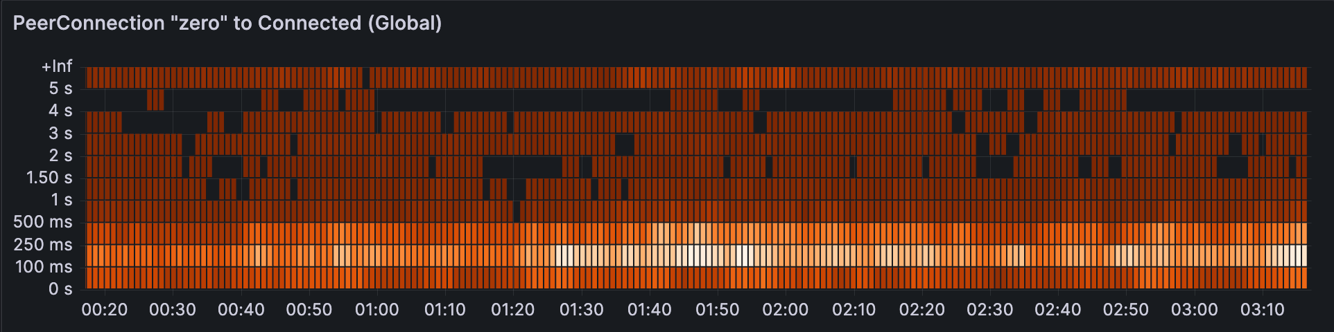
After solving this issue with Chrome, PeerConnections globally now take about 100-250ms to get connected. This includes all consensus management, STUN packets, and a complete DTLS handshake.
Sessions and Tracks are the building blocks of Cloudflare’s SFU, not rooms
Once a PeerConnection is established to Cloudflare, we call this a Session. Many media Tracks or DataChannels can be published using a single Session, which returns a unique ID for each. These then can be subscribed to over any other PeerConnection anywhere around the world using the unique ID. The tracks can be published or subscribed anytime during the lifecycle of the PeerConnection.
In the background, Cloudflare takes care of scaling through a fan-out architecture with cascading trees that are unique per track. This structure works by creating a hierarchy of nodes where the root node distributes the stream to intermediate nodes, which then fan out to end-users. This significantly reduces the bandwidth required at the source and ensures scalability by distributing the load across the network. This simple but powerful architecture allows developers to build anything from 1:1 video calls to large 1:many or many:many broadcasting scenarios with Calls.
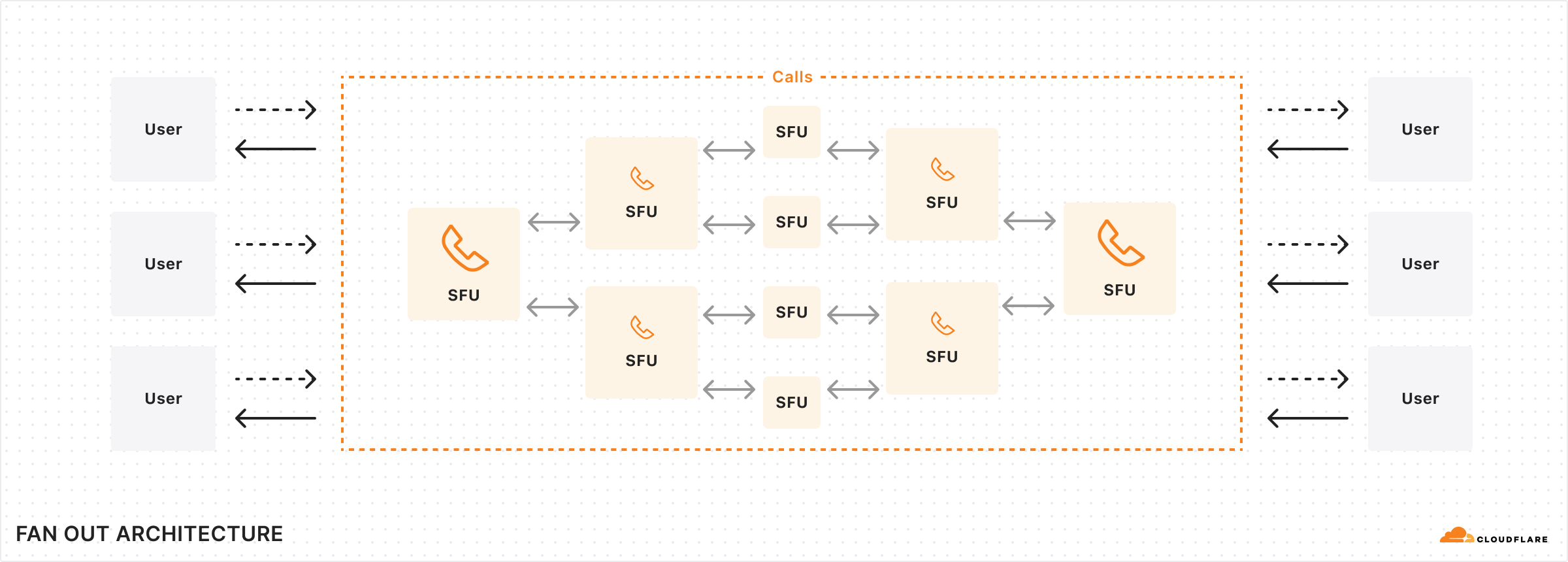
There is no “room” concept in Cloudflare Calls. Each client can add as many tracks into a PeerConnection as they’d like. The limit is the bandwidth available between Cloudflare and the client, which is practically limited by the client side every time. The signaling or the concept of a “room” is left to the application developer, who can choose to pull as many tracks as they’d like from the tracks they have pushed elsewhere into a PeerConnection. This allows developers to move participants into breakout rooms and then back into a plenary room, and then 1:1 rooms while keeping the same PeerConnection and MediaTracks active.
Cloudflare offers an unopinionated approach to bandwidth management, allowing for greater control in customizing logic to suit your business needs. There is no active bandwidth management or restriction on the number of tracks. The WebRTC Stats API provides a standardized way to access data on packet loss and possible congestion, enabling you to incorporate client-side logic based on this information. For instance, if poor Wi-Fi connectivity leads to degraded service, your front-end could inform the user through a notice and automatically reduce the number of video tracks for that client.
“NACK shield” at the edge
The Internet can’t guarantee timely and orderly delivery of packets, leading to the necessity of retransmission mechanisms, particularly in protocols like TCP. This ensures data eventually reaches its destination, despite possible delays. Real-time systems, however, need special consideration of these delays. A packet that is delayed past its deadline for rendering on the screen is worthless, but a packet that is lost can be recovered if it can be retransmitted within a very short period of time, on the order of milliseconds. This is where NACKs come to play.
A WebRTC client receiving data constantly checks for packet loss. When one or more packets don’t arrive at the expected time or a sequence number discontinuity is seen on the receiving buffer, a special NACK packet is sent back to the source in order to ask for a packet retransmission.
In a peer-to-peer topology, if it receives a NACK packet, the source of the data has to retransmit packets for every participant. When an SFU is used, the SFU could send NACKs back to source, or keep a complex buffer for each client to handle retransmissions.
This gets more complicated with Cloudflare Calls, since both the publisher and the subscriber connect to Cloudflare, likely to different servers and also probably in different locations. In addition, there is a possibility of other Cloudflare data centers in the middle, either through Argo, or just as part of scaling to many subscribers on the same track.
It is common for SFUs to backpropagate NACK packets back to the source, losing valuable time to recover packets. Calls goes beyond this and can handle NACK packets in the location closest to the user, which decreases overall latency. The latency advantage gives more chance for the packet to be recovered compared to a centralized SFU or no NACK handling at all.
Since there is possibly a number of Cloudflare data centers between clients, packet loss within the Cloudflare network is also possible. We handle this by generating NACK packets in the network. With each hop that is taken with the packets, the receiving end can generate NACK packets. These packets are then recovered or backpropagated to the publisher to be recovered.
Cloudflare Calls does TURN over Anycast too
Separately from the SFU, Calls also offers a TURN service. TURN relays act as relay points for traffic between WebRTC clients like the browser and SFUs, particularly in scenarios where direct communication is obstructed by NATs or firewalls. TURN maintains an allocation of public IP addresses and ports for each session, ensuring connectivity even in restrictive network environments.
Cloudflare Calls’ TURN service supports a few ports to help with misbehaving middleboxes and firewalls:
- TURN-over-UDP over port 3748 (standard), and also port 53
- TURN-over-TCP over ports 3748 and 80
- TURN-over-TLS over ports 5349 and 443
TURN works the same way as Calls, available over anycast and always connecting to the closest datacenter.
Pricing and how to get started
Cloudflare Calls is now in open beta and available in your Cloudflare Dashboard. Depending on your use case, you can set up an SFU application and/or a TURN service with only a few clicks.
To kick off its open beta phase, Calls is available at no cost for a limited time. Starting May 15, 2024, customers will receive the first terabyte each month for free, with any usage beyond that charged at $0.05 per real-time gigabyte. Beta customers will be provided at least 30 days to upgrade from the free beta to a paid subscription. Additionally, there are no charges for in-bound traffic to Cloudflare. For volume pricing, talk to your account manager.
Cloudflare Calls is ideal if you are building new WebRTC apps. If you have existing SFUs or TURN infrastructure, you may still consider using Calls alongside your existing infrastructure. Building a bridge to Calls from other places is not difficult as Cloudflare Calls supports standard WebRTC APIs and acts like just another WebRTC peer.
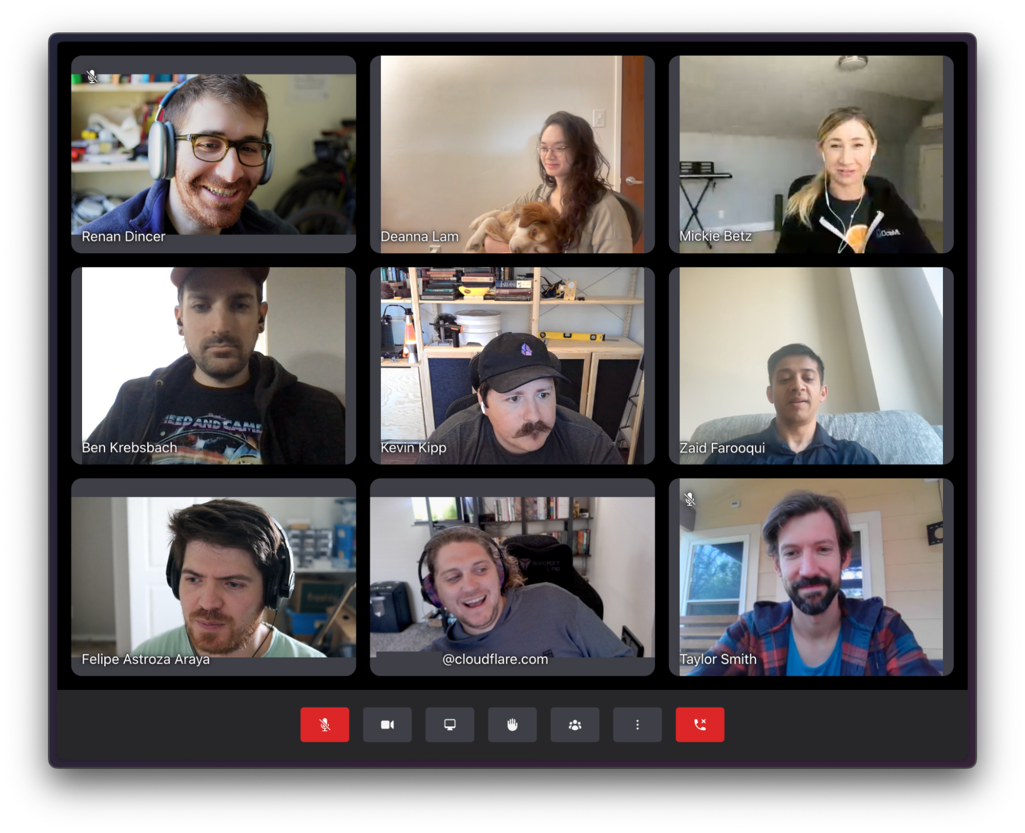
We understand that getting started with a new platform is difficult, so we’re also open sourcing our internal video conferencing app, Orange Meets. Orange Meets supports small and large conference calls by maintaining room state in Workers Durable Objects. It has screen sharing, client-side noise-canceling, and background blur. It is written with TypeScript and React and is available on GitHub.
We’re hiring
We think the current state of Cloudflare Calls enables many use cases. Calls already supports publishing and subscribing to media tracks and DataChannels. Soon, it will support features like simulcasting.
But we’re just scratching the surface and there is so much more to build on top of this foundation.
If you are passionate about WebRTC (and other real-time protocols!!), the Media Platform team building the Calls product at Cloudflare is hiring and would love to talk to you.


 Andrea Filippo is a Partner Solutions Architect at AWS supporting Public Sector partners and customers in Italy. He focuses on modern data architectures and helping customers accelerate their cloud journey with serverless technologies.
 Emanuele is a Solutions Architect at AWS, based in Italy, after living and working for more than 5 years in Spain. He enjoys helping large companies with the adoption of cloud technologies, and his area of expertise is mainly focused on Data Analytics and Data Management. Outside of work, he enjoys traveling and collecting action figures.
 Varsha Velagapudi is a Senior Technical Product Manager with Amazon DataZone at AWS. She focuses on improving data discovery and curation required for data analytics. She is passionate about simplifying customers’ AI/ML and analytics journey to help them succeed in their day-to-day tasks. Outside of work, she enjoys nature and outdoor activities, reading, and traveling.

 Andries Engelbrecht is a Principal Partner Solutions Architect at Snowflake and works with strategic partners. He is actively engaged with strategic partners like AWS supporting product and service integrations as well as the development of joint solutions with partners. Andries has over 20 years of experience in the field of data and analytics.
 Deenbandhu Prasad is a Senior Analytics Specialist at AWS, specializing in big data services. He is passionate about helping customers build modern data architectures on the AWS Cloud. He has helped customers of all sizes implement data management, data warehouse, and data lake solutions.
 Brian Dolan joined Amazon as a Military Relations Manager in 2012 after his first career as a Naval Aviator. In 2014, Brian joined Amazon Web Services, where he helped Canadian customers from startups to enterprises explore the AWS Cloud. Most recently, Brian was a member of the Non-Relational Business Development team as a Go-To-Market Specialist for Amazon DynamoDB and Amazon Keyspaces before joining the Analytics Worldwide Specialist Organization in 2022 as a Go-To-Market Specialist for AWS Glue.
 Nidhi Gupta is a Sr. Partner Solution Architect at AWS. She spends her days working with customers and partners, solving architectural challenges. She is passionate about data integration and orchestration, serverless and big data processing, and machine learning. Nidhi has extensive experience leading the architecture design and production release and deployments for data workloads.
 Scott Teal is a Product Marketing Lead at Snowflake and focuses on data lakes, storage, and governance.
 Arun Lakshmanan is a Search Specialist with Amazon OpenSearch Service based out of Chicago, IL. He has over 20 years of experience working with enterprise customers and startups. He loves to travel and spend quality time with his family.
 Madhan Kumar Baskaran works as a Search Engineer at AWS, specializing in Amazon OpenSearch Service. His primary focus involves assisting customers in constructing scalable search applications and analytics solutions. Based in Bengaluru, India, Madhan has a keen interest in data engineering and DevOps.