Today, we’re announcing the next generation of AWS Resilience Hub with a significantly expanded experience that brings together a new application model, dependency discovery assessment, generative AI-powered failure mode analysis, modular resilience policies, and organization-wide reporting.
Organizations running hundreds of applications share a common challenge: availability is a top concern, yet there is no consistent way to set resilience goals, measure progress, or prove compliance across a portfolio. Teams set different standards, use different tools, and struggle to exchange information about whether applications actually meet expectations.
The next generation of AWS Resilience Hub changes this by giving Site Reliability Engineers (SREs) and development teams a structured way to align on resilience policy expectations, help application teams achieve them, and demonstrate compliance through testing. With integration into AWS Organizations, teams can now evaluate resilience at scale, identify failure modes, discover hidden dependencies, and report on progress across the enterprise.
The next generation of Resilience Hub walks you through your resilience journey and to help you there are the following concepts built into it.
Resilience policy: You can define your resilience expectations through modular, composable requirements. Rather than choosing a single rigid policy type, you construct policies by selecting the requirements that matter to your application, such as service level objective (SLO), multi-AZ and multi-Region disaster recovery, and data recovery requirements.
Business-level understanding: You can use new application modeling through critical end-user paths that map directly to business outcomes. Systems represent a business application, user journeys describe critical business paths, and services are the deployable units comprising AWS resources, code, and observability. Resilience Hub automatically discovers and maps them into a topology showing how resources connect.
AI failure mode assessments: You can run generative AI-powered assessments that analyze your services against your defined resilience policies, AWS Well-Architected best practices, and the AWS Resilience Analysis Framework. These assessments identify potential failure modes and provide actionable recommendations.
Dependency discovery assessment: You can automatically discover AWS services, internal endpoints, and third-party endpoints that your services depend on. This dependency assessment uses DNS query log analysis to identify dependencies you may not know about—including unexpected cross-region calls or critical third-party dependencies.
The next generation of AWS Resilience Hub in action To get started, you configure a resilience policy, set up your first system and service, run a failure mode assessment, review the results, and implement the findings.
Before you begin, you should set up the invoker IAM role, which grants Resilience Hub read-only access to your AWS resources, cross-account roles (if not using AWS Organizations), or service-linked roles (SLRs) with AWS Organizations. Resilience Hub also integrates with AWS Organizations to enable organization-wide resilience management from a single delegated administrator account. This eliminates the need to log in to individual accounts to assess resilience posture across your enterprise. To learn more, visit For prerequisite details in the AWS Resilience Hub User Guide.
To configure a resilience policy, choose Create policy in the Policies menu through the AWS Resilience Hub console. Enter a policy name, description, and choose resilience requirements. For example, you can create a reusable policy for multi-Region disaster recovery used in financial applications—including 99.95% availability SLO, 15-minutes RTO, 5-minutes RPO for multi-Region disaster recovery, and disaster recovery approach that aligns with your RTO and RPO requirements.
If you choose data recovery requirements, you can define the data recovery time objective for restoring from backups for each service associated with this policy.
To create your first system representing your business application, choose Create a system in the Systems menu. Optionally, you can enable AWS Organizations account access for this system.
Now you can create a service that represents a deployable unit, like one of your microservices, and associate it with your system, and tell Resilience Hub where to find your resources. Enter a service name, for example, stock-exchange-service, choose your resilience policy and invoker AWS IAM role name. You can choose service Regions, service resources such as your resource tags, AWS CloudFormation stack, Terraform state file location, or Amazon EKS cluster and namespace.
When you enable dependency discovery for this service, AWS examines your VPC query logs for the VPCs associated with the resources in your service. You can disable this feature anytime from the dependency discovery settings in the service details page.
Now, you can run your first assessment with the service creation complete and a policy applied. Choose Run failure mode assessment in your service page and wait for the assessment to complete.
During the assessment, Resilience Hub assumes your invoker role, reads resources from your configured input sources, identifies parent-child relationships, queries the application topology service to map connections between resources, and builds a topology showing data flow, containment, and permissions.
By choosing Service topology, you can see service resources grouped by service functions in the graph, table, or JSON format.
By choosing Failure mode guidance, you can add assertions used to guide the agents while performing the failure mode assessment. Assertions are either generated by the agent or added by users. You can update them to improve assessment accuracy.
Once the assessment is complete, you can review findings and recommendations in the Assessment tab of your service page. Each finding tells you what the failure mode is, why it matters for your architecture, how to fix it, and which policy requirement it relates to.
You can choose Mark as resolved to implement the recommendation or Mark as irrelevant if the finding doesn’t apply to your use case.
If you’re an existing Resilience Hub customer, Resilience Hub provides migration APIs to simplify the transition of your previous applications. These APIs convert your previous assessment policies to new resilience policies, map your previous applications to the new model, such as multiple related applications to one system with multiple services.
Now available The next generation of AWS Resilience Hub is now generally available in AWS commercial Regions where Resilience Hub is available. For Regional availability and the future roadmap, visit the AWS Capabilities by Region.
Resilience Hub uses a new service-based pricing model. Pricing includes two failure mode assessments per month for services, and optionally automated dependency assessment. You can try AWS Resilience Hub free. For pricing details, visit the AWS Resilience Hub pricing page.
Network administrators face a persistent challenge: maintaining domain blocklists and allowlists that keep pace with the internet. New websites and services emerge daily, and keeping these lists current requires constant manual updates that leave gaps in coverage. This challenge intensifies when managing access to rapidly evolving categories like AI services, where new tools launch on a regular basis.
AWS Network Firewall is a managed, stateful network firewall and intrusion detection and prevention service for fine-grained control of your virtual private cloud (VPC) network traffic. With URL and domain category filtering, security teams can use predefined categories to control access instead of managing individual domains. AWS-managed URL and domain categories stay current automatically as new domains are registered, removing the need for manual list maintenance.
This feature is especially useful for organizations navigating AI governance. Instead of manually tracking every new AI service, you can control access to the entire Artificial Intelligence and Machine Learning category while creating exceptions for approved services. The same approach works for social media, streaming sites, gambling, and dozens of other categories, all with built-in audit trails for compliance reporting.
In this post, we walk through URL and domain category filtering configurations for AWS Network Firewall, from basic rules to exception handling and monitoring strategies that give you visibility into how your workloads interact with external services.
Streamlined policy management with predefined categories
With URL and domain category filtering, you control website access using predefined categories instead of individually specifying sites in a domain list rule group. You can select from AWS-managed categories such as Social Networking, Gambling, or Artificial Intelligence and Machine Learning to implement and maintain filtering policies. AWS keeps these categories current automatically, so you don’t need to update firewall policies when new domains are registered.
Network Firewall offers two category filtering options. Domain category filters by domain name using the TLS Server Name Indication (SNI) field, with no decryption required. URL category filters by the full URL path, which requires TLS inspection for HTTPS traffic. To keep things straightforward, this post focuses on domain category filtering. To set up URL category filtering with TLS inspection, see Creating a TLS inspection configuration in Network Firewall.
Prerequisites
To follow the steps in this post, start by making sure that you have the following prerequisites in place:
An existing Network Firewall deployment: This walkthrough assumes you have an existing Network Firewall deployment to filter egress traffic flows from your Amazon Virtual Private Cloud (Amazon VPC) in place. If you aren’t already using Network Firewall, see Getting started with AWS Network Firewall to set up your firewall before proceeding.
The HOME_NET variable set correctly at the firewall policy level: The rules in this post use the $HOME_NET variable to scope traffic to your internal network. In the AWS Management Console for Amazon VPC, select your firewall policy under the Firewall policies tab, select the Details tab, and check the policy variables section under HOME_NET variable override values. We recommend setting this to all RFC 1918 private IP address ranges: 10.0.0.0/8, 172.16.0.0/12, and 192.168.0.0/16. When you set $HOME_NET at the policy level, all rule groups associated with that policy inherit the value automatically. Network Firewall automatically maps $EXTERNAL_NET to the inverse of $HOME_NET, so configuring HOME_NET correctly also configures $EXTERNAL_NET.
Figure 1: Firewall policy details tab showing the HOME_NET variable override values set to RFC 1918 private IP address ranges
Create a category rule using the console rule builder
To get started quickly, you can create a domain category rule using the console’s built-in rule builder. In this example, we create a single alert rule for the Artificial Intelligence and Machine Learning category.
In the left navigation, scroll to Network Firewall and select Rule groups.
Choose Create rule group.
For Rule group type, select Stateful rule group.
For Rule group format, select Standard stateful rules.
For Rule evaluation order, select Strict order. Choose Next.
Figure 2: Create Network Firewall rule group page showing Stateful rule group type, Standard stateful rules format, and Strict order evaluation selected
Enter Domain-Category-Rules for the Name, Domain Category Rules for the Description, and 50 for the Capacity. Choose Next.
In the rule group editor, select the Category Matching radio button.
Under Category Matching, select Match all selected categories.
Under AWS category type, select Domain Category from the dropdown.
Under Categories, select Artificial Intelligence and Machine Learning.
For Protocol, select TLS.
For Source, select Custom, then enter $HOME_NET in the dialog box.
Set the Destination IP to Any.
For Action, select Alert.
Choose Add rule to add this rule to the rule group. Choose Next.
Figure 3: Completed category matching rule showing TLS protocol, $HOME_NET source, Any destination, and Alert action added to the rule group
Under Customer managed key, leave the default setting (Customize encryption settings should remain unchecked).
Under Add tags – optional, leave the default setting of no tags.
Choose Next, then Create rule group.
This rule generates an alert log entry each time a connection matches a domain in the Artificial Intelligence and Machine Learning category. It doesn’t block traffic. To block traffic, change the action to Drop or Reject in step 15.
Creating the same rule using Suricata compatible rule strings
The following walkthrough creates the same alert rule you built with the console rule builder, this time using a Suricata rule string.
In the Amazon VPC console, navigate to Network Firewall, then select Network Firewall rule groups.
Choose Create rule group.
For Rule group type, select Stateful rule group.
For Rule group format, select Suricata compatible rule string.
For Rule evaluation order, select Strict order. Choose Next.
Figure 4: Create Network Firewall rule group page showing Stateful rule group type, Suricata compatible rule string format, and Strict order evaluation selected
Enter Suricata-Domain-Category-Rules for the Name, Suricata Domain Category Rules for the Description, and 50 for the Capacity. Choose Next.
Leave the Rule variables section empty. The $HOME_NET variable is inherited from the firewall policy, as configured in the prerequisites.
Leave IP set references empty.
Paste the following rule into the Suricata compatible rule string editor:
alert tls $HOME_NET any -> $EXTERNAL_NET any (msg:"Artificial Intelligence and Machine Learning Category"; aws_domain_category:Artificial Intelligence and Machine Learning; sid:1000001;)
Choose Next.
Figure 5: Suricata compatible rule string editor with the domain category alert rule pasted in and the rule variables section left empty
Under Customer managed key, leave the default setting (Customize encryption settings should remain unchecked).
Under Add tags – optional, leave the default setting of no tags. Choose Next.
Choose Create rule group.
After creating the rule group, return to your firewall policy and add it under Stateful rule groups. We recommend associating new rule groups in a development or test environment first to validate behavior before deploying to production.
The following table explains each component of this rule:
alert
Action: generate an alert log entry when the rule matches. Other actions include pass, drop, and reject.
tls
Protocol: inspect TLS traffic, matching against the SNI field in the TLS Client Hello.
$HOME_NET any -> $EXTERNAL_NET any
Source and destination: match traffic from any internal IP address (HOME_NET) and port to any external IP address (EXTERNAL_NET) and port. The HOME_NET variable defines your internal network ranges, and the EXTERNAL_NET variable is automatically set to the inverse.
msg:”Artificial Intelligence and Machine Learning Category”
The message written to the alert log when this rule is triggered.
aws_domain_category:Artificial Intelligence and Machine Learning
The AWS-managed domain category to match against. The firewall looks up the destination domain in the category database and matches if the domain belongs to this category.
sid:1000001
A unique signature ID for this rule. Each rule in a rule group must have a unique SID.
Managing exceptions for approved services
You can manage exceptions to keep business-critical websites accessible. For example, say you need to allow access to OpenAI while blocking all other AI and ML traffic. To do this, return to the Suricata-Domain-Category-Rules rule group you created earlier and replace the basic alert rule with the following ruleset. Select the Suricata-Domain-Category-Rules rule group, under the Rules section, choose Edit.
Figure 6: Selecting Suricata-Domain-Category-Rules rule group to edit with new rules
Paste in the following rules and choose Save rule group.
# Allow OpenAI (TLS)
pass tls $HOME_NET any -> $EXTERNAL_NET any (tls.sni; dotprefix; content:".openai.com"; nocase; endswith; flow:to_server; alert; msg:"Allow OpenAI over TLS"; sid:1000001;)

# Allow OpenAI (HTTP)
pass http $HOME_NET any -> $EXTERNAL_NET any (http.host; dotprefix; content:".openai.com"; nocase; endswith; flow:to_server; alert; msg:"Allow OpenAI over HTTP"; sid:1000002;)

# Block all other AI/ML category traffic (TLS)
reject tls $HOME_NET any -> $EXTERNAL_NET any (msg:"Block non-approved AI/ML sites over TLS"; aws_domain_category:Artificial Intelligence and Machine Learning; flow:to_server; alert; sid:1000003;)

# Block all other AI/ML category traffic (HTTP)
reject http $HOME_NET any -> $EXTERNAL_NET any (msg:"Block non-approved AI/ML sites over HTTP"; aws_url_category:Artificial Intelligence and Machine Learning; flow:to_server; alert; sid:1000004;)
Figure 7: Suricata compatible rule string editor with the exception-based ruleset containing pass rules for OpenAI and reject rules for the AI/ML category
With strict order evaluation, the firewall evaluates rules in the order you define them. The pass rules for OpenAI appear first, so matching traffic is allowed before the broader category block rules run.
To verify the rules are working as expected, test from a host that routes traffic through your network firewall. These commands suppress the response body and check the exit code of the curl request. If curl completes a TCP connection, it prints CONNECTION ALLOWED. If the firewall resets the connection, curl exits with a non-zero code and prints CONNECTION BLOCKED.
A request to openai.com should succeed because it matches the pass rule:
When you add a domain category rule to your firewall policy, Network Firewall performs a category lookup for every connection that matches the rule’s protocol and IP specifications. The rules in this post match on $HOME_NET any -> $EXTERNAL_NET any, which means the firewall looks up the category for all outbound traffic originating from your internal network. This is why it’s important to have the $HOME_NET variable configured correctly at the firewall policy level. With this configuration, a single category rule is enough for category metadata to appear in your firewall logs across all matching connections, not just connections that match the specific category in your rule.
Each log entry includes an aws_category field containing a JSON array of all categories the destination domain belongs to. A single domain can map to multiple categories. For example, a request to chat.mistral.ai produces a log entry with “aws_category": "[\"Social Networking\",\"Artificial Intelligence and Machine Learning\"]” because that domain belongs to both categories.
The following sample log entry shows what a blocked request to chat.mistral.ai looks like using the exception-based rules from the previous section. The alert.signature field contains the rule’s msg value, and the aws_category field lists all categories the destination domain belongs to:
The aws_category field shows the domain belongs to both the “Social Networking” and “Artificial Intelligence and Machine Learning” categories. The verdict field confirms the connection was dropped with a TCP reset sent to the client.
Traffic that matches a pass rule with the alert keyword also generates a log entry with the aws_category field populated. For example, a connection to chat.openai.com that matches the OpenAI exception rule from the earlier section produces a log entry with alert.action set to “allowed” and the same category metadata. This means your queries capture both blocked and allowed traffic.
Querying logs with CloudWatch Logs Insights
If you send your firewall logs to Amazon CloudWatch Logs, you can use CloudWatch Logs Insights to analyze category traffic patterns. A single connection can generate multiple log entries (for example, a reject rule log and a default action log for the same flow), so the following queries deduplicate by flow_id to count each connection only once. Because a single domain can belong to multiple categories, results are grouped by category combination. For example, traffic to a domain categorized as both “Social Networking” and “Artificial Intelligence and Machine Learning” appears as a single combined entry.
To get started, navigate to the CloudWatch console. In the left navigation pane under Logs, select Logs Insights. Under Query scope, leave Log group name selected, then select your AWS Network Firewall alert logs log group. For the time window, we recommend starting with the default of 1 hour to keep the queries light. Enter each of the following queries into the editor and choose Run query to review the results. Note that CloudWatch Logs Insights queries incur charges based on the amount of data scanned. See Amazon CloudWatch pricing for details.
Most accessed categories
This query shows which category combinations your workloads connect to most frequently:
fields @timestamp, event.aws_category, event.flow_id
| filter ispresent(event.aws_category) and event.aws_category != "[]"
| stats latest(event.aws_category) as categories by event.flow_id
| stats count(*) as connections by categories
| sort connections desc
| limit 20
Figure 8: CloudWatch Logs Insights query results showing the most frequently accessed category combinations sorted by connection count
Least accessed categories
This query reverses the sort order to surface category combinations with the fewest connections, helping you identify categories that might not be relevant to your environment or that warrant further investigation:
fields @timestamp, event.aws_category, event.flow_id
| filter ispresent(event.aws_category) and event.aws_category != "[]"
| stats latest(event.aws_category) as categories by event.flow_id
| stats count(*) as connections by categories
| sort connections asc
| limit 20
Figure 9: CloudWatch Logs Insights query results showing the least frequently accessed category combinations sorted by connection count ascending
Most accessed categories, allowed traffic only
The event.verdict.action field indicates the actual outcome of each connection:drop for blocked traffic and alert for allowed traffic. This query shows which category combinations have the most allowed connections:
fields @timestamp, event.aws_category, event.flow_id, event.verdict.action
| filter ispresent(event.aws_category) and event.aws_category != "[]"
| stats latest(event.aws_category) as categories, latest(event.verdict.action) as verdict by event.flow_id
| filter verdict = "alert"
| stats count(*) as connections by categories
| sort connections desc
| limit 20
Figure 10: CloudWatch Logs Insights query results showing the most accessed category combinations filtered to allowed traffic only
Most accessed categories, blocked traffic only
The same query filtered to blocked connections. Change the verdict filter to drop:
fields @timestamp, event.aws_category, event.flow_id, event.verdict.action
| filter ispresent(event.aws_category) and event.aws_category != "[]"
| stats latest(event.aws_category) as categories, latest(event.verdict.action) as verdict by event.flow_id
| filter verdict = "drop"
| stats count(*) as connections by categories
| sort connections desc
| limit 20
Figure 11: CloudWatch Logs Insights query results showing the most accessed category combinations filtered to blocked traffic only
Drill down into a specific category
This query uses a like filter to find all traffic where the aws_category field contains a specific category, regardless of what other categories the domain also belongs to. In this example, the query returns all domains your workloads have connected to that map to the Artificial Intelligence and Machine Learning category, broken down by domain and verdict. Replace the category name in the like filter to investigate any category.
fields @timestamp, event.tls.sni, event.aws_category, event.verdict.action, event.flow_id
| filter ispresent(event.aws_category) and event.aws_category like /Artificial Intelligence and Machine Learning/
| stats latest(event.tls.sni) as sni, latest(event.verdict.action) as verdict by event.flow_id
| stats count(*) as connections by sni, verdict
| sort connections desc
| limit 20
Figure 12: CloudWatch Logs Insights query results showing a drill down into the Artificial Intelligence and Machine Learning category with connections broken down by domain and verdict
Bandwidth consumption by category
This query shows which category combinations consume the most egress bandwidth. It correlates flow logs (which contain byte counts) with alert logs (which contain category data) using the shared flow_id field. To run this query, select both your alert log group and your flow log group in CloudWatch Logs Insights.
fields @timestamp
| filter ispresent(event.netflow.bytes) or ispresent(event.aws_category)
| stats sum(event.netflow.bytes) as flowBytes, latest(event.aws_category) as categories by event.flow_id
| filter ispresent(categories) and categories != "[]"
| stats sum(flowBytes) as totalBytes by categories
| sort totalBytes desc
| limit 20
Figure 13: CloudWatch Logs Insights query results showing bandwidth consumption by category combination sorted by total bytes descending
These queries help you identify which categories your workloads access by volume, surface blocked and allowed traffic patterns, and pinpoint where the bulk of your egress bandwidth is going.
Conclusion
In this post, you walked through how to set up URL and domain category filtering on AWS Network Firewall, from creating your first category rule using both the console rule builder and Suricata compatible rule strings, to managing exceptions for approved services and monitoring category traffic patterns with CloudWatch Logs Insights. With AWS-managed categories that stay current automatically, you can control access to broad classes of websites without maintaining individual domain lists, and the built-in aws_category log field gives you the visibility to track how your workloads interact with external services.
This feature is available in all AWS commercial regions where AWS Network Firewall is supported.
Today, we’re announcing the next generation of Amazon OpenSearch Serverless, a fully managed search and vector engine designed for customers building AI agents. The next generation of OpenSearch Serverless scales from zero to thousands of requests per second and back to zero when idle, offering up to 60% cost savings compared to the cost of OpenSearch Service clusters provisioned for peak capacity.
The next generation of OpenSearch Serverless creates resources in seconds and scales capacity up to 20 times faster than the previous generation. With instant resource creation and native integrations with AI development platforms like Vercel and Kiro, you can deploy production-ready search and vector backends for your AI agents in minutes without managing infrastructure.
The next generation of OpenSearch Serverless in action To get started with the next generation of OpenSearch Serverless, choose Create collection in the Serverless menu in the Amazon OpenSearch Service console.
Create NextGen collection with instant auto scaling and scale-to-zero for cost optimization. At launch, we support full-text search and vector search only for the collection type. If you want to use the existing OpenSearch Serverless infrastructure, choose Switch to Classic.
Choose Express create, the fastest way to create collection. No configuration is required—the default settings and matching security policies are applied automatically. Some configuration options can be changed later.
When you choose Create collection, OpenSearch Serverless will provision resources in seconds.
You can also create a collection of OpenSearch Serverless with AWS Command Line Interface (AWS CLI) or AWS SDKs. Here is a sample CLI command to create a collection group.
Building your agents faster with OpenSearch Serverless To support building production-ready agent applications in Vercel, you can now create a new OpenSearch collection or connect your existing OpenSearch Serverless collection within the Vercel console. Create a search backend in seconds and add features on-demand as your application grows. To learn more, visit AWS for Vercel.
You can go from idea to working prototype in minutes using Claude Code, Cursor, and Kiro. OpenSearch Agent Skills provide a repository of skills that bring OpenSearch intelligence directly into your agent. Each skill encapsulates domain knowledge, best practices, and multi-step execution logic for a specific workflow–so your agent not only gets results, but understands how they were achieved. You can also use the OpenSearch Launchpad in Kiro Powers to accelerate search applications with guided, end-to-end architecture planning.
Now available The next generation of Amazon OpenSearch Serverless is generally available today and is available in all AWS commercial Regions where Amazon OpenSearch Serverless is currently available.
The next generation of OpenSearch Serverless charges for the compute you use in OpenSearch Compute Units (OCUs) for indexing, search, and GPU acceleration. You are charged separately for storage in GB-month. For more information, see Amazon OpenSearch Service Pricing.
Audience note: This is the deep-dive technical launch post. For a shorter overview of what changed and why, see the related post on the AWS News Blog.
Today, we are announcing a ground-up re-architecture of Amazon OpenSearch Serverless that delivers up to 20 times faster autoscaling, scale to zero, and up to 60% lower cost than provisioning clusters for peak load. Amazon OpenSearch Service is a fully managed, open source retrieval engine that unifies vector, lexical, hybrid, and agentic search, delivering low-latency, accurate and relevant results. Amazon OpenSearch Serverless is an automatically scaled deployment option.
Modern workloads are increasingly dynamic and unpredictable. An ecommerce platform sees a 10x traffic spike during a flash sale. An artificial intelligence (AI) agent triggers hundreds of concurrent vector queries while reasoning through a multi-step task, then goes idle. A multi-tenant SaaS application serves dozens of tenants with wildly different activity patterns. These workloads need infrastructure that scales up to meet demand and releases resources when demand drops.
That is why we rebuilt the Amazon OpenSearch Serverless architecture from the ground up. The new architecture decouples compute from storage. The service provisions infrastructure in seconds instead of minutes, and scales compute all the way to zero when your application is idle. In this post, we walk through the new architecture, what it means for your applications, and how to get started with a hands-on tutorial.
With this launch, Amazon OpenSearch Serverless introduces two named architectures. Existing collections are now referred to as Classic collections. The new architecture is called NextGen and is now the default when you create a new collection via the AWS Console. You can use NextGen architecture in the API by specifying --generation NEXTGEN in the CLI. To continue using the Classic architecture, specify --generation CLASSIC in the CLI or omit the optional --generation parameter.
What this means for your applications
The new architecture delivers improvements across three pillars: performance, cost, and a simplified user experience.
Performance: Autoscaling in seconds
An OpenSearch Compute Unit (OCU) is the unit of compute capacity that powers your indexing and search workloads. Amazon OpenSearch Serverless now provisions additional OCUs in seconds. When traffic arrives, the service adds resources in line with demand instead of reacting after a worker is already under pressure. The same mechanism scales the infrastructure back down quickly when traffic drops. The new architecture scales capacity up to 20 times faster than the previous architecture, so your users experience consistent performance during traffic surges, and you stop paying for capacity when you no longer need it.
Cost efficiency: Pay only for what you use
Indexing, search, storage, and Vector Index GPU-Acceleration are metered and billed independently, so you can see and optimize each dimension of your workload separately.
Decoupled compute and storage: OpenSearch Serverless now has full decoupling between compute and storage, allowing OCUs to scale up and down irrespective of the amount of data stored in a collection. This is powered by a new storage layer that is accessible to both indexing and search OCUs. You can now have multiple indices with data indexed in them but not pay any compute costs if you are not actively indexing or searching data. For workloads with significant idle time, the new architecture can reduce infrastructure costs by up to 60% compared to the cost of provisioning OpenSearch Service domains for peak capacity.
Scale to zero: When no requests arrive within the idle timeout window (10 minutes), the service releases compute resources and your OCU usage scales to 0. When traffic resumes, capacity is back in approximately 10 seconds. During this window, the service queues incoming requests and serves them once capacity is available; it does not drop them. If you anticipate a burst of traffic, for example before a scheduled batch job or a marketing campaign, you can send a lightweight query (such as a match_all with size=1) to warm the collection before your application starts sending production traffic. This reduces the latency your users experience on the first real request. Indexing and search scale independently. If you have no search requests, search OCUs scale to zero, even while OpenSearch Serverless maintains indexing OCUs for indexing requests, and vice versa.
GPU acceleration for vector workloads: For vector collections created in the new architecture, OpenSearch Serverless automatically uses GPU-backed compute to accelerate Hierarchical Navigable Small World (HNSW) vector index construction, significantly reducing indexing time compared to CPU-only builds. GPU acceleration kicks in automatically whenever there is an opportunity to leverage GPUs to reduce overall indexing time and cost. In the Classic architecture, you had to opt in or out of GPU acceleration at the collection level through the API. If you want to disable GPU acceleration for NextGen collections for a specific index, you can turn off the remote index build setting at the index level. GPU usage appears as a separate line item on your bill, so you have full visibility into when acceleration was active and what it cost. For more details on how GPU acceleration works and performance benchmarks, refer to Build billion-scale vector databases in under an hour with GPU acceleration on Amazon OpenSearch Service.
Simplified experience: Fewer steps to production
We also simplified the day-to-day experience of running OpenSearch Serverless:
With the new architecture, you can provision a collection and start sending requests in seconds. There is no need for capacity planning, no sizing decisions, and no waiting for infrastructure to warm up. This makes Amazon OpenSearch Serverless a natural fit for agentic workloads, where an AI agent can spin up a vector search or retrieval step on demand and expect a response without delay.
To make getting started even faster, we have introduced Express Create on the console. You supply a collection name and a collection type, choose Express Create, and your collection is active in seconds with no upfront network, encryption, or access policies to configure. You can add those later if your workload requires them.
Collection groups and collections can also be created programmatically using the AWS Command Line Interface (AWS CLI) and AWS SDKs. AWS CloudFormation support is coming soon.
The new architecture introduces two endpoint formats on the on.aws domain. The per-collection endpoint (<collectionId>.aoss.<region>.on.aws) works the same way as before with one endpoint per collection. The per-account Regional endpoint (<accountId>.aoss.<region>.on.aws) is new: it serves all of your collections through a single hostname, with the target collection identified in each request using the x-amz-aoss-collection-name or x-amz-aoss-collection-id header. This means one connection pool, one Transport Layer Security (TLS) session, and one endpoint to manage regardless of how many collections you have — a significant improvement for multi-tenant workloads where each tenant maps to its own collection. Both endpoints use standard AWS PrivateLink, so you create virtual private cloud (VPC) endpoints from the VPC console or the EC2 API just like any other AWS service. Private Domain Name System (DNS) is configured automatically, eliminating the Amazon Route 53 Private Hosted Zones, forwarding rules, and custom DNS infrastructure that were required with the original architecture. Cross-VPC, cross-account, and on-premises access all work using standard vpce-* DNS names with no additional setup.
Collection groups are the new unit of organization for your collections. You can share compute capacity across multiple collections with Collection Groups, which reduces cost for smaller collections that have complementary traffic patterns. You can also assign different AWS Key Management Service (AWS KMS) keys to collections within the same group, so you get both cost efficiency and per-collection encryption isolation. Collection groups are required when creating collections with the new architecture.
You also get the benefits of OpenSearch open-source releases without needing to manage versions and upgrades. The service tracks upstream releases automatically.
Amazon OpenSearch Serverless is also available on the Vercel Marketplace, making it straightforward for developers to add search infrastructure directly from their Vercel projects. You can link an existing AWS account through delegated access, or get started through a Limited Scope Account with USD $100 in AWS credit if you are new to AWS.
The integration creates a collection with sensible defaults, scale-to-zero billing, public endpoints, and AWS-managed encryption, and automatically sets connection details as environment variables in your Vercel project. You can choose from Search or Vector Search collection types depending on your use case, whether that is full-text search or semantic and AI-powered search.
How the architecture works
The new Amazon OpenSearch Serverless architecture separates compute from storage entirely. OCUs are stateless and read from and write to a distributed shared storage layer that is accessible to both indexing and search OCUs. The storage layer is designed for high durability, keeping your data available independently of the compute nodes that process it.
This design has two practical consequences:
Fast provisioning. New OCUs start serving requests in seconds because there is no local disk to bootstrap. The OCU mounts the shared storage layer and begins processing immediately.
Efficient scale down. Idle capacity can be released with no impact to your stored data, because the data never lived on the OCU. When traffic subsides, compute resources are released and your cost drops accordingly.
Architecture comparison
The following table summarizes the key differences between the original and new architectures:
Capability
Classic Architecture
NextGen Architecture
Minimum capacity
2 OCUs (always on)
0 OCUs (scale to zero)
Scaling speed
Minutes
Seconds
Storage
Local storage per compute node
Distributed shared storage (decoupled)
Collection organization
Individual collections (Default)
Collection groups (Optional)
Collection groups (required)
Cold start from zero
N/A (always on)
~10 seconds
Endpoint
Per-collection endpoint
Regional endpoint (static per account)
Cost vs. OpenSearch Service domain
Baseline
Up to 60% lower cost
Scaling speed (vs. Classic)
Baseline
Up to 20 times faster than baseline
Walkthrough: Create a vector collection and observe scale to zero
In this walkthrough, you create a vector search collection with Express Create, index a few sample documents with embeddings, run a k-nearest neighbor (k-NN) query, and watch the collection scale to zero in Amazon CloudWatch. The entire process takes about 10 minutes.
Prerequisites
An AWS account with permissions to create Amazon OpenSearch Serverless collections.
AWS Command Line Interface (AWS CLI) configured with appropriate credentials.
curl 7.75 or later (for built-in --aws-sigv4 support).
Step 1: Configure security policies
Create encryption, network, and data access policies. These must exist before the collection can be created.
# Create an encryption policy
aws opensearchserverless create-security-policy \
    --name product-vectors-encryption \
    --type encryption \
    --policy '{"Rules":[{"ResourceType":"collection","Resource":["collection/product-vectors"]}],"AWSOwnedKey":true}' \
    --endpoint-url "https://aoss.us-east-2.amazonaws.com" \
    --region "us-east-2"

# Create a network policy (public access for this tutorial)
aws opensearchserverless create-security-policy \
    --name product-vectors-network \
    --type network \
    --policy '[{"Rules":[{"ResourceType":"collection","Resource":["collection/product-vectors"]},{"ResourceType":"dashboard","Resource":["collection/product-vectors"]}],"AllowFromPublic":true}]' \
    --endpoint-url "https://aoss.us-east-2.amazonaws.com" \
    --region "us-east-2"

# Get your principal ARN
PRINCIPAL_ARN=$(aws sts get-caller-identity --query 'Arn' --output text)

# Create a data access policy
aws opensearchserverless create-access-policy \
    --name product-vectors-data \
    --type data \
    --policy "[{\"Rules\":[{\"ResourceType\":\"index\",\"Resource\":[\"index/product-vectors/*\"],\"Permission\":[\"aoss:CreateIndex\",\"aoss:DescribeIndex\",\"aoss:UpdateIndex\",\"aoss:DeleteIndex\",\"aoss:ReadDocument\",\"aoss:WriteDocument\"]}],\"Principal\":[\"\${PRINCIPAL_ARN}\"]}]" \
    --endpoint-url "https://aoss.us-east-2.amazonaws.com" \
    --region "us-east-2"
Note: If you use the AWS console’s Express Create workflow, these policies are created automatically.
Important: After creating the data access policy, wait approximately 30 to 60 seconds for the policy to propagate before making API calls to the collection. If you receive a 403 Forbidden error, wait and retry.
Step 2: Create a collection group and collection
Create a collection group with scale-to-zero capacity limits, then create a vector search collection within it.
# Create a collection group with scale-to-zero enabled (min OCU = 0)
aws opensearchserverless create-collection-group \
    --name product-search-cg \
    --generation NEXTGEN \
    --standby-replicas ENABLED \
    --capacity-limits "minIndexingCapacityInOCU=0,maxIndexingCapacityInOCU=4,minSearchCapacityInOCU=0,maxSearchCapacityInOCU=4" \
    --endpoint-url "https://aoss.us-east-2.amazonaws.com" \
    --region "us-east-2"

# Create a vector search collection in the group
aws opensearchserverless create-collection \
    --name product-vectors \
    --type VECTORSEARCH \
    --collection-group-name product-search-cg \
    --endpoint-url "https://aoss.us-east-2.amazonaws.com" \
    --region "us-east-2"
The collection status transitions to ACTIVE within seconds.
Step 3: Create a vector index
Retrieve the collection endpoint and create a k-NN index using 3-dimensional vectors:
Note: If the collection has scaled to zero, the first request might take a few seconds while capacity scales up. If the request times out, wait 10 to 15 seconds and retry.
The response returns the two most similar items, in this case, the headphone documents whose embeddings are closest to your query vector.
You can also run this query in OpenSearch UI by navigating to your collection in the Amazon OpenSearch Service console and choosing the OpenSearch UI Application URL. Then follow the steps outlined in this blog to create a workspace. Then navigate to Dev Tools and paste and run the following query.
In the response, currentCapacity.search.capacityInOcu and currentCapacity.indexing.capacityInOcu will show 0 after the collection has scaled down.
You can also navigate to the Collection groups page in the Amazon OpenSearch Service console. Choose your collection group, then scroll down to the Monitoring section. Here you can see two charts: Indexing capacity (OCUs) and Search capacity (OCUs). After 10 minutes of idle time (no indexing or search requests), both metrics drop to zero, confirming that the service has released all compute resources for your collection.
Clean up
To avoid ongoing charges, delete the resources you created in this walkthrough when you are done. Delete the collection first so the collection group becomes empty, then delete the group, then remove the security and access policies.
# Look up the collection ID, then delete the collection
COLLECTION_ID=$(aws opensearchserverless batch-get-collection \
    --names product-vectors \
    --query 'collectionDetails[0].id' \
    --output text \
    --endpoint-url "https://aoss.us-east-2.amazonaws.com" \
    --region "us-east-2")

aws opensearchserverless delete-collection \
    --id "${COLLECTION_ID}" \
    --endpoint-url "https://aoss.us-east-2.amazonaws.com" \
    --region "us-east-2"

# Look up the collection group ID, then delete the collection group
GROUP_ID=$(aws opensearchserverless batch-get-collection-group \
    --names product-search-cg \
    --query 'collectionGroupDetails[0].id' \
    --output text \
    --endpoint-url "https://aoss.us-east-2.amazonaws.com" \
    --region "us-east-2")

aws opensearchserverless delete-collection-group \
    --id "${GROUP_ID}" \
    --endpoint-url "https://aoss.us-east-2.amazonaws.com" \
    --region "us-east-2"

# Delete the security and access policies
aws opensearchserverless delete-security-policy \
    --name product-vectors-encryption \
    --type encryption \
    --endpoint-url "https://aoss.us-east-2.amazonaws.com" \
    --region "us-east-2"

aws opensearchserverless delete-security-policy \
    --name product-vectors-network \
    --type network \
    --endpoint-url "https://aoss.us-east-2.amazonaws.com" \
    --region "us-east-2"

aws opensearchserverless delete-access-policy \
    --name product-vectors-data \
    --type data \
    --endpoint-url "https://aoss.us-east-2.amazonaws.com" \
    --region "us-east-2"
Upgrading existing collections
To move to the new architecture, create a new collection group and collection, then reindex your data into it. For a step-by-step walkthrough of the reindexing process, refer to Perform reindexing in Amazon OpenSearch Serverless using Amazon OpenSearch Ingestion. Your queries and index mappings remain the same. Only the collection endpoint changes. With the new static Regional endpoint, that is a one-time update.
The new architecture supports SEARCH and VECTORSEARCH collection types. TIMESERIES is not supported at launch.
Conclusion
The new Amazon OpenSearch Serverless architecture is available today. You can create your first OpenSearch Serverless collection in seconds with Express Create, scale it to handle production traffic, and your OpenSearch Serverless compute costs drop to zero when it sits idle.
Gentoo developer Michał Górny has written a lengthy
article explaining the philosophy and purpose of the Gentoo Linux
distribution, in response to a
thread on Mastodon:
Gentoo is a source-first distribution, which means the primary
method of installing software is to build it from source. Of course,
that doesn’t mean manually building stuff, following some kind of
how-to: finding all the dependencies, installing them manually, going
through a series of magical incantations, and eventually ending up no
better than if we were installing a binary package. The package
manager takes care of all the necessary steps and more, making package
installs easy; well, at least unless something fails. But I’m
digressing…
[…] We try to build a friendly and welcoming community around Gentoo,
and we truly want using Gentoo be an enjoyable experience. We want it
to be a system that doesn’t betray you.
In a filesystem-track session at the 2026 Linux Storage,
Filesystem, Memory Management, and BPF Summit, Amir Goldstein wanted to
discuss his proposed
documentation on adding new filesystems to the kernel. There are a
number of unmaintained and untestable filesystems already in the kernel,
which are a burden to VFS-layer developers who are trying to make sweeping
changes, such as switching to folios and the “new” mount API. Goldstein’s
document is an attempt to head off the addition of filesystems that may
increase that burden down the road.
IBM has sent out a
press release touting a claimed $5 billion investment into an
operation called Project Lightwell:
Project Lightwell will establish a trusted enterprise clearinghouse
combined with a global force of engineers to identify and fix
vulnerabilities at scale. The clearinghouse will serve as a
security coordination layer, using advanced AI capabilities to
validate and test fixes across an unprecedented volume of open
source code. These capabilities will be offered through commercial
subscriptions, allowing enterprises to integrate secure patches
directly into their existing software supply chains with
enterprise-grade validation and lifecycle management.
Toward the bottom, it does also mention sharing vulnerability information
with upstream projects.
Нека го кажем така вдъхновение нямам Трудно мисля за по-натам Спомням си само откъслечни фрази Много грозота насилие и самота около мен но аз съм вече равна Тъмна агония в градината на Бог а той живее без сандали в съседния апартамент Майката е мъртва от 14 години Тази майка всъщност съм аз Стигнах дотук за да споделя за онази най-обикновена сцена от крематориума на ЦСГ Двама работници весело бутат мъртъвците към пещта чрез силни тласъци телата облечени в официални дрехи се спускат към горящите усти полегналите крака бързат напред а работниците ги догонват Една от носилките заплашително се заклаща настрани всичко беше толкова нелепо и непринудено Ние с баща ми просто преминаваме оттам
Белослава Димитрова
Белослава Димитрова (р. 1986) е поетеса и журналистка. Има три издадени книги с поезия: „Начало и край“ (2012); „Дивата природа“ (2014); „Месо и птици“ (2019). За „Дивата природа“ е номинирана за Националната награда за поезия „Иван Николов“ (2014) и е удостоена с едно от двете поощрителни отличия. За „Месо и птици“ получава Наградата за поезия „Николай Кънчев“ (2019), както и награда „Перото“ (2020) в категория „Поезия“. Белослава е един от водещите на предаването „Артефир“ в БНР. Нейни стихове са преведени на английски, немски, френски, испански, италиански, хърватски, македонски и хинди. Стихотворението „Кървав меридиан“ ще бъде част от четвъртата ѝ книга „Любов и смърт“.
Според Екатерина Йосифова „четящият стихотворение сутрин… добре понася другите часове“ от деня. Убедени, че поезията държи умовете ни будни, а сърцата – отворени, в края на всеки месец ви предлагаме по едно стихотворение. Защото и в най-смутни времена доброто стихотворение е добра новина.
The kernel’s memory-management subsystem is currently partway through a
multi-year project to replace the page structure (which represents
a page of physical memory) with memory
descriptors. At the 2026 Linux Storage,
Filesystem, Memory Management, and BPF Summit, Vishal Moola ran a
fast-paced session in the memory-management track to describe the current
state of that work and what is likely to happen next.
Cloudflare processes more than a billion events every second. Our network spans 330+ cities in 120+ countries. Behind every HTTP request, every Worker invocation, every R2 read operation, there is data, and a lot of it.
For years, that data was not very easy to access. It lived in dozens of production databases, ClickHouse clusters, Kafka streams, Google Cloud buckets, BigQuery datasets, and a long tail of pipelines. To answer a simple question like “How many domains that signed up today are in the Top 100 by traffic?”, an analyst at Cloudflare had to know which system to ask, what credentials to use, what query language to write, and whether the data they were looking at was sampled, fresh, or seven-days stale. As a result, it was difficult to glean informed insights from the data.
To solve this problem, we built two in-house tools: Town Lake, Cloudflare’s unified data analytics platform, and Skipper, an AI data agent that runs on top of it. Town Lake is a single SQL interface to everything Cloudflare knows, and Skipper is how anyone at Cloudflare can ask questions in plain English and get correct, auditable answers back in seconds.
This is the story of how we built both.
The shape of the problem
If you have ever worked at a company that went through a hyper-growth period, you know what data sprawl looks like. Ours had a few specific symptoms:
Too many disparate systems. A product engineer who wanted to investigate a customer issue might need to query Postgres for account metadata, ClickHouse for analytics events, BigQuery for usage rollups, R2 for raw logs, and Kafka topics for real-time signals. Each system had its own credentials, its own language, and its own retention policy.
Sampled data. This is fine for dashboards, but doesn’t work for domains like billing. Our analytics pipeline downsamples to handle 700M+ events per second. That is the right behavior when you want an analytics dashboard to load, but it’s exactly the wrong behavior when you are trying to compute someone’s usage required to issue an invoice.
External dependencies for internal data. Parts of our previous internal reporting stack were powered by external vendors. Beyond the cost, we had a hard external dependency on another cloud for some of our critical data.
No one could find the data. Even if you had all the right credentials, you needed to know that the right table for “Billable Workers requests by account” lived in a specific ClickHouse cluster, in a specific schema, joined to a specific Postgres dimension table, and that the join required an obscure customer ID translation. There was too much tribal knowledge.
We had a cultural challenge too: data infrastructure had historically been treated as a back-office function that was in service of the business, rather than critical infrastructure in its own right.
What we wanted
We wanted to create one place where anyone at the company with appropriate permissions and a need to know could get answers to questions about Cloudflare: “Show me the top 100 customers by revenue in the last quarter”, “List all Bot Management ML scoring events with score > 0.9 in the last 48 hours coming from a specific ASN”, “Find the Top 100 billing support tickets from customers who have spent >$100”, etc.
We wanted that place to give fresh, accurate, unsampled data for the queries that need it (like billing or security investigations) and fast, downsampled data for the queries that don’t (like dashboards or exploration).
We wanted security and governance baked in, with personally identifiable information (PII) detected automatically, and sensitive tables locked down by default. All access should be auditable, and have time-bounded permission grants so that users could only access data when they were actively working on tasks that required it.
We wanted it to be built on Cloudflare’s own platform: R2 for storage, Workers for compute, Cloudflare Access for authentication, Workflows for orchestration. If we were going to make a major investment in our data infrastructure, it was going to be built on the same products we sell to customers.
And we wanted, eventually, an interface that did not require knowing any SQL. The goal was to empower anyone at the company with appropriate permissions and a need to know to look at the stream of data flowing through our network, not just analysts.
That last requirement is what became Skipper.
Town Lake, the platform
At its core, our data platform’s architecture is a data lakehouse: a query engine that reads from object storage, with a metadata layer that makes the storage behave like a database. We call it Town Lake, after its namesake in Austin, Texas.
Its most important components are:
Query engine. We chose Apache Trino for that: a single SQL query can join a Postgres table, a ClickHouse table, and an Iceberg table on R2 without a need to materialize the intermediate results into a different system. A query that asks “what are the top 100 paying customers by Workers requests this week” compiles into a plan that pushes filters into ClickHouse, joins against an account dimension in Postgres, and ranks against billing rollups in R2, all in one go.
R2 Data Catalog, our managed Apache Iceberg service, is where the cold and warm data lives. Iceberg gives us schema evolution, time travel, partition evolution, and the ability to compact data as it ages. Per-minute usage from last week becomes hourly, hourly from last quarter becomes daily, etc. The storage cost decreases as recency does, while the data stays queryable. Parquet files in R2 are much cheaper compared to keeping the same data in an OLAP database.
DataHub is our metadata catalog. Every table, column, owner, lineage edge, and glossary term lives there. When a user asks “what’s in townlake.dim.accounts,” DataHub provides an answer, including the table description, the column descriptions, the owning team, the upstream tables that feed it, and the downstream tables that consume it.
Lifeguard is our access control service: it stores access rules in D1, dynamically pulls user and group membership from our internal access management system, and renders a combined JSON policy that Trino reads over HTTP. Lifeguard also feeds basic access information to Skipper and the Gateway, so users get blocked at the front door rather than at query time.
Skimmer is a PII detection scanner. It runs continuously, samples rows from every column in every table, and uses Workers AI to classify whether each column contains PII. It does this in two passes: first, a fast per-column classifier; then, if anything is flagged, an agentic second pass that gets full table context and can query Trino directly to verify. Findings flow into DataHub and into Lifeguard’s allowlist to allow human-in-the-loop review.
Transformer is our ELT (extract, load, transform) engine built on Workflows. Users define a Directed Acyclic Graph (DAG) of SQL transformations with YAML frontmatter (target table, materialization mode, dependencies, schedule). Transformer compiles the graph and runs it on Trino, with state managed by Durable Objects, definitions stored in R2, and run history in D1.
Ingestion is the bridge from operational systems into the lake. An orchestrator runs as a long-lived Kubernetes deployment, reads pipeline configs, and spawns short-lived worker jobs to extract from Postgres or ClickHouse, transform to Parquet, and load into R2 as Iceberg tables. Each pipeline runs as either full-replace or incremental-append.
Default-closed: governance by construction
A real concern when you build a unified data platform is that you have just built a large sensitive-data surface. The traditional answer to this is: open by default, restrict by exception. Allow access to everything, then audit and lock down sensitive tables when someone notices.
Town Lake takes the opposite approach. Tables are inaccessible for querying until they have been reviewed. When a new database is connected to Trino or a new table is created, Skimmer scans it, classifies its columns, and registers it in the central allowlist as pending. Until a reviewer approves the table, and the specific columns within it, users can’t query it. This sounds painful, and it would be, except for two things.
First, it’s automated. Skimmer’s classifier is reasonably good: it catches obvious PII (emails, IPs, names, phone numbers) and the long tail of non-obvious sensitive data (API tokens that match certain prefixes, opaque IDs that can be traced back to users). Reviewers see what was detected and either approve, override, or deny. Most reviews take seconds.
Second, the workflow is self-serve. If you query a table you don’t have access to, the error message is not “permission denied.” It’s “this table needs review, click here to request one.” Skipper, the AI agent, will even suggest the right RBAC group to request and link you straight to it.
We separate schema discovery from data access. Users can see what tables exist, but unreviewed columns are hidden from DESCRIBE and SHOW COLUMNS and from SELECT *. That subtle distinction matters: it means a new unreviewed column doesn’t break existing dashboards built on the rest of an approved table.
PII is opt-in per session. By default, Trino redacts sensitive columns before they ever hit your screen. If you have a legitimate need for raw PII (e.g., fraud investigation), you flip the bit on the session, your permissions are checked, and the redaction is lifted. The flip and every query is logged.
Skipper: the AI data agent
A query engine alone isn’t enough these days. SQL is still a barrier, as is knowing which of tens of thousands of tables to query — you need to know the canonical schema.
Skipper is our take on a conversational AI agent that goes from natural-language question to validated answer, grounded in the company’s actual data, code, and institutional knowledge. We built it on top of Town Lake and on top of our developer platform: Workers, Workers AI, Durable Objects, D1, R2, Workflows, KV.
The interface is a chat box. Ask a question:
Show me the top 10 customers by R2 storage cost in the last 30 days, and the change versus the previous 30 days.
Skipper finds the right tables (DataHub search), pulls their schemas and lineage, writes the SQL, submits it to Trino, polls for results, and shows you a table or a chart. Follow up:
Now break it down by region, and ignore internal Cloudflare accounts.
It carries the context, refines the query, and reruns it. If something looks wrong, e.g., a join produced zero rows or a filter excluded what you expected, then Skipper investigates, adjusts, and tries again, in the closed-loop reasoning. The hard part was having the right context.
Skipper can also package charts into dashboards that can be shared internally and embedded into other internal applications. It also has tools for building transformation graphs via Transformer and for checking access and permissions via Lifeguard.
Skipper meets its users wherever they are. All of these tools are available via a Worker backed by a built-in agentic harness powered by Workers AI. On the flip side, many of our internal users work via local agentic flows, and Skipper’s tools are additionally available via an MCP server.
Layers of context
An LLM, given a SQL prompt and a list of table names, can hallucinate joins, misuse columns, and confidently produce a number that is completely wrong. We learned this the hard way during early experiments. The fix is multiple layers of grounded context that the model can pull from at retrieval time.
Layer 1: Schema and usage metadata. DataHub knows every column, every type, every primary key, every foreign key for every table. It also knows which tables are commonly joined together based on historical query patterns. Skipper’s search_datasets and get_entity_details tools surface this directly.
Layer 2: Human annotations. When the team that owns dim.accounts writes a description like “Account-level entity. One row per account_id. Every account belongs to exactly one customer (via customer_id FK),” that description lives in DataHub and ends up in Skipper’s context. Tags like curated mark validated tables that Skipper should prefer over scratch space.
Layer 3: Code-derived knowledge. Some of the most valuable context is not in any catalog: it’s in the SQL that produces the table. The Transformer pipeline emits per-node .meta.json documentation to DataHub on every successful run. So when Skipper looks at fct.billings_allocated, it doesn’t just see the schema; it sees that this is a pre-joined fact table built from dim.accounts, dim.customers, and seed.product_classification, with its alloc_amount column computed as billed_amount / 12 for annual; billed_amount for monthly. That’s the kind of nuance that separates a correct answer from a confidently wrong one.
Layer 4: Curated data models. We maintain a small set of “data model” pages: short, human-written documents that describe how to think about billing, customers, accounts, and zones. “Prefer tables tagged ‘curated’. Avoid scratch_r2 and tables tagged ‘internal’. Search with data model terms (e.g., ‘billing product revenue’) not natural language.” These are surfaced as MCP resources that the agent can pull when the question matches.
Layer 5: Runtime introspection. When everything else fails, Skipper can issue live queries to Trino: DESCRIBE table, SELECT DISTINCT col LIMIT 20, SELECT COUNT(*). It uses these sparingly as runtime context is expensive, but it’s the safety net that makes the rest of the system robust.
Skipper as MCP: Code Mode
One specific implementation detail is worth pulling out, because it is uniquely a Cloudflare-shaped solution.
When you build an AI agent with tools, the standard pattern is to define the tools in your prompt, let the model call them one at a time, parse the response, execute, and return results. This is fine, but it is chatty: a five-tool workflow is five model round-trips, each of which has to re-establish context.
For our MCP server, we use Code Mode. Instead of defining 30 individual tools, we expose two: search and execute. The model writes a JavaScript snippet that calls our entire toolset programmatically:
That JavaScript runs in a sandboxed Dynamic Worker isolate via WorkerLoader. The model gets to express complex multi-step workflows in a single round-trip, in a language it already knows extremely well. It’s faster, it’s cheaper, and the workflows it produces are auditable as code.
The security model is the data model
Everything Skipper does runs as the calling user. If you don’t have access to a table, Skipper can’t query it for you. If you ask for PII, your permissions are checked. If a query you save is shared with a teammate, their access is checked at view time, not at save time, because group membership changes.
Shared dashboards have their own twist. They can be embedded in any internal Cloudflare tool with a single placeholder div and a script tag:
The iframe auto-resizes to fit content. Content Security Policy (CSP) frame-ancestors blocks embedding from anywhere outside the corporate domain. Cloudflare Access still gates the iframe contents, so an unauthenticated viewer hits the Access login page in the iframe rather than seeing the data. Non-owner viewers are checked against the underlying tables: if they don’t have access, they get pointed at the right group to request.
What it powers: really fast answers
Billing. This was the original use case. Our Billable Usage Dashboard, the customer-facing dashboard that shows pay-as-you-go users exactly what they owe, is powered by a metering pipeline whose source of truth is a set of Iceberg tables in R2, queried via Trino. The dashboard’s API pulls the same compact (date, account_id, metric_name, usage) rows that the invoicing system uses, so the number on the dashboard matches the number on the bill.
Billing-related queries account for 53% of all queries Town Lake serves: 91,760 queries from 324 distinct Cloudflare employees in a recent measurement period. The 200–300 line legacy SQL queries that used to compute revenue rollups by customer are now five lines.
Business intelligence. The “top 100 customers by revenue” question takes about three seconds in Skipper now. So does “how many domains that signed up today are in the top 100.” So do most of the data-related questions we used to file Jira tickets for.
Security analytics. Our Bot Management team uses Town Lake to query ML scoring events with score > 0.9 in the last 48 hours filtered by ASN and geography. Threat researchers have built their own query toolkit on top of it. Trust & Safety pulls signals to help police abuse.
Customer support. “Find the top 100 billing support tickets from customers who have spent >$100” used to be a multi-day project. Now it’s a Skipper query.
What we have learned
A few things have surprised us.
Less prompting is more. Early versions of Skipper had elaborate, prescriptive system prompts: “First, use search_datasets. Then, use get_entity_details. Then, use list_schema_fields if needed…” Quality went down. The model is good at reasoning about analytical workflows; it doesn’t need to be micromanaged. We replaced the prescriptive prompts with high-level guidance and let the model pick its own path. Results got better.
Tool overlap is poison. We initially exposed every variant of every tool: three different “fetch results” tools, two “search” tools, several “list” tools. The model got confused and called the wrong one. We consolidated. Now fetch_results has a mode parameter (inject / display / both) instead of three separate tools. Every tool has a single reason to exist.
Code, not metadata, captures meaning. The biggest accuracy wins came when we started ingesting the actual SQL that produces a table, not just its schema. A customer_type column with values contract, paygo, free looks identical in either context, but the SQL tells you that customer_type defaults to paygo when Salesforce data is missing. That kind of context never lives in column descriptions.
Memory matters more than we expected. There is a long tail of corrections that look like “you have to filter for X like this” or “ignore tables tagged Y.” Without a memory layer, the agent rediscovers and re-learns these every conversation. With one, it gets monotonically better at the recurring questions a team actually asks.
The boring infrastructure is the hard part. Trino + Iceberg is not new technology. The hard work is in the boring stuff: per-row access control, default-closed table allowlisting, query auditing, time-bound credentials, PII detection, idempotent ingestion, schema evolution. Those are the things that make a data platform safe to actually use.
What’s next
We’re expanding the agent surface. Skipper already integrates as an MCP server into any IDE that supports it. The next step is deeper integration with our own internal chat and ticketing systems, so that “ask the data” becomes the natural first move for anyone debugging an incident, scoping a project, or sanity-checking a hypothesis.
We’re investing heavily in the Transformer pipeline. The goal is for any team at Cloudflare to be able to build a curated dataset with a few SQL files and a .meta.json description, deploy it as a Workflow, get it scheduled and monitored automatically, and have it surface in DataHub and Skipper without any additional work. The idea is self-serve data engineering, with the same shape as self-serve software engineering.
R2 SQL, Cloudflare’s serverless, distributed, analytics query engine, is getting more and more robust by the day. As its feature set expands, we plan to move many parts of Town Lake’s workflow over to it.
The bet we made — that the next breakthrough product comes from someone looking at the data and seeing something nobody else sees — is one we’re still betting on. Town Lake is how we make sure they can find it.
This week on Experts on Experts, I’m joined by Sergio Alonso – Rapid7’s Director of Trust, Risk, and Compliance – to talk about how compliance is changing and why many security teams are rethinking the way they approach readiness, reporting, and operational risk.
One of the biggest themes in the conversation is that compliance is no longer something organizations can treat as a point-in-time exercise. Frameworks like NIS2 and DORA are increasing expectations around resilience and accountability, while cloud environments and faster release cycles make it harder to prove that controls are working consistently over time.
We also discuss the growing gap between security operations and compliance reporting. Security teams generate huge amounts of operational data every day, but translating that into evidence regulators, auditors, and leadership teams can actually use remains a challenge. The conversation looks at how organizations are trying to reduce manual effort, where automation can genuinely help, and why visibility and ownership are becoming more important as regulatory pressure grows.
Organizations still treat compliance as separate from day-to-day security operations, and the teams making the most progress are bringing those two worlds closer together, treating compliance less like a reporting layer and more like part of the operational workflow itself.
Watch the full episode below to hear the full conversation and how organizations are approaching compliance, risk, and resilience heading into 2026.
Rapid7 Labs discovered a critical argument injection (CWE-88) vulnerability in Gogs, a popular open-source self-hosted Git service. Rapid7 Labs scores this vulnerability as CVSSv4 9.4 (Critical). The vulnerability allows any authenticated user to achieve remote code execution (RCE) on the server by creating a pull request with a malicious branch name that injects the –exec flag into git rebase during the “Rebase before merging” merge operation. At the time of publication, the vendor has not released a patch.
The exploit requires no admin privileges and no interaction with other users; an attacker operates entirely within their own account. Since Gogs ships with open registration enabled by default (DISABLE_REGISTRATION = false) and no limit on repository creation (MAX_CREATION_LIMIT = -1), an unauthenticated attacker can simply create an account and repository on any default-configured instance. Any registered user who creates a repo is automatically its owner. From there, enabling rebase merging is a single toggle in settings, and the entire exploit chain can be operated without interaction from any other user.
Alternatively, any user with write access to a repository where rebase is already enabled can exploit it directly. On instances where repository creation is restricted, an attacker still only needs write access to any repository that has (or can have) rebase merging enabled.
The result is arbitrary command execution as the Gogs server process user, giving the attacker the ability to compromise the server, read every repository on the instance (including other users’ private repos), dump credentials (password hashes, API tokens, SSH keys, 2FA secrets), pivot to other network-accessible systems, and modify any hosted repository’s code.
The latest release versions at the time of research, Gogs 0.14.2 and 0.15.0+dev (commit b53d3162), were confirmed to be affected. All prior versions supporting the “Rebase before merging” style are likely vulnerable as well.
Product description
Gogs is a lightweight, self-hosted Git service written in Go. With ~50,000 GitHub stars and over 5,000 forks, it’s one of the more popular self-hosted alternatives to GitHub, commonly deployed by companies, universities, and open-source projects.
A Shodan search for http.title:”Gogs” http.title:”Sign In” returns 1,141 internet-facing instances at the time of publication. The real install base is much larger since most deployments sit behind VPNs or internal networks.
Credit
This vulnerability was discovered by Jonah Burgess (CryptoCat), Senior Security Researcher at Rapid7, and is being disclosed in accordance with Rapid7’s vulnerability disclosure policy.
Impact
Any Gogs instance with more than one user account is effectively “multi-tenant”, meaning each user has their own repositories, credentials, and data on a shared server. This is the default for organizations, universities, and teams that use Gogs as a shared Git hosting platform. On any such instance, this vulnerability gives a single authenticated user full control of the underlying server. The attacker operates entirely within their own repository; no access to other users’ repos is needed.
The vulnerability affects all supported platforms (Linux, macOS, Windows) and installation methods (pre-built binary, Docker, source). On Docker installations, the Gogs process runs as the git user (UID 1000 by default). On binary installations, the process user depends on how the administrator deployed the service (commonly git or a dedicated service account).
The practical impact:
Server compromise: Arbitrary command execution as the Gogs process user (typically git)
Cross-tenant data breach: Read every repository on the instance, including other users’ private repos
Credential theft: Dump the database containing password hashes, API tokens, SSH keys, and 2FA secrets for all users
Lateral movement: Pivot to other systems reachable from the server’s network
Supply chain attacks: Modify any hosted repository’s code. The Gogs process user (typically git) has direct filesystem-level read/write access to every repository on the instance under a single REPOSITORY_ROOT directory, with no OS-level isolation between repositories. Direct filesystem manipulation bypasses Gogs’ audit logging, and without commit signing (uncommon on self-hosted instances), forged commits are difficult to detect.
The exploit is fully automatable (a Metasploit module is provided) and runs in seconds. When the attacker creates and deletes their own repository, the only trace is an HTTP 500 in the server logs. When exploiting an existing repository, additional artifacts remain (see heading Indicators of compromise).
Technical analysis
The testing target was a Gogs 0.14.2 installation running via Docker on Linux (Ubuntu 24.04). The vulnerability was also confirmed on Gogs 0.15.0+dev (commit b53d3162). As noted above, the vulnerability affects all supported platforms (Linux, macOS, Windows) and installation methods.
Background: Merge vs. rebase in Gogs
A ‘standard merge’ creates a merge commit joining two branch histories. A ‘rebase before merge’ replays the head branch’s commits on top of the base branch to produce a linear history. Under the hood, Gogs runs git rebase <base_branch> <head_branch> in a temp directory before pushing the result.
Critically, git rebase accepts an –exec flag that tells Git to run a shell command (via sh -c) after replaying each commit. Argument injection into –exec has been a recurringsource of RCE vulnerabilities in Git-based applications. This is the exploitation primitive.
Gogs exposes ‘Rebase before merging’ as a per-repo setting (PullsAllowRebase). It is not enabled by default, but any repo owner or admin can enable it under Settings > Advanced. By default, any user who creates a repo is automatically its owner, so the barrier to exploitation is low. Administrators can restrict repo creation globally (MAX_CREATION_LIMIT = 0 in app.ini) or per-user (via Max Repo Creation in the admin panel), but this does not prevent exploitation by users with write access to existing repositories.
Root cause
The Merge() function in internal/database/pull.go passes the PR’s base branch name directly to git rebase without a — separator (a POSIX convention that signals the end of options, preventing subsequent arguments from being interpreted as flags):
pr.BaseBranch comes from the URL parameter in internal/route/repo/pull.go:
baseRef := infos[0] // from strings.Split(c.Params("*"), "...")
⠀
Both baseRef and headRef are validated via RevParse before the PR is created. RevParse is defined in the external git-module library and works by calling git rev-parse –verify <ref>, which only checks whether the ref resolves to a valid Git object. It does not sanitize against argument injection, and it does not need to since git rev-parse –verify treats –exec=… as a ref name and fails if it doesn’t resolve. However, the attacker pushes the malicious branch name (e.g. –exec=<payload>) to the repo first, so RevParse succeeds because the ref genuinely exists. The value is stored in the database and later passed as-is to the rebase command.
Crafting the payload
Git branch names can legally contain $, {, }, =, and –. An attacker creates a branch named:
--exec=touch${IFS}/tmp/rce_proof
⠀
When this is used as pr.BaseBranch, the rebase command becomes:
git rebase --quiet '--exec=touch${IFS}/tmp/rce_proof' 'head_repo/feature'
⠀
Git’s argument parser treats –exec=touch${IFS}/tmp/rce_proof as the –exec flag, not a branch name. –exec runs the value via sh -c after each replayed commit, and ${IFS} expands to a space in the shell, bypassing Git’s prohibition on spaces in branch names.
For commands containing characters forbidden in Git refs (:, ~, ^, ?, *, [, \, //), such as URLs, the payload is base64-encoded:
The vulnerability affects Windows installations as well, but the payload delivery method differs. On Linux, the payload can be base64-encoded inline in the branch name (e.g. –exec=echo${IFS}<b64>|base64${IFS}-d|sh). On Windows, this fails because NTFS forbids the | (pipe) character in filenames, and Git stores branch refs as files at refs/heads/<branch_name>.
The solution is file-based payload delivery where the exploit commits a script file (e.g. .abcdef) to the repository and uses a short, filesystem-safe branch name: –exec=sh${IFS}.abcdef. An additional complication is that MSYS2’s sh (bundled with Git for Windows) mangles shell metacharacters like $, &, and backticks in the payload before PowerShell can process them. To avoid this, the script file invokes cmd.exe //c .abcdef.bat (where //c is the MSYS2 escaping for /c), which natively executes the .bat file containing the PowerShell payload without shell interpretation issues. The Metasploit module implements this cross-platform approach automatically.
Fails – Git interprets –exec=… as an invalid option for checkout
⠀
Step 5 fails and Merge() returns HTTP 500, but the RCE already fired at Step 3. The 500 gets logged but doesn’t undo anything.
Because the merge aborts partway through, the repository’s git state is left corrupted (stuck in a partial rebase). This means the exploit can only be fired once per repository. In cases where the attacker created the repo themselves, this doesn’t matter since the repo is deleted afterward, but when targeting an existing repository, the repo is effectively burned after a single use.
Why the PR becomes mergeable
For the exploit to work, the PR needs to reach “Mergeable” status so the merge button is available. This depends on an interesting race condition in how Gogs validates PRs:
During PR creation, testPatch() calls UpdateLocalCopyBranch(pr.BaseBranch). For a fresh repo with no local copy, it takes the Clone path, which includes –end-of-options. The malicious branch name is treated as data, clone succeeds, testPatch completes normally.
Since testPatch didn’t flag a conflict, the status gets promoted to PullRequestStatusMergeable.
The background TestPullRequests goroutine periodically re-checks PRs. On the next call, the local copy does exist, so UpdateLocalCopyBranch takes the Checkout path instead. This one is missing –end-of-options, so the checkout fails.
That error causes TestPullRequests to skip checkAndUpdateStatus(), meaning the PR stays Mergeable forever.
The PoC leverages this by always creating a fresh repository, so the first testPatch hits the Clone path and succeeds.
Relationship to prior argument injection fixes
Gogs has addressed argument injection vulnerabilities across multiple prior advisories. This vulnerability is in the same class but affects a different code path (Merge()) that was never patched:
The git-module library (v1.8.7) was hardened with –end-of-options across Clone(), Push(), Fetch(), and 28 other call sites. However, the Merge() function in internal/database/pull.go bypasses all of these protections because it uses raw process.ExecDir (wrapping exec.Command directly) instead of the safe git-module API. The git rebase call was never migrated.
Exploitation
The Metasploit module automates the full exploit chain against both Linux and Windows targets and supports two modes of operation:
own_repo (default): The module creates a temporary repository under the attacker’s account, runs the exploit, and deletes the repo on cleanup. This works on any default-configured instance and supports all payload types.
existing_repo: The module targets a repository the attacker already has write and merge access to. This is useful on instances where repo creation is restricted. Only command payloads are supported in this mode (staged payloads would require multiple merge cycles, which is not possible due to the repo corruption described above). Cleanup deletes the malicious branches and closes the PR, but the repository’s git state remains corrupted.
Figure 1: Metasploit module obtaining a command shell session on a Gogs 0.14.2 instance running on Ubuntu.
⠀
On Windows, the module uses the file-based delivery method described above to work around NTFS filename restrictions.
⠀
Figure 2: Metasploit module obtaining a Meterpreter session on a Gogs 0.14.2 instance running on Windows 11.
Indicators of compromise (IoCs)
Defenders should watch the Gogs server logs for error entries matching this pattern:
This is logged via c.Error(err, “merge”), which writes the full error (including the malicious branch name) to the server log at ERROR level. Note that a more cleverly written exploit may not be this obvious in log files.
If the attack targeted an existing repository (rather than one the attacker created and deleted), additional artifacts will be present: the malicious branch name (e.g. –exec=…) in the repository’s branch listing, a failed pull request in the PR history, and the repository itself will be in a corrupted git state (returning HTTP 500 on certain operations). On Windows, the committed payload files (e.g. .abcdef, .abcdef.bat) will also remain in the git history. Administrators should audit repositories for branch names beginning with —.
The Metasploit module also creates a Gogs API token (named msf_<hex>) during exploitation. Gogs does not expose a token deletion API endpoint, so this token persists after the attack and remains valid until manually revoked via the web UI or database. Defenders should check user token lists at /-/user/settings/applications for unexpected entries.
The payload file used during exploitation is written to the repository’s bare git directory on the server filesystem and will persist after the attack.
Remediation
No patch is available at the time of publication. Rapid7 reported this vulnerability to the Gogs maintainers on March 17, 2026, and followed up multiple times through May 2026. The maintainer acknowledged receipt on March 28, 2026, but has not provided a fix or further response. Users of Gogs should evaluate the following mitigations:
Restricting user registration (DISABLE_REGISTRATION = true in app.ini) to prevent untrusted users from creating accounts. This is the most impactful mitigation since the exploit is self-contained within a single user’s repository.
Restricting repository creation (MAX_CREATION_LIMIT = 0 in app.ini) to prevent users from creating their own repos. This can also be set per-user via Max Repo Creation in the admin panel. This blocks the easiest attack path (creating a new repo with rebase enabled), but does not prevent exploitation by users with write access to existing repositories.
Auditing rebase merge settings: While “Rebase before merging” can be disabled per-repo under Settings > Advanced, note that this is not an effective defense against a malicious user who owns or has admin access to a repo, since they can re-enable rebase at will. There is no global or organization-level setting to restrict this. Disabling rebase is only useful for reducing the attack surface on shared repositories where the attacker has write access but not admin privileges.
Disclosure timeline
March 16, 2026: Vulnerability discovered and validated against Gogs 0.14.2 and 0.15.0+dev (commit b53d3162).
March 17, 2026: Reported to Gogs maintainers via GitHub Security Advisory (GHSA-qf6p-p7ww-cwr9).
March 28, 2026: Maintainer acknowledges receipt.
April 21, 2026: Contacted maintainer for a status update (no response).
May 6, 2026: Reminded maintainer of previously planned disclosure date, and offered extension if required (no response).
May 20, 2026: Advised maintainer the blog release date is finalized for May 28, 2026 (no response).
Can AI support creativity? The technology is often framed as threatening creative work either by automating it or by encouraging imitation. But Professor Rebecca Fiebrink’s work in creative machine learning suggests a more useful way to think about this relationship. In our March research seminar, she showed how machine learning can help people work with meaningful data, communicate ideas through examples, and build new kinds of creative projects.
Rebecca Fiebrink is Professor of Creative Computing at the Creative Computing Institute, University of the Arts London.
Our current seminar series focuses on teaching applied AI and how educators of subjects beyond computing can make AI and machine learning relevant in their classroom. We were delighted to have Rebecca join us to share insights about the place of machine learning in artistic creation. In her talk, Rebecca explored three connected questions:
How machine learning can be valuable to musicians, artists, and other creators
What machine learning tools for creators should look like
What creators need to know about machine learning in order to use it effectively
Using movement, sound, and image data to teach about machine learning
One of the seminar’s key ideas was that machine learning can help creators work with forms of data that already matter to them. Rebecca showed that useful data can come from many sources, including microphones, webcams, phones, wearables, sensors, and body movement. She argued that collecting data is often relatively easy, while interpreting and using it is much harder.
This suggests a different starting point for AI education. Instead of beginning with a large dataset prepared by somebody else, learners can start with data that is meaningful in their own context. For instance, data about hand gestures can be linked to different musical rhythms, colours, or game actions.
From hand gestures to rhythms and game actions. Images from the speaker’s presentation.
What counts as input?
The seminar also points to a broader shift in how we think about input if we consider creative work. Traditional computing often treats input as something abstract and controlled: a click, a typed command, or a button press. But many creative practices do not work like that. They depend on timing, gesture, rhythm, touch, sound, and movement.
Instead of asking learners to translate everything into words or code first, Fiebrink suggested that educators can use machine learning to allow learners to begin with movement, demonstration, or sound. This is especially relevant in art forms shaped by flow and physical expression, such as music, dance, performance, and interactive media.
Educators can use machine learning to allow learners to begin with movement, demonstration, or sound [instead of with code].
That creates interesting possibilities for teaching. AI does not have to be explored only through screens, prompts, and abstract models. It can also be approached through embodied activities, where learners use gestures, performance, and experimentation to see how an AI system responds. This can make machine learning feel more connected to forms of making that young people already understand.
Teaching machine learning through examples
A second important theme in the seminar was that machine learning allows people to instruct computers through data and examples. Rebecca suggested that this can be especially valuable in creative and embodied work, where what a person wants to express may be difficult to describe in words, maths, or code alone.
The seminar suggested that data and examples can communicate creative intent in ways that code or language cannot always capture.
One of the strongest examples in the seminar was ‘Wekinator‘, a tool Rebecca has been developing since 2008. She described the tool’s approach as ‘interactive machine learning’: users demonstrate training examples, train a model, test it in real time, then modify their examples and repeat the process.
This is a useful example for the classroom because it shows that training a machine learning model is not a single event, after which the model is trained and finished. Instead it is an iterative process. With Wekinator, learners can try something out, observe the result, and improve the system by changing the examples they provide. That makes ideas such as testing, evaluation, and bias much easier to discuss.
Supporting creativity and learner agency
Rebecca also argued that machine learning can help more people become creators. She contrasted large, one-size-fits-all systems that encourage users to imitate existing styles with smaller, more personal systems that can be trained on new data for specific purposes. She captured this contrast clearly, from prompts such as ‘Write music like Bach!’ to examples of personalised tools and interfaces.
Examples from the seminar showing how large models can make it easier for novices to conform to familiar creative styles.
This is an important distinction in teaching and learning. If learners only use AI tools to reproduce familiar outputs, then creative work can become narrow and formulaic. But if they can build or train systems around their own interests, intentions, and materials, then machine learning can support experimentation and authorship.
If [learners] can build or train systems around their own interests, intentions, and materials, then machine learning can support experimentation and authorship.
Teaching AI without turning it into a black box
In the final part of the seminar, Rebecca moved from examples to teaching principles. One of the clearest was that machine learning should be taught at a high level with minimal maths, but not as a black box.
Learners do not need advanced mathematics to start exploring machine learning meaningfully, but they do need to understand that:
Machine learning models are built from data
Models make predictions based on patterns
People can inspect, test, and improve models
Rebecca also argued that small data and interactive machine learning can be highly effective. She highlighted quick experimentation, creative usefulness, and the opportunity to build intuition about ideas such as outliers, features, regularisation, and bias in data. Small-scale activities can make technical ideas more visible and manageable for learners.
Small-data, interactive machine learning can support experimentation and build understanding of how models work.
Why this matters for teaching
Rebecca ended on an inspiring note: she argued that learning and teaching creative machine learning is both worth doing and possible. She pointed to a growing set of tools that support experimentation and original creative work without much maths or coding, including Wekinator, Teachable Machine, Micro:bit CreateAI, and more.
The seminar also addressed some important limitations. Rebecca warned that commercial tools are not always good at supporting learning or genuine creative work. She also discussed the difficulty of making generative AI tools safe for children, noting the need for built-in filters, moderation, prompt design, and extensive testing. Therefore, what’s important is to think about what learners are actually learning, and to make space for experimentation without losing sight of safety and critical thinking.
Join our next seminar
Our research seminars brings together educators and researchers to explore key questions in computing education.
Next in our series on applied AI, Prof. Gianfranco Polizzi (University of Birmingham, UK) will talk about media literacy in the age of AI. Sign up now to join the seminar on 16 June, 17:00 BST:
Confirmation bias is one of the most common reasons incident investigations take longer than they should. An on-call engineer gets alerted, forms a theory based on initial triage and experience, finds one piece of supporting evidence, and stops looking. The actual root cause — buried in a different service, a different signal, a different time window — goes undiscovered for longer than it should.
Modern distributed systems don’t lack telemetry. They lack reasoning — the ability to generate multiple explanations simultaneously, actively challenge each one, and converge on the true cause only when the evidence conclusively supports it.
AWS DevOps Agent, an autonomous agent, solves this with a multi-agent architecture that decomposes incident operations into specialized capabilities — each optimized for a different operational priority. But investigating an incident effectively requires starting with broader architectural context — which resources exist, how they relate to each other, and how they change with every deployment. That architectural understanding is what makes the difference between an agent that searches blindly through telemetry and one that reasons about your system.
In this post, we go inside the investigation lifecycle to explain how AWS DevOps Agent reasons through complex incidents — from the topology foundation that gives it architectural awareness, through autonomous triage and deep multi-hypothesis investigation, to the learning loop that prevents future incidents. Understanding how these capabilities connect is what turns the AWS DevOps Agent from a black box into a trusted member of your on-call rotation.
The Incident Lifecycle
AWS DevOps Agent organizes incident response into multiple capabilities that mirror how the best SRE teams operate — each purpose-built for a different operational priority, all sharing a common architectural foundation.
The topology graph provides the architectural foundation. The Topology Graph feeds context across the lifecycle and the Investigation Journal runs as a continuous audit trail beneath it. Each capability above it is purpose-built for a different operational priority.
Triage — Correlates incoming signals with related alerts and enriches investigations with correlation context. Optimized for speed.
Investigation — Deep multi-phase root cause analysis with parallel hypothesis generation and counter-evidence validation. The core reasoning engine.
Mitigation — Generates immediate remediation actions based on the root cause identified by Investigation.
Prevention — Analyzes patterns across historical incidents to prevent future occurrences.
All capabilities share a critical dependency: the application topology graph. Before we follow an incident through the lifecycle, let’s look at how that foundation is built.
Topology: The foundation everything depends on
Before the agent can investigate an incident, it needs to understand your architecture — not just a static inventory of resources, but a living map of how they relate, how they communicate at runtime, and how they connect back to the code that deploys them.
The topology engine builds this understanding through complementary discovery approaches: AWS CloudFormation stack analysis (including AWS CDK since it synthesizes to AWS CloudFormation), tag-based discovery through AWS Resource Explorer, behavioral mapping through CloudWatch Application Signals and third-party platforms like Dynatrace, Datadog etc. that reveals runtime communication patterns, and CI/CD pipeline integration like GitHub Actions, GitLab CI/CD that links resources back to deployment processes and specific code changes.
The result is a learned topology — built and continuously refined by the understanding-your-agentspace skill — that captures static infrastructure relationships, runtime communication patterns, and deployment lineage. When Investigation needs to trace a failure through dependencies, it follows the graph’s edges. When Mitigation needs to assess the impact radius of a proposed fix, it checks the graph’s relationship map. Without this foundation, the agent would be searching blindly through telemetry. With it, the agent reasons about your system with architectural context – following dependencies, checking blast radius, and correlating with recent changes.
All of this operates within an Agent Space — a logical container scoped to a team, service, or application. Each Agent Space maintains its own topology graph, investigation history, and integrations in full isolation from other spaces.
With the architectural foundation in place, let’s follow an incident through the lifecycle.
Triage: Fast classification and correlation
When an incident arrives — whether from CloudWatch Alarms, third-party tools like ServiceNow, PagerDuty, or Grafana, or through manual initiation — Triage activates first.
Triage is optimized for speed — high volume, short duration. It correlates incoming signals with related alerts and enriches investigations with correlation context.
A key part of Triage is correlation: the agent automatically correlates related alarms to identify when they originate from the same event. This accelerates incident response by immediately understanding which alarms are related and which require separate investigation — reducing noise and enabling teams to focus on the most critical issues first. In a complex distributed system, a single root cause can generate alerts across different services and monitoring tools; without correlation, each alert would spawn its own investigation, fragmenting the response team’s attention. With it, the agent funnels related evidence into a single, comprehensive investigation.
Correlation isn’t a one-way door. If the agent links alerts that an operator believes are unrelated, the operator can unlink them and spawn a separate investigation. The agent makes the initial correlation decision at machine speed; the human retains full control to override it.
Once Triage has correlated the incoming signals and enriched the investigation with context, the Investigation capability begins its deep analysis.
Investigation: The Reasoning Engine
Investigation is the centerpiece — where AWS DevOps Agent’s architecture diverges from conventional AI-assisted troubleshooting. It follows a structured methodology that mirrors how experienced DevOps engineers work: acquire context about what’s affected and what changed, collect evidence across every connected data source, generate multiple competing hypotheses simultaneously, subject each to both supporting and counter-evidence validation, and converge on root cause only when the evidence demands it. Operators can steer the investigation at any point through natural language, with the journal recording how those inputs influenced the agent’s reasoning.
Context Acquisition and Data Collection
Every investigation starts with two questions: what’s affected and what changed recently?
The agent parses the incoming signal to understand scope — which resources show symptoms, what time window matters, and what the operator already knows. It then walks the topology graph outward from those resources, mapping the blast radius: direct dependencies, upstream producers, downstream consumers. It pulls recent deployment activity from connected CI/CD pipelines and checks whether the current pattern resembles anything it has investigated before.
With that situational map in hand, the agent casts a wide evidence net. It pulls time-series metrics alongside a healthy baseline so it can spot deviations, not just absolute values. It queries log streams across connected observability platforms — CloudWatch, Splunk, Datadog — filtered to the relevant resources and error signatures. It collects distributed traces showing how requests flowed through affected paths. It also captures configuration state and assembles a chronological timeline of deployments, config changes, scaling events, and alarm triggers.
Hypothesis Generation
With evidence collected, the agent generates multiple competing root-cause theories simultaneously — each one a different lens on the same data.
Some hypotheses come from pattern matching: the symptoms resemble a known failure signature from previous investigations. Others emerge from anomaly detection: a metric that was stable for weeks just deviated sharply from its baseline. The agent also checks temporal correlation with recent deployments, evaluates whether upstream or downstream services are showing their own problems, and looks at resource constraints — connection pools, CPU headroom, quota limits — that could explain degradation under load.
The agent pursues multiple hypotheses simultaneously, validating each with both supporting evidence and counter-evidence before surfacing them to operators. As the agent builds the causal chain, it classifies validated hypotheses as either a ’cause’ or ‘root cause’ based on their connection to the incident, and labels unconnected findings as hypothesis.
Evidence Gathering and Root Cause Determination
The agent validates multiple hypotheses simultaneously, testing each against both supporting and counter-evidence before surfacing them to operators.
Here’s what that looks like in practice. An e-commerce platform’s checkout service — the critical path between a customer clicking “Place Order” and payment processing — starts showing latency spikes during peak traffic. Orders are timing out, and the on-call team is getting paged.
The agent generates three hypotheses: a config change was pushed 20 minutes before onset, the payment gateway is returning slow responses, and the database connection pool is nearing capacity. All three are plausible — an engineer under pressure might pick whichever one they check first and run with it. The agent checks all three simultaneously. It examines the config change and finds it only affected logging verbosity — it couldn’t have impacted request latency. Theory eliminated. It confirms the payment gateway is indeed slow, but digs deeper and discovers that slowness started after the checkout latency began — the gateway is a symptom, not the cause. Theory eliminated. The connection pool, at 94% capacity, correlates with the exact onset time — and nothing contradicts it. That’s the root cause.
The agent then synthesizes evidence across remaining hypotheses — distinguishing correlation from causation, identifying primary and contributing causes, and flagging ambiguity when evidence isn’t conclusive.
With root cause established, the investigation’s final output is a structured mitigation plan — and this is where the agent’s safety-first design becomes critical.
Mitigation: Safe by default
The mitigation plan follows a deliberate structure: remediation strategy, step-by-step procedures, validation checks to verify system state before applying changes, success criteria to assess whether the fix worked, and rollback procedures to reverse it if something goes wrong.
AWS DevOps Agent generates mitigation plans but does not execute remediation actions on the operator’s behalf — the agent’s write capabilities are restricted to ticket and support case creation. The plans themselves can recommend write actions including specific commands, configuration changes, or code modifications, but execution remains with the operator. Every plan includes rollback procedures to reverse the mitigation if it introduces new problems. The agent uses topology awareness to assess the blast radius before recommending any change — the same graph that helped trace the root cause now helps understand the impact of the proposed fix.
This is a deliberate design choice. In production incident response, the most dangerous moment isn’t when you’re investigating — it’s when you’re applying a fix under pressure. By separating the recommendation from the execution, the agent helps ensure that a human reviews the plan, validates the rollback procedure, and makes the conscious decision to proceed.
Prevention: From reactive to proactive
The most valuable pattern the agent finds isn’t in any single incident — it’s across incidents. The Prevention capability clusters past incidents by shared root causes, even when their surface symptoms looked completely different. A latency spike in your API, a timeout in your batch processor, and an error rate in your notification service might all trace back to the same database scaling issue — but without pattern analysis, they appear as three unrelated incidents.
These patterns produce targeted recommendations across observability enhancements like monitoring gaps, alert tuning, and tracing coverage; testing and validation improvements like deployment validation and chaos engineering practices; code resilience patterns like retry logic, circuit breakers, and error handling; infrastructure optimization like capacity planning, autoscaling, and right-sizing; and governance guardrails like pipeline bake time suggestions, test validation gates, and pipeline integration tests.
Recommendations aren’t static. Operators accept them into their backlog or reject them with natural language feedback that refines future suggestions. Recommendations persist until operators explicitly act on them, keeping teams in control of their backlog.
Investigation can help reduce mean time to resolution. Prevention can help reduce incident count. Over time, fewer incidents compound into significant engineering hours saved — and the agent’s recommendations become more targeted with every cycle. The more it investigates, the more it prevents. The more it prevents, the fewer incidents your team faces.
Conclusion
AWS DevOps Agent connects these capabilities into an operational flywheel. The topology graph gives every stage architectural awareness — Investigation follows it to trace failures, and Mitigation checks it to assess blast radius. Investigation findings flow into Prevention, which clusters them to find patterns that individual incidents can’t reveal. Prevention recommendations improve the environment, which changes what the next investigation encounters — each cycle can make the system stronger and the next incident faster to resolve.
If you’ve been on call, you know the pressure — it’s late in the night, you’re switching between dashboards, notifications are flooding in, and you’re weighing whether the fix you’re about to apply could make things worse. AWS DevOps Agent is built to help in that moment — competing theories have already been tested against counter-evidence, the reasoning is documented in an immutable journal, and the mitigation plan includes rollback procedures.
The topology graph, investigation history, and prevention recommendations persist across team changes. Operational context that once lived only in an engineer’s head now lives in the system — available to whoever is on call next.
We’d love to hear how you approach incident investigation — what’s worked, what hasn’t, and what you’d want an AI agent to handle. Share your thoughts in the comments below.
The Linux Foundation will be hosting a
live interview with LWN co-founder Jonathan Corbet. The event will
take place on Tuesday, June 2 at 8:00AM Pacific daylight time (UTC-7).
Registration is open for those who would like to attend.
The collective thoughts of the interwebz
Manage Consent
To provide the best experiences, we use technologies like cookies to store and/or access device information. Consenting to these technologies will allow us to process data such as browsing behavior or unique IDs on this site. Not consenting or withdrawing consent, may adversely affect certain features and functions.
Functional
Always active
The technical storage or access is strictly necessary for the legitimate purpose of enabling the use of a specific service explicitly requested by the subscriber or user, or for the sole purpose of carrying out the transmission of a communication over an electronic communications network.
Preferences
The technical storage or access is necessary for the legitimate purpose of storing preferences that are not requested by the subscriber or user.
Statistics
The technical storage or access that is used exclusively for statistical purposes.The technical storage or access that is used exclusively for anonymous statistical purposes. Without a subpoena, voluntary compliance on the part of your Internet Service Provider, or additional records from a third party, information stored or retrieved for this purpose alone cannot usually be used to identify you.
Marketing
The technical storage or access is required to create user profiles to send advertising, or to track the user on a website or across several websites for similar marketing purposes.
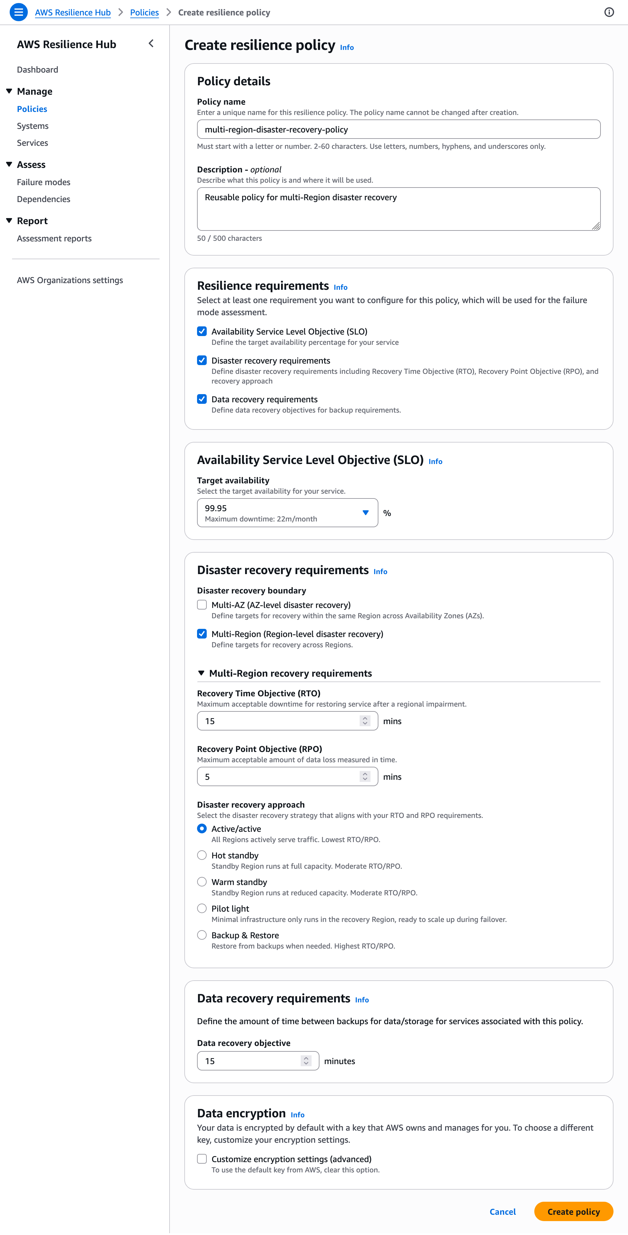
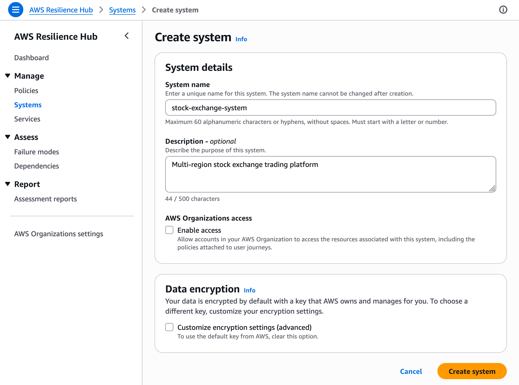
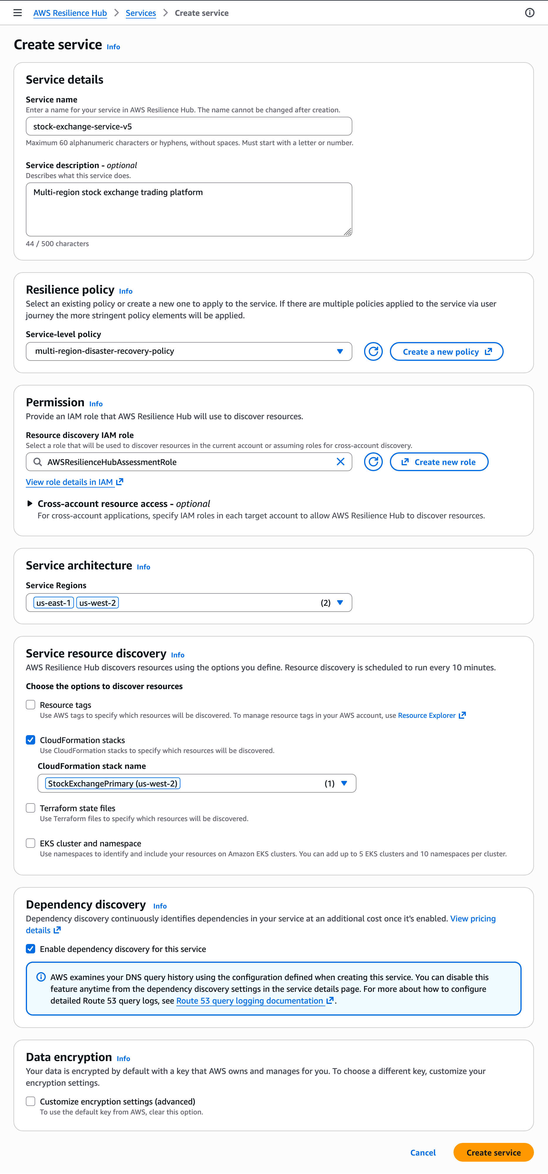
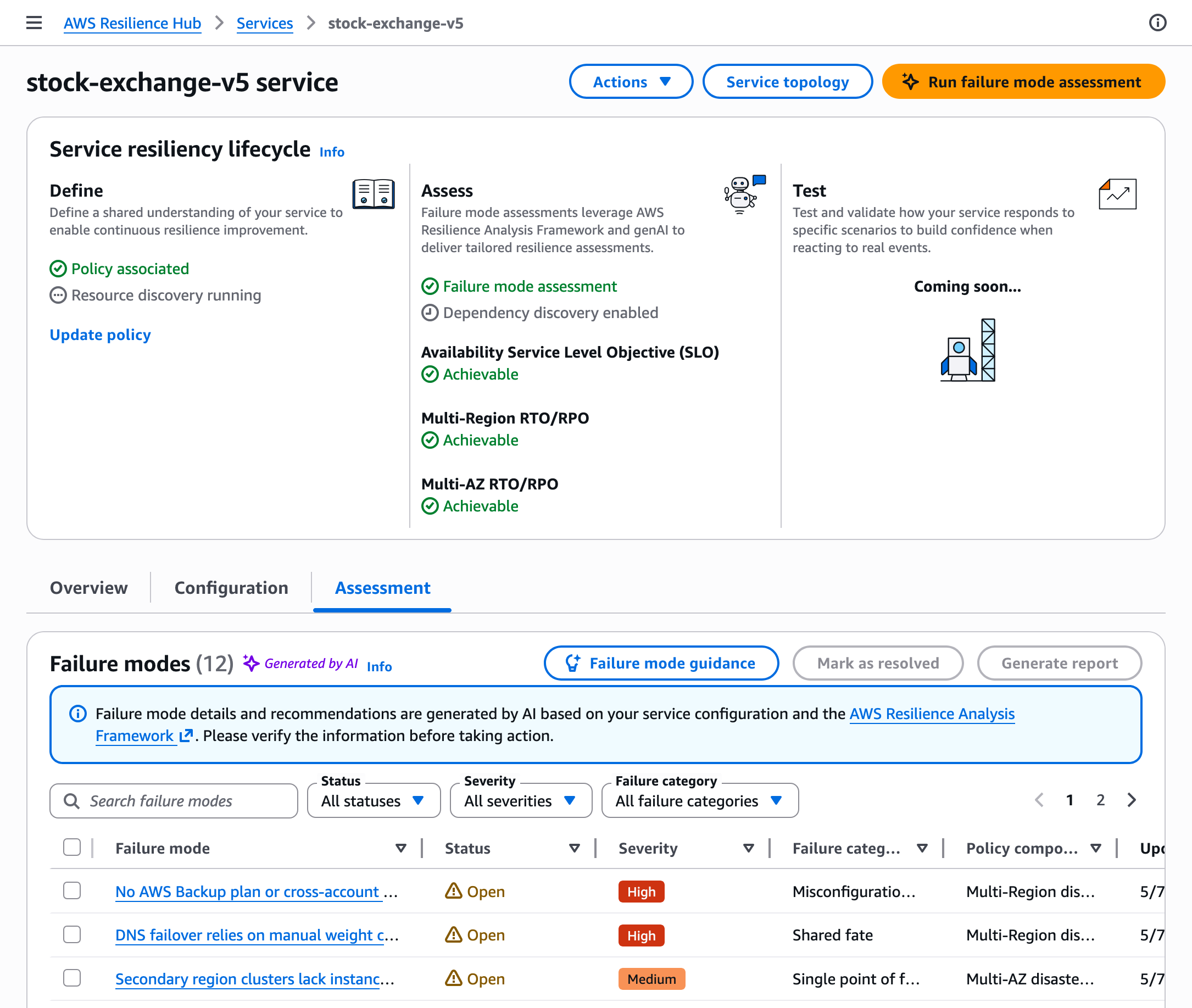
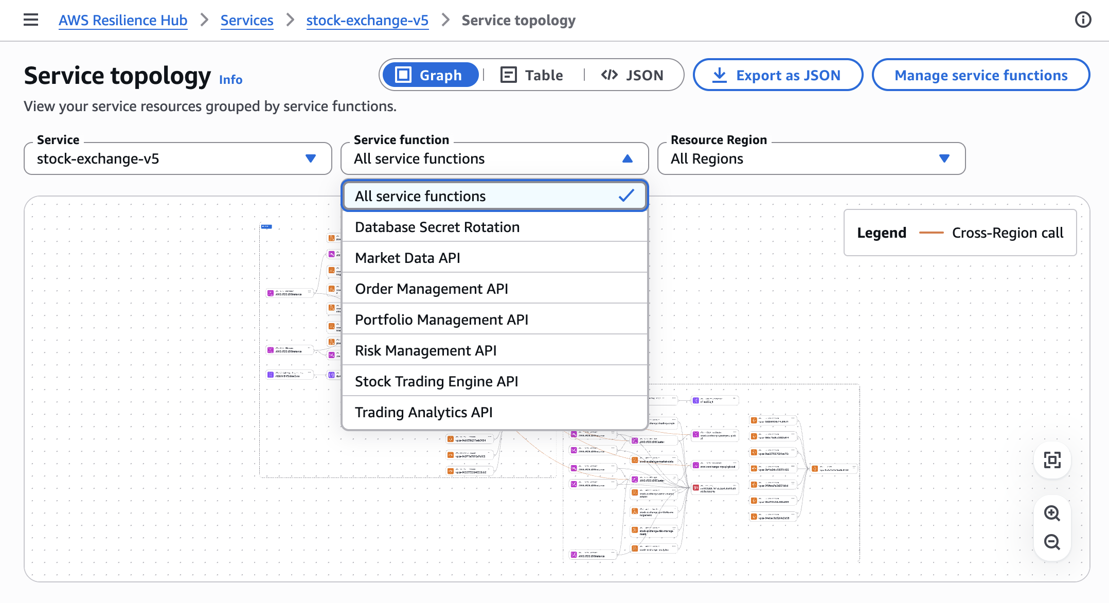

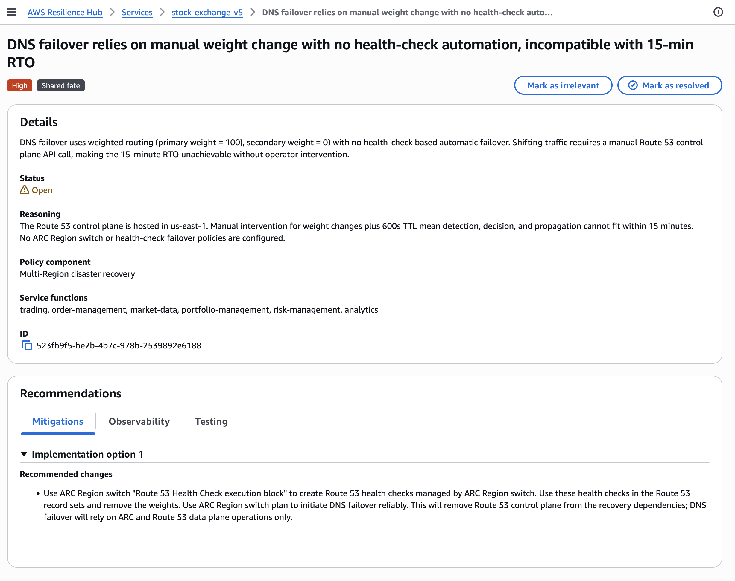
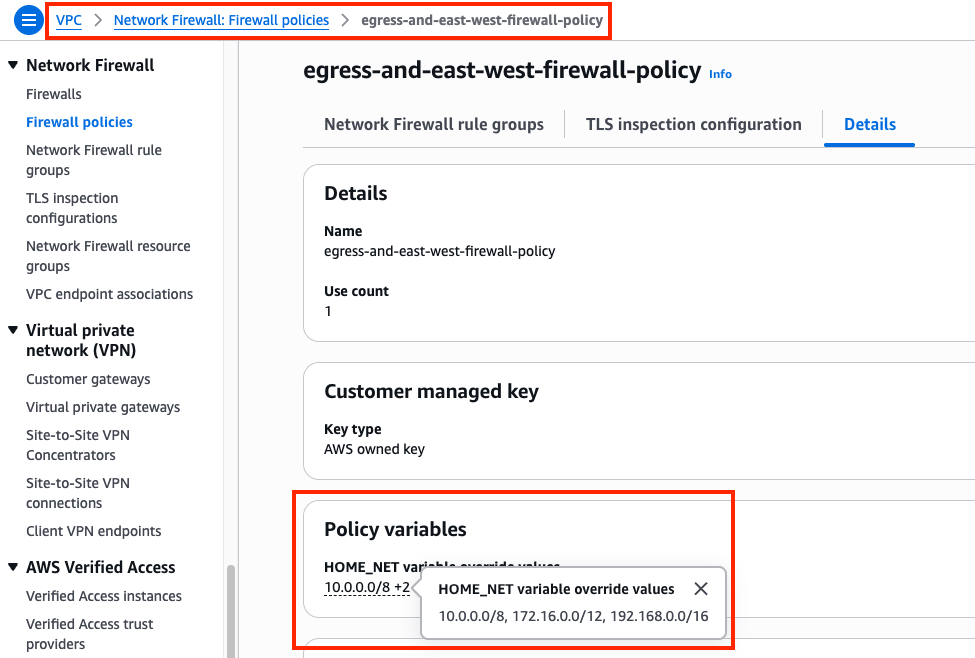
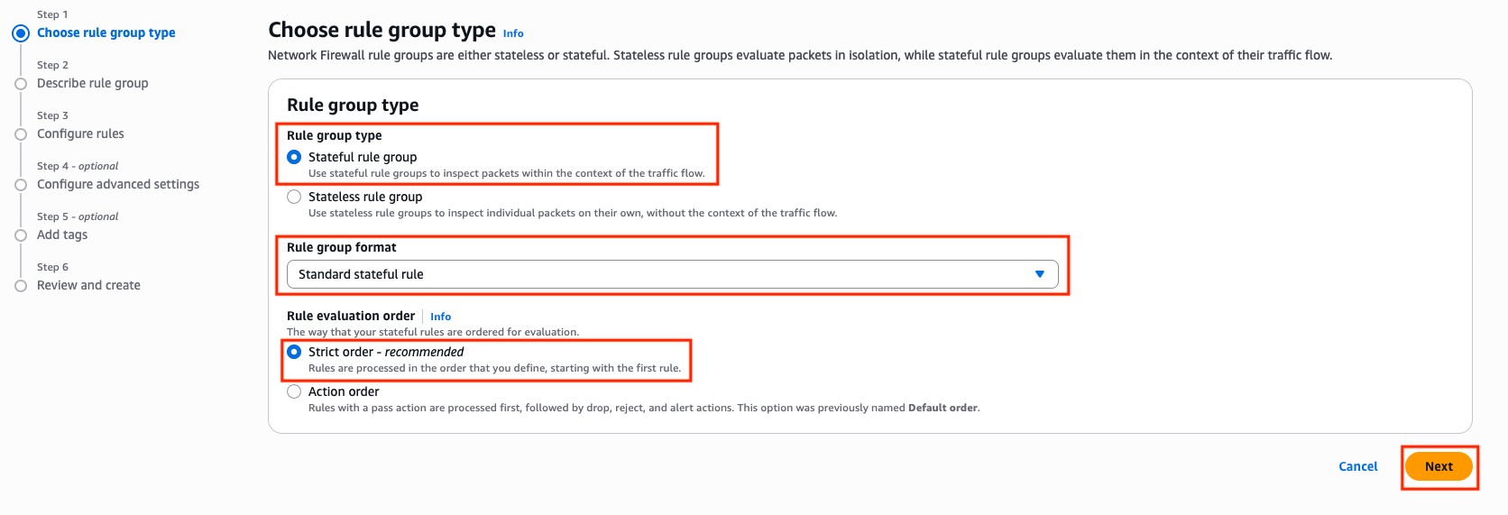
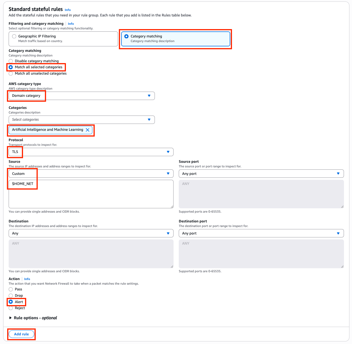
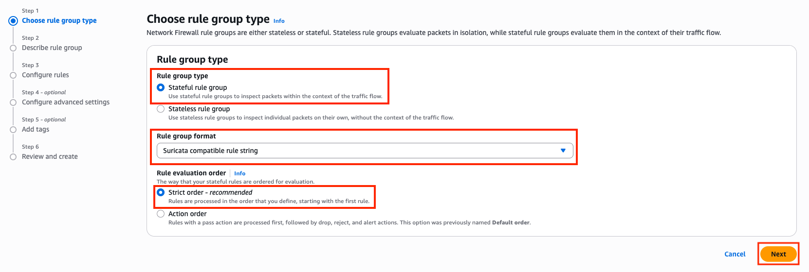
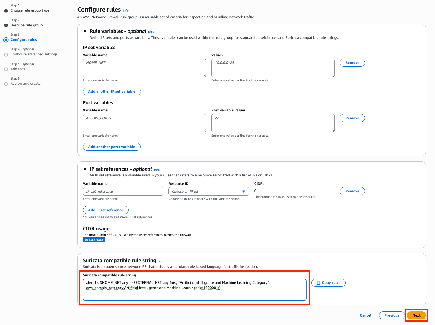
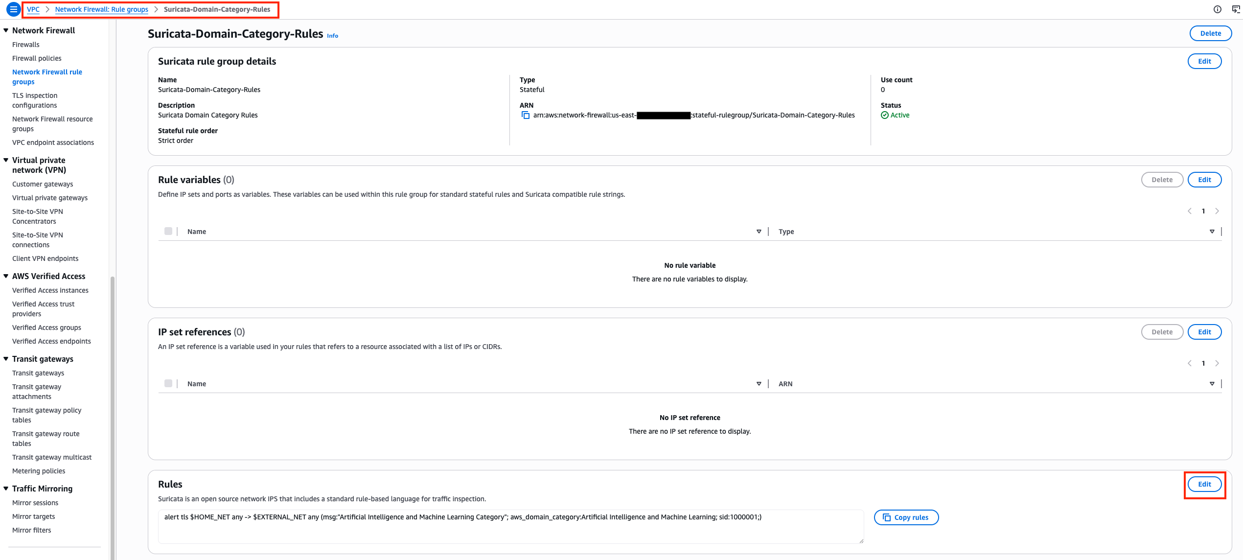
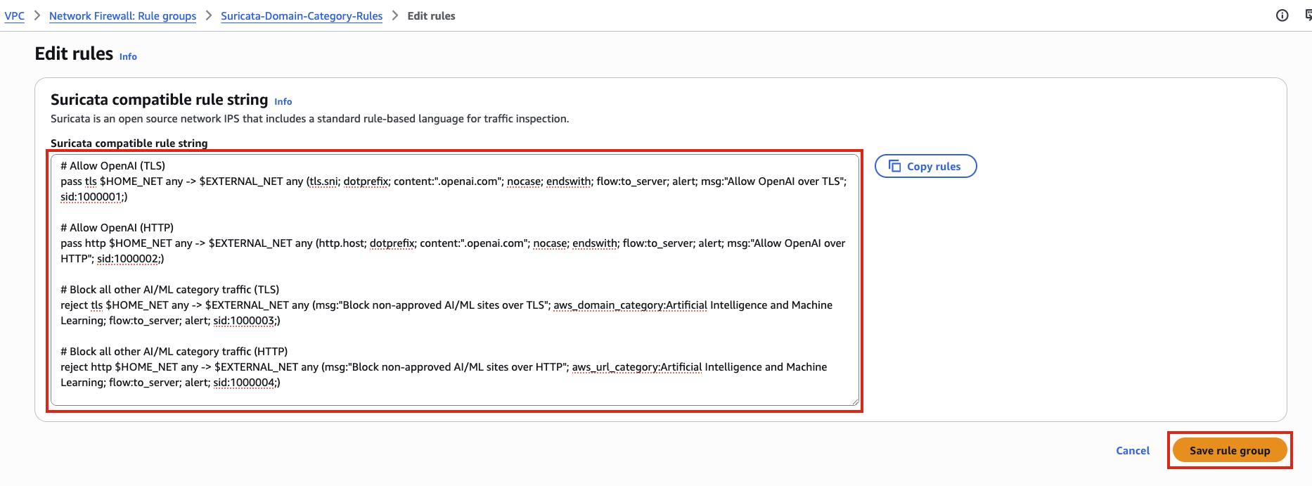
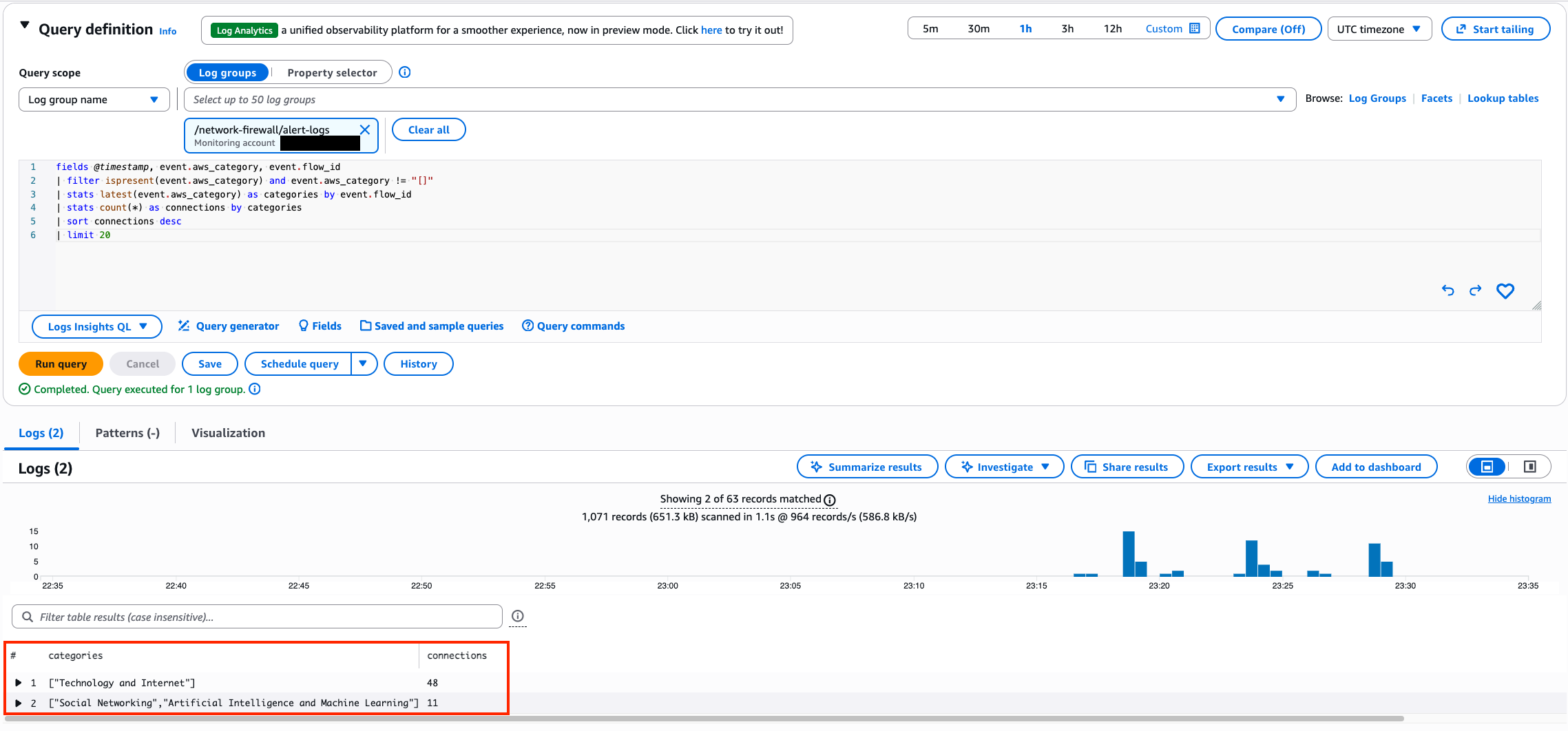
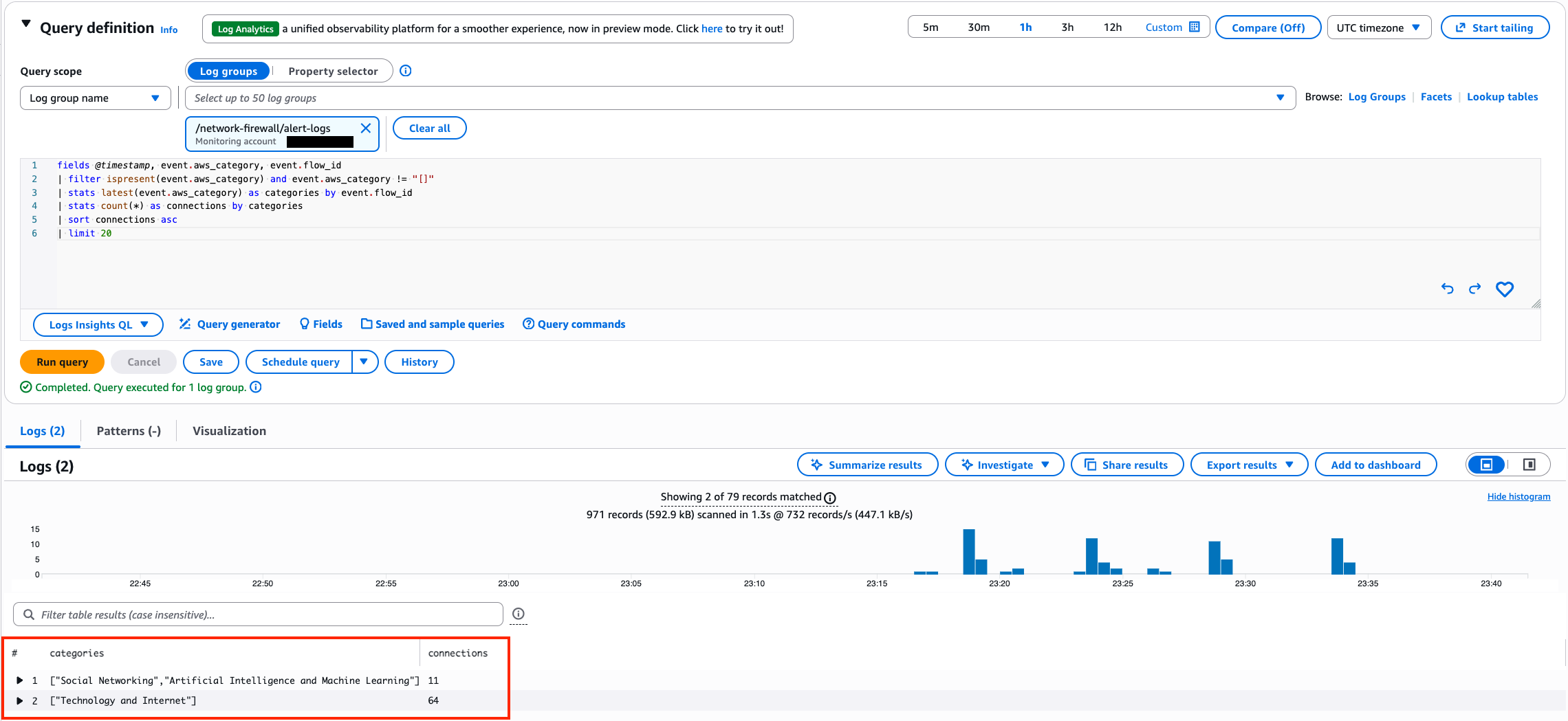
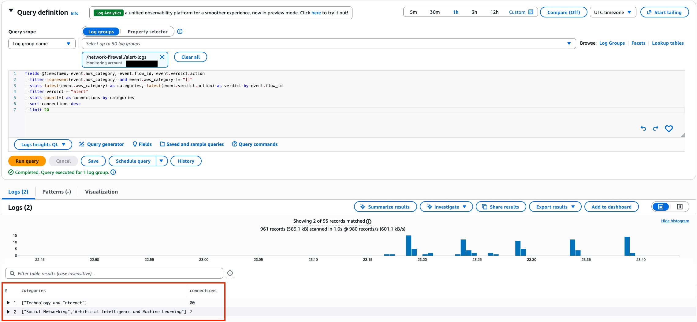
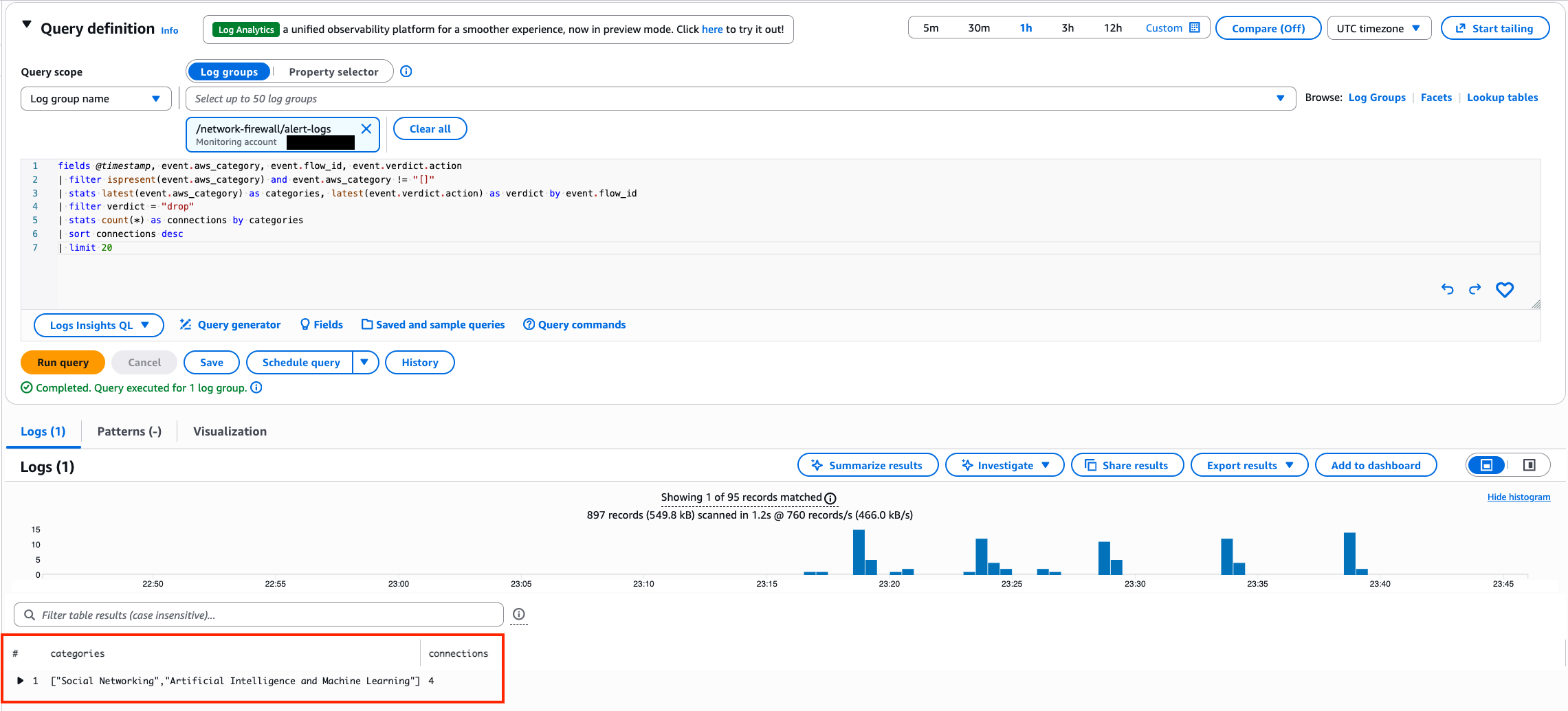
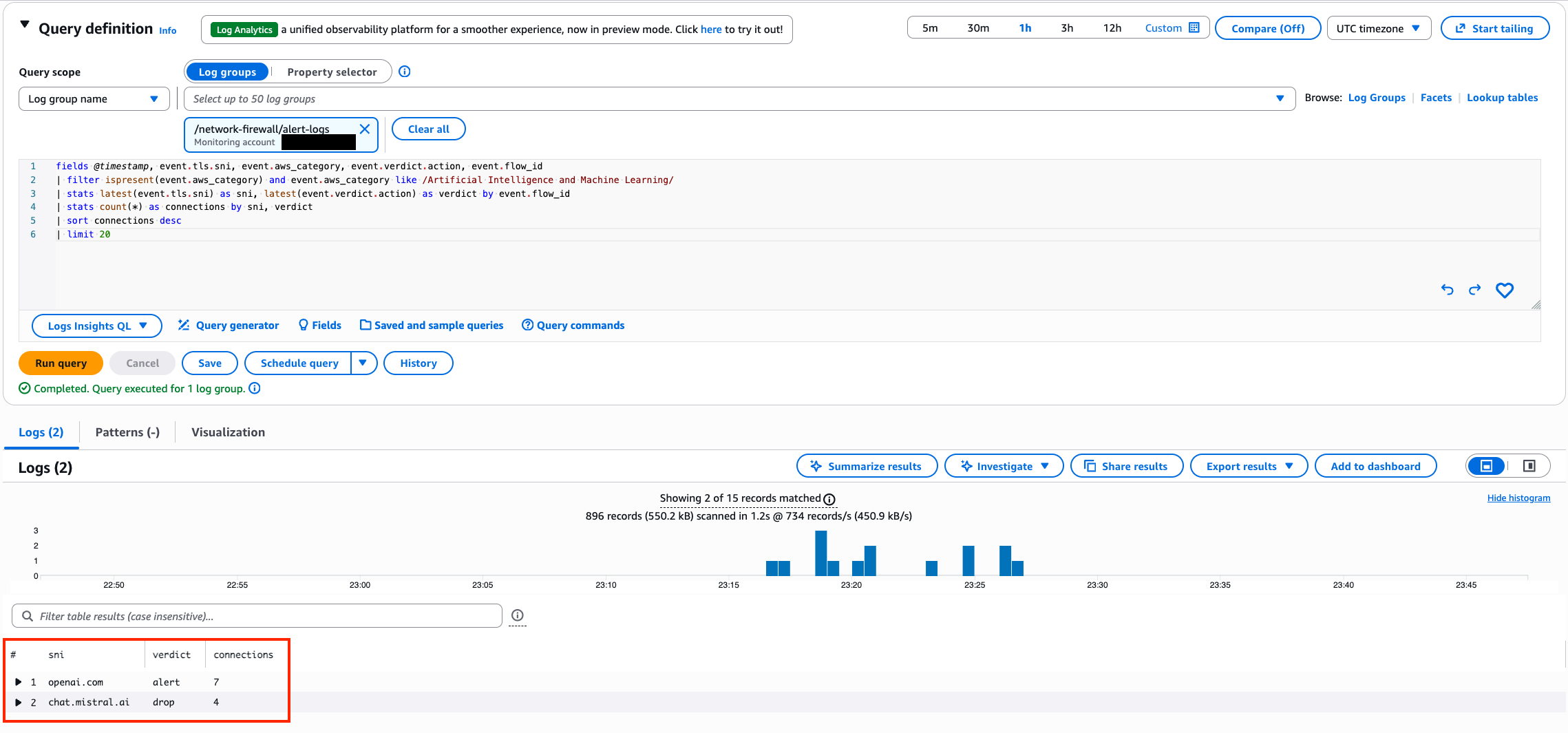
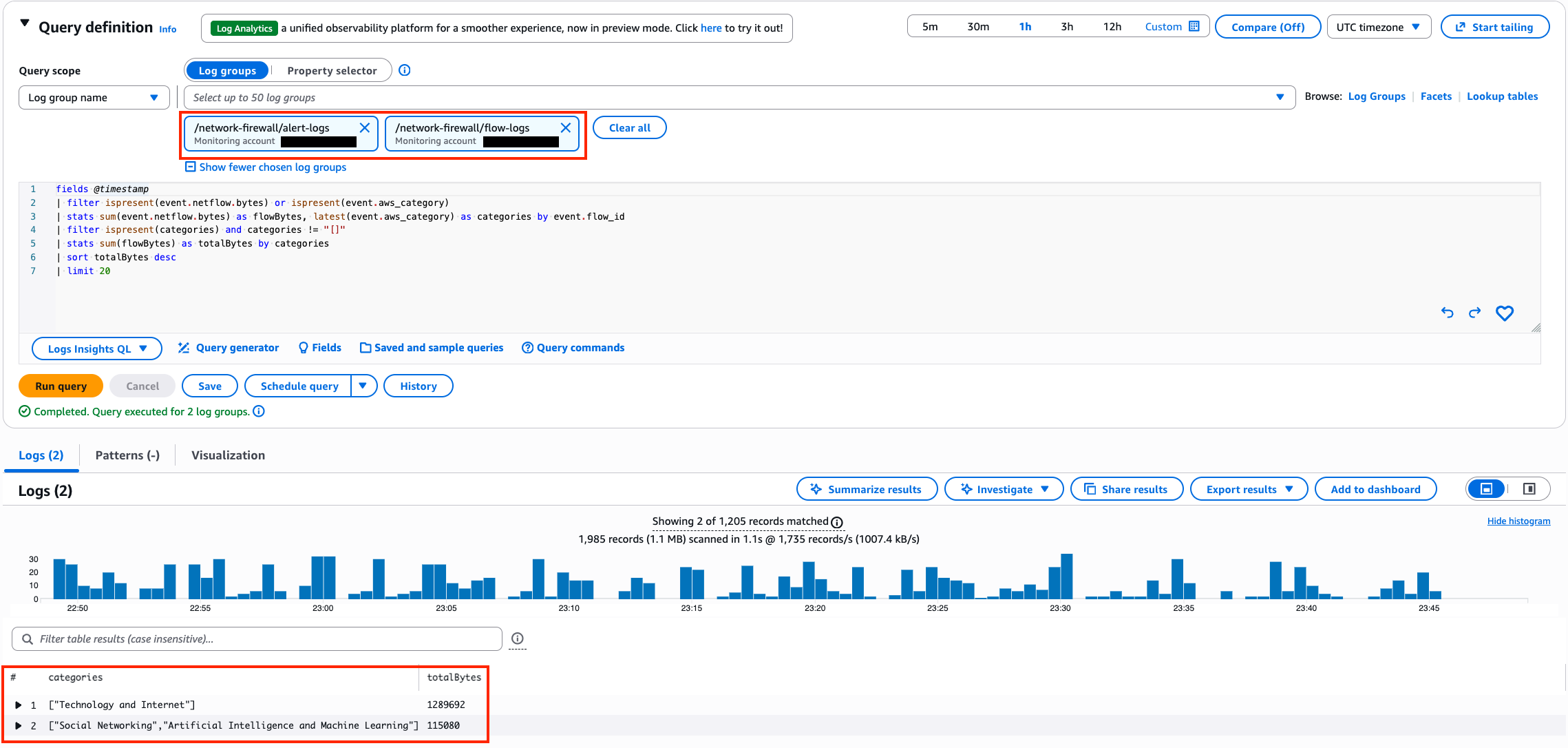
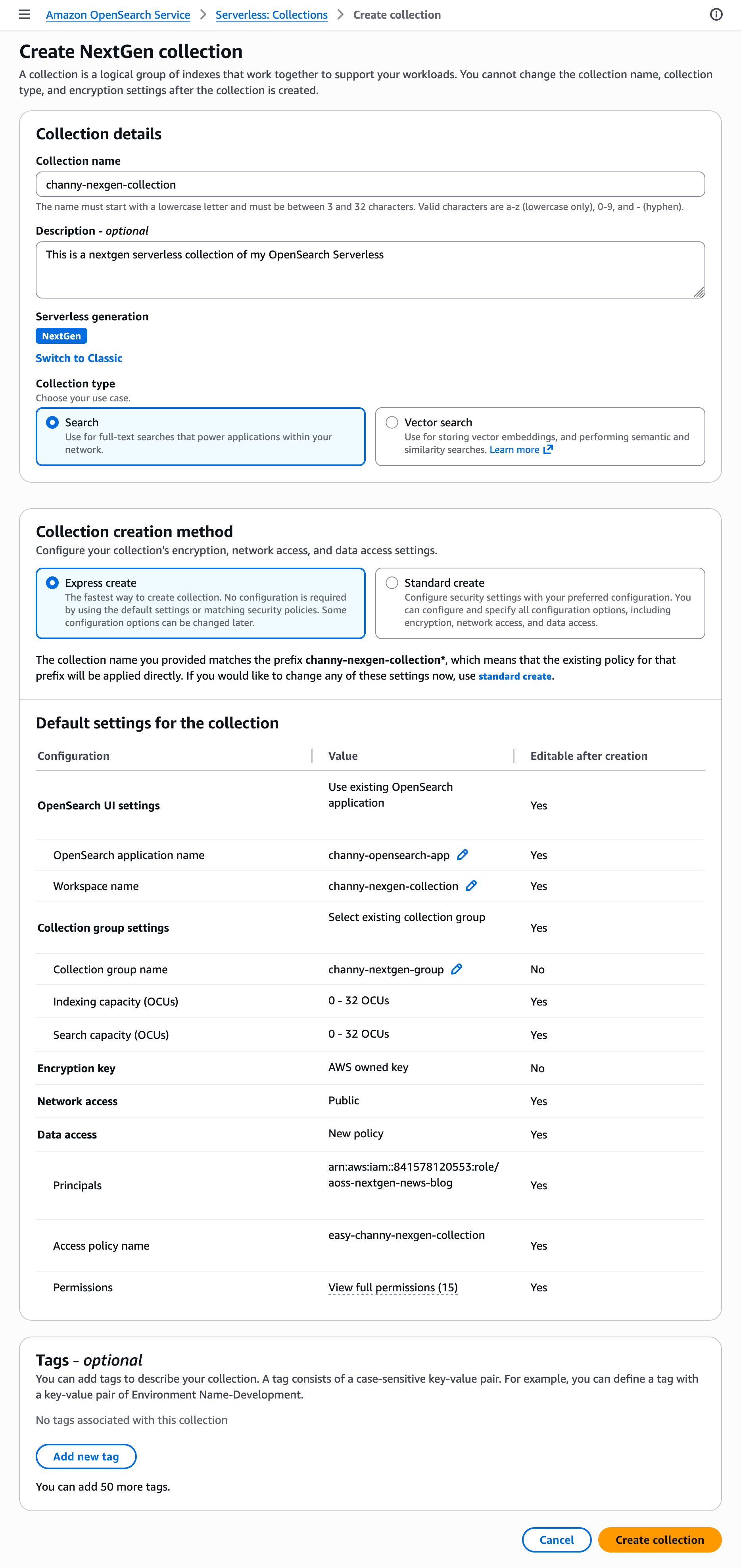
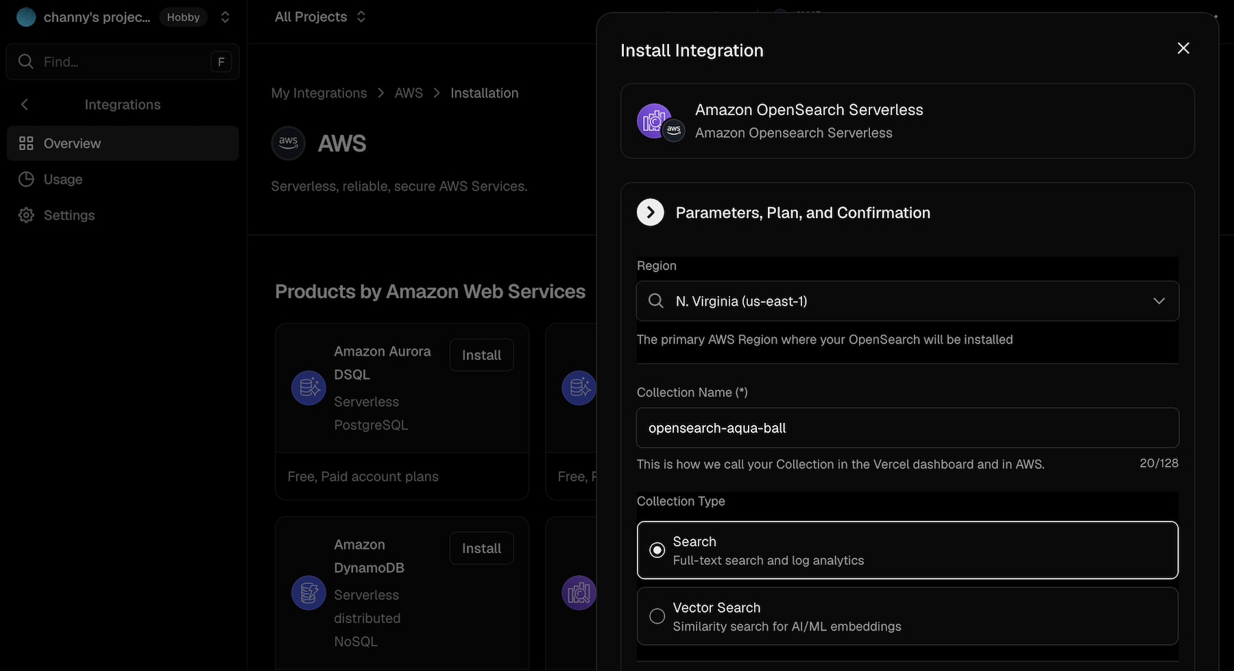
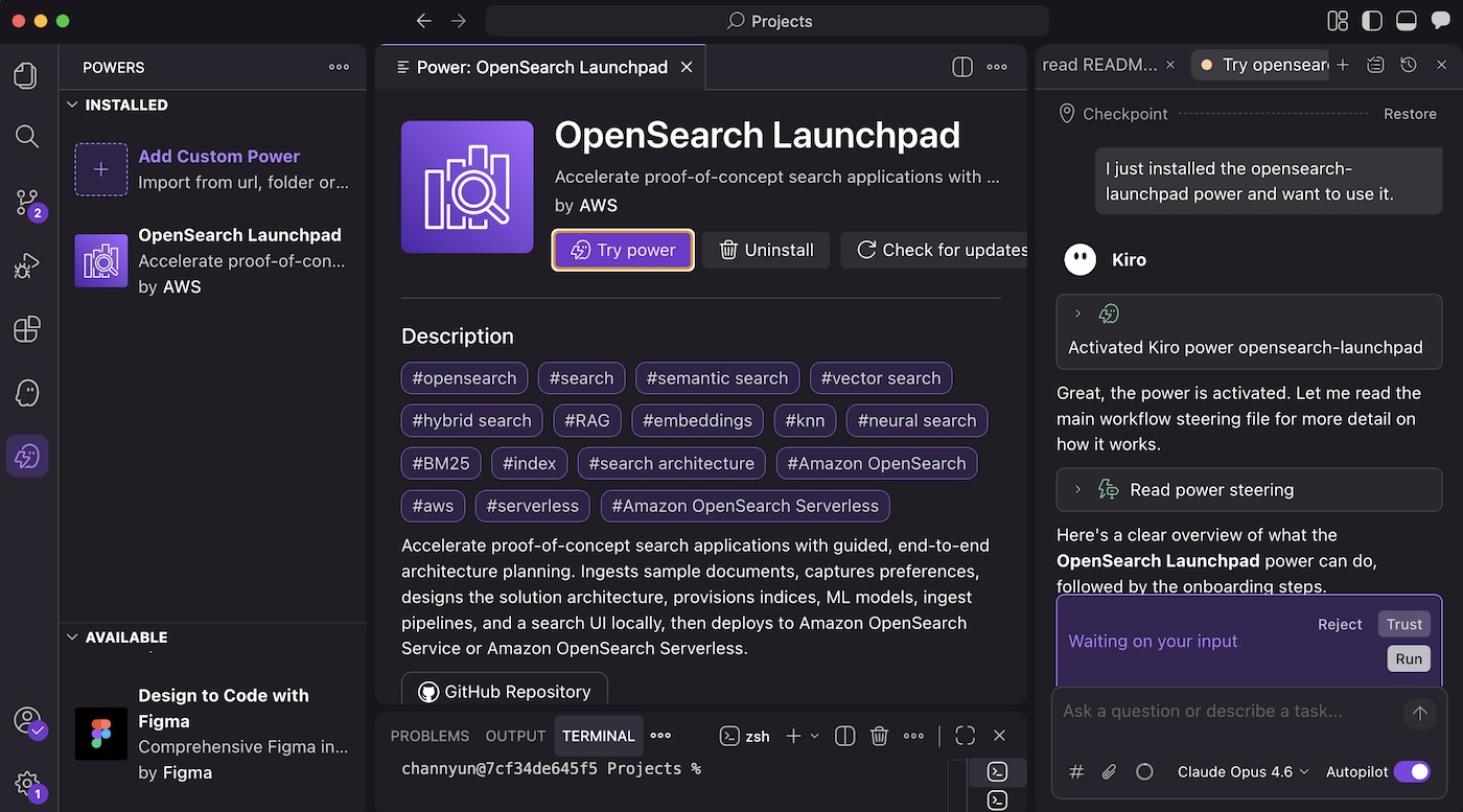
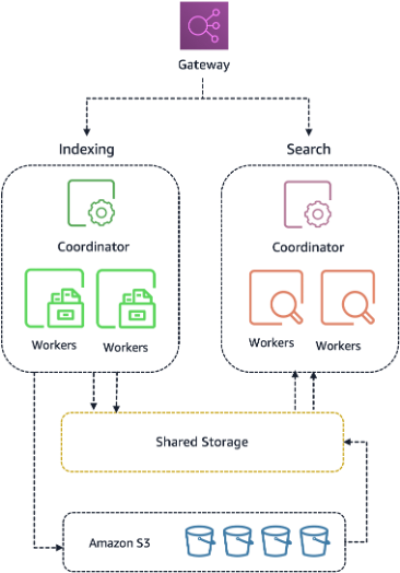
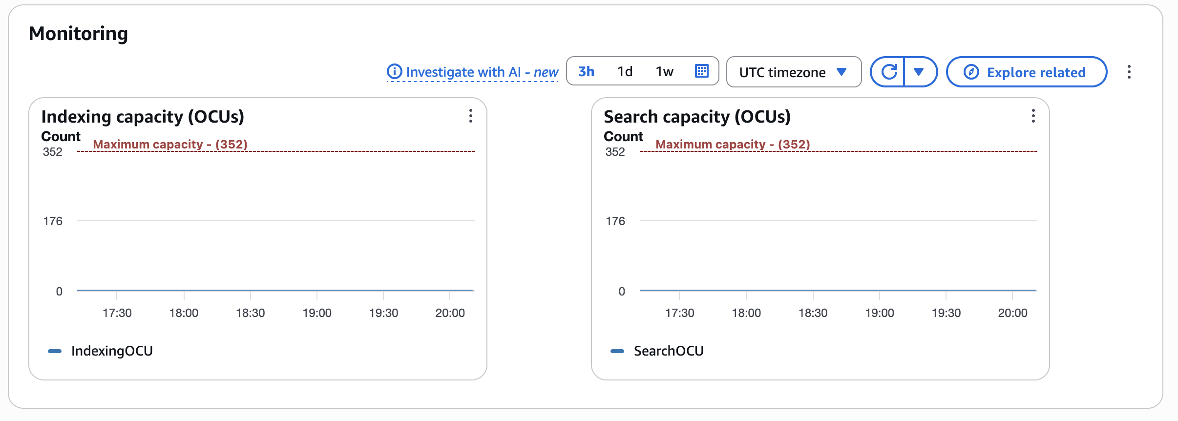


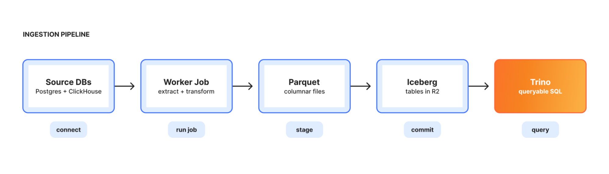
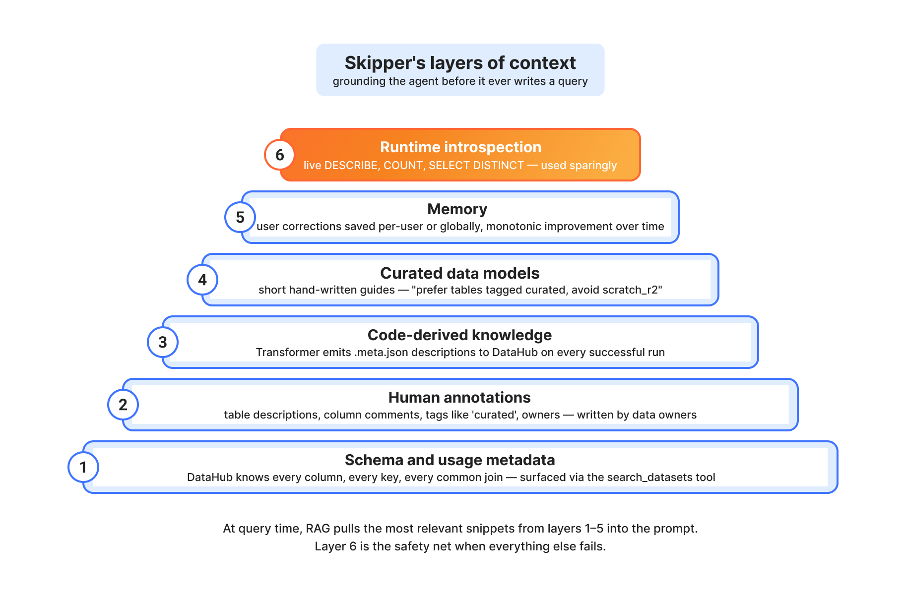


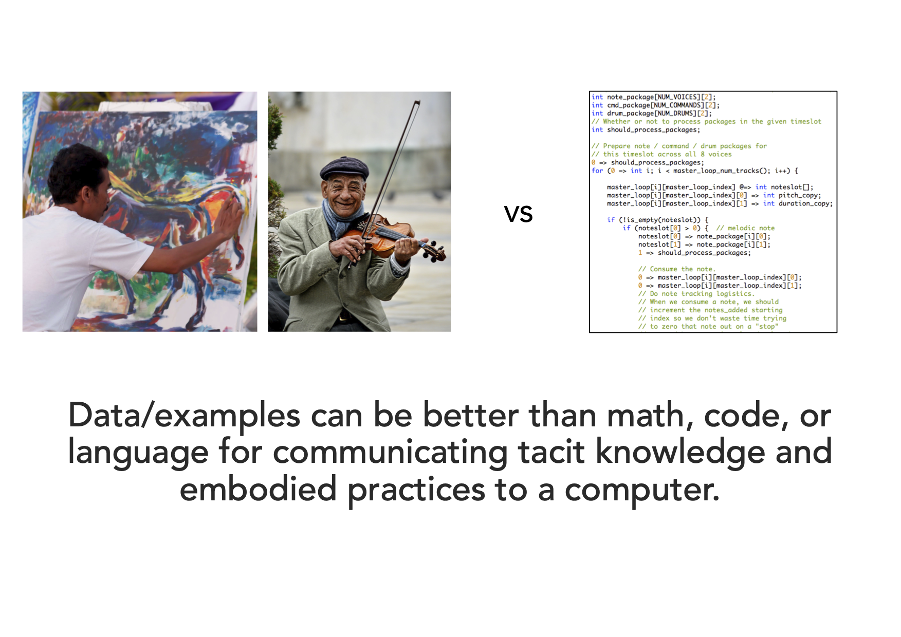
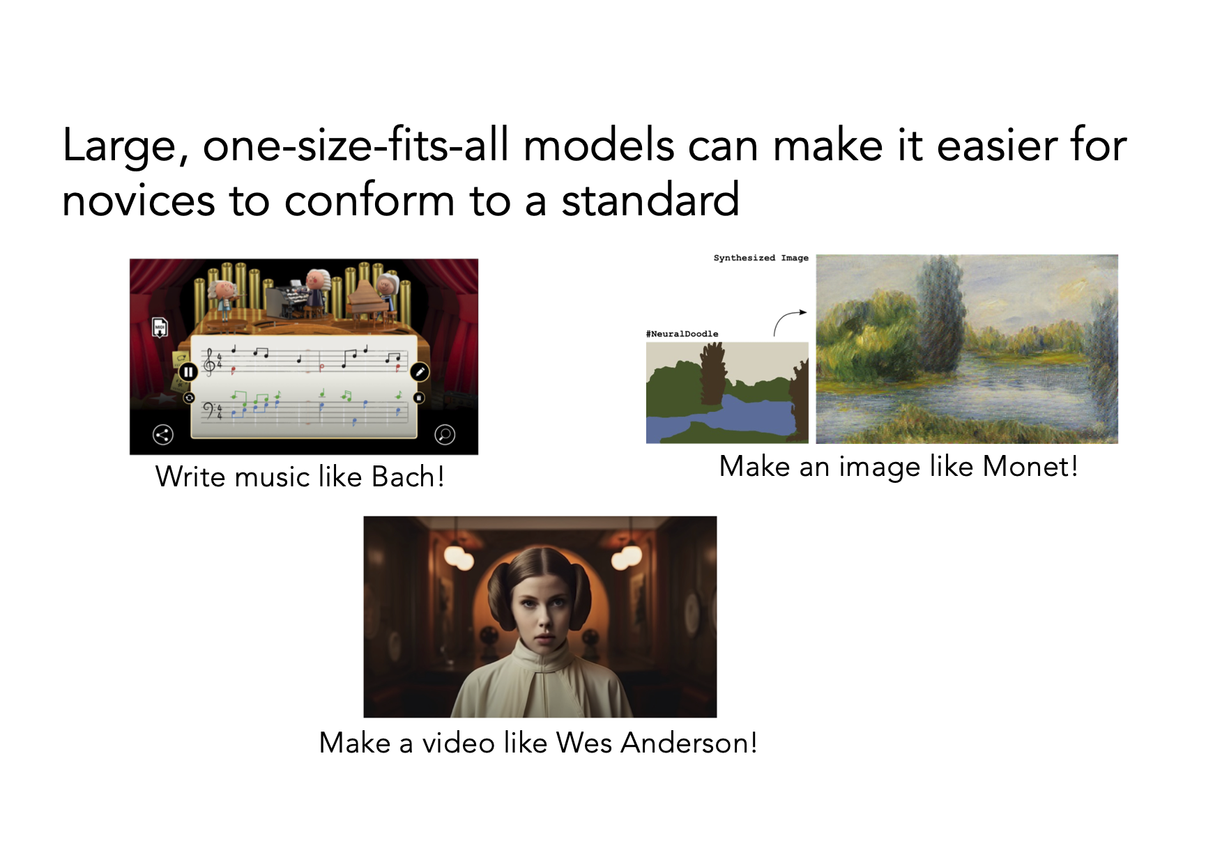
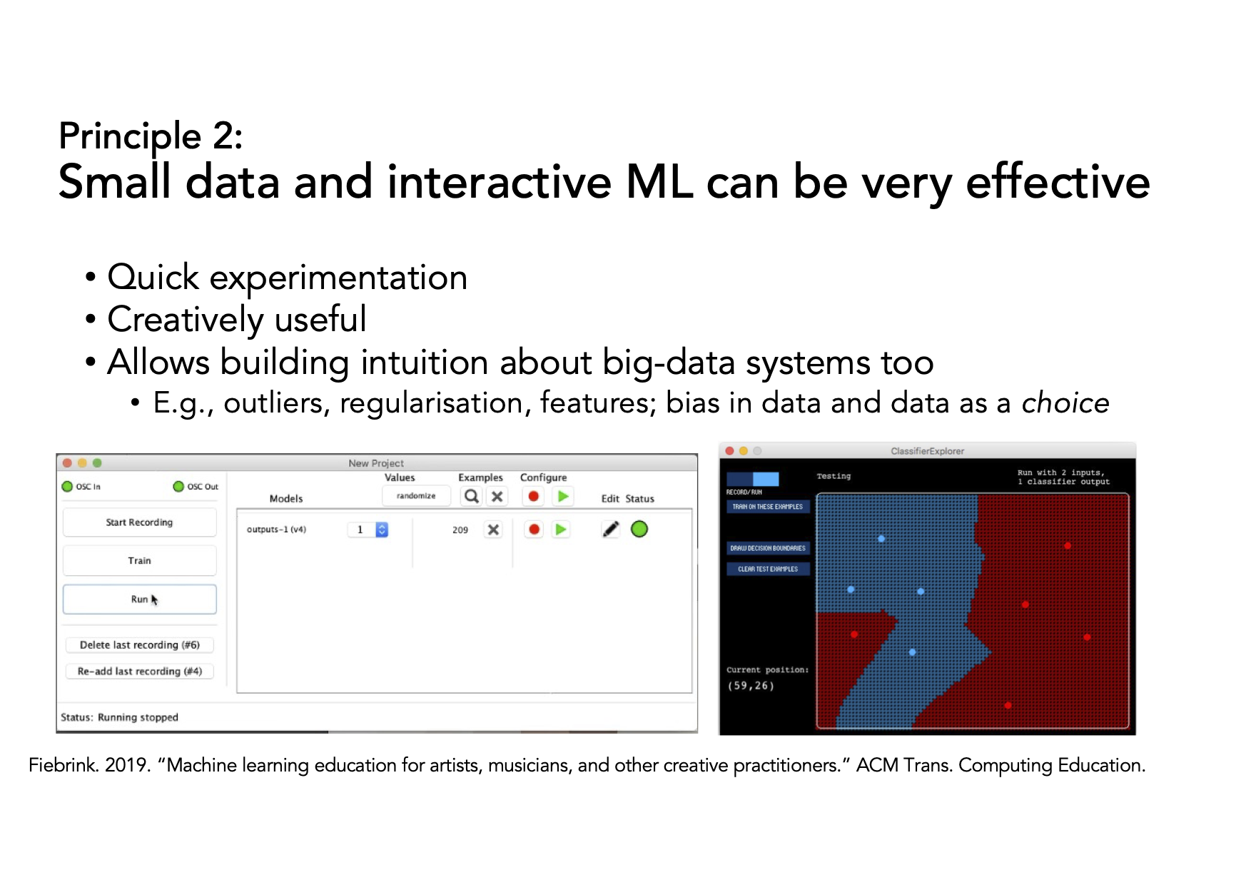
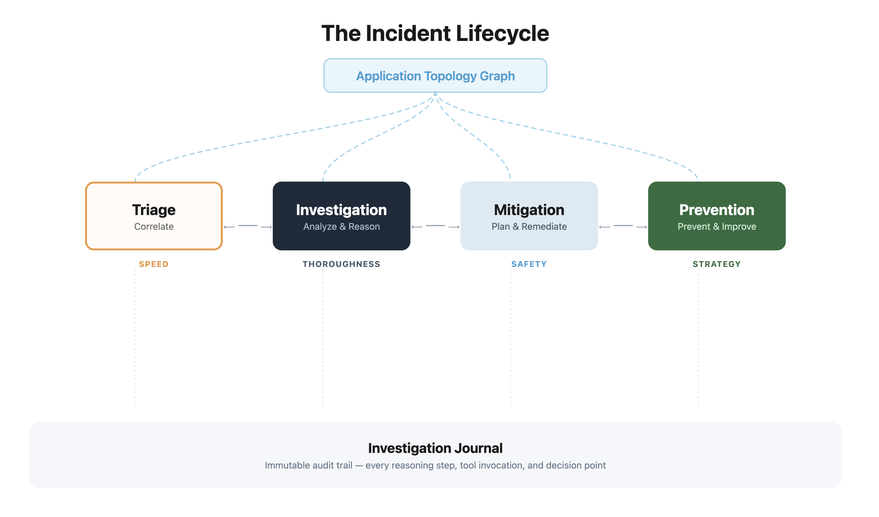
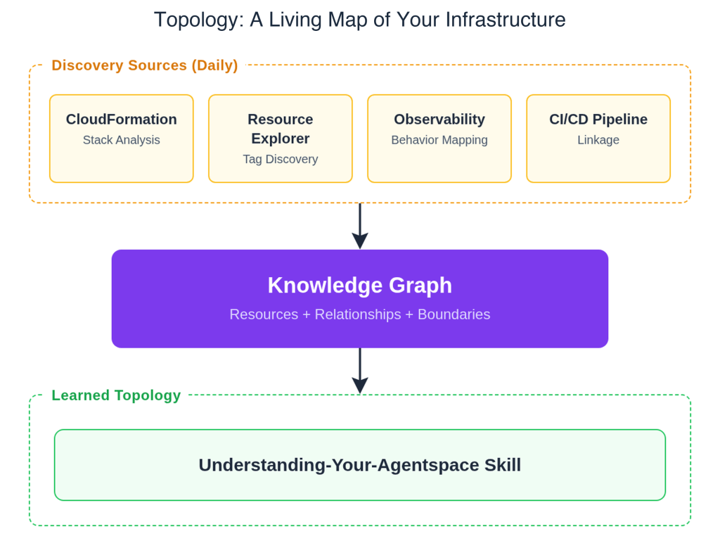
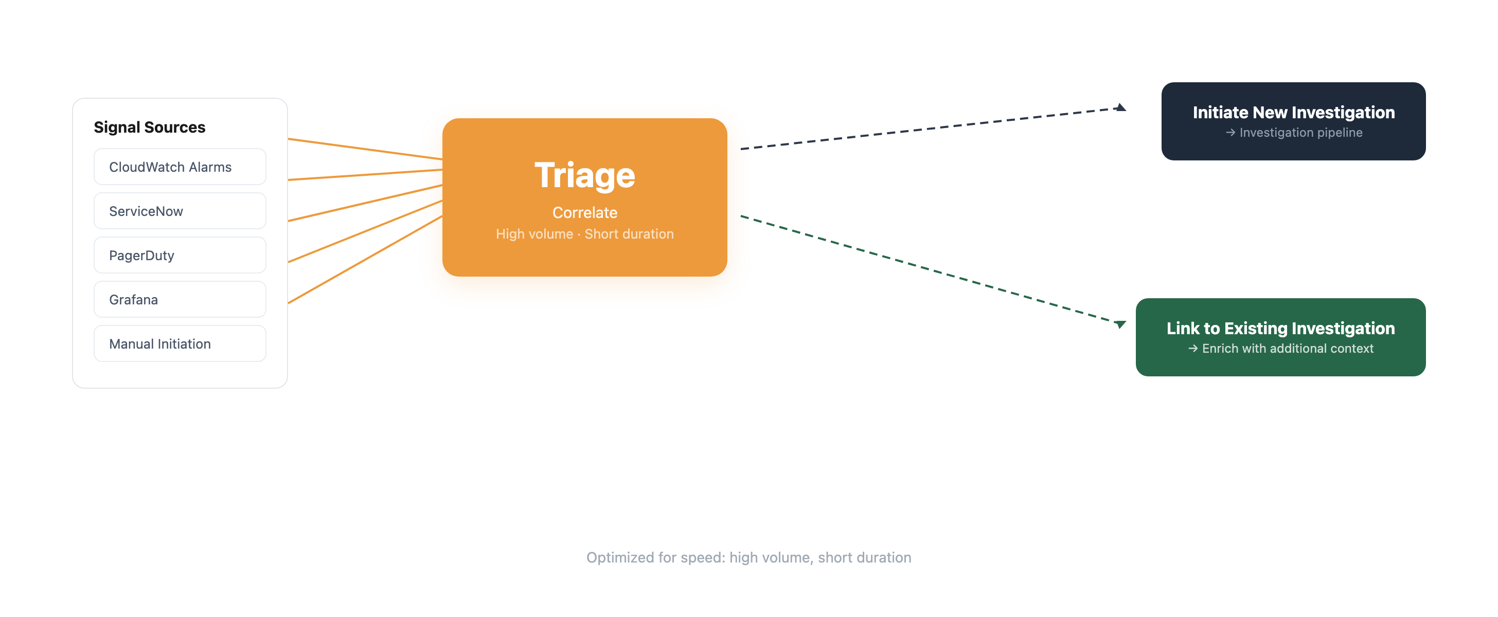 Triage is optimized for speed — high volume, short duration. It correlates incoming signals with related alerts and enriches investigations with correlation context.
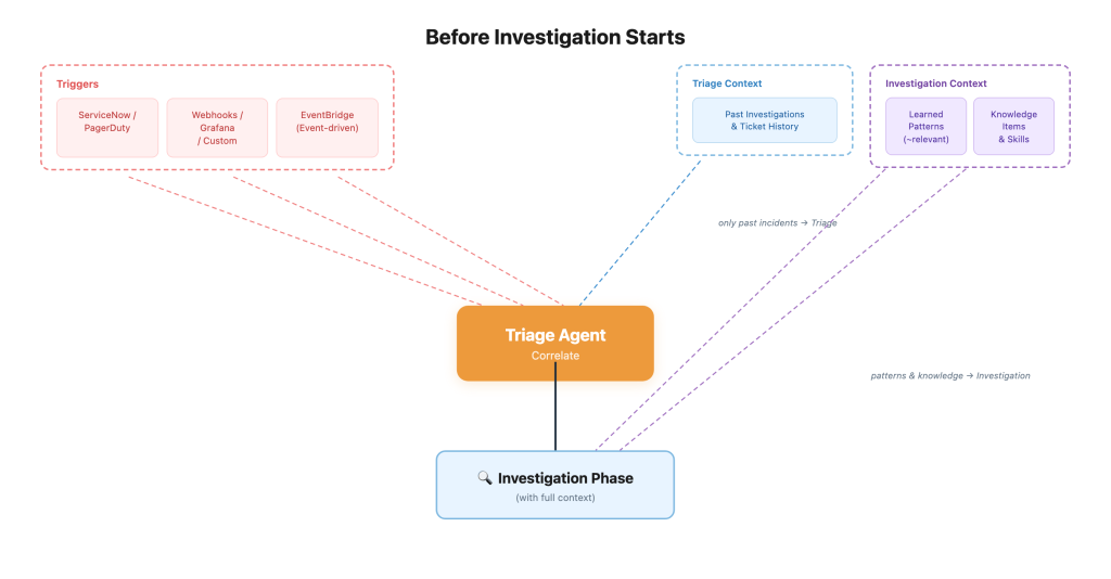
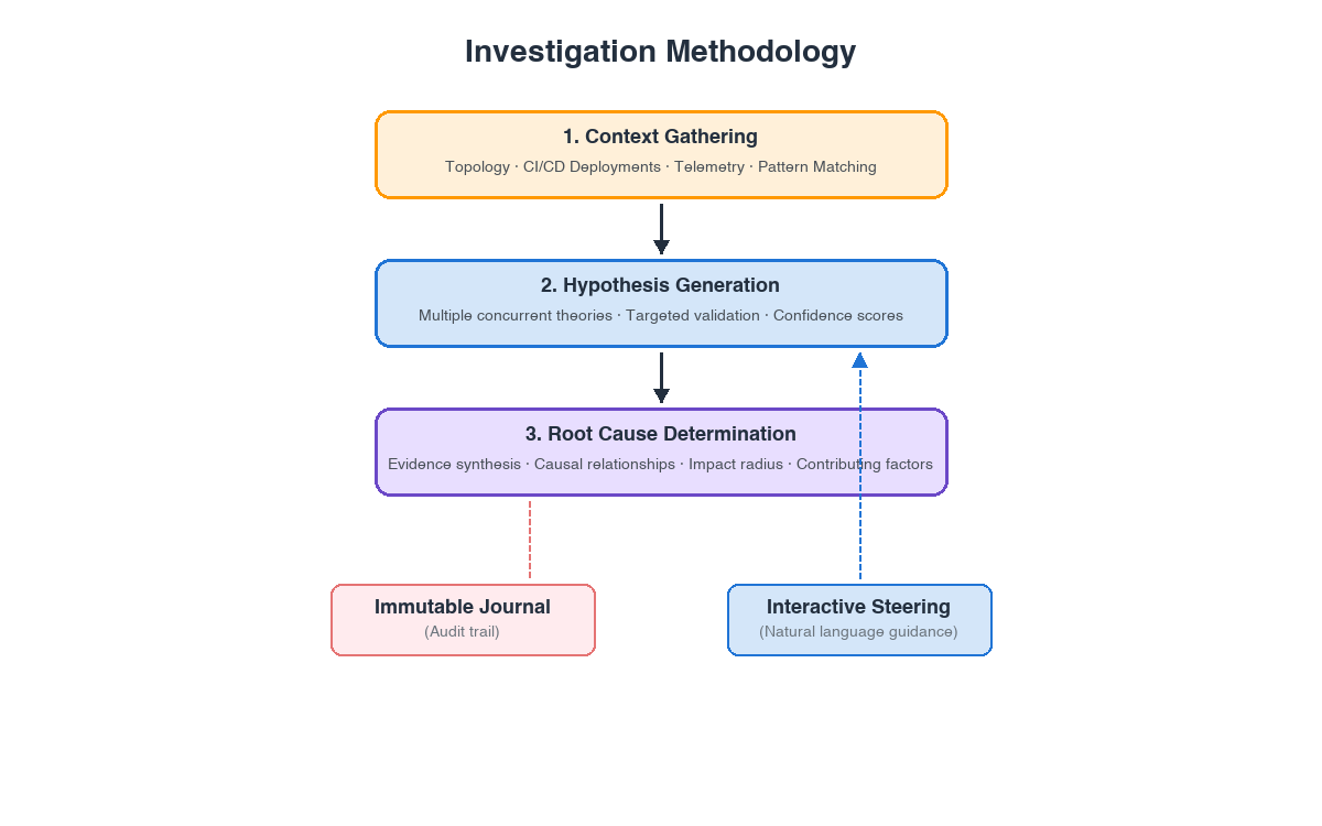 The agent pursues multiple hypotheses simultaneously, validating each with both supporting evidence and counter-evidence before surfacing them to operators. As the agent builds the causal chain, it classifies validated hypotheses as either a ’cause’ or ‘root cause’ based on their connection to the incident, and labels unconnected findings as hypothesis.