Intel Manufacturing Gets its Own Profit and Loss Potentially Gearing Up for a Spin-Off

Post Syndicated from Patrick Kennedy original https://www.servethehome.com/intel-manufacturing-gets-its-own-profit-and-loss-potentially-gearing-up-for-a-spin-off/

Intel is giving its manufacturing arm its own P&L to help drive cost reductions. The announcement feels a lot like it is gearing for a split

The post Intel Manufacturing Gets its Own Profit and Loss Potentially Gearing Up for a Spin-Off appeared first on ServeTheHome.

Accelerate onboarding and seamless integration with ThoughtSpot using Amazon Redshift partner integration

Post Syndicated from Antony Prasad Thevaraj original https://aws.amazon.com/blogs/big-data/accelerate-onboarding-and-seamless-integration-with-thoughtspot-using-amazon-redshift-partner-integration/

Amazon Redshift is a fast, petabyte-scale cloud data warehouse that makes it simple and cost-effective to analyze all of your data using standard SQL. Tens of thousands of customers today rely on Amazon Redshift to analyze exabytes of data and run complex analytical queries, making it the most widely used cloud data warehouse. You can run and scale analytics in seconds on all your data without having to manage your data warehouse infrastructure.

Today, we are excited to announce ThoughtSpot as a new BI partner available through Amazon Redshift partner integration. You can onboard with ThoughtSpot in minutes directly from the Amazon Redshift console and gain faster data-driven insights. Businesses typically look at ways to derive business insights. This is where modern analytics providers such as ThoughtSpot provide value. With its powerful AI-based search, live visualizations, and developer tools and APIs for sharing embedded analytics, ThoughtSpot democratizes access to data by providing self-service tools for all users.

In this post, you will learn how to integrate seamlessly with ThoughtSpot from the Amazon Redshift console. With the loosely coupled nature of the modern data stack, it’s simple to connect Amazon Redshift with ThoughtSpot. No data movement or replication is required.

ThoughtSpot: Live analytics for your modern data stack

Static dashboards cannot deliver consistent and reliable insights at the speed and global scale that customers demand. They lack the following:

  • Opportunities for collaboration
  • Discovery and reusability
  • Secure remote data and insight access
  • Rapid use case development with single-touch insight provisioning

ThoughtSpot empowers everyone to create, consume, and operationalize data-driven insights. ThoughtSpot consumer-grade search and AI technology delivers true self-service analytics that anyone can use, while its developer-friendly platform ThoughtSpot Everywhere makes it easy to build interactive data apps that integrate with your existing cloud provider.

As organizations increasingly move to the cloud, ThoughtSpot helps them quickly unlock value from their investment. ThoughtSpot’s simple search functionality enables you to easily ask and answer data questions in seconds to unearth impactful insights directly in Amazon Redshift. ThoughtSpot for AWS provides enterprises with more freedom and flexibility by eliminating the need to move data between cloud sources so that businesses can immediately benefit from data-driven decision-making.

ThoughtSpot is an AWS Data and Analytics Competency Partner with the Amazon Redshift Ready product designation. ThoughtSpot is also part of the Powered by Amazon Redshift program.

Integrate ThoughtSpot using Amazon Redshift partner integration

Complete the following steps to integrate ThoughtSpot with Amazon Redshift:

  1. On the Amazon Redshift console, choose Clusters in the navigation pane.
  2. Select your cluster and on the Actions menu, choose Add AWS Partner integration.

Alternatively, you can choose your individual cluster and on its details page, choose Add partner integration.

  1. Select ThoughtSpot as your desired BI partner.
  2. Choose Next.

  1. Choose Add partner.

  1. Log in on the ThoughtSpot landing page.

  1. Select Continue to Setup.

  1. On the Amazon Redshift connection details page, enter your Amazon Redshift database password for Password.
  2. Choose Continue.

To connect to your Amazon Redshift cluster, make sure to enable the Publicly accessible option and allow list the ThoughtSpot IP in your Amazon Redshift cluster’s security group.

  1. Select your desired tables and choose Update.
  2. If a prompt appears, choose Update again.

After you have successfully integrated with ThoughtSpot, you will see an Active status in the Integrations section on the Amazon Redshift console.

Congratulations! You’re now ready to start visualizing data using ThoughtSpot. The following example shows you trends in sales growth YTD, current sales trends across regions, and a comparison between product type sales between the current year and the previous year. You can slice and dice the dataset based on the granularity defined by the user.

Partner feedback

“ThoughtSpot is thrilled to expand our long-time cooperation with AWS with the announcement of our Amazon Redshift partner integration. Leading organizations are already extracting value from their data using AI-powered analytics on Amazon Redshift, and today we are making it even more frictionless for Amazon Redshift users to launch ThoughtSpot’s free trial to solve real problems quickly.”

– Kuntal Vahalia, SVP of WW Partners & APAC

Conclusion

In this post, we discussed how Amazon Redshift partner integration provides a fast-onboarding experience and allows you to create valuable business insights by integrating with ThoughtSpot. ThoughtSpot enables you to unlock the value of your modern data stack by empowering your entire organization with live analytics and data search, while Amazon Redshift provides a modern data warehouse experience for you to manage analytics at scale.

If you’re an AWS Partner and would like to integrate your product into the Amazon Redshift console, contact [email protected] for additional information and guidance. This console partner integration functionality is available to new and existing customers at no additional cost. To get started and learn more, see Integrating Amazon Redshift with an AWS Partner.


About the Authors

Antony Prasad Thevaraj is a Sr. Partner Solutions Architect in Data and Analytics at AWS. He has over 12 years of experience as a Big Data Engineer, and has worked on building complex ETL and ELT pipelines for various business units.

Maneesh Sharma is a Senior Database Engineer at AWS with more than a decade of experience designing and implementing large-scale data warehouse and analytics solutions. He collaborates with various Amazon Redshift Partners and customers to drive better integration.

[$] Merging copy offload

Post Syndicated from original https://lwn.net/Articles/935260/

Kernel support for copy offload is a feature that has been floating around
in limbo for a decade or more at this point; it has been implemented along
the way, but never merged. The idea is that the host
system can simply ask a block storage device to copy some data within the device
and it
will do so without further involving the host; instead of reading data into
the host so that it can be written back out again, the device circumvents
that process. At the
2023 Linux Storage, Filesystem,
Memory-Management and BPF Summit
, Nitesh Shetty led a storage and
filesystem session to discuss the current status of a patch set that he and
others have been working on, with an
eye toward getting something merged fairly soon.

Ethical Problems in Computer Security

Post Syndicated from Bruce Schneier original https://www.schneier.com/blog/archives/2023/06/ethical-problems-in-computer-security.html

Tadayoshi Kohno, Yasemin Acar, and Wulf Loh wrote excellent paper on ethical thinking within the computer security community: “Ethical Frameworks and Computer Security Trolley Problems: Foundations for Conversation“:

Abstract: The computer security research community regularly tackles ethical questions. The field of ethics / moral philosophy has for centuries considered what it means to be “morally good” or at least “morally allowed / acceptable.” Among philosophy’s contributions are (1) frameworks for evaluating the morality of actions—including the well-established consequentialist and deontological frameworks—and (2) scenarios (like trolley problems) featuring moral dilemmas that can facilitate discussion about and intellectual inquiry into different perspectives on moral reasoning and decision-making. In a classic trolley problem, consequentialist and deontological analyses may render different opinions. In this research, we explicitly make and explore connections between moral questions in computer security research and ethics / moral philosophy through the creation and analysis of trolley problem-like computer security-themed moral dilemmas and, in doing so, we seek to contribute to conversations among security researchers about the morality of security research-related decisions. We explicitly do not seek to define what is morally right or wrong, nor do we argue for one framework over another. Indeed, the consequentialist and deontological frameworks that we center, in addition to coming to different conclusions for our scenarios, have significant limitations. Instead, by offering our scenarios and by comparing two different approaches to ethics, we strive to contribute to how the computer security research field considers and converses about ethical questions, especially when there are different perspectives on what is morally right or acceptable. Our vision is for this work to be broadly useful to the computer security community, including to researchers as they embark on (or choose not to embark on), conduct, and write about their research, to program committees as they evaluate submissions, and to educators as they teach about computer security and ethics.

The paper will be presented at USENIX Security.

Crafting a better, faster code view

Post Syndicated from Joshua Brown original https://github.blog/2023-06-21-crafting-a-better-faster-code-view/

Reading code is not as simple as reading the text of a file end-to-end. It is a non-linear, sometimes chaotic process of jumping between files to follow a trail, building a mental picture of how code relates to its surrounding context. GitHub’s mission is to be the home for all developers, and reading code is one of the core experiences we offer. Every day, millions of users use GitHub to view and interact with code. So, about a year ago we set out to create a new code view that supports the entire code reading experience with features like a file tree, symbol navigation, code search integration, sticky lines, and code section folding. The new code view is powerful, intelligent, and interactive, but it is not an attempt to turn the repository browsing experience into an IDE.

While building the new code view, our team had a few guiding principles on which we refused to compromise:

  • It must add these powerful new features to transform how users read code on GitHub.
  • It must be intuitive and easy to use for all of GitHub’s millions of users.
  • It must be fast.

Initial efforts

The first step was to build out the features we wanted in a natural, straightforward way, taking the advice that “premature optimization is the root of all evil.”1 After all, if simple code satisfactorily solves our problems, then we should stop there. We knew we wanted to build a highly interactive and stateful code viewing experience, so we decided to use React to enable us to iterate more quickly on the user interface. Our initial implementation for the code blob was dead-simple: our syntax highlighting service converted the raw file contents to a list of HTML strings corresponding to the lines of the file, and each of these lines was added to the document.

There was one key problem: our performance scaled badly with the number of lines in the file. In particular, our LCP and TTI times measurably increased at around 500 lines, and this increase became noticeable at around 2,000 lines. Around those same thresholds, interactions like highlighting a line or collapsing a code section became similarly sluggish. We take these performance metrics seriously for a number of reasons. Most importantly, they are user-centric—that is, they are meant to measure aspects of the quality of a user’s experience on the page. On top of that, they are also part of how search engines like Google determine where to rank pages in their search results; fast pages get shown first, and the code view is one of the many ways GitHub’s users can show their work to the world.

As we dug in, we discovered that there were a few things at play:

  • When there are many DOM nodes on the page, style calculations and paints take longer.
  • When there are many DOM nodes on the page, DOM queries take longer, and the results can have a significant memory footprint.
  • When there are many React nodes on the page, renders and DOM reconciliation both take longer.

It’s worth noting that none of these are problems with React specifically; any page with a very large DOM would experience the first two problems, and any solution where a large DOM is created and managed by JavaScript would experience the third.

We mitigated these problems considerably by ensuring that we were not running these expensive operations more than necessary. Typical React optimization techniques like memoization and debouncing user input, as well as some less common solutions like pulling in an observer pattern went a long way toward ensuring that React state updates, and therefore DOM updates, only occurred as needed.

Mitigating the problem, however, is not solving the problem. Even with all of these optimizations in place, the initial render of the page remained a fundamentally expensive operation for large files. In the repository that builds GitHub.com, for example, we have a CODEOWNERS file that is about 18,000 lines long, and pushes the 2MB size limit for displaying files in the UI. With no optimizations besides the ones described above, React’s first pass at building the DOM for this page takes nearly 27 seconds.2 Considering more than half of users will abandon a page if it loads for more than three seconds, there was obviously lots of work left to do.

A promising but incomplete solution

Enter virtualization. Virtualization is a performance optimization technique that examines the scroll state of the page to determine what content to include in the DOM. For example, if we are viewing a 10,000 line file but only about 75 lines fit on the screen at a time, we can save lots of time by only rendering the lines that fit in the viewport. As the user scrolls, we add any lines that need to appear, and remove any lines that can disappear, as illustrated by this demo.3

This satisfies the most basic requirements of the page with flying colors. It loads on average more quickly than the existing experience, and the experience of scrolling through the file is nearly indistinguishable from the non-virtualized case. Remember that 27 second initial render? Virtualizing the file content gets that time down to under a second, and that number does not increase substantially even if we artificially remove our file size limit and pull in hundreds of megabytes of text.

Unfortunately, virtualization is not a cure-all. While our initial implementation added features to the page at the expense of performance, naïvely virtualizing the code lines delivers a fast experience at the expense of vital functionality. The biggest problem was that without the entire text of the file on the page at once, the browser’s built-in find-in-file only surfaced results that are visible in the viewport. Breaking users’ ability to find text on the page breaks our hard requirement that the page remain intuitive and easy to use. Before we could ship any of this to real users, we had to ensure that this use case would be covered.

The immediate solution was to implement our own version of find-in-file by implementing a custom handler for the Ctrl+F shortcut (⌘+F on Mac). We added a new piece of UI in the sidebar to show results as part of our integration with symbol navigation and code search.

Screenshot of the "find" sidebar, showing a search bar with the term "isUn" and a list offive lines of code from the current file that contain that string, the second of which is highlighted as selected.

There is precedent for overriding this native browser feature to allow users to find text in virtualized code lines. Monaco, the text editor behind VS Code, does exactly this to solve the same problem, as do many other online code editors, including Repl.it and CodePen. Some other editors like the official Ruby playground ignore the problem altogether and accept that Ctrl+F will be partially broken within their virtualized editor.

At the time, we felt confident leaning on this precedent. These examples are applications that run in a browser window, and as users, we expect applications to implement their own controls. Writing our own way to find text on the page was a step toward making GitHub’s Code View less of a web page and more of a web application.

When we released the new code view experience as a private beta at GitHub Universe, we received clear feedback that our users think of GitHub as a page, not as an app. We tried to rework the experience to be as similar as possible to the native implementation, both in terms of user experience and performance. But ultimately, there are plenty of good reasons not to override this kind of native browser behavior.

  • Users of assistive technologies often use Ctrl+F to locate elements on a page, so restricting the scope to the contents of the file broke these workflows.
  • Users rely heavily on specific muscle memory for common actions, and we followed a deep rabbit hole to get the custom control to support all of the shortcuts used by various browsers.
  • Finally, the native browser implementation is simply faster.

Despite plenty of precedent for an overridden find experience, this user feedback drove us to dig deeper into how we could lean on the browser for something it already does well.

Virtualization has an important role to play in our final product, but it is only one piece of the puzzle.

How the pieces fit together

Our complete solution for the code view features two pieces:

  1. A textarea that contains the entire text of the raw file. The contents are accessible, keyboard-navigable, copyable, and findable, yet invisible.
  2. A virtualized, syntax-highlighted overlay. The contents are visible, yet hidden from both mouse events and the browser’s find.

Together, these pieces deliver a code view that supports the complete code reading experience with many new features. Despite the added complexity, this new experience is faster to render than the static HTML page that has displayed code on GitHub for more than a decade.

A textarea and a read-only cursor

The first half of this solution came to us from an unexpected angle.

Beyond adding functionality to the code view, we wanted to improve the code reading experience for users of assistive technologies like screen readers. The previous code view was minimally accessible; a code document was displayed as a table, which created a very surprising experience for screen reader users. A code document is not a table, but likewise it is not a paragraph of text. To support a familiar interface for interacting with the code on the page, we added an invisible textarea underneath the virtualized, syntax-highlighted code lines so that users can move through the code with the keyboard in a familiar way. And for the browser, rendering a textarea is much simpler than using JavaScript to insert syntax-highlighted HTML. Browsers can render megabytes of text in a textarea with ease.

Since this textarea contains the entire text of the raw file, it is not just an accessibility feature, but an opportunity to remove our custom implementation of Ctrl+F in favor of native browser implementations.

Hiding text from Ctrl+F

With the addition of the textarea, we now have two copies of every line that is visible in the viewport: one in the textarea, and another in the virtualized, syntax-highlighted overlay. In this state, searching for text yields duplicated results, which is more confusing than a slow or unfamiliar experience.

The question, then, is how to expose only one copy of the text to the browser’s native Ctrl+F. That brings us to the next key part of our solution: how we hid the syntax-highlighted overlay from find.

For a code snippet like this line of Python:

print("Hello!")

the old code view created a bit of HTML that looks like this:

<span class="pl-en">print</span>(<span class="pl-s">"Hello!"</span>)

But the text nodes containing print, (,"Hello!", and ) are all findable. It took two iterations to arrive at a format that looks identical but is consistently hidden fromCtrl+F on all major browsers. And as it turns out, this is not a question that is very easy to research!

The first approach we tried relied on the fact that :before pseudoelements are not part of the DOM, and therefore do not appear in find results. With a bit of a change to our HTML format that moves all text into a data- attribute, we can use CSS to inject the code text into the page without any findable text nodes.

HTML

<span class="pl-en" data-code-text="print"></span>
<span data-code-text="("></span>
<span class="pl-s" data-code-text=""Hello!""></span>
<span data-code-text=")"></span>

CSS

[data-code-text]:before {
   content: attr(data-code-text);
}

But that’s not the end of the story, because the major browsers do not agree on whether text in :before pseudoelements should be findable; Firefox in particular has a powerful Ctrl+F implementation that is not fooled by our first trick.

Our second attempt relied on a fact on which all browsers seem to agree: that text in adjacent pseudoelements is not treated as a contiguous block of text.4 So, even though Firefox would find print in the first example, it would not find print(. The solution, then, is to break up the text character-by-character:

<span class="pl-en">
   <span data-code-text="p"></span>
   <span data-code-text="r"></span>
   <span data-code-text="i"></span>
   <span data-code-text="n"></span>
   <span data-code-text="t"></span>
</span>
<span data-code-text="("></span>
<span class="pl-s">
   <span data-code-text="""></span>
   <span data-code-text="H"></span>
   <span data-code-text="e"></span>
   <span data-code-text="l"></span>
   <span data-code-text="l"></span>
   <span data-code-text="o"></span>
   <span data-code-text="!"></span>
   <span data-code-text="""></span>
</span>
<span data-code-text=")"></span>

At first glance, this might seem to complicate the DOM so much that it might outweigh the performance gains for which we worked so hard. But since these lines are virtualized, we create this overlay for at most a few hundred lines at a time.

Syntax highlighting in a compact format

The path we took to build a faster code view with more features was, like the path one might follow when reading code in a new repository, highly non-linear. Performance optimizations led us to fix behaviors which were not quite right, and those behavior fixes led us to need further performance optimizations. Knowing how we wanted the HTML for the syntax-highlighted overlay to look, we had a few options for how to make it happen. After a number of experiments, we completed our puzzle with a performance optimization that ended this cycle without causing any behavior changes.

Our syntax-highlighting service previously gave us a list of HTML strings, one for each line of code:

[
   "<span class=\"pl-en\">print</span>(<span class=\"pl-s\">"Hello!"</span>)"
]

In order to display code in a different format, we introduced a new format that simply gives the locations and css classes of highlighted segments:

[
   [
       {"start": 0, "end": 5, "cssClass": "pl-en"},
       {"start": 6, "end": 14, "cssClass": "pl-s"}
   ]
]

From here, we can easily generate whatever HTML we want. And that brings us to our final optimization:

within our syntax-highlighted overlay, we save React the trouble of managing the code lines by generating the HTML strings ourselves. This can deliver a surprisingly large performance boost in certain cases, like scrolling all the way through the 18,000-line CODEOWNERS file mentioned earlier. With React managing the entire DOM, we hit the “end” key to move all the way to the end of the file, and it takes the browser 870 milliseconds to finish handling the “keyup” event, followed by 3,700 milliseconds of JavaScript blocking the main thread. When we generate the code lines as HTML strings, handling the “keyup” event takes only 80 milliseconds, followed by about 700 milliseconds of blocking JavaScript.5

In summary

GitHub’s mission is to be the home for all developers. Developers spend a substantial amount of their time reading code, and reading code is hard! We spent the past year building a new code view that supports the entire code reading experience because we are passionate about bringing great tools to the developers of the world to make their lives a bit easier.

After a lot of difficult work, we have created a code view that introduces tons of new features for understanding code in context, and those features can be used by anyone. And we did it all while also making the page faster!

We’re proud of what we built, and we would love for everyone to try it out and send us feedback!

Notes


  1. This quote, popularized by and often attributed to Donald Knuth, was first said by Sir Tony Hoare, the developer of the quicksort algorithm. 
  2. All performance metrics generated for this post use a development build of React in order to better compare apples to apples. 
  3. Check out the source code for this virtualization demo here! 
  4. The fact that browsers do not treat adjacent :before elements as part of the same block of text also introduces another complication: it resets the tab stop location for each node, which means that tabs are not rendered with the correct width! We need the syntax-highlighted overlay to align exactly with the text content underneath because any discrepancy creates a highly confusing user experience. Luckily, since the overlay is neither findable nor copyable, we can modify it however we like. The tab width problem is solved neatly by converting tabs to the appropriate number of spaces in the overlay. 
  5. Although code on GitHub is often nested deeply, the syntax information for a line of code can still be described linearly much of the time—we have a keyword followed by some plain text and then a string literal, etc. But sometimes it is not so simple—we might have a Markdown document with a code section. That code section might be an HTML document with a script tag. That script tag might contain JavaScript. That JavaScript might contain doc comments on a function. Those doc comments might contain @param tags which are rendered as keywords. We can handle this kind of arbitrarily nested syntax tree with a recursive React component. But that means the shape of our tree of React nodes, and therefore the amount of time it takes to perform DOM reconciliation, is determined by the code our users have chosen to write. On top of that, React adds DOM nodes one-at-a-time, and our overlay uses one DOM node per character of code. These are the main reasons that sidestepping React for this part of the page gives us such a dramatic performance boost. 

Build an Amazon Redshift data warehouse using an Amazon DynamoDB single-table design

Post Syndicated from Altaf Hussain original https://aws.amazon.com/blogs/big-data/build-an-amazon-redshift-data-warehouse-using-an-amazon-dynamodb-single-table-design/

Amazon DynamoDB is a fully managed NoSQL service that delivers single-digit millisecond performance at any scale. It’s used by thousands of customers for mission-critical workloads. Typical use cases for DynamoDB are an ecommerce application handling a high volume of transactions, or a gaming application that needs to maintain scorecards for players and games. In traditional databases, we would model such applications using a normalized data model (entity-relation diagram). This approach comes with a heavy computational cost in terms of processing and distributing the data across multiple tables while ensuring the system is ACID-compliant at all times, which can negatively impact performance and scalability. If these entities are frequently queried together, it makes sense to store them in a single table in DynamoDB. This is the concept of single-table design. Storing different types of data in a single table allows you to retrieve multiple, heterogeneous item types using a single request. Such requests are relatively straightforward, and usually take the following form:

SELECT * FROM TABLE WHERE Some_Attribute = 'some_value'

In this format, some_attribute is a partition key or part of an index.

Nonetheless, many of the same customers using DynamoDB would also like to be able to perform aggregations and ad hoc queries against their data to measure important KPIs that are pertinent to their business. Suppose we have a successful ecommerce application handling a high volume of sales transactions in DynamoDB. A typical ask for this data may be to identify sales trends as well as sales growth on a yearly, monthly, or even daily basis. These types of queries require complex aggregations over a large number of records. A key pillar of AWS’s modern data strategy is the use of purpose-built data stores for specific use cases to achieve performance, cost, and scale. Deriving business insights by identifying year-on-year sales growth is an example of an online analytical processing (OLAP) query. These types of queries are suited for a data warehouse.

The goal of a data warehouse is to enable businesses to analyze their data fast; this is important because it means they are able to gain valuable insights in a timely manner. Amazon Redshift is fully managed, scalable, cloud data warehouse. Building a performant data warehouse is non-trivial because the data needs to be highly curated to serve as a reliable and accurate version of the truth.

In this post, we walk through the process of exporting data from a DynamoDB table to Amazon Redshift. We discuss data model design for both NoSQL databases and SQL data warehouses. We begin with a single-table design as an initial state and build a scalable batch extract, load, and transform (ELT) pipeline to restructure the data into a dimensional model for OLAP workloads.

DynamoDB table example

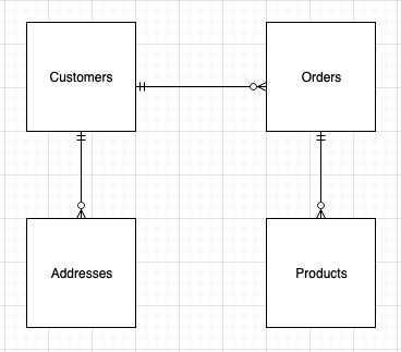
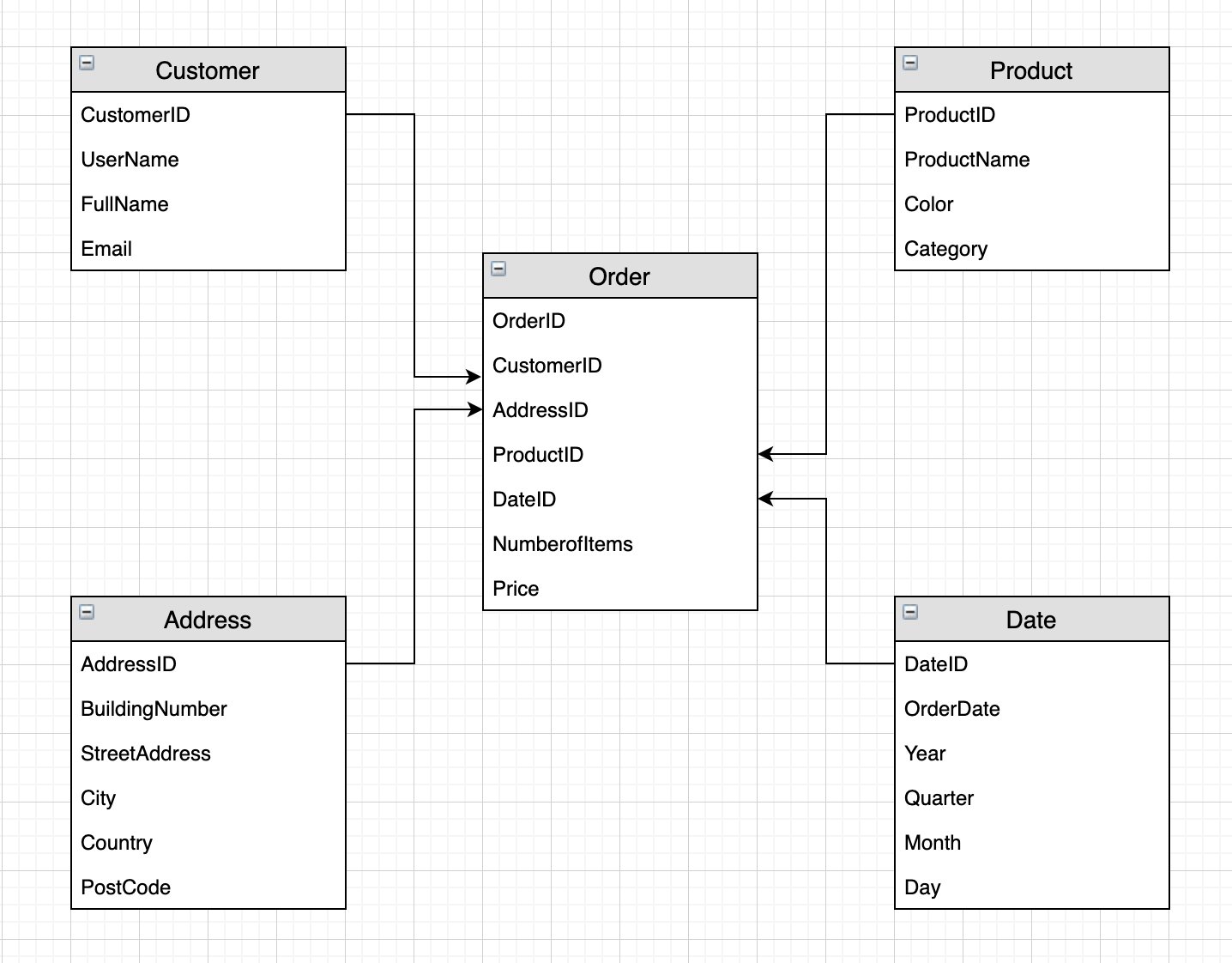
We use an example of a successful ecommerce store allowing registered users to order products from their website. A simple ERD (entity-relation diagram) for this application will have four distinct entities: customers, addresses, orders, and products. For customers, we have information such as their unique user name and email address; for the address entity, we have one or more customer addresses. Orders contain information regarding the order placed, and the products entity provides information about the products placed in an order. As we can see from the following diagram, a customer can place one or more orders, and an order must contain one or more products.

We could store each entity in a separate table in DynamoDB. However, there is no way to retrieve customer details alongside all the orders placed by the customer without making multiple requests to the customer and order tables. This is inefficient from both a cost and performance perspective. A key goal for any efficient application is to retrieve all the required information in a single query request. This ensures fast, consistent performance. So how can we remodel our data to avoid making multiple requests? One option is to use single-table design. Taking advantage of the schema-less nature of DynamoDB, we can store different types of records in a single table in order to handle different access patterns in a single request. We can go further still and store different types of values in the same attribute and use it as a global secondary index (GSI). This is called index overloading.

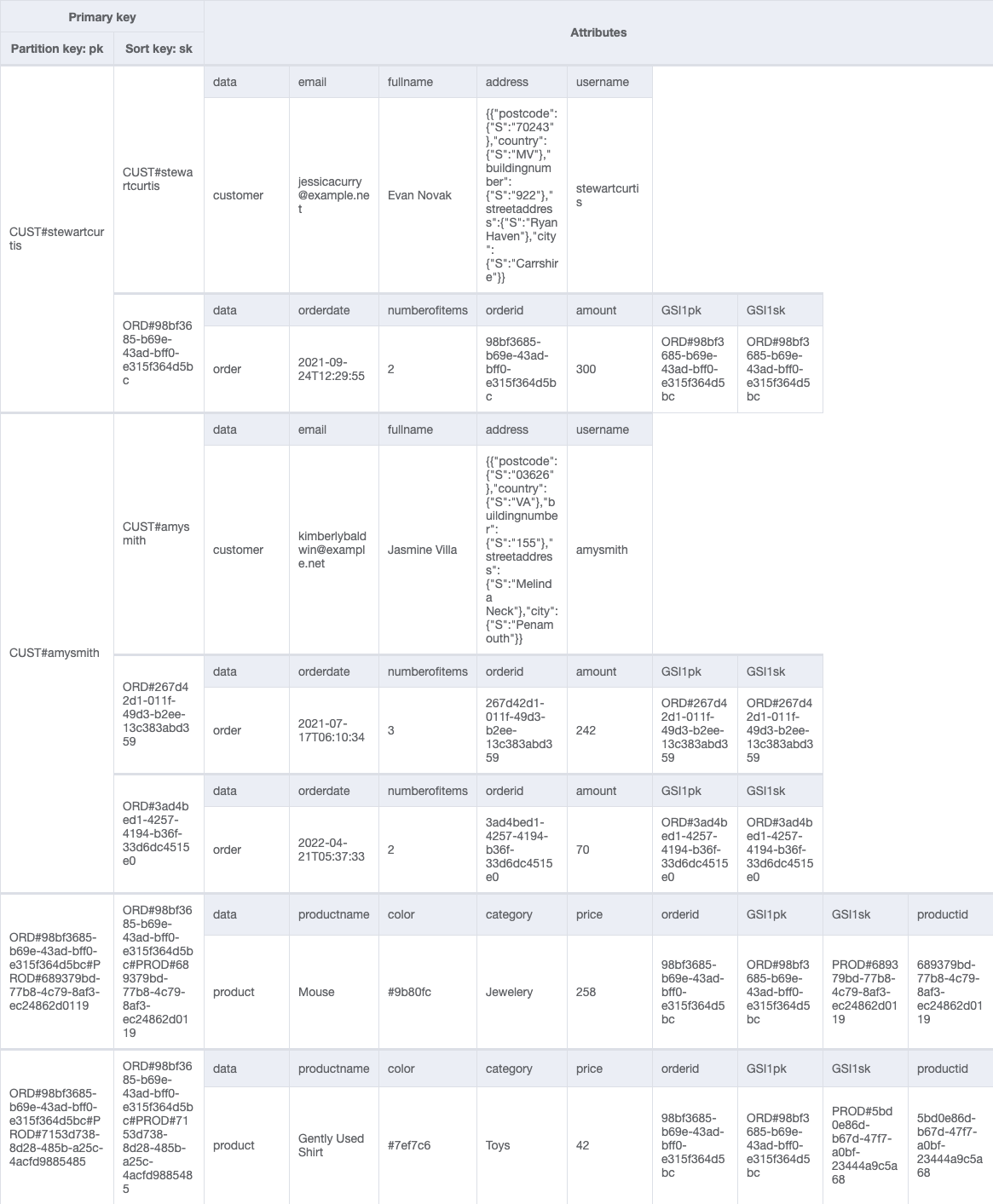
A typical access pattern we may want to handle in our single table design is to get customer details and all orders placed by the customer.

To accommodate this access pattern, our single-table design looks like the following example.

By restricting the number of addresses associated with a customer, we can store address details as a complex attribute (rather than a separate item) without exceeding the 400 KB item size limit of DynamoDB.

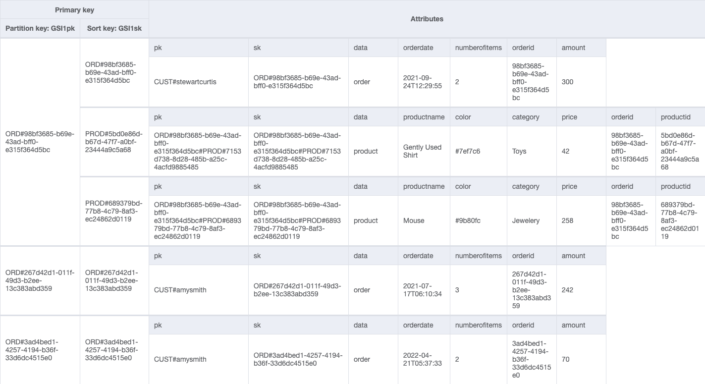
We can add a global secondary index (GSIpk and GSIsk) to capture another access pattern: get order details and all product items placed in an order. We use the following table.

We have used generic attribute names, PK and SK, for our partition key and sort key columns. This is because they hold data from different entities. Furthermore, the values in these columns are prefixed by generic terms such as CUST# and ORD# to help us identify the type of data we have and ensure that the value in PK is unique across all records in the table.

A well-designed single table will not only reduce the number of requests for an access pattern, but will service many different access patterns. The challenge comes when we need to ask more complex questions of our data, for example, what was the year-on-year quarterly sales growth by product broken down by country?

The case for a data warehouse

A data warehouse is ideally suited to answer OLAP queries. Built on highly curated structured data, it provides the flexibility and speed to run aggregations across an entire dataset to derive insights.

To house our data, we need to define a data model. An optimal design choice is to use a dimensional model. A dimension model consists of fact tables and dimension tables. Fact tables store the numeric information about business measures and foreign keys to the dimension tables. Dimension tables store descriptive information about the business facts to help understand and analyze the data better. From a business perspective, a dimension model with its use of facts and dimensions can present complex business processes in a simple-to-understand manner.

Building a dimensional model

A dimensional model optimizes read performance through efficient joins and filters. Amazon Redshift automatically chooses the best distribution style and sort key based on workload patterns. We build a dimensional model from the single DynamoDB table based on the following star schema.

We have separated each item type into individual tables. We have a single fact table (Orders) containing the business measures price and numberofitems, and foreign keys to the dimension tables. By storing the price of each product in the fact table, we can track price fluctuations in the fact table without continually updating the product dimension. (In a similar vein, the DynamoDB attribute amount is a simple derived measure in our star schema: amount is the summation of product prices per orderid).

By splitting the descriptive content of our single DynamoDB table into multiple Amazon Redshift dimension tables, we can remove redundancy by only holding in each dimension the information pertinent to it. This allows us the flexibility to query the data under different contexts; for example, we may want to know the frequency of customer orders by city or product sales by date. The ability to freely join dimensions and facts when analyzing the data is one of the key benefits of dimensional modeling. It’s also good practice to have a Date dimension to allow us to perform time-based analysis by aggregating the fact by year, month, quarter, and so forth.

This dimensional model will be built in Amazon Redshift. When setting out to build a data warehouse, it’s a common pattern to have a data lake as the source of the data warehouse. The data lake in this context serves a number of important functions:

  • It acts as a central source for multiple applications, not just exclusively for data warehousing purposes. For example, the same dataset could be used to build machine learning (ML) models to identify trends and predict sales.
  • It can store data as is, be it unstructured, semi-structured, or structured. This allows you to explore and analyze the data without committing upfront to what the structure of the data should be.
  • It can be used to offload historical or less-frequently-accessed data, allowing you to manage your compute and storage costs more effectively. In our analytic use case, if we are analyzing quarterly growth rates, we may only need a couple of years’ worth of data; the rest can be unloaded into the data lake.

When querying a data lake, we need to consider user access patterns in order to reduce costs and optimize query performance. This is achieved by partitioning the data. The choice of partition keys will depend on how you query the data. For example, if you query the data by customer or country, then they are good candidates for partition keys; if you query by date, then a date hierarchy can be used to partition the data.

After the data is partitioned, we want to ensure it’s held in the right format for optimal query performance. The recommended choice is to use a columnar format such as Parquet or ORC. Such formats are compressed and store data column-wise, allowing for fast retrieval times, and are parallelizable, allowing for fast load times when moving the data into Amazon Redshift. In our use case, it makes sense to store the data in a data lake with minimal transformation and formatting to enable easy querying and exploration of the dataset. We partition the data by item type (Customer, Order, Product, and so on), and because we want to easily query each entity in order to move the data into our data warehouse, we transform the data into the Parquet format.

Solution overview

The following diagram illustrates the data flow to export data from a DynamoDB table to a data warehouse.

We present a batch ELT solution using AWS Glue for exporting data stored in DynamoDB to an Amazon Simple Storage Service (Amazon S3) data lake and then a data warehouse built in Amazon Redshift. AWS Glue is a fully managed extract, transform, and load (ETL) service that allows you to organize, cleanse, validate, and format data for storage in a data warehouse or data lake.

The solution workflow has the following steps:

  1. Move any existing files from the raw and data lake buckets into corresponding archive buckets to ensure any fresh export from DynamoDB to Amazon S3 isn’t duplicating data.
  2. Begin a new DynamoDB export to the S3 raw layer.
  3. From the raw files, create a data lake partitioned by item type.
  4. Load the data from the data lake to landing tables in Amazon Redshift.
  5. After the data is loaded, we take advantage of the distributed compute capability of Amazon Redshift to transform the data into our dimensional model and populate the data warehouse.

We orchestrate the pipeline using an AWS Step Functions workflow and schedule a daily batch run using Amazon EventBridge.

For simpler DynamoDB table structures you may consider skipping some of these steps by either loading data directly from DynamoDB to Redshift or using Redshift’s auto-copy or copy command to load data from S3.

Prerequisites

You must have an AWS account with a user who has programmatic access. For setup instructions, refer to AWS security credentials.

Use the AWS CloudFormation template cf_template_ddb-dwh-blog.yaml to launch the following resources:

  • A DynamoDB table with a GSI and point-in-time recovery enabled.
  • An Amazon Redshift cluster (we use two nodes of RA3.4xlarge).
  • Three AWS Glue database catalogs: raw, datalake, and redshift.
  • Five S3 buckets: two for the raw and data lake files; two for their respective archives, and one for the Amazon Athena query results.
  • Two AWS Identity and Access Management (IAM) roles: An AWS Glue role and a Step Functions role with the requisite permissions and access to resources.
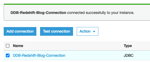
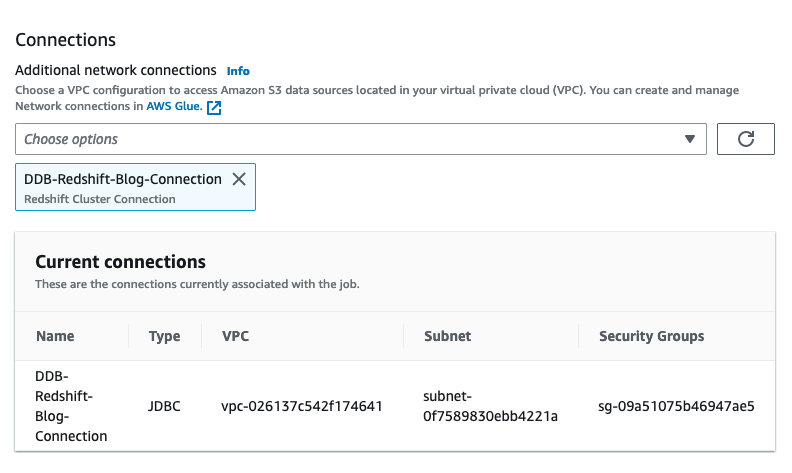
  • A JDBC connection to Amazon Redshift.
  • An AWS Lambda function to retrieve the s3-prefix-list-id for your Region. This is required to allow traffic from a VPC to access an AWS service through a gateway VPC endpoint.
  • Download the following files to perform the ELT:
    • The Python script to load sample data into our DynamoDB table: load_dynamodb.py.
    • The AWS Glue Python Spark script to archive the raw and data lake files: archive_job.py.
    • The AWS Glue Spark scripts to extract and load the data from DynamoDB to Amazon Redshift: GlueSparkJobs.zip.
    • The DDL and DML SQL scripts to create the tables and load the data into the data warehouse in Amazon Redshift: SQL Scripts.zip.

Launch the CloudFormation template

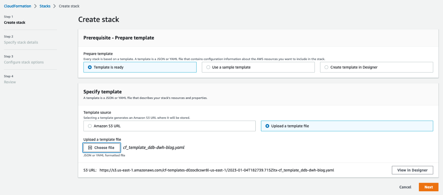
AWS CloudFormation allows you to model, provision, and scale your AWS resources by treating infrastructure as code. We use the downloaded CloudFormation template to create a stack (with new resources).

  1. On the AWS CloudFormation console, create a new stack and select Template is ready.
  2. Upload the stack and choose Next.

  1. Enter a name for your stack.
  2. For MasterUserPassword, enter a password.
  3. Optionally, replace the default names for the Amazon Redshift database, DynamoDB table, and MasterUsername (in case these names are already in use).
  4. Reviewed the details and acknowledge that AWS CloudFormation may create IAM resources on your behalf.
  5. Choose Create stack.

Load sample data into a DynamoDB table

To load your sample data into DynamoDB, complete the following steps:

  1. Create an AWS Cloud9 environment with default settings.
  2. Upload the load DynamoDB Python script. From the AWS Cloud9 terminal, use the pip install command to install the following packages:
    1. boto3
    2. faker
    3. faker_commerce
    4. numpy
  3. In the Python script, replace all placeholders (capital letters) with the appropriate values and run the following command in the terminal:
python load_dynamodb.py

This command loads the sample data into our single DynamoDB table.

Extract data from DynamoDB

To extract the data from DynamoDB to our S3 data lake, we use the new AWS Glue DynamoDB export connector. Unlike the old connector, the new version uses a snapshot of the DynamoDB table and doesn’t consume read capacity units of your source DynamoDB table. For large DynamoDB tables exceeding 100 GB, the read performance of the new AWS Glue DynamoDB export connector is not only consistent but also significantly faster than the previous version.

To use this new export connector, you need to enable point-in-time recovery (PITR) for the source DynamoDB table in advance. This will take continuous backups of the source table (so be mindful of cost) and ensures that each time the connector invokes an export, the data is fresh. The time it takes to complete an export depends on the size of your table and how uniformly the data is distributed therein. This can range from a few minutes for small tables (up to 10 GiB) to a few hours for larger tables (up to a few terabytes). This is not a concern for our use case because data lakes and data warehouses are typically used to aggregate data at scale and generate daily, weekly, or monthly reports. It’s also worth noting that each export is a full refresh of the data, so in order to build a scalable automated data pipeline, we need to archive the existing files before beginning a fresh export from DynamoDB.

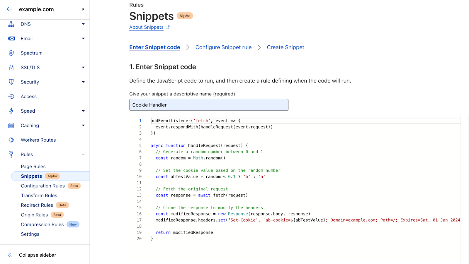
Complete the following steps:

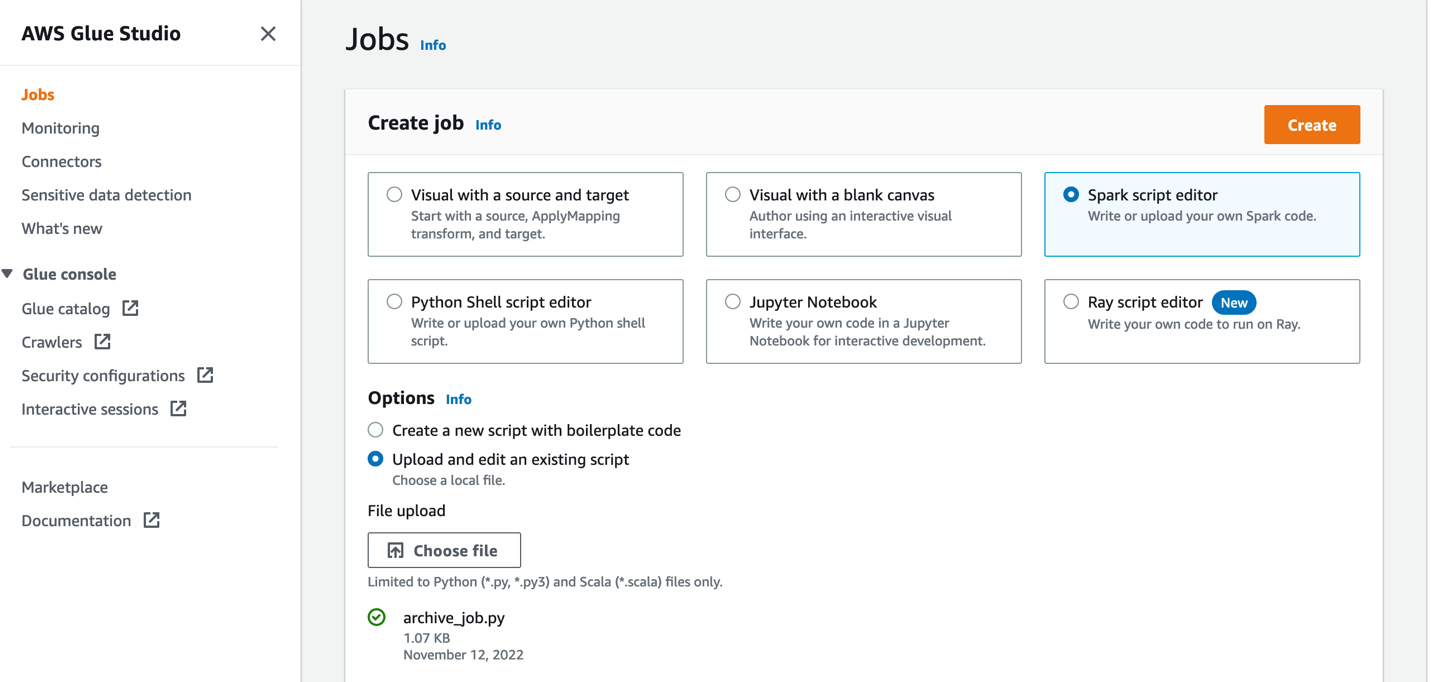
  1. Create an AWS Glue job using the Spark script editor.
  2. Upload the archive_job.py file from GlueSparkJobs.zip.

This job archives the data files into timestamped folders. We run the job concurrently to archive the raw files and the data lake files.

  1. In Job details section, give the job a name and choose the AWS Glue IAM role created by our CloudFormation template.
  2. Keep all defaults the same and ensure maximum concurrency is set to 2 (under Advanced properties).

Archiving the files provides a backup option in the event of disaster recovery. As such, we can assume that the files will not be accessed frequently and can be kept in Standard_IA storage class so as to save up to 40% on costs while providing rapid access to the files when needed.

This job typically runs before each export of data from DynamoDB. After the datasets have been archived, we’re ready to (re)-export the data from our DynamoDB table.

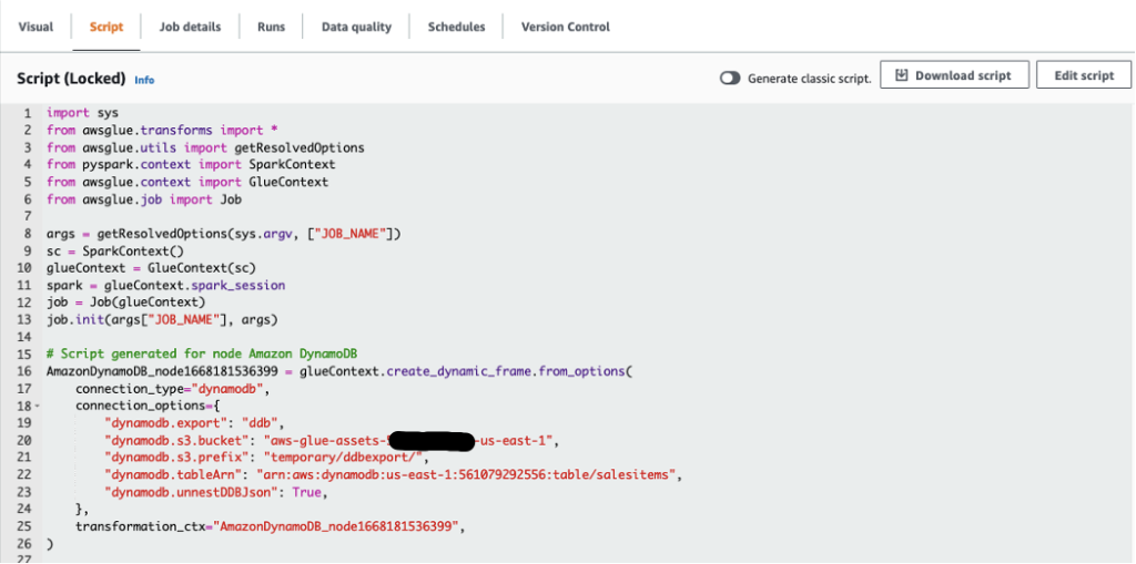
We can use AWS Glue Studio to visually create the jobs needed to extract the data from DynamoDB and load into our Amazon Redshift data warehouse. We demonstrate how to do this by creating an AWS Glue job (called ddb_export_raw_job) using AWS Glue Studio.

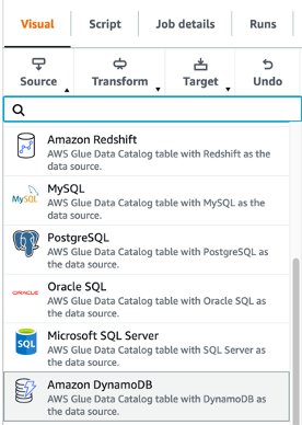
  1. In AWS Glue Studio, create a job and select Visual with a blank canvas.
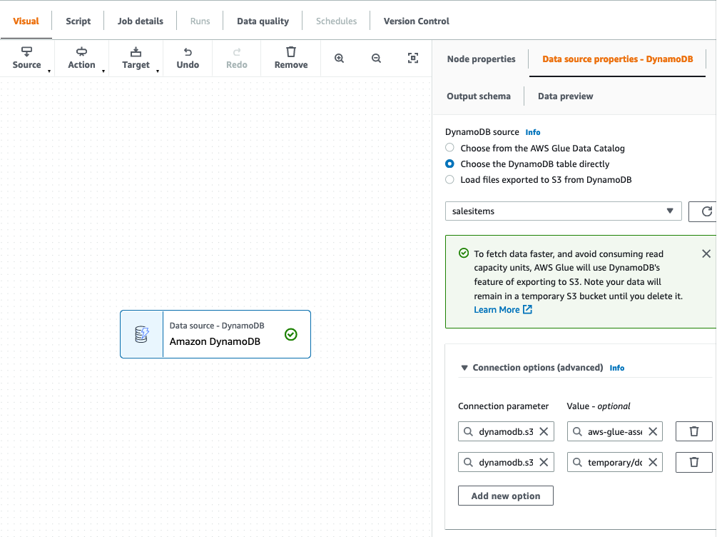
  2. Choose Amazon DynamoDB as the data source.

  1. Choose our DynamoDB table to export from.
  2. Leave all other options as is and finish setting up the source connection.

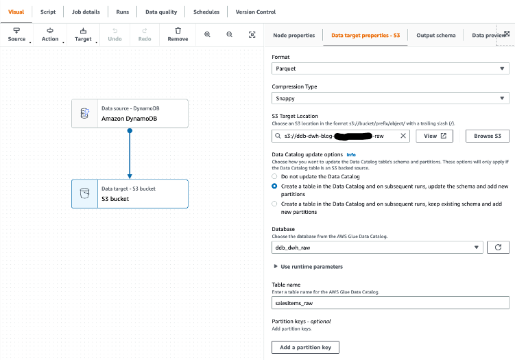
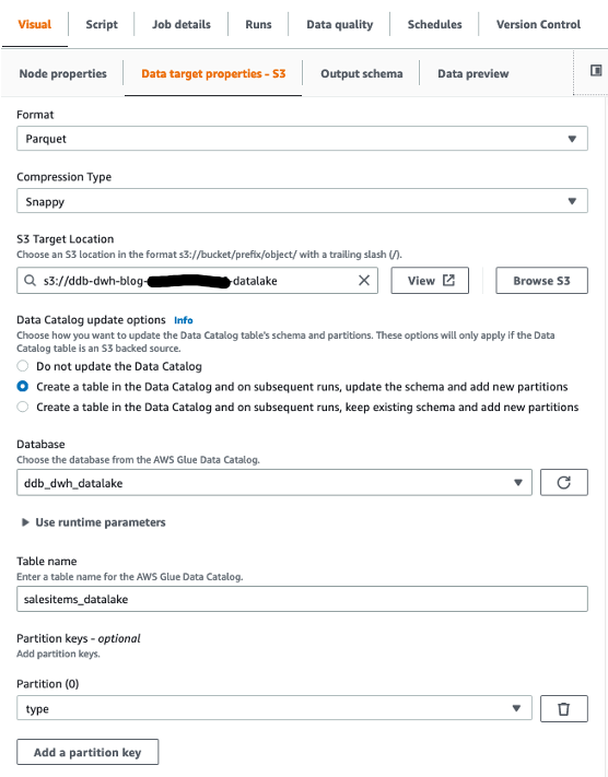
We then choose Amazon S3 as our target. In the target properties, we can transform the output to a suitable format, apply compression, and specify the S3 location to store our raw data.

  1. Set the following options:
    1. For Format, choose Parquet.
    2. For Compression type, choose Snappy.
    3. For S3 Target Location, enter the path for RawBucket (located on the Outputs tab of the CloudFormation stack).
    4. For Database, choose the value for GlueRawDatabase (from the CloudFormation stack output).
    5. For Table name, enter an appropriate name.

  1. Because our target data warehouse requires data to be in a flat structure, verify that the configuration option dynamodb.unnestDDBJson is set to True on the Script tab.

  1. On the Job details tab, choose the AWS Glue IAM role generated by the CloudFormation template.
  2. Save and run the job.

Depending on the data volumes being exported, this job may take a few minutes to complete.

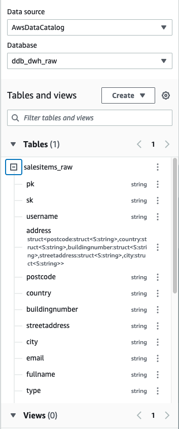
Because we’ll be adding the table to our AWS Glue Data Catalog, we can explore the output using Athena after the job is complete. Athena is a serverless interactive query service that makes it simple to analyze data directly in Amazon S3 using standard SQL.

  1. In the Athena query editor, choose the raw database.

We can see that the attributes of the Address structure have been unnested and added as additional columns to the table.

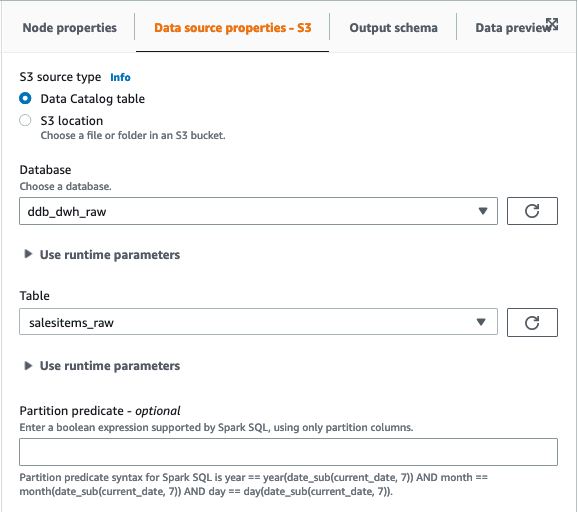
  1. After we export the data into the raw bucket, create another job (called raw_to_datalake_job) using AWS Glue Studio (select Visual with a blank canvas) to load the data lake partitioned by item type (customer, order, and product).
  2. Set the source as the AWS Glue Data Catalog raw database and table.

  1. In the ApplyMapping transformation, drop the Address struct because we have already unnested these attributes into our flattened raw table.

  1. Set the target as our S3 data lake.

  1. Choose the AWS Glue IAM role in the job details, then save and run the job.

Now that we have our data lake, we’re ready to build our data warehouse.

Build the dimensional model in Amazon Redshift

The CloudFormation template launches a two-node RA3.4xlarge Amazon Redshift cluster. To build the dimensional model, complete the following steps:

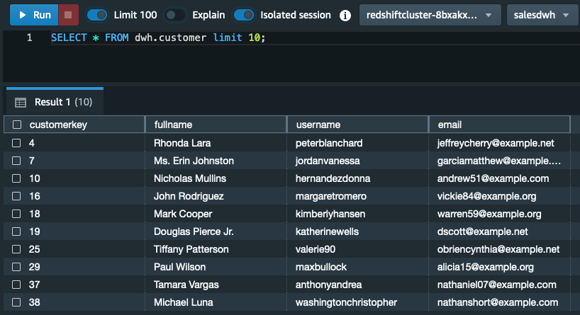
  1. In Amazon Redshift Query Editor V2, connect to your database (default: salesdwh) within the cluster using the database user name and password authentication (MasterUserName and MasterUserPassword from the CloudFormation template).
  2. You may be asked to configure your account if this is your first time using Query Editor V2.
  3. Download the SQL scripts SQL Scripts.zip to create the following schemas and tables (run the scripts in numbered sequence).

In the landing schema:

  • address
  • customer
  • order
  • product

In the staging schema:

  • staging.address
  • staging.address_maxkey
  • staging.addresskey
  • staging.customer
  • staging.customer_maxkey
  • staging.customerkey
  • staging.date
  • staging.date_maxkey
  • staging.datekey
  • staging.order
  • staging.order_maxkey
  • staging.orderkey
  • staging.product
  • staging.product_maxkey
  • staging.productkey

In the dwh schema:

  • dwh.address
  • dwh.customer
  • dwh.order
  • dwh.product

We load the data from our data lake to the landing schema as is.

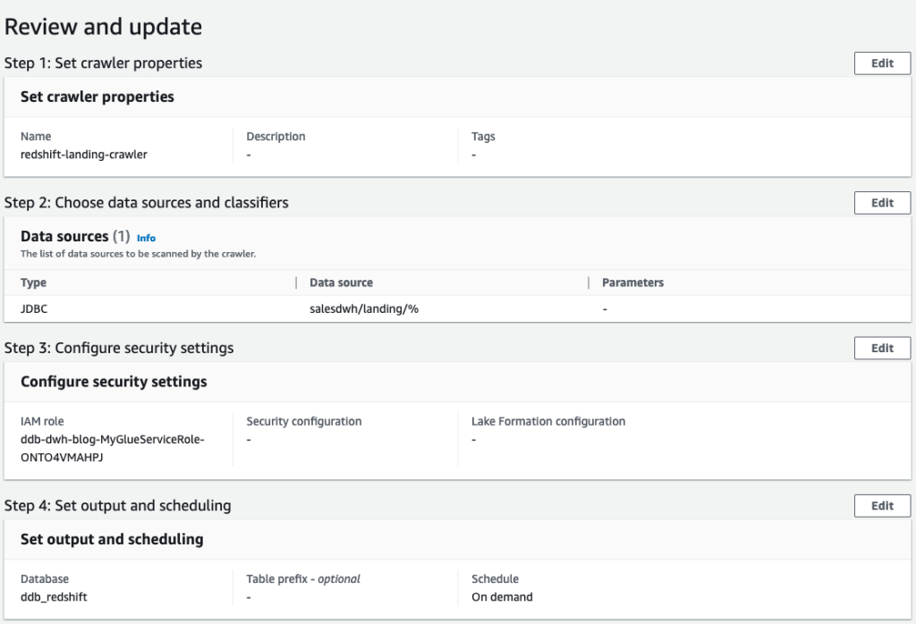
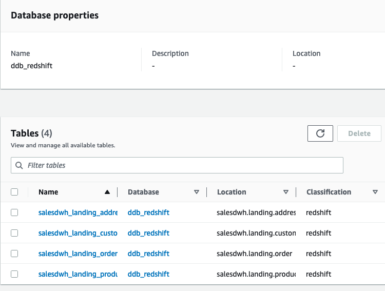
  1. Use the JDBC connector to Amazon Redshift to build an AWS Glue crawler to add the landing schema to our Data Catalog under the ddb_redshift database.

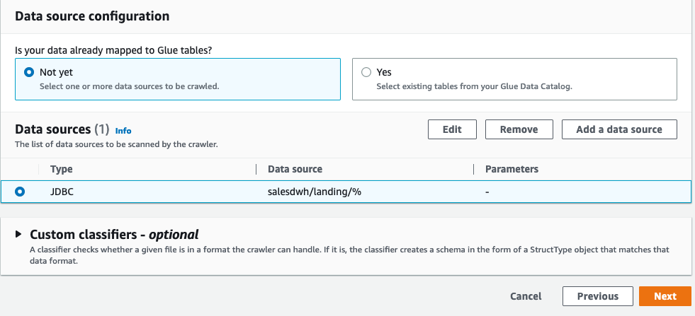
  1. Create an AWS Glue crawler with the JDBC data source.

  1. Select the JDBC connection you created and choose Next.

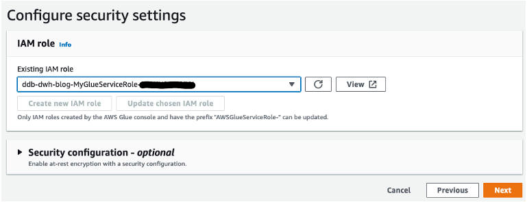
  1. Choose the IAM role created by the CloudFormation template and choose Next.

  1. Review your settings before creating the crawler.

The crawler adds the four landing tables in our AWS Glue database ddb_redshift.

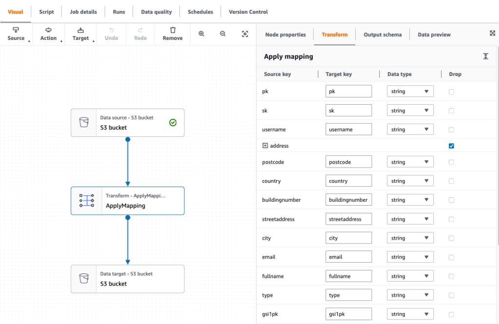
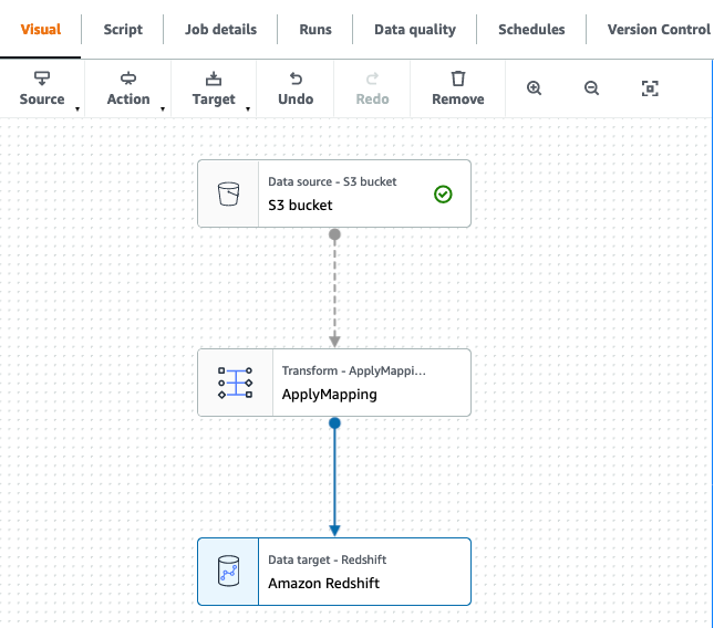
  1. In AWS Glue Studio, create four AWS Glue jobs to load the landing tables (these scripts are available to download, and you can use the Spark script editor to upload these scripts individually to create the jobs):
    1. land_order_job
    2. land_product_job
    3. land_customer_job
    4. land_address_job

Each job has the structure as shown in the following screenshot.

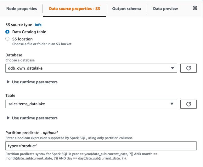
  1. Filter the S3 source on the partition column type:
    1. For product, filter on type=‘product’.
    2. For order, filter on type=‘order’.
    3. For customer and address, filter on type=‘customer’.

  1. Set the target for the data flow as the corresponding table in the landing schema in Amazon Redshift.
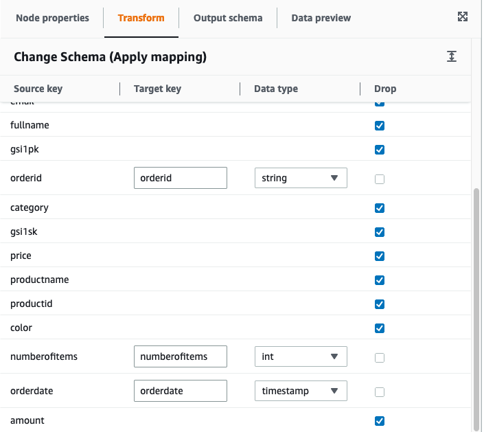
  2. Use the built-in ApplyMapping transformation in our data pipeline to drop columns and, where necessary, convert the data types to match the target columns.

For more information about built-in transforms available in AWS Glue, refer to AWS Glue PySpark transforms reference.

The mappings for our four jobs are as follows:

  • land_order_job:
    mappings=[
    ("pk", "string", "pk", "string"),
    ("orderid", "string", "orderid", "string"),
    ("numberofitems", "string", "numberofitems", "int"),
    ("orderdate", "string", "orderdate", "timestamp"),
    ]

  • land_product_job:
    mappings=[
    ("orderid", "string", "orderid", "string"),
    ("category", "string", "category", "string"),
    ("price", "string", "price", "decimal"),
    ("productname", "string", "productname", "string"),
    ("productid", "string", "productid", "string"),
    ("color", "string", "color", "string"),
    ]

  • land_address_job:
    mappings=[
    ("username", "string", "username", "string"),
    ("email", "string", "email", "string"),
    ("fullname", "string", "fullname", "string"),
    ]

  • land_customer_job:
    mappings=[
    ("username", "string", "username", "string"),
    ("email", "string", "email", "string"),
    ("fullname", "string", "fullname", "string"),
    ]

  1. Choose the AWS Glue IAM role, and under Advanced properties, verify the JDBC connector to Amazon Redshift as a connection.
  2. Save and run each job to load the landing tables in Amazon Redshift.

Populate the data warehouse

From the landing schema, we move the data to the staging layer and apply the necessary transformations. Our dimensional model has a single fact table, the orders table, which is the largest table and as such needs a distribution key. The choice of key depends on how the data is queried and the size of the dimension tables being joined to. If you’re unsure of your query patterns, you can leave the distribution keys and sort keys for your tables unspecified. Amazon Redshift automatically assigns the correct distribution and sort keys based on your queries. This has the advantage that if and when query patterns change over time, Amazon Redshift can automatically update the keys to reflect the change in usage.

In the staging schema, we keep track of existing records based on their business key (the unique identifier for the record). We create key tables to generate a numeric identity column for each table based on the business key. These key tables allow us to implement an incremental transformation of the data into our dimensional model.

CREATE TABLE IF NOT EXISTS staging.productkey ( 
    productkey integer identity(1,1), 
    productid character varying(16383), 
    CONSTRAINT products_pkey PRIMARY KEY(productkey));   

When loading the data, we need to keep track of the latest surrogate key value to ensure that new records are assigned the correct increment. We do this using maxkey tables (pre-populated with zero):

CREATE TABLE IF NOT EXISTS staging.product_maxkey ( 
    productmaxkey integer);

INSERT INTO staging.product_maxkey
select 0;    

We use staging tables to store our incremental load, the structure of which will mirror our final target model in the dwh schema:

---staging tables to load data from data lake 
   
CREATE TABLE IF NOT EXISTS staging.product ( 
    productkey integer,
    productname character varying(200), 
    color character varying(50), 
    category character varying(100),
    PRIMARY KEY (productkey));
---dwh tables to load data from staging schema
     
CREATE TABLE IF NOT EXISTS dwh.product ( 
    productkey integer,
    productname character varying(200), 
    color character varying(50), 
    category character varying(100),
    PRIMARY KEY (productkey)); 

Incremental processing in the data warehouse

We load the target data warehouse using stored procedures to perform upserts (deletes and inserts performed in a single transaction):

CREATE OR REPLACE PROCEDURE staging.load_order() LANGUAGE plpgsql AS $$
DECLARE
BEGIN

TRUNCATE TABLE staging.order;

--insert new records to get new ids
insert into staging.orderkey
(
orderid
)
select
c.orderid
from landing.order c
LEFT JOIN staging.orderkey i
ON c.orderid=i.orderid
where i.orderid IS NULL;

--update the max key
update staging.order_maxkey
set ordermaxkey = (select max(orderkey) from staging.orderkey);


insert into staging.order
(
orderkey,
customerkey,
productkey,
addresskey,
datekey,
numberofitems,
price
)
select
xid.orderkey,
cid.customerkey,
pid.productkey,
aid.addresskey,
d.datekey,
o.numberofitems,
p.price
from
landing.order o
join staging.orderkey xid on o.orderid=xid.orderid
join landing.customer c on substring(o.pk,6,length(o.pk))=c.username   ---order table needs username
join staging.customerkey cid on cid.username=c.username
join landing.address a on a.username=c.username
join staging.addresskey aid on aid.pk=a.buildingnumber::varchar+'||'+a.postcode  ---maybe change pk to addressid
join staging.datekey d on d.orderdate=o.orderdate
join landing.product p on p.orderid=o.orderid
join staging.productkey pid on pid.productid=p.productid;

COMMIT;

END;
$$ 
CREATE OR REPLACE PROCEDURE dwh.load_order() LANGUAGE plpgsql AS $$
DECLARE
BEGIN

---delete old records 
delete from dwh.order
using staging.order as stage
where dwh.order.orderkey=stage.orderkey;

--insert new and modified
insert into dwh.order
(
orderkey,
customerkey,  
productkey,
addresskey,
price,
datekey  
)
select
orderkey,
customerkey,  
productkey,
addresskey,
price,
datekey
from staging.order;

COMMIT;
END;
$$

Use Step Functions to orchestrate the data pipeline

So far, we have stepped through each component in our workflow. We now need to stitch them together to build an automated, idempotent data pipeline. A good orchestration tool must manage failures, retries, parallelization, service integrations, and observability, so developers can focus solely on the business logic. Ideally, the workflow we build is also serverless so there is no operational overhead. Step Functions is an ideal choice to automate our data pipeline. It allows us to integrate the ELT components we have built on AWS Glue and Amazon Redshift and conduct some steps in parallel to optimize performance.

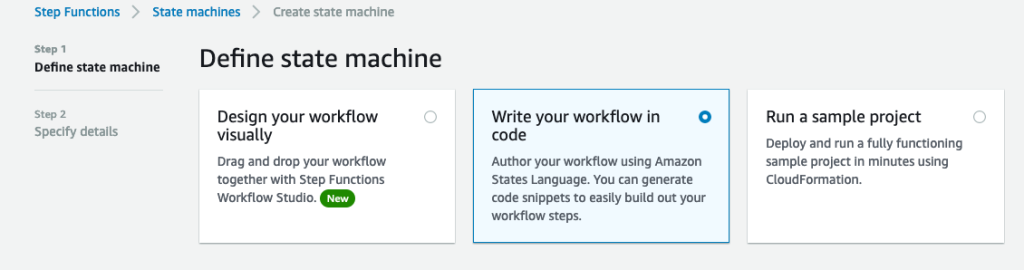
  1. On the Step Functions console, create a new state machine.
  2. Select Write your workflow in code.

  1. Enter the stepfunction_workflow.json code into the definition, replacing all placeholders with the appropriate values:
    1. [REDSHIFT-CLUSTER-IDENTIFIER] – Use the value for ClusterName (from the Outputs tab in the CloudFormation stack).
    2. [REDSHIFT-DATABASE] – Use the value for salesdwh (unless changed, this is the default database in the CloudFormation template).

We use the Step Functions IAM role from the CloudFormation template.

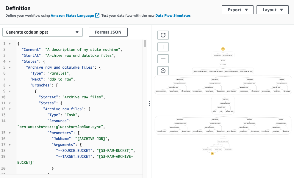
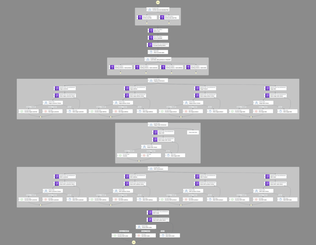
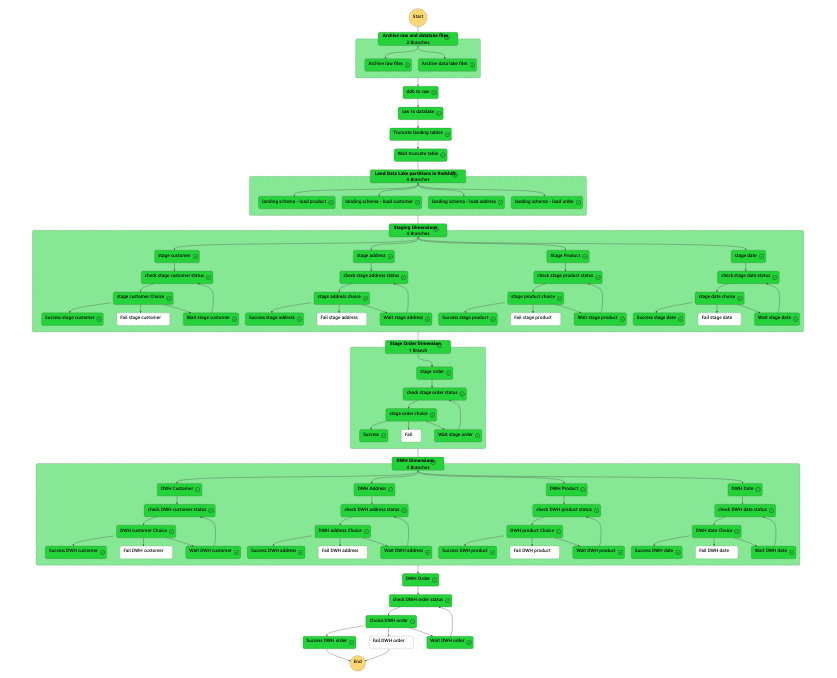
This JSON code generates the following pipeline.

Starting from the top, the workflow contains the following steps:

  1. We archive any existing raw and data lake files.
  2. We add two AWS Glue StartJobRun tasks that run sequentially: first to export the data from DynamoDB to our raw bucket, then from the raw bucket to our data lake.
  3. After that, we parallelize the landing of data from Amazon S3 to Amazon Redshift.
  4. We transform and load the data into our data warehouse using the Amazon Redshift Data API. Because this is asynchronous, we need to check the status of the runs before moving down the pipeline.
  5. After we move the data load from landing to staging, we truncate the landing tables.
  6. We load the dimensions of our target data warehouse (dwh) first, and finally we load our single fact table with its foreign key dependency on the preceding dimension tables.

The following figure illustrates a successful run.

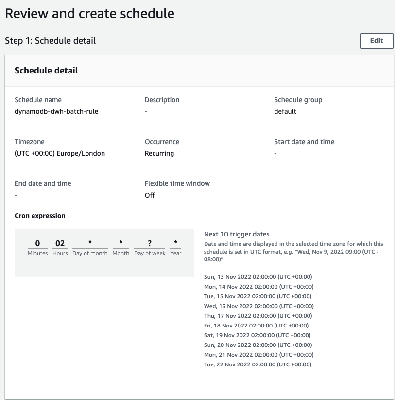
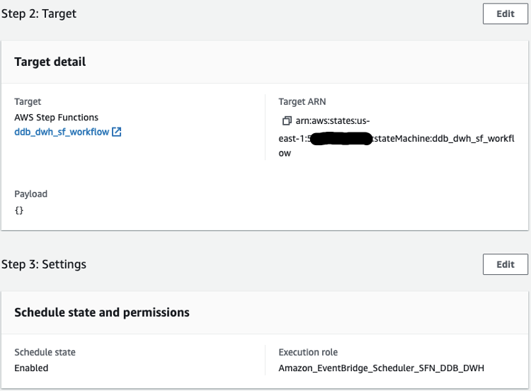
After we set up the workflow, we can use EventBridge to schedule a daily midnight run, where the target is a Step Functions StartExecution API calling our state machine. Under the workflow permissions, choose Create a new role for this schedule and optionally rename it.

Query the data warehouse

We can verify the data has been successfully loaded into Amazon Redshift with a query.

After we have the data loaded into Amazon Redshift, we’re ready to answer the query asked at the start of this post: what is the year-on-year quarterly sales growth by product and country? The query looks like the following code (depending on your dataset, you may need to select alternative years and quarters):

with sales2021q2
as
(
  select d.year, d.quarter,a.country,p.category,sum(o.price) as revenue2021q2
  from dwh.order o
  join dwh.date d on o.datekey=d.datekey
  join dwh.product p on o.productkey=p.productkey
  join dwh.address a on a.addresskey=o.addresskey
  where d.year=2021 and d.quarter=2
  group by d.year, d.quarter,a.country,p.category
  ),
sales2022q2
as
(
  select d.year, d.quarter,a.country,p.category,sum(o.price) as revenue2022q2
  from dwh.order o
  join dwh.date d on o.datekey=d.datekey
  join dwh.product p on o.productkey=p.productkey
  join dwh.address a on a.addresskey=o.addresskey
  where d.year=2022 and d.quarter=2
  group by d.year, d.quarter,a.country,p.category
  )

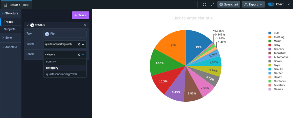
select a.country,a.category, ((revenue2022q2 - revenue2021q2)/revenue2021q2)*100 as quarteronquartergrowth
from sales2022q2 a
join sales2021q2 b on a.country=b.country and a.category=b.category
order by a.country,a.category

We can visualize the results in Amazon Redshift Query Editor V2 by toggling the chart option and setting Type as Pie, Values as quarteronquartergrowth, and Labels as category.

Cost considerations

We give a brief outline of the indicative costs associated with the key services covered in our solution based on us-east-1 Region pricing using the AWS Pricing Calculator:

  • DynamoDB – With on-demand settings for 1.5 million items (average size of 355 bytes) and associated write and read capacity plus PITR storage, the cost of DynamoDB is approximately $2 per month.
  • AWS Glue DynamoDB export connector – This connector utilizes the DynamoDB export to Amazon S3 feature. This has no hourly cost—you only pay for the gigabytes of data exported to Amazon S3 ($0.11 per GiB).
  • Amazon S3 – You pay for storing objects in your S3 buckets. The rate you’re charged depends on your objects’ size, how long you stored the objects during the month, and the storage class. In our solution, we used S3 Standard for our data lake and S3 Standard – Infrequent Access for archive. Standard-IA storage is $0.0125 per GB/month; Standard storage is $0.023 per GB/month.
  • AWS Glue Jobs – With AWS Glue, you only pay for the time your ETL job takes to run. There are no resources to manage, no upfront costs, and you are not charged for startup or shutdown time. AWS charges you an hourly rate based on the number of Data Processing Units (DPUs) used to run your ETL job. A single DPU provides 4 vCPU and 16 GB of memory. Every one of our nine Spark jobs uses 10 DPUs and has an average runtime of 3 minutes. This gives an approximate cost of $0.29 per job.
  • Amazon Redshift – We provisioned two RA3.4xlarge nodes for our Amazon Redshift cluster. If run on-demand, each node costs $3.26 per hour. If utilized 24/7, our monthly cost would be approximately $4,759.60. You should evaluate your workload to determine what cost savings can be achieved by using Amazon Redshift Serverless or using Amazon Redshift provisioned reserved instances.
  • Step Functions – You are charged based on the number of state transitions required to run your application. Step Functions counts a state transition as each time a step of your workflow is run. You’re charged for the total number of state transitions across all your state machines, including retries. The Step Functions free tier includes 4,000 free state transitions per month. Thereafter, it’s $0.025 per 1,000 state transitions.

Clean up

Remember to delete any resources created through the CloudFormation stack. You first need to manually empty and delete the S3 buckets. Then you can delete the CloudFormation stack using the AWS CloudFormation console or AWS Command Line Interface (AWS CLI). For instructions, refer to Clean up your “hello, world!” application and related resources.

Summary

In this post, we demonstrated how you can export data from DynamoDB to Amazon S3 and Amazon Redshift to perform advanced analytics. We built an automated data pipeline that you can use to perform a batch ELT process that can be scheduled to run daily, weekly, or monthly and can scale to handle very large workloads.

Please leave your feedback or comments in the comments section.


About the Author

Altaf Hussain is an Analytics Specialist Solutions Architect at AWS. He helps customers around the globe design and optimize their big data and data warehousing solutions.


Appendix

To extract the data from DynamoDB and load it into our Amazon Redshift database, we can use the Spark script editor and upload the files from GlueSparkJobs.zip to create each individual job necessary to perform the extract and load. If you choose to do this, remember to update, where appropriate, the account ID and Region placeholders in the scripts. Also, on the Job details tab under Advanced properties, add the Amazon Redshift connection.

Red Hat cutting back RHEL source availability

Post Syndicated from original https://lwn.net/Articles/935592/

Red Hat has announced
that public source releases will be restricted to CentOS Stream going
forward:

As the CentOS Stream community grows and the enterprise software
world tackles new dynamics, we want to sharpen our focus on CentOS
Stream as the backbone of enterprise Linux innovation. We are
continuing our investment in and increasing our commitment to
CentOS Stream. CentOS Stream will now be the sole repository for
public RHEL-related source code releases
. For Red Hat customers
and partners, source code will remain available via the Red Hat
Customer Portal.

(Emphasis in original; thanks to Janne Blomqvist).

How to send messages to multiple recipients with Amazon Simple Email Service (SES)

Post Syndicated from Joydeep Dutta original https://aws.amazon.com/blogs/messaging-and-targeting/how-to-send-messages-to-multiple-recipients-with-amazon-simple-email-service-ses/

Introduction

Customers frequently ask what is the best way to send messages to multiple recipients using Amazon Simple Email Service (SES) with the best deliverability and without exceeding the maximum recipient’s per message limit. In this blog, we will show you how to determine the best approach for sending a message to multiple recipients based on different use-cases. We will also discuss why in most situations sending messages to a single recipient at a time is the best approach.

Difference between message Header addresses and Envelope addresses

Before we dive into the use cases, let’s discuss how message addressing works in SES. When a client makes a request, SES constructs an email message compliant with the RFC 5322 Internet Message Format specification . An email comprises of a header, a body, and an RFC 5321 envelope, as described in the Email format in Amazon SES document.

The email addresses in the RFC 5322 To, Cc and Bcc headers are for display. These headers enable your email client interface to display to whom the message was addressed. These addresses do not control which recipients receive the messages; the envelope addresses do. The sending mail client provides the envelope recipient addresses to a mail server using the RFC 5321 RCPT TO commands. RCPT is an abbreviation for recipient.

An apt analogy (see diagram below) is how a physical letter within an envelope can address a person whose address is not the envelope. The address on the envelope is what the mail carrier to deliver the envelope. The postal worker should not need to open the envelope to know which address to deliver the mail.

Analogy to show physical mail compares to electronic mail

As an example, a school district may send letters informing residents of enrollment details for their children, but they do not know all of the names of the people who live at each address. The envelope may only list the address, and the letter may just be addressed “To Resident” if the school district doesn’t have a name to address the letter. The message is delivered to the resident’s address regardless of the accuracy of the information on the letter.

To simplify, let’s summarize the differences between To & Cc header and envelope addresses:

Header To & Cc Addresses Envelope Addresses (RCPT)
Used by email clients to display the list of recipients Used by mail servers to deliver the email message
Not used for mail delivery Used for mail delivery
Displayed to recipients Not displayed to recipients

The Bcc address is different than the To and Cc headers because it is used to send a copy of the message to an additional set of recipients that are “blind” to the other recipients. Bcc addresses are only defined by envelope addresses, not as a header address. Mail servers will commonly remove a Bcc header when handling a message, but delivery to the envelope recipient address still occurs.

When to use multiple recipients in a Destination

SES supports sending messages to multiple recipients in a single SendEmail operation. The Destination argument of the SendEmail operation represents the destination of the message. A Destination consists of To, Cc, and Bcc fields which represent both the header addresses and the envelope addresses.

When multiple recipients are defined in the Destination argument to the SendEmail operation, the defining characteristic is that every recipient receives the exact same message with the same message-id. A message-id is used for event handling (bounces, complaints, etc) among other purposes. A message-id pertains to exactly one version of a particular message.

Did you know: The use cases for recipients having a message with the same message-id are limited to situations in which the recipients are expected to interact with the message as a group. For example, recipients may reply-all to the email and have a resulting email conversation. The original message-id is used by email client applications to display a “conversation” view using the References and In-Reply-To headers. This behavior may be a good fit if the use case is a mailing list or internal announcement to employees within a company.

The recipient limit in the Destination argument is 50 because that is a reasonable break-point when the “conversational” use case runs the risk of the “reply all storm“ described in the next section. Consider using a robust mailing list solution or hosted service with capabilities similar to GNU Mailman to facilitate large group email conversations.

Why bulk mail recipients should not see other recipients

For bulk sending purposes, and most transactional sending, the recipients don’t need to know that other recipients also received the message:

  • The recipients likely gain no value from seeing the other recipient addresses, as they may be arbitrarily segmented into batches of 50 or less, and most email client interfaces have trouble displaying more than 50 addresses.
  • There is a risk of a “reply-all storm“, which is when a recipient replies to all of the To and Cc addresses from the original message, and then those people reply back asking everyone to stop replying. This scenario is fun to talk about around the water cooler, but should be avoided.
  • If recipients are defined as Bcc recipients in the Destinations argument of the SendEmail operation, it would not contain a To address, and that can look suspicious when read by the recipients.

Note: There is no authentication mechanism protecting the To or Cc headers from spoofing, so be careful about assuming any trust placed into the values of those headers. This means that it is possible for an attacker to spoof the To or Cc headers in an email message. Therefor the only meaningful address to include in the To header is the recipient’s own address, which they know isn’t spoofed because of the fact that they are reading the message.

For bulk mail it is best practice to have each recipient see only their own name and email address in the To header of the messages they receive. This makes the messages look more personable and can improve deliverability and recipient engagement.

This approach can be achieved by sending the message to each recipient individually via the SendEmail operation. You would use a single address in the “ToAddressses” field of the “Destination” argument.

Use the ToAddress field to individual message in the SendEmail API

How email event notifications are associated with recipients

If you need email event notifications to be associated to each recipient, then you will need each recipient to receive a message with a unique message-id; one recipient per Destination.

The following event types will be associated with every recipient in the Destination:

  • asynchronous bounces
  • complaints
  • opens
  • clicks

Learn more about Amazon SES events in the documentation: how email sending works in Amazon SES

For example, if one of the recipients triggers a open engagement event, and if that recipient was in a group of 50 recipients within the Destination argument to the SendEmail operation, then all 50 of those recipients will be registered as having opened the message.

Other considerations:

  • If the recipients are defined by ToAddresses and CcAddresses they will all appear in the message headers, but the To and Cc headers will be truncated in the event notifications if the headers are over 10 KB. Multi-recipient Destinations may cause you to lose observability needed to troubleshoot deliverability issues.
  • SES Virtual Deliverability Manager only tracks metrics from emails that have one recipient. Multi-recipient Destinations are not counted in any of the Virtual Deliverability Manager dashboard metrics.
  • SES counts the number of envelope recipients in an email toward the account’s sending quotas. Multi-recipient Destinations is not a way to achieve higher sending limits.
  • SES charges for each recipient receiving a message regardless of how many recipients are included in the Destination for each API invocation. Multi-recipient Destinations is not a way to reduce costs.

For bulk sending use cases, it is best practice to have each recipient have a copy of the message with a unique message-id to achieve the highest level of observability of your email sending program. High observability leads to high deliverability. This can be achieved by sending the message to each recipient individually.

How to send Emails to multiple recipients with SES

At this point, you should understand why it is a best practice to send a message to multiple recipients by iteratively using a single recipient in the Destination argument of the SendEmail operation.

Sending a message to a single recipient at a time is the best way to get started delivering messages to multiple recipients. Sending email in this fashion ensures that your deliverability metrics are giving you the observability needed to achieve the highest engagement with your recipients.

The following example uses the SES version 2 command line interface (CLI) to send a message to a list of recipients. If you do not want to use the CLI, use SES with an AWS SDK and adapt the commands into the syntax of the SDK of your choice.

#!/bin/bash

# Replace these variables with your own values
# sender 
# - Consider not using no-reply@, and instead use SES Inbound to receive replies
# - Consider a descriptive username@; some mobile clients will display it prominently, so it should make sense to the recipient.
# - Consider using a subdomain for bulk and transactional mail. Don't use the domain used by your users.
# - Consider using a verified domain identity. Don't use an email address identity within a domain that has a DMARC policy.
sender="[email protected]"
subject="Email subject"
body="Email body"
region="us-east-1"

# List of recipients, one per line. Defaults to SES mailbox simulator addresses (https://docs.aws.amazon.com/ses/latest/dg/send-an-email-from-console.html#send-email-simulator-how-to-use)
recipients=(
  "[email protected]"
# ... 
  "[email protected]"
)

# Send an email to each recipient
# Iterate through the list of recipients.
# Invoke the AWS SES SendEmail operation with a single recipient defined in the Destination
for recipient in "${recipients[@]}"; do
  aws sesv2 send-email \
    --from-email-address "$sender" \
    --destination "ToAddresses=$recipient" \
    --content "Simple={Subject={Data='$subject',Charset='UTF-8'},Body={Text={Data='$body',Charset='UTF-8'}}}" \
    --region "$region"
done

# The output will look similar to this, with a unique MessageID associated with each recipent.
# {
#    "MessageId": "010001874edd1765-be4ea5c2-d2b1-4ffb-bfb9-46461d18d80c-000000"
# }
# ... 51 total message-ids
# {
#    "MessageId": "010001874edd1b94-468ecee9-9198-4356-9f53-a108097777e5-000000"
# }

In this example script, the SendEmail operation is invoked multiple times using the CLI to deliver the message individually to each recipient, and each recipient only sees their own address in the To header. We called the SendEmail operation 51 times and a total of 51 Message Ids were returned in the response.

How to use SendEmail for multiple recipient advanced use cases

Consider a scenario where a memo needs to be sent to an entire team, the team is large, and only a few of the recipients need to be displayed in the headers. In this use case, it is desirable to send multiple copies of an email to many recipients who all receive the same To and Cc headers.

To customize the headers, you must use the Raw field of the Content argument instead of the Simple field.

The example below will reference another internet standard called Multipurpose Internet Mail Extensions (MIME): Format of Internet Message Bodies.

What’s in a MIME object:

  • Headers (such as From, Subject, and Reply-to)
  • Body – Plain text and HTML
  • Attachments – Files and images

MIME extends the capabilities of RFC 5322 and is used to format most email messages to this day. There are a variety of packages that can assist in creating a MIME structured messages, which you can find by searching relevant package managers.

This is an example in Python to create a MIME formatted message for the next script.

#!/usr/bin/env python
from email.mime.multipart import MIMEMultipart
from email.mime.text import MIMEText
import base64

# You must change the 'fromAddress' variable for this example to work in your environment.
#
# When choosing a From header address:
# - Consider not using no-reply@, and instead use SES Inbound to receive replies
# - Consider a descriptive username@; some mobile clients will display it prominently, so it should make sense to the recipient.
# - Consider using a subdomain for bulk and transactional mail. Don't use the domain used by your users.
# - Consider using a verified domain identity. Don't use an email address identity within a domain that has a DMARC policy.

fromAddress = "Descriptive Name <[email protected]>"

# The To and Cc addresses here are for the email header. They are what will be displayed to the recipient.
# The actual recipient, or evelope recipient, will be set later.
toAddresses = ['Founder Name <[email protected]>']
ccAddresses = ['President <[email protected]>', 'Director <[email protected]>']
subjectTxt = "Success and Scale Bring Broad Responsibility"
messageTxt = "We started in a garage, but we’re not there anymore. We are big, we impact the world, and we are far from perfect. We must be humble and thoughtful about even the secondary effects of our actions. Our local communities, planet, and future generations need us to be better every day. We must begin each day with a determination to make better, do better, and be better for our customers, our employees, our partners, and the world at large. And we must end every day knowing we can do even more tomorrow. Leaders create more than they consume and always leave things better than how they found them."
messageHtml = "<html><body><p>" + messageTxt + "</p></body></html>"
CHARSET = "utf-8"

multiPartEmail = MIMEMultipart()
multiPartEmail['From'] = fromAddress
toAddressesJoined = ",".join(toAddresses)
multiPartEmail['To'] = toAddressesJoined
ccAddressesJoined = ",".join(ccAddresses)
multiPartEmail['Cc'] = ccAddressesJoined
multiPartEmail['Subject'] = subjectTxt
msg_body = MIMEMultipart('alternative')
textpart = MIMEText(messageTxt.encode(CHARSET), 'plain', CHARSET)
htmlpart = MIMEText(messageHtml.encode(CHARSET), 'html', CHARSET)
msg_body.attach(textpart)
msg_body.attach(htmlpart)
multiPartEmail.attach(msg_body)

print("Human readable blob:")
print((multiPartEmail.as_string()))
print("Base64 Encoded Blob:")
print(base64.b64encode(multiPartEmail.as_bytes()))
Running this script will produce output similar to the following:
Human readable blob:
Content-Type: multipart/mixed; boundary="===============0865862865556646150=="
MIME-Version: 1.0
From: [email protected]
To: [email protected]
Cc: [email protected], [email protected]
Subject: Success and Scale Bring Broad Responsibility

--===============0865862865556646150==
Content-Type: text/text/plain; charset="us-ascii"
MIME-Version: 1.0
Content-Transfer-Encoding: 7bit

We started in a garage, but we’re not there anymore. We are big, we impact the world, and we are far from perfect. We must be humble and thoughtful about even the secondary effects of our actions. Our local communities, planet, and future generations need us to be better every day. We must begin each day with a determination to make better, do better, and be better for our customers, our employees, our partners, and the world at large. And we must end every day knowing we can do even more tomorrow. Leaders create more than they consume and always leave things better than how they found them.

--===============0865862865556646150==--

Base64 Encoded Blob:
b'Q29udGVudC1U...TRIMMED...'

The following script has an option to divide the list into batches of 50 or fewer for each SendEmail operation and will send a Base 64 encoded MIME object to a list of recipients. The headers of the message are always the same for every recipient because the headers are defined within the MIME object, which is obtained from running the previous script With SendEmail, the Destination argument does not define the To or Cc headers.

#!/bin/bash

# Replace these variables with your own values
region="us-east-1"

# List of recipients, one per line. Defaults to SES mailbox simulator addresses (https://docs.aws.amazon.com/ses/latest/dg/send-an-email-from-console.html#send-email-simulator-how-to-use)
# These are the actual envelope recipients who will get the above email in their inbox. The To and Cc addresses set above will be displayed, not these.
recipients=(
"[email protected]"
# ...
"[email protected]"
)

# Raw message content
# Paste the base64 encoded message blob that is returned from the python script (the string within b'')
content=''

# Maximum number of recipients per batch
# Increase batch_size up to 50 if your use case requires every recipient have the same message-it. This sacrifices observability into deliverability metrics.
batch_size=1

# Send an email to batch size of 1 to 50 recipients
recipients_count=${#recipients[@]}
echo $recipients_count
for ((i=0; i<$recipients_count; i+=batch_size)); do
to_addresses="${recipients[@]:${i}:${batch_size}}"
to_addresses="${to_addresses// /,}"
aws sesv2 send-email \
--destination "ToAddresses=$to_addresses" \
--content "Raw={Data='$content'}" \
--region "$region"
done

# The output will look similar to this, with a unique MessageID associated with each send-email.
#{
# "MessageId": "010001874ee5cdca-3fe4fb4b-4d36-4ae7-b4e4-cc7fae988a42-000000"
#}
#... 51 total message-ids
#{
# "MessageId": "010001874ee5d210-9225f471-e330-4f01-9044-63a941358477-000000"
#}

Screenshot of email client, viewing email sent by the above code. The sender of the email is “Descriptive Name”, the To recipient is Founder Name, and the President and Director are displayed as Cc addresses.

Remember: If you increase the batch size to greater than 1. Every recipient in each batch will have a message with the same message-id and will all be treated the same for event processing.

Running these scripts will have the effect of each team member receiving exactly the same looking message regardless of how many recipients were defined in each SendEmail Destination. The To and CC addresses were set in the email headers, but the actual envelope recipients were set in the API operation.

SES SendEmail and SendBulkEmail APIs

The latest version of SES API (version 2) offers SendEmail and SendBulkEmail APIs.

With SendBulkEmail, you can only use a pre-defined SES template while, with SendEmail, you can send any email format including raw, text, HTML and templates.

SendEmail operation can send a single email to one Destination (50 recipients across the To:, Cc:, and Bc: fields) while the SendBulkEmail operation can send 50 unique emails to 50 Destinations by leveraging a SES template.

Both operations have the capability to send templated emails, but the SendBulkEmail operation requires less computational resources. This is due to its ability to send emails to 50 Destinations using just a single API call.

Conclusion

In this blog post we discussed how message recipient addresses are displayed by email clients, how message delivery is defined by envelope recipients, and how email sending events are associated with the recipients. Defining multiple recipients in a message destination can lead to poor observability and therefore poor deliverability and should not be used unless your use case specifically requires it

Sending messages to one recipient at a time is a best practice and leads to the highest engagement with your recipients.

About the authors

Jesse Thompson is an Email Deliverability Manager with the Amazon Simple Email Service team. His background is in enterprise IT development and operations, with a focus on email abuse mitigation and encouragement of authenticity practices with open standard protocols. Jesse’s favorite activity outside of technology is recreational curling.
Samuel Wallan is a Software Development Engineer at AWS Simple Email Service. Within SES, Sam works on the Digital User Experience Deliverability team. In his free time, he enjoys hanging out with friends and staying fit.
Farnam Farshneshani is a Technical Account Manager at AWS. He specializes in AWS Simple Email service and helps customers with operational and architectural issues.  In his free time, he enjoys traveling and participating in various outdoor activities.
Joydeep Dutta is a Senior Solutions architect at AWS. Joydeep enjoys working with AWS customers to migrate their workloads to the AWS Cloud, optimize for cost and help with architectural best practices. He is passionate about enterprise architecture to help reduce cost and complexity in the enterprise. He lives in New Jersey and enjoys listening to music and spending time in the outdoors in his spare time.

[$] Armbian 23.05: optimized for single-board computers

Post Syndicated from original https://lwn.net/Articles/935079/

Running a Linux distribution on Arm-based single-board computers (SBCs)
is still not as easy as on x86 systems because many Arm devices require a
vendor-supplied kernel, a patched bootloader, and other device-specific
components. One distribution that addresses this problem is Armbian, which offers Debian- and
Ubuntu-based distributions for
many devices. The headline feature in the recent release, Armbian
23.05
, which came at the end of May, is a major rework of the build
framework that has been made faster and more reliable after three years of
development.

Cloudflare Snippets is now available in alpha

Post Syndicated from Matt Bullock original http://blog.cloudflare.com/cloudflare-snippets-alpha/

Cloudflare Snippets is now available in alpha

Today we are excited to announce that Cloudflare Snippets is available in alpha. In the coming weeks we will be opening access to our waiting list.

Cloudflare Snippets is now available in alpha

What are Snippets?

Over the past two years we have released a number of new rules products such as Transform Rules, Cache Rules, Origin Rules, Config Rules and Redirect Rules. These new products give more control to customers on how we process their traffic as it flows through our global network. The feedback on these products so far has been overwhelmingly positive. However, our customers still occasionally need the ability to do more than the out-of-the-box functionality allows. Not just adding an HTTP header – but performing some advanced calculation to create the output.

For these cases, Cloudflare Snippets comes to the rescue. Snippets are small pieces of user created JavaScript that are run by Cloudflare before your website, API or application is served to the user. If you're familiar with Cloudflare Workers, our robust developer platform, then you'll find Snippets to be a familiar addition. For those who are not, Snippets are designed to be easily created, tested, and deployed. Providing you with the ability to deploy your custom JavaScript Snippet to our global network in a matter of seconds.

While Snippets are built on top of the Workers Platform, they do have a number of differences. The first lies in how Snippets operate within the Ruleset Engine as a dedicated new phase, similar to Transform Rules and Cache Rules. This means that customers can select and execute a Snippet based on any Ruleset Engine filter. This gives customers the flexibility to run a Snippet on every request or apply it selectively based on various criteria they provide, such as specific bot scores, country of origin, or certain cookies.

Moreover, Snippets are cumulative in nature, allowing users to have multiple Snippets that execute if they meet the defined conditions. For instance, one Snippet could add an HTTP header and another rewrite the URL, both of which will be executed if their respective conditions are met.

Users now have the flexibility to choose between using a rule for simple, no-code-required tasks, such as adding a basic response Cookie header with Transform Rules, or writing a Cloudflare Snippet for more complex cookie functionality, such as dynamically changing the host or date within the cookie value. Snippets empower customers to get the job done quickly and effortlessly within the Cloudflare ecosystem, without incurring extra expenses (though a fair usage cap applies).

The difference between Snippets and Workers

Another significant advantage is that Cloudflare Snippets are available across all plan levels at no extra cost. This empowers customers to migrate their simple workloads from legacy solutions like VCL to the Cloudflare platform, actively reducing their monthly expenses.

Whether you're on the Free, Pro, Business, or Enterprise plan, Snippets are at your disposal. Free plan users have access to five Snippets per zone, while Pro, Business, and Enterprise plans offer 10, 25, and 50 Snippets per zone, respectively.

In terms of resources, Cloudflare Snippets are lightweight compared to Workers. They have a maximum execution time of 5ms, a maximum memory of 2MB, and a total package size of 32KB. These limits are more than sufficient for common use cases like modifying HTTP headers, rewriting URLs, and routing traffic tasks that do not require the additional features and resources Cloudflare Workers has to offer.

Snippets also run before Workers; this means that users will be able to move simple logic out of a Cloudflare Worker into Snippets or use Cloudflare Workers and its features to further modify a request. The Traffic Sequence UI has also been updated to incorporate Snippets allowing you to easily understand how all the products fit together and understand how HTTP requests flow between them.

Cloudflare Snippets is now available in alpha

What can you build with Cloudflare Snippets?

Snippets allow customers to migrate their existing workloads to Cloudflare. For example, customers that wish to set a dynamic cookie on all of their responses for a percentage of requests can use the `math.random` function within their Snippet.

Cloudflare Snippets is now available in alpha

By leveraging the Ruleset Engine, we can improve the implementation by moving the set cookie logic to the rule instead of executing it on every response or handling it within a Snippet. For example if I only want to set this cookie on my shop subdomain and only for German or UK customers I can create the following rule.

Cloudflare Snippets is now available in alpha

This approach ensures that the snippet will only execute when necessary, minimizing additional processing and reducing the complexity of the code required.

We are excited to see what other use cases Cloudflare Snippets unlock for our customers.

Using Snippets

Snippets are located within the Rules section of the Cloudflare Dashboard. Here customers can use the UI to write, preview and deploy their first Snippet.

Cloudflare Snippets is now available in alpha

As with all Cloudflare products users can deploy their Snippets via the API and Terraform. Allowing users to easily incorporate Snippets within their CI/CD pipelines. The added benefit of using the Ruleset engine allows users to test their code on a subset of traffic. For example, by specifying your own office IP or secret header within the filter that will only trigger the Snippet if present. Finally we will be integrating Snippets within the Account Request Tracer allowing users to easily identify all Rules that are executing on a specific request.

How did we build Snippets?

During Developer Week, we discussed the process of Building Cloudflare on Cloudflare, using our Cloudflare Workers developer platform to enhance our products in terms of speed, robustness, and ease of development. Snippets, the latest Cloudflare product, is built on top of Workers for Platforms.

Cloudflare Snippets is now available in alpha

A snippet is a piece of user-defined JavaScript that, upon creation, generates a unique Snippet ID. This Snippet ID is then associated with a user-defined rule created using the Rule Engine syntax. When a rule is created, a unique Rule ID is assigned to it. The Snippet ID and Rule ID are then linked in a one-to-one relationship. Customers have the flexibility to create multiple snippets and rules, each with its own unique Snippet and Rule. Customers with multiple snippets can easily prioritize them within the user interface (UI) or via API, similar to our other rules-based products.

When a customer's request reaches Cloudflare, we evaluate the request parameters against the created Snippet rules within a user's zone. If a Snippet rule is matched, the corresponding unique Snippet ID is added to a Snippet table. Once all the rules have been evaluated and the Snippet table has been compiled, the completed table is passed to the Snippets Internal Worker Service.

Cloudflare Snippets is now available in alpha

This Worker receives all the Snippet IDs stored within the table that are to be sequentially executed. The system's design allows for the flexibility of keeping Snippets simple, where users can manage individual snippets independently, that execute on the same request. This approach grants users the freedom to control and fine-tune their own individual snippets rather than merging them into a single entity.

Each Snippet receives the modified request from the previous Snippet and applies new modifications to it. After executing the final Snippet IDs, the resulting modified request is passed back to FL for the next step of the request processing.

Snip into action

We are excited to see the innovative use cases that our customers will create with Snippets. In the upcoming weeks, we will start granting access to the alpha version to those on our waitlist. If you haven't joined the waitlist yet, you can still sign up with an open beta available later this year.

Part 2: Rethinking cache purge with a new architecture

Post Syndicated from Zaidoon Abd Al Hadi original http://blog.cloudflare.com/rethinking-cache-purge-architecture/

Part 2: Rethinking cache purge with a new architecture

Part 2: Rethinking cache purge with a new architecture

In Part 1: Rethinking Cache Purge, Fast and Scalable Global Cache Invalidation, we outlined the importance of cache invalidation and the difficulties of purging caches, how our existing purge system was designed and performed, and we gave a high level overview of what we wanted our new Cache Purge system to look like.

It’s been a while since we published the first blog post and it’s time for an update on what we’ve been working on. In this post we’ll be talking about some of the architecture improvements we’ve made so far and what we’re working on now.

Cache Purge end to end

We touched on the high level design of what we called the “coreless” purge system in part 1, but let’s dive deeper into what that design encompasses by following a purge request from end to end:

Part 2: Rethinking cache purge with a new architecture

Step 1: Request received locally

An API request to Cloudflare is routed to the nearest Cloudflare data center and passed to an API Gateway worker. This worker looks at the request URL to see which service it should be sent to and forwards the request to the appropriate upstream backend. Most endpoints of the Cloudflare API are currently handled by centralized services, so the API Gateway worker is often just proxying requests to the nearest “core” data center which have their own gateway services to handle authentication, authorization, and further routing. But for endpoints which aren’t handled centrally the API Gateway worker must handle authentication and route authorization, and then proxy to an appropriate upstream. For cache purge requests that upstream is a Purge Ingest worker in the same data center.

Step 2: Purges tested locally

The Purge Ingest worker evaluates the purge request to make sure it is processible. It scans the URLs in the body of the request to see if they’re valid, then attempts to purge the URLs from the local data center’s cache. This concept of local purging was a new step introduced with the coreless purge system allowing us to capitalize on existing logic already used in every data center.

By leveraging the same ownership checks our data centers use to serve a zone’s normal traffic on the URLs being purged, we can determine if those URLs are even cacheable by the zone. Currently more than 50% of the URLs we’re asked to purge can’t be cached by the requesting zones, either because they don’t own the URLs (e.g. a customer asking us to purge https://cloudflare.com) or because the zone’s settings for the URL prevent caching (e.g. the zone has a “bypass” cache rule that matches the URL). All such purges are superfluous and shouldn’t be processed further, so we filter them out and avoid broadcasting them to other data centers freeing up resources to process more legitimate purges.

On top of that, generating the cache key for a file isn’t free; we need to load zone configuration options that might affect the cache key, apply various transformations, et cetera. The cache key for a given file is the same in every data center though, so when we purge the file locally we now return the generated cache key to the Purge Ingest worker and broadcast that key to other data centers instead of making each data center generate it themselves.

Step 3: Purges queued for broadcasting

Part 2: Rethinking cache purge with a new architecture

Once the local purge is done the Purge Ingest worker forwards the purge request with the cache key obtained from the local cache to a Purge Queue worker. The queue worker is a Durable Object worker using its persistent state to hold a queue of purges it receives and pointers to how far along in the queue each data center in our network is in processing purges.

The queue is important because it allows us to automatically recover from a number of scenarios such as connectivity issues or data centers coming back online after maintenance. Having a record of all purges since an issue arose lets us replay those purges to a data center and “catch up”.

But Durable Objects are globally unique, so having one manage all global purges would have just moved our centrality problem from a core data center to wherever that Durable Object was provisioned. Instead we have dozens of Durable Objects in each region, and the Purge Ingest worker looks at the load balancing pool of Durable Objects for its region and picks one (often in the same data center) to forward the request to. The Durable Object will write the purge request to its queue and immediately loop through all the data center pointers and attempt to push any outstanding purges to each.

While benchmarking our performance we found our particular workload exhibited a “goldilocks zone” of throughput to a given Durable Object. On script startup we have to load all sorts of data like network topology and data center health–then refresh it continuously in the background–and as long as the Durable Object sees steady traffic it stays active and we amortize those startup costs. But if you ask a single Durable Object to do too much at once like send or receive too many requests, the single-threaded runtime won’t keep up. Regional purge traffic fluctuates a lot depending on local time of day, so there wasn’t a static quantity of Durable Objects per region that would let us stay within the goldilocks zone of enough requests to each to keep them active but not too many to keep them efficient. So we built load monitoring into our Durable Objects, and a Regional Autoscaler worker to aggregate that data and adjust load balancing pools when we start approaching the upper or lower edges of our efficiency goldilocks zone.

Step 4: Purges broadcast globally

Part 2: Rethinking cache purge with a new architecture

Once a purge request is queued by a Purge Queue worker it needs to be broadcast to the rest of Cloudflare’s data centers to be carried out by their caches. The Durable Objects will broadcast purges directly to all data centers in their region, but when broadcasting to other regions they pick a Purge Fanout worker per region to take care of their region’s distribution. The fanout workers manage queues of their own as well as pointers for all of their region’s data centers, and in fact they share a lot of the same logic as the Purge Queue workers in order to do so. One key difference is fanout workers aren’t Durable Objects; they’re normal worker scripts, and their queues are purely in memory as opposed to being backed by Durable Object state. This means not all queue worker Durable Objects are talking to the same fanout worker in each region. Fanout workers can be dropped and spun up again quickly by any metal in the data center because they aren’t canonical sources of state. They maintain queues and pointers for their region but all of that info is also sent back downstream to the Durable Objects who persist that data themselves, reliably.

But what does the fanout worker get us? Cloudflare has hundreds of data centers all over the world, and as we mentioned above we benefit from keeping the number of incoming and outgoing requests for a Durable Object fairly low. Sending purges to a fanout worker per region means each Durable Object only has to make a fraction of the requests it would if it were broadcasting to every data center directly, which means it can process purges faster.

On top of that, occasionally a request will fail to get where it was going and require retransmission. When this happens between data centers in the same region it’s largely unnoticeable, but when a Durable Object in Canada has to retry a request to a data center in rural South Africa the cost of traversing that whole distance again is steep. The data centers elected to host fanout workers have the most reliable connections in their regions to the rest of our network. This minimizes the chance of inter-regional retries and limits the latency imposed by retries to regional timescales.

The introduction of the Purge Fanout worker was a massive improvement to our distribution system, reducing our end-to-end purge latency by 50% on its own and increasing our throughput threefold.

Current status of coreless purge

We are proud to say our new purge system has been in production serving purge by URL requests since July 2022, and the results in terms of latency improvements are dramatic. In addition, flexible purge requests (purge by tag/prefix/host and purge everything) share and benefit from the new coreless purge system’s entrypoint workers before heading to a core data center for fulfillment.

The reason flexible purge isn’t also fully coreless yet is because it’s a more complex task than “purge this object”; flexible purge requests can end up purging multiple objects–or even entire zones–from cache. They do this through an entirely different process that isn’t coreless compatible, so to make flexible purge fully coreless we would have needed to come up with an entirely new multi-purge mechanism on top of redesigning distribution. We chose instead to start with just purge by URL so we could focus purely on the most impactful improvements, revamping distribution, without reworking the logic a data center uses to actually remove an object from cache.

This is not to say that the flexible purges haven’t benefited from the coreless purge project. Our cache purge API lets users bundle single file and flexible purges in one request, so the API Gateway worker and Purge Ingest worker handle authorization, authentication and payload validation for flexible purges too. Those flexible purges get forwarded directly to our services in core data centers pre-authorized and validated which reduces load on those core data center auth services. As an added benefit, because authorization and validity checks all happen at the edge for all purge types users get much faster feedback when their requests are malformed.

Next steps

While coreless cache purge has come a long way since the part 1 blog post, we’re not done. We continue to work on reducing end-to-end latency even more for purge by URL because we can do better. Alongside improvements to our new distribution system, we’ve also been working on the redesign of flexible purge to make it fully coreless, and we’re really excited to share the results we’re seeing soon. Flexible cache purge is an incredibly popular API and we’re giving its refresh the care and attention it deserves.

Spotlight on Zero Trust: We’re fastest and here’s the proof

Post Syndicated from David Tuber original http://blog.cloudflare.com/spotlight-on-zero-trust/

Spotlight on Zero Trust: We're fastest and here's the proof

Spotlight on Zero Trust: We're fastest and here's the proof

In January and in March we posted blogs outlining how Cloudflare performed against others in Zero Trust. The conclusion in both cases was that Cloudflare was faster than Zscaler and Netskope in a variety of Zero Trust scenarios. For Speed Week, we’re bringing back these tests and upping the ante: we’re testing more providers against more public Internet endpoints in more regions than we have in the past.

For these tests, we tested three Zero Trust scenarios: Secure Web Gateway (SWG), Zero Trust Network Access (ZTNA), and Remote Browser Isolation (RBI). We tested against three competitors: Zscaler, Netskope, and Palo Alto Networks. We tested these scenarios from 12 regions around the world, up from the four we’d previously tested with. The results are that Cloudflare is the fastest Secure Web Gateway in 42% of testing scenarios, the most of any provider. Cloudflare is 46% faster than Zscaler, 56% faster than Netskope, and 10% faster than Palo Alto for ZTNA, and 64% faster than Zscaler for RBI scenarios.

In this blog, we’ll provide a refresher on why performance matters, do a deep dive on how we’re faster for each scenario, and we’ll talk about how we measured performance for each product.

Performance is a threat vector

Performance in Zero Trust matters; when Zero Trust performs poorly, users disable it, opening organizations to risk. Zero Trust services should be unobtrusive when the services become noticeable they prevent users from getting their job done.

Zero Trust services may have lots of bells and whistles that help protect customers, but none of that matters if employees can’t use the services to do their job quickly and efficiently. Fast performance helps drive adoption and makes security feel transparent to the end users. At Cloudflare, we prioritize making our products fast and frictionless, and the results speak for themselves. So now let’s turn it over to the results, starting with our secure web gateway.

Cloudflare Gateway: security at the Internet

A secure web gateway needs to be fast because it acts as a funnel for all of an organization’s Internet-bound traffic. If a secure web gateway is slow, then any traffic from users out to the Internet will be slow. If traffic out to the Internet is slow, users may see web pages load slowly, video calls experience jitter or loss, or generally unable to do their jobs. Users may decide to turn off the gateway, putting the organization at risk of attack.

In addition to being close to users, a performant web gateway needs to also be well-peered with the rest of the Internet to avoid slow paths out to websites users want to access. Many websites use CDNs to accelerate their content and provide a better experience. These CDNs are often well-peered and embedded in last mile networks. But traffic through a secure web gateway follows a forward proxy path: users connect to the proxy, and the proxy connects to the websites users are trying to access. If that proxy isn’t as well-peered as the destination websites are, the user traffic could travel farther to get to the proxy than it would have needed to if it was just going to the website itself, creating a hairpin, as seen in the diagram below:

Spotlight on Zero Trust: We're fastest and here's the proof

A well-connected proxy ensures that the user traffic travels less distance making it as fast as possible.

To compare secure web gateway products, we pitted the Cloudflare Gateway and WARP client against Zscaler, Netskope, and Palo Alto which all have products that perform the same functions. Cloudflare users benefit from Gateway and Cloudflare’s network being embedded deep into last mile networks close to users, being peered with over 12,000 networks. That heightened connectivity shows because Cloudflare Gateway is the fastest network in 42% of tested scenarios:

Spotlight on Zero Trust: We're fastest and here's the proof

Number of testing scenarios where each provider is fastest for 95th percentile HTTP Response time (higher is better)
Provider Scenarios where this provider is fastest
Cloudflare 48
Zscaler 14
Netskope 10
Palo Alto Networks 42

This data shows that we are faster to more websites from more places than any of our competitors. To measure this, we look at the 95th percentile HTTP response time: how long it takes for a user to go through the proxy, have the proxy make a request to a website on the Internet, and finally return the response. This measurement is important because it’s an accurate representation of what users see. When we look at the 95th percentile across all tests, we see that Cloudflare is 2.5% faster than Palo Alto Networks, 13% faster than Zscaler, and 6.5% faster than Netskope.

95th percentile HTTP response across all tests
Provider 95th percentile response (ms)
Cloudflare 515
Zscaler 595
Netskope 550
Palo Alto Networks 529

Cloudflare wins out here because Cloudflare’s exceptional peering allows us to succeed in places where others were not able to succeed. We are able to get locally peered in hard-to-reach places on the globe, giving us an edge. For example, take a look at how Cloudflare performs against the others in Australia, where we are 30% faster than the next fastest provider:

Spotlight on Zero Trust: We're fastest and here's the proof

Cloudflare establishes great peering relationships in countries around the world: in Australia we are locally peered with all of the major Australian Internet providers, and as such we are able to provide a fast experience to many users around the world. Globally, we are peered with over 12,000 networks, getting as close to end users as we can to shorten the time requests spend on the public Internet. This work has previously allowed us to deliver content quickly to users, but in a Zero Trust world, it shortens the path users take to get to their SWG, meaning they can quickly get to the services they need.

Previously when we performed these tests, we only tested from a single Azure region to five websites. Existing testing frameworks like Catchpoint are unsuitable for this task because performance testing requires that you run the SWG client on the testing endpoint. We also needed to make sure that all of the tests are running on similar machines in the same places to measure performance as well as possible. This allows us to measure the end-to-end responses coming from the same location where both test environments are running.

In our testing configuration for this round of evaluations, we put four VMs in 12 cloud regions side by side: one running Cloudflare WARP connecting to our gateway, one running ZIA, one running Netskope, and one running Palo Alto Networks. These VMs made requests every five minutes to the 11 different websites mentioned below and logged the HTTP browser timings for how long each request took. Based on this, we are able to get a user-facing view of performance that is meaningful. Here is a full matrix of locations that we tested from, what websites we tested against, and which provider was faster:

Endpoints
SWG Regions Shopify Walmart Zendesk ServiceNow Azure Site Slack Zoom Box M365 GitHub Bitbucket
East US Cloudflare Cloudflare Palo Alto Networks Cloudflare Palo Alto Networks Cloudflare Palo Alto Networks Cloudflare
West US Palo Alto Networks Palo Alto Networks Cloudflare Cloudflare Palo Alto Networks Cloudflare Palo Alto Networks Cloudflare
South Central US Cloudflare Cloudflare Palo Alto Networks Cloudflare Palo Alto Networks Cloudflare Palo Alto Networks Cloudflare
Brazil South Cloudflare Palo Alto Networks Palo Alto Networks Palo Alto Networks Zscaler Zscaler Zscaler Palo Alto Networks Cloudflare Palo Alto Networks Palo Alto Networks
UK South Cloudflare Palo Alto Networks Palo Alto Networks Palo Alto Networks Palo Alto Networks Palo Alto Networks Palo Alto Networks Cloudflare Palo Alto Networks Palo Alto Networks Palo Alto Networks
Central India Cloudflare Cloudflare Cloudflare Palo Alto Networks Palo Alto Networks Cloudflare Cloudflare Cloudflare
Southeast Asia Cloudflare Cloudflare Cloudflare Cloudflare Palo Alto Networks Cloudflare Cloudflare Cloudflare
Canada Central Cloudflare Cloudflare Palo Alto Networks Cloudflare Cloudflare Palo Alto Networks Palo Alto Networks Palo Alto Networks Zscaler Cloudflare Zscaler
Switzerland North netskope Zscaler Zscaler Cloudflare netskope netskope netskope netskope Cloudflare Cloudflare netskope
Australia East Cloudflare Cloudflare netskope Cloudflare Cloudflare Cloudflare Cloudflare Cloudflare
UAE Dubai Zscaler Zscaler Cloudflare Cloudflare Zscaler netskope Palo Alto Networks Zscaler Zscaler netskope netskope
South Africa North Palo Alto Networks Palo Alto Networks Palo Alto Networks Zscaler Palo Alto Networks Palo Alto Networks Palo Alto Networks Palo Alto Networks Zscaler Palo Alto Networks Palo Alto Networks

Blank cells indicate that tests to that particular website did not report accurate results or experienced failures for over 50% of the testing period. Based on this data, Cloudflare is generally faster, but we’re not as fast as we’d like to be. There are still some areas where we need to improve, specifically in South Africa, UAE, and Brazil. By Birthday Week in September, we want to be the fastest to all of these websites in each of these regions, which will bring our number up from fastest in 54% of tests to fastest in 79% of tests.

To summarize, Cloudflare’s Gateway is still the fastest SWG on the Internet. But Zero Trust isn’t all about SWG. Let’s talk about how Cloudflare performs in Zero Trust Network Access scenarios.

Instant (Zero Trust) access

Access control needs to be seamless and transparent to the user: the best compliment for a Zero Trust solution is for employees to barely notice it’s there. Services like Cloudflare Access protect applications over the public Internet, allowing for role-based authentication access instead of relying on things like a VPN to restrict and secure applications. This form of access management is more secure, but with a performant ZTNA service, it can even be faster.

Cloudflare outperforms our competitors in this space, being 46% faster than Zscaler, 56% faster than Netskope, and 10% faster than Palo Alto Networks:

Spotlight on Zero Trust: We're fastest and here's the proof

Zero Trust Network Access P95 HTTP Response times
Provider P95 HTTP response (ms)
Cloudflare 1252
Zscaler 2388
Netskope 2974
Palo Alto Networks 1471

For this test, we created applications hosted in three different clouds in 12 different locations: AWS, GCP, and Azure. However, it should be noted that Palo Alto Networks was the exception, as we were only able to measure them using applications hosted in one cloud from two regions due to logistical challenges with setting up testing: US East and Singapore.

For each of these applications, we created tests from Catchpoint that accessed the application from 400 locations around the world. Each of these Catchpoint nodes attempted two actions:

  • New Session: log into an application and receive an authentication token
  • Existing Session: refresh the page and log in passing the previously obtained credentials

We like to measure these scenarios separately, because when we look at 95th percentile values, we would almost always be looking at new sessions if we combined new and existing sessions together. For the sake of completeness though, we will also show the 95th percentile latency of both new and existing sessions combined.

Cloudflare was faster in both US East and Singapore, but let’s spotlight a couple of regions to delve into. Let’s take a look at a region where resources are heavily interconnected equally across competitors: US East, specifically Ashburn, Virginia.

In Ashburn, Virginia, Cloudflare handily beats Zscaler and Netskope for ZTNA 95th percentile HTTP Response:

95th percentile HTTP Response times (ms) for applications hosted in Ashburn, VA
AWS East US Total (ms) New Sessions (ms) Existing Sessions (ms)
Cloudflare 2849 1749 1353
Zscaler 5340 2953 2491
Netskope 6513 3748 2897
Palo Alto Networks
Azure East US
Cloudflare 1692 989 1169
Zscaler 5403 2951 2412
Netskope 6601 3805 2964
Palo Alto Networks
GCP East US
Cloudflare 2811 1615 1320
Zscaler
Netskope 6694 3819 3023
Palo Alto Networks 2258 894 1464

You might notice that Palo Alto Networks looks to come out ahead of Cloudflare for existing sessions (and therefore for overall 95th percentile). But these numbers are misleading because Palo Alto Networks’ ZTNA behavior is slightly different than ours, Zscaler’s, or Netskope’s. When they perform a new session, it does a full connection intercept and returns a response from its processors instead of directing users to the login page of the application they are trying to access.

This means that Palo Alto Networks' new session response times don’t actually measure the end-to-end latency we’re looking for. Because of this, their numbers for new session latency and total session latency are misleading, meaning we can only meaningfully compare ourselves to them for existing session latency. When we look at existing sessions, when Palo Alto Networks acts as a pass-through, Cloudflare still comes out ahead by 10%.

This is true in Singapore as well, where Cloudflare is 50% faster than Zscaler and Netskope, and also 10% faster than Palo Alto Networks for Existing Sessions:

95th percentile HTTP Response times (ms) for applications hosted in Singapore
AWS Singapore Total (ms) New Sessions (ms) Existing Sessions (ms)
Cloudflare 2748 1568 1310
Zscaler 5349 3033 2500
Netskope 6402 3598 2990
Palo Alto Networks
Azure Singapore
Cloudflare 1831 1022 1181
Zscaler 5699 3037 2577
Netskope 6722 3834 3040
Palo Alto Networks
GCP Singapore
Cloudflare 2820 1641 1355
Zscaler 5499 3037 2412
Netskope 6525 3713 2992
Palo Alto Networks 2293 922 1476

One critique of this data could be that we’re aggregating the times of all Catchpoint nodes together at P95, and we’re not looking at the 95th percentile of Catchpoint nodes in the same region as the application. We looked at that, too, and Cloudflare’s ZTNA performance is still better. Looking at only North America-based Catchpoint nodes, Cloudflare performs 50% better than Netskope, 40% better than Zscaler, and 10% better than Palo Alto Networks at P95 for warm connections:

Spotlight on Zero Trust: We're fastest and here's the proof

Zero Trust Network Access 95th percentile HTTP Response times for warm connections with testing locations in North America
Provider P95 HTTP response (ms)
Cloudflare 810
Zscaler 1290
Netskope 1351
Palo Alto Networks 871

Finally, one thing we wanted to show about our ZTNA performance was how well Cloudflare performed per cloud per region. This below chart shows the matrix of cloud providers and tested regions:

Fastest ZTNA provider in each cloud provider and region by 95th percentile HTTP Response
AWS Azure GCP
Australia East Cloudflare Cloudflare Cloudflare
Brazil South Cloudflare Cloudflare N/A
Canada Central Cloudflare Cloudflare Cloudflare
Central India Cloudflare Cloudflare Cloudflare
East US Cloudflare Cloudflare Cloudflare
South Africa North Cloudflare Cloudflare N/A
South Central US N/A Cloudflare Zscaler
Southeast Asia Cloudflare Cloudflare Cloudflare
Switzerland North N/A N/A Cloudflare
UAE Dubai Cloudflare Cloudflare Cloudflare
UK South Cloudflare Cloudflare netskope
West US Cloudflare Cloudflare N/A

There were some VMs in some clouds that malfunctioned and didn’t report accurate data. But out of 30 available cloud regions where we had accurate data, Cloudflare was the fastest ZT provider in 28 of them, meaning we were faster in 93% of tested cloud regions.

To summarize, Cloudflare also provides the best experience when evaluating Zero Trust Network Access. But what about another piece of the puzzle: Remote Browser Isolation (RBI)?

Remote Browser Isolation: a secure browser hosted in the cloud

Remote browser isolation products have a very strong dependency on the public Internet: if your connection to your browser isolation product isn’t good, then your browser experience will feel weird and slow. Remote browser isolation is extraordinarily dependent on performance to feel smooth and seamless to the users: if everything is fast as it should be, then users shouldn’t even notice that they’re using browser isolation.

For this test, we’re again pitting Cloudflare against Zscaler. While Netskope does have an RBI product, we were unable to test it due to it requiring a SWG client, meaning we would be unable to get full fidelity of testing locations like we would when testing Cloudflare and Zscaler. Our tests showed that Cloudflare is 64% faster than Zscaler for remote browsing scenarios: Here’s a matrix of fastest provider per cloud per region for our RBI tests:

Fastest RBI provider in each cloud provider and region by 95th percentile HTTP Response
AWS Azure GCP
Australia East Cloudflare Cloudflare Cloudflare
Brazil South Cloudflare Cloudflare Cloudflare
Canada Central Cloudflare Cloudflare Cloudflare
Central India Cloudflare Cloudflare Cloudflare
East US Cloudflare Cloudflare Cloudflare
South Africa North Cloudflare Cloudflare
South Central US Cloudflare Cloudflare
Southeast Asia Cloudflare Cloudflare Cloudflare
Switzerland North Cloudflare Cloudflare Cloudflare
UAE Dubai Cloudflare Cloudflare Cloudflare
UK South Cloudflare Cloudflare Cloudflare
West US Cloudflare Cloudflare Cloudflare

This chart shows the results of all of the tests run against Cloudflare and Zscaler to applications hosted on three different clouds in 12 different locations from the same 400 Catchpoint nodes as the ZTNA tests. In every scenario, Cloudflare was faster. In fact, no test against a Cloudflare-protected endpoint had a 95th percentile HTTP Response of above 2105 ms, while no Zscaler-protected endpoint had a 95th percentile HTTP response of below 5000 ms.

To get this data, we leveraged the same VMs to host applications accessed through RBI services. Each Catchpoint node would attempt to log into the application through RBI, receive authentication credentials, and then try to access the page by passing the credentials. We look at the same new and existing sessions that we do for ZTNA, and Cloudflare is faster in both new sessions and existing session scenarios as well.

Gotta go fast(er)

Our Zero Trust customers want us to be fast not because they want the fastest Internet access, but because they want to know that employee productivity won’t be impacted by switching to Cloudflare. That doesn’t necessarily mean that the most important thing for us is being faster than our competitors, although we are. The most important thing for us is improving our experience so that our users feel comfortable knowing we take their experience seriously. When we put out new numbers for Birthday Week in September and we’re faster than we were before, it won’t mean that we just made the numbers go up: it means that we are constantly evaluating and improving our service to provide the best experience for our customers. We care more that our customers in UAE have an improved experience with Office365 as opposed to beating a competitor in a test. We show these numbers so that we can show you that we take performance seriously, and we’re committed to providing the best experience for you, wherever you are.

It’s never been easier to migrate thanks to Cloudflare’s new Migration Hub

Post Syndicated from Sam Marsh original http://blog.cloudflare.com/turpentine-v2-migration-program/

It's never been easier to migrate thanks to Cloudflare's new Migration Hub

It's never been easier to migrate thanks to Cloudflare's new Migration Hub

We understand the pain points associated with CDN migrations. That's why in late 2021 we introduced Turpentine, a project to  the process of translating the old Varnish Configuration Language (VCL) into Cloudflare Workers with just a push of a button. After nearly two years of testing and user feedback, we’ve tailored the migration processes for different user groups.

Today, we are thrilled to relaunch Turpentine, and introduce Cloudflare's new Migration Hub. The Migration Hub serves as a one-stop-shop for all migration needs, featuring brand-new migration guides that bring transparency and simplicity to the process.

We also know that a large number of customers aren't comfortable doing migrations themselves. Years of built up business logic makes unpacking and translating CDN configurations between different vendors difficult and locks businesses into subpar products and services. To help these customers we have established a Professional Services group to ensure smooth migrations for customers transitioning to Cloudflare’s first-class products. Going forward, we plan to continue to invest resources in Turpentine to ensure that moving to any part of Cloudflare is easy and you have the help you need.

Why choose Cloudflare?

Cloudflare has gained immense popularity among businesses seeking to improve website performance, security, and reliability. The demand for Cloudflare's CDN services has skyrocketed, with an ever-increasing number of companies wanting to use our services to help protect their web properties. It became evident that a more streamlined approach was needed to empower customers to self-guide through the onboarding process if they wanted.

That’s why we’ve shipped guides to help bring transparency to the migration process, compare Cloudflare's Rules or Workers to VCL or XML configurations, and provide mappings of different products between vendors. This resource serves as a repository of information and step-by-step guidance for those seeking to move to Cloudflare. These guides are designed to empower customers to take control of their onboarding journey by providing them with the tools and resources they need to understand how to successfully implement Cloudflare's first-class products without needing to talk to anyone.

As new features and enhancements are introduced to Cloudflare, the landing page will be updated to reflect these changes.

However, undertaking the onboarding process independently can be daunting for some businesses. We understand that every organization is unique, with specific requirements and challenges. To address this concern, Cloudflare has established a dedicated Professional Services team. This team of experts works closely with customers, taking the time to understand their environments, assess their needs, and provide tailored guidance and support throughout the migration process. With the help of the professional services team, businesses can transition to Cloudflare being guided by an experienced team to ensure a timely, smooth and successful migration. Using the Migration Hub, you can get in contact with the Professional Services team to help your migration journey.

Whether you prefer self-guided exploration or expert guidance, the Cloudflare Migration Hub has everything you need to make your migration journey a success.

Self-serve guides

Our commitment to transparency and empowering our customers led us to create comprehensive public-facing guides that provide valuable insights into how CDN products compare and overlap. With these guides, you can gain a clear understanding of the features and capabilities offered by Cloudflare, and how they map between CDN offerings you might be more familiar with.

It's never been easier to migrate thanks to Cloudflare's new Migration Hub
Example of mapping Fastly products to Cloudflare

The migration guides include product maps that show how you can match Cloudflare features to Akamai or Fastly features and how to configure them. Using this information, migration should just be about matching up rules and implementing instead of translating feature names between vendors or fiddling with ChatGPT prompts to correctly (or incorrectly!) translate code from one vendor to the other. There are also numerous examples of how certain configurations have been accomplished with code examples that help customers configure and understand their current configuration and translate them into Cloudflare products, easily. Check them out here.

Not only that, but Cloudflare’s commitment to providing numerous free tools across our network means anyone can sign-up and get access to much of our platform without needing to talk to anyone. We believe in giving you the tools and knowledge you need to navigate the migration and testing process independently, while knowing that our support is just a click away whenever you need it.

Let us do it for you with Professional Services

It's never been easier to migrate thanks to Cloudflare's new Migration Hub

We're also incredibly excited to introduce our dedicated team of migration experts, known as Professional Services, who are here to assist you throughout the entire process. The Professional Service team will work closely with you, offering their expertise and guiding you through each step to ensure a seamless transition onto Cloudflare’s products.

Too often, we meet with customers who have been intimidated by the complexity of their current CDN vendor. They had help setting it up by a third party and have experienced the nervousness of trying to change things without knowing what impacts it could have downstream. This is compounded by different CDNs using different terminology for essentially the same concepts.

Professional Services is here to help guide your onboarding experience and cut through that uncertainty.

From providing in-depth knowledge about the migration process and tooling to addressing any specific challenges you may encounter, our Professional Services team is committed to making your migration experience as smooth and efficient as possible. With Cloudflare's Professional Services, you can confidently embark on your migration journey, knowing that our experts will handle the complexities while empowering you to drive the migration process forward.

Success Stories

By leveraging Cloudflare's migration solutions, numerous businesses have achieved remarkable results, including improved performance, enhanced security, and streamlined pricing. These success stories serve as a testament to the effectiveness and reliability of Cloudflare's migration offerings.

Improve cost and performance by migrating to Cloudflare

A mobile communications leader successfully migrated its public website, after 20 years with Akamai, to Cloudflare for a better digital experience plus >20% cost savings.

The company’s decision to decentralize purchasing of CDN services illuminated the high cost of using Akamai for its public-facing websites.

A short proof-of-concept of Cloudflare Application Performance suite resulted in measurable cost savings and performance improvements. It was also determined the flexibility to integrate additional Cloudflare tools, like Workers for serverless compute offerings, would enable the organization to scale further when ready.

Avoid reliability concerns by migrating to Cloudflare

A UK sporting giant with a devoted international fan community was deeply concerned about their spikey traffic associated with game days. Often these matches saw 10x the normal website traffic. Unfortunately, incumbent vendors weren’t up for the challenge of providing the performance and uptime reliability to their fans during these game day traffic spikes.

After migrating to Cloudflare, the results spoke for themselves. In one 24-hour match day, the site received over 11 million requests. Cloudflare’s cache served over 93% of them with eaze while providing a 100% uptime guarantee.

Get started today

We invite you to visit our Migration Hub and explore our comprehensive offerings.

Migrating from one CDN to another can be a daunting task, but with Cloudflare's Migration Hub and Professional Services, the process becomes more straightforward and hassle-free. We are committed to empowering our customers with the resources, support, and expertise needed to transition smoothly to Cloudflare's advanced solutions.

Workers KV is faster than ever with a new architecture

Post Syndicated from Charles Burnett original http://blog.cloudflare.com/faster-workers-kv-architecture/

Workers KV is faster than ever with a new architecture

Workers KV is faster than ever with a new architecture

We’re excited to announce a significant performance improvement coming to Workers KV, focused on dramatically improving cold read performance and reducing latency, even for long tail access patterns.

Developers using KV have seen great performance on hot reads, but ask why their 95th percentile latency — often on a key (or set of keys) that hadn’t been accessed recently or in that region — was higher than expected. We took this feedback to heart: we’ve been working feverishly on a new caching layer for KV behind the scenes, which enables customers to achieve much more frequent hot reads, reduced worst case latency times, better flexibility and control over cache TTLs, and much faster consistency over our previous iterations, and it’s now live for all KV users.

The best part? Developers using KV don’t need to change anything to benefit from this increased performance.

What is Workers KV?

Workers KV is a key value store designed for read heavy use-cases and applications powered by Cloudflare’s network. KV’s focus on read-heavy use-cases allows it to serve hot (cached) reads in milliseconds, which makes it ideal for storing per-application or customer configuration data, routing configuration, multivariate (A/B testing) configurations, and even small asset data that you need to serve quickly.  Anything that you can serialize and need quickly you can store in KV, all the way up to 25 MiB worth of data per each individual key, with no cap on total data stored.

The problem

KV might be optimized for read-heavy workloads, but it’s critical that writes are globally available quickly enough that they’re useful for your application. Under typical conditions, the convergence delay for an eventually consistent system like KV is approximately one minute, globally: a write from one location should be able to be observed by all readers. Typical conditions are great, but typical unfortunately didn’t mean “always”. It could take significant time to restore global consistency where regions like North America and Europe are reading the same value. We needed to improve not just the average convergence, but the worst case as well.

Speaking of consistency, setting a long cache Time to Live (cacheTTL) for reads would result in a situation where you won’t notice a write for the entire cacheTTL duration, as the existing cached data had not timed out yet. This means you have to trade off read latency for infrequently accessed keys against noticing writes. Developers using KV have been consistent in their feedback: a higher cache TTL should improve performance, but not multiply the time it takes for KV to converge on a write to that key.

Lastly, our cold read times also left room for improvement. While cache hits are fast in KV, a cache miss would result in a request being routed all the way to our storage backends. While this is slow for everyone, it was particularly slow for folks in regions not immediately in the US or EU.This is poor performance that doesn’t represent what we can achieve with our global presence.

Our solution

A new horizontally scaled tiered cache

We’ve revamped Workers KV to be powered by a new tiered cache implementation. This implementation is written as a Worker service. We reuse the Dynamic Dispatch infrastructure developed for Workers for Platforms which lets us jump from our old KV worker into our new caching service within hundreds of microseconds. Importantly, this means we don’t impact cache hit performance to implement this new transparent caching layer. We leverage the same infrastructure powering Smart Placement to implement the tiering.

Before we re-designed KV, our topology looked like this:

Workers KV is faster than ever with a new architecture
All data centers in Cloudflare’s network can reach out to the origin in the event of a cache miss or to do a background refresh.

Cache TTL and efficiency

Our design goal was clear and ambitious: “can we relax honoring the cacheTTL constraint without violating it”? While this seems contradictory, the motivation is clear: we want to minimize the need to communicate with our storage backends while honoring the user-facing semantics of the cacheTTL setting, as it can have security implications if violated (e.g. if you use it to store and validate security tokens). Answering this design question also manages to simultaneously solve many of the problems outlined earlier.

Comparing existing solutions

First, let’s look at the design constraints for two eventually consistent storage systems at Cloudflare: Quicksilver and Tiered CDN.

Quicksilver gives us global consistency within seconds using a push architecture to replicate the data across all machines at Cloudflare. That architecture however doesn’t scale for Workers KV’s needs, which can have terabytes of data just within one namespace. This would be too much to replicate to every single data center.

By comparison, the tiered CDN cache is a pull mechanism where each hop pulls a more recent version of the asset into the local cache on access. That scales better because we only use storage for assets that are accessed, which works well with most use-cases where the vast majority of data is never retrieved. However, a pull based architecture is insufficient because it can only let us aggregate traffic across broader regions but we still can’t decouple how long we serve from the cache from the cacheTTL.

Push based architectures let us know when an asset is updated and enable scalable storage. By blending the properties of both systems, we can decouple how long we store the assets in cache from the cacheTTL. And that’s exactly what we did: KV now uses a hybrid push/pull caching layer where data centers closest to customers will pull from the regional data centers that are a little bit farther away. Writes will broadcast to all regional data centers that a key has been updated, so that the regional data center will remove that key from the local cache.

Workers KV is faster than ever with a new architecture
Traditional regional tiered cache topology

We can solve this problem by taking advantage of the fact that we semantically understand the write operations that are happening within Workers KV:

  1. Workers KV doesn’t have one data center per region as might be typical for your zone in a Cloudflare CDN regional tiered cache topology. Instead, each key in a KV namespace is deterministically assigned a data center by performing a weighted rendezvous hash. The rendezvous hash ensures that load is distributed equally across the region and outages result in optimal shifts of traffic.
  2. When the data center closest to a customer has a miss, it computes the regional data center affinity and provides that information to our Smart Placement infrastructure. When a regional tier misses, we repeat this process except using data centers in the KV origin region.
  3. Finally, a miss at the upper tier exits to our storage nodes located in that origin region.

When we do a write, we only purge (invalidate) the key from the regional and upper tier data centers. This is a fixed number of data centers in our network regardless of how many data centers we add, which ensures that we aren’t reducing cache hit rates as our network continues to grow Compared with a global purge that delivers the event to every data center in our network, because we only need to deliver this purge to a random fixed set of data centers in our network, our aggregate write capacity for Workers KV automatically scales horizontally as we add more data centers.

Workers KV is faster than ever with a new architecture
All lower-tier data centers will reach out to a regional tier responsible for a given key in the event of a cache miss. If the regional tier doesn’t have the content, the regional tier will then ask an upper-tier out of region for the content. On a write for a given key, the responsible regional and upper tiers have that key deleted from cache.

Why do we call this a hybrid topology? The data centers closest to customers pull from the regional data centers as normal, but we automatically push invalidation events to the regional tier data centers on every write. That way, those customer data center pulls know to get an updated value when there is one. This means that while the cacheTTL parameter controls the caching behavior closest to the customer, it’s treated as a suggestion at best at the regional and upper tiers.

This way we’ve combined the push design principles behind Quicksilver, which delivers global consistency within seconds, with the pull-based design of our CDN tiered caching which can scale to handle “infinite” size workloads and prioritizes the assets that are most frequently accessed.

Visualizing it

It can be a bit hard to follow what’s happening in the new caching layer since there’s so many moving parts.

Here’s a video of a simplified version of how it works:

Small yellow balls represent KV read requests, larger green balls represent read responses. A larger purple ball represents a KV write request, while a read response ball represents a KV write response. Teal balls represent purge requests being broadcast. The “E” is a data center that doesn’t participate as a regional tier. The R represents the regional tier for key N while O is the upper tier for key N.

Decoupled cache TTL and consistency parameters

As a refresher, the objects written to KV can specify a cacheTTL: by default this is set to 1 minute, which is also the minimum acceptable value. This means that if an asset has been in the cache for longer than a minute, we bypass the cache and read instead from our durable storage nodes. In order to prevent eyeballs noticing origin fetches every minute, we implement stale while revalidate logic in our caching layer that automatically refreshes from the storage nodes in the background as requests come in.

Workers KV is faster than ever with a new architecture
Here’s an example from a Worker that’s constantly reading the same key

Notice the absence of any spikes indicating a cache miss? You’d expect to see them regularly every minute or so in the tens or even hundreds of milliseconds when the cacheTTL should expire. The reason this doesn’t happen is because as the expiry time is approaching, a background request to the storage nodes occurs and the cache is updated with an expiry time one more minute into the future; thus the asset in cache is never too stale and eyeball requests are always served from cache. Let’s take a look at requests to our storage layer before and after adding tiering:

Workers KV is faster than ever with a new architecture
Yellow is the estimated number of requests that would have occurred to origin without the new caching layer. Blue is the number of requests we’re making now.

The above chart is for a system with conservative parameters set. The upper tier doesn’t store the data for much longer than the cacheTTL currently and the upper tier will itself still do a background refresh probabilistically even though it doesn’t actually need to since we see all writes.

The new caching layer we’ve built inherits the old background refresh mechanism and expands on it. The first thing we did is decouple the background refresh period from the cacheTTL as a separate parameter (also defaulting to 1 minute). This means that even if you set a cacheTTL for 1 hour, KV will still check every minute from the regional tier to see if the value has been updated. If the data you’re storing within KV doesn’t have strict requirements on stale reads (think a key that’s accessed once every 10 minutes but needs to honor a write within 1 minute like security tokens), then you can increase the cacheTTL so that infrequently accessed keys stick around in the cache without changing the observed consistency.

Consistency improvements

Speaking of consistency, we’ve improved the worst case performance of that as well. Historically, we’ve had a background system that crawls all data in the storage nodes to figure out which region has the most up to date value and update accordingly. This gives us complete consistency coverage, but could take a significant amount of time to confirm. We would also periodically check both backends to see if network conditions had changed to pick the primary storage region to use for a given customer-close data center. Of course inconsistencies would be resolved then, but in practice this happens randomly, and at a low probability that won’t typically catch any meaningful values served inconsistently.

With the new caching layer all this changes. Since we’re now only reading keys on first access or after a write, we have enough storage capacity that we can check both backends on every read. When a customer requests data, we make a call to each origin data center, with the fastest response being returned immediately to reduce read latency. If the other data center has a newer value than what was returned first, we synchronize both data centers and notify our caching layer to purge that key from all regional data centers. If the other data center instead has an older value, we just synchronize the data centers without purging since we served the latest value. This means that even if our data centers are inconsistent, readers will notice new values much more quickly.

Latency improvements

Here’s the latency improvement at 10% rollout on a logarithmic x-axis:

Workers KV is faster than ever with a new architecture

Architecture that just gets better

This is just the start of what we can do. We now have a solid foundation for making further improvements, including making our best case reads even faster. We’ll be working on cutting out parts of our traditional stack that add unnecessary latency, and adding new high performance features that were too difficult to integrate otherwise. We can also explore features like setting the consistency TTL parameter for sub one minute consistency for additional cost. Similarly, we could create a best effort global purge feature if you want to choose to signal writes that way. Finally, we’re looking at exposing this new caching layer as a general Worker binding anyone can use within a Worker in front of their own service or to put in front of their Worker. If these sound like the killer features you need, please reach out to us if you’re interested in trying them out.

What next?

Developers don’t have to do anything to benefit from KV’s new performance improvements. We are currently in the process of rolling out our new architecture, and you don’t have to redeploy your Worker or change the way you use KV to benefit.

Workers KV is a natural fit for any application built on top of our Workers platform. We provide a native API that enables any Worker script to read, write, list, and manageyour Workers KV storage. You can also interact with Workers KV directly via our REST API from any client that can make a HTTP request, and the Cloudflare Dashboard provides an easy way to create, list, and delete keys to be used with the rest of your Workers setup.

Regardless of how you use Workers KV, it will be faster than ever before. We’re excited to see what you build with us, and you can dive into our documentation to start building with it.

How Kinsta used Workers and Workers KV to improve cache hit rates by 56%

Post Syndicated from Steven Bonisteel (Guest Author) original http://blog.cloudflare.com/how-kinsta-used-workers-and-workers-kv-to-improve-cache-hit-rates/

How Kinsta used Workers and Workers KV to improve cache hit rates by 56%

This is a guest post by Kinsta about their use of our platform.

How Kinsta used Workers and Workers KV to improve cache hit rates by 56%

At Kinsta, we’re obsessed with speed: Our Application Hosting, Database Hosting and Managed WordPress Hosting services all run on the Google Cloud Platform’s fastest Premium Tier Network and C2 Machines, and we rely on Cloudflare to keep the pedal to the metal for tens of thousands of customers who want to deliver their content around the world with speed and security.

While making that happen, we’ve learned a thing or two about using Cloudflare Workers and Workers KV to provide optimized caching rules for static and dynamic content.

In early 2023, we doubled down on Cloudflare cache wrangling, making caches more responsive to client-side configuration changes while also shifting the heavy lifting behind broadcasting feature updates away from our admins on the backend and into Cloudflare Workers. A key result was a dramatic increase in the share of customer data successfully cached, increasing 56.3% between October 2022 and March 2023.

How Kinsta used Workers and Workers KV to improve cache hit rates by 56%

Cloudflare Workers and Workers KV allow us to programmatically customize every request and response with minimal effort and lower latency. We no longer need to deploy changes to hundreds of thousands of containers when we want to implement new features; we can replicate or implement the feature with Workers and deploy it everywhere with a few commands and clicks, saving us days of work and maintenance.

Request routing with Workers KV and Workers

Every Kinsta-hosted domain is a key, and its value contains at least the core settings, like the origin's IP and port, and a unique random ID. With this data easily available in Workers KV, we can use Workers to analyze, manipulate, and route requests to their expected backend. We also use Workers KV to store customer optimization options like Polish, Image Resizing, and Auto Minify.

To route requests to custom IPs and ports, we use resolveOverride, a Cloudflare-specific Request property. Here's an example:

<pre><code class="language-javascript">
// Assign KV values to variables
const { customBackend } = kvdata.kinstaConf;

// Override the backend
cf.resolveOverride = customBackend;
</code></pre>

However, while Workers KV worked well to route requests, we soon noticed inconsistent responses in our cache. Sometimes a customer activated Polish and, due to Workers KV's one-minute cache, new requests arrived before Workers KV fully propagated the change, causing us to cache non-optimized assets. When this happened, the client had to clear their cache again manually. Not the ideal scenario. Clients got frustrated, and we wasted API operations and GCP bandwidth, constantly purging caches.

Cache key is the key

Since we always read the domain's Workers KV data, we realized we could route requests and customize the cache key, appending things like the domain's ID and features that could affect the asset, like Polish. Today, our cache key is heavily customized to quickly reflect every client's change in our panel or API. By modifying the cache key using Workers KV's data, nobody needs to worry about clearing the cache anymore. As soon as Workers KV propagates the changes, the cache key also changes and we request and cache a fresh asset.

The easiest way to customize the cache key is to append query params to it. For example:

<pre><code class="language-javascript">
let cacheKey = `${request.url}?custom-cache-param-polish=lossy`
</code></pre>

Of course, you need to check the URL for existing parameters to determine which connector to use — ? or & — and ensure you are using a unique identifier.

Then, you can use this new cache key to save the response with Cache API or Fetch — or both.

Workers KV Cache

Workers KV operations are affordable, but the numbers can pile up when you trigger billions of reading operations daily.

Thanks to our cache key customization, we realized we could cache the Workers KV data with Cache API, saving on reading operations and possibly lowering the latency by avoiding multiple Workers KV GET requests per visitor. Since the cached response is now based on the request's URL combined with KV data, we no longer need to worry about caching stale content.

How Kinsta used Workers and Workers KV to improve cache hit rates by 56%

However, unlike many applications, we can't cache Workers KV for extended periods. Kinsta's customers are constantly trying new features, changing Polish and Auto Minify settings, sometimes excluding pages or extensions from being cached, and they want to see their changes in production as soon as possible.

That's when we decided to microcache our Workers KV data — caching dynamic or constantly-changed content for a very short period of time, usually less than 60 seconds.

It’s pretty simple to implement your own Workers KV caching logic. For example:

<pre><code class="language-javascript">
const handleKVCache = async (event, myCustomDomain) => {
  // Try to get KV from cache first
  const cache = caches.default;
  let site_data = await cache.match( `https://${myCustomDomain}/some-string-ID-kv-data/` );

  // Valid KV cache match
  if (site_data && site_data.status === 200) {
    // ... modify your cached data if necessary, then return it
    return site_data;
  }

  // Invalid cache (expired, miss, etc), get data from KV namespace
  site_data = await KV_NAMESPACE.get(myCustomDomain.toLowerCase());
  
  // Cache valid KV responses with Cache API
  if (site_data) {
    let kvResponse = new Response(JSON.stringify(site_data), {status: 200});
    kvResponse.headers.set("Cache-Control", "public, s-maxage=30");
    event.waitUntil(cache.put(`https://${myCustomDomain}/some-string-ID-kv-data/`, kvResponse));
  }
  
  return site_data;
};
</code></pre>

(Optionally, you could use FlareUtils' BetterKV.)

At Kinsta, we implemented a 30-second cache TTL for Workers KV data, decreasing read operations by about 80%.

How Kinsta used Workers and Workers KV to improve cache hit rates by 56%
Read operations

Learn more

Want to learn more about Workers and Workers KV? Check out the Cloudflare Workers KV developer documentation, or read our dedicated homepage.

Cyber Asset Attack Surface Management 101

Post Syndicated from Rapid7 original https://blog.rapid7.com/2023/06/21/cyber-asset-attack-surface-management-101/

Understanding CAASM

Cyber Asset Attack Surface Management 101

This article was written by Ethan Smart, Co-Founder and Chief Solution Architect, appNovi (a Rapid7 integration partner).

It’s essential for security and IT teams to have a comprehensive view and control of their cyber assets. This is why Cyber Asset Attack Surface Management (CAASM) has received so much attention from security practitioners and leaders.

According to Gartner, “CAASM tools use API integrations to connect with existing data sources of the organization. These tools then continuously monitor and analyze detected vulnerabilities to drill down the most critical threats to the business and prioritize necessary remediation and mitigation actions for improved cyber security.”

CAASM provides a unified view of all cyber assets to identify exposed assets and potential security gaps through data integration, conversion, and analytics. It is intended to be authoritative source of asset information complete with ownership, network, and business context for IT and security teams.

Security teams integrate CAASM with existing workflows to automate security control gap analysis, prioritization, and remediation processes. These integration outcomes boost efficiency and break down operational silos between teams and their tools. Common key performance indicators of CAASM are asset visibility, endpoint agent coverage, SLAs, and MTTR.

It’s important to understand assets are more than devices and infrastructure. In a Security Operations Center (SOC), assets include users, applications, and application code. Recognizing the interconnectedness of these assets is key to enhancing the SOC’s capabilities. For example, consider a scenario where 1,000 servers have the same vulnerability. Assessing each one individually would be incredibly time-consuming. CAASM enriches cyber asset data to automate the majority of analysis.

For example, when you understand only eight of the 1,000 servers are internet-facing, and of those only two are exposed through the necessary port and protocol for exploitation of the vulnerability, you know which assets have the highest contextual exposure, which are exploitable, and which should be addressed first.

In this blog, we’ll cover how security teams can leverage their existing tech stack for Cyber Asset Attack Surface Management.

Understanding the Attack Surface

Comprehensive attack surface management hinges on a comprehensive understanding of everything that is a target for attackers. In a sprawling enterprise environment, there’s an abundance of assets distributed across different networks (e.g. cloud, SDN, on-prem), each with its own set of monitoring and alerting tools. When these security tools don’t interoperate or mesh with one another, security teams lack a complete picture of the attack surface. This fragmented understanding results in the continued siloing of teams and tools and inhibits effective data sharing.

One of the oldest adages in cybersecurity is complexity is the enemy of security—and complexity increases when teams recognize assets as more than devices. Assets are more than just computers and servers connecting on the network, as those assets are used to support applications to drive revenue. Applications also use code, which can be used by multiple applications. Users are assets that operate the business using technology. This complex asset tracking and relationship mapping spans network connections, application and code ownership, and the dependencies and indirect dependencies between applications.

CAASM emerged to address this complexity. CAASM is founded through the consolidation of existing data from all the different network and security tools. For example, by integrating Rapid7’s portfolio of products with a security data integration and visualization solution like appNovi, organizations can achieve and maintain full visibility across their entire connected network—including on-prem, Software Defined Network (SDN), and hybrid cloud.

Using CAASM, organizations can leverage analytics to refine search results, identify trends, or disseminate specific information to defined groups or individuals. One common use case with appNovi is identifying vulnerable application servers contextually exposed for exploitation and identifying owners based on login telemetry and notifying the server owner and security. This integrated approach delivers comprehensive attack surface visibility and mapping to enable organizations to address risks and manage vulnerabilities more efficiently. When analytics are coupled with automation tools, such as orchestrators, the SOC is able to focus on threat hunting and less on data analysis. Common examples include asset inventory management and security control gap analysis.

Cyber Asset Inventory and Mapping

To manage the attack surface proficiently, it’s essential to discover and map an organization’s assets accurately and with the greatest level of detail. Organizations that use Rapid7’s Insight Platform already identify network infrastructure to pinpoint active devices, open ports, and running services. When combined with your other tools’ data through the enrichment capabilities of appNovi, Rapid7’s InsightVM integrates with the entire network and security tech stack to reveal overlooked assets, those that were inadvertently deployed without endpoint detection and response (EDR) agents, and those that require a prioritized response.

Telemetry data can also be leveraged from Rapid7’s InsightIDR to enrich asset data to understand network connections, ownership, and user activity. This relationship and connection mapping supports establishing the relationships between assets and their relevance to applications. With an automated and continuously updated asset inventory enriched by telemetry, IT and security teams not only gain visibility but also develop a comprehensive understanding of each asset’s dependencies and business significance.

Risk Assessment and Prioritization Based on Exposure

Vulnerability scanners and agents help you understand what devices and their software are vulnerable. For teams today to understand the exposure of their vulnerable devices requires sifting through large amounts of network log data. This time-consuming process often inhibits the ability to prioritize devices based on their network contextual exposure. But when telemetry sources are abstracted and converged with cyber asset data, contextual exposure analysis becomes a simple and automated analysis. That’s why data convergence in appNovi with Rapid7’s platform compiles network, asset, and vulnerability data into a comprehensive and easily accessible format.

This powerful data management capability means teams efficiently and accurately identify the devices that are the most vulnerable and exposed to both external threats and lateral movement from within the network. With this level of enrichment, security teams can quickly identify the handful of assets that require immediate prioritization to support an effective remediation strategy.

Identifying and Managing New Assets

Monitoring the attack surface involves leveraging a diverse set of tools to identify new assets within an organization’s digital ecosystem. It is vital to utilize comprehensive asset discovery tools, vulnerability scanners, and other solutions to gain a holistic view of the digital infrastructure.

However, some infrastructure is ephemeral or may be inaccessible to all monitoring tools, in which case telemetry data sources and other SIEM data can be used to identify new assets. This aggregation, enrichment, and analysis can feed into other actions whether it be as simple as email notifications of results or triggering specific automated actions.

Creating Closed-Loop Remediation

When an authoritative source of detailed asset data is established standard searches can be run to provide consistent results and define specific outcomes. As an example, many organizations want to prioritize appropriate EDR agent and Rapid7 IDR agent installations across their application infrastructure.

To achieve this functionality, security teams define what constitutes appropriate security controls and search for all assets that do not meet the criteria. The results can trigger playbooks or workflows to create automated remediation notifications. In instances where orchestrators can install agents, those assets without agents can be automatically remediated in a self-healing loop.

By integrating Rapid7’s platform with appNovi, businesses gain actionable insights into the changes that occur across their attack surface with the ability to implement streamlined remediation.

Best Practices for Cyber Asset Attack Surface Management

Maintaining a robust attack surface management initiative is essential—automating as much of it as possible is what will result in efficiencies for the SOC. There are several best practices for organizations that want to undertake the initiative to uplevel security operations with Cyber Asset Attack Surface Management.

Different data, same problem
Rarely is all data in the same format. Even more rarely does all data provide the same match values of assets. For CAASM to be effective, ingestion and data convergence must facilitate data normalization through abstraction. This needs to be done through unique identifiers. Without integrated data feeds that support the wide variety of data structures and vendor nuances, you’ll end up back in an Excel spreadsheet that effectively only saves you a SIEM query.

Less is hard
There are many different data points about assets. All the asset attributes must converge into a single asset profile. Without this capability, security teams will be sifting through duplicate records providing two different perspectives on the same asset which often leads to partial resolution or inaction. To be effective, the SOC needs a high-fidelity source of data and not several incomplete profiles of the same asset.

Where is it?
Complete asset inventories are helpful to satiate compliance requirements, but without context, all assets will be viewed based on an objective data point. Because you have network data, you should be able to apply your network context to it and make the asset subjective. An external-facing asset with a medium risk is more important than a high risk asset buried behind several network security controls. Your tools already monitor and have network and business context—that telemetry and enrichment need to extend to assets.

What is it?
Every enterprise has applications. Few know how many they have deployed in their network. Using application data sources can help delineate and track application servers and what they are direct and indirect dependencies of. The business importance of an asset helps not only in prioritization, but telemetry such as logins can expedite ownership identification.

Conclusion

By leveraging the power of CAASM, organizations can overcome the complexity of asset tracking and relationship mapping, optimize their security workflows, and effectively manage the evolving threat landscape. The tooling already exists, all that’s required is the integration and data convergence capabilities for you to uplevel the SOC.

Watch appNovi’s video on CAASM capabilities with Rapid7 today to understand this comprehensive and proactive approach to cybersecurity.

The collective thoughts of the interwebz