Post Syndicated from Pritam Pal original https://aws.amazon.com/blogs/devops/deploy-apps-cost-effective-way-with-ecs-fargate-spot-and-circleci/
This post is written by Pritam Pal, Sr EC2 Spot Specialist SA & Dan Kelly, Sr EC2 Spot GTM Specialist
Customers are using Amazon Web Services (AWS) to build CI/CD pipelines and follow DevOps best practices in order to deliver products rapidly and reliably. AWS services simplify infrastructure provisioning and management, application code deployment, software release processes automation, and application and infrastructure performance monitoring. Builders are taking advantage of low-cost, scalable compute with Amazon EC2 Spot Instances, as well as AWS Fargate Spot to build, deploy, and manage microservices or container-based workloads at a discounted price.
Amazon EC2 Spot Instances let you take advantage of unused Amazon Elastic Compute Cloud (Amazon EC2) capacity at steep discounts as compared to on-demand pricing. Fargate Spot is an AWS Fargate capability that can run interruption-tolerant Amazon Elastic Container Service (Amazon ECS) tasks at up to a 70% discount off the Fargate price. Since tasks can still be interrupted, only fault tolerant applications are suitable for Fargate Spot. However, for flexible workloads that can be interrupted, this feature enables significant cost savings over on-demand pricing.
CircleCI provides continuous integration and delivery for any platform, as well as your own infrastructure. CircleCI can automatically trigger low-cost, serverless tasks with AWS Fargate Spot in Amazon ECS. Moreover, CircleCI Orbs are reusable packages of CircleCI configuration that help automate repeated processes, accelerate project setup, and ease third-party tool integration. Currently, over 1,100 organizations are utilizing the CircleCI Amazon ECS Orb to power/run 250,000+ jobs per month.
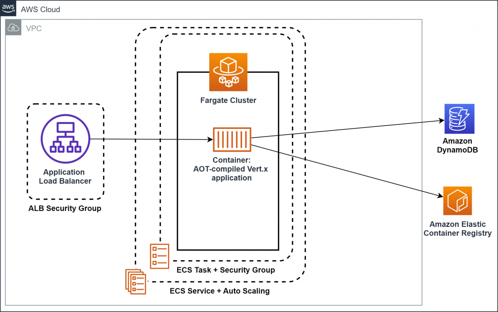
Customers are utilizing Fargate Spot for a wide variety of workloads, such as Monte Carlo simulations and genomic processing. In this blog, I utilize a python code with the Tensorflow library that can run as a container image in order to train a simple linear model. It runs the training steps in a loop on a data batch and periodically writes checkpoints to S3. If there is a Fargate Spot interruption, then it restores the checkpoint from S3 (when a new Fargate Instance occurs) and continues training. We will deploy this on AWS ECS Fargate Spot for low-cost, serverless task deployment utilizing CircleCI.
Concepts
Before looking at the solution, let’s revisit some of the concepts we’ll be using.
Capacity Providers: Capacity providers let you manage computing capacity for Amazon ECS containers. This allows the application to define its requirements for how it utilizes the capacity. With capacity providers, you can define flexible rules for how containerized workloads run on different compute capacity types and manage the capacity scaling. Furthermore, capacity providers improve the availability, scalability, and cost of running tasks and services on Amazon ECS. In order to run tasks, the default capacity provider strategy will be utilized, or an alternative strategy can be specified if required.
AWS Fargate and AWS Fargate Spot capacity providers don’t need to be created. They are available to all accounts and only need to be associated with a cluster for utilization. When a new cluster is created via the Amazon ECS console, along with the Networking-only cluster template, the FARGATE and FARGATE_SPOT capacity providers are automatically associated with the new cluster.
CircleCI Orbs: Orbs are reusable CircleCI configuration packages that help automate repeated processes, accelerate project setup, and ease third-party tool integration. Orbs can be found in the developer hub on the CircleCI orb registry. Each orb listing has usage examples that can be referenced. Moreover, each orb includes a library of documented components that can be utilized within your config for more advanced purposes. Since the 2.0.0 release, the AWS ECS Orb supports the capacity provider strategy parameter for running tasks allowing you to efficiently run any ECS task against your new or existing clusters via Fargate Spot capacity providers.
Solution overview
Fargate Spot helps cost-optimize services that can handle interruptions like Containerized workloads, CI/CD, or Web services behind a load balancer. When Fargate Spot needs to interrupt a running task, it sends a SIGTERM signal. It is best practice to build applications capable of responding to the signal and shut down gracefully.
This walkthrough will utilize a capacity provider strategy leveraging Fargate and Fargate Spot, which mitigates risk if multiple Fargate Spot tasks get terminated simultaneously. If you’re unfamiliar with Fargate Spot, capacity providers, or capacity provider strategies, read our previous blog about Fargate Spot best practices here.
Prerequisites
Our walkthrough will utilize the following services:
- GitHub as a code repository
- AWS Fargate/Fargate Spot for running your containers as ECS tasks
- CircleCI for demonstrating a CI/CD pipeline. We will utilize CircleCI Cloud Free version, which allows 2,500 free credits/week and can run 1 job at a time.
We will run a Job with CircleCI ECS Orb in order to deploy 4 ECS Tasks on Fargate and Fargate Spot. You should have the following prerequisites:
- An AWS account
- A GitHub account
Walkthrough
Step 1: Create AWS Keys for Circle CI to utilize.
Head to AWS IAM console, create a new user, i.e., circleci, and select only the Programmatic access checkbox. On the set permission page, select Attach existing policies directly. For the sake of simplicity, we added a managed policy AmazonECS_FullAccess to this user. However, for production workloads, employ a further least-privilege access model. Download the access key file, which will be utilized to connect to CircleCI in the next steps.
Step 2: Create an ECS Cluster, Task definition, and ECS Service
2.1 Open the Amazon ECS console
2.2 From the navigation bar, select the Region to use
2.3 In the navigation pane, choose Clusters
2.4 On the Clusters page, choose Create Cluster
2.5 Create a Networking only Cluster ( Powered by AWS Fargate)

This option lets you launch a cluster in your existing VPC to utilize for Fargate tasks. The FARGATE and FARGATE_SPOT capacity providers are automatically associated with the cluster.
2.6 Click on Update Cluster to define a default capacity provider strategy for the cluster, then add FARGATE and FARGATE_SPOT capacity providers each with a weight of 1. This ensures Tasks are divided equally among Capacity providers. Define other ratios for splitting your tasks between Fargate and Fargate Spot tasks, i.e., 1:1, 1:2, or 3:1.

2.7 Here we will create a Task Definition by using the Fargate launch type, give it a name, and specify the task Memory and CPU needed to run the task. Feel free to utilize any Fargate task definition. You can use your own code, add the code in a container, or host the container in Docker hub or Amazon ECR. Provide a name and image URI that we copied in the previous step and specify the port mappings. Click Add and then click Create.
We are also showing an example of a python code using the Tensorflow library that can run as a container image in order to train a simple linear model. It runs the training steps in a loop on a batch of data, and it periodically writes checkpoints to S3. Please find the complete code here. Utilize a Dockerfile to create a container from the code.
Sample Docker file to create a container image from the code mentioned above.
FROM ubuntu:18.04
WORKDIR /app
COPY . /app
RUN pip install -r requirements.txt EXPOSE 5000 CMD python tensorflow_checkpoint.py
Below is the Code Snippet we are using for Tensorflow to Train and Checkpoint a Training Job.
def train_and_checkpoint(net, manager):
  ckpt.restore(manager.latest_checkpoint).expect_partial()
  if manager.latest_checkpoint:
    print("Restored from {}".format(manager.latest_checkpoint))
  else:
    print("Initializing from scratch.")
  for _ in range(5000):
    example = next(iterator)
    loss = train_step(net, example, opt)
    ckpt.step.assign_add(1)
    if int(ckpt.step) % 10 == 0:
        save_path = manager.save()
        list_of_files = glob.glob('tf_ckpts/*.index')
        latest_file = max(list_of_files, key=os.path.getctime)
        upload_file(latest_file, 'pythontfckpt', object_name=None)
        list_of_files = glob.glob('tf_ckpts/*.data*')
        latest_file = max(list_of_files, key=os.path.getctime)
        upload_file(latest_file, 'pythontfckpt', object_name=None)
        upload_file('tf_ckpts/checkpoint', 'pythontfckpt', object_name=None)
2.8 Next, we will create an ECS Service, which will be used to fetch Cluster information while running the job from CircleCI. In the ECS console, navigate to your Cluster, From Services tab, then click create. Create an ECS service by choosing Cluster default strategy from the Capacity provider strategy dropdown. For the Task Definition field, choose webapp-fargate-task, which is the one we created earlier, enter a service name, set the number of tasks to zero at this point, and then leave everything else as default. Click Next step, select an existing VPC and two or more Subnets, keep everything else default, and create the service.
Step 3: GitHub and CircleCI Configuration
Create a GitHub repository, i.e., circleci-fargate-spot, and then create a .circleci folder and a config file config.yml. If you’re unfamiliar with GitHub or adding a repository, check the user guide here.
For this project, the config.yml file contains the following lines of code that configure and run your deployments.
version: '2.1'
orbs:
  aws-ecs: circleci/[email protected]
  aws-cli: circleci/[email protected]
  orb-tools: circleci/[email protected]
  shellcheck: circleci/[email protected]
  jq: circleci/[email protected]

jobs:

  test-fargatespot:
      docker:
        - image: cimg/base:stable
      steps:
        - aws-cli/setup
        - jq/install
        - run:
            name: Get cluster info
            command: |
              SERVICES_OBJ=$(aws ecs describe-services --cluster "${ECS_CLUSTER_NAME}" --services "${ECS_SERVICE_NAME}")
              VPC_CONF_OBJ=$(echo $SERVICES_OBJ | jq '.services[].networkConfiguration.awsvpcConfiguration')
              SUBNET_ONE=$(echo "$VPC_CONF_OBJ" |  jq '.subnets[0]')
              SUBNET_TWO=$(echo "$VPC_CONF_OBJ" |  jq '.subnets[1]')
              SECURITY_GROUP_IDS=$(echo "$VPC_CONF_OBJ" |  jq '.securityGroups[0]')
              CLUSTER_NAME=$(echo "$SERVICES_OBJ" |  jq '.services[].clusterArn')
              echo "export SUBNET_ONE=$SUBNET_ONE" >> $BASH_ENV
              echo "export SUBNET_TWO=$SUBNET_TWO" >> $BASH_ENV
              echo "export SECURITY_GROUP_IDS=$SECURITY_GROUP_IDS" >> $BASH_ENV=$SECURITY_GROUP_IDS=$SECURITY_GROUP_IDS" >> $BASH_ENV" >> $BASH_ENV
              echo "export CLUSTER_NAME=$CLUSTER_NAME" >> $BASH_ENV
        - run:
            name: Associate cluster
            command: |
              aws ecs put-cluster-capacity-providers \
                --cluster "${ECS_CLUSTER_NAME}" \
                --capacity-providers FARGATE FARGATE_SPOT  \
                --default-capacity-provider-strategy capacityProvider=FARGATE,weight=1 capacityProvider=FARGATE_SPOT,weight=1\                --region ${AWS_DEFAULT_REGION}
        - aws-ecs/run-task:
              cluster: $CLUSTER_NAME
              capacity-provider-strategy: capacityProvider=FARGATE,weight=1 capacityProvider=FARGATE_SPOT,weight=1
              launch-type: ""
              task-definition: webapp-fargate-task
              subnet-ids: '$SUBNET_ONE, $SUBNET_TWO'
              security-group-ids: $SECURITY_GROUP_IDS
              assign-public-ip : ENABLED
              count: 4

workflows:
  run-task:
    jobs:
      - test-fargatespot
Now, Create a CircleCI account. Choose Login with GitHub. Once you’re logged in from the CircleCI dashboard, click Add Project and add the project circleci-fargate-spot from the list shown.
When working with CircleCI Orbs, you will need the config.yml file and environment variables under Project Settings.
The config file utilizes CircleCI version 2.1 and various Orbs, i.e., AWS-ECS, AWS-CLI, and JQ. We will use a job test-fargatespot, which uses a Docker image, and we will setup the environment. In config.yml we are using the jq tool to parse JSON and fetch the ECS cluster information like VPC config, Subnets, and Security Groups needed to run an ECS task. As we are utilizing the capacity-provider-strategy, we will set the launch type parameter to an empty string.
In order to run a task, we will demonstrate how to override the default Capacity Provider strategy with Fargate & Fargate Spot, both with a weight of 1, and to divide tasks equally among Fargate & Fargate Spot. In our example, we are running 4 tasks, so 2 should run on Fargate and 2 on Fargate Spot.
Parameters like ECS_SERVICE_NAME, ECS_CLUSTER_NAME and other AWS access specific details are added securely under Project Settings and can be utilized by other jobs running within the project.
Add the following environment variables under Project Settings
-
- AWS_ACCESS_KEY_ID – From Step 1
- AWS_SECRET_ACCESS_KEY – From Step 1
- AWS_DEFAULT_REGION – i.e. : – us-west-2
- ECS_CLUSTER_NAME – From Step 2
- ECS_SERVICE_NAME – From Step 2
- SECURITY_GROUP_IDS – Security Group that will be used to run the task

Step 4: Run Job
Now in the CircleCI console, navigate to your project, choose the branch, and click Edit Config to verify that config.xml is correctly populated. Check for the ribbon at the bottom. A green ribbon means that the config file is valid and ready to run. Click Commit & Run from the top-right menu.
Click build Status to check its progress as it runs.

A successful build should look like the one below. Expand each section to see the output.

Return to the ECS console, go to the Tasks Tab, and check that 4 new tasks are running. Click each task for the Capacity provider details. Two tasks should have run with FARGATE_SPOT as a Capacity provider, and two should have run with FARGATE.
Congratulations!
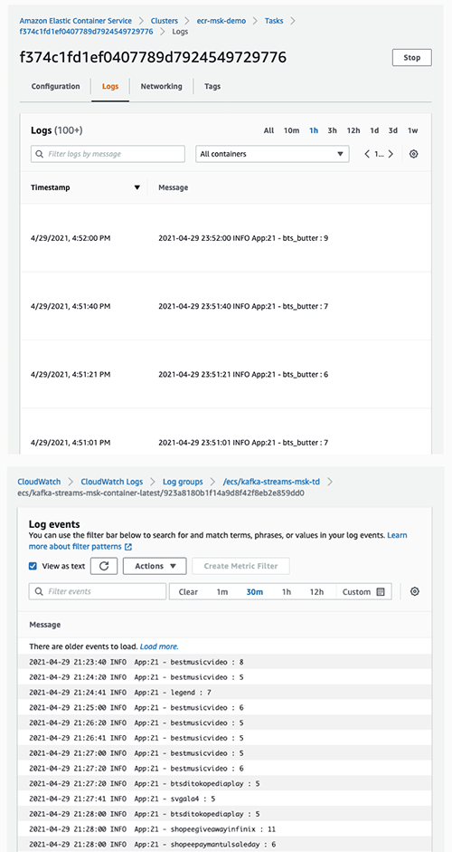
You have successfully deployed ECS tasks utilizing CircleCI on AWS Fargate and Fargate Spot. If you have used any sample web applications, then please use the public IP address to see the page. If you have used the sample code that we provided, then you should see Tensorflow training jobs running on Fargate instances. If there is a Fargate Spot interruption, then it restores the checkpoint from S3 when a new Fargate Instance comes up and continues training.
Cleaning up
In order to avoid incurring future charges, delete the resources utilized in the walkthrough. Go to the ECS console and Task tab.
- Delete any running Tasks.
- Delete ECS cluster.
- Delete the circleci user from IAM console.
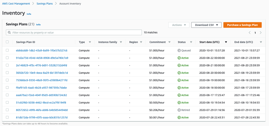
Cost analysis in Cost Explorer
In order to demonstrate a cost breakdown between the tasks running on Fargate and Fargate Spot, we left the tasks running for a day. Then, we utilized Cost Explorer with the following filters and groups in order discover the savings by running Fargate Spot.
Apply a filter on Service for ECS on the right-side filter, set Group by to Usage Type, and change the time period to the specific day.

The cost breakdown demonstrates how Fargate Spot usage (indicated by “SpotUsage”) was significantly less expensive than non-Spot Fargate usage. Current Fargate Spot Pricing can be found here.
Conclusion
In this blog post, we have demonstrated how to utilize CircleCI to deploy and manage ECS tasks and run applications in a cost-effective serverless approach by using Fargate Spot.
Author bio
 |
Pritam is a Sr. Specialist Solutions Architect on the EC2 Spot team. For the last 15 years, he evangelized DevOps and Cloud adoption across industries and verticals. He likes to deep dive and find solutions to everyday problems. |
 |
Dan is a Sr. Spot GTM Specialist on the EC2 Spot Team. He works closely with Amazon Partners to ensure that their customers can optimize and modernize their compute with EC2 Spot. |


 Florian Mair is a Solutions Architect at AWS.He is a t echnologist that helps customers in Germany succeed and innovate by solving business challenges using AWS Cloud services. Besides working as a Solutions Architect, Florian is a passionate mountaineer, and has climbed some of the highest mountains across Europe.