Post Syndicated from Benjamin Smith original https://aws.amazon.com/blogs/compute/serverless-icymi-q2-2023/
Welcome to the 22nd edition of the AWS Serverless ICYMI (in case you missed it) quarterly recap. Every quarter, we share all the most recent product launches, feature enhancements, blog posts, webinars, live streams, and other interesting things that you might have missed!

In case you missed our last ICYMI, check out what happened last quarter here.
Serverless Innovation Day

AWS recently hosted the Serverless Innovation Day, a day of live streams that showcased AWS serverless technologies such as AWS Lambda, Amazon ECS with AWS Fargate, Amazon EventBridge, and AWS Step Functions. The event included insights from AWS leaders such as Holly Mesrobian, Ajay Nair, and Usman Khalid, as well as prominent customers and our serverless Developer Advocate team. It provided insights into serverless modernization success stories, use cases, and best practices. If you missed the event, you can catch up on the recorded sessions here.
Serverless Land, your go-to resource for all things serverless, expanded to include a new Serverless Testing section. This provides valuable insights, patterns, and best practices for testing integrations using AWS SAM and CDK templates.
Serverless Land also launched a new learning page featuring a collection of resources, including blog posts, videos, workshops, and training materials, allowing users to choose a learning path from a variety of topics. “EventBridge Visuals“, small, easily digestible visuals focused on EventBridge have also been added.
AWS Lambda

Lambda introduced support for response payload streaming allowing functions to progressively stream response data to clients. This feature significantly improves performance by reducing the time to first byte (TTFB) latency, benefiting web and mobile applications.
Response streaming is particularly useful for applications with large payloads such as images, videos, documents, or database results. It eliminates the need to buffer the entire payload in memory and enables the transfer of responses larger than Lambda’s 6 MB limit, up to a soft limit of 20 MB.
By configuring the Function URL to use the InvokeWithResponseStream API, streaming responses can be accessed through an HTTP client that supports incremental response data. This enhancement expands Lambda’s capabilities, allowing developers to handle larger payloads more efficiently and enhance the overall performance and user experience of their web and mobile applications.
Lambda now supports Java 17 with Amazon Corretto distribution, providing long-term support and improved performance. Java 17 introduces new language features like records, sealed classes, and multi-line strings. The runtime uses ZGC and Shenandoah garbage collectors to reduce latency. Default JVM configuration changes optimize tiered compilation for reduced startup latency. Developers can use Java 17 in Lambda through AWS Management Console, AWS SAM, and AWS CDK. Popular frameworks like Spring Boot 3 and Micronaut 4 require Java 17 as a minimum. Micronaut provides a web service to generate example projects using Java 17 and AWS CDK infrastructure.
Lambda now supports the Ruby 3.2 runtime, enabling you to write serverless functions using the latest version of the Ruby programming language. This update enhances developer productivity and brings new features and improvements to your Ruby-based Lambda functions.
Lambda introduced support for Kafka and Amazon MQ event sources in four additional Regions. This expanded availability allows developers to build event-driven architectures using these messaging systems in more regions around the world, providing greater flexibility and scalability. It also supports Kafka and Amazon MQ event sources in AWS GovCloud (US) Regions, allowing government organizations to leverage the benefits of event-driven architectures in their cloud environments.
Lambda also added support for starting from a specific timestamp for Kafka event sources, allowing for precise message processing and useful scenarios like Disaster Recovery, without any additional charges.
Serverless Land has launched new learning paths for Lambda to help you level up your serverless skills:
- The Java Replatforming learning path guides Java developers through the process of migrating existing Java applications to a serverless architecture.
- The Lift and Shift to Serverless learning path provides guidance on migrating traditional applications to a serverless environment.
- Lambda Fundamentals is a 23-part video series providing practical examples and tips to help you get started with serverless development using Lambda.
The new AWS Tech Talk, Best practices for building interactive applications with AWS Lambda, helps you learn best practices and architectural patterns for building web and mobile backends as well as API-driven microservices on Lambda. Explore how to take advantage of features in Lambda, Amazon API Gateway, Amazon DynamoDB, and more to easily build highly scalable serverless web applications.
AWS Step Functions
The latest update to AWS Step Functions introduces versions and aliases, allows users to run specific state machine revisions, ensuring reliable deployments, reducing risks, and providing version visibility. Appending version numbers to the state machine ARN enables selection of desired versions, even after updates. Aliases distribute execution requests based on weights, supporting incremental deployment patterns.

This enhances confidence in state machine updates, improves observability, auditing, and can be managed through the Step Functions console or AWS CloudFormation. Versions and aliases are available in all supported AWS Regions at no extra cost.
AWS SAM
AWS SAM CLI has introduced a new feature called remote invoke that allows developers to test Lambda functions in the AWS Cloud. This feature enables developers to invoke Lambda functions from their local development environment and provides options for event payloads, output formats, and logging.

It can be used with or without AWS SAM and can be combined with AWS SAM Accelerate for streamlined development and testing. Overall, the remote invoke feature simplifies serverless application testing in the AWS Cloud.
Amazon EventBridge
EventBridge announced an open-source connector for Kafka Connect, providing seamless integration between EventBridge and Kafka Connect. This connector simplifies the process of streaming events from Kafka topics to EventBridge, enabling you to build event-driven architectures with ease.
EventBridge has improved end-to-end latencies for event buses, delivering events up to 80% faster. This enables broader use in latency-sensitive applications such as industrial and medical applications, with the lower latencies applied by default across all AWS Regions at no extra cost.
Amazon Aurora Serverless v2
Amazon Aurora Serverless v2 is now available in four additional Regions, expanding the reach of this scalable and cost-effective serverless database option. With Aurora Serverless v2, you can benefit from automatic scaling, pause-and-resume capability, and pay-per-use pricing, enabling you to optimize costs and manage your databases more efficiently.
Amazon SNS
Amazon SNS now supports message data protection in five additional Regions, ensuring the security and integrity of your message payloads. With this feature, you can encrypt sensitive message data at rest and in transit, meeting compliance requirements and safeguarding your data.
Serverless Blog Posts
April 2023
Apr 27 – AWS Lambda now supports Java 17
Apr 27 – Optimizing Amazon EC2 Spot Instances with Spot Placement Scores
Apr 26 – Building private serverless APIs with AWS Lambda and Amazon VPC Lattice
Apr 25 – Implementing error handling for AWS Lambda asynchronous invocations
Apr 20 – Understanding techniques to reduce AWS Lambda costs in serverless applications
Apr 18 – Python 3.10 runtime now available in AWS Lambda
Apr 13 – Optimizing AWS Lambda extensions in C# and Rust
Apr 7 – Introducing AWS Lambda response streaming
May 2023
May 24 – Developing a serverless Slack app using AWS Step Functions and AWS Lambda
May 11 – Automating stopping and starting Amazon MWAA environments to reduce cost
May 10 – Monitor Amazon SNS-based applications end-to-end with AWS X-Ray active tracing
May 10 – Debugging SnapStart-enabled Lambda functions made easy with AWS X-Ray
May 10 – Implementing cross-account CI/CD with AWS SAM for container-based Lambda functions
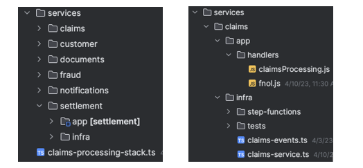
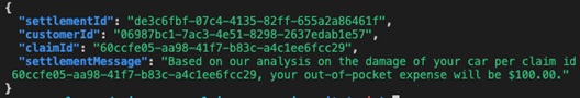
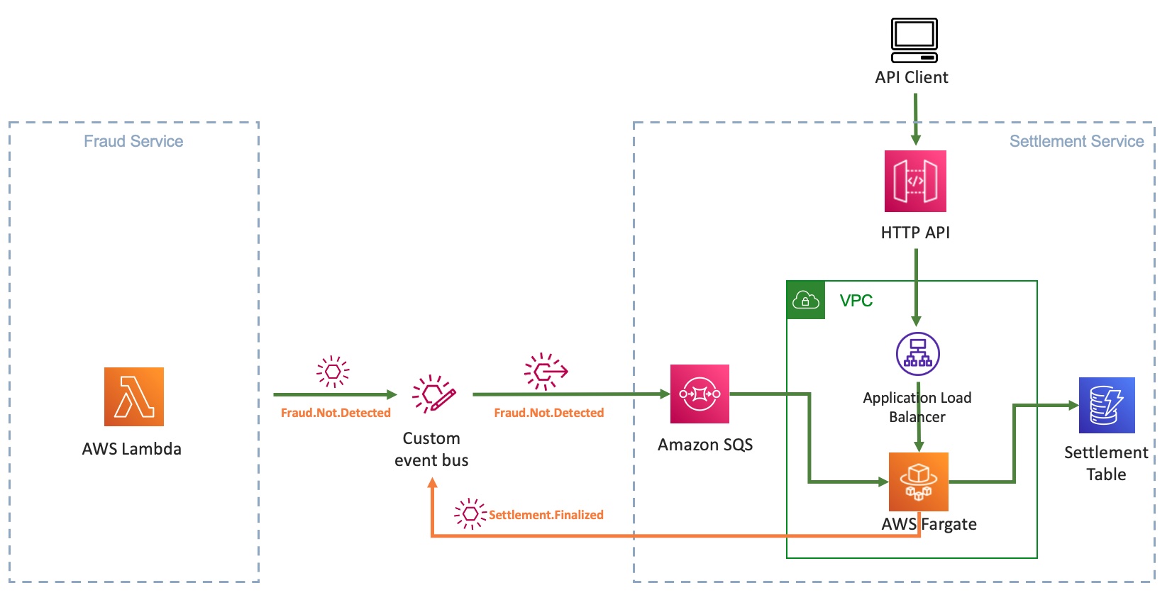
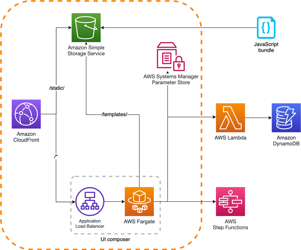
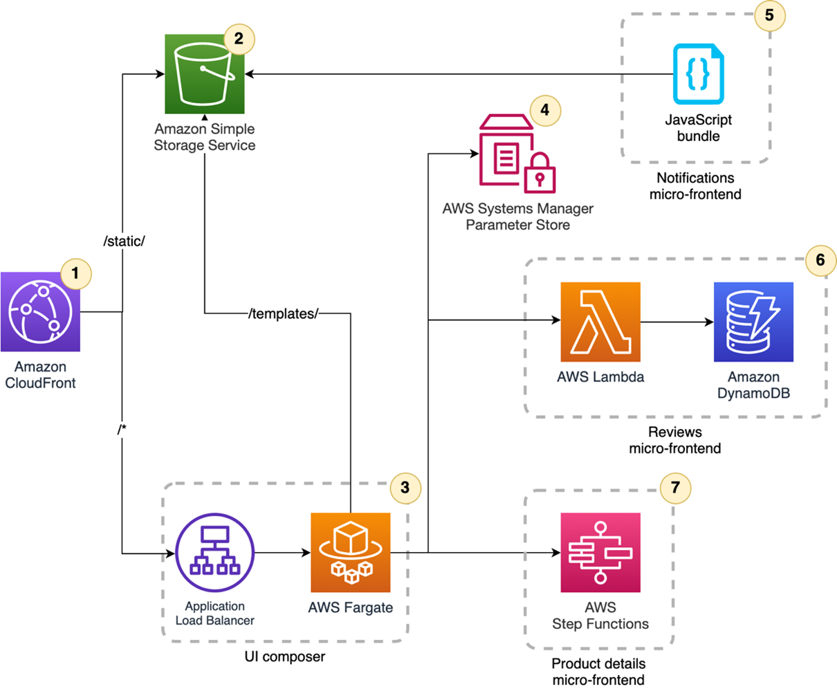
May 3 – Extending a serverless, event-driven architecture to existing container workloads
May 3 – Patterns for building an API to upload files to Amazon S3
June 2023
Jun 7 – Ruby 3.2 runtime now available in AWS Lambda
Jun 5 – Implementing custom domain names for Amazon API Gateway private endpoints using a reverse proxy
June 22 – Deploying state machines incrementally with versions and aliases in AWS Step Functions
June 22 – Testing AWS Lambda functions with AWS SAM remote invoke
Videos
Serverless Office Hours – Tues 10AM PT

Weekly live virtual office hours. In each session we talk about a specific topic or technology related to serverless and open it up to helping you with your real serverless challenges and issues.
YouTube: youtube.com/serverlessland
Twitch: twitch.tv/aws
LinkedIn: linkedin.com/company/serverlessland
April 2023
Apr 4 – Serverless AI with ChatGPT and DALL-E
Apr 11 – Building Java apps with AWS SAM
Apr 18 – Managing EventBridge with Kubernetes
Apr 25 – Lambda response streaming
May 2023
May 2 – Automating your life with serverless
May 9 – Building real-life asynchronous architectures
May 16 – Testing Serverless Applications
May 23 – Build faster with Amazon CodeCatalyst
May 30 – Serverless networking with VPC Lattice
June 2023
June 6 – AWS AppSync: Private APIs and Merged APIs
June 13 – Integrating EventBridge and Kafka
June 20 – AWS Copilot for serverless containers
June 27 – Serverless high performance modeling
FooBar Serverless YouTube channel
April 2023
Apr 6 – Designing a DynamoDB Table in 4 Steps: From Entities to Access Patterns
Apr 14 – Amazon CodeWhisperer – Improve developer productivity using machine learning (ML)
Apr 20 – Beginner’s Guide to DynamoDB with AWS CDK: Step-by-Step Tutorial for provisioning NoSQL Databases
Apr 27 – Build a WebApp that uses DynamoDB in 6 steps | DynamoDB Expressions
May 2023
May 4 – How to Migrate Data to DynamoDB?
May 11 – Load Testing DynamoDB: Observability and Performance tuning
May 18 – DynamoDB Streams – THE most powerful feature from DynamoDB for event-driven applications
May 25 – Track Application Events with DynamoDB streams and Email Notifications using EventBridge Pipes
June 2023
Jun 1 – How to filter messages based on the payload using Amazon SNS
June 8 – Getting started with Amazon Kinesis

Still looking for more?
The Serverless landing page has more information. The Lambda resources page contains case studies, webinars, whitepapers, customer stories, reference architectures, and even more Getting Started tutorials.
You can also follow the Serverless Developer Advocacy team on Twitter to see the latest news, follow conversations, and interact with the team.
- Eric Johnson: @edjgeek
- James Beswick: @jbesw
- Ben Smith: @benjamin_l_s
- Julian Wood: @julian_wood
- Marcia Villalba: @mavi888uy
- David Boyne: @boyney123