The story starts in 1996, when Matthias Ettrich, a student at the University
of Tübingen, posted to a Usenet group asking for programmers to help build a
desktop for Linux. What followed became KDE, one of the largest free software
communities in the world. KDE made Linux usable as a desktop for people who
weren’t system administrators, giving it a complete, consistent graphical
environment at a time when there was none.
The film covers the highs and lows of three decades of KDE: the Qt licensing
fight and the rivalry with GNOME; the success of KHTML, the browser engine that
became the basis of Apple’s WebKit and Google’s Chrome; and the contentious
release of KDE 4 and the rebuild that followed.
Ubuntu 26.10 advances enterprise security features, completes the rollout of
the Rust-based uutils coreutils, and strengthens integrations for user
authentication using Microsoft Entra ID.
[…] Ubuntu 26.10 also ships with GNOME 51, bringing a smoother, more
responsive desktop, better display handling, improved accessibility, and
refinements across core applications. In addition, the Ubuntu App Center now
provides a more consistent experience for managing snaps and debs.
Greg Kroah-Hartman has announced the release of the 7.2.11, 6.18.57, 6.12.113, 6.6.159, 6.1.190, 5.15.223, and 5.10.272 stable kernels. This series includes,
among other things, a fix for a
critical vulnerability (CVE-2026-99999). The
flaw in skb_checksum_help()
would allow an IPv4 packet with bad checksum metadata to “corrupt the network
header and cause a bunch of mischief” in the words of patch author Michael
S. Tsirkin. As usual, all users are advised to upgrade.
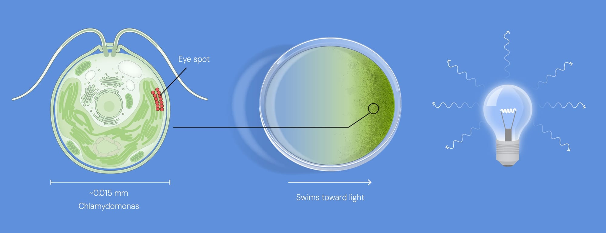
Историята започва с едно подвижно едноклетъчно водорасло, което има свойството да се насочва към светлината с помощта на двете си камшичета. Малките същества имат своеобразно „око“ (червеникаво петно на повърхността си), съдържащо ретинал – молекула, която може да улови енергията на светлината и да я превърне в химическа. Освен че са симпатични, едноклетъчните водорасли впечатляват с изключително бързата си реакция – електрическите импулси, които се генерират при осветяване на окото им, се отчитат само след половин милисекунда.
Това е изненада за Питър Хегеман, защото според разбирането към началото на 80-те години на миналия век процесът на обработка на тези импулси е по-бавен. Например в човешките очи светлината задейства сложна верига от различни молекули. Те си предават сигнала, докато след около 10 милисекунди той стигне до протеин, който може да образува специален отвор в клетъчната стена, т.нар. йонен канал. Специфичното е, че през него могат да преминат заредени частици (йони), предавайки малък електричен заряд на клетката. Това ѝ дава сигнал да се активира – така например работят невроните и мускулните клетки.
Хипотезата на Хегеман е, че най-вероятно активирането на йонните канали е следствие на по-прост процес, при който няма междинни стъпки, а каналите се контролират директно от светлината. За съжаление, към онзи момент са познати различни видове йонни канали, но не и контролирани от светлина, поради което идеята не бива приета.
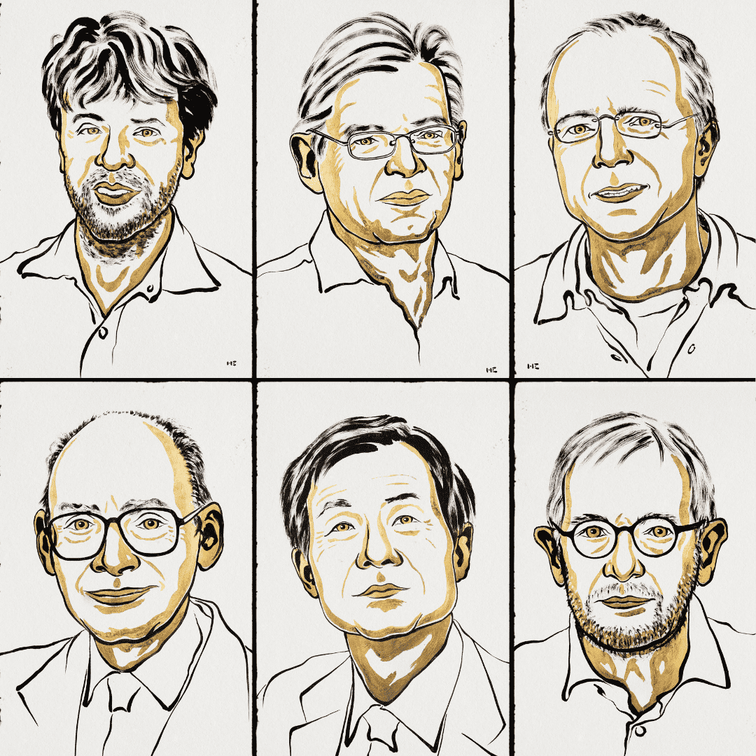
Хегеман не се отказва, но за следващата стъпка трябва да изчака няколко години, когато японски екип публикува генома на водораслото. С помощта на колегите си измежду всички гени той открива два, за които е много вероятно да кодират фоточувствителни протеини. За да потвърди, че това са търсените гени, Хегеман се свързва с Георг Нагел (с когото впоследствие ще сподели и Нобеловата награда), който има опит в изучаването на сходни протеини и разкриването на тяхната функция.
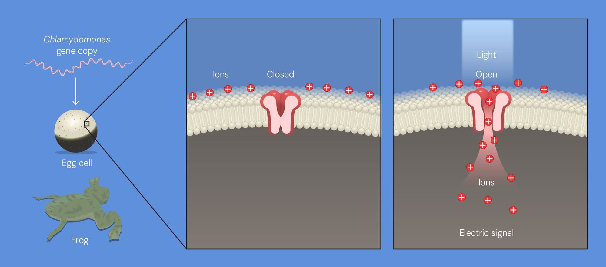
Експерименталната система, използвана от Нагел, са яйца от обикновената ноктеста жаба(Xenopus laevis). Ако в тях бъде вмъкната кодиращата последователност на някой ген, те могат да произведат неговия протеин, намножавайки го в лесна за наблюдение клетка. Когато бъдат внесени в яйцата, новите протеини се откриват по тънката им мембрана. След редица експерименти предположението на Хегеман се доказва – открити са нов вид йонни канали, които обикновено са затворени, но когато бъдат осветени, се отварят.
Експериментът е повторен и в клетки от бозайници (човек и хамстер), които също стават светлочувствителни. Двата протеина получават имената channelrhodopsin1 и 2(ChR1 и 2), като първият се активира от зелена светлина, а вторият е по-чувствителен към синя. Те се различават и по типа йони, които пропускат – ChR1 е селективен към протони (H+), а ChR2 пропуска всякакви положително заредени йони и при осветяването си генерира пик, след което поддържа по-нисък, но стабилен сигнал, ако светлината се задържи.
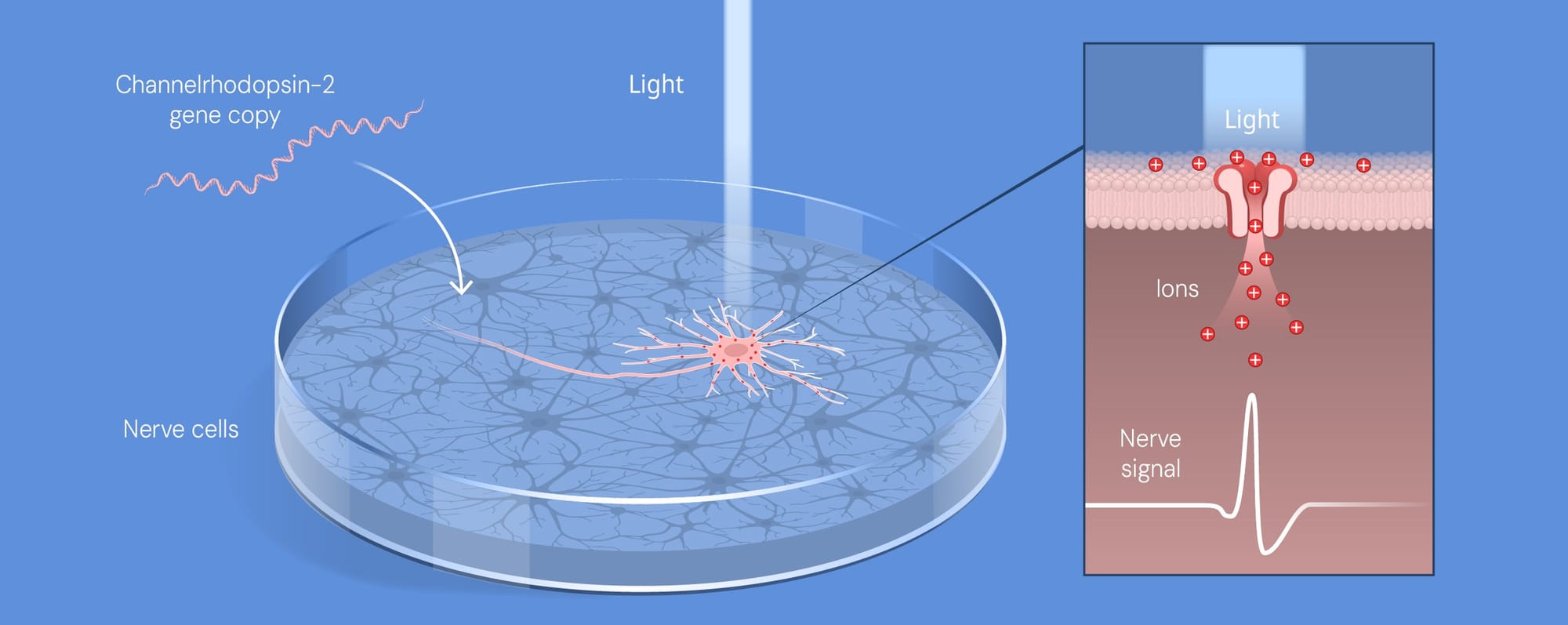
Публикацията на Нагел и Хегеман заинтригува Дайзерот, чийто екип се фокусира именно върху търсенето на начини за активиране на невронни клетки. След като получават копие от ChR2 от Нагел, Дайзерот и колегите му го вмъкват в неврони от плъх, които отглеждат като клетъчна култура. Въпреки първоначалните тревоги, че въвеждането на ген от водорасло в чувствителните нервни клетки ще наруши нормалната им работа, учените са приятно изненадани – след намесата няма видима вреда. Клетките не само се развиват нормално, но и придобиват нова способност: ако се осветят от синя светлина, те се активират, предавайки сигнала към съседните неврони. Този пробив поставя основата на ново научно поле, за чието съществуване се спекулира от Франсис Крик още в края на 70-те години на миналия век и което Дайзерот нарича оптогенетика.
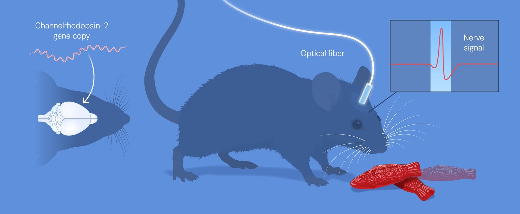
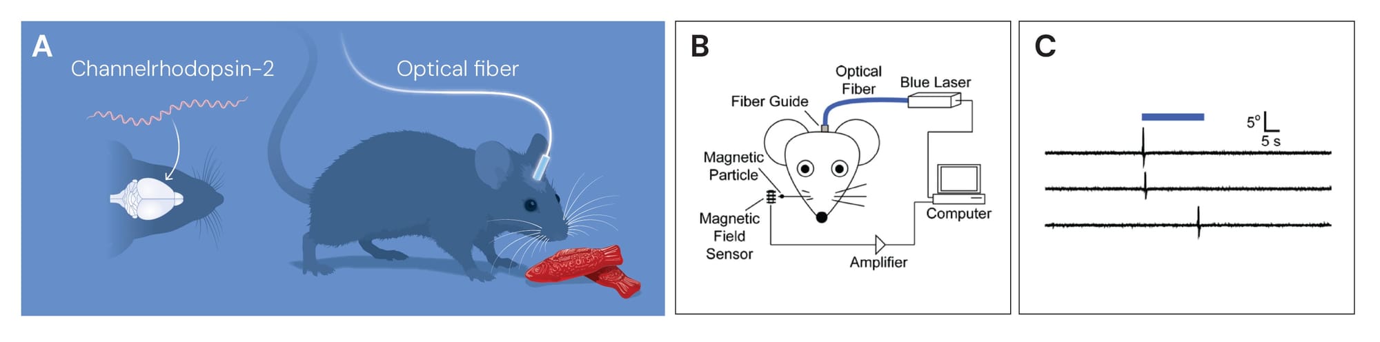
Светлинното активиране на неврони бързо се прехвърля от клетъчни култури към животни. Един от първите успешни експерименти на Дайзерот е стимулацията на невронни клетки в мозъка на мишки чрез тънка оптична нишка, прокарана през дупка в черепа им. ChR2 е вмъкнат в невронни клетки, специфични за двигателната кора на мозъка (частта, отговорна за движение), което дава възможност на учените да мърдат мустачките на мишката с помощта на син лазер.
Системата е използвана и за потвърждаване на функцията на нов вид мозъчни клетки, за които се подозира, че контролират състоянието на будност. След като учените ги модифицират и ги вмъкват обратно в мишки, с помощта на светлина мишките могат да бъдат събудени по команда и така се потвърждава очакваната роля на клетките.
Още по-впечатляващо е активирането на специфичен отпечатък върху невроните, появяващ се след създаване на спомен – т.нар. енграма. За целта първо мишките са изложени на среда, в която изпитват страх, като се отбелязват невроните, активни по това време. При светлинно активиране на тези неврони, дори и в спокойна среда, мишките дават същия стресов отговор. Експериментът е повторен при променени условия, като се създава „фалшив спомен“. Стресовите неврони се активират изкуствено в спокойна среда, след което при поставяне на животните в същата ситуация, те се страхуват, без да има причина.
В следващите години технологията се развива значително. Открити са нови протеини, които реагират при други цветове на светлината, давайки възможност за подаване на няколко сигнала едновременно. Това разширява значително възможността за изследване на мозъка и позволява да се определят специализациите на отделните невронни клетки и да се разплитат сложните взаимовръзки между тях. Така са открити невронни групи, които отговарят за усещането на болка, различни социални поведения, жажда, глад и регулация на сложни функции като циркаден ритъм и вдигането на температура при задействане на имунната система.
Освен разкритите възможности за фундаменталната наука, оптогенетиката има потенциал и за медицината. Като се използват знанията от изследвания върху различни психологични и неврологични заболявания, като депресия, тревожност, шизофрения, алцхаймер и паркинсон, е възможно в бъдеще да се създадат устройства, които да регулират невроните, отговорни за заболяването, с идеята да се намалят симптомите.
Надежда има и за подобряване на кохлеарните импланти, които в момента използват електрически сигнали, за да стимулират звуковите нерви. Ако това може да се прави със светлина, активирането на нервните клетки ще бъде много по-прецизно. В момента се провеждат и клинични изпитвания за терапия на слепи пациенти, като вече има положителни резултати с частично връщане на зрението.
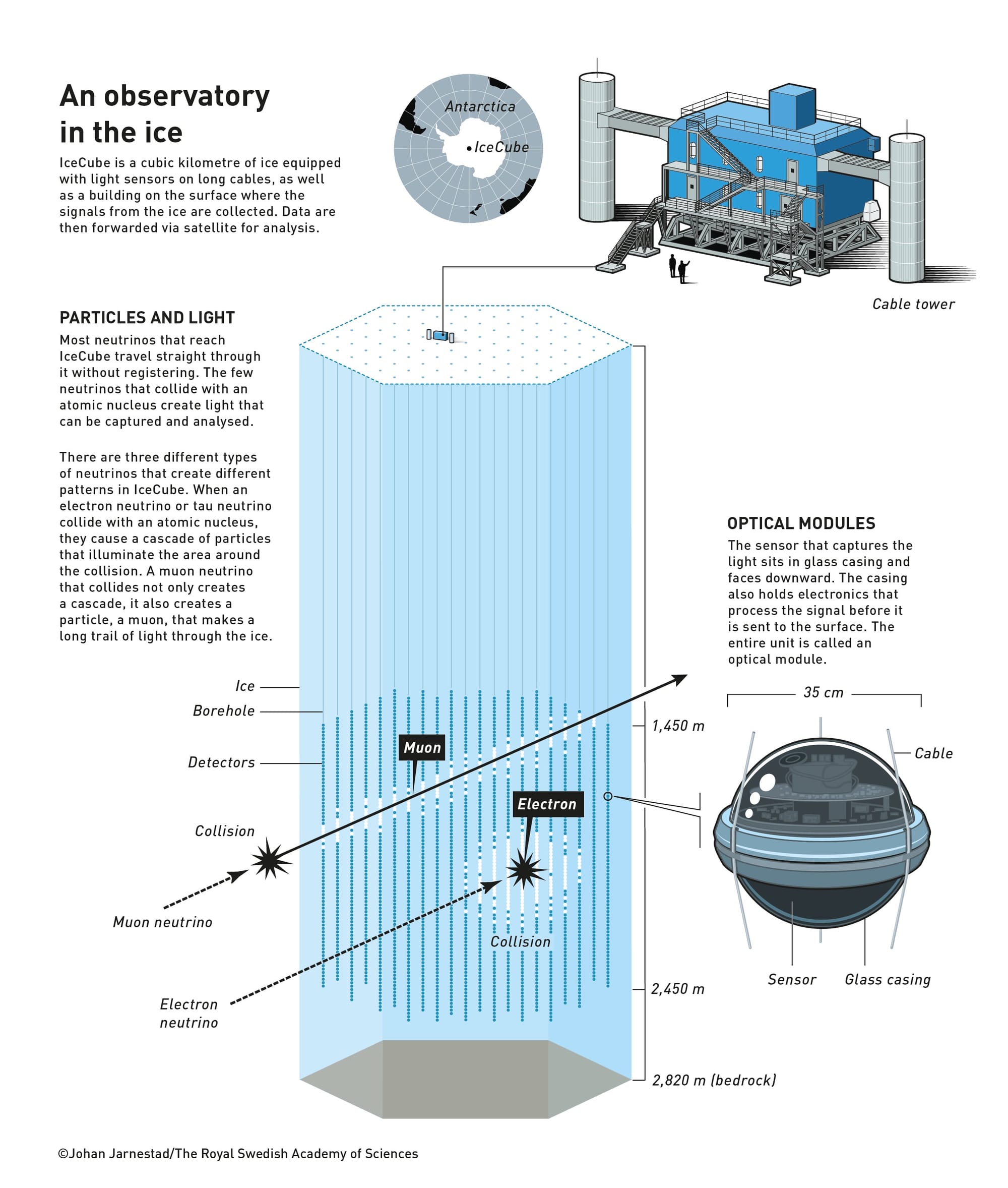
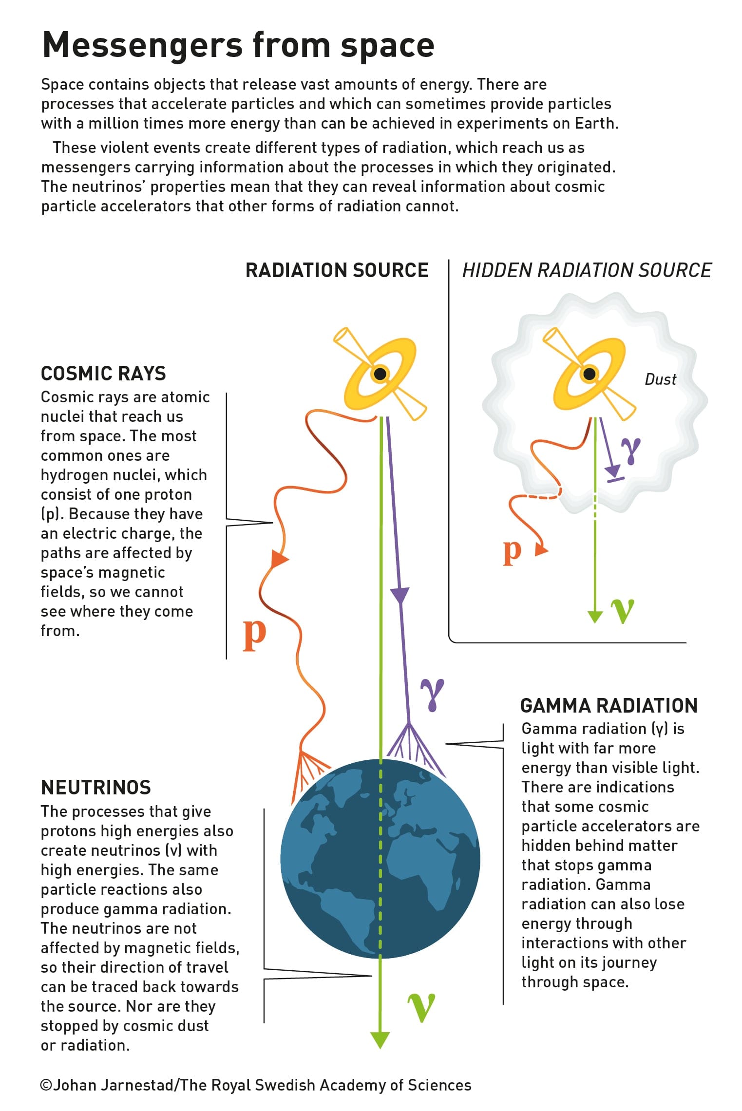
Неутриното е изключително интересна елементарна частица, която през повечето време лети през пространството със скорост, близка до тази на светлината. То няма електричен заряд, а масата му е пренебрежима, което му дава възможност да преминава през всички препятствия по пътя си, откъдето идва и прозвището му „призрачна частица“, популяризирано от Айзък Азимов. Естествените му източници са различни видове радиоактивен разпад и ядрени реакции, като протичащите в звездите или при експлозии на свръхнови, но може да се генерира също в ядрените реактори и в ускорителите на частици.
Призрачните свойства правят частиците неутрино изключително трудни за изучаване, въпреки че са сред най-разпространените във Вселената – всяка секунда през нокътя на малкия ви пръст преминават около 65 милиарда неутрино, идващи от Слънцето. Но именно защото не взаимодействат с материята, са интересни за учените – тяхната траектория и заряд остават на практика непроменени от момента на напускане на източника си и могат да дадат информация за него.
Частицата е „видяна“ за първи път през 1956 г. благодарение на напредъка в развитието на атомната енергетика, а малко по-късно е засечено и първото неутрино, излъчено от Слънцето. Но учените срещат проблем – засечените частици са много по-малко от теоретично очакваните. Подсказка защо това е така, идва през 1962 г., когато е открит нов тип неутрино (мюон неутрино), а пълният отговор е разкрит почти 40 години по-късно, когато през 2000 г., е открит и третият тип – тау неутрино. Междувременно е установено също, че частиците могат да сменят типа си по време на необезпокояваното си пътешествие – например един път са мюон, друг път са тау неутрино.
През годините има различни предложения за най-добрия метод за „лов“ на неутрино. Някои физици предлагат използването на големи водни басейни – когато неутрино се сблъска с атомно ядро, се образува заредена частица, която продължава в първоначалната посока на движение, но отделя светлина благодарение на ефекта на Черенков. Това би позволило да се види пътят на неутриното, но и да се определи откъде е дошло. Друга идея е използването на радиоантени, които да „слушат“ за тези сблъсъци, но вместо вода средата да е антарктическият лед.
Тук идва приносът на Халзен: той предлага двете идеи да се комбинират, като се използват фоточувствителни детектори, които да се поставят в дебелия лед на Южния полюс. Идеята му има редица силни страни. На Антарктида вече се води изследователска дейност, дебелият лед е стабилен материал, който е тъмен след определена дълбочина и за разлика от океаните няма обитатели, които да пречат на оборудването. Известен недостатък е трудният достъп, който е възможен само през краткото антарктическо лято.
Така започва работа по пилотна обсерватория, наречена AMANDA. В началото изследователите срещат пречка – в леда има малки мехурчета, които разпръскват светлината от частиците и маскират посоката им. Това кара учените да поставят сензорите по-дълбоко. След преминаването на 1400 метра попадат на изключително чист и хомогенен лед, в който проблясъците могат да пропътуват над 300 метра, преди да угаснат, а това е доста по-далеч от очакваното. Въпреки че обсерваторията работи добре, размерът ѝ се оказва недостатъчен за улавяне на неутрино с много голям заряд, идващи от далечни космически обекти. Потвърждението, че технологията работи, дава зелена светлина за започване на работа по следващата обсерватория. Мащабът на наследника, наречен IceCube, е наистина впечатляващ – детекторът е с обем от 1 кубичен километър, в който на дълбочина между 1450 и 2450 метра са поставени 5160 сензора.
Обсерваторията бързо дава резултат, засичайки частици, които идват от Дълбокия космос. През 2013 г. са засечени 37 неутрино с такъв произход, като три от тях носят изключително висока енергия и са наречени Бърт, Ърни и Голямото пиле (на героите от „Улица Сезам“). Четири години по-късно е уловено неутрино, което е проследено до източника си – блазараTXS 0506+056, който се намира на 3,7 млрд. светлинни години в посока съзвездието Орион. Други две частици пък идват от разкъсването на звезда от черна дупка. А през 2022 г. има новини за открит източник на неутрино в сърцевината на галактиката Messier 77, което дава нова информация за процесите, протичащи в активните галактически ядра.
Работата на обсерваторията продължава и в последните три години са добавени още 600 детектора. Макар че резултатите са добри, Халзен не спира да мечтае и да се надява, че ще бъдат направени още по-вълнуващи открития, които дори могат да бъдат извън очакваното според стандартния модел.
Когато получава новината за наградата, Халзен вече работи по предложение за нов проект и шеговито отбелязва: „Надявам се, че Нобелът ще помогне да го одобрят.“
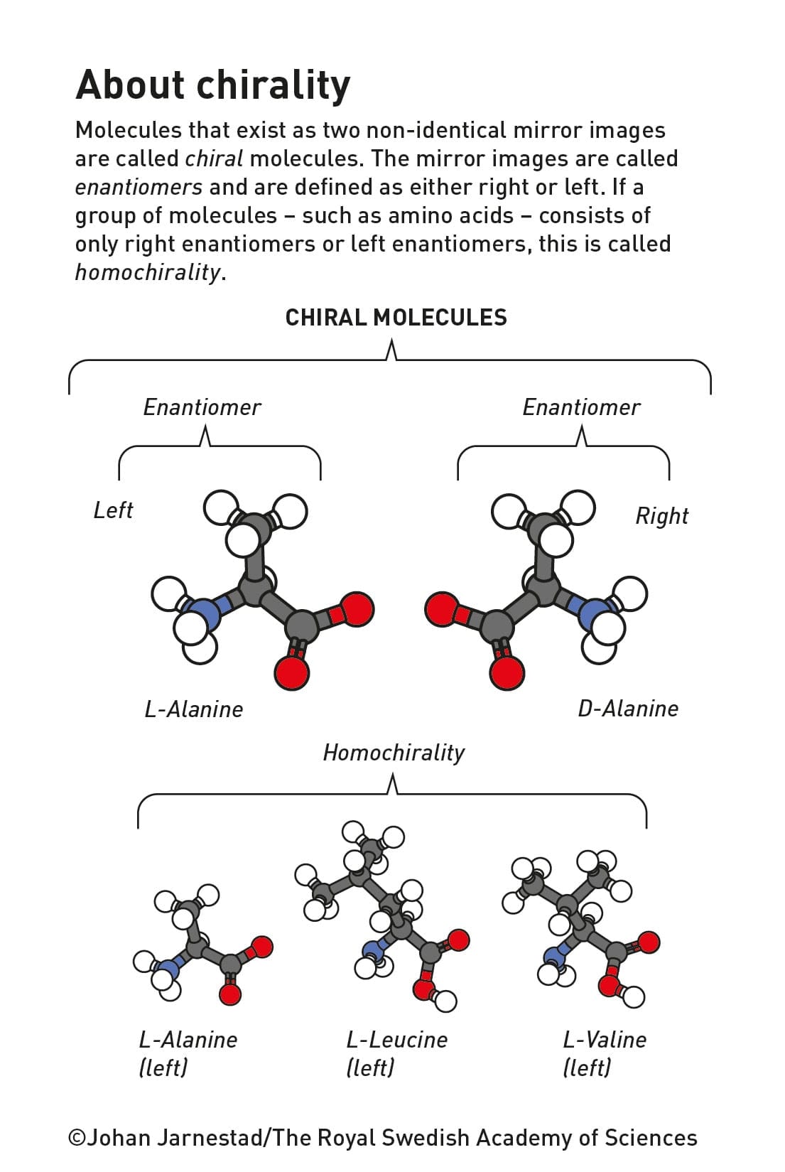
От някои химични реакции се получават две почти идентични молекули, които са огледални една на друга. Сред първите учени, обърнали внимание на феномена, е Луи Пастьор, който дочува от колеги, че понякога винената киселина изкривява поляризираната светлина, а понякога – не. Той се захваща да направи кристали от киселината и наблюдавайки ги под микроскоп, установява, че те имат два огледални варианта, които, ако бъдат разделени и разтворени поотделно, наистина могат да насочат светлината или наляво, или надясно. А когато двете се смесят, светлината не променя посоката си. Веществата, които имат такава способност, биват наречени хирални, а отделните им форми – енантиомери.
Пастьор прави и следващото интересно откритие: бактериите могат да разграждат дясновъртящата винена киселина в гроздето, но изобщо не проявяват интерес към другата форма. Това подсказва, че живите организми имат способността да различават двата варианта. По някаква причина животът на планетата се е развил по хомохирален начин – с използване само на едната форма на веществата. Например аминокиселините, които изграждат белтъците, винаги са лявовъртящи, а захарите – дясновъртящи.
Естественият въпрос е „Защо?“. Какво и как се е случило в зачатъка на живота, което да зададе едната или другата посока? Загадката е голяма, тъй като обикновено от химичните реакции се получават равни количества от двата хирални продукта. Тоест ако се опитаме да синтезираме винена киселина в лабораторията, крайният продукт няма да върти поляризираната светлина, защото ще е равна смес от двете форми. По някакъв неясен начин в гроздето се получава само дясна форма.
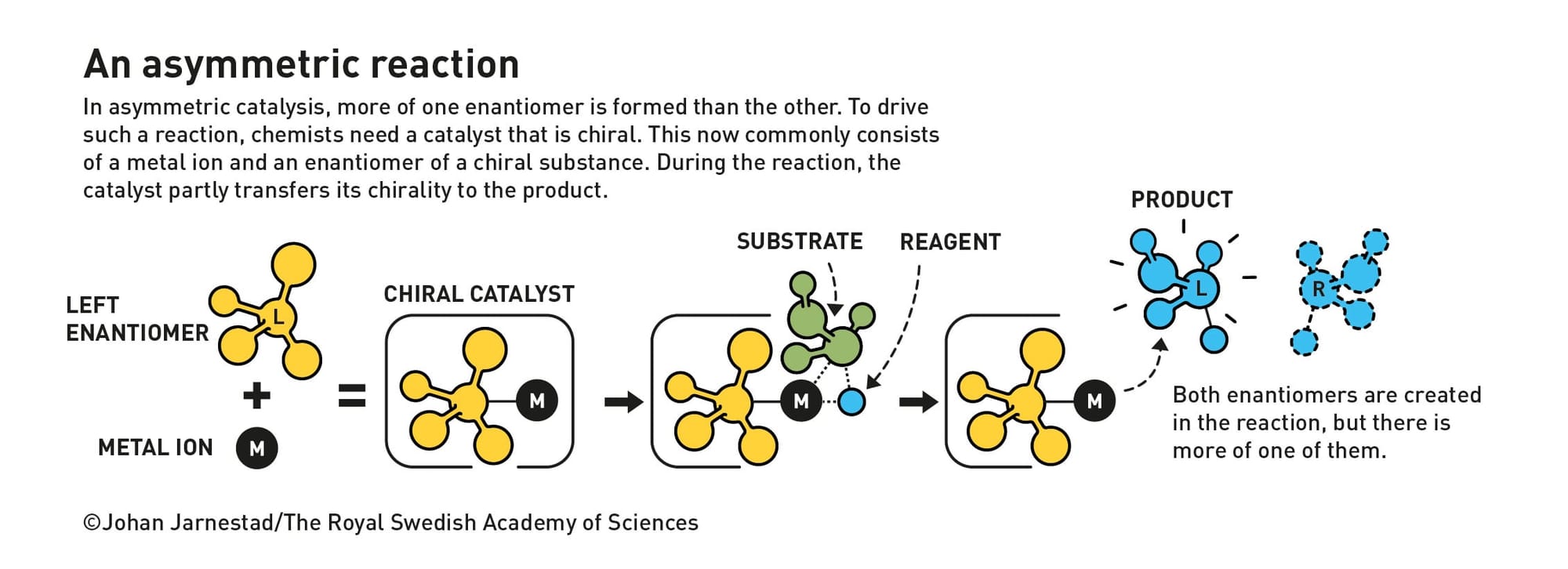
Един от първите пробиви по пътя към разгадаването на мистерията идва след откриването на първата асиметрична реакция (при която единият енантиомер се натрупва с предимство) с помощта на хирален катализатор. Неговата хиралност насочва реакцията към едната посока. Ефектът е минимален, но възможността за промяна на съотношението между двата енантиомера дава надежда на учените, че това има как да стане и в лабораториите, а не е някаква тайна, известна само на живите организми. С времето асиметричният синтез е подобрен, като дава много по-добър добив от желаната форма (дясна или лява), което донася и Нобелови награди за химия на учените, поставили основите през 2001 и 2021 г.
Работата на Каган е продължение на тяхната – получаването на възможно най-чисти молекули. Това е от особена важност при производството на медикаменти, защото понякога едната форма на веществата не е просто неактивна, а е вредна за организма.
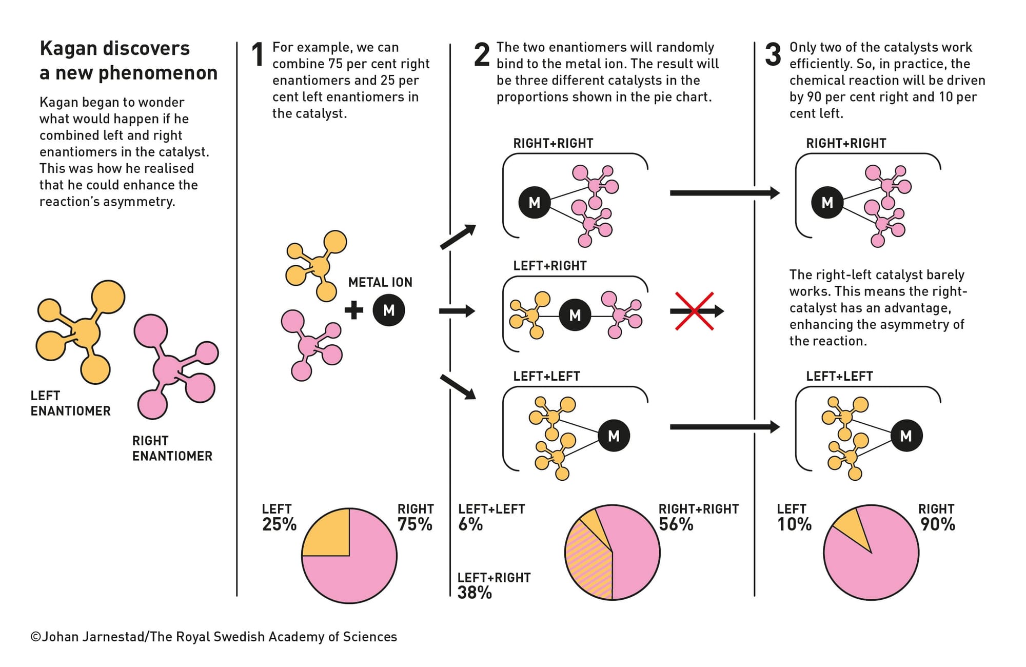
По това време учените мислят, че съотношението на двете версии на катализатора ще се предаде директно на продуктите от реакцията – хипотеза, която Каган поставя под съмнение, и той прави ново предположение. То се базира на факта, че катализаторите, които се използват в тези реакции, съдържат два компонента – метален атом, който е „двигателят“, и хирална молекула, която задава посоката. Идеята на Каган е, че към един метален атом могат да се прикрепят поне две хирални молекули и така се получават три версии на катализатора – ляво–ляво, ляво–дясно и дясно–дясно.
Докато двата еднопосочни катализатора дават очакваната молекула, съответно лява или дясна, смесеният не само че не работи на случаен принцип (да дава ту лява, ту дясна), а въобще не работи. Това означава, че ако се започне със 75% десен и 25% ляв катализатор, то ефективното съотношение е всъщност 90% към 10%, тъй като смесеният не работи. Този феномен се нарича нелинеен ефект.
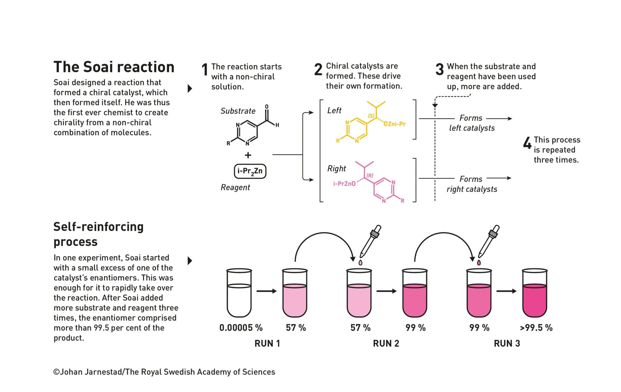
Соай задава следващия голям въпрос: възможно ли е да има асиметрична реакция, която сама да произвежда своя катализатор? След няколко години работа отговорът е положителен. Като се започва с около 2% повече от единия енантиомер на едно вещество, след няколко реакции то се концентрира до 87%. Постигната е първата автокаталитична асиметрична реакция. Успехът не спира Соай, който си поставя още по-амбициозна цел: да постигне пълната хомохиралност, която се наблюдава в природата. Това става след още 8 години – започва се с много малък превес на едната форма, а крайният продукт е съставен почти само от нея. Ако реакцията се остави на случайността, то крайният продукт е този, който е успял да вземе минимална преднина в началото.
Макар и изцяло синтетична, реакцията на Соай дава надежда на учените, че разкриването на тайната на хомохиралността при живите организми е възможна. Откритията на Каган и Соай имат голяма практическа важност, защото позволяват синтеза на изключително чисти медикаменти, пестициди и други вещества, които се прилагат върху живи организми. Нобелът е признание и за предаването на знания в науката, давайки възможност експерименталната нишка да се проследи до един от пионерите на биологията – бележития Луи Пастьор.
Веднъж месечно Михаил Ангелов – биолог, агроном и любим нърд от нашия екип, ни представя най-интересните скорошни новини от различни сфери на науката и обяснява защо тези постижения са толкова значими за света и човечеството. Или най-малкото – любопитни и забавни.
Предупреждение: Тази статия съдържа детайли, които може да се възприемат като разстройващи.
Какво е отношението ви към смъртното наказание? Ще ви разкажа как се формира моето.
На 5–6-годишна възраст живеех със семейството си в Бенгази, Либия. По онова време диктатурата на Муамар Кадафи беше още в разцвета си. Либия беше икономически доста по-напреднала от България. Помня тъмния и блестящ асфалт на улиците (никога дотогава не бях виждала такъв) и изобилието от западни стоки в магазините.
Сред нещата, запечатали се в паметта ми от либийския период, са и екзекуциите. Там бесеха хора на площадите и излъчваха това по телевизията. Гледаш си „Пчеличката Мая“ (в Либия пчеличката се наричаше Зина) и в следващия момент – хоп – екзекуция. На площада с бесилото – множество от екзалтирани възрастни и деца. Гледката на отнемането на човешки живот ме разстройваше – всеки път избухвах в плач и дълго време не можех да се успокоя. Ужасяваше ме както фактът, че някой умира, така и реакцията на тълпата зяпачи. Благодарна съм, че баща ми беше твърдо против и ние да ходим да гледаме.
Последната екзекуция в България
е извършена в самия край на тоталитарния период – в началото на ноември 1989 г. Престъпленията на убития чрез разстрел мъж, квалифицирани като диверсия, са серия от саботажи, сред които и повреждане на лифта на Боровец три пъти, защото държавата му пречела да развива частен бизнес като дърводелец.
След промените, още през 1990 г., се налага мораториум върху смъртното наказание, а в началото на 1999 г. то е изцяло премахнато. Няколко години по-късно, през 2002 г., повече от половината анкетирани в проучване на „Алфа Рисърч“ посочват, че са за възстановяването на смъртната присъда. Проучването е част от социален експеримент по идея на Центъра за либерални стратегии. Близо 300 от 1200-те респонденти са поканени да участват в дебат по темата, организиран от bTV, който включва юристи, експерти, но и пострадали от престъпления. В резултат на дискусиите 20% са променили позицията си от за екзекуциите на против тях. Изводът от социалния експеримент е, че обществото може да се вслушва в аргументи, ако такива му се предоставят.
Последното изследване за отношението към смъртното наказание е проведено от „Галъп“ през 2016 г. – близо 20 години след влизането на България в ЕС, където смъртно наказание не се прилага. Точно една трета се обявяват в защита на връщането му, докато близо половината (47%) са против. Но тези резултати са преди консервативния обрат, който започна да настъпва в България през 2018 г. с дезинформационната кампания срещу Истанбулската конвенция.
Смъртното наказание в САЩ и прецедентът с Криста Пайк
В ЕС е в сила пълна забрана на смъртното наказание – по силата на Протокол №13 към Конвенцията за защита на правата на човека и основните свободи, според който то се отменя, и чл. 2, ал. 2 от Хартата на основните права:
Никой не може да бъде осъден на смърт, нито екзекутиран.
В САЩ обаче смъртното наказание съществува в 27 от 50 щата, макар да не се прилага във всички тях. Американският президент Доналд Тръмп е толкова убеден привърженик на екзекуциите, че още в първия ден от встъпването си във втория мандат отмени наложения от предшественика му Джо Байдън мораториум върху изпълнението им на федерално равнище. Мораториумът на федерално ниво обаче не означава, че смъртни присъди не са се изпълнявали на щатско равнище. Федералното законодателство и щатските законодателства са различни системи, а присъдите на федерално равнище са за по-сериозни престъпления, например тероризъм.
Методите за екзекуция, които се прилагат в САЩ, са смъртоносни инжекции, електрически стол, разстрел, а от 2024 г. за първи път в света се въвежда нов метод – азотна хипоксия.
Пайк е осъдена на смърт в щата Тенеси още преди 31 години, защото на 18-годишна възраст е убила момиче, което според нея е искало да отнеме приятеля ѝ. Въпросният приятел също участвал в убийството, но се „отървал“ с доживотен затвор, защото е бил на 17 години. Още едно момиче е присъствало на убийството, но няма доказателства, че е участвало активно, затова е осъдено само условно.
За Криста Пайк също са налице смекчаващи вината обстоятелства: тя е преживяла нееднократно физическо и сексуално насилие, била е неглижирана като дете, на 12 години е направила опит за самоубийство. Диагностицирана е с няколко психически заболявания: биполярно и тежко посттравматично стресово разстройство и клинична депресия; има вродено мозъчно увреждане, което вероятно е свързано с биполярното ѝ разстройство и с (не)способността ѝ да прави преценка.
Ала нищо от това не променя убеждението на съда, че тийнейджърката трябва да заплати за стореното със собствената си смърт. След множество обжалвания и отлагания екзекуцията е изпълнена на 30 септември 2026 г. чрез инжектиране на пентобарбитал.
Криста Пайк обаче не умира.
И преди се е случвало екзекуция чрез инжекция да е неуспешна, но това е ставало основно защото палачите не са успявали да улучат вена на осъдените. Понеже на медицинските лица е забранено да изпълняват смъртни присъди, затворническият персонал се справя… както може.
През 2009 г. например екзекуторите два часа се опитват да вкарат игла във вените на Ромел Блум и го набождат на 18 места, докато той плаче от болка. Не успяват, а Блум умира 11 години по-късно от ковид, преди да е насрочена нова дата за умъртвяването му. Проблем има и с вените на Клейтън Локет – екзекуторите го бодат от 18:23 до 18:56 ч., вкарват игла дори в слабините му. Минути след като опитът за екзекуция е отменен, човекът умира – от инфаркт.
През 2018 г. бодат болния от лимфом Дойл Хам повече от два часа и така и не откриват вена. След това щатът (Алабама) взема решение да не прави нови опити да го убие. Алън Милър, чиято екзекуция през 2022 г., отново в Алабама, се проваля след часове убождания в търсене на вена, не изважда този късмет. Наказанието му е изпълнено успешно през 2024 г. – това е вторият случай на екзекуция чрез азотна хипоксия. На теория смъртта би трябвало да е бърза и неусетна – осъденият вдишва азот през маска и не усеща, че се задушава, а има чувството, че диша нормален въздух. На практика обаче, умирайки, Алън Милър видимо (според свидетели) се е мъчил.
За разлика от тези случаи, обявени за провалени, екзекуцията на Криста Пайк е изпълнена докрай.
Единственият подобен прецедент е от 1946-та с 16-годишния Уили Франсиз, осъден на смърт чрез електрически стол. Екзекуцията е извършена, но електричеството не е достатъчно силно и момчето остава живо. Върховният съд постановява присъдата да се изпълни отново с аргумента:
Стават инциденти, за които никой не е виновен.
Причините за неуспешното изпълнение на наказанието на Криста Пайк тепърва ще се изясняват. Адвокатите ѝ са убедили съда да изиска всички налични доказателства по случая. Но отсега се знае, че екзекуторите и в нейния случай се затрудняват да улучат вените. Опитват с поне седем игли и накрая май не успяват – веществото вероятно не влиза в кръвта на осъдената, а се разтича в тъканите ѝ.
На теория екзекуцията с пентобарбитал би трябвало да е бърза и безболезнена – човек се унася за секунди и дишането спира. Невинаги обаче става така. Криста Пайк усеща не само че многократно я бодат, а и как пентобарбиталът влиза в тялото ѝ. За да остане активното вещество в течно състояние, то трябва да е в силен алкален разтвор. Тоест нещо като белина. Или сода каустик.
Резултатът е болезнено химическо изгаряне. Свидетели на екзекуцията са чули Пайк да казва, че ръката ѝ гори толкова силно, сякаш всеки момент ще избухне.
След като първата доза, вкарана в лявата ѝ ръка, не я убива, прилагат втората в дясната. По закон след неуспех първия път може да се постави нова инжекция, но законът не предвижда друг опит, ако и вторият не е успешен. Час след началото на екзекуцията Криста Пайк е още жива и издава хрипове. Тогава служител на затвора се обажда на „Бърза помощ“ и след известни перипетии (диспечерите първоначално не са били сигурни, че сигналът е истински), жената е откарана в болница.
След няколко дни Криста Пайк се събужда, макар адвокатите ѝ да са били убедени, че е в мозъчна смърт. Пита: „Къде съм и кои сте вие?“ Изгарянията от разтвора с пентобарбитал са сериозни и тя не може да движи ръцете си, не е в състояние и да преглъща. Първоначално е объркана, но бързо се възстановява, започва да става и да се храни. През цялото време е с белезници и под охрана.
За успокоение на данъкоплатците скоро състоянието на Криста Пайк се подобрява дотолкова, че тя е върната в затвора, където е прекарала три от петте десетилетия на живота си. Но продължава да е под лекарско наблюдение.
След неуспешната ѝ екзекуция изпълнението на смъртни присъди в Тенеси е спряно до края на 2026 г. Не е сигурно дали ще има нов опит за прилагане на наказанието ѝ. Адвокатите на Пайк, както и правозащитници и противници на смъртното наказание се позовават на Осмата поправка в Конституцията на САЩ от 1791 г., според която няма да се „изпълняват жестоки и необичайни наказания“. Това, на което е била подложена Пайк, е и необичайно, и жестоко.
Ала силни са и гласовете, според които Криста Пайк заслужава да умре, защото е отнела човешки живот. Сред тях са майката на Колийн Слемър – убитото от Пайк момиче, и сенаторката от щата Тенеси, републиканката Марша Блекбърн. Трябва да имаме предвид, че в САЩ смъртното наказание се радва на високо одобрение – според различни изследвания от последните година-две 52% от американците го смятат за морално приемливо, а 66% го одобряват по отношение на осъдени за убийство.
Екзекуцията като риалити шоу
В разгара на дискусиите за и против смъртното наказание след неуспешната екзекуция на Криста Пайк министърът на войната на САЩ Пийт Хегсет предложи екзекуция чрез разстрел да се излъчва на живо по интернет. Става дума за изпълнението на смъртното наказание на Нидал Хасан, бивш военен, убил 13 невъоръжени военнослужещи през 2009 г. Въпреки че според близо 90% от водещите американски криминолози смъртното наказание не предотвратява извършването на убийства, според Хегсет целта на предаването на екзекуцията онлайн е хората да разберат, „че подобни действия имат сериозни последици“.
Тръмп одобрява планирания за началото на декември 2026 г. разстрел на Хасан, но до този момент не е дал съгласието си за излъчване онлайн.
Ако излъчването все пак се състои, САЩ, доскорошният „лидер на демократичния свят“, през 20-те години на XXI век ще се нареди до Либия под управлението на Кадафи. И до Афганистан под властта на талибаните.
Съществуват ли хуманни екзекуции?
Идеята за хуманно изпълнение на смъртните присъди е рожба на епохата на модерността. През голяма част от историята на човечеството целта е тъкмо обратната – екзекуциите да бъдат възможно най-мъчителни. Сред прилаганите методи са били стъпкване от слон, изяждане от различни животни – от мравки до крокодили, без да забравяме плъховете и змиите, разпъване с коне, сваряване, изгаряне, погребване на човека жив, набиване на кол, премазване, и още, и още… За разпъването на кръст знаем всички.
Едно от достиженията на Френското просвещение, влязло в употреба по време на Френската революция, е гилотината. Идеята за нея принадлежи на Жозеф Игнас Гийотен, въпреки че не я е изобретил той. Подбудите му били всъщност хуманистични (според мярата на тогавашното време) – той искал смъртта да не причинява страдание, а да настъпва бързо и безболезнено. Всъщност Гийотен бил против смъртното наказание и затова предложил, пак от хуманистични подбуди, осъдените на смърт да бъдат използвани за медицински експерименти вместо убивани. Такива са чудесата на просвещенския хуманизъм.
Обесването е метод за изпълнение на смъртното наказание, който се прилага в Европа и САЩ почти до края на миналия век: в САЩ последното законно обесване е през 1996 г., а от страните, които днес са в ЕС – в Полша през 1988 г. На теория този вид екзекуция би трябвало да подейства мигновено, но на практика се случва процесът да се забави, човек да усеща натиска от въжето и че се задушава, и да изпитва болка.
Екзекуцията чрез разстрел се прилага в някои американски щати (и както стана ясно, на федерално равнище) и до днес. Разстрелът може да бъде в главата или в сърцето. В първия случай, ако всичко е наред, осъденият не би трябвало да усети нищо и смъртта да настъпи мигновено. При прострелване на сърцето смъртта настъпва за секунди. Стават обаче грешки – понякога куршумите не попадат на правилното място, което може да причини мъчителна смърт.
Електрическият стол също на теория би трябвало да убие моментално – преминаването на 2000 волта през тялото би следвало да предизвика незабавна мозъчна смърт. На практика обаче се случва контактът между електродите и тялото да не е добър, човек да усеща как буквално се изпържва, да получава изгаряния и да изпитва задушаване.
Смъртоносните инжекции и азотната хипоксия вече ги обсъдихме. Човек би могъл да си помисли, че всъщност гилотината е най-сигурният метод, а проблемът с нея е естетически – в наши дни търкалянето на глави изглежда варварско. Макар и рядко обаче, има случаи гилотината да засече и осъденият да остане като козела от приказката на Ран Босилек – „клан, клан, недоклан“. Това е преживял например през 1793 г. френският якобинец Жозеф Шалие. Гилотината засякла и накрая се наложило главата му да бъде доотрязана ръчно.
Хуманността в концепцията за смъртното наказание е проблематична не само по отношение на екзекутираните, а и на палачите, както и на цялото общество.
Дори когато екзекуциите се изпълняват посредством машина – например електрически стол или гилотина, хора са отговорни за протичането на процеса. Тези хора не са от камък – те могат да изпитат страх, вина, ужас, да настъпят трайни поражения върху психиката им. Документирани са множество такива случаи.
Но дори да допуснем, че екзекуторите останат непокътнати емоционално и (според собствените си разбирания) морално – държавата има проблем, защото овластява едни човешки същества да убиват други.
Един от основните аргументи в защита на смъртното наказание е възмездието –
тоест че наказанието трябва да е пропорционално на престъплението. Ако се замислим обаче, пропорционалността рядко е достижима. Норвежкият националист Андеш Брайвик, убил 77 души, не може да бъде убит 77 пъти. От друга страна, на смърт в САЩ (а за други страни с диктаторски и фундаменталистки режими да не говорим) са осъждани и хора, които не са убили никого.
В основата на идеята за пропорционалността стои варварският по същество принцип „око за око, зъб за зъб“. Той обаче не може да се прилага последователно – изнасилвачите не биват изнасилени за наказание (поне като официална присъда, а иначе в затворите изнасилвания има), крадците не ги ограбват и т.н. На смъртното наказание обаче се гледа като на възстановяване на справедливостта, въпреки че, ако осъденият е убил някого, смъртта му няма да го върне.
Друг аргумент за смъртното наказание е опасността извършителят да повтори престъплението си, ако излезе на свобода. Този проблем обаче може да се реши с внимателна преценка дали осъденият продължава да е опасен. От друга страна, има извършители на тежки престъпления, включително убийства, които осъзнават вината си и искат по някакъв начин да компенсират щетите – най-малкото като призовават другите да не постъпват като тях. Те не биха могли да бъдат полезни на обществото, ако са екзекутирани.
Най-циничният от аргументите е, че за осъдения се харчат пари на данъкоплатците. Тогава да екзекутираме всички затворници ли? Броят им може да се намали чувствително чрез работещи форми на превенция и социална рехабилитация, не чрез екзекуции.
Не това обаче е поводът за тази статия. А неуспешната екзекуция на Криста Пайк и дискусиите по този повод, включително в България. Натъкнах се на много коментари как Пайк заслужава да умре. Някои дори разпространяваха конспиративната теория, че тя сама е направила така, че да оцелее – например като е отказала да изяде последното си ястие. Ако беше толкова лесно, всички осъдени на смърт щяха да се изхитряват.
Това, че в България не се изпълняват смъртни присъди, не е гарантирано веднъж завинаги. Затова е важно да започнем да говорим още отсега. Защото, макар да живеем във време, в което фактите и логичните аргументи нямат особено значение, може би хората все още могат да се вслушват – както става и в социалния експеримент на Центъра за либерални стратегии и „Алфа Рисърч“, проведен преди четвърт век. Може и вече никой да не се вслушва в никого. Но ако не говорим, няма да разберем.
Този път ще започнем нестандартно – с една съвсем кратка анкета.
Анкетата ще бъде активна до 21 октомври.
Темата за русизмите в българския език отдавна е в полезрението и на езиковеди, и на неспециалисти. За съжаление, когато тя се обсъжда от неспециалисти, емоциите са в повече, а научната информация, ако изобщо се взема предвид, е на втори план. Като цяло отношението на обществеността към русизмите е негативно и това е напълно разбираемо.
Опитвайки се по всякакъв начин да се разграничим от Русия, искаме да зачеркнем и руските следи в нашия език.
Нищо ново под слънцето всъщност – подобна реакция е имало през Възраждането срещу турските думи.
В тази и в следващата статия ще се опитам да хвърля повече историческа светлина по темата, без претенцията, разбира се, да я разгледам от всички страни.
В списъка на незаподозрените
В началото е редно да направим теоретичното уточнение, че русизмът не е дума, която ясно се осъзнава като руска и обикновено се сочи с пръст (например считам, касае се, удачен), а изобщо „дума, израз или синтактична конструкция, заимствана от руския език в друг език“¹.
Не бях замислила да ви потопя направо в дълбокото, но каква по-добра илюстрация бих намерила от това, което написах преди малко: „В началото е редно да направим теоретичното уточнение“. Само тук има два ясни русизма, които надали бихте заподозрели – начало и уточнение. Звуковите маркери – наследниците на определени звукове и съчетания на звукове в праславянския език – ни помагат да ги идентифицираме.
Един от тези маркери е застъпникът на малката носова гласна (означавана с ѧ в старобългарски) – в съвременния български книжовен език това е е, а в руския – я или а след мека съгласна². Съответствието на първата дума в старобългарския език е начѧло³ и ако бяхме я наследили направо, без език посредник, тя щеше да бъде начело и да е омоним на наречието начело. Днес обаче употребяваме начало, също и производните началник, начален, в които има несъмнени руски следи.
В думата уточнение виждаме типичната за руския език замяна на гласната ъ с о в корена. Старобългарският корен е -тък- и днес го срещаме в наречието тъкмо и в глаголи като тъкмя, изтъквам, стъквам, стъкмявам. Доста по-често обаче употребяваме точен, точно, точност, даже и точка, ако щете – пак с несъмнени руски следи. След като уточним, че промяната на к в ч не е специфична за руския език (дължи се на това, че някога е имало ь след тази съгласна), можем да направим едно упражнение: в случай че бяхме наследили тези думи направо от старобългарския език, те щяха да звучат и да се пишат така: тъчен, тъчно, тъчност, тъчка.
Други маркери и нови руски находки
Тази статия би разширила обема си поне до курсова работа, ако разгледаме подробно всички звукови маркери и приведем съответните примери, затова ще се ограничим. Един от най-сигурните маркери е голямата носова гласна (ѫ) и нейните наследници: ъ в българския език, у в руския. Вече няколко пъти използвах термина звук – стопроцентов русизъм, тъй като в старобългарския език тази дума е била с облика звѫкъ.
За мен лично е интересно, че руският език е сложил своя отпечатък и върху думата художник(хѫдожьникъ), а трусовете на земята и конският тръс всъщност имат един и същи праобраз – трѫсъ⁴. Във възмущението (възмѫщениѥ – от възмѫтити сѧ) и ругаенето (от рѫгати сѧ) също има доза руска фонетика, както и в блудството (блѫдъ ‘блудство, разврат’, блѫдъныи сынъ ‘блудният син’).
Тук трябва да отбележим, че значението на старобългарските думи в доста случаи се различава от значението, което влагаме в тях днес, например съществителното възмѫщениѥ се е употребявало за морско вълнение или за вода, която се движи, а рѫгати сѧ – за подиграване, присмиване. Все пак ни дели повече от хилядолетие – време, през което тези думи са пребивавали в различна езикова среда и са развили нови значения, а някои от старите са отпаднали. Смисловата връзка с водата обаче се пази в глаголите мътя, размътвам, в съществителното мътилка, където срещаме българския наследник ъ на звука ѫ.
Думата лев също е с променено значение (название на доскорошната ни парична единица) и в нея също има руска следа – е на мястото на някогашната малка ерова гласна(львъ)⁵. Със сигурност знаете, че през Възраждането, а и след това със съществителното лев е назоваван царят на животните. То стои и в основата на прозвището Левски. Други думи с този маркер са ревност (рьвьность ‘усърдие, старание’; ‘завист, омраза’) и възмездие (от мьзда ‘награда’).
Последният маркер, който ще посоча, е застъпникът на праславянското съчетание *dj: в българския език това е съчетанието жд, а в руския – само ж. Избрах този маркер, защото днес редовно употребяваме думата госпожа в официалното общуване. Тя произхожда от старобългарската госпожда и е означавала „господарка“, както господинъ е означавала „господар“. Впрочем предполагам, че и преди да прочетете това, сте знаели откъде произлизат думите, понеже не сте невежи (невѣжда ‘невеж човек’) – още един русизъм.
Странстванията на думите и книгите
За да си починем малко от тази сравнително сложна материя, ще очертаем в най-едри щрихи пътя на думите във времето, за да обясним как и защо са настъпили посочените по-горе промени в тях. Тръгваме от т.нар. класически старобългарски паметници (основно ръкописи и епиграфски паметници), от които е извлечено лексикалното богатство и са съставени речниците на старобългарския език. За жалост, до днес няма нито един открит оригинал на първоначалните Кирило-Методиеви преводи на светите книги. Най-старите ръкописи – споменатите класически старобългарски паметници – са от края на Х и от ХI век.
Нищо не е оцеляло и от някогашната Преславска библиотека. За нейното съществуване има само косвени сведения, които обаче са достатъчни, за да се предполага, че е била богата за времето си и преводаческата и преписваческата дейност в столицата е била покровителствана лично от владетеля (княз Борис, цар Симеон, а по-късно и цар Петър)6.
Съществуват различни хипотези как преславските книги са стигнали до Киевска Рус в края на Х век, когато държавата е покръстена. Общоприето обаче е мнението, че всички старобългарски книги, пренесени там, са погинали7. Чрез тях се осъществява т.нар. първо южнославянско влияние, което по същество е българско. Преславските преводни произведения и авторски творби познаваме по по-късни преписи, направени на местна почва, в които започват да проникват руски езикови черти, като споменатите по-горе звукови промени. Постепенно се формира руската редакция на старобългарския език – и това е нещо, което почти не се знае от нас, българите:
в началото на руския книжовен език стои старобългарският книжовен език. Дали сме на руснаците не само кирилската азбука, но и основата на тяхната книжнина и на книжовния им език.
По време на Второто българско царство нашата литература преживява нов възход. Търновската книжовна школа и езикът на паметниците от търновски тип упражняват влияние върху руската редакция. То е известно като второ южнославянско влияние. По-късно руската редакция „постепенно се затваря в рамките на каноничната литература и се превръща в т.нар. църковнославянски език“8.
Влиянието променя своята посока през Възраждането, когато формиращият се новобългарски книжовен език започва енергично да черпи от църковнославянския и впоследствие от руския език, включително и коментираните по-горе думи.
Този интензивен процес, а и други процеси, по-близки до нашето време, ще проследим в следващата статия, но все пак в края на тази ще актуализирам първия въпрос от анкетата: употребявате ли русизми? ;)
2 За улеснение посочвам буквите, с които се означават [йа] и [’а].
3 Голяма част от примерите за фонетичните маркери в тази публикация са взети от Харалампиев, И. Историческа граматика на българския език. В. Търново: Фабер, 2001, с. 235–237.
4 Като добавим земетресение (впрочем имаме и земетръс) и стряскам, тряскам, картината става доволно сложна.
5 В съвременния български книжовен език широко разпространена е замяната на ь с е в наставките (ловец < ловьць; виновен < виновьнъ) и по-рядко в корените на думите.
6 Гагова, Н. Владетели и книги. София: ПАМ Пъблишинг Къмпани, 1910, с. 49–57.
7 Пак там, с. 58.
8 Кирило-Методиевска енциклопедия. Т. III. Грашева, Л. (гл. ред.) София: Академично издателство „М. Дринов“, 2003, с. 453.
Езикът може да е вкусен и извън блюдото – онзи, българският език, на който говорим от малки и на който около 24 май се кълнем в обич. А той в същността си е средство за общуване и за да ни служи добре, непрекъснато се променя. Да го погледнем в неговата динамика и да се опитаме да разберем какво става и защо, кои са движещите механизми и как те са свързани с обществените процеси. И тъй като задачата не е лека, ще го правим постепенно – на порции.
On September 22 we released systemd v262 into the wild.
In the weeks leading up to that release (and since then) I have posted
a series of serieses of posts to Mastodon about key new features in
this release, under the #systemd262
hash tag. In case you aren’t using Mastodon, but would like to
read up, here’s a list of all 35 posts:
I intend to do a similar series of serieses of posts for the next
systemd release (v263), hence if you haven’t left tech Twitter for
Mastodon yet, now is the opportunity. My series for v263 will begin in
a few weeks most likely, under the #systemd263
hash tag.
Following reported strikes on Yandex data centers, claims circulated on the Internet that Russian bot farms and influence operations had been knocked offline. HTTP traffic charts showed steep drops, fueling speculation that the infrastructure damage had stopped these malicious actors. However, aggregate traffic metrics can easily mislead. There are two autonomous system numbers (ASNs) associated with Yandex: AS13238 is used by Yandex’s search engine, while AS200350 runs its cloud services.
Using Cloudflare Radar and Bot Management data, we analyzed how these two ASNs were affected — and while both saw drops in traffic, they saw differing impact.
Yandex Search (AS13238): The drop in traffic consisted almost entirely of verified search crawlers indexing web pages, images, and site resources.
Yandex.Cloud (AS200350): There was a decline in malicious activities like vulnerability scanning and probing, but high-volume automation did not vanish — it simply migrated to other hosting providers.
While malicious traffic may originate from a particular provider, it does not necessarily tell us who is responsible for the traffic. Understanding why the strikes had little lasting effect on malicious traffic requires analyzing request behavior, rather than just overall traffic patterns.
What happened: the effect of the strikes and pre-event baseline
Between October 7 and 11, reported Ukrainian drone strikes hit three Yandex facilities in Russia, progressively knocking data centers and network capacity offline. As seen on Cloudflare Radar, this culminated in a near-total collapse of the Yandex network on October 11 when traffic plummeted to 99% below baseline for Yandex Search (AS13238) and 90% for Yandex.Cloud (AS200350). Despite a brief partial recovery, both networks remained disrupted through October 13, settling at 86-90% below normal baselines. (As of October 14 at 18:00 UTC, traffic is at 85% of normal.)
A drop in overall HTTP traffic only confirms that the network went down. It does not reveal whether malicious or evasive bots were disrupted. Looking at the pre-event automation baseline, we can see that before the strikes, automated requests accounted for 36.1% of all HTTP traffic observed globally across Cloudflare's network, and 35.8% of traffic from Russian IP addresses.
The outage had different effects on automated activity on the two affected ASNs because they served different roles.
Yandex Search ASN (AS13238) is used for search index crawling. Cloudflare classified 99.5% of its requests as automated, and 93.6% of its bot requests as Verified. Our analysis showed that traffic from this ASN indexed pages, rendered pages, and rendered images, which is consistent behavior for a search crawler. The Yandex Search ASN supplied about 7% of Russia-origin bot requests, and just 0.05% of the global total.
Yandex.Cloud ASN (AS200350) is a cloud-hosting network and carries a very different mix of automation. Approximately 95.0% of its scored requests were bots, but none of its observed bot requests were verified by Cloudflare. Yandex.Cloud’s bots looked more like software apps: nearly two-thirds of their requests sent data to websites, some identified themselves as JavaScript, Python, or Go programs, and a larger share went to software companies than Yandex’s search bots. The Yandex.Cloud ASN supplied about 2% of Russia-origin bot requests, and just 0.01% of the global total.
Impact of the event on overall bot traffic
"Bot traffic" refers to automated requests to websites on Cloudflare's network, such as crawlers and scripts, not necessarily activity on social media platforms. As Yandex’s networks lost capacity, their bot requests fell too. That was expected: nearly all traffic from Yandex Search and Yandex.Cloud was automated. While we saw the obvious drop in total traffic, we did not see any evidence linking a global disruption in malicious traffic to the drop in traffic from Yandex.
Russia-origin bot requests fell roughly in proportion to the Yandex traffic that went offline, since most requests from those networks were automated.
Date UTC+3
Global bot requests (% of all HTTP requests)*
Russia-origin bot requests (% of Russia-origin HTTP requests)
* Radar reports global traffic by both total HTTP requests, and by HTML requests (an approximation of a page view). The above table reflects total request volume.
Impact on Yandex Search ASN (AS13238): less search crawling
The decline on Yandex Search ASN was almost entirely search crawling. Sampled requests showed that 78.1% belonged to verified YandexBot, 11.5% to YandexRenderResourcesBot, and 1.9% to YandexImages.
Among websites and services, the industry segment that saw the steepest drop was Publishing and Newspapers, where traffic from Yandex networks fell 44%. Approximately 90% of pre-event traffic to news sites from this ASN was YandexBot indexing articles, with 40.5% of Cloudflare customers returning HTTP 403 Forbidden responses because the site owner blocked the crawler. When the Yandex Search ASN went offline, customers simply saw less indexing from Yandex.
Impact on Yandex.Cloud ASN (AS200350): legitimate use and migrating malicious traffic
Yandex.Cloud displayed a completely different profile. Following the reported strikes, bot traffic from Yandex.Cloud fell about 40%. Several attack-like categories showed especially sharp declines. For example, WordPress plugin probing fell 90% and scanner-identified requests fell 93%. Interestingly (and tellingly), Cloudflare customer blocks on Yandex.Cloud traffic also fell 70% during the event period, suggesting that proportionately less malicious traffic was even hitting the Cloudflare WAF from this ASN.
Impact on business verticals
Yandex.Cloud’s bot traffic is also interesting when segmented by top request destination industries:
Destination industry
Bot traffic pre-event
Bot traffic during event (Oct 7-13)
Change
4xx (client error) HTTP response status share: pre → event
Computer software
24.24M
15.18M
−37.4%
18.5% → 15.9%
Gambling
23.01M
18.80M
−18.3%
99.1% → 99.3%
Media incl. adult
1.33M
223.1K
−83.3%
82.0% → 61.8%
Internet and telecom
524.2K
206.5K
−60.6%
71.4% → 51.1%
Travel / tourism
363.9K
158.1K
−56.6%
27.0% → 12.3%
Retail / wholesale
316.0K
167.7K
−46.9%
71.0% → 55.9%
Gaming / computer games
226.3K
63.2K
−72.1%
51.4% → 9.2%
Publishing / newspapers
90.8K
8.8K
−90.3%
90.2% → 61.4%
The majority of traffic from the Yandex.Cloud ASN fell into two industry buckets: computer software and gambling. The computer software bucket was predictable for an ASN meant to host third-party applications and software integrations. In fact, we even saw that api.cloudflare.com is a top hostname for Yandex.Cloud request traffic. An overall majority of that traffic succeeded (requests returned 200s) both before and during the event, pointing to legitimate usage.
The gambling sector offers the clearest evidence that malicious automation relocated rather than disappeared. Nearly all of Yandex.Cloud’s bot requests were targeted at one gambling customer account, with traffic shifting among its hostnames. Immediately following the October 8 disruption, bot requests from Yandex.Cloud to this account dropped to zero. Simultaneously, identical requests began appearing from other Russian hosting ASNs, including Radist and Selectel. The incoming traffic maintained an identical fingerprint across providers:
The same JA4 TLS client fingerprint
The same uncommon request paths and HTTP headers
The same custom User-Agent strings
Overall, Russian bot traffic targeting gambling accounts remained essentially flat over the week, moving from 167.7 million to 170.1 million requests (+1.4%). The automation never stopped running; the operators simply migrated their workloads to alternate cloud providers once Yandex.Cloud became unavailable.
Across most industries, the share of bot requests from Yandex.Cloud returning any HTTP 4xx response fell. This is largely due to a drop off in the attack-like traffic mentioned above. This, in combination with the gambling customer analysis, shows that malicious traffic that was sending requests through Yandex.Cloud simply shifted its “services” to other providers after the service disruption.
Finally, when we analyzed social media traffic, we found no unexpected changes in traffic either from Russian-origin IPs (0.6% decrease in total traffic over the event period) or globally (1.2% increase in total traffic over the event period). We repeated the analysis on bot traffic hitting the “post”, “reply”, and “like” endpoints for a specific social media platform and similarly did not find an unexpected shift before or during the event period from either Russian-origin IPs (5.7% decrease in total traffic over the event period) or globally (1.1% increase in total traffic over the event period). Based on our assessment, the data does not appear to support the claims that the strikes crippled social media manipulation, though without further analysis with data outside of Cloudflare, we cannot conclusively say there is no connection.
What the data told us — and what it didn’t
When traffic from Yandex networks collapsed, speculation spread across the Internet that Russian influence operations and malicious botnets had suffered a crippling blow. Cloudflare data tells a different story: across Cloudflare's network, there was no evidence that the strikes knocked social media manipulation offline or otherwise disrupted malicious activity on the Internet. Instead, the data demonstrated:
Search indexing dropped. The overwhelming majority of the traffic that dropped from Yandex Search ASN consisted of verified YandexBot crawlers fetching news articles and web assets. The main impact was reduced content discovery in Yandex Search.
Malicious automation migrated instead of stopping. While vulnerability scanning and plugin probing temporarily dropped on Yandex.Cloud, high-volume operations quickly moved to alternative hosting networks.
A network disruption means that specific servers stopped sending requests, but it does not mean an automated threat disappeared. Cloud workloads are portable, so when a data center goes dark or an IP prefix gets blocked, operators can migrate their scripts to another provider in hours.
Our analysis here is a reminder that client ASN traffic volume is an unreliable proxy for interpreting automated bot behavior. Defending against automated threats requires inspecting request behavior, such as identifying shared JA4 fingerprints, monitoring anomalous request rates, and applying WAF rules to sensitive endpoints, regardless of which network the request originates from. Physical infrastructure is static, but malicious automation is built to move.
Most security tooling that fits into a CI/CD pipeline—static analysis (SAST), software composition analysis (SCA), and dynamic scanners (DAST)—flags potential issues from patterns and signatures. A flagged pattern shows you where to look; penetration testing is what confirms whether something is actually exploitable. That confirmation has traditionally come from a periodic, out-of-band engagement that runs on a schedule rather than on a deploy, so deploys between engagements reach production with that confirmation still pending.
AWS Continuum for penetration testing (formerly AWS Security Agent) is a service that uses AI agents to find and confirm exploitable vulnerabilities in your running applications. In this post, we walk you through making it a post-deployment gate in your pipeline. The gate runs a penetration test that is automatically scoped to the change you just deployed, and it can block promotion to production when a finding is at or above a severity threshold you choose. Because each run tests only the change since the last passing gate rather than the whole application, it is fast and economical enough to run on every deploy. We give a high-level overview of the pattern, which can be applied on four major CI/CD platforms: GitHub Actions, GitLab CI/CD, Bitbucket Pipelines, and Azure DevOps Pipelines. We then provide a specific worked example for GitHub Actions.
By the end, you will have a pipeline that deploys a change to a staging environment, runs a scoped penetration test against the deployed change, and promotes the change to production only when the gate passes.
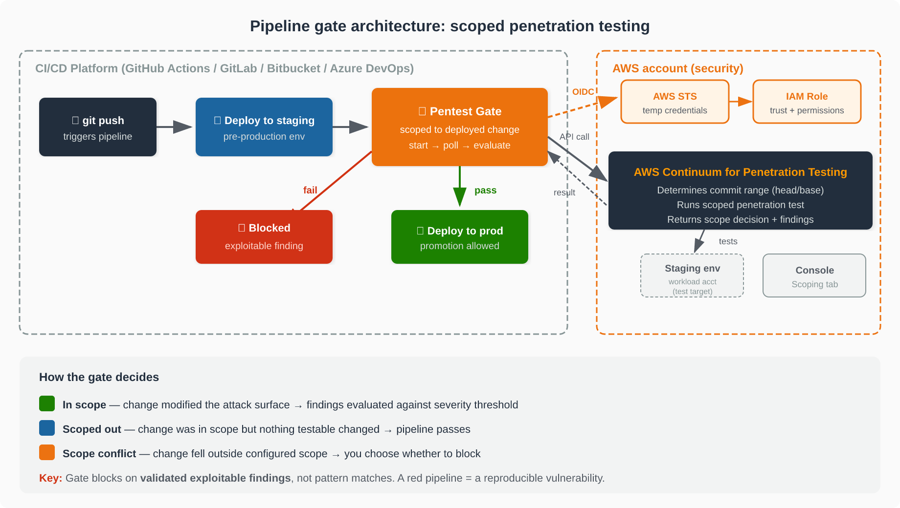
The following diagram shows the end-to-end flow. Your CI/CD pipeline deploys to staging, then the pentest gate step authenticates to your AWS account through OpenID Connect (OIDC) and calls Continuum for penetration testing, which runs the scoped test against the staging environment. The gate waits for the result, reports the outcome back to your pipeline, and conditionally blocks promotion to production. All testing runs server-side in your AWS account, so no penetration testing logic runs on your CI/CD runner.
Figure 1: Pipeline gate architecture: Your CI/CD pipeline deploys to staging, the pentest gate authenticates via OIDC and calls Continuum for penetration testing, which returns a scope decision that gates promotion to production.
Why scoping to the change matters
What makes the gate practical to run on every deploy is that it scopes each test to the change you just deployed. Continuum for penetration testing determines the commit range—the head is the commit being gated, and the base is the previous commit the gate already cleared—and tests only what changed. Testing the change instead of the whole application is what keeps a per-deploy penetration test fast and cheap enough to belong in a pipeline rather than on a quarterly calendar.
Each run returns one of three scope decisions: in scope (the change modified the attack surface—findings are evaluated against your threshold), scoped out (the change was within scope but nothing security-relevant changed—the pipeline passes), or scope conflict (the change fell outside the configured scope and was not tested—you choose whether that blocks). The Continuum for penetration testing console records the decision and the commit range on the Scoping tab of each run. When a gate blocks, you can see exactly why. For the full mechanics of how the commit range is computed and validated, see How the pipeline integration scopes the test.
Because the gate blocks on findings that Continuum for penetration testing validated as exploitable rather than on pattern matches, a red pipeline carries a clear meaning: a reproducible vulnerability in the change, waiting to be fixed before promotion.
Setting up the gate
The gate takes three steps to set up: configure a penetration test, create an AWS Identity and Access Management (IAM) role that your pipeline can assume, and add the gate step to your pipeline.
Before you start, you need an AWS account with permission to create both an IAM OIDC identity provider and an IAM role, and a staging environment the penetration test can reach.
Step 1: Configure the penetration test
Complete the one-time setup described in Before you start: verify your target domain, create a penetration test in your Agent Space, enable CI/CD mode, and connect your repository. Note the Agent Space ID (as-…) and penetration test ID (pt-…), because you pass both to the gate step in Step 3. The pipeline tests whatever this penetration test is configured to test, so its target and scope set what the gate covers.
Step 2: Create the IAM role
Authentication uses OIDC federation rather than stored keys. Your CI/CD provider issues a short-lived token identifying the pipeline, and AWS Security Token Service (AWS STS) exchanges it for temporary credentials when the pipeline assumes an IAM role you create. There are no long-lived AWS access keys to store as CI/CD variables, which removes the credential most often leaked from a pipeline.
The security of the gate rests on two policies: the IAM role’s trust policy (which pipelines can assume the role) and its permissions policy (what the pipeline can do once the role is assumed). For the exact policy JSON, the provider-specific OIDC URLs and audience values, and the sub claim format for each CI/CD platform, follow the reference in Scope the trust policy to your pipeline and Grant least-privilege permissions.
The following judgment calls help you decide how to scope these policies.
How tightly to scope the trust policy is the first decision. Pinning the sub claim to a single branch (for example, main) is the right default when a branch is the only one that deploys through this pipeline. If several branches or environments legitimately run the gate, scope to the environment instead of the branch where your provider’s claim supports it—and remember that not every provider carries a branch in the claim at all. On Bitbucket, the repository (and optionally a deployment environment) is as tight as it gets. Start as narrow as your deployment reality allows and widen only when a real branch or environment needs it. Note that GitHub repositories created or renamed on or after July 15, 2026 emit an immutable sub claim with numeric IDs—confirm the exact sub your pipeline emits before you write the policy.
Step 3: Add the gate step to your pipeline
The step is the same idea on every provider—the syntax differs. Pin the integration to an immutable version (a release tag, commit SHA, or pinned component version) so an upstream change can’t alter what runs in your pipeline. For the full settings reference and defaults table, see Defaults the integration ships with.
Before relying on the gate, run it once in dry-run mode. A dry run checks authentication, the Region, and that your repository resolves—without starting a scoped penetration test job. If validation fails, the step fails regardless of your error-handling settings, so a misconfiguration surfaces immediately.
A worked example: GitHub Actions
The following workflow shows the three-job topology that makes the gate work: deploy deploys to staging, security-pentest runs the gate, and deploy-prod promotes to production. Because deploy-prod declares needs: [security-pentest], GitHub skips production whenever the gate fails.
Note: The tutorials use an application with a deliberate SQL injection so the gate has a real finding to block on. Deploy it only to an isolated, non-production environment and remove it when you finish.
Replace the account ID, role name, Region, and the as-/pt- identifiers with your own values.
Two things in this example deserve attention. First, the contents: write permission lets the gate advance the baseline marker it keeps as a ref in your repository—without write access, every run would test a wider range than intended. Second, the role-duration-seconds: 7200 on the credential step must outlast the penetration test; AWS STS rejects a request for more than the role allows rather than reducing it, so set the role’s maximum session duration to at least (timeout + 10) x 60 seconds. A credential that expires partway through makes an otherwise-healthy run fail as though the service were at fault and leaves the cleanup unable to stop the abandoned, still-running job.
The full step-by-step tutorials for all four providers are linked at the end of this post.
Rolling out the gate: from report-only to blocking
The single most important detail before you roll this out.
Three independent settings decide whether the step fails, and each covers a different outcome: severity-threshold (what happens to findings), on-scope-conflict (what happens when the change wasn’t tested), and fail-on-infrastructure-error (what happens when the job couldn’t run). They are independent—relaxing one does not affect the others.
Most teams introduce the gate in report-only mode first—set threshold to NONE so the test runs and publishes findings without blocking anyone’s pipeline. Watch what it finds for a release or two, then tighten the threshold to HIGH. This staged rollout is sound, with one critical caveat:
A run that passes—including a report-only run—advances the baseline. The commits in that run’s range are then recorded as cleared and will not be re-tested when you later tighten the threshold. If you run report-only for a month and then switch to HIGH, the gate only assesses commits after the last report-only run—it does not go back and recheck what it already reported on.
This is by design: relaxing a setting is you accepting the outcome it allows. But if you want a stricter setting to reassess a range an earlier run cleared, override the head and base commit SHAs by settingbase-commit-shaandhead-commit-sha. Where the marker lives differs by provider; see What advances the baseline, and why that matters for the full matrix.
One default also deserves attention: fail-on-infrastructure-error ships as false (fail-open). For pipelines where promotion requires security sign-off, set it to true from the start.
GitLab: your committed settings are defaults, not a contract
On GitLab CI/CD, a pipeline variable overrides the value a job sets in its own variables: block. That means anyone who can run a pipeline could supply a variable that lowers the threshold, turns on dry-run, or relaxes error handling—and the gate does what the variable says, not what your .gitlab-ci.yml says. Restrict who may override variables in your project’s CI/CD settings before you rely on the gate to hold a release.
Protecting credentials on the runner
The temporary credentials and OIDC token are sensitive for the duration of the step. Three practices matter:
Keep debug and verbose tracing off for steps that handle credentials—shell-trace modes (for example, GitLab CI’s CI_DEBUG_TRACE) echo command arguments to the job log in plaintext.
Don’t persist source control credentials in the workspace—set persist-credentials: false on the checkout step so a token isn’t written to the runner’s .git configuration where a later step could read it.
Don’t expose the token to untrusted steps—grant OIDC-token permission only to the jobs that need it, and don’t run untrusted code (such as a fork build) in a job that can read the token.
Taking this to production and multiple accounts
The example uses one account for clarity. In practice, your staging and production environments are often separate AWS accounts. The pattern extends cleanly:
Create the pentest-gate IAM role in the account where the penetration test and Agent Space live—the security account. Your pipeline assumes that role via OIDC regardless of which workload account it deploys to, so you keep one well-scoped gate role rather than a copy or a set of long-lived keys in every account.
Run the gate against each pre-production environment you promote through, and gate promotion to the next stage on its result. Because the baseline advances only on a passing gate, coverage stays continuous across deploys.
Set fail-on-infrastructure-error to true and restrict who can override pipeline variables once the gate is holding real releases.
Pin the integration version so upstream changes are reviewed before they run.
For broader guidance of AWS Security Agent—testing against non-production environments, validating AI-generated findings, and IAM—see Security best practices for AWS Continuum.
Cleanup
If you followed one of the provider tutorials to try the gate, complete its Clean up section to remove everything it had you create: the sample application’s staging environment, the IAM role and OIDC identity provider, and—if you created one specifically for the walkthrough—the penetration test (and dedicated Agent Spaces) in the Continuum for penetration testing console. Removing them avoids ongoing charges and takes the intentionally vulnerable sample application offline.
Conclusion
Scoping penetration tests to the deployed change is what makes them practical as a per-deploy gate rather than a quarterly exercise. The key decisions you now have are:
How strict: Start report-only (NONE), but know the baseline advances—delete the marker when you tighten.
How to fail: Set fail-on-infrastructure-error to true for anything that requires security sign-off.
How to scope trust: Pin the sub claim as narrowly as your deployment reality allows.
Where to put the role: One role in a security account, assumed from workloads pipeline via OIDC.
To build the gate end to end on your platform, follow the worked tutorial for your provider:
The motivation for building the Netflix Foundation Model for personalization was laid out in this previous blog post. The Netflix homepage is powered by several specialized models and it requires significant time and resources to maintain and continue innovating on these individual models. Therefore, we decided to centralize member preference learning and have one powerful model learned from comprehensive user interaction histories and content data at a large scale and have this model distribute its learnings to other models.
The previous two blog posts(1, 2) focus on the development of the Foundation Model and here we talk about how we integrate the Foundation Model into various applications. We found that there is extensive literature focused on the training and inference of large-scale transformer-based models. However, there remains a significant gap in practical guidance and research on how to effectively and efficiently integrate large models into existing production systems. At Netflix, we experimented with 3 distinct integration approaches — embeddings, subgraph and fine-tuning. The motivation for trying different approaches stems from varying application needs. Specifically, different teams have different latency requirements, tech stack constraints and different appetites for leveraging the full power of a large foundation model.
In this blog, we go over the 3 approaches we experimented with and which are now used in production for different use cases. Each integration approach has its own set of motivations, tradeoffs, complexities and learnings. The following sections go into the details of each of these integration approaches.
Embeddings from Foundation model
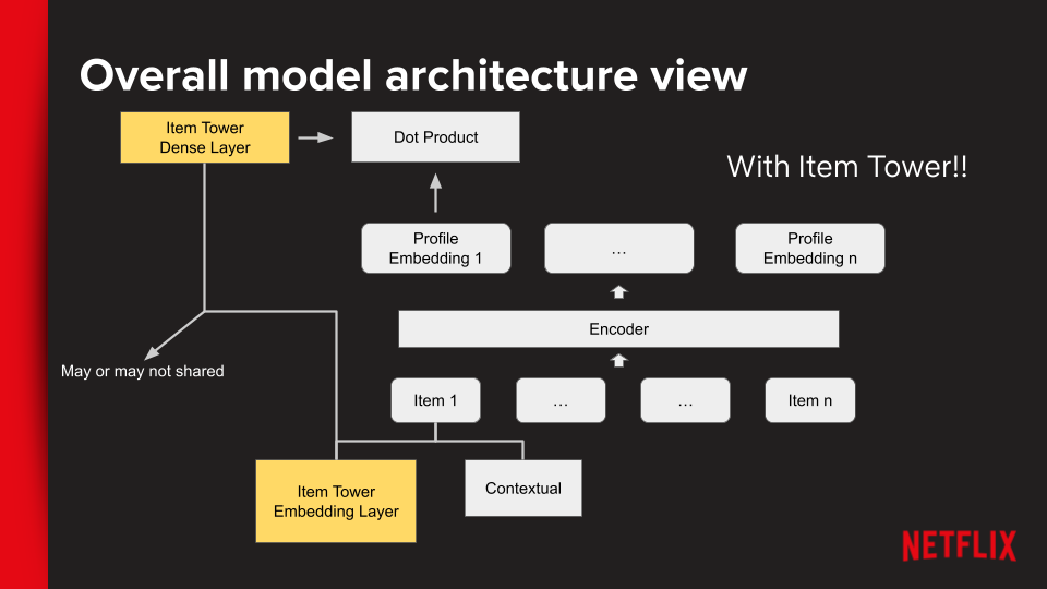
Transformer style foundation models naturally lend themselves to generating comprehensive user profile and item representations. Our approach for generating embeddings includes getting the hidden state of the last user event as the profile embedding and weights from the item tower as item embeddings.
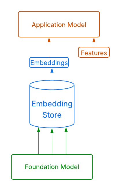
Netflix has an elaborate set up for refreshing the embeddings every day. First, the Foundation Model is pre-trained from scratch every month. Then, the monthly pre-trained model is fine-tuned everyday based on the latest data. The daily fine-tuning also expands the entity id space to include the newly launching titles. After the daily fine-tuned model is ready, we run batch inference to refresh the profile and item embeddings and publish them to the Embedding Store.
An important part of this setup is the embedding stabilization technique (paper). When the pretraining job retrains the model from scratch, the embedding spaces between different runs are completely different due to the random initialization in the model. In addition, the embeddings start to drift when the daily job fine-tunes on the latest data, despite the daily fine-tuning job warm-starting from the previous day’s model. Therefore, it is important to map the embeddings generated everyday into the same embedding space, so that downstream models can consume pre-computed embeddings as features.
This embedding approach relies heavily on the Embedding Store, which is a feature store specializing in embeddings built by the platform team at Netflix. The embedding store makes producing and consuming embeddings easy by taking care of versioning and timestamping the embeddings. The Embedding Store also provides various interfaces to access the embeddings offline and online.
Embedding Store integration
This approach is often the initial and most straightforward way for applications to interact with the Foundation Model. Embeddings can serve as powerful features for other models or for candidate generation, helping to retrieve appealing titles for a user or facilitate title-to-title recommendations. Integrating embeddings as features into existing pipelines is generally well-supported and offers a low barrier to entry. Compared to other integration approaches, using embeddings from the Embedding Store is expected to have a relatively smaller impact on training and inference costs.
However, this approach also has some cons. The time gap between embedding computation and downstream model inference can lead to staleness, impacting the freshness of recommendations. This may prevent applications from fully unlocking the benefit of the Foundation Model, especially for use cases requiring real-time adaptability.
Overall, the default starting point for leveraging the Foundation Model is through its profile and item embeddings via the Embedding Store, provided that the embeddings’ freshness and stability meet application-specific needs. While embeddings may not leverage the full power of the Foundation Model, they offer a good initial step.
Our biggest learning from working on this approach is that embeddings are a low cost and high leverage way of using the Foundation Model. A resilient embedding generation framework and embedding store are essential for updating the embeddings daily and serving them to application models. We found this infrastructure to be so valuable that we stepped up our investment here to build a near-realtime embedding generation framework. This new framework also enables us to update the embeddings based on user actions during the session, making the embeddings and our downstream models more adaptive. Although the near-real time framework cannot be used for very large models, it represents an important direction for addressing embedding staleness and adaptiveness of recommendations.
Foundation Model as a Subgraph
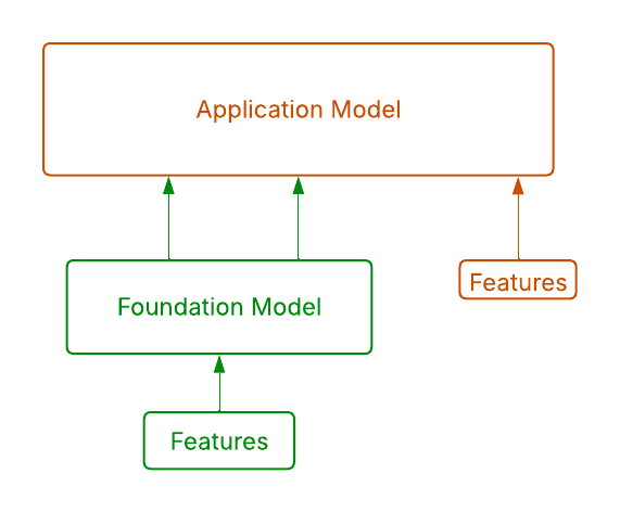
This approach involves using the Foundation Model as an input to the downstream model i.e. the Foundation Model decoder stack is a subgraph of the application model’s full model graph and hence the name “subgraph integration”. The Foundation Model subgraph processes raw user interaction sequences and outputs representations that are then fed into the downstream model graph.
Foundation Model Subgraph integration
Applications can fine-tune the Foundation Model subgraph as part of their own training process, potentially leading to better performance than just using static embeddings. In this approach, there is no time gap or staleness between the Foundation Model inference and the application model’s inference, ensuring that the most up-to-date learnings are used. This approach also allows applications to leverage specific layers from the Foundation Model that may not be exposed through the Embedding Store, uncovering more application-specific value.
However, the subgraph approach comes with some complexities and trade-offs. To use the Foundation Model as a subgraph, application models need to generate all the features necessary for the subgraph as part of their feature generation process. This can add time, compute and complexity to their feature gen jobs. Merging the Foundation Model as a subgraph also increases the application model size and inference time. To alleviate some of these complexities, the Foundation Model team provides some reusable code and jobs that make the feature generation more compute efficient. To optimize the inference performance, we split the subgraph and ensure it only runs once per profile per request and is shared by all items in the request.
Overall, the subgraph approach allows for a deeper integration and enables the applications to harness the full power of the Foundation Model. But it can also make the application’s training code more complex, requiring a trade-off between metric improvement, compute cost, and time. Therefore, we would reserve this approach for high impact use cases where the increase in metric wins compensate for the cost and complexity.
Fine-tuning Foundation Model and use directly
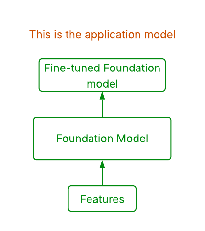
This approach is similar to fine-tuning LLMs with domain specific data. In the previous blog post, we described how the Foundation Model is trained on a next-token prediction objective, with the tokens being different user interactions. Different interactions are of different importance to various surfaces on the Netflix website. For example, for the ‘Trending now’ row, recent interactions on trending titles might be more important than old interactions. Hence, the Foundation Model can be fine-tuned on more product specific data and then the fine-tuned model can be used to directly power the product. During fine-tuning, application teams can choose to do full parameter fine-tuning or freeze some layers. They can also choose to add a different output head with a different objective. We built a fine-tuning framework to make it easy for application teams to develop their own custom fine-tuned versions of the Foundation Model.
Fine-tuned Foundation Model Integration
This approach offers the ability to adapt the Foundation Model to application’s specific data and objectives, making it optimized for their use case. A side benefit of this integration approach is that it provides a de facto baseline for new models/applications. Instead of coming up with a new model stack and spending months on feature engineering, new applications can directly utilize fine-tuned foundation models. However, this approach can lead to more models and pipelines to maintain across the organization.The latency and Service Level Agreements (SLAs) of the fine-tuned model must be carefully optimized for the specific application use case.
Conclusion
We are continuing to innovate on these integration approaches over time. For example, the Machine Learning Platform team is working on near-real time embedding inference capabilities to address the staleness issues with the embedding approach. We are also working on a smaller distilled version of the Foundation Model to reduce the inference latency of the subgraph approach. We also provide a fine-tuning framework to make it easy to fine-tune and leverage the Foundation Model. We also continue to refine and standardize the APIs used in these approaches to make it easy for application teams to use them. Overall, these three integration patterns provide a comprehensive framework for how Netflix applications can interact with and extract value from the Foundation Model.
Acknowledgements
We thank our stunning colleagues in the Foundation Model team for developing and continuing to innovate on the Foundation Model. We thank our colleagues in the AIMS applications teams for driving the integrations and their valuable feedback and discussions. We also thank our Machine Learning Platform team for building and supporting the infra components to get these approaches up and running in production.
Our Netflix journey from data to dashboards, particularly within the space of the experimentation platform, always presented a unique set of challenges. This blog post aims to illuminate these hurdles and explain how an innovative open-source metric platform became instrumental in overcoming some of them. We’ll showcase the critical role that DataJunction played in streamlining our data workflows and enhancing our ability to derive meaningful insights from our vast datasets.
Metrics are the foundation of data-driven decision-making, but at many organizations, they are scattered, inconsistently defined, and difficult to discover or trust. At Netflix, this challenge first became apparent in our experimentation platform, where reliable metrics are essential for interpreting test results. But the complexity of the original tooling made it very difficult to understand and introspect these metrics both in terms of their definitions as well as their values.
Initial Problem
Scattered metric definitions, redundant datasets, and pipelines are often a natural effect of a fast-moving company with a large and powerful analytical workforce. This is a common problem in big data-driven firms, and it is not easy to solve across multiple departments, which are often governed by somewhat different rules and regulations. An easy-to-use, well-governed, and centralized semantic layer can help with these issues. Our initial problem was most evident in our Experimentation Platform team, where the previous system required:
extensive business knowledge
familiarity with experimentation conventions
and complex engineering practices
This led to metric authoring processes that would take weeks, which was a prohibitive requirement for Data Scientists and Analytics Engineers who wanted to onboard new metrics to the Experimentation Platform.
Enter DataJunction
To address this problem and to set ourselves on the path to a successful semantic layer solution in the future, we looked at several candidates. Among other solutions we evaluated Mando (an internal framework), Minerva (an open source semantic layer from AirBnB), and DataJunction (another open source solution, “DJ” for short). All of them had some strength, but DJ offered one thing that the others did not at the time: a solid SQL parsing and SQL generation engine. At the time of the POC, DJ was also the only open-source solution that stored all its definitions in a connected graph, similar to how relational databases store metadata on their views and queries. Easy “SQL wrangling” with rich metadata was the main feature that convinced us to try it for our immediate use case.
DataJunction originated from a similar internal Facebook project created (around 2015) by the data science and infrastructure (DSI) team, mainly as an answer to the need for metrics portability. During several iterations of the Deltoid project — which was the main experimentation platform at Facebook at the time — users were required to rebuild and repopulate their metrics when they wanted to move to the next version of Deltoid. But after implementing DJ and abstracting all metric definitions the team offered seamless migrations by separating the concerns between the metrics and the stats computation platform. That project was subsequently renamed to MDF (Metrics and Dimensions Factory) and promoted as a generic semantic layer used widely by various departments. In 2021, one of the Facebook engineers (Beto Dealmeida), started the DJ Github project and built out some basic functionality. Then together with some folks at Netflix expanded the scope further, and soon after that the project was introduced at Netflix. Following that introduction, three Netflix engineers (authors of this blog) together with a couple of external contributors, most notably Nick Ouellet, have been building out the remaining features of the platform.
Architecture Decisions
A critical design constraint for building DJ at Netflix was resource scarcity. We refused to compromise on product quality, choosing instead to limit the feature set. Although DJ was clearly capable of addressing many simultaneous problems across diverse use cases, our lack of adequate resources and official support meant we developed it as a side project for over two years. Our hope was that demonstrating its value would eventually secure management attention.
API First, UI and Other Interfaces Later
A metrics platform doesn’t need a flashy front-end to deliver value — its core is the semantic layer, which stores a consistent set of dimensions and metrics and serves this information through a rich API service. You can see below how we structured the main components of DataJunction in the Netflix implementation. Our DJ services (in the middle) interact with the underlying data (on the left) and supply our access layer with the business definitions in the form of SQL w/ metadata or directly with data depending on the client request.
Consistent Graph First, Other Features Later
A complete semantic layer system can seem like an octopus, with its tentacles reaching out into many functional areas and can expand from a basic semantic metadata stored for some datasets to full dashboard functionality. Let’s call out some of them:
semantic metadata authoring and management and monitoring
metric and dimension query / definition generation
metric and dimension data generation (requires a query engine)
data visualization and data tracking
performance optimization (aka caching or materialization)
integration layer with other tools and
any / all the above functionality served as: UI, API, client libraries, MCP servers and more.
Of course it is extremely hard to provide the best in class functionality across all these layers, so with our small “unofficial” team we decided to focus on the most important piece: solid semantic layer engine (and API) with the ability to parse SQL as the input to the graph and generate SQL as the serving layer. That is the core of the system and everything else can be added later with less effort and w/o the need to rebuild the core.
Cube as The Perfect Consumption Protocol
Analytical multi-dimensional cubes have been a fundamental concept for decades, with their representation integrated across various data processing and analysis platforms. While definitions and features may vary between tools, they all serve the common purpose of encapsulating, or abstracting, a subset of semantic objects.
In DataJunction, we adopted cubes as first-class features for two main reasons: their familiarity to users and their suitability as a serving interface. They efficiently deliver both the semantic definitions (of metrics and dimensions) and fast data access. See an example of data “flow” graph (dotted lines) and dimensional relationships graph (solid lines) below.
We simplified the creation of basic cubes, allowing them to easily aggregate arbitrary collections of shared metrics and dimensions. Furthermore, accessing, managing, and visualizing these cubes is straightforward for any client integrating with DJ. Custom integrations, such as for Netflix’s internal fast Druid data analysis tool (Data Explorer → see below), became trivial to build, and we also made it easy to materialize these cubes directly in our Druid clusters.
One of DJ’s most powerful client integrations is the ability to link any DJ-originating metric definition back to the DJ ecosystem. This creates a valuable feedback loop: troubleshooting and introspecting business dashboards becomes simple if they display DJ-defined metrics that include links back to the definition source. This link then makes inspecting and running ad-hoc analysis, by modifying existing metrics, a trivial process. This integration is not only possible with our inhouse tools, but also with other well known open-source products, like Superset.
Experimentation at Netflix
Metrics are the backbone of experimentation. They translate data into signals that tell us whether a change is meaningful, safe, and worth scaling. Without trustworthy metrics and dimensions, experiments risk becoming inconclusive or misleading, so a robust metrics layer becomes crucial for data-driven decisions.
At Netflix, the original metrics layer integrated into the experimentation platform was overly complicated. Creating new metrics not only required tribal knowledge of experimentation data artifacts, but also familiarity with complex engineering workflows. This unnecessary friction meant that onboarding a single new metric could take weeks, slowing adoption of new metrics and hindering experimentation.
This is where DataJunction comes in: it provides a central hub for defining metrics and dimensions that can easily be shared and explored via the semantic graph. It also provides flexible, user-friendly interfaces (including a UI, API, and various clients), making it easy for users to author and manage their metrics and other semantic models.
Conclusions
With experimentation domain well supported by DataJunction, we would like to take on next steps to unifying of the general analytics at Netflix and to make it easier for Netflix users to both:
find and use metric definitions across verticals (defined in DJ)
easily access, modify and experiment with new metrics across Netflix data stack
That will require building out strong integrations between DJ and other tools, but that has been underway and it is one of the most enjoyable parts of this project, where most of the feature exists and we are simply enabling existing systems to exchange information in a structured and reliable way. With a system like DataJunction our internal LLMs can deliver accountable information about the business metrics as well as explanation of how they are defined and used across Netflix.
By Kevin Zielnicki, Guy Aridor, Aurélien Bibaut, Allen Tran, Winston Chou, and Nathan Kallus
Introduction
Personalization is everywhere on the internet. It shapes the products we discover, the stories we read, the music we hear, and the movies and TV shows we watch. At Netflix, personalization has been central to the member experience for decades — from the Netflix Prize to our modern recommender system that helps members navigate a large and constantly changing catalog.
But personalization is not only an algorithmic problem, it is also a measurement problem. How do we know how much value personalization creates? More precisely, how do we separate the appeal of a title from the value created by recommending that title to the right member at the right time?
In a new article in the International Journal of Industrial Organization — which we are also presenting at this year’s ACM Conference on Economics & Computation (EC ‘26) — we develop a model of member behavior, title choice, and personalized recommendations. The model lets us estimate how recommendations affect both whether members choose to watch and, if so, which titles they choose. In this post, we summarize our approach and main findings.
The Measurement Challenge
A natural first attempt at valuing recommendations is to ask: what share of viewing comes from titles that were recommended? This is an intuitive metric, but it fails to answer the causal question at hand.
The problem is that recommendations are not randomly assigned. A title appears on a member’s homepage precisely because the recommender system predicts that the member might want to watch it. If a member watches that title, was it because the recommendation caused the member to watch it? Or would she have watched it anyway because of her underlying preference for that kind of title? This is the core measurement challenge: recommendations are targeted to demand, so viewing a recommended title combines the effect of personalization with the member’s underlying preferences.
One way to solve this would be to run a large experiment that replaces Netflix’s personalized experience with an unpersonalized one. That would create clean variation — but it would also be a poor member experience. Personalization is a central part of how members locate valuable titles in a large catalog, so turning it off broadly is not an acceptable measurement strategy.
Instead, we take a hybrid approach. We build a behavioral model that separates members’ underlying preferences from the incremental effect of recommendations. The model uses the natural variation in the recommendation system, for example due to algorithmic exploration, to estimate how recommendations affect choice. Then, to validate the model predictions about title substitutability, we use small-scale A/B tests that “nudge” the salience of a handful of titles exogenously, generating ground-truth substitution patterns for a subset of titles. This lets us combine the scale and richness of modeling with the credibility of experimental evidence.
A Model of Member Choice
To measure the value of personalization, we need a model of what members would watch under different recommendation systems. Our model treats Netflix viewing as a day-by-day choice process. On each day, a member chooses among the titles available in the catalog, or she chooses not to watch anything. This gives us a concrete target to estimate: the probability that a member watches each title on a given day, as a function of their preferences, their viewing history, and the recommendations they see.
A simple version of this model would be too restrictive. It might assume, for example, that removing one title from the catalog shifts viewing toward all other titles in roughly proportional ways. But that isn’t how member choice works. If a member is considering a romantic comedy, the closest substitutes are likely other romantic comedies, not every title on Netflix equally. For similar reasons, two members may react very differently to the same recommendation.
To capture this complexity, we use a low-rank choice model. The model learns a representation of each title and a corresponding representation of each member’s current preferences. These representations are not limited to manually specified features like genre, cast, or language. Instead, they are learned from viewing behavior itself, allowing the model to capture nuanced similarities between titles that may be difficult to describe with coarse features, such as genre or release date, alone.
Our Model Attributes Choices to Dynamic Member-Title Affinity and the Effect of Recommendations
Member preferences are dynamic. What someone wants to watch today depends on what they have watched recently. A member who just finished a crime thriller may be in a different preference state than the same member after watching a stand-up special or a kids’ movie. Rather than estimate a fixed preference vector for each member, the model summarizes each member’s past viewing history into a current preference state. This lets us capture heterogeneous and time-varying tastes while also scaling to millions of members.
Our Model Architecture Allows Us to Scale to Millions of Members Efficiently
The key component for our purposes is that the model explicitly parameterizes the effect of recommendations. When a title is recommended, the model gives it an additional recommendation effect, or “bonus,” that increases its probability of being chosen. This bonus is a reduced-form way to capture two related mechanisms. First, recommendations can create awareness by helping members discover titles they may not have known about. Second, recommendations can provide information by signaling that a title is likely to be a good match.
Once estimated, the model becomes an engine for predicting counterfactuals. We can ask what would happen if a title were not recommended, if a different set of titles were recommended, or if the current recommender system were replaced with simpler alternatives. Because the model separately represents member preferences, title appeal, and recommendation effects, it lets us estimate not only how recommendations affect total viewing, but also how they change which titles are watched.
The model is only useful, however, if it captures real substitution patterns. The next step is therefore validation: comparing the model’s predictions to randomized experiments that directly perturb, on a small scale, the visibility that each title receives.
Validating the Model with Randomized Experiments
The model relies on an important assumption. After conditioning on the member, title, and state information available to the recommender system, we treat the remaining variation in whether a title is recommended as if it were randomly assigned. In our setting, this assumption is reasonable: we observe all of the information available to the recommender system, so we should be able to model its behavior accurately. But it is still an assumption. A useful model should not only fit historical viewing patterns; it should also predict what happens when recommendations change for external reasons.
Thus, to validate the model, we used randomized experiments that introduce variation in title visibility exogenously. These experiments mirror the kinds of variation that occur routinely when recommendation algorithms are updated: some titles receive more impressions, while others receive fewer. The key difference is that, in the validation experiment, this variation was prespecified so that we could estimate clean experimental benchmarks.
Specifically, we randomly assigned members to treatment arms that slightly nudged recommendations towards and away from different categories of titles. This let us measure diversion ratios: when a set of titles becomes less visible, how much viewing shifts to other titles, and how much shifts out of Netflix viewing altogether?
We then asked whether the model could reproduce those experimentally measured substitution patterns. We estimated the model on the control group, simulated the same recommendation changes, and compared the model-implied diversion ratios to the experimental ones. The agreement was strong: the model’s predicted diversion ratios had a correlation of 0.86 with the experimental estimates and an R-squared of 0.73.
Our Model Predicts Out-of-Sample Experimental Diversion Ratios Well
This validation gives us confidence that the model captures counterfactual substitution patterns accurately. Subsequently, we ask what would happen under more dramatic changes, such as different recommender systems.
Counterfactuals: Aggregate Consumption and Diversity
With a validated model in hand, we can move from measurement to counterfactuals. Instead of asking only what happened under the current Netflix experience, we can ask what would have happened if members had seen recommendations generated by a different system.
We compare the current recommender system to three baselines:
The first is random recommendations: every member receives titles selected uniformly at random from the catalog. This is not intended as a realistic product experience, but it helps isolate the value of having recommendations that are relevant.
The second is popularity-based recommendations: every member receives broadly popular titles. This is a natural non-personalized benchmark.
The third is a basic matrix factorization model, a classic personalized recommendation approach and a useful baseline for older generations of recommender systems.
In each counterfactual, we replace the recommended titles while keeping the rest of the choice environment fixed. This lets us estimate how much viewing would change if the recommendation policy changed, holding constant the catalog, members, and model of member choice.
The results show that the current recommender system generates substantially more engagement than each benchmark. Relative to the current system, random recommendations reduce engagement by 16%, popularity-based recommendations reduce engagement by 12%, and matrix factorization reduces engagement by 4%. These are large differences at Netflix scale. Even the comparison to matrix factorization — a personalized baseline — suggests that continued improvements in personalization translate into meaningful gains in how effectively members find titles they want to watch.
Personalized Recommendations Increase Engagement and its Diversity
Engagement is only part of the story. A recommender system could increase viewing while concentrating attention on a narrow set of already-popular titles. That would be a worse experience for members whose tastes are not well represented by those titles, and it would make poorer use of a broad catalog.
We therefore also examine consumption diversity: how broadly viewing is distributed across titles. The current system performs well on this dimension too. Popularity-based and matrix-factorization recommendations both substantially increase concentration, meaning that fewer titles receive meaningful viewership. Random recommendations produce slightly more diversity, as expected, but at a large cost to engagement.
Taken together, these counterfactuals show that the value of personalization is not just that members watch more. It is also that members are matched to a broader set of titles. The current recommender system increases engagement while preserving a wide distribution of viewing, reflecting the diversity of member tastes across the Netflix catalog.
Decomposing the Impact on Titles
The aggregate counterfactuals show that personalization increases engagement while maintaining broad consumption across the catalog. We can also use the model to ask a more granular question: why does a recommended title get watched?
There are three conceptually distinct channels:
The first is exposure: simply showing a title to a member can increase the probability that the member watches it. This captures the basic value of surfacing a title that may otherwise have been hard to find.
The second is selection: recommended titles are shown to members who already have a relatively high baseline probability of watching them. This channel doesn’t lead to incremental engagement, but it can smooth the discovery experience and help users feel that the recommender system understands their preferences.
The third is targeting: the recommender system may identify members for whom the recommendation itself is especially effective, meaning members who are much more likely to watch the title when it is recommended than when it is not.
The distinction matters because not all recommendation-driven viewing should be interpreted the same way. If recommendations worked only through exposure, then any reasonably visible surface could generate much of the same value. If they worked mostly through selection, then recommendations would mainly be finding members who were already likely to watch a title. Targeting is different: it captures whether the system is placing titles in front of members for whom the recommendation changes the decision.
Decomposing the Impact of Recommendations into Selection, Exposure, and Targeting
Our model lets us estimate these channels title by title. For each title, we can compare the predicted probability that a targeted member watches it when recommended to the probability that an average member watches it when not recommended. We then decompose that difference into selection, exposure, and targeting.
We first show that exposure is meaningful: showing a title to an average member roughly triples its consumption probability relative to the baseline. Exposure is not the main driver of differences in consumption, as mechanical exposure explains only about 7% of the gap under the current recommender system, while selection and targeting account for the vast majority of the difference and the targeting effect is nearly seven times larger than the exposure effect.
This pattern is especially informative when compared with simpler recommendation systems. Random recommendations are dominated by exposure because they do not personalize: differences in consumption mostly reflect differences in what titles are shown. Matrix factorization changes this by making recommendations personal, reducing the role of exposure and leaving exposure, selection, and targeting to contribute nearly evenly to consumption differences. The current recommender system goes further: its gains come less from mechanical exposure, but more from targeting the right titles to the right viewers.
Targeting is also not uniform across the catalog. It is strongest for mid-popularity titles: titles with enough potential audience to be broadly relevant, but not so much mass appeal that everyone already knows about them. Very popular titles need less help from targeting, while very niche titles may have too small an audience to target effectively. The largest gains come from the middle of the catalog, where personalization helps connect specific titles with specific member tastes.
Personalized Recommendations Give the Strongest Boost to Medium-Popularity Titles
Conclusion
Personalized recommendations are valuable because they help members navigate a large catalog and find titles they want to watch. They are also valuable to Netflix because they make the service more useful, more engaging, and better able to serve a wide range of tastes.
But measuring that value is not straightforward. Recommendations are targeted by design, so we cannot simply compare recommended and non-recommended viewing. At the same time, turning off personalization at scale would create a worse member experience.
Our approach combines a large-scale model of member choice with true experimental validation. The model lets us separate underlying title preferences from the incremental effect of recommendations, and the experiments verify that the model captures real substitution patterns.
Using this framework, we find that personalization affects both how much members watch and which titles they watch. The value of recommendations comes not just from exposure, but from matching the right titles to the right members.
In an earlier post, we introduced the TimeSeries Abstraction, our high-throughput, low-latency platform designed to store and query temporal event data at scale. It has since become the operational backbone for Netflix’s largest datasets, which now span multiple petabytes.
However, managing such large datasets in hot storage, tuned for low-millisecond latency access, is not cheap. At Netflix, cost-efficiency is a continuous discipline rather than a temporary initiative. This post shares two solutions that significantly reduce storage costs by continuously moving older, less frequently accessed data into cheaper object storage:
We’ll start with the Kafka/Flink-based design, then describe how we evolved to a native Cassandra-based cold tier.
Challenges
As Netflix’s TimeSeries datasets have expanded, we’ve encountered several compounding challenges:
Growing retention demands: Users often push for increasing data retention to serve a broader range of use cases, which in turn increases the storage costs.
Escalating costs: Maintaining massive, dense clusters for infrequently accessed historical data is prohibitively expensive.
Sparse historical access: Most queries target recent events, but older data must remain readily available for occasional audits and investigations.
Operational strain: High storage density on hot nodes complicates scaling, deployment, and cluster stability.
Latency requirements: Even historical data sometimes requires sub-second query performance for internal tooling and analysis.
This creates a clear opportunity: keep the most recent data on fast storage and migrate older, rarely read data to cheaper storage while preserving a consistent API. Done well, this can meet user and operational needs while greatly reducing our infrastructure spend.
TimeSeries Abstraction
Before we dive into the cold storage solutions, here is a quick recap of how TimeSeries partitions its dataset into multiple tables, each covering a window of time we call Time Slices.
Time Slices and Immutable Windows
This enables several key optimizations, most notably allowing a table to become immutable once it crosses the write boundary, which lets us safely apply further optimizations. For more details, refer to our previous post.
This slice information is critical and is maintained in a dedicated metadata table:
Time Slice Metadata Storage
Creating new Time Slices and maintaining their metadata is a primary responsibility of the TimeSeries control plane. The TimeSeries data plane uses this information to correctly route the read and write traffic to the provisioned tables.
TimeSeries Data and Control Plane
With that background, let’s look at the different solutions we built for data tiering.
Solution 1: Streaming with Apache Kafka and Flink
Our first solution followed a familiar streaming pattern using Apache Kafka and Flink, where we streamed data to S3 in realtime while simultaneously persisting it to Cassandra.
Streaming with Apache Kafka and Flink
Getting Data Into S3 Efficiently
To optimize data streaming to S3, the system hash-partitions Time Series IDs into buckets. This partitions the stream and lets dedicated Flink tasks handle each bucket, ultimately batching and reducing the write throughput to S3. Flink workers batch events into Parquet files grouped by event time within the hour. These files are great for high-throughput streaming writes, but not for low-latency reads.
Enter the Compaction job.
Compaction Job to Optimize Reads
The compaction job runs daily and merges small Parquet files into a single, optimized daily Parquet file per namespace.
The job further optimizes the Parquet files in the following ways:
Small Row Groups: Creates small (4–8 MB) row groups to minimize lookup cost. We can then use the Parquet Java library to perform range reads of row groups from S3. This is intentionally well below Parquet’s recommended row group floor — smaller groups were better because our reads are dominated by point/range lookups rather than full scans.
Event Sorting: Sorts events within a row group by time, eliminating brute-force scans when querying for a time range.
Bloom Filters: Caches Bloom filters and file metadata in EVCache, allowing the TimeSeries query planner to efficiently skip unnecessary reads from S3.
Compacted and Sorted Parquet File Layout
Once the compaction job completes, all compacted files per partition are recorded in the TimeSeries control plane, and the hot storage slices can now be truncated!
On some of our largest datasets, this job typically takes about 12 hours, prioritizing lower compute costs over execution speed.
Compaction Burndown Per Day
Streaming Cold Tier Read
Once compacted files are optimized in cold storage, they are ready to be read. The TimeSeries data plane fans out a given query across both the hot and cold tiers and merges their result. The users still use the same query interface:
TimeSeries Tiered Storage Read Path
The Cold Tier Data Plane uses compaction metadata for aggressive planning and pruning, which dramatically reduces the S3 query fan-out. As a result, retrieving a full day of data requires at most three sequential S3 reads, even in the uncommon case where an ID spans two row groups. This yields a p50 latency of ~150 ms and a p99 latency of ~500 ms per read.
Cold Tier Read Latency in Seconds
At the time of writing, the streaming cold tier implementation was processing up to 1,250 reads per second from cold storage globally:
Cold Tier Read Requests Per Second
Why not stop here?
The streaming cold tier has delivered real savings, shrinking both Cassandra’s EBS footprint and the Cassandra backup footprint in S3. But the streaming infrastructure itself is expensive and adds moving pieces that widen the team’s on-call scope:
Additional Infrastructure and Operational Cost
We wanted to improve this further and asked ourselves:
Can we avoid streaming data into the object store and the associated data transfer costs?
Can we reduce the compute and operational overhead of new components?
That led to a more radical question: Can we read directly from existing Cassandra backups in S3?
Solution 2: Cassandra Cold Storage for Immutable Data
At Netflix, we back up Cassandra data into S3 at regular intervals for disaster recovery. The idea for tiering is simple:
Read directly from these S3 backups instead of paying a separate data transfer cost to S3.
Once TimeSeries marks a hot Time Slice as ready for cold storage, we can customize Cassandra to read directly from its backups, allowing us to delete the on-disk data copy. This would also incur minimal changes to the TimeSeries read path!
New TimeSeries Read Path
To make this viable in production, we had to answer a series of “How…?” questions.
How Can We Read the Backups Efficiently?
We introduced a new compaction strategy in Cassandra, which we call ReadOnlyCompactionStrategy (ROCS). Here is how it works:
Once a time slice crosses the user-configured cold-tier boundary, TimeSeries stops accepting writes for that time slice making it immutable. This immutability unlocks significant optimization opportunities:
SSTable overlap: Standard strategies (LCS, TWCS) often produce SSTables that overlap in the token space, and so a single partition key may exist across multiple files.
Read fan‑out: Because a read must touch every SSTable covering the key’s token range, this overlap turns a single point-read into multiple lookups, increasing latency across all tiers.
ROCS re-compacts all SSTables once, aligning them precisely with token ranges:
ROCS SSTable Boundaries
ROCS applies more broadly to all TimeSeries use cases, driving tail latency down on all storage tiers by reducing the SSTable fan-out during read operations:
Tail Latency Improvement in Reads after ROCS
Once the immutable Time Slices have been optimized, it is time to trigger backups.
How Would We Leverage Backups?
Cassandra backs up every node in the cluster, organizing each backup on S3 as a declarative manifest, along with the SSTables backing the keyspace’s tables:
Alongside the large Data.db file, backups include a compact set of index, metadata, and integrity files. This structure allows us to quickly locate, validate, and restore specific partitions or data ranges without scanning the entire dataset. Furthermore, since the manifest catalogs every S3 path, we can download most of these components directly to the Cassandra node (excluding the Data.db file) where they occupy negligible space. These local components enable efficient query planning before any data is read from S3.
How Would Cassandra Read From Backups?
Cassandra reads typically pull data from two sources: the Memtable, which holds recent unflushed writes, and flushed SSTables on durable storage. As of Cassandra 4.1, we can leverage pluggable Memtables to redirect reads from “cold” tables directly to the backup storage in S3.
-- create table for a given Time Slice
CREATE TABLE data_20260616_00_04 (
    ...
    ...,
    PRIMARY KEY ((time_series_id, time_bucket, event_bucket), event_time, event_id, key)
) WITH CLUSTERING ORDER BY (event_time DESC, event_id DESC, key DESC)
    ...
    AND compaction = ...
    AND compression = ...
    AND memtable = 'backupmemtable:timestamp=1781953200000' ← Custom memtable
    ...
The timestamp marks the point at which the backup is guaranteed to cover the full table, and the table is guaranteed to be immutable.
Opening a backup Memtable kicks off a state-machine initialization that pulls the index data from S3 onto the node once:
State Machine for Cassandra Backup Memtable Initialization
This process ensures all SSTable components are downloaded reliably through several resilience mechanisms:
Retries and backoff: All S3 operations and file-system cache writes use retries with exponential backoff.
Resource isolation: Initialization runs on a dedicated thread pool, isolated from normal Cassandra operations.
Partial download protection: If a downloaded component’s size doesn’t match the manifest, it is deleted and re-downloaded.
DDL change protection: A .timestamp file marks completed initialization and ties it to the backup timestamp. If the table’s backup timestamp changes, this file is removed and initialization restarts for the new timestamp.
Read protection: Memtable initialization is asynchronous; reads to an initializing memtable block for at most half the read RPC timeout.
Once initialization has pulled every SSTable component (except Data.db) from S3 onto the local disk, the Memtable is ready to serve reads. Here is what the read process looks like:
Reading from Cassandra Backup Memtables
To minimize latency, the system parallelizes S3 reads across requests, SSTables, and individual chunks. A shared cache deduplicates fetches and prefetches data, so chunks are ready before they are needed.
We further optimize cluster and table settings to reduce the number of S3 calls:
Larger compression chunks: Reduce S3 calls per partition by reading fewer, larger chunks (accepting some over-fetch on small reads).
The TimeSeries control plane automates the entire transition as slices cross the immutable boundary:
Automating Time Slice Lifecycle Transitions
Each slice can be in any lifecycle stage at any time without impacting system availability, and the system remains resilient to delayed backups or lagging compactions.
How Would Cassandra Handle The Additional Load?
Serving data from S3 is much more CPU-intensive than reading from local storage. A sudden spike in read requests can overwhelm the Cassandra cluster and affect the hot path, turning a cost-saving feature into a reliability risk.
To avoid this, cold reads can optionally run on a separate Cassandra cluster that points its backup Memtables at the hot cluster’s backups:
Isolated Cold Tier Cassandra Topology
The cold Cassandra cluster must match the original cluster in topology but need not match it in hardware! We can run the cold cluster on much smaller, cheaper, storage-light instances.
Real World Performance
Cassandra Cold Tier was rolled out to the most storage‑intensive TimeSeries Abstraction clusters. It currently stores over 15 PB of compressed data in Cassandra cold storage and has allowed us to cut attached storage significantly on all affected clusters:
Storage Reduction During Rollout: from 80% disk usage to 7%
At the same time, it serves thousands of reads per second from cold tier storage in any given region:
Cold Tier Read Requests Per Second
Cassandra Cold Tier improves p90 latency by ~30% over the previous cold storage implementation, thanks to more efficient S3 access patterns and smaller read sizes, while keeping p99 latency under ~500 ms. Cassandra already handles bursts of cold reads gracefully via its chunk cache, so this design preserves that same resilience for the S3-backed cold tier:
Cold Tier Read Latency: blue — p90 latency, brown — p99 latency; latency measured in seconds)
In Part 1 of this series, we shared how Netflix built the Ads Event pipeline and approached it as a system design problem: replacing fragmented pipelines with a centralized collection, enrichment, and a standard data contract. The result was Ads Event Publisher, the system that collects ad telemetry from client devices, enriches it with the context of the ad that was actually served, and publishes a single, unified stream of ad events to every downstream consumer: frequency capping, metrics, billing, measurement partners, and reporting. Any member viewing or account details that move through this pipeline end-to-end are encrypted and handled in accordance with Netflix’s strict privacy and security practices to safeguard member PII.
If ad serving is the “brain” and ad events are the “heartbeats” that feed it, then enrichment is what gives each heartbeat its meaning, turning a bare “[Somebody] watched an ad to completion” signal into “this campaign, this creative, at this price, for this break.” Part 1 described that enrichment step as a single box in the architecture. This post is about what was inside that box, and why we rebuilt it.
Part 1 ended with a look at what was on the horizon: ads on live streams, de-duplication, and richer data signals. A single project delivered all three by rebuilding the Ads Event Publisher around stateful stream processing. We replaced a database lookup with a real-time streaming join in Apache Flink, which let the system scale for Live, took a dependency off the critical path, and replaced the engine of a high-traffic pipeline without downtime.
Let’s dive in.
A quick recap: enrichment and the Metadata Registry
When an ad is served, the ad server knows everything about it: the campaign, the creative, the price of the impression, the targeting context, and the tracking URLs that measurement partners expect us to fire. The client device, by contrast, knows almost nothing: just an opaque token and when to send each event. Enrichment is the act of reuniting the two.
In the architecture from Part 1, that reunion happened through the Ads Metadata Registry, a Key-Value store:
When the ad server made a decision, it wrote the metadata for that impression into the registry.
It encoded only reference identifiers into the opaque token returned to the device, keeping the token small.
Later, when the client fired an event carrying that token, the Ads Event Publisher decoded the token, looked up the metadata in the registry, and stitched the two together into an enriched ad event.
This design served us well. The registry was globally replicated, which gave us a useful property almost for free: an event arriving in any region could find its metadata regardless of where the ad was decided. It future-proofed the token against ever-growing metadata, and it carried us through the first phase of Netflix’s advertising growth.
The ad server writes per-impression metadata to the globally replicated registry on the serving path, and the Ads Event Publisher reads it back to enrich each client event.
But as we looked ahead, especially to ads on live streams, the limits of this design became clear.
Why we needed to evolve
The forcing function was Live. Netflix’s live slate has grown rapidly, from NFL games to blockbuster fight nights to the FIFA Women’s World Cup 2027, and viewership keeps growing. That traffic looks nothing like Subscription Video on Demand (SVOD): a single event can surge toward tens of millions of concurrent viewers within minutes, then drain just as fast when it ends. Building the ad pipeline for Live meant building for that trajectory.
To see why the old design could not get there, let’s put some numbers on it. When Netflix streamed the Jake Paul vs. Mike Tyson fight to more than 100 million viewers, a single ad break at that scale would generate an enormous volume of ad events. Serving those ads in the old design would have meant writing metadata for each of them to the Metadata Registry and waiting for acknowledgment before the ads could serve: millions of must-succeed database writes per second on the ad-serving critical path. That pattern created three core problems at Live scale:
It was a scaling bottleneck. Every ad and every ad break is a write. Multiply that by tens of millions of concurrent viewers, keep it non-lossy (a dropped write is a dropped ad, and lost revenue), add Live’s spiky on/off pattern, and the write load becomes enormous. But you cannot safely scale the registry up once the event starts. Adding nodes reshuffles data across the cluster to rebalance it, and doing that in the middle of a live event could slow or even fail the very writes you are adding capacity for. That leaves one safe option: pre-scaling for the peak in advance and hoping the forecast is accurate.
Fewer dependencies on the critical path. Serving an ad meant a synchronous, must-succeed write to the registry, followed by a wait for its acknowledgment. Every system on the critical path is one more thing that can stop an ad from serving, and the metadata registry had no fallback, so an unhealthy registry meant serving stopped. Taking hard dependencies off that path was the goal, and the registry was the biggest one we could remove.
It put event freshness at risk. If writing slowed down under load, or lookups timed out, events spilled into retries and dead-letter queues, and enriched ad events were delivered late. Some systems might be fine, but others, such as frequency capping, cannot. It needs events under a strict SLA to decide whether the next selected ad can run without breaking policies.
So we asked a simple question: the ad server already knows and logs everything about the ad it served. Does it really need to write that to a database on the hot path? Can we match that against the downstream Kafka stream of client events, which is always there, after the fact?
The write leaves the critical path entirely; no shared datastore outage can stop serving, and enrichment becomes something we scale elastically with Live rather than a cluster we babysit.
Matching two streams after the fact is a streaming join, and that is where Flink comes in.
Why Flink
We chose Apache Flink because near-real-time, stateful stream processing is exactly what it is built for, and because it has deep, production-tested platform support at Netflix. Just as important, we already knew how to run it. As Part 1 noted, our Ads Sessionizer is a large stateful Flink job, so operating one at scale, tuning state, checkpoints, and recovery under production load, was familiar ground for the team. Enrichment on Flink was built on that experience rather than starting from scratch.
The new architecture
At its core, the new Ads Event Publisher is built as an Apache Flink streaming job. Each event moves through a handful of stages:
Normalize. Client events arrive from several sources, including SVOD, live, playback, and embedded ad breaks, each with a slightly different shape. We first normalize them into a common form.
Re-route. Client events and response events may appear in different regions; we inspect and reroute them to the correct job-processing region for a successful join.
Join. The heart of the job: we match each client event to the ad-serving response for the same impression, enriching it with the full serving context using a KeyedCoProcessFunction
Deduplicate. Revenue-bearing events are de-duplicated, so nothing is counted twice.
Publish. We extract measurement beacons for our partners and route the enriched ad event to its downstream consumers.
The ad server logs responses to Kafka rather than writing to a registry; the Flink job joins responses with client events in real time and routes enriched ad events downstream.
The join is the interesting part. Client events and ad serving responses arrive on separate streams at different times, so the job holds recent responses in memory and matches events against them over a 60-minute window. Three things can happen:
The response is already there when an event arrives → we enrich it on the spot.
The event arrives first → we hold it for a configuration duration (currently set to 60 minutes) until the matching response shows up, then enrich it.
No response arrives within the window → we mark the event as unmatched for later recovery.
We built the join as a custom Flink operator (a KeyedCoProcessFunction) rather than a built-in windowed join. We do not need a windowed join ordering and time-window semantics, since downstream consumers handle ordering; we simply match each client event to its response by key. Owning the operator at its lowest API form lets us control the matching state directly, including how long we hold it and what we do with an event that never matches. This allows us to tune retention per stream or persist unmatched events to a durable store later without rewriting the join. Our goal is always to build a strong base to reap the benefits later as we scale.
To make that concrete, picture a member watching a live game. When the ad server decides which ad to show, it logs its response, and a few seconds later, the member’s device fires a “first quartile” event carrying the opaque token. Both arrive at the job keyed to the same impression, and because the response is already waiting, the event is enriched on the spot with its campaign, creative, price, and tracking URLs, then published downstream in near real-time.
Why 60 minutes? Almost all events, roughly 99.999% of them, reach the job well before that, so extending the window further would only grow the state store and lengthen checkpoints for a vanishingly small gain. The remaining 0.001% still matters for precise billing and reporting, and we recover those events via a separate path described later on.
Cross-region: matching events where their data lives
The Metadata Registry handled cross-region enrichment for us because it was built on a globally replicated key-value store: a client event could land in any region and still find its ad’s metadata. Global replication was a feature the platform provided (see Netflix’s Key-Value Data Abstraction Layer), so serving an ad in one region and enriching its events in another was simply not something we had to think about.
A streaming join does not come with that convenience, and here the two sides of the join live in different places. The ad serving response stays in the region where the ad was served. The client event, though, is fired by the device, and the device can be anywhere: a member might start an ad on home wifi and switch to mobile data partway through, and that network change can route the event to a different region than the one that served the ad. So a client event is routed to a region that does not have the matching serving response.
The tempting fix is to stream every region’s serving responses into every other region so that each region can match any client event locally. We rejected it: that would mean every region storing every serving response worldwide, the vast majority of which will never be used in the join, which is wasteful in both cost and compute.
Instead, we treat this as a routing problem and route the client event rather than replicating the response. We encode the serving region into the ad token, so when a client event arrives in the wrong region, we forward it to the region that owns its response. For example, an ad is served in us-east-2, the member’s device switches from wifi to mobile data mid-ad, and the resulting event arrives in us-east-1. That region reads the token, sees the ad belongs to eu-west-1, and forwards the event back there, where its serving response is waiting. Only the small trickle of genuinely cross-region events pays for the extra hop.
Catching the long tail of late-arriving events
Sixty minutes covers the vast majority of events, but not all of them. A device may have been offline, an ad paused, or an engagement event delayed by hours. Rather than drop these stragglers, we set them aside and recover them through a companion path: an hourly Spark batch job, orchestrated by Maestro, Netflix’s workflow orchestrator, re-pairs each straggler with its serving response from our data warehouse (which has a far longer retention than our in-stream window) and publishes it through the same downstream sinks. This keeps the streaming job’s memory bounded while still catching the long tail.
This also lets us support event types that arrive well after the 60-minute window, including certain tracking-related events, while keeping the door open to extending the system to additional event types down the line and improving our match rate as needed. We also designed this offline job with reuse in mind: it can replay dead-letter queues and backfill historical data, giving us a single mechanism for both long-tail recovery and operational recovery.
What was hard
Beyond the architecture itself, three things took real work, and together they are what made the pipeline stable, correct, and safe to switch on.
Keeping the core lean.
Operating a stateful streaming join at live-event scale took real tuning, and most of our hard-won lessons come back to one idea: the job’s only job is matching events. Anything else we were tempted to bolt on, such as external lookups or incidental side-processing, was better moved off the hot path, or it eventually showed up as instability under load. Getting this right was the difference between a job that comfortably kept pace with live traffic and one that fell behind. It is unglamorous work, and it is most of the work.
De-duplicating Events
Duplicates are a fact of life here in an event processing pipeline. A client may retry an event, and our upstream delivery is at-least-once so that the same event can arrive more than once. For revenue-bearing events, the ones that feed billing, nothing should be counted twice.
The solution here is a simple and idempotent key. For each event, we compute a stable ID by hashing a few fields that uniquely identify it, such as the ad ID, the event type, and, for repeatable events, an offset or timestamp. The same underlying event always hashes to the same ID, so if we have seen an ID before, we drop the repeat.
What changed with Flink is where we remember those IDs. The previous design kept them in an external key-value store and did a check-and-write over the network for every event; Flink lets us keep that state local to the job instead. We key the stream by event ID, which routes every copy of a given event to the same place, and a local state store with a short time-to-live remembers the IDs we have recently seen. Keying by ID also removes the race the external store had to guard against, since a given ID is handled in only one place at a time, with no network hop on the hot path. Multiple improvements here alone.
We are deliberate about the guarantee: at-least-once delivery with best-effort de-duplication, not exactly-once. In-stream dedup removes the vast majority of duplicates within its window. However, a few can still slip past, for instance, through a cross-region reroute, a late-arriving recovery, or a restart that replays recent events. So we also carry the event ID through to the enriched ad event itself, which lets consumers who need exact counts, such as billing, run their own idempotent de-duplication over their own, longer windows.
Production Rollout
This was the most challenging part of the project. For a system that feeds billing and frequency capping, “trust me, the new one is correct” is not good enough, so we ran the Flink pipeline alongside the legacy one and made it earn its traffic.
Both pipelines continuously processed the full event stream, allowing us to compare them in real time: we published their outputs side by side. We ran automated audits that alerted us when the two drifted apart. Those audits earned their keep, surfacing subtle discrepancies we would never have caught from dashboards alone.
How do we know the enrichment logic between the two systems was equal for the audits to make sense? Early in development, we extracted that logic into a shared module that both the legacy service and the Flink job depend on, so any change to how an event is enriched is applied to both at the same time. A failure in the audits, therefore, pointed to a real difference in the pipeline mechanics.
Cutover was a separate question from comparison, and this is the part that warrants precision. We could not simply send a random percentage of events to each pipeline, because the same event landing in both would be double-counted downstream. Instead, the split was deterministic: a stable key on each event decided which pipeline was responsible for publishing it, so every event was published exactly once, even though both pipelines saw all of them. Raising the threshold moved events from the legacy pipeline to Flink a slice at a time, and we could dial it back instantly if anything looked off.
Both pipelines process the same events behind a gradual traffic dial; an audit compares their outputs until we trust them; then the legacy service and registry are retired.
By the time we fully cut over, the two pipelines agreed on well over 99.99% of events, and we rolled it out region by region rather than all at once. Then came the satisfying part: we turned off the ad server’s writes to the Metadata Registry, and decommissioned the legacy service and the registry itself. The single point of failure on the ad-serving critical path is simply gone. One of the oldest ad serving components at Netflix was deleted.
Operating the Flink platform
Operating a large stateful streaming job in production is its own job, and we did not build that muscle alone. We leaned heavily on Netflix’s Flink platform team. Early on, the job’s checkpoints were slow and heavy. The first checkpoint in particular took a long time, and we were holding more state in memory than we needed. Working with the platform team, we trimmed the state, reduced checkpoint durations, and validated the gains in load tests. That is what keeps the job from stalling during Live bursts.
The same team also gave us operational scaffolding we did not have to invest in, including continuous delivery and canary deployments, so we could ship and roll out the Flink job with the same guardrails and confidence as the rest of our production systems. Netflix operates more than 25,000 Flink jobs (see Building a Scalable Flink Platform at Netflix), and that maturity is what we have to build on. We layered on custom canary metrics that catch issues before a release, CI/CD that lets us stagger rollouts, and a deploy flow that keeps the old job running until the new one has detected healthy checkpoints, so we never destroy a working job before the new job gives us the green light.
The results
Enrichment is off the critical path for ad serving. The ad server no longer performs a synchronous, must-succeed database write to serve an ad. It logs and moves on, and an entire class of “the lookup store is down, so ad serving is down” failures no longer exists.
Fewer systems, fewer schemas, fewer hops. We retired both the legacy service and the Metadata Registry.
Built for Live, and continuously tested for it. An ad break is what this service is designed to handle, so during our journey, we also ran large-scale load tests to simulate real-life traffic. In our latest load test, a single AWS region handled one ad break for a large concurrent audience, processing hundreds of thousands of events per second, joining the large majority of them against their serving responses in real time, and outputting enriched ad events at a comparable rate, all with negligible timeouts and errors. We test this throughout development and keep doing so as live audiences grow, and we are not at the ceiling yet.
We delivered the Part 1 roadmap. Live-stream ad events, in-stream de-duplication, and richer real-time enrichment all shipped on this foundation.
Key takeaways
Take the database off the hot path when you can. Our biggest win wasn’t raw performance — it was blast radius. Trading a synchronous write-and-wait for a fire-and-forget log plus a downstream join removed an entire failure mode from ad serving.
Match events where their data lives. Real-time joins beat global replication by routing events to their data rather than copying the data everywhere.
Earn the cutover. Running both systems in parallel and diffing their output on live traffic was slower than a flag-day switch — and it’s the only reason we trust the result.
What’s next
We have an exciting list of projects on the horizon: scaling the live path for the next tier of concurrent audiences, bringing the remaining delayed engagement events fully into the streaming world, reducing the Flink state size we need to manage, working on bringing even more resilience to the eventing processing pipeline, and continuing to add new event types and richer signals for our downstream consumers.
Re-architecting the engine of a running, revenue-critical pipeline in place was a real multi-team effort. If building real-time systems at this kind of scale sounds like your thing, Ads Engineering is hiring.
Acknowledgements
This was a multi-team effort across Netflix. Thank you to everyone who designed, built, validated, and operated the new pipeline:
Conductor is the workflow orchestration engine Netflix uses to stitch micro-services into reliable, observable business processes.
If you’ve followed Conductor from the outside, the last thing you heard was probably the note on its GitHub repository: Netflix discontinued maintenance of Conductor OSS to refocus its resources on the internal fork.
That announcement marked the end of the open-source chapter, and from the outside it may have looked like the end of the story. It wasn’t. Internally, Conductor never slowed down. If anything, it grew faster, and the demands of that growth pushed us to rebuild it from the ground up. This post is the answer to the natural question that announcement leaves open: what happened to Conductor after that?
A lot, it turns out. The clearest way to put it is in terms of growth. Not long ago, Conductor crossing a billion workflow executions in a single year felt like a milestone. Today it clears that bar roughly every quarter, and the monthly volume is still climbing. Sustaining that kind of growth meant rethinking nearly every layer of the system. The data plane it runs on was modernized piece by piece. The evaluation engine was rewritten. The way it allocates work, controls concurrency, and runs compute all changes. The through-line is simple: scale forced a rethink of the evaluation engine and the layers beneath it, and everything else followed.
The rest of this post walks through that evolution: how the architecture changed, the performance and scale work at the heart of it, the leap forward in developer experience, and the newer capabilities for controlling how workflows and tasks execute.
How Netflix uses Conductor
When we last wrote about Conductor, it ran a few hundred workflow definitions for a few dozen teams. That footprint has grown by orders of magnitude. Conductor now backs roughly 200,000 workflow definitions owned by around 150 applications, spanning Content and Studio Engineering, Ads, Games, and more. The runtime side has grown to match. In a typical month it executes on the order of 420 million workflows, and on a given day it runs anywhere from 5 to 20 million, with teams adding hundreds of new workflow types every month.
Conductor and the Media Production Suite
One of the clearest ways to see what Conductor does is Netflix’s Media Production Suite (MPS). It’s a set of applications that move production data into the cloud. An average Netflix title generates around 200 terabytes of original camera files, and MPS is what gets that media ingested, validated, transcoded, and delivered to the right people around the world.
The multi-step pipelines behind MPS’s workflows (Footage Ingest, Dailies, VFX Pulls, and Conform Pulls) run as Conductor workflows. A dedicated orchestration layer called Studio Orchestrator stitches together the platform services these pipelines depend on, such as asset management, media encoding, and storage, using Conductor under the hood to ensure reliable execution and the durability to recover from the inevitable failures of long-running, distributed work.
Beyond the studio: Ads and Games
Content engineering is where Conductor started, but it’s no longer the whole story. Two of Netflix’s newer businesses lean on it just as heavily.
Netflix Ads has made Conductor a backbone of its programmatic pipelines. Creative ingestion, advertiser-certificate management, and privacy-preserving Data Clean Rooms all run as Conductor workflows.
Netflix Games uses Conductor to orchestrate the path a game takes from a partner’s submission to the app stores. When a studio uploads a build, a Conductor pipeline ingests the binary, runs the required validations (for example, iOS privacy-manifest checks), and drives App Store publishing, coordinating steps that span multiple platform services and external stores with the same reliability and visibility the studio pipelines rely on.
How the architecture evolved
Our earlier post described a Conductor built on a particular set of building blocks: DynoQueues for queueing, Dynomite for metadata, Cassandra (partially) for execution data, and Elasticsearch for indexing. That stack carried Conductor a long way, but as adoption climbed, almost every layer of it was eventually rethought. The data plane Conductor runs on today looks very little like the earlier one.
1.0: the original stack, and where it strained
In its first generation, Conductor leaned heavily on Dynomite (with DynoQueues as the queueing recipe layered on top) backed by Elasticsearch for indexing. It worked, but two classes of problems showed up as scale grew. The first was the datastore. Dynomite is an in-memory store: a clustering layer that adds sharding and replication on top of Redis. You scale it by adding memory and nodes, with each replica rack holding a full copy of the data, which suits a cache but not the durable record for millions of workflows a day. Dyno Queues, built on the same store, inherited those limits, and its zone-sharded design made task scheduling uneven. The second was the engine’s design: evaluation ran synchronously and mutated workflow state in several places, so competing updates could leave a workflow inconsistent with no automated way to repair it.
The 2.x line was a sustained campaign to address these, and two replacements did most of the heavy lifting.
2.0: Cassandra as the backbone
The most consequential change was making Cassandra the primary datastore for execution data, displacing Dynomite. Cassandra gave Conductor the elastic, horizontal scaling it needed, and removed the scaling ceiling and zone-affinity constraints that the old datastore imposed. Around the same time, large task inputs and outputs were offloaded to S3, keeping bulky data off the primary datastore and further easing the pressure on it.
Timestone: a purpose-built queueing layer
The second replacement was the queue itself. Timestone, Netflix’s high-throughput, low-latency priority queueing system, took over from DynoQueues. Beyond shedding the Dynomite dependency, it brought two capabilities that mattered for reliability: a delayed-queuing mechanism, and a background repair process that could detect and recover workflows. Timestone also turned out to be foundational for work that came later. The async evaluation queue and the queue-depth-driven dynamic thread allocation described later in this post both build on it.
Alongside these, the 2.x series also decoupled indexing from the critical path, moving to a Kafka-buffered, independently scalable indexer writing to Elasticsearch.
3.0: consolidating the modern data plane
By Conductor 3.0, these threads came together into a coherent platform. Dynomite was fully sunset. Timestone was the queue and Cassandra the datastore. A Kafka-fed indexer pushed to Elasticsearch, with Iceberg added for long-term storage. The release also shipped automated workflow repair and multi-cluster deployment, the last of which lets workflows run in fully isolated contexts (for example, a dedicated context for the Media Production Suite, kept separate from the shared default and scaled on its own).
The net effect is that by 3.0 the foundational reliability and scaling problems of the early era were largely solved, and the data plane reached roughly the shape it has today.
1.0 to 3.0 architecture evolution
Rebuilding the engine: Conductor 4.0
By 3.0, everything around the evaluation engine had been modernized, but the engine and its data model were largely the original, and at this scale that became the bottleneck. The engine evaluated a workflow by loading its entire state into memory to decide what to do next, which meant heavy memory pressure and slow evaluations as workflows grew toward tens of thousands of tasks. It also stored a workflow’s metadata and its task payloads in the same Cassandra partition, producing oversized “wide rows” and leaving room for race conditions when several updates to the same task competed. Evaluation overhead, vertical-scaling pressure, and occasional inconsistent state needed to be addressed.
A partitioned task model
The old data model co-located everything about a workflow in one place. The rewrite separates workflow metadata from task and user data and gives each task its own record. The engine no longer loads the whole workflow graph to make a decision. It evaluates against a lightweight blueprint of the workflow and loads only the specific task data a decision needs. The practical result is a dramatically smaller memory footprint per evaluation and far less work to advance a workflow by one step.
The 3.0 engine topped out around 2,500 tasks per workflow. The rewritten engine scales to 30,000 tasks per workflow, more than a 10x increase. Evaluation got faster too: in production, the rewrite delivered roughly a 40% reduction in p99 workflow-evaluation latency.
Metric graph showing a reduction in workflow-evaluation latency
Making competing updates safe using partitions
Separating the data is only half the story. The engine also has to make competing updates to the same task safe, because a task can be written from more than one place at once. Picture a long-running task whose worker sends periodic updates to keep it alive, each one marking the task in-progress, before finally reporting it COMPLETED. If a stray in-progress update arrives just after that completion, reordered by the network, it could quietly revert a COMPLETED task back to IN_PROGRESS.
The first version leaned on Cassandra lightweight transactions (LWT) to serialize these writes, but mixing LWT with ordinary writes is a known Cassandra anti-pattern. The two use different timestamping mechanisms, and combining them breaks the strict consistency Conductor needs.
So the data model evolved away from locking entirely. Task state is split across two partitions: a pending partition for tasks still in flight, and a terminal partition that a task is written to exactly once, when it reaches a terminal state (COMPLETED, FAILED, etc). When the engine evaluates a workflow, it reads both and reconciles them in the application layer with one simple rule: a terminal state always wins over a non-terminal one, and between two writes of the same kind (two in-progress, or two terminal) ordinary last-write-wins applies. So in the race above, when the task is marked COMPLETED it lands in the terminal partition, and the late in-progress update loses on read.
Race condition illustration
The net of the rewrite is reliable task lifecycle management, a lower memory footprint, faster evaluation, and far higher concurrent throughput.
Conductor 4.0 — Architecture
Removing the last synchronous bottleneck: async workflow evaluation
A faster engine still left one structural problem. Workflow evaluation ran synchronously. When an update arrived, a new workflow or a task completing, the request itself evaluated the workflow, and to do that safely it had to take a lock on that workflow. Under load, concurrent updates to the same workflow raced for that lock. Only one won, and the rest were deferred to a background repair process that, in extreme cases, could take several minutes to catch up. The result was exactly the kind of unpredictable tail latency that hurts most under peak load.
The fix was to decouple the trigger from the evaluation. Updates no longer evaluate inline. Instead they enqueue the workflow onto a Timestone exclusive queue, and a central asynchronous evaluator processes each workflow’s pending work in order. Because the queue is exclusive, only one worker ever evaluates a given workflow at a time, so the lock contention simply goes away.
The results are most dramatic at the tail (p99 and p99.9), which is the point, since the tail is what users feel under load:
Unsuccessful lock-acquire attempts, which had spiked to around 2,700 per interval under contention, drop to essentially zero with async evaluation.
Unsuccessful lock acquistion attempts reducing to zero
Controlling how workflows execute
Run Strategies: native control over workflow concurrency
For most of its life, Conductor would happily run as many instances of a workflow as you started, all at once. That’s the right default, but it left a gap. When several workflow instances act on the same entity, the same movie id, the same creative, the same script, there is no built-in way to serialize them or guarantee only one runs at a time. Teams that needed this had to build it themselves: custom locks, custom queues, custom coordination logic bolted onto their workflows. That’s extra complexity in every workflow that needs it, and a real source of operational risk.
Run Strategies are a way to declare, on a workflow definition, how concurrent executions should be handled. There are two strategies today. Parallel, the default, applies no restrictions and behaves exactly as workflows always have. Sequential runs at most one workflow at a time per sequence key, with subsequent requests enqueued and started automatically, in order, as each running workflow finishes. A run strategy is declared on the workflow definition, and can be set directly in the Workflow SDK as a @RunStrategy annotation argument on the @WorkflowMethod.
The key idea is the sequence key: two executions that share a sequence key run one after another, and executions with different keys still run in parallel. So a content-ingestion workflow keyed on movie id processes each title strictly serially while happily running many different titles concurrently, with no custom locking required.
Beyond polled workers: managed, serverless tasks
A task meant a polled worker: your application implements the worker, polls the Conductor server for work, runs it, and reports the result back. That model is simple and language-agnostic, and it’s still the backbone for most workloads. But it has a cost. You operate the worker fleet. You stand it up, keep it running, and scale it, even for work that’s bursty or runs rarely.
So Conductor added managed tasks: built-in task types where Conductor drives the compute directly, with no long-lived worker for you to host or scale. Two integrations carry most of this today: Titus for containers and Stratum for serverless media-processing functions.
A TITUS task launches a Titus job to run a script, whether shell, Python, or whatever your image packages, using Titus, Netflix’s container management platform, as the compute plane. You point the task at a Docker image and an entry point, and specify the shape of the run, such as cpu and memory. The lifecycle is fully managed. The task starts IN_PROGRESS, Conductor monitors the Titus job, and it transitions on the container’s exit behavior. An exit code of 0 marks the task COMPLETED, and a non-zero code, a timeout, or a missing job marks it FAILED. The upshot is that you can spin up containerized compute as a step in a workflow without running a worker that sits around polling.
A STRATUM task invokes a Stratum function and collects its output. Stratum is the serverless function layer of Netflix’s Cosmos platform, purpose-built for media-processing workloads, and a Conductor STRATUM task is the natural way to call one from a workflow. You give it a function name and an ordered list of arguments. The task stays IN_PROGRESS until the function finishes, then resolves to COMPLETED, FAILED, or TIMED_OUT. Because Stratum exposes functions to Conductor directly, teams can fold resource-intensive media operations into a workflow without owning the compute that runs them.
Polled workers, Titus jobs, and Stratum functions are three points on a spectrum, and a single workflow can mix all three: a long-lived worker for steady high-volume work, a Titus container for an occasional heavy batch step, and a Stratum function for media processing. Managed tasks shift the operational burden from the team to the platform.
Scaling task polling: dynamic thread allocation
The engine work in the previous section made Conductor evaluate workflows fast. But there’s a second half to throughput: how quickly workers pick up the tasks that evaluation schedules. That’s a polling problem, and at scale it has its own failure mode, one that showed up most sharply for Studio Orchestrator, the heavy Conductor user behind the Media Production Suite pipelines from earlier in this post.
Conductor clients poll for work using worker threads, and historically the number of threads was fixed per task type. That’s predictable, and it prevents any one task from starving the others, but it’s static. During burst traffic, when thousands of instances of a single task suddenly pile into a queue, a fixed thread count can’t ramp up to drain them. The symptom was distinctive: CPU on the instances stayed flat while queues backed up, and idle threads sat stranded on quiet queues unable to help the overloaded one.
Allocating threads by real-time queue depth
The fix is a dynamic allocation strategy that rebalances threads across task queues continuously, based on how much work each queue actually has, while still guaranteeing every queue a floor so nothing starves.
Each instance periodically polls Timestone for the current depth of every task queue it manages. It then splits its thread pool into two parts. A minimum allocation gives every queue a baseline number of threads, so no queue is ever fully starved. A floating pool holds the remaining threads, distributed across queues in proportion to each queue’s share of the total load. A queue with a deep backlog draws a large slice of the floating pool. An idle queue falls back toward its minimum, freeing threads for whoever needs them.
One guardrail keeps this from becoming its own problem: a multiplier ceiling. A queue’s thread count can grow by at most a configurable factor per cycle, so even a dramatic load spike ramps up in controlled steps rather than all at once, giving downstream and dependent services time to absorb the increase instead of being bombarded. Allocations are recomputed every polling interval, so the system tracks shifting load in near real time while always honoring the per-queue minimums.
Two things come out of this. First, because threads are allocated where they’re actually needed, each instance can safely run a much larger pool. Second, CPU utilization becomes an accurate signal of how busy an instance is, which means autoscaling on CPU makes the cluster scale out in response to real computational demand.
Developer experience: Workflow SDK
For most of Conductor’s life, authoring a workflow meant writing JSON. You declared each task, then wired one task’s output into the next with ${taskRef.output.field} string templates, and on the worker side you pulled inputs back out of a Map<String, Object> and cast them to the types you expected. It worked, but it pushed an entire class of errors to runtime, and made large workflows genuinely hard to read.
The Workflow SDK is our answer: a type-safe Java DSL for authoring Conductor workflows. You write Java code. The compiler and IDE catch mistakes before anything deploys, and a Gradle plugin translates your Java code into the JSON workflow definition the Conductor server understands.
Crucially, the SDK gives you the best of both worlds. One of Conductor’s defining strengths has always been visibility. Because a workflow is a declared graph rather than imperative code, during execution the exact control flow can be inspected, every branch, loop, and parallel fork, and light up live as an execution moves through it. Writing workflows in imperative code gives you none of that. A timeline is not a workflow diagram. The SDK keeps both halves. You write in idiomatic Java and at execution time you still get the full visual graph: the same task-by-task flow, inputs and outputs, and at-a-glance “where is this stuck and why” that Conductor has always offered.
The authoring pains it removes
No type safety. In the JSON model, a task input like “movieId”: “${awesomeTask2.output.movieId}” is just a string template. The worker reads it back with inputData.get(“movieId”) and casts. If the upstream value is actually an Integer and you cast to String, you get a ClassCastException at runtime. Fix that, and a subtle typo bites next: the JSON declares an input variable movieId but the worker reads inputData.get(movieid), which returns null and you get a NullPointerException downstream. None of this is visible until the workflow runs.
public class GetMovieWorker implements Worker {
  @Override
  public TaskResult execute(Task task) {
    Map<String, Object> inputData = task.getInputData();
    long movieId = (Integer) inputData.get("movieId"); // cast, fingers crossed
    // more logic here
  }
}
Verbosity. Defining a couple of tasks is already wordy. A real workflow’s JSON balloons into hundreds of lines that are difficult to review or refactor. A complex branching workflow becomes a single large JSON blob that no one wants to touch.
@WorkflowMethod(name = "wrap_movie_workflow", ownerEmail = "[email protected]") default WrappedMovie wrapMovieWorkflow(MovieInput input) { Movie movie = getMovie(input.getMovieId()); // long in, Movie out (checked) return wrapMovie(movie); // Movie in, WrappedMovie out (checked) } }
The DSL has two core building blocks. The first, @TaskMethod, is a method that is executed at runtime and can contain arbitrary code. Crucially, it takes and returns real types: a getMovie task can take a long movieId and return a Movie object directly, with no maps and no casts. The second, @WorkflowMethod, is a method that is not executed and cannot contain arbitrary code. It expresses the workflow as ordinary method calls (call getMovie(…), then pass the result to wrapMovie(…)), and a Gradle build plugin parses it into a Conductor JSON definition at build time. The server does not see the Java code. It gets the same JSON it always has.
Code generation is central to how this works. In the @WorkflowStub annotation you declare the task and workflow names you want to use, and at build time the Gradle plugin generates their input and output types along with typed stub methods that you call inside a @WorkflowMethod. Those generated stubs are what let the method body compile against real signatures with full type safety. Because the stubs are generated from names rather than shared code, teams can reuse each other’s tasks and workflows without sharing libraries.
Real control flow, expressed in Java
The examples above are linear, but most production workflows branch, loop, and fan out. The DSL expresses these as the Java constructs you’d reach for anyway, and the SDK parses them into the corresponding Conductor operators. A useful mental model: you’re describing a workflow graph in Java, not running Java, so the parser only supports the constructs that map cleanly to Conductor (if/else, switch, do-while, parallel forks, sub-workflow calls) and asks you to express a few things its way. Iteration, for instance, is always a do-while, since there are no for or while tasks in Conductor.
A common shape is to kick off work, poll until it settles, then branch on the outcome, which is a do-while loop wrapped around an if/else:
do { // loops are do-while status = checkStatus(input.getJobId()); } while (status.getState() == "PENDING");
if (status.getState() == "SUCCEEDED") { // branch on the result publish(input); } else { flagForReview(input); } }
Independent work runs concurrently with ParallelExecution.fork(…) plus allOf(…) (a FORK and JOIN), and any other @WorkflowMethod can be called as a sub-workflow just by listing it in workflowNames:
@WorkflowStub( taskNames = {"movieapp.getMovie", "movieapp.enrichMovie", "movieapp.getArtwork", "movieapp.refreshCache", "movieapp.publishPage"}, workflowNames = {"movieapp.localize_page_workflow"}) public interface MoviePageWorkflows { // stubs not shown for brevity @WorkflowMethod(name = "prepare_movie_page", ownerEmail = "[email protected]") default void prepareMoviePage(MoviePageInput input) { // three independent branches, run in parallel Fork<WrappedMovie> details = ParallelExecution.fork(() -> { Movie movie = getMovie(input.getMovieId()); return enrichMovie(movie); }); Fork<Artwork> art = ParallelExecution.fork(() -> getArtwork(input.getMovieId())); Fork<Void> cache = ParallelExecution.fork(this::refreshCache);
ParallelExecution.allOf(details, art, cache); // FORK_JOIN and JOIN
Teams shouldn’t re-implement common tasks. Listing another team’s task or workflow in your @WorkflowStub is enough to call it like a local method, or invoke it as a sub-workflow, and the shared POJO types (a Movie, say) come along directly, with no copy-pasting between codebases.
Feature parity and rapid adoption
The SDK is gaining rapid adoption and has become the primary choice for authoring new workflows at Netflix. We continue to invest in the developer experience, with intelligent IDE plugins, better debugging, and an integrated testing framework so that testing a workflow in code feels like testing any other code.
In production: Netflix Ads
Netflix Ads runs complex, multi-step processes on Conductor with the Workflow SDK, and three examples show the range. Creative ingestion is a heavily branching pipeline where the SDK turned a sprawling JSON blob into type-safe, testable code, and a sequential run strategy eliminated a duplicate-processing race by serializing work per creative. Advertiser certificate management automates a previously manual, hard-to-scale process across several system integrations, with downstream automation when certificates expire. And Data Clean Rooms are privacy-preserving environments where Netflix and a partner run joint analysis on shared data, built on the SDK from day one. Provisioning a clean room is a multi-day sequence (create at a vendor, wait for the partner to join, activate, and eventually archive) that previously relied on hand-rolled async polling. Re-authored as Conductor workflows, each phase became a durable, observable state machine with automatic retries, state that survives restarts, and long partner waits that yield rather than hold a thread.
The common thread is that the SDK made multi-process, multi-integration workflows easy to author and maintain, and let teams lean on Conductor’s reliability and visibility instead of hand-rolling retries and distributed locking.
What’s next
Like the last time we wrote about Conductor, the road ahead is less a fixed roadmap than a wish-list, a sense of where we’re headed, shaped by what teams keep asking for.
On scale, the demands keep growing. As Netflix expands into new content types, like live, games, and podcasts, we anticipate our workflow load could grow 5x in the coming year, and the engine work described above is what gives us confidence we can absorb it without re-architecting again.
On developer experience, the Workflow SDK now covers all task types, so the focus shifts to the experience around writing workflows: a richer integrated testing story so a workflow can be validated against real worker behavior as easily as any other code, deeper agent tooling such as skills, plugins, and MCPs, and safe schema evolution: a schema registry for shared tasks and workflows, with guardrails that block non-backward-compatible changes so they can evolve without breaking the teams that depend on it.
On execution control, sequential is only the first run strategy. A family of richer policies is on the roadmap, including running N at a time per key, idempotent de-duplication, keep-first and keep-latest, and combinations of these, to cover the coordination patterns teams currently hand-build. And managed tasks will keep expanding the ways Conductor can run compute directly, beyond today’s container and serverless function integrations.
None of this is exhaustive, and priorities shift with the workloads we take on. But the direction is consistent: keep the overhead low, keep authoring safe and simple, and keep widening the range of work a single workflow can reliably coordinate.
Acknowledgments
Netflix Conductor is built and operated by the Enterprise Workflow Platform team, with contributions from many partner teams across the company.
To provide the best experiences, we use technologies like cookies to store and/or access device information. Consenting to these technologies will allow us to process data such as browsing behavior or unique IDs on this site. Not consenting or withdrawing consent, may adversely affect certain features and functions.
Functional
Always active
The technical storage or access is strictly necessary for the legitimate purpose of enabling the use of a specific service explicitly requested by the subscriber or user, or for the sole purpose of carrying out the transmission of a communication over an electronic communications network.
Preferences
The technical storage or access is necessary for the legitimate purpose of storing preferences that are not requested by the subscriber or user.
Statistics
The technical storage or access that is used exclusively for statistical purposes.The technical storage or access that is used exclusively for anonymous statistical purposes. Without a subpoena, voluntary compliance on the part of your Internet Service Provider, or additional records from a third party, information stored or retrieved for this purpose alone cannot usually be used to identify you.
Marketing
The technical storage or access is required to create user profiles to send advertising, or to track the user on a website or across several websites for similar marketing purposes.