Kernel developers do a lot of kernel builds. Since the kernel is not a
small program, those builds can take a fair amount of time, even on a fast
machine. The kernel also has a complex build system; it is probably fair
to say that few developers truly understand it, and fewer still are willing
to try to improve it. Lorenzo Stoakes, armed with LLM-based assistance,
decided to give it a try, though, and has managed to reduce the time it
takes to build a kernel — and not by a small amount.
Authors: Hyunsoo Kim, Chloe Kwak Learning level: 300 – Advanced Post type: Best Practices
Every inventory manager faces the same question each morning: How much should I order today? The answer depends on dozens of variables (sales history, upcoming promotions, pricing changes, day-of-week seasonality, supplier lead times) and the cost of getting it wrong is asymmetric. Over-order and you carry capital in slow-moving stock. Under-order and you lose revenue, damage customer trust, and scramble for emergency replenishment.
The case for zero-shot forecasting
Classical time-series methods (ARIMA, Holt-Winters, seasonal decomposition) require per-SKU model fitting. A retailer with 10,000 SKUs must train, validate, and maintain 10,000 separate models. Each requires its own hyperparameter tuning, retraining schedule, and cold-start problem for new products. The operational burden scales linearly with catalog size, and the engineering team spends more time managing infrastructure than improving forecast quality.
Gradient boosting and deep learning approaches (LightGBM, DeepAR, Temporal Fusion Transformer) improve accuracy but compound the operational complexity: feature engineering pipelines, training jobs, model registries, A/B testing infrastructure. For many organizations, the time from “we want better forecasts” to “forecasts are running in production” often takes a full quarter or more.
From manual rules to automated decisions
Even with a reliable forecast, converting a demand signal into a purchase order requires applying business rules: safety stock buffers, minimum order quantities, budget constraints, promotional lift adjustments. These rules are typically encoded in spreadsheets or institutional knowledge, applied inconsistently across buyers, and nearly impossible to audit or explain at scale.
The architecture this post builds
This post describes how to combine two complementary capabilities to address both problems simultaneously:
Amazon Chronos2: A time-series foundation model that performs zero-shot forecasting, returning probabilistic demand predictions without per-product training.
Multi-agent orchestration with the Strands Agents SDK and Amazon Bedrock AgentCore: A system of four LLM agents that coordinate deterministic tools, converting raw forecasts into validated purchase orders with full auditability.
The result is an end-to-end inventory automation pipeline where adding a new product requires zero ML model training, adding a new business rule requires changing one tool, and each decision is auditable, observable, and recoverable from failure. In internal testing across 50 SKUs over a 4-week horizon, this architecture achieved a median weighted absolute percentage error (WAPE) of 12.3% (P50 forecast compared to actuals), reduced per-SKU onboarding time from 2–3 weeks of model training to under 5 minutes of CSV upload, and cut monthly inference cost from ~$1,091 (always-on GPU) to ~$15 (Serverless) — a 98% reduction. End-to-end pipeline latency averaged 8 seconds per SKU excluding cold start.
Solution overview
This section describes the end-to-end system architecture, explains why Chronos2 is well suited for inventory forecasting, and outlines the benefits of a multi-agent design over a monolithic approach.
End-to-end architecture
The system is organized into three logical layers:
Figure 1. Solution architecture — Amazon Bedrock AgentCore orchestrates four LLM agents (Strands Agents SDK) that invoke deterministic tools against Amazon S3 and Amazon SageMaker Serverless Inference.
Data layer. Amazon Simple Storage Service (Amazon S3) serves as the single source of truth. A single CSV per product encodes both historical sales and future covariate values. Business rules (lead times, safety stock, warehouse capacity, minimum order quantities) live in a separate JSON config. Adding a new product requires only uploading these two files, with no changes to code.
Inference layer. Amazon SageMaker Serverless Inference hosts the Chronos2 endpoint for zero-shot time-series forecasting. This is the only external model inference call in the pipeline — the LLM reasoning runs through Amazon Bedrock within the orchestration layer.
Orchestration layer. Four LLM agents — Supervisor, Preprocessing, Forecasting, and Reporting — are built with the Strands Agents SDK and deployed on Amazon Bedrock AgentCore. Each agent uses Claude on Amazon Bedrock for reasoning and calls deterministic tools to execute the computational work.
Amazon Bedrock AgentCore is a fully managed platform to build, deploy, and optimize agents at scale, with any framework or model. The orchestration layer runs on AgentCore, which provides six sub-services: Runtime, Gateway, Policy, Memory, Observability, and Evaluations. This system uses each of the six, but each for a specific, single purpose. The architecture deep dive section maps each service to the production concern it addresses in this design — including why the Gateway surface is deliberately small (one tool out of eight).
Why Chronos2: zero-shot, covariates, what-if
Chronos2 is an encoder-only transformer that closely follows the T5 encoder design, pre-trained on a large and diverse corpus of real-world time series. The model generates multi-step probabilistic forecasts using in-context learning and a group attention mechanism — no fine-tuning on your data required.
Three properties make it the right choice for inventory forecasting at scale:
Zero-shot generalization: A new SKU requires no training job. Historical sales window in, probabilistic forecast out — including for products with sparse or short histories.
Covariate support: Chronos2 accepts past-only covariates (historical features known only for past periods) and known covariates (features whose future values are given for the forecast horizon, such as a scheduled promotion or price change). In the Python API these are passed via the context_df and future_df dataframes to pipeline.predict_df(). Covariates transform the model from a univariate forecaster into a conditional one.
What-if scenario analysis: Because covariates are explicit inputs, you can generate multiple forecasts — with a promotion and without one, at the current price and at a discounted price — and compare them before committing to an order.
Chronos2 is well-suited for this workload because it satisfies all three requirements simultaneously: zero-shot inference (no per-SKU training), explicit support for both past-only and future covariates via the predict_df() API, and a one-click deployment path to Amazon SageMaker Serverless Inference. This combination means that onboarding a new product requires only data — no pipeline changes, no model registry entries, no retraining schedule. The evaluator framework introduced in the architecture deep dive makes it straightforward to benchmark any alternative forecasting model on the same traces without rebuilding the pipeline.
Why multi-agent over monolithic
A single LLM prompt that performs all reasoning steps — data loading, covariate selection, forecast interpretation, order calculation, validation, and result saving — would exceed practical context window limits for large catalogs, be impossible to unit test at the component level, and fail catastrophically when any single step encounters an error.
An agent-per-reasoning-responsibility architecture solves each of these problems directly. Critically, this architecture makes a firm distinction: LLM agents handle judgment. Deterministic tools handle computation. Bedrock inference happens in exactly four places: the four agents. The operations they coordinate (loading files, running the replenishment formula, generating charts, writing to S3) run as plain Python functions that the agents call as @tools. The agent determines when to call each tool and with what arguments: the tool itself contains no LLM inference. This separation keeps per-run LLM cost bounded and reasoning quality high by ensuring each agent’s context window carries only what it needs to reason about, not the raw byproducts of every tool call.
Prerequisites
Four things need to be in place before deploying this architecture. Other components (the S3 bucket, IAM roles, folder layout, and the agent runtime package) are provisioned by the CDK stack and deploy scripts described in the following sections.
AWS account with Amazon Bedrock, Amazon SageMaker, and Amazon S3 access in the same AWS Region (the following examples assume us-east-1).
Amazon Bedrock model access for Claude Sonnet 4.5 (Anthropic), enabled in the Bedrock console under Model access → Manage model access. For model availability by Region, refer to Supported models by AWS Region in Amazon Bedrock .
Chronos2 endpoint deployed on Amazon SageMaker Serverless Inference. The deployment procedure uses a single SageMaker Serverless endpoint configuration with the Chronos2 model package.
Python 3.10+ and Node.js 20+ on the local machine. Install the SDKs and CLIs:
Rows where sales are null define the forecast horizon. Covariates are fully populated for both historical and future periods. This design makes the distinction between past and future a data concern, not a code concern — the Preprocessing Agent reads the same schema regardless of forecast horizon length. When the operations team knows a promotion is planned next week, they fill in the promotion column for those future rows and re-upload the file.
Product-level business rules live in a separate JSON config:
By treating business rules as data rather than code, adjusting a supplier’s lead time or safety stock threshold requires only a config update in S3 — no deployment.
The four LLM agents and their tools
The central design principle: use an LLM agent where the output depends on interpretation or context. Use a deterministic tool where the output is fully determined by the input.
Supervisor agent
The Supervisor is the entry point for every user request. Its responsibility is pure orchestration: parse the user’s intent in natural language, construct the execution plan, route work to the three specialist agents in sequence, and handle conditional branching based on their outputs.
When a user sends “Run the weekly replenishment forecast for wireless earbuds — there’s a promotion this weekend,” the Supervisor:
Identifies the product scope and resolves “wireless earbuds” to its SKU.
Notes the promotional context and passes it explicitly to the Preprocessing Agent.
Constructs the sequential execution plan.
Monitors agent outputs and triggers the conditional retry loop if validation fails.
This requires genuine LLM reasoning. The Supervisor is not a router with a hardcoded lookup table — it interprets ambiguous instructions, surfaces missing parameters as clarifying questions, and makes branching decisions based on downstream agent outputs.
The Supervisor does not call data or computation tools directly. Its only job is to reason about the workflow.
In production, Amazon Bedrock Guardrails protects each agent’s LLM reasoning steps as a mandatory control, not an optional add-on. The Supervisor agent — which interprets natural-language requests and makes branching decisions that ultimately determine order quantities — runs behind a Guardrails configuration that enforces content filtering, denied topic policies, and grounding validation against the structured tool outputs. This prevents the Supervisor from hallucinating constraint overrides or generating purchase decisions outside its authorized scope. For implementation details, refer to Amazon Bedrock Guardrails.
Preprocessing agent
The Preprocessing Agent loads raw data via deterministic tools and then applies LLM reasoning to decide how to prepare it for Chronos2.
import json
import boto3
from strands import Agent, tool
from strands.models import BedrockModel

@tool
def load_sales_from_s3(product_id: str) -> dict:
    """Load sales time-series CSV from S3 for the given product ID."""
    response = s3.get_object(Bucket=BUCKET, Key=f"sales/{product_id}.csv")
    return parse_csv(response["Body"].read())

@tool
def load_inventory_from_s3() -> dict:
    """Load current inventory levels for all products from S3."""
    response = s3.get_object(Bucket=BUCKET, Key="inventory/current_stock.json")
    return json.loads(response["Body"].read())

@tool
def load_product_config_from_s3(product_id: str) -> dict:
    """Load business rules (lead time, safety stock, capacity) for a product."""
    response = s3.get_object(Bucket=BUCKET, Key="config/product_config.json")
    return json.loads(response["Body"].read())[product_id]

preprocessing_agent = Agent(
    model=BedrockModel(model_id="us.anthropic.claude-sonnet-4-5-20250929-v1:0"),
    tools=[load_sales_from_s3, load_inventory_from_s3, load_product_config_from_s3],
    system_prompt=(
        "You are a data preprocessing specialist. Load the required data, "
        "then decide which covariates to include in the Chronos2 input based on "
        "data quality and the business context provided by the Supervisor. "
        "Return a structured Chronos2 payload as JSON."
    )
)
The three load_* functions are plain Python — without LLM inference. The Preprocessing Agent’s LLM reasoning kicks in after the data is loaded, when it must decide which covariates to include. The Supervisor passes the user’s natural-language request (for example, “there’s a promotion this weekend”) down to the Preprocessing Agent as part of the task description, which signals that the promotion column must be included. But the agent also evaluates data quality: if promotion is sparsely populated or shows near-zero variance across the training period, the agent may exclude it and note the decision. A deterministic function does not make this call — it requires reading both the numbers and the business context together.
Forecasting agent
The Forecasting Agent calls the Chronos2 endpoint via a deterministic tool and then applies LLM reasoning to interpret the results.
@tool
def call_chronos2(payload: str) -> dict:
    """
    Invoke the Chronos2 SageMaker endpoint.
    Retries up to 3 times with 30-second backoff for cold starts.
    """
    for attempt in range(3):
        try:
            response = sagemaker_runtime.invoke_endpoint(
                EndpointName=CHRONOS2_ENDPOINT,
                ContentType="application/json",
                Body=payload
            )
            return json.loads(response["Body"].read())
        except ClientError as e:
            if e.response["Error"]["Code"] == "ModelNotReadyException":
                time.sleep(30)
                continue
            raise
    raise TimeoutError(f"Chronos2 endpoint not ready after 3 attempts")

@tool
def calculate_order_quantity(
    forecast_p50: list,
    current_stock: int,
    safety_stock: int,
    lead_time_days: int,
    min_order_quantity: int
) -> dict:
    """Deterministic replenishment formula."""
    lead_time_demand = sum(forecast_p50[:lead_time_days])
    order_qty = max(0, lead_time_demand + safety_stock - current_stock)
    if 0 < order_qty < min_order_quantity:
        order_qty = min_order_quantity
    return {"order_quantity": int(order_qty), "lead_time_demand": int(lead_time_demand)}

@tool
def validate_constraints(
    order_quantity: int,
    current_stock: int,
    warehouse_capacity: int,
    budget_cap: float,
    unit_cost: float,
) -> dict:
    """Deterministic constraint check against warehouse capacity and budget."""
    new_stock = current_stock + order_quantity
    within_capacity = new_stock <= warehouse_capacity
    total_cost = order_quantity * unit_cost
    within_budget = total_cost <= budget_cap
    return {
        "approved": within_capacity and within_budget,
        "capacity_used": round(new_stock / warehouse_capacity, 2),
        "budget_used": round(total_cost, 2),
        "budget_remaining": round(budget_cap - total_cost, 2),
        "violations": [v for v in [
            None if within_capacity
                else f"Exceeds warehouse capacity ({new_stock}/{warehouse_capacity})",
            None if within_budget
                else f"Exceeds budget (${total_cost:.2f}/${budget_cap:.2f})",
        ] if v],
    }

forecasting_agent = Agent(
    model=BedrockModel(model_id="us.anthropic.claude-sonnet-4-5-20250929-v1:0"),
    tools=[call_chronos2, calculate_order_quantity, validate_constraints],
    system_prompt=(
        "You are a forecasting and order planning specialist. "
        "Invoke Chronos2 with the provided payload, interpret the probabilistic "
        "forecast results, calculate the recommended order quantity, and validate "
        "it against business constraints. Flag any anomalies with a brief explanation."
    )
)
call_chronos2, calculate_order_quantity, and validate_constraints are each deterministic functions. The Forecasting Agent’s LLM reasoning provides two things these tools cannot: anomaly contextualization (“day 7 P90/P50 ratio is 1.36 — above the 1.3 anomaly threshold, consistent with the promotional covariate for that day”) and a natural language rationale for the order recommendation (for example, “753 units covers a 5-day lead-time demand of 648 plus a 150-unit safety stock buffer, net of 45 current inventory”). The numbers in this rationale are drawn from data/product_config.json — the same values used in the Running the agent walkthrough later in this post.
The probabilistic output — P10, P50, and P90 quantiles — is central to inventory planning, not incidental. Ordering to the P50 (median) without any buffer would mean running out of stock roughly half the time, which is why safety stock exists as a separate parameter. calculate_order_quantity uses the P50 forecast for expected lead-time demand, and the safety_stock parameter in the product config absorbs the uncertainty between P50 and P90 (teams typically tune safety stock toward a target service level such as P90 or P95). For products with high P90/P50 ratios — indicating volatile or promotion-driven demand — the Forecasting Agent flags the anomaly explicitly so the Reporting Agent can surface elevated uncertainty to the buyer rather than hiding it behind a single order number.
The violations array returned by validate_constraints is what makes the conditional retry loop actionable. When the constraint check fails, the array contains a human-readable string per violated constraint (for example, "Exceeds budget ($9412.50/$500.00)"), which the Forecasting Agent passes up to the Supervisor. The Supervisor uses this specific message, not a generic “validation failed” signal. Based on the violation details, it decides whether to re-invoke the Forecasting Agent with adjusted constraints or escalate to the user.
Reporting agent
The Reporting Agent consumes the structured output from the Forecasting Agent and produces the final deliverables: a visualization and a persisted decision record. The tools are deterministic. The agent provides the natural language summary that makes the output actionable for a business user.
import io
import json
import boto3
import matplotlib
matplotlib.use("Agg")
import matplotlib.pyplot as plt
from strands import Agent, tool
from strands.models import BedrockModel

BUCKET = os.environ["INVENTORY_BUCKET"]

@tool
def generate_forecast_chart(forecast_data: str, output_path: str) -> str:
    """Generate forecast quantile chart and upload to S3.

    Args:
        forecast_data: JSON string (Strands serializes tool arguments as strings)
        output_path: S3 key for the output PNG
    """
    data = json.loads(forecast_data)
    forecast = data["forecast"]
    days = list(range(1, len(forecast["p50"]) + 1))

    fig, ax = plt.subplots(figsize=(10, 5))
    ax.fill_between(days, forecast["p10"], forecast["p90"],
                    alpha=0.2, color="#147EBA", label="P10-P90 range")
    ax.plot(days, forecast["p50"], color="#147EBA", linewidth=2, label="P50 median")
    ax.set_xlabel("Forecast day")
    ax.set_ylabel("Predicted demand (units)")
    ax.set_title(f"Demand forecast - {data.get('product_id', '')}")
    ax.legend()
    plt.tight_layout()

    buf = io.BytesIO()
    fig.savefig(buf, format="png", dpi=150, bbox_inches="tight")
    buf.seek(0)
    plt.close(fig)

    s3 = boto3.client("s3")
    s3.put_object(Bucket=BUCKET, Key=output_path,
                  Body=buf.read(), ContentType="image/png")
    return json.dumps({"chart_s3_path": f"s3://{BUCKET}/{output_path}", "status": "uploaded"})

@tool
def save_decision_record(decision_data: str, output_path: str) -> str:
    """Persist the complete decision record as JSON to S3."""
    s3 = boto3.client("s3")
    s3.put_object(
        Bucket=BUCKET,
        Key=output_path,
        Body=decision_data.encode("utf-8"),
        ContentType="application/json",
    )
    return json.dumps({"record_s3_path": f"s3://{BUCKET}/{output_path}", "status": "saved"})

reporting_agent = Agent(
    model=BedrockModel(model_id="us.anthropic.claude-sonnet-4-5-20250929-v1:0"),
    tools=[generate_forecast_chart, save_decision_record],
    system_prompt=(
        "You are a reporting specialist. Generate the forecast visualization, "
        "persist the decision record, and produce a concise natural language "
        "summary of the recommendation and its business rationale."
    )
)
User Request
     │
     ▼
Supervisor Agent
     │
     ▼
Preprocessing Agent ──── tools: load_sales_from_s3,
     │                          load_inventory_from_s3,
     │                          load_product_config_from_s3
     ▼
Forecasting Agent ──────── tools: call_chronos2,
     │                            calculate_order_quantity,
     │                            validate_constraints
     ├── validated ──────► Reporting Agent ── tools: generate_forecast_chart,
     │                                               save_decision_record
     │                          │
     │                          ▼
     │                    Final Response
     │
     └── constraint violated
               │
               ▼
         back to Forecasting Agent
         (with adjusted constraints from Supervisor)
               │
               └── max 3 iterations, then escalate to user
Pattern: agents-as-tools
The preceding coordinator diagram is a behavioral view. Structurally, this implementation follows the Agents-as-Tools pattern: the Supervisor is a single Strands agent whose tool list contains the three specialist agents, each wrapped as a @tool. There is no explicit multi-node graph in the Strands SDK’s orchestration layer — the graph is a single Supervisor node with max_node_executions=10 (enough headroom for the base preprocessing → forecasting → reporting sequence plus up to three retry iterations, then a safety stop). Orchestration happens inside the Supervisor’s tool-use loop.
This matters for context isolation. Each specialist @tool invocation spawns a fresh Strands agent with its own context window, own system prompt, and its own tool subset. Results return to the Supervisor as a compressed labeled-output block (a CLUES_FORMAT envelope defined by the Strands SDK) that carries the specialist’s labeled output instead of its full reasoning transcript — so the Supervisor sees labeled deltas and its context stays bounded as the workflow grows.
Deploying to Amazon Bedrock AgentCore
The preceding Strands agent definitions run as local Python processes with Amazon Bedrock as the LLM backbone. To move them to managed execution, package the Supervisor entry point as an AgentCore application:
from bedrock_agentcore.runtime import BedrockAgentCoreApp
from memory.session import get_session_manager
from observability.tracing import set_session_context
from src.graph.nodes import supervisor_node

app = BedrockAgentCoreApp()

@app.entrypoint
async def handler(payload: dict, context=None):
    user_request = payload.get("prompt", payload.get("user_request", ""))
    session_id = getattr(context, "session_id", None) or payload.get("session_id", "default-session")
    actor_id = getattr(context, "user_id", None) or payload.get("actor_id", "system")

    # Attach telemetry context for this session
    set_session_context(session_id, product_id=payload.get("product_id"))

    # Create memory session manager (returns None if MEMORY_ID not configured)
    session_manager = get_session_manager(session_id, actor_id)
    result = await supervisor_node(task={"request": user_request}, session_manager=session_manager)
    return result.get("text", "No response generated.")
Deploy with the AgentCore CLI: agentcore deploy. AgentCore wraps each invocation in an isolated microVM, injects session context for short-term memory reads and writes, and streams agent traces automatically to Amazon CloudWatch — no additional instrumentation required. Full end-to-end deployment is a sequence of steps — CDK infrastructure, Gateway with save_decision registered, Cedar policies, Memory resource, Runtime package, and post-deploy Evaluations setup — orchestrated by a single deployment script.
The sequential chain is enforced by data dependency: the Forecasting Agent cannot run without the preprocessed payload. The Reporting Agent cannot run without a validated order decision.
The conditional retry loop handles constraint violations as a first-class workflow state rather than an error condition. When validate_constraints returns approved: false, the Forecasting Agent surfaces the violation explanation. The Supervisor interprets it, adjusts the constraint parameters (for example, reducing the order to fit within the budget cap), and re-invokes the Forecasting Agent. The Supervisor tracks iteration count in the short-term session memory of AgentCore and escalates to the user if three iterations do not converge — avoiding silent infinite loops.
Cost optimization: scale to zero
The most significant cost decision is the SageMaker deployment mode for the Chronos2 endpoint.
Configuration
Monthly Cost
Cold Start
Recommendation
Always-on ml.g5.2xlarge
~$1,091
None
High-frequency real-time use
Serverless Inference
~$15
30–60 seconds
Batch / scheduled forecasting
For batch inventory forecasting — a nightly or weekly job — a 30–60 second cold start is fully acceptable. Serverless Inference reduces inference costs by over 98% compared to an always-on GPU endpoint.
The AgentCore Runtime follows the same scale-to-zero cost model: microVM isolation per session, up to 8-hour session duration, and no idle cost between workflow runs. Both the agent runtime and the inference endpoint scale to zero when not in use.
How the numbers break down. The $15/month Serverless estimate assumes approximately 500 invocations averaging eight seconds of compute each, priced against the ml.g5.xlarge Serverless rate, with storage and inter-service data transfer excluded (the forecast payload and response each sit well under a megabyte). The $1,091/month always-on estimate is a ml.g5.2xlarge endpoint running 24×7, which pays for idle GPU memory every hour the agent is not forecasting. For nightly or weekly batch jobs, the duty cycle makes Serverless the correct default. For latency-sensitive real-time forecasting with a high invocation rate, the break-even point is roughly a few thousand invocations per month and tips toward the always-on endpoint.
Architecture deep dive: design patterns and trade-offs
This section examines the key design decisions behind the system: how to decompose work into agents versus tools, how agents communicate through data contracts, and how to handle failures and control costs.
The agent versus tool decision framework
The most consequential design decision in a multi-agent system is not which framework to use or how many agents to create — it is deciding, for each unit of work, whether it requires an LLM or a deterministic function.
The practical test:
“If I fix the input, will the output always be the same?”
Yes → Implement as a @tool. The LLM calls it. The function does the work.
No → The agent’s LLM reasoning IS the logic. The variability is intentional.
Applying this test to every component in this system:
Component
Output deterministic?
Implementation
Parse user’s natural-language request
No
Supervisor Agent reasoning
Load file from S3
Yes
@tool
Select covariates based on data quality + user context
No
Preprocessing Agent reasoning
Invoke Chronos2 endpoint
Yes
@tool
Interpret forecast anomalies in business context
No
Forecasting Agent reasoning
Calculate order quantity from formula
Yes
@tool
Check order against warehouse/budget constraints
Yes
@tool
Generate rationale for order recommendation
No
Forecasting Agent reasoning
Generate matplotlib chart
Yes
@tool
Write JSON to S3
Yes
@tool
Decide whether to retry with adjusted constraints or escalate to the user
The pattern: deterministic computation belongs in tools. Judgment, interpretation, and context-dependent recommendation belong in agent reasoning. Wrapping a deterministic formula in an LLM agent adds cost, latency, and non-determinism with no benefit. Asking a deterministic function to interpret “there’s a promotion next week” will fail.
This framework also prevents scope creep. When a new requirement arrives — “add a second validation check for seasonal buffer stock” — the answer is clear: add a @tool, not a new agent.
Data contract design: structured JSON between agents
Each agent in the sequential chain outputs a typed JSON structure that the next agent consumes. A representative contract between the Forecasting Agent and the Reporting Agent:
{
  "product_id": "SKU-00142",
  "forecast_horizon_days": 14,
  "covariates_used": ["promotion", "price", "day_of_week"],
  "forecast": {
    "p10": [95, 98, 118, 128, 105, 112, 135, 92, 96, 100, 105, 112, 140, 148],
    "p50": [110, 115, 145, 158, 120, 128, 158, 106, 110, 115, 119, 127, 154, 166],
    "p90": [132, 138, 183, 206, 150, 160, 215, 130, 138, 150, 155, 165, 195, 210]
  },
  "order_decision": {
    "order_quantity": 753,
    "lead_time_demand": 648,
    "safety_stock": 150,
    "current_stock": 45,
    "supplier": "Supplier-A",
    "approved": true,
    "warehouse_utilization": 0.40
  },
  "anomaly_flags": [
    {
      "day": 7,
      "note": "P90/P50 ratio of 1.36 on day 7 exceeds the 1.3 anomaly threshold; elevated uncertainty consistent with the promotional covariate on that day"
    }
  ],
  "rationale": "Recommended order of 753 units covers a 5-day lead-time demand of 648 units plus a 150-unit safety stock buffer, net of 45 units current stock. Warehouse utilization after delivery: 40%.",
  "model": "chronos2",
  "inference_latency_ms": 1840
}
The contract is explicit about which covariates were actually used (the Preprocessing Agent’s decision is visible and auditable), includes the order rationale as a first-class field, and carries anomaly flags in structured form rather than buried in prose. This makes the contract machine-readable for downstream tools and human-readable for debugging.
Implicit coupling through unstructured text — where one agent returns a paragraph and the next tries to extract numbers from it — is the most common failure mode in multi-agent systems. Explicit JSON contracts prevent it.
Failure handling: retry, degradation, and isolation
Three failure strategies, matched to component criticality:
Per-agent retry with backoff: Applied to load_* tools (S3 transient errors) and call_chronos2 (SageMaker Serverless cold starts). The Forecasting Agent’s tool handles cold starts with up to 3 retries at 30-second intervals, catching ModelNotReadyException transparently before surfacing an error to the agent.
Graceful degradation: If the Preprocessing Agent determines that a covariate column is too sparse to be reliable, it proceeds without that covariate and notes the degradation in the output contract. The Forecasting Agent receives a valid — if potentially less accurate — input and continues. The Reporting Agent surfaces the degradation flag in its summary.
Failure isolation for non-critical paths: generate_forecast_chart and save_decision_record run within the Reporting Agent. If chart generation fails (rendering error, S3 write timeout), the Reporting Agent can still complete its primary output: the natural language summary and the decision record. The order recommendation is never blocked by a visualization failure.
In-process versus gateway: a second boundary
The agent versus tool framework draws one line: is the output determined by the input? A second line sits underneath it, and it matters just as much for a production system: does this tool cross a trust, durability, or cost-of-mistake boundary?
The practical test:
“If the agent hallucinates and calls this tool wrongly, does the mistake propagate to external systems or stop at the agent’s memory?”
Stops at the agent → In-process Strands @tool. The agent’s IAM role and Strands type system already bound it. Adding Gateway adds latency and cost with no safety gain.
Propagates externally → Gateway. This is where Cedar authorization, JWT identity, and the audit trail of “who asked for this write, and what was persisted” need to live.
Applying this to every tool in the system:
Tool
Side effect at failure?
Placement
load_sales
None (read only)
In-process @tool
load_inventory
None (read only)
In-process @tool
load_product_config
None (read only)
In-process @tool
invoke_chronos2
External SageMaker call, no state mutation
In-process @tool
calculate_order
None (pure function)
In-process @tool
validate_constraints
None (pure function)
In-process @tool
generate_forecast_chart
S3 write, retryable, not authoritative
In-process @tool (Failure Handling § covers this isolation)
save_decision
S3 write that becomes the authoritative order record
Gateway + Cedar policies
Of the eight tools in this system, exactly one needs Gateway. That proportion is the norm, not the exception: most “tools” in an agent system are reads and pure functions where Gateway adds cost without adding safety. The services AgentCore provides are opt-in for a reason — pick the one sub-service that guards each distinct boundary, not all six for every tool.
A natural follow-up: generate_forecast_chart also writes to S3 — why is it in-process rather than behind the Gateway? Because the chart is a visualization, not a decision of record. If it fails or is silently wrong, the order recommendation still stands and the write can simply be retried. save_decision is the opposite: once the decision record is persisted, downstream systems treat the order as real. The Gateway earns its place where a faulty write would create downstream inconsistency, not where it would at worst inconvenience a buyer.
The Gateway Lambda (mcp/lambda/handler.py) exposes save_decision as an MCP-compatible tool endpoint. Infrastructure complexity stays proportional to the actual policy surface, not to the number of tools the agent calls.
Cost-aware architecture: token budget per agent
Beyond infrastructure cost, the four-agent design enables explicit token budget allocation. Each agent’s context window is bounded by its single responsibility:
Agent
Context window contains
Does NOT contain
Supervisor
User request, execution plan, and compressed CLUES_FORMAT blocks returned by specialists
Raw CSV, Chronos2 forecast arrays
Preprocessing
Raw CSV rows, product config
Conversation history
Forecasting
Formatted Chronos2 payload, model output
Raw CSV, full history
Reporting
Validated order decision, rationale
Raw data, Chronos2 payload
This partitioning keeps per-run LLM inference cost flat as catalog size scales. A monolithic agent carrying all data, all conversation history, and all intermediate results through every step would accumulate a context window that grows with catalog size and conversation length — and incur that cost on every invocation.
One boundary per AgentCore service
The two decision frameworks discussed earlier (agent versus tool, in-process versus gateway) leave us with a clear map of where each AgentCore sub-service earns its place in this system. The following table maps each service to a single production concern. The paragraphs that follow explain why that service is the right answer to that concern — not only what the service does.
Production concern
AgentCore service
What it replaces
Where does the agent run?
Runtime
Always-on container hosting
What writes are allowed to reach external systems?
Gateway + Policy
API Gateway + custom authz middleware
What does the agent carry across sessions?
Memory
Redis + bespoke retrieval code
Can we reconstruct why a decision was made?
Observability
Custom OTEL setup + CloudWatch wiring
How do we know the agent is still behaving after deployment?
Evaluations
Offline eval scripts + manual QA
Runtime guards where agents execute. AgentCore Runtime hosts the Supervisor inside a per-session microVM with up to 8-hour session duration and zero idle cost between runs. For batch inventory forecasting — weekly or nightly jobs — paying for an always-on container is waste. Runtime provides session isolation and scale-to-zero-between-sessions as the default behavior, so the team does not have to engineer either separately.
Gateway and Policy guard what writes are allowed to reach external systems. Gateway is designed to be paired with Policy: Gateway validates who is calling (JWT from Cognito), Policy decides whether this specific call is allowed (Cedar evaluates principal, action, resource, and the full tool-call payload via context.input). Without Policy, Gateway would grant each authenticated caller access to each registered tool.
Because only save_decision is registered on the Gateway, the authorization surface is scoped to the single point where an order becomes a persisted record — the last gate before downstream systems (dashboards, ERP integration) treat the decision as real. Two Cedar policies apply:
allow_write_reporting_only — save_decision may only be invoked by the Reporting workflow’s identity.
deny_high_value_orders — any save_decision call where context.input.budget_used > 50000 is denied, regardless of principal:
forbid(
  principal is AgentCore::OAuthUser,
  action == AgentCore::Action::"InventoryTools___save_decision",
  resource is AgentCore::Gateway
) when {
  context.input has budget_used &&
  context.input.budget_used > 50000
};
Putting the high-value deny anywhere upstream — say, on calculate_order — would be ineffective: the agent could re-run the calculation until it passed, and the denial wouldn’t map to any durable effect. The policy is meaningful only at the write boundary.
Memory guards what the agent carries across sessions. AgentCore Memory supports three long-term strategies. This system uses two of them: semanticMemoryStrategy for SKU-level forecast accuracy history and userPreferenceMemoryStrategy for constraint overrides such as “this buyer always sets a 20% higher safety stock for electronics.” summaryMemoryStrategy is not used here because session-level summarization adds little for a structured forecast workflow. The Strands AgentCoreMemorySessionManager wires these into the Supervisor with no bespoke retrieval code.
Observability guards whether we can reconstruct why a decision was made. Each agent invocation — inputs, outputs, tool calls, retry attempts, latency — is traced automatically and streamed to Amazon CloudWatch. For an inventory pipeline, each order decision acquires a complete, auditable trail: which agent ran, which tools were called, what Chronos2 returned, and why the Forecasting Agent recommended a specific quantity. CloudWatch Logs Insights queries surface operational patterns like “which SKUs trigger the most constraint violations” or “which products show the highest P90/P50 forecast uncertainty” — directly informing improvements to business rules and covariate selection without re-running the pipeline.
Evaluations guards whether the agent is still behaving after deployment. AgentCore Evaluations runs online quality monitoring against a sampled portion of production traffic (configurable. This system samples 100% during initial rollout). Two built-in evaluators — Builtin.GoalSuccessRate and Builtin.Helpfulness — provide generic quality signal, and a custom LLM-as-a-Judge evaluator scores constraint compliance on a 3-point scale:
1.0 — Silent violation: order violates constraints and the agent did not flag it.
2.0 — Flagged violation: order violates constraints but the agent explicitly surfaced the flag.
3.0 — Compliant: order respects all constraints.
The scale deliberately rewards agents that flag violations rather than hide them. This is the failure mode the retry loop is designed to prevent, and the evaluator is designed to detect. Without this rubric, an agent that quietly truncates orders to fit the budget scores the same as one that escalates to the user — even though only the second is safe for production. The 3-point rubric catches the failure mode where an agent hides a constraint violation. The next subsection adds a second evaluator for the complementary question — was the forecast itself accurate?
The throughline: AgentCore is not a monolithic “agent platform” you either adopt or refuse. It is a set of services, each addressing one specific concern that production agent systems face. Picking the right service for each concern — and not stretching one service to cover two — is the architecture work. The preceding map is the output of that work for this system. The map for a different domain (customer support, code generation, research) will look different, but the exercise of drawing one is the same.
Two layers of evaluation: behavior and accuracy
The Evaluations described earlier answer one question: did the agent behave safely? That is necessary but not sufficient. For an inventory system, a second question is equally important: was the forecast the agent produced actually accurate? An agent that flags each constraint violation correctly is still useless if its P50 forecast is systematically off by 30%.
These two questions map to the two evaluator types that AgentCore Evaluations supports. The choice between them follows the same logic as the agent versus tool framework from the architecture deep dive, one layer up: if the correct output is fully determined by the inputs, use a deterministic function, not an LLM. A forecast accuracy score is a calculation, not a judgment call.
The pattern: agent behavior needs subjective scoring. Forecast accuracy needs arithmetic. Use the evaluator type that matches the question, not the one that feels more sophisticated.
LLM-as-a-Judge evaluators score subjective dimensions — did the agent flag the violation, was the rationale coherent, was the response helpful. Good for behavior, wrong tool for arithmetic.
Code-based evaluators invoke a Lambda function against the session trace with optional ground truth injected via evaluationReferenceInputs. Good for deterministic metrics — WAPE, signed bias, pinball loss, coverage — that have a correct numeric answer.
Forecast accuracy evaluator (code-based)
The evaluator is a Lambda function that reads the Chronos2 forecast from the session trace, pairs each horizon day with the actual sales value supplied as ground truth, and returns WAPE as the primary numeric score alongside signed bias, pinball loss at P90, and P10–P90 coverage.
# lambda/forecast_accuracy_evaluator/handler.py
import numpy as np

def handler(event, context):
    """Code-based evaluator for forecast accuracy.
    Runs after actual sales are known (horizon + lead time later)."""
    spans = event["evaluationInput"]["sessionSpans"]
    ground_truth = event.get("evaluationReferenceInputs", [])

    forecast = extract_forecast_from_spans(spans)  # Forecasting Agent span
    actual = np.array([g["actual_sales"] for g in ground_truth])
    p10 = np.array(forecast["p10"])
    p50 = np.array(forecast["p50"])
    p90 = np.array(forecast["p90"])

    if len(actual) != len(p50):
        return {
            "errorCode": "HORIZON_MISMATCH",
            "errorMessage": f"forecast={len(p50)}, actual={len(actual)}",
        }

    # Primary metric: WAPE (weighted absolute percentage error).
    # Preferred over MAPE because it weights errors by volume, avoiding
    # MAPE's well-known blow-up on low-volume days.
    wape = float(np.abs(actual - p50).sum() / actual.sum())

    # Signed bias (SCM convention: bias = forecast - actual, normalised).
    # Positive => chronic over-forecast => excess inventory risk.
    # Negative => chronic under-forecast => stock-out risk.
    bias = float((p50 - actual).sum() / actual.sum())

    # Pinball loss at P90:
    #   L_q(y, ŷ) = max(q·(y-ŷ), (q-1)·(y-ŷ))
    # At q=0.9, under-coverage (y > ŷ_p90) is penalised 9x more than
    # over-coverage — matches the operational cost of stock-outs.
    q = 0.9
    diff = actual - p90
    pinball_p90 = float(np.mean(np.maximum(q * diff, (q - 1) * diff)))

    # Coverage of the P10–P90 band (nominal target: 0.80).
    coverage = float(((actual >= p10) & (actual <= p90)).mean())

    # Composite label. Thresholds are retail-demand defaults; tune per
    # catalog. WAPE < 15% aligns with M5 competition 'strong' baseline.
    if wape < 0.15 and abs(bias) < 0.05 and 0.75 <= coverage <= 0.85:
        label = "ACCURATE"
    elif wape < 0.25:
        label = "ACCEPTABLE"
    else:
        label = "POOR"

    return {
        "label": label,
        "value": wape,  # primary score surfaced in CloudWatch
        "explanation": (
            f"WAPE={wape:.3f}, bias={bias:+.3f}, "
            f"pinball@P90={pinball_p90:.2f}, coverage={coverage:.2%}"
        ),
    }
A note on thresholds. WAPE < 15 percent is a common ‘strong baseline’ reference for retail demand at SKU-week granularity, anchored by the M5 forecasting competition. Treat the cut-offs as starting values and tune per catalog. The coverage target (0.75–0.85 for a P10–P90 band) and the pinball loss together tell you whether the quantiles are calibrated: if coverage drifts below the band year-over-year while point WAPE stays flat, the model has grown over-confident and the safety stock multiplier, not the point forecast, is the thing to revisit.
Two implementation notes worth flagging for readers reusing the evaluator. First, the signed-bias convention here is the SCM standard (positive = over-forecast), which matches Tracking Signal conventions used in most inventory-planning systems. Second, the pinball loss at P90 is asymmetric by design: under-coverage of the upper quantile is penalised 9× more than over-coverage, mirroring the asymmetric cost of stock-outs compared to carrying cost.
Register the evaluator once through the AgentCore control plane, then reference it by ARN in every session-level evaluation:
The 3-point behavior rubric runs online — every session, in real time — because its inputs (agent trace, tool outputs) exist at the moment the session ends. The accuracy evaluator is different. On the day the order decision is made, the “correct” demand for the next 14 days does not yet exist. It materialises one horizon later, as each forecast day passes and actual sales are recorded in the data warehouse.
The code-based evaluator handles this naturally. A nightly job collects sessions whose forecast horizon has fully elapsed, pulls actual sales from the data warehouse, and invokes the evaluator on-demand with evaluationReferenceInputs populated:
import boto3

agentcore = boto3.client("bedrock-agentcore")

EVALUATOR_ID = "forecast-accuracy-evaluator-id"  # from create_evaluator

for session_id, session_spans, actuals in sessions_ready_for_scoring():
    response = agentcore.evaluate(
        evaluatorId=EVALUATOR_ID,
        evaluationInput={"sessionSpans": session_spans},
        evaluationTarget={"traceIds": session_trace_ids(session_spans)},
        evaluationReferenceInputs=[
            {"day": i + 1, "actual_sales": y}
            for i, y in enumerate(actuals)
        ],
    )
    for result in response["evaluationResults"]:
        # EvaluationResultContent schema: label, value, explanation,
        # evaluatorId, evaluatorName (see AWS SDK docs)
        if "errorCode" in result:
            emit_alarm(session_id, result["errorCode"], result["errorMessage"])
            continue
        emit_dashboard_metric(
            session_id=session_id,
            wape=result["value"],
            label=result["label"],
            explanation=result["explanation"],
        )
Scores stream into the same CloudWatch Evaluations namespace as the online evaluators, so the team queries behavior and accuracy through the same dashboards and alarms. A P50 forecast with four consecutive weeks of negative bias triggers the same operational response as a run of silent-violation sessions: investigate, fix, redeploy.
The preceding snippet is the on-demand path — one evaluator call per session, invoked explicitly after ground truth arrives. When you want the evaluator to run automatically against every session’s trace as it lands in CloudWatch, register it in an Online Evaluation Config:
Note what is not in the online list: the ForecastAccuracyEvaluator. Ground truth is not available at trace-emit time, so registering it online would produce HORIZON_MISMATCH errors on every invocation. The two cadences — online for behavior, on-demand for accuracy — are a consequence of the data arriving at different times, not a configuration preference.
ForecastAccuracyEvaluator (WAPE, signed bias, pinball@P90, P10–P90 coverage)
Custom Code-Based (Lambda)
Session
On-demand, once horizon + lead time elapse
The first three evaluators guard how the agent acted. The fourth guards what the model was right about. Together they close the gap that either alone would leave open: an agent that behaves perfectly while quietly under-forecasting, or a model with excellent WAPE whose recommendations are silently truncated by an agent. Both failure modes are invisible to a single-layer evaluation. Both become visible when the two layers run side by side.
Production targets and throughput
These evaluators only matter if they feed operational targets. For this system the targets are explicit: P95 end-to-end latency under 90 seconds for a batch-scheduled session, constraint-compliance rubric score of at least 2.0 on 95 percent of sessions (flagged violations count. Silent violations do not), and rolling 4-week WAPE under 20 percent across the top-20 SKUs by revenue. Each target has a CloudWatch alarm routed to oncall. The error budget — 5 percent of sessions scoring below 2.0 — gives the team room to iterate on prompts and constraints without treating every regression as a page.
Throughput at catalog scale. A full session for one SKU completes in roughly eight seconds end to end (Chronos2 Serverless cold path excluded, which amortises after the first call in a run). A 10,000-SKU nightly run finishes in under thirty minutes at roughly 100-way parallelism, bounded by the SageMaker Serverless concurrency quota. Per-run cost at that scale is on the order of a few dollars in Bedrock reasoning plus a few dollars in SageMaker inference — small enough that the daily-run cadence is a pricing choice, not a constraint.
Running the agent: a constraint-violation walkthrough
After deploying all components, invoke the agent with a scenario that deliberately forces the conditional retry loop to fire. The following test case overrides the product’s default budget cap to $500 — well under what a full lead-time order would cost — so that the system’s response to constraint violation is observable end-to-end.
agentcore invoke "Forecast replenishment for SKU-00142 this weekend \
  (promotion active). My budget for this order is $500." \
  --session-id test-session-chronos2-inventory-001
The agent executes the full pipeline and returns a structured recommendation. The following numbers derive from data/product_config.json (safety_stock = 150, lead_time_days = 5, min_order_quantity = 50, unit_cost = $12.50) and the Chronos2 P50 forecast with the promotion covariate active:
Product: SKU-00142 (Wireless Earbuds Pro)
Current stock: 45 units.
Forecast P50 (5-day lead time, with promotion): ~648 units.
Optimal order: 753 units = $9,412.50.
User budget cap: $500 → violation detected.
Adjusted order (bounded by min_order_quantity): 50 units = $625.00 — still over budget.
Projected shortfall: ~553 units over the 5-day lead-time window.
The behaviour at this point is the whole point of the design. Rather than silently truncating the order to whatever number fits the budget and creating a large stock-out, the Supervisor surfaces the three actionable options — raise the budget, accept the shortfall and pre-position expedited delivery, or delay the promotion — and asks the user to choose. This is the conditional retry loop doing its job: a constraint violation is treated as a workflow state requiring input, not as a silent failure.
Observability and Evaluations both capture this event for inspection afterwards. The CloudWatch trace shows each tool call in the retry loop, and the Evaluations custom evaluator scores this session at 2.0 (flagged violation), confirming the agent behaved as designed rather than silently failing.
Cleaning up
To avoid incurring future charges, delete the resources you created during this walkthrough in the following order:
Tear down AgentCore resources (Runtime, Gateway, Policy engine, Memory, Evaluations):
agentcore destroy
Destroy the CDK stack (S3 bucket, Gateway Lambda, Cognito user pool, IAM roles):
cd cdk && npx cdk destroy
Delete the SageMaker Serverless endpoint to stop Chronos2 inference charges:
Revoke Amazon Bedrock model access under Model access in the Bedrock console if it is no longer needed for other workloads.
Conclusion
This architecture demonstrates that zero-shot forecasting and multi-agent automation are complementary abstractions that remove different categories of operational burden.
Chronos2 removes the ML pipeline. Adding a new SKU to the forecast requires no training job, no feature engineering, no model validation. The only inputs required are historical sales data and covariate values for the forecast horizon — both of which are standard operational data.
Multi-agent orchestration removes the manual workflow. Converting a demand forecast into a purchase order with business rule compliance, natural language rationale, and an audit trail requires coordinating judgment and computation across multiple steps. Four LLM agents handle the judgment. A set of deterministic tools handle the computation.
What you gain:
Dimension
Traditional Approach
This Architecture
New product onboarding
Train new model (days–weeks)
Zero — Chronos2 zero-shot
Business rule change
Edit spreadsheet or monolith
Change one @tool
Failure recovery
Restart entire pipeline
Retry at the failed agent
Audit trail
Manual documentation
Every agent output is a structured JSON contract
LLM cost at scale
Unbounded (monolith carries all context)
Bounded per agent by single-responsibility context
Forecast explanation
Raw numbers
Natural language rationale with anomaly flags
Forecast quality signal
Manual backtest scripts, ad-hoc
Code-based evaluator scores every session
The patterns described here — the agent versus tool, in-process versus gateway, and subjective versus deterministic evaluation decision frameworks, structured JSON contracts between agents, conditional retry as a first-class workflow state, and mapping each AgentCore service to one production concern — apply beyond inventory management to any domain where deterministic computation and contextual judgment must work together.
To get started, deploy the CDK stack in your AWS account using the infrastructure patterns described in the technical implementation section, then run the constraint-violation walkthrough with your own product data to see the full agent coordination in action.
Cost figures for SageMaker Serverless Inference are estimates based on us-east-1 pricing and assume approximately 500 inference calls per month. Actual costs vary by Region and usage pattern.
Another banger from Metasploit with sixteen new modules, including ten exploit modules, with five on the CISA KEV list. Cisco, Papercut, Sonicwall, Jetbrains, and Langflow all have exploit modules, and not to be outdone, we even have a Metasploit scanner to watch the watchers!
New module content (16)
Elasticsearch ingest-attachment Apache Tika XFA XXE Local File Read
Authors: Bourbon Offensive Security Services and Jean-Marie Bourbon
Description: Adds an auxiliary scanner module for CVE-2025-54988/CVE-2025-66516. The module validates an XML External Entity (XXE) vulnerability in Apache Tika’s XFA parser exposed through the Elasticsearch attachment ingest processor.
SPIP Unauthenticated Blind SQLi via Date Field Escaping Bypass
Authors: Benoit Hua, Franck Chevalier, Julien Voisin, and ka3n1x
Description: Adds a scanner module to enumerate ports on a host and determine if they’re a Metasploit Reverse Handler or not, and if they are, what kind of shell they were going to land.
Description: This introduces native Kerberos authentication relay capabilities to the framework’s relay stack. It includes a new auxiliary module (esc8_kerberos) that exploits CVE-2026-20929 by targeting AD CS Web Enrollment (ESC8). The module captures an SMB2 AP-REQ from a coerced client and seamlessly replays the authentication to the target certificate server over HTTP. This chain ultimately allows an attacker to issue a certificate for the coerced victim and obtain a valid Kerberos TGT without requiring their credentials.
Description: Adds a Linux x64 sandbox‑evasion module that performs lightweight runtime environment checks and aborts execution when a likely sandbox or VM is detected.
Cisco Secure Firewall Management Center Authentication Bypass RCE
Authors: Arian Eidizadeh, Brandon Sakai, and Cale Black
Description: Adds a native Metasploit exploit module for CVE-2026-20079, an unauthenticated authentication bypass in Cisco Secure Firewall Management Center (FMC).
SonicWall SMA1000 WorkPlace SSRF to Root Remote Code Execution
Description: This adds an exploit module for the recent SonicWall SMA1000 zero-day exploit chain that was disclosed in the first week of September as being exploited in-the-wild. CVE-2026-83548 is an SSRF used to bypass auth. SMA1000-9427 is an RCE with low privileges via CouchDB read/write primitives. CVE-2026-83549 is a command injection in cmsSnmpTrap.sh for RCE with root privs. The patched version 12.5.0-02952 has been verified to successfully remediate this exploit chain.
Description: This introduces a new unauthenticated Remote Code Execution (RCE) exploit module for JetBrains TeamCity, targeting the vulnerability tracked as CVE-2026-63077. The module exploits an unsafe XStream deserialization flaw within the agent polling protocol to deliver and execute a one-shot JSP payload on the server. The module supports both Windows and Linux targets and features built-in cleanup logic to automatically unregister and remove the fake build agent created during the exploitation process.
Description: Adds a new module targeting CVE-2026-19295, an authenticated remote code execution vulnerability impacting Langflow versions 1.10.0 and below.
Description: This adds a new exploit module for CVE-2026-23744, an unauthenticated command execution vulnerability in MCPJam Inspector. The module targets the /api/mcp/connect endpoint. Vulnerable versions accept a JSON serverConfig object containing a command and args array, then use those values to start an MCP server. When MCPJam Inspector is exposed on a routable interface, an unauthenticated remote attacker can abuse this behavior to execute operating system commands as the user running MCPJam Inspector.
Description: Adds an exploit module for the recent PaperCut MF and PaperCut NG exploit chain (CVE-2026-81578 + CVE-2026-82078) that was reported last week as a zero-day being actively exploited in the wild.
Description: Adds a module targeting an unauthenticated remote code execution vulnerability in SPIP <= 4.4.21 via the forum autosave session handler. The action=session endpoint lets any visitor store arbitrary PHP code in a session variable, which is then executed by the template engine when the article page is rendered. No CVE has yet been issued.
Next.js Unauthenticated RCE on Windows Servers
Authors: Avishek Sarkar, Bogyeom Lee, and Maksim Rogov
Description: Adds a module targeting CVE-2026-75604, a Remote Code Execution (RCE) vulnerability in Next.js applications hosted on Windows servers. Specifically crafted requests can execute arbitrary code on the target server running Next.js versions from 13.4.0 up to 15.5.24, and 16.0.0 up to 16.3.3.
#21838 from jheysel-r7 – Fixes payload choosing behaviour when swapping targets to auto-select the most fitting payload which can now also include Java payloads.
#21853 from Pushpenderrathore – Three fixes to the core Rex::Proto::DNS forward/cache path that surface once the DNS server is used as a selective poisoner in front of a real upstream resolver
#21861 from prithvee07 – Fixes a recent regression in the vsftpd_234_backdoor module where by updating the module to support ARCH_CMD payloads we inadvertently dropped support for cmd/unix/interact payloads. Both payloads are now supported.
Documentation
You can find the latest Metasploit documentation on our docsite at docs.metasploit.com.
Get it
As always, you can update to the latest Metasploit Framework with msfupdate and you can get more details on the changes since the last blog post from GitHub:
The surge in emerging threat actors directly correlates with the rapid escalation of victim counts and stolen financial resources. Simultaneously, this growth has spurred the proliferation of specialized supply storefronts across social media platforms, dark web channels, and various smaller niche marketplaces. Security teams today face evolving challenges, requiring them to continuously refine monitoring channels, adjust operational strategies, and foster cross-functional internal collaboration to capture actionable intelligence.
With fraud damages anticipated to approach hundreds of billions of USD, security teams must navigate numerous non-compliant channels while ingesting and processing diverse data formats—such as documents, imagery, video, and unformatted text—linked to organizational assets. The recent introduction of a new Fraud framework by the MITRE organization underscores the critical need to combat fraud and highlights the significant danger these threat actors pose to all organizations. The MITRE organization has been taking a positive step towards standardizing the fight against fraud, while helping organizations target the relevant directions to look at.
These marketplaces supply a range of services in need for the novice fraudster, encompassing server infrastructure, targeted lists, and even support for money laundering facilitated through compromised accounts across various platforms. As larger, well-known marketplaces have been dismantled, smaller, specialized shops are experiencing heightened activity from buyers seeking to engage in fraudulent endeavors.
This blog post undertakes an exploration of these marketplaces and their operational modalities, illuminating the contemporary fraud economy and underscoring the enduring critical nature of robust detection and prevention initiatives.
Fraud-as-a-Service (FaaS)
Fraud is broadly defined as an intentional, dishonest act or misrepresentation of material facts, calculated to deceive others in order to secure an unfair or unlawful gain. Consequently, the Fraud-as-a-Service (FaaS) model encompasses various vendors and digital storefronts that facilitate such activities by providing new tools, instructional guides, and ancillary services for fraudsters.
Online shops and marketplaces, such as Xleet, Blackpass, Infodig and Styx, provide a venue for contemporary fraudsters to acquire the necessary resources for whichever scheme they intend to execute. Users are able to purchase active accounts for online platforms, including major financial institutions, online dating services, and even AI platforms. In addition different offerings may include stolen PII, synthetic identity generator, and ready to use online infrastructure.
To satisfy shifting market demands, threat actors—alongside malware developers and marketplace administrators—continuously refine their products to optimize future monetization. Novice fraudsters often begin their journey by seeking instructional manuals on various forums or platforms like Styx. Once a strategy is established, they leverage diverse online shops and marketplaces to acquire the necessary infrastructure and credentials. These same venues frequently provide stolen personal or business data, which criminals then exploit during the monetization phase. A common tactic involves business email compromise (BEC) schemes designed to manipulate customers into transferring funds directly to accounts controlled by the fraudster.
Figure 1 – Ad for Infostealer with special detection for financial accounts
⠀
As companies attempt to protect themselves from being taken advantage of by these fraudsters, they could gather troves of important intelligence about how the malicious actors think, and more importantly gain operational information about breaking fraud networks and protecting their ecosystems. Companies may utilize the available or purchased information into operational decisions, reducing the number of incidents, or at least hinder the fraudster’s attempts.
MITRE Fraud Fighting Framework (F3)
Introduced in early 2026, the MITRE Fraud Fighting Framework (MITRE F3) is designed to help organizations recognize adversarial TTPs, and could help security teams prioritize relevant sources for monitoring through prioritization of attack vectors or vulnerabilities. Due to the large amount of available sources, such a framework could indeed help organizations create the best strategy.
While the framework’s structure mirrors traditional MITRE matrices, MITRE F3 expands into domains bridging cybersecurity and financial crime, specifically addressing the monetization stage. Although it introduces a novel perspective on fraud analysis, it does not sufficiently address the necessity of enhanced collaboration between an organization’s internal departments.
To obtain meaningful environmental insights, security, fraud, and financial crime teams must maintain constant surveillance of marketplaces and similar forums. Monitoring marketplaces for asset mentions is critical for early detection of threats and new trends targeting new victims.
Key marketplaces and trends
Like other cybercrime-focused shops and forums, our monitored marketplaces also handle external threats targeting their clientele; some even use mirror sites. Similarly to other underground marketplaces, the key players must navigate themselves in an ever changing shattered environment where new marketplaces operate along alternative shopping methods through Telegram and P2P options.
When examining the MITRE framework, we can immediately see many techniques in common–mostly account takeover (ATO) techniques. Nevertheless, as seen in the different stocks and sellers, the offerings changed with time according to market demands.
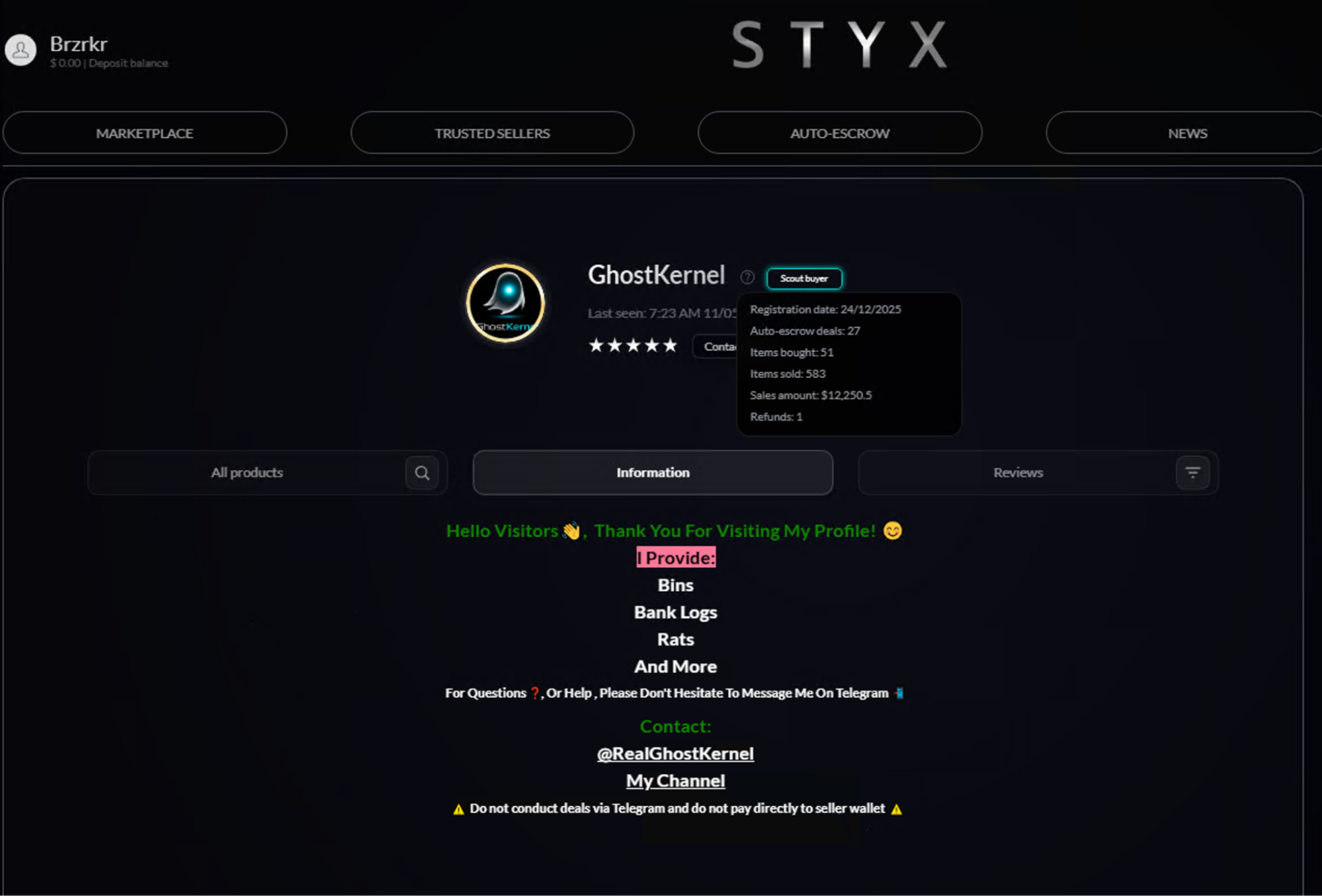
There are some notable differences between Styx and the rest of the reported marketplaces, however. Styx operates by offering sellers more space for promoting their own personal shops, available mostly through Telegram.
Figure 2 – Styx marketplace seller page
⠀
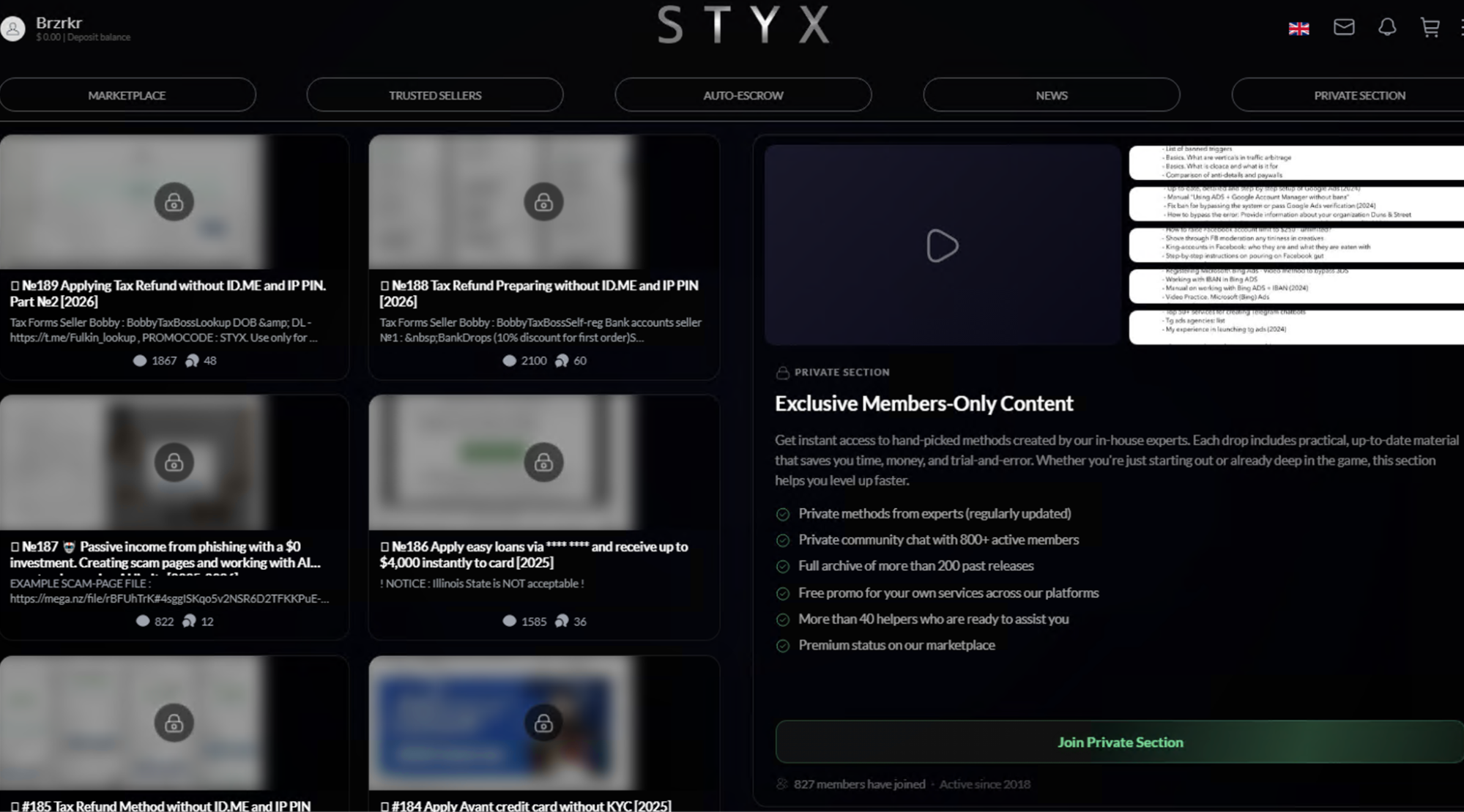
Styx also aims to cultivate a specialized community through their “freemium” model, where premium, high-value content is reserved for users willing to pay significant fees.
Figure 3 – Styx Marketplace Private Section
⠀
While some of the free manuals have been posted through different cybercrime forums before, they show not only a real attempt by the Styx admins to generate additional income, but also sell ad space for different sellers working outside of the marketplace. These monetization techniques indicate the admins are probably well aware they have many competitors, as they attempt to provide a different shopping experience for their users.
Resource development: Infrastructure
Infrastructure for cybercrime operations has been sold for a long time, offering adversaries illegal access to active domains, cpanels, and more.
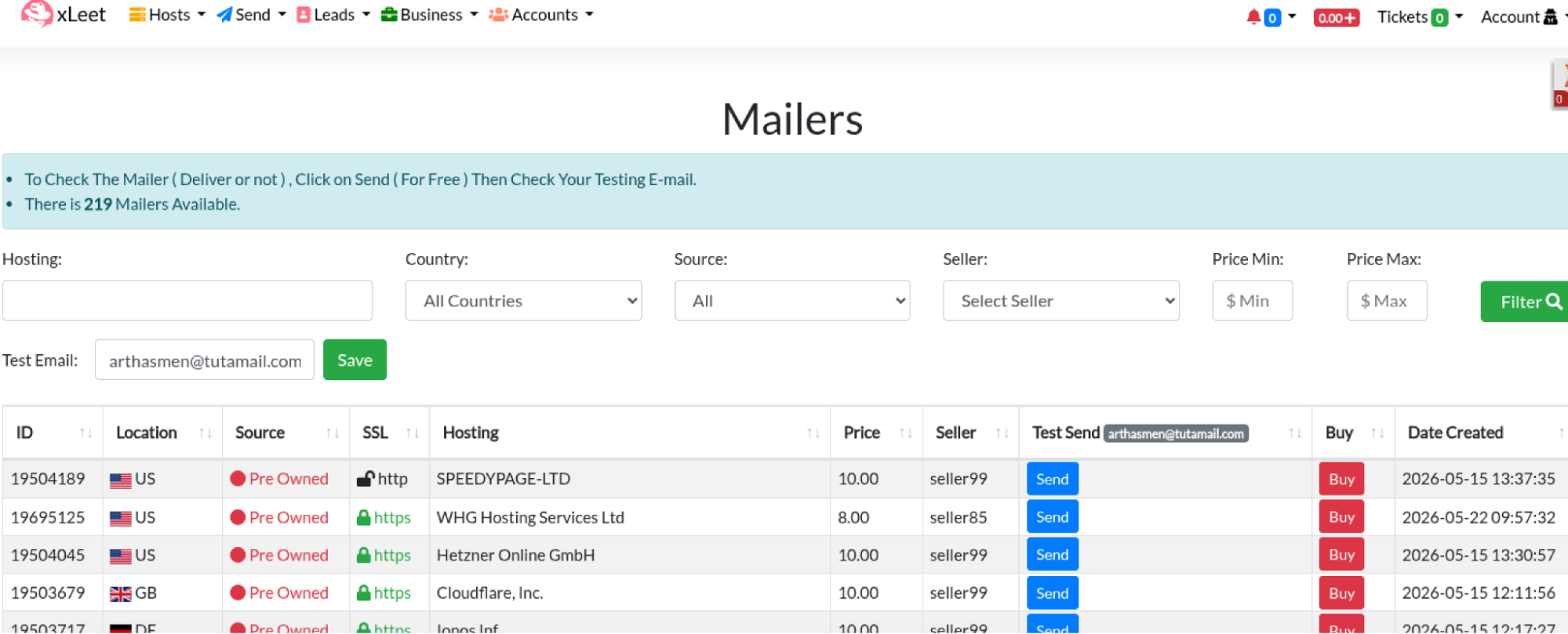
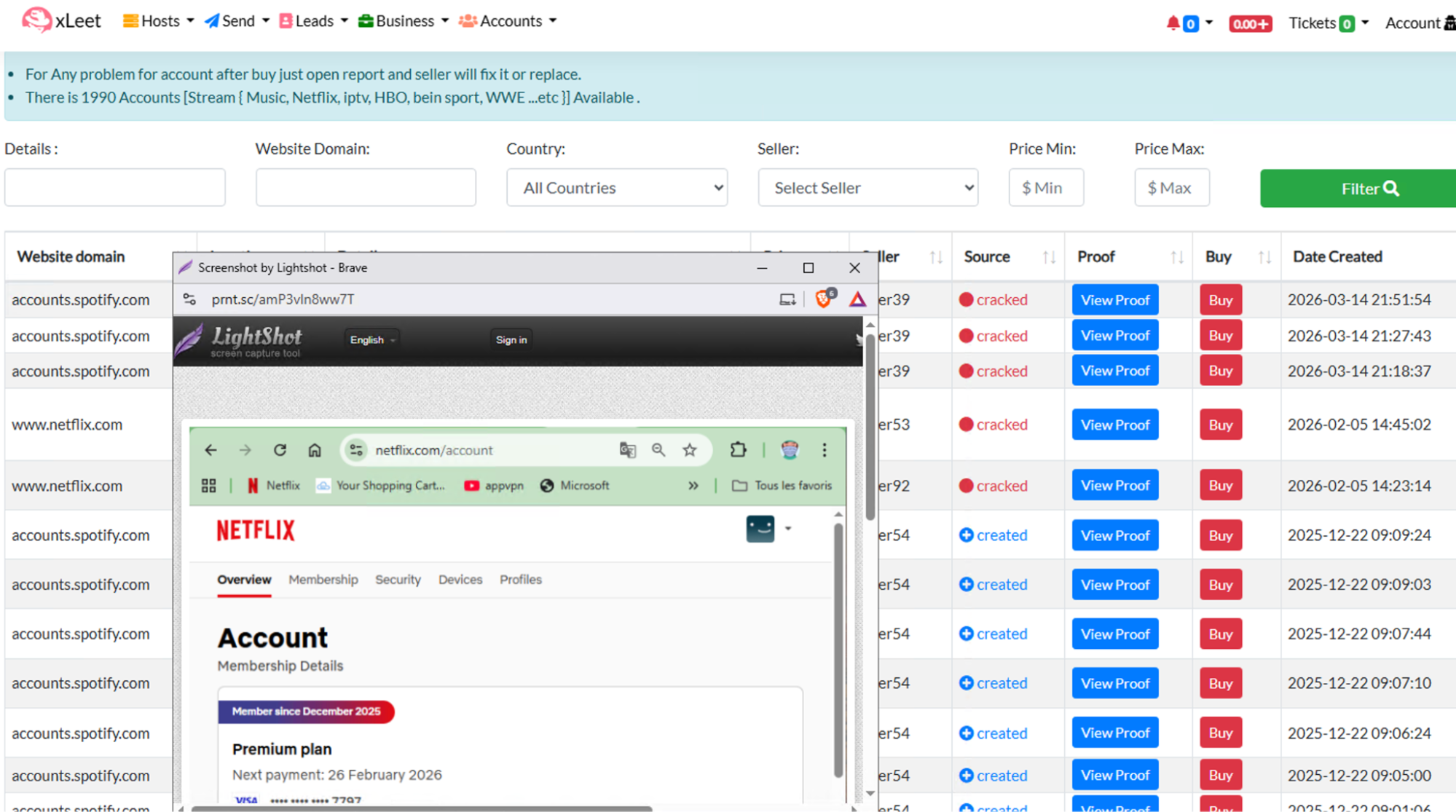
One of the leading marketplaces for such items is Xleet, first observed in 2022, which has quickly become a source for large collections of stolen credentials spanning multiple platforms. Distinguishing itself from other monitored marketplaces, Xleet is transparent about its offerings, frequently including evidence like screenshots or even email proof sent to the compromised account’s email address.
Figure 4 – Mailer infrastructure available for sale
⠀
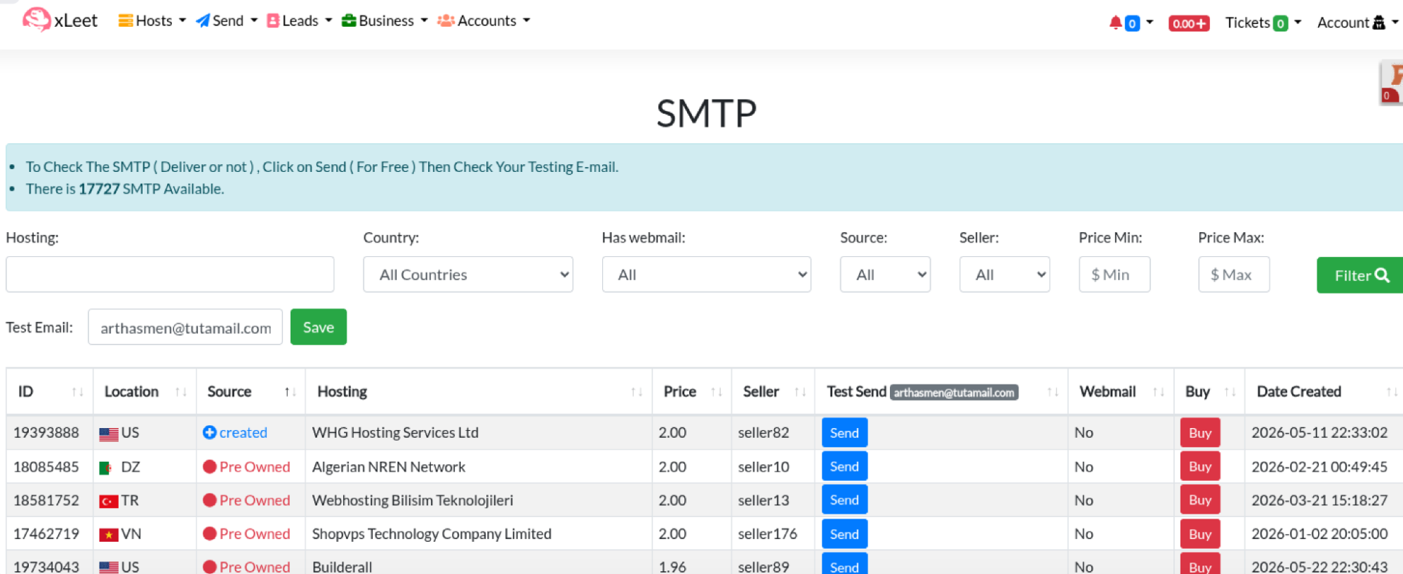
Figure 5 – SMTP infrastructure available for sale
⠀
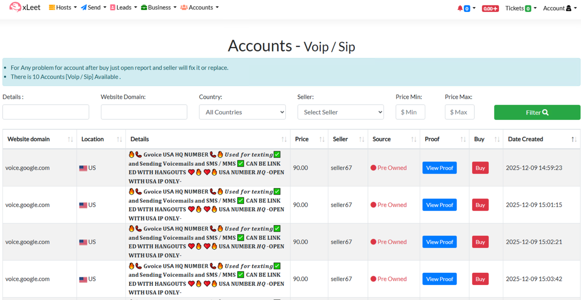
Access to SMTP servers could help fraudsters reach larger audiences and evade different email protection and filtering services, thus improving success rate for different schemes. Xleet also offers alleged access to protected networks through Cpanel, web shells, SSH, and RDP connections, as well as VoIP access through their accounts:
Figure 6 – VoIP access available for sale through Xleet
⠀
BlackPass is another marketplace offering RDP credentials, as well as proxy services used by malicious actors for veiling their location or, as mentioned above, bypassing different restrictions on their IP addresses.
Blackpass, initially named ‘Paysell,’ emerged as one of the first known online marketplaces dedicated to selling compromised accounts. Estimates suggest this platform has facilitated the sale of hundreds of millions of accounts. Legal documents indicate the marketplace is controlled by Russian cybercriminals, a detail consistent with its product focus: items exclusively targeting Western countries, particularly the US.
Figure 7 – Designated infrastructure for sale on Blackpass
⠀
All of these vulnerable environments could be part of a bigger scheme run by fraudsters, leading to other techniques being executed like a new vendor set up.
Another marketplace, Infodig, would offer different phone infrastructure in the past as mentioned in one of their opening posts on a cybercrime forum. Foreign or stolen numbers could be used for receiving or intercepting OTP messages, forging IT calls to employees, or self registering new accounts for other services.
Infodig has recently revamped some services offered, including the phone infrastructure, having been removed completely around the end of 2025 during an update the marketplace went through.
Figure 8 – Designated infrastructure for sale on Infodig
⠀
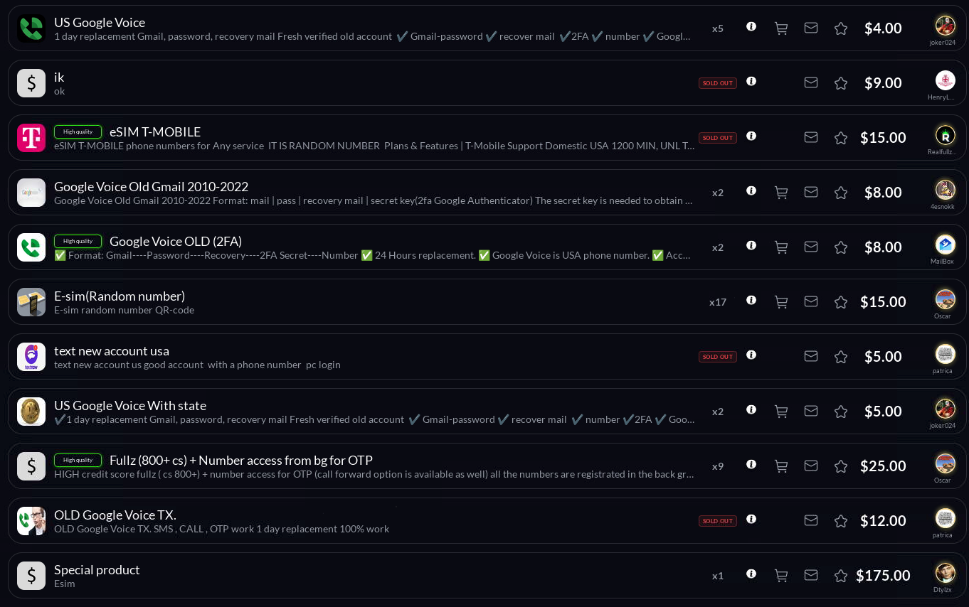
Styx also offers many options for fraudsters looking for ready to use infrastructure including eSIMs, VoIP services, and compromised VPN accounts. Localized SIM cards could be used by fraudsters for many reasons such as account creation but more importantly as a way to strengthen claims when confronting modern anti-fraud solutions, thus improving scam success rates.
Figure 9 – Styx VoIP and eSIM section
⠀
The same marketplaces offer additional stolen, forged, and even active company documents for sale including incorporation forms, US tax forms, and other various products connected to shelf companies and stolen PII. These documents allow threat actors to generate troves of mule accounts, shelf corporations, and even combine them into money laundering networks.
Acquiring access
Stolen, self-registered (self-reg), or user-sold accounts are high-demand assets in underground markets. By acquiring pre-existing accounts that have already circumvented anti-fraud protections, threat actors can rapidly deploy them for various criminal operations.
These platforms provide access to a wide range of services, from financial institutions and streaming providers to dating sites and AI-driven website builders. Novice fraudsters often utilize these resources to secure quick profits or to stockpile accounts for future resale.
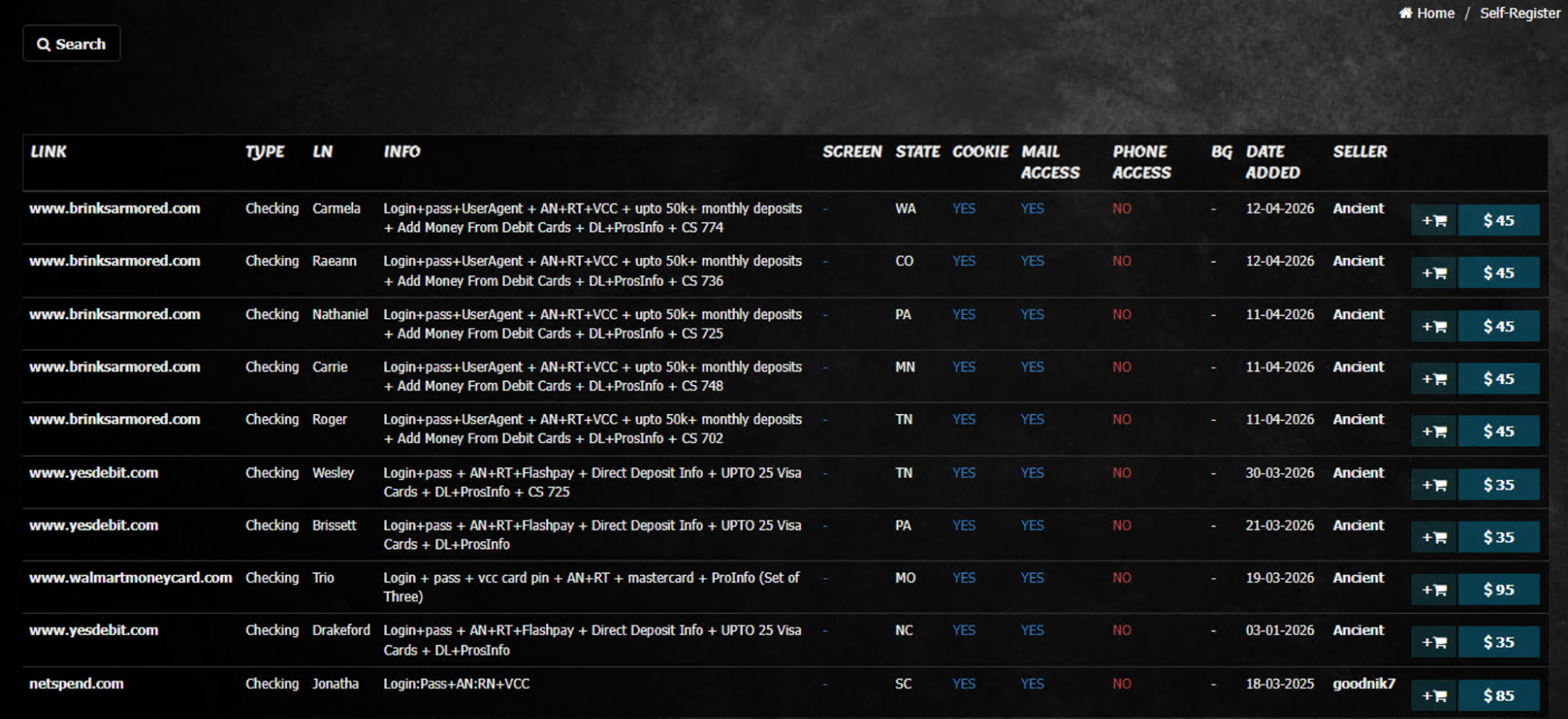
For example, Blackpass features an extensive account inventory that includes regional banks, neo-banks, and major corporations. Pricing within these markets is fluid; however, self-reg accounts typically represent the most expensive tier due to the significant labor required for their initial setup.
Figure 10 – Self-reg item available for sale
⠀
Xleet provides an extensive accounts division that covers a broad spectrum of common targets, including gaming, streaming, and dating service profiles. These specific credentials serve as high-value assets for executing various “pig butchering” fraud operations. Furthermore, a notable emerging trend within this marketplace is the significant surge in available credentials for AI platforms, especially those focused on accelerated website creation.
Figure 11 – Streaming accounts for sale, including proof
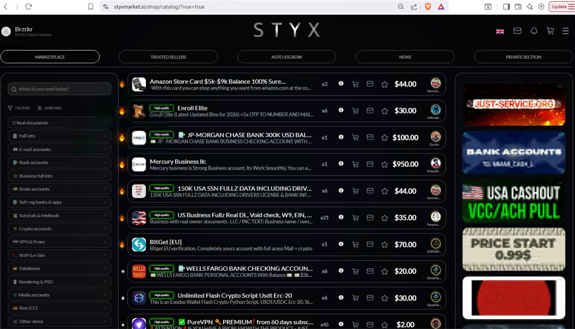
The newer type of marketplace, active since 2023, features an unorthodox design and much higher prices for their products. Styx holds the usual stock including stolen or self-reg accounts for a large variety of services, including financial institutions, social media accounts, streaming services, and casinos or other gambling sites.
Figure 12 – Styx marketplace
⠀
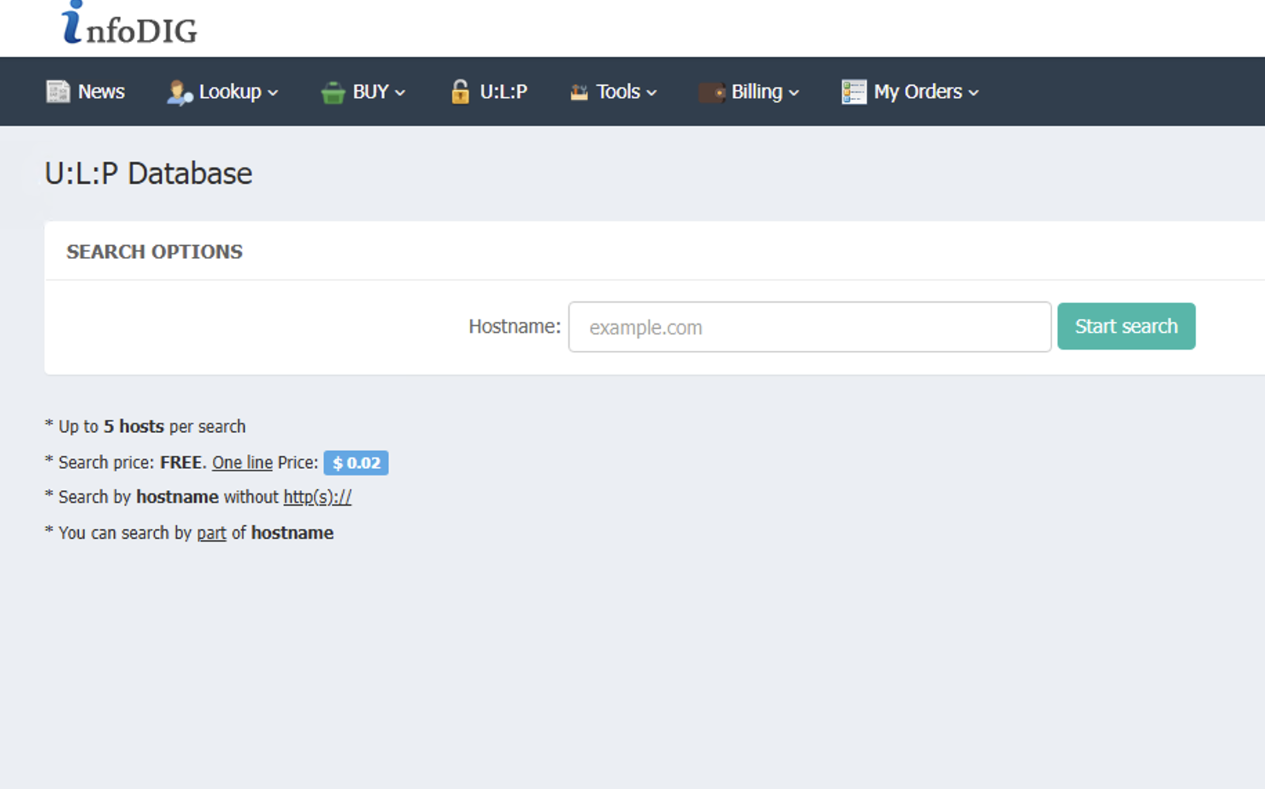
The inventory at Infodig is categorized into several distinct sections, featuring stealer logs alongside stolen Financial Information and Personal Identifiable Information (PII), such as Social Security numbers. Their accounts division has recently been going through some technical or supply issues and there are no current accounts available. However the marketplace has revamped their target list section into a new ULP (URL:LOGIN:PASS), offering a new targeted option for large scale ATO operations.
Figure 13 – New ULP section for Infodig
Monetization
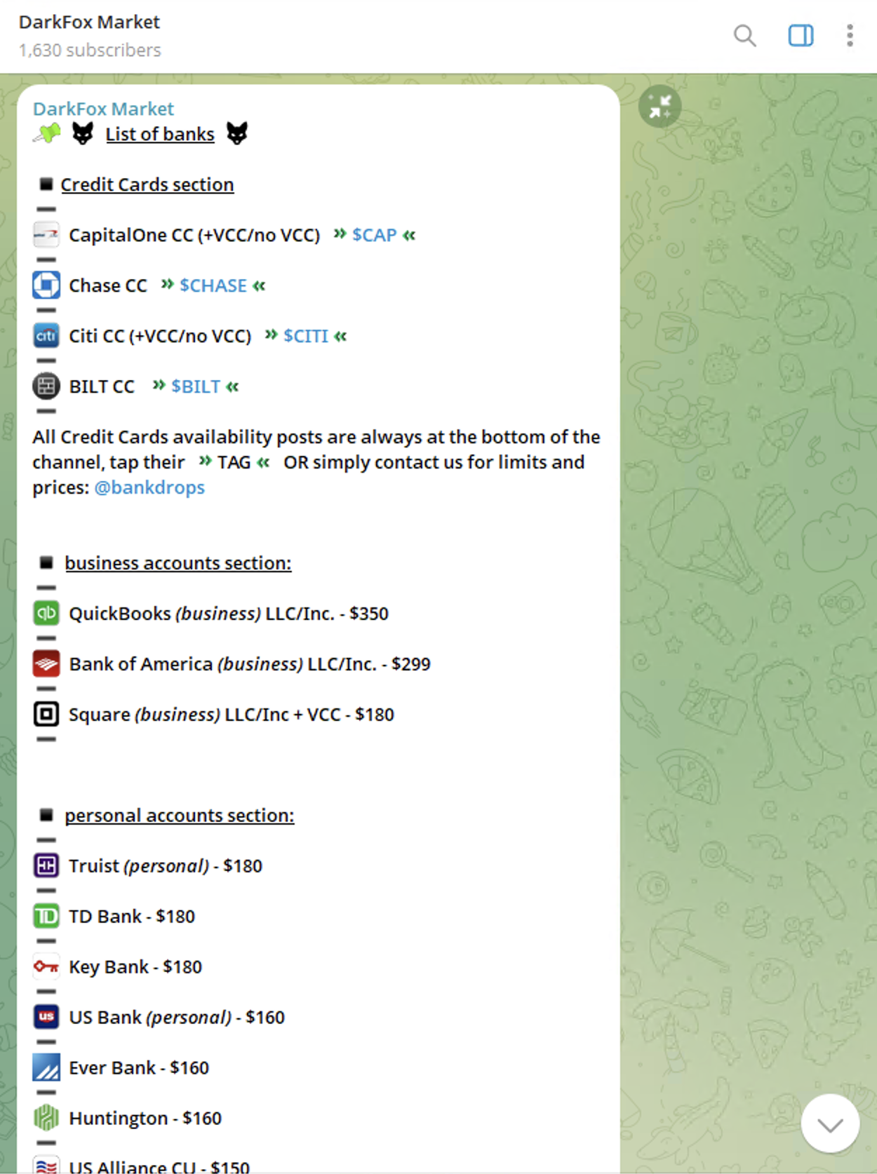
Styx has gained notoriety for its support of various “cashout” operations, which are prominently featured in numerous service advertisements throughout the platform.
By functioning as a hybrid of a marketplace and a forum, Styx provides a unique platform where merchants can offer specialized cashout services that exploit financial institutions across different payment rails. These merchants utilize various business accounts to assist fraudsters in laundering illicit funds through established methods, including payroll schemes, ACH transfers, and refund scams targeting multiple banks and geographic regions.
Figure 14 – Styx marketplace cashout ad
⠀
Beyond explicit solicitations for these services, marketplaces provide a variety of other products that are frequently exploited for money laundering. The exploitation of online gambling platforms remains a prevalent tactic for fraudsters, particularly as new regulations across the US lead to more states and companies entering the market. By acquiring stolen or synthetic PII, malicious actors can establish new gambling accounts to facilitate the laundering of illicit funds through techniques like chip dumping and minimal gameplay.
Conclusion
The fraud economy is changing at a fast pace with new techniques and players entering the field every day. By examining the different marketplaces portrayed in this blog post, we can see that they all react and appeal to different market needs.
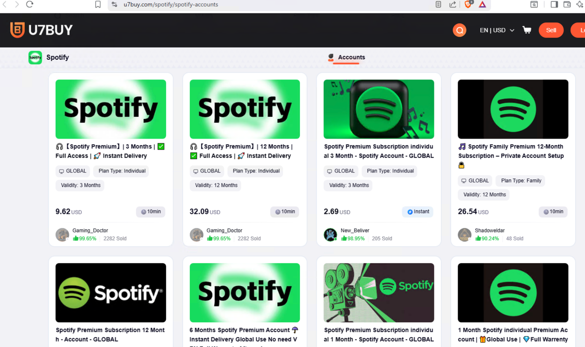
The change seen through available items across shops are a clear indication of this, as marketplaces pivot towards a larger crowd–one lacking the deep technical knowledge of the earlier fraudsters and carders. The different marketplaces allow every new fraudster to purchase their entire infrastructure for the fraud kill chain, from target lists, servers, and even support for laundering illegal income. Other online services include rapid AI creation of phishing threats, or other forms of abuse of legitimate service through stolen credentials. Marketplaces are not solely made for direct use and other threat actors view them as a major supplier for their shops as well, due to their fixed prices for items with prices which could easily be inflated through their personal shops as seen below:
Figure 15 – Specialized shop for streaming accounts
⠀
Figure 16 – Specializing account shop on Telegram
⠀
As fraud communities and groups become increasingly fragmented, the industry continues to splinter into smaller shops. These new, smaller marketplaces often require an invitation or administrator approval to join, a tactic designed to impede investigations and extend the lifespan of their fraudulent products. This shift to smaller shops also benefits merchants, allowing them to keep 100% of their profits instead of sharing them with marketplace administrators. Targeted companies should continue to monitor the marketplaces as they continue to function as an important link in the fraud supply chain. Threat actors are very aware and understand a major part of every business is the profit, therefore financial crime services and associated accounts are continuing to evolve.
Nevertheless, underground marketplaces will continue to operate as an important part of the cybercrime economic system. Smaller merchants may use these larger stores as suppliers for their smaller shops, as second income or even double or triple their income by selling the same stock in multiple locations. However companies should not only be aware of these underground ‘malls’, and regularly monitor them for any suspicious findings, but take a more proactive approach. The evolving nature of fraud demands a stronger reaction from organizations as well as cooperation from security, financial crime, and compliance teams for proactive measures against these threats.
Targeted companies, especially financial institutions or gambling providers, should actively investigate stolen accounts and gather vital intelligence for protecting themselves in the future, making it more difficult for threat actors to abuse their payment rails, brands, and customers.
What organizations should do
To safeguard both their infrastructure and clients, security teams must move beyond monitoring disparate data streams and actively align with internal fraud and financial crime units to cultivate actionable intelligence. Because illicit merchants rely on marketing their offerings, security analysts should actively communicate with threat actors, purchase account samples, as well as analyze images or videos to map threat actor networks, verify operational legitimacy, and finally deploy targeted security countermeasures. Threat actors are threatening organizations with more than just data exfiltration, with compliance or financial crime requirements, companies become more vulnerable to newer forms of threats, not commonly associated with security teams, but initiating through cybercrime sources.
By proactively identifying leaked assets, correlating them to their own environments, and responding quickly through credential resets, and fraud monitoring, organizations can significantly reduce both financial losses and downstream risks such as ATO, and money laundering.
Greg Kroah-Hartman has announced the release of the 7.2.5 and 6.18.51
stable kernels. There are more than 550 patches in each with fixes throughout
the tree; users are advised to upgrade.
Today, we’re making Cloudflare CASB more powerful than ever by introducing automatic remediation policies. This means security teams can now design event-driven logic to revoke risky file shares and dispatch custom webhooks, without manual intervention.
When we launched Cloudflare CASB, a cloud access security broker, we wanted to provide security teams complete visibility into the posture of their SaaS applications before misconfigurations became incidents. With a quick, clientless integration, CASB surfaces risks like overshared files, dormant admin keys and tokens, OAuth apps with excessive permissions — continuously, across users in the organization.
For years, SaaS Security Posture Management (SSPM) tools such as Cloudflare CASB have functioned as a passive alarm system. Most SSPM tools tell you what’s wrong but do not help you fix the issue, placing the burden on administrators to manage an ever-growing to-do list. A single misconfigured file-sharing policy across a Google Workspace tenant can generate thousands of findings in seconds, and even a disciplined team faces a window between detection and remediation measured in hours or days — more than enough time for a sensitive file to be downloaded, forwarded, or indexed.
With automatic remediation policies, CASB customers can now configure the actions that should be invoked immediately after a new finding is identified.
Shifting from reactive to proactive
When we launched manual remediation actions earlier this year, we gave security teams the ability to resolve misconfigurations directly from the Cloudflare dashboard. This removed the need for customers to log in to multiple SaaS portals to take action on the security and content findings detected by Cloudflare CASB. Still, this required a human to confirm and initiate each individual remediation — even if they’d seen this exact finding type before.
CASB policies are a native automation engine built directly into Cloudflare One that takes action the moment a finding is detected. Security teams define their response logic once, whether that is revoking access to a file share, dispatching a webhook to your security operations center (SOC), or forwarding the event to a security orchestration, automation and response platform (SOAR). The engine handles matches automatically by executing the customer-configured action.
As an example, many organizations implement controls that prohibit files from being shared publicly. However, they may apply an exception to users and groups in their marketing department who are frequently required to collaborate with external parties. SSPMs allow their customers to be alerted of any files that are shared publicly in violation of their policy. With many solutions, this permitted behavior lands in a queue with hundreds of possible violations, forcing administrators to take action on each individual instance.
CASB policies are designed for exactly this scenario. Rather than waiting for a human to see and act on a finding, automation fires the moment detection happens. The public share is revoked within minutes, keeping the backlog of findings clean and clear.
How CASB policies work
At their core, CASB policies are automated workflows that tell our scanning service what action to take when a new finding is detected. From there, the configured policy will tell CASB to either trigger a remediation action, send a webhook, or both. This gives organizations the flexibility to rely on native CASB remediation capabilities or their own internal automation services and communication channels — without having to take action in disparate platforms or create their own event processing system.
How we built it
The architecture behind CASB policies is built entirely on the Cloudflare developer platform — the same platform available to every Cloudflare customer.
When a finding is detected, the findings engine enqueues an orchestration message to a Cloudflare Queue. A Worker consumer then checks whether a policy configuration matches the incoming finding. If a match exists, it creates the corresponding job and hands it to the remediations pipeline, which runs on Cloudflare Workflows for durable, fault-tolerant execution. That means jobs survive process restarts and retries are handled automatically.
Cloudflare Workflows also handle third-party API rate limits gracefully. If a vendor returns a rate limit error, the Workflow pauses for the appropriate backoff window and retries without dropping the job. Our target from detection to completed remediation is five minutes or less.
How to create policies
To get started, navigate to the Cloudflare dashboard and create your first policy. Policies can include both a remediation and a webhook action, but at a minimum:
Select the vendor. Select the vendor and integration or tenant this policy should apply to.
Select the integration. You can hand-select specific integrations or set it to apply to all integrations for the selected vendor.
Choose a finding type. Select the CASB finding type that should fire the policy.
Choose an action. Once a trigger is selected, the available actions for that finding type are shown. There are two categories:
Run remediations. First-party actions Cloudflare performs directly against the SaaS integration API. CASB currently supports remediation actions for Microsoft and Google Workspace file/folder finding types. Note that this may require upgrading permissions on integrations to read/write.
Send webhooks. Send finding details to configured webhook destinations such as Slack, Microsoft Teams, Jira, ServiceNow, Tines, or any custom HTTP endpoint your team uses.
Example webhook format
Maintaining visibility and compliance
Each policy action produces two categories of logs, visible under Insights in Cloudflare One.
Admin Activity logs. These capture changes to a policy definition: who created it, who edited it, who disabled it, and when. If a policy was turned off and a risk slipped through, this audit trail surfaces a timeline of the event.
Cloud & SaaS Security policies logs. This new class of logs captures the runtime outcome of policy invocations. This includes details like which finding triggered the policy, which file was acted on, whether it succeeded or failed, and the specific error if it did not — for example, a 401 Unauthorized or an API rate limit response from the vendor.
For compliance use cases, the execution log is the proof of fix. It ties a specific finding, like an overshared file (e.g. Q4_Financials.pdf), to a specific automated action and event timestamp.
Get started
Customers can find CASB Policies in the Cloud & SaaS findings section of the dashboard today. Connect or update your Microsoft 365 or Google Workspace integration to Read-Write permissions, and create your first remediation policy.
In the coming weeks, we’ll also be adding support for Custom Findings to CASB. Different organizations have unique needs when it comes to detection, and we want to give customers the ability to augment or define finding logic to fit those needs.
Концепцията, че майката е не просто обгрижващ възрастен, а източник на обич за бебето или малкото дете и ключов посредник между него и света, е описана научно за първи път през 40-те години на ХХ век. Тогава редица наблюдения на педиатри и психиатри водят до идеята, че дори безупречното задоволяване на медицинските и физиологичните нужди на едно бебе или малко дете не може да предотврати негативите от институционалните грижи и че връзката с обгрижващите възрастни всъщност е неделима част от развитието на детето. Оттогава теорията е изследвана и прецизирана през годините и днес стои в основите на семейно ориентираните грижи, включително в практиките, които насърчават родителското присъствие по време на болнично лечение на деца.
В България обаче все още често нуждата от лечение става причина за разделяне на семейства. Това се превръща в особено сериозен етичен въпрос, когато става дума за продължително лечение или за грижи в края на живота. Причините са сложни и обхващат както остарялата и неподходяща инфраструктура, така и остарелите практики и нагласи.
Зад всички сложни проблеми обаче стоят човешки истории. В случая – най-тежките, които героите на тези истории са преживели.
Елица*
Срещам се с родителите на Елица пред входа на центъра за настаняване от семеен тип, в който тя живее, а те я посещават почти всекидневно. Носят голяма чанта с вещи – активна гимнастика, играчки, консумативи. Познах родителите отдалеч, макар никога да не ги бях виждала.
Елица е на две години. Дълго чакано дете от следена под лупа бременност. Ражда се обаче с множество проблеми, които изискват както редица активни медицински интервенции, така и постоянни специални грижи.
До последно смятахме, че всичко ще е наред. Бяха ни казали само, че може да е с по-ниско тегло. Първия път, когато ми я дадоха, я бяха повили и почти нищо не се виждаше от нея. По-късно я взеха и едва тогава разбрах всичко,
разказва майката. Елица има лицеви изменения, които са добре познати на медицината. На популярен език се наричат заешка устна и вълча уста. Наред с тези иначе решими проблеми обаче момиченцето има аномалии на опорно-двигателния апарат, както и на вътрешните органи, заради които лекарите прогнозират, че ще живее не повече от две седмици.
„Бяхме в шок“, споделя баща ѝ.
Двете седмици обаче отминават, бебето преживява животоспасяваща коремна операция и след още известно време, прекарано в отделението по неонатология, социалните препоръчват, а съдът решава официално да изведат Елица от семейството и да я настанят в Център за настаняване от семеен тип. Аргументът е, че там може да се полагат медицински грижи за деца в тежко състояние и момиченцето ще има шанс да наддаде на тегло, да се стабилизира и да се извършат поредица от операции, които да направят живота му възможен. Центърът за настаняване е в друг град, на около 200 км от дома на семейството. „Ходехме да я видим всеки вторник“, припомня си бащата. „Освен един, когато имаше грип. Тогава я видяхме само през стъклото“, допълва майката.
Докато ми разказват историята си, родителите си играят и паралелно говорят с малката Елица. Тя не изглежда като повечето двегодишни деца. През носа ѝ минава тръбичка – това е сондата, през която се влива специалната медицинска храна. Момиченцето е по-малко, едва около 7 килограма, а ръцете и крачетата му не са развити както на повечето му връстници.
Но когато баща му говори – тихо и бавно – то го слуша с огромно внимание.
Питам ги дали ги разпознава. „О, да. И не само това. Преди идвахме вечер след работа, към 5 часа. Сестрите казват, че като наближи този час, започва да се върти“, разказва бащата. „Чака ни“, пояснява майката и започва да закача детето: „За теб говорим, мамо…“
Как си говорят Елица и нейните родители – малък момент на нежност в едно кратко аудио:
Разговорът ни се провежда в центъра за настаняване от семеен тип, в който Елица е преместена преди около година от по-далечния град. Този е само на няколко километра от селото на родителите, а екипът подкрепя семейството да бъде заедно колкото може повече. С активното им съдействие родителите получават разрешение от Отдела за закрила на детето дъщеря им да гостува в семейния им дом. И все пак посещенията на Елица в дома на собственото ѝ семейство са рядкост. Надеждата на родителите е, че дъщеря им ще укрепне достатъчно, за да бъде оперирана и да започне да се храни без сонда – това е пътят ѝ към прибиране у дома.
„Гледането е тежко“, отбелязва някак неочаквано майката, а бащата допълва: „Проблемът е, че за деца с тежки увреждания няма много варианти – например дневен център, където да можеш да го заведеш през деня… и може би ще бъде много трудно…“
Ще бъде много трудно, аз вече съм го осъзнала,
слага точка на емоционалното отклонение майката. Двамата се връщат към практическите въпроси около организирането на операциите на малката Елица. „Това много се проточи, бавно става – споделя баща ѝ. – Просто искаме да си я вземем у дома.“
С Диана се срещам, за да проведа най-трудния разговор – този, в който родителите си вземат у дома само въпросите и съмненията. Аз задавам твърде малко въпроси – майката има достатъчно. Историята се излива от Диана, сякаш в последните месеци само е чакала някой да бъде там, за да я чуе:
„Много ми е противоречиво все още усещането дали имам свободата да разкажа за това, което ни се случи, защото имах близначета. И историята с двамата е много различна. Знам, че има родители, които са изгубили единственото си дете, и за тях е още по-тежко. Аз имам и едно по-голямо дете и успявам някак си да разделя тези две вселени. Едната вселена е нашето ежедневие, в което аз имам моите две момчета, за които да се грижа, които да обичам, и мога да функционирам нормално. Другата са моментите, в които мога да притихна, в които съм сама, и тогава преминавам отново през всичко, което се случи.
Близнаците ми се родиха преждевременно, почти в 34-тата седмица. Малкото ми момиченце Ида се роди първо. Тогава не разбрах, че се е наложило реанимиране – аз чух проплакването и след това я отведоха, без да ми я покажат дори. Минута по късно се появи малкото ми момченце Йоан. Видях го за секунди, след това отнесоха и него.
Часове по-късно се появи една лекарка, която ми се скара защо съм тръгнала да раждам в тази болница, в която неонатологията не е на необходимото ниво. Трябваше да дам съгласие да извозят малкото ми момиченце към специализирана неонатология с повече възможности за поставяне на сърфактант. След още известно време я доведоха с креватчето, за да си я видя. Това беше първата ни среща, но тя спеше, а аз бях все още на легло, не успях дори да я докосна, преди да я преведат в другата болница. По-късно преведоха и Йоан.
Близо седмица се обаждах всеки ден за информация. След като ме изписаха, една събота беше, ги видяхме, като тогава не беше ден за свиждане. Мънички ми се сториха, безкрайно най-сладките и красиви бебчета. Дори не ми мина през ума да попитам дали мога да си ги пипна по ръчичките… Просто ги гледахме.
На следващия ден ми се обадиха. Ида беше получила гърч. След това изпадна в кома. Тази кома продължи пет месеца и няколко дни.
И така, в първите може би 6–7 дни повечето лекари там подаваха някакъв вид успокоение, че е възможно комата да е и заради успокоителните. След като направихме образно изследване на мозъка обаче, стана ясно, че е пострадал необратимо. И след това за мен започна едно продължително свободно падане в някакво неясно пространство. Сякаш нямах силата да попитам и да ми обяснят малко повече, тоест беше едно такова просто дълго изчакване без яснота на какво мога да се надявам.
Йоан го изписаха някъде на 40-тия ден. Давам си сметка, че те се опитваха да ги задържат близо един до друг. Тоест наистина имаше някакви неща, които усещах, че правят отвъд медицината, за да има някакво успокоение и за нас като родители, и за тях двамата. Въпреки стъклената преграда на кувьозите се опитвах да давам цялата си обич и знам, че и бебчетата ми го усещаха.
Лекарите от неонатологията ми позволяваха да оставям малки предмети и играчки в кувьоза – осветени дрешки, икона, играчки, подаръчета за Коледа, музикална парцалена кукла, която Дядо Коледа подари на Ида, ангелче. Разбира се, винаги пакетирани в стерилизиран плик. Опитвах се да бъда най-добрата възможна майка за малкото време, което имахме заедно.
И обичта беше там.
Това беше един голям урок по сила и обич, който с малката ми Ида споделихме. Вечер си представях, че я погалвам, че съм до нея и ѝ пожелавам главичката и сърчицето ѝ да са здрави, изпращах обич и знам, че усещаше това.
Ходех на регулярните свиждания два пъти седмично, които са по около час. Тогава и всички други родители на бебенца в отделението са там, а лекарите минават и дават информация. Опитвах се да ходя и още веднъж-два пъти в седмицата в някакви следобедни часове през уикендите например, в повечето случаи са ме допускали. Все пак се съобразявах кой е дежурен лекар, и не стоях дълго.
Вече беше може би на третия месец, когато видях, че една от сестрите безкрайно нежно и опитно погалва и гушка в кувьоза и другите бебчета, както и моето. И всъщност това беше моментът, в който си дадох сметка, че мога да не подавам само ръчичката, а може би мога да я погаля по главичката. Но разговорът докъде може да стигне контактът помежду ни всъщност никога не е воден. Това може да е моя грешка, мой пропуск. Но просто когато наистина всеки ден по телефона чуваш колко е сериозно положението, се страхуваш да не навредиш.
Точно на Нова година бяхме с мъжа ми при кувьоза и тогава при нас дойде заместник-директорът на болницата. Имахме ужасен разговор. Той ни намекна, че трябва да решим какво да правим, защото това може да продължи твърде дълго. Че в някакъв момент може да започнат да се образуват декубитални рани и да е много тежко да се гледа. Този разговор не бива да се случва така на никое семейство, на такова място, по този начин…
Ние всъщност до този момент не бяхме осмислили какво означава „много лоша прогноза“, макар някои от лекарите да бяха опитали да ни намекнат, че в един момент сърчицето ѝ ще се предаде.
В деня, в който се случи най-лошото, беше обявена някаква грипна ситуация. От отделението ми казаха, че предпочитат да не ходя, но аз настоях, защото бях ваксинирана.
Всъщност слава богу, че отидох, защото постоях малко по-дълго време. Имаше едно потрепване на очичките, особено когато я погалвах, и мисля, че наистина си беше някакъв вид реакция на душичката, че съм близо до нея.
Когато отидохме в деня, след като Ида отлетя, всъщност беше първият път, в който я прегърнах. Нещо, от което през цялото време много ме беше страх, и се чудех дали ще намеря силата да го направя. Но всъщност дори не се замислих. Това беше най-правилното и истинско нещо, което можех да направя в този наш път заедно.“
Христо
Никое общество не е изградило система, която да подготвя родителите да погребват децата си, защото това противоречи на естествения ход на живота. Но всичко е много различно, когато тези хора получават подкрепа в процеса,
казва Христо към края на интервюто ни. Той е лекар. Млад лекар, защото в тази професия се учи дълго, затова се остарява бавно. Христо е известен като д-р Христов и е анестезиолог, работи като детски анестезиолог и реаниматор, бил е най-младият координатор по донорство. Говорим с д-р Христо Христов как в една недружелюбна система да се намери балансът между нуждата от медицински грижи и нуждата от родителска подкрепа на децата пациенти, когато липсват условия да бъде откликнато едновременно и на двете. Особено когато тези пациенти са в края на живота си.
„Аз съм работил в интензивно отделение, където родителите са придружавали детето, и беше много хубаво“, разказва д-р Христов. По думите му, това е по-скоро изключение, тъй като в повечето лечебни заведения нито интензивните отделения са пригодени да посрещнат придружител, нито медицинският екип се чувства спокоен да работи в присъствието на родител. Според анестезиолога липсва опит с тази практика:
Всъщност родителите са спокойни, защото знаят какво се случва с детето им, какво правим, то спало ли е, яло ли е, боли ли го, тъжно ли е – родителят е там и вижда, и може да бъде от полза за детето си.
Доверието между родители и медици е компрометирано, смята д-р Христов, и това създава допълнителни пречки. „Много лекари в България не са виждали грижа за пациента вкъщи и не вярват, че такава грижа може да бъде полагана както трябва“, смята той. „Имаше едно дете, което беше престояло в болницата две години – разказва още лекарят. – Колегите бяха осигурили апаратура, с която да може да си отиде вкъщи, но не намираха сили да го изпратят у дома, защото ги беше страх, че вкъщи то ще умре.“
Тази история завършва с успешното събиране на семейството. Пътят минава през упорита работа на екипа с родителите, за да се обучат и да могат в своето село, на часове път от лекуващия екип, да отговарят на нуждите на детето си. „Да, това дете ще трябва да влиза в болница. Няма да е лесно. Но ще има качествено време у дома със своето семейство“, убеден е д-р Христов.
При тежки състояния, когато медицината изчерпи възможностите си за активно лечение и стане ясно, че повече нищо не може да се направи за излекуването на едно дете, фокусът на грижите се измества към неговото семейство. Според д-р Христов, когато едно заболяване е в терминален стадий или е настъпила мозъчна смърт, медиците трябва да бъдат честни с близките, да ги подготвят и да им осигурят време, подкрепа и възможност да прекарат последните си часове заедно в спокойствие и с достойнство. „Имали сме случаи, в които сме чакали някой от семейството да се прибере от чужбина. Или да го обсъдят помежду си, да съумеят да го осмислят и да се сбогуват“, споделя той.
В много случаи обаче такова време „заедно“ просто няма как да се осъществи пълноценно в нашата система. „Общественият разговор, който липсва, е какво всъщност е в най-добрия интерес на детето, когато медицината не може да го излекува – дали да прекара останалата част от живота си в кувьоз, или в болнична стая, защото това би му осигурило повече дни, или да има по-малко време, което обаче да прекара със семейството си. Този въпрос няма лесен или еднозначен отговор, но за да бъдем честни към семействата, трябва да започнем да го поставяме.“
Месец и половина преди осмите преки президентски избори българските граждани знаят имената на кандидатите. Но знаят ли какъв президент избират? „Обединител на нацията“, както твърди политическото клише? Церемониалмайстор на държавата? Или коректив на властта, от когото се очаква да вижда по-далеч от следващия бюджет и следващото правителство?
Когато през 1990 г. Националната кръгла маса обсъжда създаването на президентската институция в новата конституция, отрежда на държавния глава далеч по-съдържателна роля. Той трябва да бъде „арбитър и гарант“ за нормалното функциониране на държавата, националната сигурност, териториалната цялост и международните ѝ ангажименти, казва Георги Пирински (БКП). И още: да пази баланса на интересите и правовия ред в полза на всички граждани, а не на отделна част от тях.
Тогавашният представител на СДС Крум Неврокопски добавя друго определение: президентът е „гарант и арбитър за националното съгласие“, но и „гарант за бъдещето“ – фигура, призвана да утвърждава посоката напред и да осигурява мирния преход към демокрация. Така е замислена институцията в началото – като гарант, че политическото противопоставяне няма да разруши държавата и нейното бъдеще.
В Конституцията обаче президентът не е наречен нито обединител, нито арбитър. Според чл. 92 той е държавен глава, който „олицетворява единството на нацията“. Глаголът олицетворява е важен:
президентът не е натоварен да създава единство там, където има различни убеждения и политически конфликти, а да представлява нацията като цяло – включително и гражданите, които не са гласували за него.
Още през 1995 г. Конституционният съд пресича удобното тълкуване, че държавният глава трябва да стои безмълвен и равноотдалечен от всички. „Националното единство не означава политическо единомислие“, се казва в Решение №25. Президентът не е деполитизиран орган: той има право да заема позиции, да отправя политически послания и да издава актове със съществени политически последици. Неговата надпартийност не е безразличие, а задължение да преценява властта и политическите конфликти от гледна точка на Конституцията и интереса на цялата общност, а не на партията, която го е издигнала.
„Длъжностната характеристика“ на практика
Петимата президенти след началото на демократичните промени влизаха на „Дондуков“ 2 в различна България, а и с различна представа каква посока да отстоява държавата. Представите им се формираха от политическите сили, които ги излъчваха, но и от техните убеждения и зависимости.
Първият пряко избран президент Желю Желев не произнася програмна реч при полагането на клетвата си през януари 1992 г. – само подписва клетвения лист. Неговата заявка обаче е зададена още от биографията и политическата му роля: демонтиране на тоталитарната държава, утвърждаване на парламентарната демокрация и връщане на България към Европа.
Желев: коректив и „Боянски ливади“
Философът и един от водачите на демократичната опозиция Желев показа как президентът може да бъде коректив на политическата сила, която го е издигнала. Но „Боянските ливади“ оставят открит въпроса къде свършва корективът и откъде започва намесата в управлението. На пресконференцията от 30 август 1992 г. той обвини кабинета на Филип Димитров, че е влязъл в конфликт с медиите, синдикатите, Църквата, Президентството и извънпарламентарните сили. Два месеца по-късно правителството на „сините“ изгуби поискания вот на доверие, след като ДПС и част от депутатите, избрани от СДС, отказаха подкрепа.
Намесата на Желев задълбочи разцеплението и придаде институционална тежест на атаката срещу кабинета. Следващото правителство на проф. Любен Беров, подкрепено от БСП и ДПС, не донесе нито по-голяма прозрачност, нито по-убедителни реформи. Затова „Боянските ливади“ остават двусмислен епизод: доказателство за независимостта на президента от собствената му политическа среда, но и предупреждение, че корективът може да разклати властта, без това да е от полза за демократичния преход.
Националният хоризонт при Желев беше по-ясен от вътрешнополитическите му маневри: демокрация, европейска принадлежност и излизане от съветската орбита. През февруари 1994 г. той подписа рамковия документ за включването на България в програмата на НАТО „Партньорство за мир“ – първата институционална крачка по пътя към членството в Алианса.
Стоянов: посоката е ЕС и НАТО
При юриста Петър Стоянов ролята на президента като коректив и носител на национален хоризонт се прояви още преди официално да встъпи в длъжност. Той положи клетва на 19 януари 1997 г. в държава с хиперинфлация, масови протести и рухнало доверие в управлението на БСП. В първата си реч поиска предсрочни избори, валутен борд и „нова воля за промяна“. Но най-важната му заявка беше посоката: България трябва да избере „европейския тип цивилизация“ и интеграцията в Европейския съюз и НАТО.
Две седмици по-късно Президентството се оказа в центъра на политическата криза. На 4 февруари 1997 г., след заседание на Консултативния съвет за национална сигурност и преговори между основните политически сили, БСП върна мандата за съставяне на ново правителство. Последваха служебен кабинет и предсрочни избори. Стоянов не изведе сам България от кризата, но използва авторитета и инструментите на президентската институция, за да предотврати продължаването на управление, изгубило обществена легитимност.
Неговият хоризонт беше формулиран ясно: върховенство на закона, пазарна икономика и необратима принадлежност към ЕС и НАТО. Това беше и мярката, с която Стоянов оценяваше текущата политика. В момент на дълбоко разделение той не обедини всички около общо мнение. Помогна да се постигне съгласие накъде да върви държавата.
И макар да беше избран с гласовете на избирателите, довели на власт и ОДС, и кабинета на Иван Костов, отново настъпи разрив между него и изпълнителната власт.
Първите признаци се появиха още през 1998 г., когато Стоянов започна да критикува кадрови решения и начина, по който СДС упражнява властта. До открит сблъсък се стигна през април 2000 г., след обвиненията на уволнения вътрешен министър Богомил Бонев за корупция във властта (Бонев беше отстранен поради съмнения за същото). Стоянов упрекна премиера, че не обяснява причините за смените в правителството от декември 1999 г.
Последва разгром на сините на изборите през 2001 г., когато отношенията между премиер и президент фактически бяха прекъснати. Стоянов се кандидатира за втори мандат като независим, макар и подкрепен от ОДС, и загуби, а Костов подаде оставка като лидер на СДС.
Първанов: прегръдка с капитала
Единственият политически лидер, избран за президент – председателят на БСП Георги Първанов, встъпи в длъжност през 2002 г. Закле се в името на „националното помирение и съгласие“. След ожесточеното противопоставяне на 90-те години той предложи друга представа за Президентството – посредник между политическите сили, и даже се самоопредели като „социален президент“.
По време на двата му мандата България постигна двете големи цели на Прехода – членството в НАТО през 2004 г. и в ЕС през 2007 г. Първанов не беше техният архитект, но Президентството му осигури приемственост във външнополитическата посока.
Договореният между него и Путин „Голям шлем“ от руски енергийни проекти не се превърна в национален хоризонт, а в източник на зависимости, политически спорове и провал. По изчисления на „Капитал“ „България пропиля поне 2,3 млрд. лв. в трите лошо обмислени енергийни проекта [АЕЦ „Белене“, газопровода „Южен поток“ и нефтопровода „Бургас–Александруполис“ – б.а.]“.
На 17 септември 2001 г. – по-малко от два месеца преди президентските избори – беше учреден бизнес клуб „Възраждане“. Сред основателите му бяха някои от най-могъщите фигури на Прехода: банкерът Емил Кюлев, президентът на „Мултигруп“ Илия Павлов и Васил Божков. В следващите години първите двама бяха убити от неизвестни и до момента извършители.
Кюлев, който оглави клуба, след победата на Първанов стана и негов икономически съветник. Така още в началото на мандата около „социалния президент“ се оформи кръг, в който политическото влияние и едрият капитал се срещаха без особена дистанция. По-късно от американска дипломатическа грама, разпространена от WikiLeaks, се разбра, че Кюлев е финансирал кампаниите на Симеон Сакскобургготски и Първанов.
Близостта не се изчерпваше с „Възраждане“. Сред официалните спонсори на кампанията на Първанов за втори мандат фигурираха и фирми на Людмил Стойков – бизнесмен, чието име се появи в разследването на ОЛАФ за злоупотреби със средства по САПАРД.
Това показва парадокса на Първановото „помирение“: президентът, който обещаваше да представлява губещите от Прехода, отвори Президентството за хората, спечелили най-много от него. Така социалната реторика започна да служи като прикритие на близостта между властта и едрия капитал.
Дали не виждаме същата хамелеонщина и при Румен Радев?
Днес Първанов е един от хората в инициативния комитет, издигнал настоящата президентка Илияна Йотова и генералния директор на БТА Кирил Вълчев за президент и вицепрезидент.
Плевнелиев: с план за бъдещето
Предприемачът Росен Плевнелиев дойде през 2012 г. със заявката да бъде „прагматичният президент“. Неговият речник беше различен: модернизация, конкурентоспособност, образование, електронно управление, иновации, енергийна независимост.
Той опита да превърне Президентството в място за изработване на дългосрочни приоритети чрез националната програма „България 2020“ и чрез обществените съвети към институцията. Във встъпителното си слово обеща Президентството да бъде отворено за гражданите, защото „президентът не е началник на гражданското общество“.
Политическите кризи след 2013 г. го превърнаха и в коректив. След избухването на протестите #ДАНСwithme, предизвикани от избора на Делян Пеевски за шеф на контраразузнаването, Плевнелиев застана срещу кабинета „Орешарски“. По време на мандата си той назначи две служебни правителства, защитаваше категорично европейската принадлежност на България и осъди руската анексия на Крим.
Избран с подкрепата на ГЕРБ, Плевнелиев имаше хоризонт, но не и политическа тежест. В рамките на президентския си мандат изработваше стратегии и защитаваше позиции, които така и не станаха част от дневния ред на правителствата на Бойко Борисов.
Радев: архитект на промяна
През 2017 г. бившият командир на Военновъздушните сили ген. Румен Радев влезе в Президентството като коректив. Във встъпителната си реч той посочи корупцията, неравенството, обезлюдяването като нерешените проблеми на Прехода. Радев декларира, че членството в ЕС и НАТО е стратегически избор, който не бива да бъде поставян под въпрос, но добави формулата, която предвещаваше бъдещата му политика: българската външна политика трябва „да се формулира у нас и да се отстоява навън, а не обратното“.
През първия мандат противопоставянето на Борисов постепенно се превърна в главната му политическа роля. Кулминацията настъпи с протестите от 2020 г. и „Мутри, вън!“. Президентът застана на страната на общественото недоволство, но не предложи ясна програма за времето след Борисов.
Мой дълг като държавен глава е да връщам дневния ред към дългосрочните цели на нацията, далеч отвъд хоризонта на политическите мандати.
Обяви още, че Президентството трябва едновременно да „катализира обществената трансформация“ и да бъде „стожер на стабилността“. Това вече беше заявка за архитект на следващия политически период. Продължителната парламентарна криза и поредицата от служебни кабинети му дадоха възможност да превърне Президентството в център на изпълнителна власт.
Въпреки знаменитата му реплика в кампанията през 2021 г. в отговор на въпроса „Чий да е Крим?“ – „Руски, какъв да е!“, той получи подкрепата на „Продължаваме промяната“, а и на част от „Демократична България“ за втория мандат.
Успя ли Радев да превърне отрицанието на стария модел в национален хоризонт? Беше коректив – понякога необходим, друг път пристрастен и избирателен. Сега като премиер с парламентарно мнозинство е неубедителен в уверенията, че демонтира олигархията.
Заявката на Илияна Йотова и Кирил Вълчев е за приемственост (на политиката на Радев). Президентството трябва да бъде „място за диалог, а не за партийни решения“, казва Йотова, а Вълчев обещава да работи за културата. Към това се прибавя и предложението на Йотова за „коалиция за мир“, която да настоява за преговори с Русия.
Вълчев внася и културен национализъм: България, свързана от езика, историята и културата и чрез българите зад граница. Той познава общностите в чужбина – посетил е 191 от 193 държави в ООН. Към това се прибавят обещанието му да показва българския принос в Европа и намерението на двойката да „съживи културата“.
Остава неясно как разбират мястото на България в самата Европа – като държава, която участва в общите решения, или като периферия, която се отдръпва зад думите за мир?
При Андрей Гюров и Георги Кандев имахоризонт – единна, достойна и модерна България, неразделна част от обединена Европа, която гради икономика на знанието и разчита на хората като свой най-голям капитал. Към това се прибавят европейската принадлежност, равенство пред закона за всички граждани и държава, която предпочита можещите пред лоялните на властта.
Неясното засега остава как президентът с ограничените си правомощия ще превърне тази картина на желаната държава в последователен политически дневен ред.
По-съдържателна е заявката на Гюров за президентство, което не чака „ножът да стигне до кокала“, а оказва натиск властта да показва компетентност и отчетност. Иронията е, че срещу авторитарния Радев Гюров влиза в ролята, в която самият Радев натрупа политически капитал – президент, който беше критик на изпълнителната власт.
След 44 дни българите ще избират дали Президентството да продължи политиката на Радев, да ѝ се противопостави, или да предложи друга посока. Президентът не е длъжен да обедини всички около себе си. Длъжен е да каже какво да е общото помежду ни.
The Forgejo software-forge project has announced the
release of versions 16.0.4
and 15.0.8,
which fixes two security vulnerabilities. One is a critical flaw that would
allow remote-code execution (RCE):
When generating a new repository from a template repository, Forgejo clones the
template repository, removes the .git folder, performs variable template
expansion on files listed in .forgejo/template, and initializes a new git
repository. During this process, variable template expansion could be misused in
order to create a new .git folder, which git would adopt and incorporate during
its initialization of a new git repository. A malicious template repository
could be used to read arbitrary data from the Forgejo host, and to execute
arbitrary processes on the Forgejo host, as a remote code execution attack. To
address this issue, after variable expansion is completed, any existing .git
folder is removed from the directory before the git repository is initialized.
The project recommends upgrading to the latest version as soon as
possible.
PostgreSQL 19 was
expected to be released in September, in keeping with the database
project’s longstanding tradition of a major release every year. However,
some late-breaking concerns about several of the features slated for inclusion
has some developers worried about the quality of the release. On August 25, PostgreSQL
contributor Robert Haas sent
an email with the subject “scary patch contest” about several patches
that have required an unusually large number of bug fixes leading up to the
release, which has raised questions about their readiness for a stable
release. One of the patches has been reverted, but several are still under heavy
revision, and an extra beta release has been slotted in to allow for additional
testing.
Consider a real-time transcription service processing 500 concurrent meetings. Each worker processing these meetings requires a dedicated outbound WebSocket connection to an upstream streaming source. When a single worker fails, it drops 100+ connections, causing 2 to 3 minutes of data loss per connection until operators manually restart services.
Building real-time streaming workers that maintain hundreds of persistent WebSocket connections presents a coordination challenge: when a worker stops unexpectedly, its connections become unmanaged and data stops flowing. Exactly one worker must own each connection, yet workers fail, redeploy, and scale independently. Without a mechanism to track ownership and automatically transfer connections that healthy workers can claim, operators must intervene manually for every failure.
This pattern reduces manual intervention during failures, reduces connection recovery time from minutes to seconds, and helps minimize downtime during deployments without requiring external coordination services.
In this post, you learn how to build a WebSocket fleet management system on Amazon Elastic Container Service (Amazon ECS) and AWS Fargate. Amazon DynamoDB is the primary service that manages distributed lease ownership, coordination, and failover in this solution. For the compute layer, this post uses Amazon ECS on AWS Fargate to run the worker fleet. However, you can adapt this pattern to any compute layer of your choice, such as Amazon Elastic Kubernetes Service (Amazon EKS) or Amazon Elastic Compute Cloud (Amazon EC2) with Auto Scaling groups, without changing the core lease logic. You learn how to implement lease-based ownership with conditional writes, automatic failover through orphan reconciliation, and low downtime deployments through graceful shutdown.
The challenge: managing long-lived WebSocket connections
WebSocket connections are fundamentally different from HTTP requests. An HTTP request arrives, gets processed, and returns a response. The server holds no state between requests. A WebSocket connection, by contrast, is a persistent bidirectional channel. The worker must maintain an open TCP connection, process messages the upstream source sends, and respond to keep-alive pings from the upstream source.
This statefulness introduces several operational challenges:
Worker failures. When a worker process stops unexpectedly or its container terminates, the worker drops its WebSocket connections. The upstream source might buffer data briefly, but without a mechanism to detect the failure and reassign the connection to a healthy worker, the system loses data.
Rolling deployments. ECS rolling deployments terminate old tasks and start new ones. Each terminated task drops its connections. Without coordination, there’s a window where connections have no owner.
Horizontal scaling. Adding workers is straightforward. New tasks start and pick up work. Removing workers is harder. You need to drain connections from departing workers and verify other workers take over before the task exits.
Double-claiming. If two workers both believe they own the same connection, they both attempt to connect to the same upstream source. This can cause duplicate data processing, protocol errors, or connection rejection by the upstream service.
Because the workers are WebSocket clients that initiate outbound connections to upstream sources, you need a coordination mechanism that operates at the application layer rather than the network layer.
Solution overview
The architecture uses six AWS services to coordinate a fleet of WebSocket workers:
Figure 1: WebSocket fleet management architecture
Amazon API Gateway: You use this to receive START and STOP events from external systems through a REST API. A START event signals that a new streaming session (for example, a meeting or live feed) has begun and requires a dedicated WebSocket connection. A STOP event signals that the streaming session has ended and the connection should be released.
AWS Lambda (event router): You use this to write connection state to Amazon DynamoDB and enqueue a notification to Amazon Simple Queue Service (Amazon SQS).
Amazon DynamoDB: You use this to store connection state and lease ownership. Conditional writes (atomic operations that succeed only if specified conditions are met) can provide distributed locking capabilities without external coordination services.
Amazon SQS: You use this to distribute work notifications to workers for fast pickup of new connections.
Amazon ECS on AWS Fargate: You use this to run the worker fleet. Each worker polls Amazon SQS, manages WebSocket connections, and renews leases through heartbeats.
Amazon CloudWatch: You use this to collect custom metrics (active connection count) that drive ECS automatic scaling.
The key insight is that DynamoDB conditional writes act as a distributed lock without requiring a separate coordination service. Each connection has a lease: a time-bounded ownership claim. Workers must continuously renew their lease. If a worker stops unexpectedly, the lease expires and another worker takes over.
Why not SQS alone or an existing lock client?
SQS plays an important role in this architecture as a fast notification channel, but it cannot serve as the sole coordination mechanism. SQS is designed for task execution, delivering a unit of work to one consumer. WebSocket connection ownership is not a one-time task. It is a continuous state that must be maintained and renewed for the lifetime of the connection. SQS has no mechanism to track who currently owns a connection, query for connections with no active owner, or represent the domain state (desired_state, ws_url, last_seq) needed to manage a connection. DynamoDB provides all these capabilities through persistent items, conditional writes, and secondary indexes.
The amazon-dynamodb-lock-client library published by AWS implements similar distributed locking primitives on DynamoDB. However, it is designed for Java environments and does not integrate domain-specific connection state into the lock record. This solution is implemented in async Python to match the worker architecture, combines lock ownership and connection metadata in a single DynamoDB item to reduce read operations, and uses a GSI to enable fleet-wide reconciliation queries that a general-purpose lock client does not provide.
The lease pattern
A lease is a row in DynamoDB that tracks who owns a connection and when that ownership expires. The table uses the following schema:
Attribute
Type
Description
Pk
String (Partition Key)
Connection ID, for example, CONN#meeting-123
desired_state
String
STARTED or STOPPED
ws_url
String
Upstream WebSocket URL to connect to
lease_owner
String
Worker ID that currently owns this connection
lease_expires_at_ms
Number
Epoch milliseconds when the lease expires
last_seq
Number
Last processed sequence number (for resumption)
A global secondary index (GSI), a secondary lookup structure that you can use to query on non-primary-key attributes, on desired_state (partition key) and lease_expires_at_ms (sort key) allows efficient queries for unmanaged connections: those with desired_state = STARTED and an expired lease.
A note on clock accuracy
The lease expiration mechanism relies on epoch millisecond timestamps generated by worker processes using their local system clocks. DynamoDB evaluates lease expiration conditions against the now value supplied by the calling worker, not against a DynamoDB server-side clock. This means all workers must have reasonably synchronized clocks for the lease pattern to behave correctly.
AWS Fargate tasks running in the same AWS region receive clock synchronization through the Amazon Time Sync Service, which keeps clock skew between tasks to within a few milliseconds. This is well within the safety margin provided by the default 20-second lease duration and 5-second heartbeat interval. If you deploy this pattern on compute infrastructure outside of AWS Fargate, verify that NTP synchronization is configured and monitor for clock drift. For environments where clock accuracy cannot be guaranteed, increase the lease duration by the maximum expected clock skew to prevent false lease expirations.
The lease lifecycle has four states. Figure 2 shows the lease state machine.
Figure 2: Lease lifecycle
Acquire
A worker claims a connection by writing its worker ID (lease_owner) and a future expiration timestamp (lease_expires_at_ms) to the DynamoDB lease record. The conditional expression ensures that only one worker can succeed: it checks that either no lease exists yet (attribute_not_exists) or the existing lease has already expired (lease_expires_at_ms < :now). If two workers attempt to acquire the same connection simultaneously, DynamoDB evaluates this condition atomically and only one worker succeeds. The other receives a ConditionalCheckFailedException and gracefully backs off.
The following code example is from the worker application (worker.py), which initializes the Amazon DynamoDB table client, worker ID, and configuration at startup. The complete implementation is available in the GitHub repository.
The ConditionExpression is the critical piece: it succeeds when the lease does not exist yet (attribute_not_exists) or has already expired (lease_expires_at_ms < :now).
Renew
The owning worker renews its lease every few seconds (the heartbeat). The conditional expression verifies the worker still owns the lease:
If renewal returns False, the worker knows it has lost ownership (perhaps another worker acquired the expired lease) and exits cleanly.
Release
During graceful shutdown, the worker explicitly releases its leases so other workers can acquire them immediately rather than waiting for expiration:
async def release_lease(pk: str):
    """Release lease on connection."""
    try:
        table.update_item(
            Key={"pk": pk},
            UpdateExpression=(
                "SET lease_owner = :empty, "
                "lease_expires_at_ms = :zero"
            ),
            ConditionExpression="lease_owner = :w",
            ExpressionAttributeValues={
                ":w": WORKER_ID,
                ":empty": "",
                ":zero": 0,
            },
        )
    except ClientError:
        pass  # Already released or taken by another worker
Expired
When a worker stops unexpectedly, because of a container crash, network partition, or process failure, it can no longer renew its lease. Unlike graceful shutdown, the worker has no opportunity to explicitly release ownership. The lease remains in DynamoDB with the crashed worker’s lease_owner value, but the lease_expires_at_ms timestamp passes without renewal.
This expired lease represents a connection with no active owner: desired_state remains STARTED (the connection should be active) but no healthy worker is managing it. The connection is now an orphan.
The reconciliation loop detects this condition by querying the GSI for records where desired_state = STARTED and lease_expires_at_ms < now. Any healthy worker that finds such a record can attempt to acquire it using the same conditional write used during initial acquisition. Because lease_expires_at_ms < :now is one of the valid conditions for acquisition, the expired lease is treated identically to an unclaimed one.
The Expired state is transient: it exists between the moment a lease stops being renewed and the moment the reconciliation loop runs and a new worker successfully acquires it. The maximum time a connection spends in the Expired state is bounded by the reconciliation interval (default: 60 seconds).
Technical implementation
The following sections walk through each component of the system, starting with how events enter the pipeline and ending with how the fleet scales.
Event ingestion
When an external system needs to start or stop a streaming connection, it sends an event to the Lambda event router through API Gateway. The Lambda function writes the connection state to DynamoDB and enqueues a notification to SQS:
DynamoDB is the source of truth for connection state. Amazon SQS serves as a fast notification channel. When a START event arrives, the SQS message immediately notifies available workers that they can claim a new connection, so workers do not need to wait for the next reconciliation cycle (default: 60 seconds) to discover and acquire the new connection. Without SQS, new connections would only be picked up when the reconciliation loop queries the GSI for unmanaged connections on its next scheduled run.
Worker polling
Each ECS Fargate worker runs a continuous SQS polling loop to pick up new connection notifications. The loop follows four steps before starting a new WebSocket connection:
1. Capacity check
Before accepting any new work, the worker checks whether it has reached its maximum connection limit (MAX_CONNECTIONS). If the worker is at capacity, it pauses for 5 seconds and skips the current polling cycle. This prevents a single worker from being overwhelmed while other workers in the fleet remain underutilized.
2. Deduplication
If the worker already manages the connection referenced in the SQS message (tracked in its local connections dictionary), it deletes the message and moves on. This handles cases where the same connection generates multiple SQS notifications, for example during retries or redeliveries.
3. Lease acquisition before WebSocket start
The SQS message is a hint, not a guarantee of ownership. Before starting a WebSocket connection, the worker must successfully acquire the DynamoDB lease using try_acquire_lease. If another worker has already claimed the connection, try_acquire_lease returns None and this worker skips it. This ensures exactly one worker owns each connection at any time.
4. Task creation
If the lease is acquired and desired_state is STARTED, the worker creates an async task to manage the WebSocket connection. The SQS message is then deleted regardless of whether the lease was acquired, preventing repeated reprocessing of the same notification.
The following code shows the full polling loop implementation:
async def poll_sqs():
    while not shutdown_event.is_set():
        if len(connections) >= MAX_CONNECTIONS:
            await asyncio.sleep(5)
            continue

        resp = await asyncio.to_thread(
            sqs.receive_message,
            QueueUrl=QUEUE_URL,
            MaxNumberOfMessages=1,
            WaitTimeSeconds=10,
            VisibilityTimeout=30,
        )

        for msg in resp.get("Messages", []):
            body = json.loads(msg["Body"])
            pk = body["pk"]

            if pk in connections:
                sqs.delete_message(
                    QueueUrl=QUEUE_URL,
                    ReceiptHandle=msg["ReceiptHandle"]
                )
                continue

            conn_data = await try_acquire_lease(pk)
            if conn_data and conn_data.get("desired_state") == "STARTED":
                asyncio.create_task(
                    manage_websocket(
                        pk, conn_data["ws_url"],
                        conn_data.get("last_seq", 0)
                    )
                )
            sqs.delete_message(
                QueueUrl=QUEUE_URL,
                ReceiptHandle=msg["ReceiptHandle"]
            )
Connection management
Once a worker acquires a lease, it opens a WebSocket connection to the upstream source and runs three concurrent async tasks for the lifetime of that connection. These three tasks work together to keep the connection alive, process incoming data, and detect when the connection should stop.
1. Heartbeat loop
The heartbeat loop calls renew_lease every HEARTBEAT_EVERY seconds. If renewal fails, meaning another worker has taken ownership or the lease record has changed, the loop exits immediately. This is the mechanism by which a worker detects that it has lost ownership of a connection mid-flight.
2. Receive loop
The receive loop processes every incoming message from the upstream WebSocket source. Each message is written to a separate DynamoDB messages table with the connection ID, a timestamp, the message data, and the worker ID. The loop runs continuously until the WebSocket connection closes or an error occurs.
3. Desired state checker
Every 10 seconds, the desired state checker reads the connection record from DynamoDB. If desired_state has been set to STOPPED, meaning an external system sent a STOP event through the API, the loop exits, signaling that this connection should be closed even though the WebSocket itself is still open.
How the three tasks interact
All three tasks run concurrently using asyncio.gather. When any one of the three tasks returns or raises an exception, asyncio.gather completes and execution moves to the finally block. This means a single trigger, lease loss, WebSocket closure, or a STOP event, is sufficient to cleanly end the connection regardless of the state of the other two tasks.
Cleanup
The finally block always runs, regardless of how the connection ended. It releases the DynamoDB lease so other workers can acquire the connection immediately and removes the connection from the worker’s local tracking dictionary.
The following code shows the full connection management implementation:
async def manage_websocket(pk: str, ws_url: str, last_seq: int):
    connections[pk] = {"pk": pk, "ws_url": ws_url, "ws": None}

    try:
        async with websockets.connect(ws_url) as ws:
            connections[pk]["ws"] = ws

            async def heartbeat_loop():
                while not shutdown_event.is_set():
                    await asyncio.sleep(HEARTBEAT_EVERY)
                    if not await renew_lease(pk):
                        print(f"[{pk}] Lost lease, closing")
                        return

            async def receive_loop():
                async for msg in ws:
                    data = json.loads(msg)
                    messages_table.put_item(Item={
                        "pk": pk,
                        "sk": str(now_ms()),
                        "message_data": data.get("data", str(data)),
                        "timestamp_ms": now_ms(),
                        "worker_id": WORKER_ID,
                    })

            async def check_desired_state():
                while not shutdown_event.is_set():
                    await asyncio.sleep(10)
                    resp = table.get_item(Key={"pk": pk})
                    if resp.get("Item", {}).get("desired_state") == "STOPPED":
                        return

            await asyncio.gather(
                heartbeat_loop(),
                receive_loop(),
                check_desired_state()
            )

    except Exception as e:
        print(f"[{pk}] WebSocket error: {e}")
    finally:
        await release_lease(pk)
        connections.pop(pk, None)
Production note: The code samples use print() for clarity. In production, replace these with structured logging (the Python logging module or Amazon CloudWatch Logs) and emit CloudWatch metrics for lease acquisition failures and reconnection events to support operational alerting.
Scaling note: The per-connection check_desired_state() loop shown here works for small fleets. At scale, replace individual GetItem calls with a single centralized loop that uses BatchGetItem to check the state of all active connections in one call, reducing DynamoDB reads from N calls every 10 seconds to 1 batched call.
Orphan reconciliation
The reconciliation loop is the safety net of the system. It runs on every worker periodically, independent of the SQS polling loop. Its sole purpose is to find connections that should be active but have no current owner, and reacquire them.
The loop queries the GSI for all records where desired_state = STARTED and lease_expires_at_ms is less than the current time. These are connections that an external system has requested as active, but whose lease has either never been claimed or has expired without renewal, indicating the previous owner is no longer running.
For each orphaned connection found, the worker calls try_acquire_lease. Because try_acquire_lease uses a DynamoDB conditional write, multiple workers can safely run reconciliation concurrently without risk of double-claiming. Exactly one worker succeeds for each connection. The others receive a ConditionalCheckFailedException and move on.
The reconciliation interval (default: 60 seconds) determines the maximum recovery time for unexpected worker terminations. A worker that crashes without running its graceful shutdown handler leaves its leases to expire naturally after LEASE_SECONDS (default: 20 seconds). The reconciliation loop then picks up those connections within the next 60-second cycle, giving a worst-case recovery time of approximately 80 seconds (20 seconds lease expiry plus up to 60 seconds reconciliation interval).
The following code shows the full implementation:
async def reconcile_orphaned_connections():
    while not shutdown_event.is_set():
        await asyncio.sleep(RECONCILE_EVERY)

        if len(connections) >= MAX_CONNECTIONS:
            continue

        resp = table.query(
            IndexName=GSI_NAME,
            KeyConditionExpression=(
                "desired_state = :state "
                "AND lease_expires_at_ms < :now"
            ),
            ExpressionAttributeValues={
                ":state": "STARTED",
                ":now": now_ms()
            },
            Limit=RECONCILE_PAGE_SIZE,
        )

        for item in resp.get("Items", []):
            pk = item["pk"]
            if pk not in connections and len(connections) < MAX_CONNECTIONS:
                conn_data = await try_acquire_lease(pk)
                if conn_data:
                    asyncio.create_task(
                        manage_websocket(
                            pk, conn_data["ws_url"],
                            conn_data.get("last_seq", 0)
                        )
                    )
Figure 3: Automatic failover through orphan reconciliation
Graceful shutdown
When ECS sends a SIGTERM signal during a rolling deployment or scale-in event, the worker has a limited window to clean up before the container is forcibly terminated. Rather than dropping connections abruptly and waiting for leases to expire naturally, the worker performs a coordinated shutdown in three steps.
Step 1: Signal propagation
The signal_handler function sets a shared shutdown_event when SIGTERM is received. This event is checked by every running loop across all active connections. The heartbeat loop, the desired state checker, and the reconciliation loop all exit their while not shutdown_event.is_set() loops as soon as the event is set. No additional per-connection shutdown logic is needed. The shared event propagates the shutdown signal automatically to all concurrent tasks.
Step 2: Parallel cleanup
Rather than closing connections and releasing leases sequentially, which would take longer as the number of active connections grows, the worker closes all WebSocket connections and releases all leases concurrently using asyncio.gather. For a worker managing hundreds of connections, this keeps the total shutdown time roughly constant regardless of connection count.
Step 3: Immediate lease release
During graceful shutdown, the worker sets lease_expires_at_ms = 0 for each released connection. A value of 0 means the lease appears already expired to any worker running a reconciliation query. Other workers in the fleet pick up the released connections on their next reconciliation cycle rather than waiting for the original lease duration (default: 20 seconds) to elapse naturally.
Contrast with unexpected termination
Graceful shutdown is the fast path. When a worker exits cleanly through SIGTERM, connections are available for reacquisition within one reconciliation cycle. When a worker crashes unexpectedly without running the shutdown handler, leases expire naturally after LEASE_SECONDS (default: 20 seconds) and are then picked up by the reconciliation loop. Both paths converge on the same outcome, another worker acquires the connection, but graceful shutdown is significantly faster.
The following code shows the full graceful shutdown implementation:
shutdown_event = asyncio.Event()

def signal_handler(signum, frame):
    shutdown_event.set()

async def graceful_shutdown():
    await shutdown_event.wait()
    tasks = []
    for pk, conn in list(connections.items()):
        if conn.get("ws"):
            tasks.append(conn["ws"].close())
        tasks.append(release_lease(pk))
    await asyncio.gather(*tasks, return_exceptions=True)
Setting shutdown_event causes the heartbeat loops and state checkers to exit their while not shutdown_event.is_set() loops. The graceful_shutdown function then closes the active WebSocket connections and releases its leases in parallel. Released leases have lease_expires_at_ms = 0, which means the reconciliation loop on other workers picks them up on its next cycle rather than waiting for the original lease to expire.
Scaling the fleet
Each worker publishes a custom CloudWatch metric with its active connection count:
An AWS Application Auto Scaling target tracking policy scales the fleet based on the average ActiveConnections metric across all workers. When the average exceeds the target (for example, 700 connections per task), ECS launches additional tasks. New tasks start their SQS polling and reconciliation loops, picking up new connections and rebalancing the fleet.
Figure 4: Automatic scaling based on active connection count
Scale-in is safe because of the lease pattern. When ECS terminates a task, the worker receives SIGTERM, releases its leases, and other workers acquire the freed connections through reconciliation.
Configuration
Value
Rationale
Lease duration
20 seconds
Long enough to survive brief network hiccups, short enough for fast failover
Heartbeat interval
5 seconds
Renew well before expiration (4x safety margin)
Reconciliation interval
60 seconds
Balance between recovery speed and DynamoDB read cost
Max connections per task
700
Based on memory and CPU profiling per connection
Scale-out cool down
2 minutes
Prevent thrashing during traffic spikes
Scale-in cool down
15 minutes
Allow connections to stabilize before removing capacity
Tuning guidance. These values represent a starting point. Adjust based on your requirements:
Lease duration: Start with 20s. Reduce for faster failover, increase if network hiccups cause false expirations.
Heartbeat interval: Keep below lease duration. A 4:1 ratio (lease:heartbeat) gives 4 renewal attempts before expiry.
Reconciliation interval: Start with 60s. Reduce for faster recovery from unexpected terminations, increase to lower DynamoDB read cost.
Max connections per task: Start with 100 and increase while monitoring memory and CPU utilization in CloudWatch Container Insights. Each WebSocket connection typically consumes 2-5 MB of memory depending on message throughput.
DynamoDB cost considerations
The dominant cost driver in this architecture is heartbeat writes. Each active connection generates one update_item call per heartbeat interval, consuming 1 WCU. At the default 5-second heartbeat interval:
Active connections
WCUs/second
Approx. monthly cost (on demand)
Approx. monthly cost (provisioned)
100
20
~$65
~$10
500
100
~$325
~$47
2,000
400
~$1,300
~$190
For production deployments at sustained high connection counts, use provisioned capacity with Auto Scaling rather than on-demand pricing. Heartbeat writes are predictable and consistent, which makes them well-suited to provisioned throughput. Configure Auto Scaling on your provisioned capacity to track connection count changes as the fleet scales.
To reduce cost, consider the following adjustments:
Increase the heartbeat interval. Doubling the heartbeat interval from 5 seconds to 10 seconds halves WCU consumption. Maintain the 4:1 lease-to-heartbeat ratio by also doubling the lease duration. This increases the failover window proportionally.
Increase the reconciliation interval. Increasing from 60 seconds to 120 seconds halves RCU consumption from reconciliation queries. This slows recovery from unexpected terminations.
Use BatchGetItem for desired state checks. Replace the per-connection get_item calls in the check_desired_state loop with a single BatchGetItem call covering all active connections. This reduces RCU consumption from N reads per cycle to 1 batched read per cycle.
GSI queries during reconciliation use eventually consistent reads by default, which halves the RCU cost compared to strongly consistent reads. Monitor your GSI read consumption in the DynamoDB console and adjust the reconciliation page size and interval to stay within your cost targets.
Conclusion
Managing long-lived WebSocket connections at scale requires explicit ownership tracking, automatic failover, and coordination across a fleet of workers. This post showed you a pattern that addresses these challenges using DynamoDB conditional writes as a distributed lease mechanism.
Key takeaways:
You can use DynamoDB conditional writes for atomic distributed coordination without external lock services. The ConditionExpression on update_item helps confirm one worker owns each connection at a time.
The heartbeat and reconciliation pattern handles the full failure spectrum. Lease expiration detects unexpected worker terminations. Graceful shutdown handles rolling deployments. New workers acquire leases and departing workers release them, making scaling safe.
This pattern applies to systems that manage long-lived WebSocket connections at scale: real-time transcription, IoT data ingestion, financial feed processing, or live event streaming.
Getting started
The complete implementation, including the worker application, Lambda event router, and Terraform templates for the DynamoDB table, SQS queue, and ECS cluster, is available in the GitHub repository. Follow the instructions in the repository README to deploy the infrastructure and validate the lease lifecycle with a small set of test connections.
For further enhancements, add distributed tracing with AWS X-Ray for end-to-end visibility across workers, and implement reconnection logic with upstream replay or offset-based resumption to handle data gaps between worker failure and recovery.
If you run search on Amazon CloudSearch, now is the time to plan your migration to Amazon OpenSearch Serverless. Modern search has moved on to capabilities beyond what CloudSearch provides: semantic and hybrid search, Retrieval Augmented Generation (RAG), and agentic search. OpenSearch Serverless gives you all of these with automatic scaling on a pay-for-what-you-use basis. You don’t need to choose or maintain infrastructure. OpenSearch Serverless maintains the hands-off, operational simplicity of CloudSearch.
This post shows you how to migrate your CloudSearch domain to an Amazon OpenSearch Serverless collection. We walk you through assessing your CloudSearch configuration, creating an OpenSearch Serverless collection with explicit index mappings, converting your documents and queries, configuring security policies, loading your data with Amazon OpenSearch Ingestion, and validating the migration before cutting over.
Key differences to note
Independent scaling – OpenSearch Serverless scales indexing and search compute independently and can scale compute to zero when a collection is idle (you still pay for storage). For the cost structure, see Managing capacity limits for Amazon OpenSearch Serverless.
Layered security model – OpenSearch Serverless applies encryption, network, and data access policies at separate layers. For the security model, see Security in Amazon OpenSearch Serverless.
Prerequisites
To follow along with this post, you need the following:
An AWS account.
An existing Amazon CloudSearch domain with indexed data.
Source data available in a durable store such as Amazon Simple Storage Service (Amazon S3) or Amazon DynamoDB (CloudSearch doesn’t provide a built-in export or backup feature, so your original source data is required to re-ingest into OpenSearch).
AWS Identity and Access Management (IAM) permissions to create and manage Amazon OpenSearch Serverless collections, encryption policies, network policies, and data access policies.
An Amazon OpenSearch Ingestion pipeline (or alternative ingestion method) for loading data.
Plan the migration
Planning is where you decide what success means: minimal downtime, no data loss, current functionality preserved, and custom configurations carried over. You don’t need to plan for infrastructure because OpenSearch Serverless provisions and scales compute for you. Your main planning task is to assess your current CloudSearch configuration so you can reproduce its behavior on the target.
Document your existing setup from the Amazon CloudSearch console. Record the current instance type, the partition count, and the replication count. Capture the total document count and overall data size, and record every field definition, including field types and the search, facet, and sort settings for each field. Note any analyzers, synonyms, stopwords, or custom rank expressions. Note whether you use the 2011 or the 2013 CloudSearch API version, because the 2013 API added faceting and filtering features that change how you model the target.
The migration involves four main concerns: your source data format, your queries, your field definitions, and your access policies. Before you plan the details, it helps to see the whole migration at once. The following diagram maps the migration across four phases: your source CloudSearch environment, the migration pipeline that converts and moves your data, the OpenSearch Serverless target, and cutover and operations.
Figure 1: The migration workflow across four phases
In the source environment, you assess your CloudSearch configuration and back up your source data (Amazon S3, Amazon DynamoDB, or another store). Note the Source Data Format (SDF), the URL-based query syntax, and the IAM access policies you need to carry over. In the migration pipeline, you map field types, convert the data format from CloudSearch JSON to OpenSearch-compatible JSON, convert your queries to the OpenSearch query domain-specific language (DSL), configure security, bulk-ingest the data, and validate the result. The OpenSearch Serverless target holds the collection, index mappings, ingested documents, and the encryption, network, and data access policies, and it scales with your workload on a pay-per-use basis. In cutover and operations, you update your application to the new endpoint and clients, monitor with Amazon CloudWatch, and decommission CloudSearch once no traffic remains.
Model your data in OpenSearch Service
OpenSearch Service uses index mappings to define the fields and data types in an index. Because you know your CloudSearch schema, define the target mapping explicitly when you create the index. Create the index and set its mapping in a single request, and set dynamic to strict so OpenSearch rejects any document that contains a field you did not define. Strict mapping catches schema drift at ingest time, avoiding the default OpenSearch behavior of creating new mappings for undefined fields.
The following table maps CloudSearch field types to their OpenSearch Service equivalents.
CloudSearch
OpenSearch Service equivalent
Notes
text
text
Text is tokenized. Stemming, synonyms, and stopwords apply. Good for matching user terms.
literal
keyword
Not tokenized. Good for exact-match search.
int
integer
Use for ranking, faceting, and narrowing.
double
float or double
.
date
date
.
boolean
boolean
.
latlon
geo_point
.
text-array
text
OpenSearch handles arrays natively, so map to the base text type.
literal-array
keyword
OpenSearch handles arrays natively, so map to the base keyword type.
multi-value
nested or object
.
long
long
.
binary
binary
.
Two mapping details deserve attention. First, pick the smallest numeric type that fits your data rather than copying the widths CloudSearch uses. CloudSearch stores integers as 64-bit values, but few datasets hold numbers that large. A long or a double consumes more disk than an integer, a short, or a float with no benefit when the values are small. Evaluate the actual range of each field and choose the narrowest type that holds it. Reserve long for values that genuinely exceed the roughly 2.1 billion ceiling of integer, and use float instead of double unless you need double precision. Smaller types shrink your index and speed up queries.
Second, if you sort or aggregate on a text field, add a keyword sub-field. The preceding example mapping has a keyword subfield for the title field. You access the field using dot notation: title.keyword. OpenSearch doesn’t sort or aggregate analyzed text fields by default.
As noted earlier, if you run several CloudSearch domains, model each one as a separate index within a single OpenSearch Serverless collection to consolidate them.
Move your data
Migrating to OpenSearch Service is a re-ingestion: you convert your source documents and index them into the collection you created. CloudSearch doesn’t provide a built-in backup or snapshot feature. It relies on the documents you send through the indexing process, so before you migrate, make sure your source data is available in a durable store such as Amazon S3, Amazon DynamoDB, or another database.
The conversion is a format translation. CloudSearch accepts data in SDF as JSON or XML, where a document batch is a collection of add and delete operations. The JSON that CloudSearch uses differs from the JSON that OpenSearch Service expects, so you must transform each source document into an OpenSearch document whose fields match the index mapping you defined earlier. Handle the same details the mapping calls out: emit each numeric value so it fits the narrow type you chose for its field rather than a wide long or double, format dates to match your date mapping, and drop or rename any field that your strict mapping doesn’t define.
Figure 2: CloudSearch batch format (left) compared to OpenSearch batch format (right)
You can write a small conversion script. Have the script write its output to an Amazon S3 bucket so the converted documents live in a durable store you can re-ingest from as many times as you need.
With your converted documents in Amazon S3, use Amazon OpenSearch Ingestion to load them. Amazon OpenSearch Ingestion is a feature of Amazon OpenSearch Service that you can use to ingest, filter, transform, enrich, and route data to an Amazon OpenSearch Service domain or an OpenSearch Serverless collection. Configure an OpenSearch Ingestion pipeline with an Amazon S3 source (you can use an OpenSearch Ingestion blueprint to get started) that reads your converted documents. Let its built-in processors apply any final transformation before the pipeline writes to your collection. A managed pipeline reading from Amazon S3 gives you a repeatable, restartable load without operating ingestion infrastructure, which makes it the recommended path for most migrations.
If you prefer to load data directly, OpenSearch Service exposes a REST API, so you can index documents with a standard client such as curl or with the OpenSearch client libraries for many languages. Direct indexing is convenient for a small dataset or a quick test, but an Amazon S3 source with OpenSearch Ingestion is the better choice for a production migration.
Convert your queries
CloudSearch uses a URL-based query format. You pass a query parameter in the URL and submit either a simple string search or a JSON-formatted query. OpenSearch Service uses a REST API and the OpenSearch query DSL in the request body, which gives you compound queries, function scoring, and richer relevance control. You can use generative AI coding assistants to help with this translation. Provide your CloudSearch query patterns, and the model generates the equivalent OpenSearch query DSL, which you then validate against your test cases.
Query syntax changes
CloudSearch appends parameters such as sort to the query URL, while OpenSearch expresses sorting, filtering, and boosting as explicit elements of the request body. For example, a title search for “shakespeare” in CloudSearch looks like the following.
To keep result sets consistent after migration, set the default operator to AND in OpenSearch to match the default query behavior of CloudSearch. The following table shows common CloudSearch query patterns and their OpenSearch Service equivalents, using a sample IMDB movies dataset.
Boosting is useful when you want certain fields or terms to carry more weight in relevance scoring. A higher boost value means the term contributes more to the score. OpenSearch also supports sorting by _score (relevance), which is the default when you specify no sort. For the full query language, see the OpenSearch query DSL documentation.
Configure security
CloudSearch uses AWS Identity and Access Management policies to control access to its configuration and domain service APIs. You attach user-based policies to an IAM role, user, or group, and the document, search, and suggest actions in those policies control access to the CloudSearch APIs.
OpenSearch Serverless applies security through policies at several layers.
Collections: Encrypted at rest by default, using either an AWS owned key or a customer managed key defined in an encryption policy.
Network policies: Define whether a collection is reachable privately through a virtual private cloud (VPC) endpoint or over the internet.
Data access policies: Control which IAM principals and Security Assertion Markup Language (SAML) identities can create indexes and read or write data in the collection.
Amazon OpenSearch Service provisioned domains also offer fine-grained access control, with role-based access control and security at the index, document, and field level. For OpenSearch Serverless, data access policies provide collection-level and index-level permissions, controlling which IAM principals and SAML identities can create, read, or write data within a collection.
Validate the migration
Validation confirms that the migration is complete and correct before you send production traffic to OpenSearch Serverless. Work through five kinds of validation.
Documents: Check your document count. Your OpenSearch Serverless indexes should have the same count as your CloudSearch indexes.
Queries: Translate your most important queries and run them manually against your collection. Spot check the output for the presence of important results.
Ranking: Check the order of results, especially for queries with custom rank functions or field weighting. Results might not match exactly, so look for anything that’s incorrect.
Latency: Ideally you should tee your production traffic to your Serverless collection to get real latency metrics. Worst case, generate at least 100,000 synthetic queries across all your query types and run them. Monitor OpenSearch Compute Unit (OCU) consumption with Amazon CloudWatch to understand your cost profile.
To validate search functionality, run the same query against both systems and compare the results. Reuse the query pairs from the conversion step so you exercise the syntax differences directly. For example, to check a numeric range against the sample IMDB movies dataset, run the following query in CloudSearch.
https://my-cloudsearch-domain.us-east-1.cloudsearch.amazonaws.com/2013-01-01/search?q=rating: [7 TO 9]&size=10
Run the equivalent query DSL against your OpenSearch Serverless collection.
Confirm that both queries return the same set of movies. Then repeat the comparison for a query that exercises relevance, such as the boosted query from the conversion step, and confirm the top results appear in the same order.
When validation passes, update your application to use the OpenSearch Serverless endpoint and the query DSL, and switch from the CloudSearch SDK to the OpenSearch client libraries. After cutover, confirm that no application still points to a CloudSearch endpoint, retain your source data backups in Amazon S3 for rollback, and then delete the CloudSearch domain.
Operating OpenSearch Serverless in production is lighter than operating a domain, because OpenSearch Serverless scales compute for you and you do not tune shards, instance types, or capacity. Your focus shifts to cost and search quality. Monitor OCU consumption and search latency with Amazon CloudWatch, and set alarms on the thresholds that matter to you. Review OCU usage patterns to understand cost and find optimization opportunities, and set capacity limits on the collection to cap the maximum OCUs it can consume. For guidance, see Managing capacity limits for Amazon OpenSearch Serverless and Monitoring Amazon OpenSearch Serverless.
Cost considerations
With OpenSearch Serverless, you pay only for the compute and storage your workload consumes, and OpenSearch Serverless charges for compute and storage separately. OpenSearch Serverless scales indexing compute and search compute independently, so a write-heavy or a read-heavy workload scales only the dimension it needs, and compute can scale to zero when a collection is idle, in which case you pay only for storage. To share hardware across workloads, place collections in a collection group so they draw from the same compute rather than each provisioning its own. For pricing and unit details, see Amazon OpenSearch Service pricing.
Clean up
Because you’re migrating to OpenSearch Serverless, the resources that you’ve created will likely become your production resources. If not, delete any OpenSearch Serverless collections and S3 buckets you created to avoid incurring ongoing cost.
Conclusion
In this post, you saw how Amazon CloudSearch and Amazon OpenSearch Serverless compare, and how the concepts you rely on in CloudSearch (field types, query syntax, autoscaling, and access control) translate into OpenSearch Service. You assess your CloudSearch configuration, model your data with explicit OpenSearch mappings, move your converted documents into the collection with OpenSearch Ingestion, convert your URL-based queries into the OpenSearch query DSL, configure security, and validate before cutover. OpenSearch Serverless gives you the hands-off operational model you have with CloudSearch, and adds richer query capabilities, granular data access policies, and automatic scaling. To get started, create an OpenSearch Serverless collection on the AWS Management Console and follow the steps in this post.
In this post, you learn how to reduce Apache Spark query execution time with Apache Iceberg materialized views without changing a single SQL query.
Organizations running analytical workloads on their data lakes often hit a common wall: queries that are slow and costly, yet difficult to rewrite by hand. Multi-table joins, heavy aggregations, and window functions over large fact tables all drive up execution times, but the SQL behind them often can’t be changed. It might come from business intelligence (BI) dashboards, packaged independent software vendor (ISV) applications, or legacy reports, where editing the source introduces regression risk that outweighs the performance gain.
Starting with Amazon EMR 7.12.0 and AWS Glue 5.1, you can accelerate these queries without rewriting them. Automatic query rewrite analyzes the logical plan of each incoming query and compares it against a metadata cache of available MVs. When the optimizer finds a materialized view (MV) that satisfies all or part of a query, it rewrites the plan to read from that MV instead of the base tables. Matches can be structural (aggregations and joins) or exact (more complex patterns like window functions). If no MV matches, the original query runs unchanged with no impact on correctness.
If you have previously tried to speed up slow analytical queries, you might have considered one of the following alternatives. Here is how automatic query rewrite compares:
Give a high-level overview of how automatic query rewrite works in Apache Spark.
Walk through a concrete example, showing how the same query can benefit from MVs at different levels of coverage.
Discuss the trade-offs so you can choose the right MV shape for your workload.
Prerequisites
To use automatic query rewrite with Iceberg materialized views, you need:
Amazon EMR release 7.12.0 or later, or AWS Glue 5.1 or later.
Source tables in Apache Iceberg or Parquet format, registered in the AWS Glue Data Catalog, in the same AWS Region and account as the materialized view. Parquet source tables are supported for automatic query rewrite starting with Amazon EMR 7.14.0 and AWS Glue 8.1.
An Amazon Simple Storage Service (Amazon S3) Tables (a capability of Amazon S3) bucket, or an S3 general purpose bucket, for the materialized view data.
Permissions for the definer role. You can use AWS Identity and Access Management (IAM) policies or AWS Lake Formation.
Automatic query rewrite turned on in your Spark session: --conf spark.sql.optimizer.answerQueriesWithMVs.enabled=true.
For Parquet source tables, set spark.sql.materializedView.v1SourceTables.enabled=true and spark.sql.materializedView.v1ETagVersioning.enabled=true.
Here is how MVs and automatic query rewrite work together:
You define a SQL query with aggregations, joins, or filters across your supported source tables.
AWS Glue Data Catalog stores the precomputed results as an Apache Iceberg table in your Amazon S3 bucket. You can store it in a general purpose S3 bucket or in Amazon S3 Tables. Any Apache Iceberg-compatible query engine can read the materialized view, including Amazon Athena, Amazon EMR, AWS Glue, Amazon Redshift, and Iceberg-compatible third-party query engines. Automatic query rewrite is available on the AWS optimized Spark runtime in Amazon Athena, Amazon EMR, and AWS Glue. Other engines can query the materialized view directly, but they don’t rewrite queries to use it automatically.
Automatic refresh keeps the MV current on a schedule that you define, for example SCHEDULE REFRESH EVERY 1 DAY. You set it at creation time or later with ALTER MATERIALIZED VIEW ... ADD SCHEDULE REFRESH. At that scheduled time, the refresh process checks the current Apache Iceberg snapshot ID or Parquet file ETags and refreshes the MV when it detects source-table changes.
Automatic query rewrite redirects matching queries to the MV at query optimization time. Automatic query rewrite in Apache Spark uses two matching strategies:
Structural rewrite (adapted from Amazon Redshift) handles an MV defined as a single SELECT-FROM-WHERE-GROUP-BY block over INNER joins. The optimizer can roll up an MV’s aggregates to a coarser grain and pull extra query predicates up onto the MV scan.
Exact-match rewrite handles MVs defined as other shapes, such as window functions and outer joins, by matching a canonicalized form of the MV body against subtrees of the query plan.
When the optimizer evaluates a query, it consults a metadata cache of MVs from the configured catalogs and chooses the best match. It also checks MV staleness during optimization. It skips stale MVs, so rewrite won’t return stale results. If no MV matches, the original query runs unchanged.
Note that automatic query rewrite is opt-in: set spark.sql.optimizer.answerQueriesWithMVs.enabled=true when creating the Apache Spark session.
Example: One query with three potential MVs
An MV doesn’t need to cover an entire query to help it. Automatic query rewrite in Apache Spark operates on subtrees: when an MV matches a portion of your query plan, the rewriter substitutes that subtree and lets the rest of the query run on the rewrite output unchanged. The same query can therefore be served by many possible MV designs, each making a different trade-off between per-query speedup, storage cost, and reuse across other queries.
To make this concrete, consider a typical analytics query: “Top 100 preferred US customers by total store spending.” It joins fact and dimension tables, applies two selective filters on the customer dimension, aggregates per customer, ranks the result with a window function, and keeps only the top 100:
SELECT c_customer_id, total_revenue, num_transactions, avg_purchase, revenue_rank
FROM (
    SELECT cust.c_customer_id,
        SUM(sales.ss_quantity * sales.ss_sales_price) AS total_revenue,
        COUNT(*) AS num_transactions,
        AVG(sales.ss_quantity * sales.ss_sales_price) AS avg_purchase,
        RANK() OVER (ORDER BY SUM(sales.ss_quantity * sales.ss_sales_price) DESC) AS revenue_rank
    FROM base_catalog.base_db.store_sales sales
    INNER JOIN base_catalog.base_db.customer cust
        ON sales.ss_customer_sk = cust.c_customer_sk
    WHERE cust.c_birth_country = 'UNITED STATES'
        AND cust.c_preferred_cust_flag = 'Y'
    GROUP BY cust.c_customer_id
) ranked
WHERE revenue_rank <= 100
ORDER BY revenue_rank;
Query 1: The original query. Top 100 preferred US customers by total store spending, before any materialized view.
Three MV designs cover progressively more of this query, from a single-table pre-aggregate to the full query body itself:
Tier 1: Pre-aggregate store_sales only, no join, no filter. This tier is a single-table aggregate of store_sales at customer-surrogate-key grain. The query still must join the customer table, apply both filters, re-aggregate at c_customer_id grain, and run the window function.
CREATE MATERIALIZED VIEW mv_catalog.mv_db.customer_tier_1 AS
SELECT ss_customer_sk,
    SUM(ss_quantity * ss_sales_price) AS sum_revenue,
    COUNT(ss_quantity * ss_sales_price) AS count_revenue,
    COUNT(*) AS num
FROM base_catalog.base_db.store_sales
GROUP BY ss_customer_sk;
Tier 1 MV: Single-table pre-aggregate of store_sales by customer surrogate key (no join, no filter).
The following plans compare the original query plan to the rewritten plan:
Window, filter, Sort
+- Aggregate by c_customer_id
:  total_revenue = SUM(ss_quantity * ss_sales_price)
:  num_transactions = COUNT(*)
:  avg_purchase = AVG(ss_quantity * ss_sales_price)
+- Project
   +- Join Inner ON ss_customer_sk = c_customer_sk
      :- BatchScan store_sales <- reads the large store_sales table
      +- Filter c_birth_country='UNITED STATES' AND c_preferred_cust_flag='Y'
         +- BatchScan customer
Plan 1: Original plan. Scans the large store_sales table.
Window, filter, Sort
+- Aggregate by c_customer_id <- rolls up pre-aggregated sums
:  total_revenue = SUM(sum_revenue) <- sum of sum_revenue
:  num_transactions = SUM(num) <- sum of num
:  avg_purchase = SUM(sum_revenue) / SUM(count_revenue) <- sum of sum_revenue / sum of count_revenue
+- Project
   +- Join Inner ON ss_customer_sk = c_customer_sk
      :- BatchScan customer_tier_1 <- reads pre-aggregated MV
      +- Filter c_birth_country='UNITED STATES' AND c_preferred_cust_flag='Y'
         +- BatchScan customer
Plan 2: Rewritten plan (Tier 1). Reads the pre-aggregated customer_tier_1 MV.
Tier 2: Pre-join store_sales x customer, pre-apply one filter (c_preferred_cust_flag = ‘Y’). The middle tier pre-joins both tables and bakes in the preferred-customer filter. The query still must apply the country filter as a residual on the MV scan and run the RANK() window.
CREATE MATERIALIZED VIEW mv_catalog.mv_db.customer_tier_2 AS
SELECT cust.c_customer_id, cust.c_birth_country,
    SUM(sales.ss_quantity * sales.ss_sales_price) AS sum_revenue,
    COUNT(sales.ss_quantity * sales.ss_sales_price) AS count_revenue,
    COUNT(*) AS num
FROM base_catalog.base_db.store_sales sales
INNER JOIN base_catalog.base_db.customer cust
    ON sales.ss_customer_sk = cust.c_customer_sk
WHERE cust.c_preferred_cust_flag = 'Y'
GROUP BY cust.c_customer_id, cust.c_birth_country;
Tier 2 MV: Pre-joins store_sales and customer, with the preferred-customer filter applied.
Rewritten query plan:
Window, filter, Sort
+- Aggregate by c_customer_id <- rolls up pre-aggregated sums
:  total_revenue = SUM(sum_revenue) <- sum of sum_revenue
:  num_transactions = SUM(num) <- sum of num
:  avg_purchase = SUM(sum_revenue) / SUM(count_revenue) <- reads pre-aggregated MV
+- Filter c_birth_country='UNITED STATES' [residual filter on MV scan]
   +- BatchScan customer_tier_2 <- reads pre-aggregated MV
Plan 3: Rewritten plan (Tier 2). Country filter applied as a residual on the MV scan.
Tier 3: Match the entire query, including the window function and top N filter. This is the most specific tier. The MV body is the target query verbatim (minus the top-level ORDER BY, which is meaningless for a stored set). The MV stores the top-ranked rows the query asks for (rank ≤ 100).
CREATE MATERIALIZED VIEW mv_catalog.mv_db.customer_tier_3 AS
SELECT c_customer_id, total_revenue, num_transactions, avg_purchase, revenue_rank
FROM (
    SELECT cust.c_customer_id,
        SUM(sales.ss_quantity * sales.ss_sales_price) AS total_revenue,
        COUNT(*) AS num_transactions,
        AVG(sales.ss_quantity * sales.ss_sales_price) AS avg_purchase,
        RANK() OVER (ORDER BY SUM(sales.ss_quantity * sales.ss_sales_price) DESC) AS revenue_rank
    FROM base_catalog.base_db.store_sales sales
    INNER JOIN base_catalog.base_db.customer cust
        ON sales.ss_customer_sk = cust.c_customer_sk
    WHERE cust.c_birth_country = 'UNITED STATES'
        AND cust.c_preferred_cust_flag = 'Y'
    GROUP BY cust.c_customer_id
) ranked
WHERE revenue_rank <= 100;
Tier 3 MV: Stores the exact ranked output of the query (exact-match path).
This tier exercises the exact-match rewrite path: the rewriter canonicalizes the MV body and matches it against the query’s logical plan.
Plan 4: Rewritten plan (Tier 3). Reads around 100 stored rows.
The trade-off
The three tiers trade per-query speedup against reuse and storage. In our testing on TPC-DS 3 TB, we observed the following:
MV design
Pre-computed
Reuse
Per-query speedup
MV size
Baseline (no MV)
nothing
n/a
1x
n/a
Tier 1: store_sales agg by customer surrogate key
aggregate of all sales per customer
broadest: any per-customer aggregation
~5x faster
0.07% of store_sales for TPC-DS 3 TB
Tier 2: store_sales x customer agg, one filter pre-applied
join + aggregate, preferred customers only
medium: any country filter, preferred customers
~10x faster
0.04% of store_sales for TPC-DS 3 TB
Tier 3: entire query body verbatim (exact-match)
exact ranked output of this query
narrowest: only this exact query shape
20x+ faster
negligible (only 100 rows)
Performance measured on TPC-DS 3 TB. Speedup is the ratio of baseline execution time to MV-accelerated execution time. Results might vary based on data characteristics, cluster size, and query complexity.
In addition, MVs incur additional cost. Each one runs a query against your source tables once and stores the result. The more pre-computation it does (joining more tables, applying more filters), the more time it takes.
The following chart plots per-query speedup and creation time for the three tiers in our testing on TPC-DS 3 TB. Per-query speedup rises steadily, from about 5x at Tier 1 to over 20x at Tier 3. Creation time doesn’t follow the same pattern: it peaks at Tier 2. Tier 2 pre-joins and aggregates all preferred customers across every country, so it materializes the most data work. Tier 3 applies both filters, so it processes far fewer rows and costs less to create.
Figure 1: Per-query speedup and creation time across the three materialized view tiers, measured on TPC-DS 3 TB
Start by identifying one expensive query that runs repeatedly with stable filters. It is likely a good candidate for an exact-match MV.
Validating automatic query rewrite
To confirm that your query benefited from automatic rewrite:
Query plan inspection: Check the query’s optimized logical plan or physical plan for a leaf scan node referencing the MV (for example, BatchScan mv_catalog.mv_db.your_mv_name). If the MV appears as a scan source, rewrite succeeded.
Log confirmation (Amazon EMR 7.14.0+): Look for INFO-level log entries such as AQMV outcome: rewritten=true, mvs=[mv_name], duration=12ms.
No-rewrite diagnostics (Amazon EMR 7.14.0+): If rewrite didn’t occur, check the MVRewriteMetricsEvent in the Apache Spark Event Log for the specific reason the optimizer skipped the MV.
If you have set spark.sql.optimizer.answerQueriesWithMVs.enabled=true but your query still runs against the base tables, check the following common causes:
Write commands block rewrite by default. INSERT and MERGE statements don’t trigger rewrite. Set spark.sql.optimizer.answerQueriesWithMVs.commandBlockingEnabled=false to turn on rewrite within write command subqueries.
The MV is stale. Rewrite skips the MV when one or more source tables have changed since its last refresh. Wait for the next scheduled refresh, or force an immediate refresh with REFRESH MATERIALIZED VIEW <mv_name>.
Heuristic candidate filtering. The optimizer uses heuristic checks to narrow the set of MV candidates before attempting a full match. In some cases, an MV that could benefit the query might be filtered out early by these heuristics.
Spark version mismatch (Amazon EMR 7.13.0+). Automatic query rewrite skips MVs whose stored IMV_sparkVersion does not match the cluster’s current Apache Spark version. To bypass this check, set spark.sql.materializedView.sparkVersionCompatibilityCheck.enabled=false.
MV metadata cache not loaded. The metadata cache loads lazily during optimization of the first rewritable query in a Spark session. If your critical query fires before the cache is warm, the MV will not be available. Run a small warm-up query (for example, SELECT 1 FROM <some_iceberg_table>) at session start to pay this cost off the critical path.
MV metadata cache memory limit reached. If the cache was disabled or stopped loading MVs because of reaching its memory limit, increase spark.driver.memory.
Too many tables in configured catalogs. If there are many tables or MVs in the configured catalogs, the cache might not finish loading before your query starts. Place MVs in a dedicated catalog, add it to spark.sql.materializedViews.additionalCatalogs, and set spark.sql.materializedViews.scanCurrentCatalog=false to skip scanning the current catalog.
Parquet base tables have additional limitations and configuration requirements. For automatic query rewrite with Parquet base tables, set spark.sql.materializedView.v1SourceTables.enabled=true and spark.sql.materializedView.v1ETagVersioning.enabled=true. Without ETag versioning, Spark can’t determine a usable source-table version and skips the MV. Partitioned Parquet base tables are also subject to additional validation limits.
Performance considerations
Turning on automatic query rewrite has overhead: it introduces trade-offs that might affect some queries negatively:
Optimization overhead. Enabling rewrite adds processing time during query optimization as the optimizer evaluates MV candidates against the query plan. This overhead applies to every query in the session, including those that ultimately don’t match any MV.
Reduced task parallelism. Reading from an MV instead of the original base table might produce fewer tasks or introduce data skew, depending on the MV’s data layout. This reduces parallelism compared to a direct scan of the larger, more evenly distributed source table.
Conclusion
In this post, we showed how automatic query rewrite can accelerate your existing Apache Spark workloads. It uses Apache Iceberg materialized views in the AWS Glue Data Catalog, without changing a single line of SQL. By storing precomputed results as managed Apache Iceberg tables, the AWS Glue Data Catalog lets the Apache Spark optimizer transparently substitute matching query plans. You get the performance benefit of pre-aggregation without the application-level rewiring. BI dashboards, ISV-generated reports, and legacy pipelines all benefit the moment a matching MV exists.
We walked through three MV designs for the same analytical query, each striking a different balance between per-query speedup, storage footprint, and reuse across your workload. As the trade-off table shows, our testing found that a narrow, exact-match MV delivered 20x+ acceleration for a single query shape. A broader pre-aggregate served an entire family of queries at a more modest ~5x gain. The right choice depends on how many queries share the same join-and-aggregate pattern and how frequently your source data changes.
To get started:
Launch an Amazon EMR 7.12.0+ cluster or an AWS Glue 5.1+ job.
Create an MV over your most expensive repeating query using CREATE MATERIALIZED VIEW in the AWS Glue Data Catalog.
Turn on automatic query rewrite by setting spark.sql.optimizer.answerQueriesWithMVs.enabled=true in your Spark session configuration.
Verify the rewrite by inspecting the optimized query plan for an MV scan node, or by checking INFO-level logs on Amazon EMR 7.14.0+.
Queries with multi-table joins, heavy aggregations, or window functions over large fact tables are strong initial candidates. Start with one high-cost, frequently executed query. Validate the speedup, then expand to broader MVs as you identify shared patterns across your workload.
Special thanks to everyone who contributed to the automatic query rewrite feature and this blog: Andre Hernich, Leon Lin, Yiyang Chen, Geeta Krishna Panda, Ashok Chintalapati, Muhammad Malik, Rishabh Bhatia, and Giovanni Fumarola.
Today, AWS is announcing the AWS Data Analytics plugin for the new Data agent in ChatGPT Work. The plugin helps teams across an organization ask questions in natural language, analyze governed data across their Amazon Redshift data warehouse and data lakes, and create shareable dashboards. All this happens from a conversation in ChatGPT Work.
Tens of thousands of customers choose Amazon Redshift every day to run their most demanding workloads, because it delivers analytics at scale with industry-leading price performance. They love how Amazon Redshift provides access to their data warehouses and data lakes together in one place. Teams can combine curated business data with the broader operational, historical, and third-party data stored in open formats like Apache Iceberg in their data lakes. This gives them a complete picture to make business-critical decisions across their data.
Customers have asked AWS for a way to put that trusted data in the hands of more of their people. That means not only the analysts and engineers who write SQL, but also the sales leaders, operations managers, and finance teams who depend on the results. A sales leader wants to know how the customer pipeline has changed this quarter. An operations manager wants to understand why fulfillment times changed over the past month. That’s why we built the AWS Data Analytics plugin, bringing the power of Amazon Redshift and AWS analytics to ChatGPT Work.
“Business teams can make decisions faster when they can source their own analytics and build the dashboards they need. Our work with AWS gives more people that ability, helping them understand changes in performance and decide where to focus. The AWS Data Analytics plugin connects Amazon Redshift to the Data agent in ChatGPT Work, so employees can analyze trusted company data simply by asking, with their organization’s existing access controls in place.”
— Arpan Shah, General Manager, Technology at OpenAI
The new plugin helps shorten the path from question to decision for everyone. Using the Data agent in ChatGPT Work, employees can explore the data they are authorized to access in Amazon Redshift by asking questions in everyday language. They can then refine the analysis, investigate changes, and turn the results into a dashboard without leaving ChatGPT Work. The plugin works with both Amazon Redshift provisioned clusters and Serverless workgroups. Customers can integrate it into their existing multi-cluster or multi-workgroup environments and benefit from the cost and security controls they’ve already set up.
Consider Maya, a business analyst supporting a revenue operations team. She wants to understand the revenue performance across various segments and regions.
Maya starts by loading the AWS Data Analytics plugin in ChatGPT Work, and then asking:
What are the revenue metrics for the past 30 days compared to the previous 30-day period?
Figure 1: Asking for revenue metrics in ChatGPT Work using the AWS Data Analytics plugin
The plugin translates her question into SQL, or a sequence of queries if needed, and runs them against the relevant data in Amazon Redshift. It returns key revenue performance metrics based on the same curated revenue data that her analytics team maintains.
Figure 2: Revenue performance metrics returned from Amazon Redshift
Maya notices that gross margin is declining and asks a follow-up question:
What is my revenue breakdown by product category and region for the past 90 days?
Figure 3: Revenue breakdown by product category and region for the past 90 days
The plugin carries the context forward, segments the results, and helps Maya understand each segment’s performance for the past 90 days. She can inspect the analysis and ask additional questions to drill down even further to understand why certain regions are lagging or why certain segments are outperforming others.
This conversational workflow doesn’t replace the data models, metric definitions, or governance practices that the analytics team has established. It helps more employees use that data directly, giving analysts more time for high-value work.
The AWS Data Analytics plugin connects ChatGPT Work to Amazon Redshift and uses the context of the connected analytics environment to help answer questions with the Data agent. During a conversation, it can:
Discover the schemas, tables, columns, and data types available to the user.
Translate a natural-language question into Amazon Redshift SQL.
Run the query against the customer’s Amazon Redshift environment.
Present the results in a table or concise explanation.
Use follow-up questions to filter, compare, or drill into the results.
Turn an analysis into an interactive dashboard that teams can share and explore.
Because the analysis runs against the customer’s existing data, teams can continue to use the curated datasets and business definitions they already maintain in Amazon Redshift. Customers whose Amazon Redshift environments query data in both a warehouse and a data lake can also make that data available through the governed datasets exposed to the plugin. The AWS Data Analytics plugin also supports our broader AWS data and analytics services. This includes the ability to work with AWS Glue Data Catalog, Amazon S3 Tables (a capability of Amazon Simple Storage Service (Amazon S3)), Amazon Athena, and vector search on AWS.
Natural-language analytics requires more than passing a prompt to a database. The agent needs to understand SQL specific to Amazon Redshift, discover metadata, choose the right tables and columns, and construct queries that follow service best practices. The plugin was built using Amazon Redshift skills from the Agent Toolkit for AWS. These skills provide tested procedures and service-specific guidance that agents can use when working with Amazon Redshift.
To get started, install the AWS Data Analytics plugin in ChatGPT Work to connect it to Amazon Redshift. Give your teams a conversational path to governed insights across your data warehouse and data lake today.
В навечерието на изборите в германската федерална провинция Саксония-Анхалт на 6 септември 2026 г., спечелени от крайнодясната партия „Алтернатива за Германия“ (АзГ), един 42-годишен хит преживя ренесанс. Става въпрос за Forever Young на немската група Alphaville. Няма как да не сте чували тази песен, ако имате съзнателни спомени от 80-те, а е вероятно да ви говори нещо, дори да сте родени по-късно.
Макар привидно да възпява мечтата за вечна младост, песента всъщност е политическа – в нея става дума за превъоръжаването по време на Студената война:
Надяваме се на най-доброто, но очакваме най-лошото, ще пуснеш ли бомбата, или не?
Forever Young се превърна в своеобразен химн на съпротивата срещу АзГ „благодарение“ на недалновидността на организаторите на Фестивала на щастието (Glücksgefühle-Festival) в град Хокенхайм, Баден-Вюртемберг. Те оттеглиха поканата за участие към Alphaville с аргумента, че не искат политически послания на фестивала, а вокалът на групата Мариан Голд е известен с критичното си отношение към АзГ.
В Германия обаче правото на изразяване на демократични ценности се цени високо и за разлика от България, редовно се практикува. Логично, последва скандал. Организаторите се извиниха и „оттеглиха оттеглянето“ на поканата, но Alphaville вече не искаха да се включат.
Хем беше очаквано, хем настана масова изненада. Така може да се обобщят реакциите по отношение на изборите в Саксония-Анхалт. АзГ получи подкрепата на близо 44% от гласувалите и едва три места я делят от пълно мнозинство в местния парламент. Избирателната активност беше най-високата в тази източногерманска провинция от 1990 г., тоест откакто в нея се провеждат свободни избори – 77,8%. Саксония-Анхалт е провинция с едва около два милиона души население, но отзвукът от резултатите е огромен.
За първи път АзГ е толкова близо до вземането на властта, а участието ѝ в управлението би представлявало прекрачване на табу. Победата на крайнодясната формация, макар и в една малка провинция, е в контекста не само на повишаването на подкрепата за партията в цяла Германия. Тя става на фона на възхода на крайнодесните на други места в Европа – примерно, на Марин Льо Пен във Франция. Без да пропускаме немислимата до неотдавна симбиоза между Русия и доскорошния „лидер на демократичния свят“, където по време на втория мандат на Тръмп наблюдаваме антидемократичен завой. И Москва, и Вашингтон изразяват последователна подкрепа за АзГ, а Европа остава все по-самотна в опита си да удържа демократичните ценности.
На всичко отгоре в АзГ съществуват различни фракции, а тази в Саксония-Анхалт е сред най-радикалните от тях. Германските служби квалифицират местната структура на партията като екстремистка организация. А лидера ѝ Улрих Зигмунд вестник Spiegel нарича „най-опасния мъж в Германия“ и пише, че е предводител на дясноекстремистка мрежа, предизвикваща страх дори у ръководството на партията. Същевременно обаче Зигмунд има излъчването на симпатяга, който е близо до хората, и е популярен в социалните мрежи.
А източногерманците, които се чувстват изоставени от системните играчи, като Социалдемократическата партия (СДП) и Християндемократическия съюз (ХДС), имат нужда точно от това – някой да ги чува и да облича неудовлетвореността им в политически послания.
Част от предизборните обещания на АзГ в Саксония-Анхалт са такива, че демократично настроените германци (а и европейци) ги побиват тръпки – например децата с увреждания да не учат с останалите, а да бъдат изпратени в специални училища, нещо като т.нар. училища за бавноразвиващи се, както се наричаха тези учебни заведения по времето на социализма. За децата бежанци също се предвижда да учат отделно от здравите и „нормални“ германчета. За да си знаят, че са в Германия само временно.
В предизборната програма за ЛГБТИ+ хората се говори като за „отклонения“, които не могат да се възпроизвеждат. Предвижда се изгонване на голяма част от хората с мигрантски произход. А нуждата от работна ръка би се очаквало да се задоволи не с миграция, а с насърчаване на раждаемостта с финансови стимули – мярка с меко казано, спорен ефект.
Дали АзГ ще управлява в Саксония-Анхалт, зависи от това как ще се развият отношенията ѝ с малката партия „Съюз Сара Вагенкнехт“ (ССВ),
която спечели пет места в местния парламент. ССВ е партия, кръстена на председателката ѝ Сара Вагенкнехт и отцепила се от друга партия – „Левицата“. „Левицата“ пък е създадена през 2007 г. от отцепници от СДП и от Партията на социалистическото единство от времето на социализма, тоест БКП-то на ГДР. Въпреки че е против НАТО, критична към ЕС и толерантна към Русия, „Левицата“ застава зад социалнолиберални ценности – човешки права, защита от дискриминация на чужденци, ЛГБТИ+ хора и пр., равенство на половете и т.н.
Партия като „Левицата“ в България нямаме, но Сара Вагенкнехт можем да оприличим на Корнелия Нинова, както и на остатъците от БСП и всичките ѝ производни, включително „Прогресивна България“. „Лявото“ на Вагенкнехт е близо до крайнодясното на АзГ, както Нинова и Костадин Костадинов са си лика-прилика. ССВ е антиимигрантска партия, която недолюбва човешките права и харесва Путин, и затова стана първата партия, готова да подаде ръка на АзГ за съвместно управление. Друг е въпросът дали Улрих Зигмунд ще е склонен на компромиси, каквито изискват коалициите, или ще се опита да предизвика нови избори с цел да вземе цялата власт. Останалите варианти биха били нестабилни опити за правителство на малцинството.
Но да се върнем към историята с Alphaville. Отношението на организаторите на Фестивала на щастието предизвика такова възмущение не на последно място заради културата на паметта, която се възпитава в Западна Германия след Втората световна война. Тя включва съзнание за вината и отговорността за националсоциализма и убеждението, че той не трябва да се допуска никога повече и че колкото по-голяма е опасността, толкова повече и от всяка възможна трибуна трябва да се посочва тя.
ГДР обаче не е минала през подобен процес. Част от идеологията на социалистическите страни е, че те са от „правилната страна на историята“. Осъзнаване и преработване на вина не са нужни – „другите“ са фашисти, „ние“ сме добрите. Ето защо много източногерманци имат чувството, че след Обединението им се натрапва чужда вина. Това е една от причините АзГ, която предлага скъсване с виновното отношение към историята, да вирее по-успешно в източните федерални провинции. Същевременно липсата на имунна система по отношение на националсоциализма е благодатна почва за възраждането му под една или друга форма.
Усещане за онеправданост
Периодът между падането на Берлинската стена и Обединението на Германия е еуфоричен за гражданите на ГДР – те получават свободата да пътуват, да се изразяват, изобщо – да бъдат част от доскоро забранен за тях свят. Освен това Западна Германия е привлекателна и с по-добре развитата си икономика.
Ала когато обединената държава става реалност, еуфорията постепенно отстъпва място на разочарованието. Много хора мигрират в западните провинции, а източните се обезлюдяват. Производството от времето на ГДР се прекратява, а на негово място идват, ако изобщо дойдат, западногермански концерни. Известните от времето на социализма автомобили „Трабант“ и „Вартбург“ например остават в миналото, а в някогашния завод на „Вартбург“ в Айзенах днес се произвежда „Опел“. Към гордостите на ГДР, които вече не се изработват, принадлежат и мотопедите Simson, какъвто демонстративно кара Улрих Зигмунд.
Но не е само индустрията – за източногерманците много от нормите, ценностите и дори немалка част от езика на държавата, от която стават част, са чужди. Уж всички в страната говорят немски, но навлизат нови думи за доскоро несъществували реалности, а езикът, описващ бившата социалистическа реалност, е непонятен за германците на Запад.
Така желаното някога обединение се превръща в усещане за колонизираност – налагане на чужд свят и обезценяване на собственото минало заедно с постиженията и уникалността на всекидневието му.
Между 1995 г. и 2019 г. федералното правителство на Германия и западните провинции отделят общо 238 млрд. евро за източните провинции чрез програма, наречена „Пакт за солидарност“. Първият пакт е до 2004 г. и основната му цел е подобряване на инфраструктурата на територията на бившата ГДР. Вторият е предназначен за компенсиране на трудностите, произтичащи от разделянето на Германия, и за ускоряване на икономическото догонване на западната част от страната.
Всички тези средства обаче не допринасят за премахването на убеждението на голяма част от жителите на източните провинции, че са третирани като втора категория германци. На този фон АзГ обещава да върне достойнството им и предлага визия за миналото и бъдещето на Германия, в която те се припознават. Визия, в която се акцентира върху гордостта и превъзходството, а не върху срама и вината.
Отношение към миграцията
Отрицателното отношение към миграцията, особено от мюсюлмански страни, е основната характеристика на АзГ. Затова на пръв поглед изглежда парадоксално, че партията е толкова популярна точно в източните провинции на Германия. В тях (без да броим столицата Берлин) делът на чужденците и на хората с миграционен произход е значително по-нисък, отколкото в западните. С миграционен произход (това включва чужденци, също хора, получили германско гражданство, както и такива, които може да са родени в Германия, но поне единият от родителите им е от чужбина) е 34,4% от населението в западните провинции, а в източните делът му е почти три пъти по-нисък – 12,1%. Що се отнася конкретно до чужденците (които нямат германско гражданство), в западните провинции делът им е 15,7%, а в източните (без Берлин) – 7,6%, тоест около два пъти по-нисък.
Не е задължително обаче отношението към миграцията да съвпада с реалното ѝ присъствие. В България преди 11 години например, когато „бремето на бежанската вълна“ от Сирия се усещаше като „непосилно“, търсещите закрила бяха малко над 26 000, като по-голямата част от тях не останаха в страната. Но популистки партии насаждаха омраза към бежанците, а хората се страхуваха от тях, понеже не ги познаваха.
Подобна е ситуацията и в източните германски провинции – колкото по-рядко местните хора срещат чужденци, толкова по-чужди са те за тях и толкова по-голяма е вероятността да ги възприемат като опасност и да ги нападат с идеята, че се защитават.
Конкретно в Саксония-Анхалт най-много са чужденците от Украйна (около 36 000) следвани от сирийците (малко над 29 000) и поляците (близо 15 000). Като цяло преобладават чужденци от Източна Европа, включително около 4700 българи и още толкова руснаци. Но АзГ е и против украинските бежанци, а ако плановете на партията за „ремиграция“ се осъществят, е доста вероятно от тях да пострадат и българи.
Докато АзГ в Германия и други антидемократични популисти в Европа набират скорост, европейските институции и партиите, отстояващи принципите на либералната демокрация, реагират със заучена безпомощност.
Първият симптом на тази заучена безпомощност е подчинението пред популистите и убеждението, че ако заприличаме поне малко на тях, ще си запазим демокрацията. Може би сме станали твърде либерални, твърде толерантни, прекалили сме и затова вече не гласуват за нас. Настоящият канцлер на Германия Фридрих Мерц дойде на власт с обещанието за по-твърда ръка, която според него би трябвало да свали подкрепата за АзГ наполовина. Резултатите от изборите в Саксония-Анхалт обаче показват обратното: преполовена е подкрепата за ХДС – партията на Мерц.
Вторият симптом е подценяването и обвиняването на избирателите на популистки партии. Много от тях нямат екстремистки убеждения, но се чувстват изоставени и неразбрани. И когато някой демонстрира, че е на тяхна страна и прехвърля отговорността за неуспехите им върху „другите“, е лесно да му повярват. Когато им се каже „тези са лоши, не гласувайте за тях“, това само ги ожесточава.
Третият симптом, свързан с предишните два, е, че в настоящия период на тотална несигурност – геополитическа, икономическа, екологична и пр. – демократичният свят като че ли няма вдъхновяващо послание, с което да противостои на популизма. Популистката вълна разполага с конспиративни теории, дезинформационни кампании, инфлуенсъри… Чудовището, родено от симбиозата между ултраконсервативни фундаменталисти и наследството на тоталитарните разузнавателни и репресивни служби, притежава не само умения да влияе, а и много пари да осъществява целите си. И лесно ги постига, защото насреща си има не здрава демократична имунна система, а мрънкане и тюхкане.
Междувременно поколението, което помни Втората световна война, си отива. А с него и демократичният рефлекс „никога повече“. Днес мечтата за бъдещето е мечта за едно идеализирано минало, в което има сигурност и перспективи за всички; в което ние сме си ние – без чужденци, а малцинствата и различните си знаят мястото. Минало, което e forever young.
Водещо изображение: „Синьо небе над Магдебург“, както пише АзГ в страницата си във Facebook броени часове преди излизането на последните изборни резултати. На снимката се вижда и Улрих Зигмунд – лидерът на АзГ в Саксония-Анхалт. Източник: Facebook / AfD
The collective thoughts of the interwebz
Manage Consent
To provide the best experiences, we use technologies like cookies to store and/or access device information. Consenting to these technologies will allow us to process data such as browsing behavior or unique IDs on this site. Not consenting or withdrawing consent, may adversely affect certain features and functions.
Functional
Always active
The technical storage or access is strictly necessary for the legitimate purpose of enabling the use of a specific service explicitly requested by the subscriber or user, or for the sole purpose of carrying out the transmission of a communication over an electronic communications network.
Preferences
The technical storage or access is necessary for the legitimate purpose of storing preferences that are not requested by the subscriber or user.
Statistics
The technical storage or access that is used exclusively for statistical purposes.The technical storage or access that is used exclusively for anonymous statistical purposes. Without a subpoena, voluntary compliance on the part of your Internet Service Provider, or additional records from a third party, information stored or retrieved for this purpose alone cannot usually be used to identify you.
Marketing
The technical storage or access is required to create user profiles to send advertising, or to track the user on a website or across several websites for similar marketing purposes.