AWS Week in Review – October 17, 2022

Post Syndicated from Steve Roberts original https://aws.amazon.com/blogs/aws/aws-week-in-review-october-17-2020/

This post is part of our Week in Review series. Check back each week for a quick roundup of interesting news and announcements from AWS!

Monday means it’s time for another Week in Review post, so, without further ado, let’s dive right in!

Last Week’s Launches
Here’s some launch announcements from last week you may have missed.

AWS Directory Service for Microsoft Active Directory is now available on Windows Server 2019, and all new directories will run on this server platform. Those of you with existing directories can choose to update with either a few clicks on the AWS Managed Microsoft AD console, or you can update programmatically using an API. With either approach, you can update at a time convenient to you and your organization between now and March 2023. After March 2023, directories will be updated automatically.

Users of SAP Solution Manager can now use automated deployments to provision it, in accordance with AWS and SAP best practices, to both single-node and distributed architectures using AWS Launch Wizard.

AWS Activate is a program that offers free tools, resources, and the opportunity to apply for credits to smaller early stage businesses and also more advanced digital businesses, helping them get started quickly on AWS. The program is now open to any self-identified startup.

Amazon QuickSight users who employ row-level security (RLS) to control access to restricted datasets will be interested in a new feature that enables you to ask questions against topics in these datasets. User-based rules control the answers received to questions and any auto-complete suggestions provided when the questions are being framed. This ensures that users only ever receive answer data that they are granted permission to access.

For a full list of AWS announcements, be sure to keep an eye on the What’s New at AWS page.

Other AWS News
This interesting blog post focus on the startup Pieces Technologies, who are putting predictive artificial intelligence (AI) and machine learning (ML) tools to work on AWS to predict and offer clinical insights on patient outcomes such as such as projected discharge dates, anticipated clinical and non-clinical barriers to discharge, and risk of readmission. To help healthcare teams work more efficiently, the insights are provided in natural language and seek to optimize overall clarity of a patient’s clinical issues.

As usual, there’s another AWS open-source and updates newsletter. The newsletter is published weekly to bring you up to date on the latest news on open-source projects, posts, and events.

Upcoming Events
Speaking of upcoming events, the following are some you may be interested in joining, especially if you work with .NET:

Looking to modernize .NET workloads using Windows containers on AWS? There’s a free webinar, with follow-along lab, in just a couple of days on October 20. You can find more details and register here.

My .NET colleagues are also hosting another webinar on November 2 related to building modern .NET applications on AWS. If you’re curious about the hosting and development capabilities of AWS for .NET applications, this is a webinar you should definitely check out. You’ll find further information and registration here.

And finally, a reminder that reserved seating for sessions at AWS re:Invent 2022 is now open. We’re now just 6 weeks away from the event! There are lots of great sessions for your attention, but those of particular interest to me are the ones related to .NET, and at this year’s event we have seven breakouts, three chalk talks, and a workshop for you. You can find all the details using the .NET filter in the session catalog (the sessions all start with the prefix XNT, by the way).

That’s all for this week. Check back next Monday for another AWS Week in Review!

— Steve

Get started with Apache Hudi using AWS Glue by implementing key design concepts – Part 1

Post Syndicated from Amit Maindola original https://aws.amazon.com/blogs/big-data/part-1-get-started-with-apache-hudi-using-aws-glue-by-implementing-key-design-concepts/

Many organizations build data lakes on Amazon Simple Storage Service (Amazon S3) using a modern architecture for a scalable and cost-effective solution. Open-source storage formats like Parquet and Avro are commonly used, and data is stored in these formats as immutable files. As the data lake is expanded to additional use cases, there are still some use cases that are very difficult with data lakes, such as CDC (change data capture), time travel (querying point-in-time data), privacy regulation requiring deletion of data, concurrent writes, and consistency regarding handling small file problems.

Apache Hudi is an open-source transactional data lake framework that greatly simplifies incremental data processing and streaming data ingestion. However, organizations new to data lakes may struggle to adopt Apache Hudi due to unfamiliarity with the technology and lack of internal expertise.

In this post, we show how to get started with Apache Hudi, focusing on the Hudi CoW (Copy on Write) table type on AWS using AWS Glue, and implementing key design concepts for different use cases. We expect readers to have a basic understanding of data lakes, AWS Glue, and Amazon S3. We walk you through common batch data ingestion use cases with actual test results using a TPC-DS dataset to show how the design decisions can influence the outcome.

Apache Hudi key concepts

Before diving deep into the design concepts, let’s review the key concepts of Apache Hudi, which is important to understand before you make design decisions.

Hudi table and query types

Hudi supports two table types: Copy on Write (CoW) and Merge on Read (MoR). You have to choose the table type in advance, which influences the performance of read and write operations.

The difference in performance depends on the volume of data, operations, file size, and other factors. For more information, refer to Table & Query Types.

When you use the CoW table type, committed data is implicitly compacted, meaning it’s updated to columnar file format during write operation. With the MoR table type, data isn’t compacted with every commit. As a result, for the MoR table type, compacted data lives in columnar storage (Parquet) and deltas are stored in a log (Avro) raw format until compaction merges changes the data to columnar file format. Hudi supports snapshot, incremental, and read-optimized queries for Hudi tables, and the output of the result depends on the query type.

Indexing

Indexing is another key concept for the design. Hudi provides efficient upserts and deletes with fast indexing for both CoW and MoR tables. For CoW tables, indexing enables fast upsert and delete operations by avoiding the need to join against the entire dataset to determine which files to rewrite. For MoR, this design allows Hudi to bound the amount of records any given base file needs to be merged against. Specifically, a given base file needs to be merged only against updates for records that are part of that base file. In contrast, designs without an indexing component could end up having to merge all the base files against all incoming update and delete records.

Solution overview

The following diagram describes the high-level architecture for our solution. We ingest the TPC-DS (store_sales) dataset from the source S3 bucket in CSV format and write it to the target S3 bucket using AWS Glue in Hudi format. We can query the Hudi tables on Amazon S3 using Amazon Athena and AWS Glue Studio Notebooks.

The following diagram illustrates the relationships between our tables.

For our post, we use the following tables from the TPC-DS dataset: one fact table, store_sales, and the dimension tables store, item, and date_dim. The following table summarizes the table row counts.

Table Approximate Row Counts
store_sales 2.8 billion
store 1,000
item 300,000
date_dim 73,000

Set up the environment

After you sign in to your test AWS account, launch the provided AWS CloudFormation template by choosing Launch Stack:

Launch Button

This template configures the following resources:

  • AWS Glue jobs hudi_bulk_insert, hudi_upsert_cow, and hudi_bulk_insert_dim. We use these jobs for the use cases covered in this post.
  • An S3 bucket to store the output of the AWS Glue job runs.
  • AWS Identity and Access Management (IAM) roles and policies with appropriate permissions.

Before you run the AWS Glue jobs, you need to subscribe to the AWS Glue Apache Hudi Connector (latest version: 0.10.1). The connector is available on AWS Marketplace. Follow the connector installation and activation process from the AWS Marketplace link, or refer to Process Apache Hudi, Delta Lake, Apache Iceberg datasets at scale, part 1: AWS Glue Studio Notebook to set it up.

After you create the Hudi connection, add the connector name to all the AWS Glue scripts under Advanced properties.

Bulk insert job

To run the bulk insert job, choose the job hudi_bulk_insert on the AWS Glue console.

The job parameters as shown in the following screenshot are added as part of the CloudFormation stack setup. You can use different values to create CoW partitioned tables with different bulk insert options.

The parameters are as follows:

  • HUDI_DB_NAME – The database in the AWS Glue Data Catalog where the catalog table is created.
  • HUDI_INIT_SORT_OPTION – The options for bulk_insert include GLOBAL_SORT, which is the default. Other options include NONE and PARTITION_SORT.
  • HUDI_TABLE_NAME – The table name prefix that you want to use to identify the table created. In the code, we append the sort option to the name you specify in this parameter.
  • OUTPUT_BUCKET – The S3 bucket created through the CloudFormation stack where the Hudi table datasets are written. The bucket name format is <account number><bucket name>. The bucket name is the one given while creating the CloudFormation stack.
  • CATEGORY_ID – The default for this parameter is ALL, which processes categories of test data in a single AWS Glue job. To test the parallel on the same table, change the parameter value to one of categories from 3, 5, or 8 for the dataset that we use for each parallel AWS Glue job.

Upsert job for the CoW table

To run the upsert job, choose the job hudi_upsert_cow on the AWS Glue console.

The following job parameters are added as part of the CloudFormation stack setup. You can run upsert and delete operations on CoW partitioned tables with different bulk insert options based on the values provided for these parameters.

  • OUTPUT-BUCKET – The same value as the previous job parameter.
  • HUDI_TABLE_NAME – The name of the table created in your AWS Glue Data Catalog.
  • HUDI_DB_NAME – The same value as the previous job parameter. The default value is Default.

Bulk insert job for the Dimension tables

To test the queries on the CoW tables, the fact table that is created using the bulk insert operation needs supplemental dimensional tables. This AWS Glue job has to be run before you can test the TPC queries provided later in this post. To run this job, choose hudi_bulk_insert_dim on the AWS Glue console and use the parameters shown in the following screenshot.

The parameters are as follows:

  • OUTPUT-BUCKET – The same value as the previous job parameter.
  • HUDI_INIT_SORT_OPTION – The options for bulk_insert include GLOBAL_SORT, which is the default. Other available options are NONE and PARTITION_SORT.
  • HUDI_DB_NAME – The Hudi database name. Default is the default value.

Hudi design considerations

In this section, we walk you through a few use cases to demonstrate the difference in the outcome for different settings and operations.

Data migration use case

In Apache Hudi, you ingest the data into CoW or MoR tables types using either insert, upsert, or bulk insert operations. Data migration initiatives often involve one-time initial loads into the target datastore, and we recommend using the bulk insert operation for initial loads.

The bulk insert option provides the same semantics as insert, while implementing a sort-based data writing algorithm, which can scale very well for several hundred TBs of initial load. However, this just does a best-effort job at sizing files vs. guaranteeing file sizes like inserts and upserts do. Also, the primary keys aren’t sorted during the insert, therefore it’s not advised to use insert during the initial data load. By default, a Bloom index is created for the table, which enables faster lookups for upsert and delete operations.

Bulk insert has the following three sort options, which have different outcomes.

  • GLOAL_SORT – Sorts the record key for the entire dataset before writing.
  • PARTITION_SORT – Applies only to partitioned tables. In this option, the record key is sorted within each partition, and the insert time is faster than the default sort.
  • NONE – Doesn’t sort data before writing.

For testing the bulk insert with the three sort options, we use the following AWS Glue job configuration, which is part of the script hudi_bulk_insert:

  • AWS Glue version: 3.0
  • AWS Glue worker type: G1.X
  • Number of AWS Glue workers: 200
  • Input file: TPC-DS/2.13/1TB/store_sales
  • Input file format: CSV (TPC-DS)
  • Number of input files: 1,431
  • Number of rows in the input dataset: Approximately 2.8 billion

The following charts illustrate the behavior of the bulk insert operations with GLOBAL_SORT, PARTITION_SORT, and NONE as sort options for a CoW table. The statistics in the charts are created by using an average of 10 bulk insert operation runs for each sort option.

Because bulk insert does a best-effort job to pack the data in files, you see a different number of files created with different sort options.

We can observe the following:

  • Bulk insert with GLOBAL_SORT has the least number of files, because Hudi tried to create the optimal sized files. However, it takes the most time.
  • Bulk insert with NONE as the sort option has the fastest write time, but resulted in a greater number of files.
  • Bulk insert with PARTITION_SORT also has a faster write time compared to GLOBAL SORT, but also results in a greater number of files.

Based on these results, although GLOBAL_SORT takes more time to ingest the data, it creates a smaller number of files, which has better upsert and read performance.

The following diagrams illustrate the Spark run plans for the bulk_insert operation using various sort options.

The first shows the Spark run plan for bulk_insert when the sort option is PARTITION_SORT.

The next is the Spark run plan for bulk_insert when the sort option is NONE.

The last is the Spark run plan for bulk_insert when the sort option is GLOBAL_SORT.

The Spark run plan for bulk_insert with GLOBAL_SORT involves shuffling of data to create optimal sized files. For the other two sort options, data shuffling isn’t involved. As a result, bulk_insert with GLOBAL_SORT takes more time compared to the other sort options.

To test the bulk insert with various bulk insert sort data options on a partitioned table, modify the Hudi AWS Glue job (hudi_bulk_insert) parameter --HUDI_INIT_SORT_OPTION.

We change the parameter --HUDI_INIT_SORT_OPTION to PARTITION_SORT or NONE to test the bulk insert with different data sort options. You need to run the job hudi_bulk_insert_dim, which loads the rest of the tables needed to test the SQL queries.

Now, look at the query performance difference between these three options. For query runtime, we ran two TPC-DS queries (q52.sql and q53.sql, as shown in the following query snippets) using interactive session with AWS Glue Studio Notebook with the following notebook configuration to compare the results.

  • AWS Glue version: 3.0
  • AWS Glue worker type: G1.X
  • Number of AWS Glue workers: 50

Before executing the following queries, replace the table names in the queries with the tables you generate in your account.
q52

SELECT
  dt.d_year,
  item.i_brand_id brand_id,
  item.i_brand brand,
  sum(ss_ext_sales_price) ext_price
FROM date_dim dt, store_sales, item
WHERE dt.d_date_sk = store_sales.ss_sold_date_sk
  AND store_sales.ss_item_sk = item.i_item_sk
  AND item.i_manager_id = 1
  AND dt.d_moy = 11
  AND dt.d_year = 2000
GROUP BY dt.d_year, item.i_brand, item.i_brand_id
ORDER BY dt.d_year, ext_price DESC, brand_id
LIMIT 100
SELECT *
FROM
  (SELECT
    i_manufact_id,
    sum(ss_sales_price) sum_sales,
    avg(sum(ss_sales_price))
    OVER (PARTITION BY i_manufact_id) avg_quarterly_sales
  FROM item, store_sales, date_dim, store
  WHERE ss_item_sk = i_item_sk AND
    ss_sold_date_sk = d_date_sk AND
    ss_store_sk = s_store_sk AND
    d_month_seq IN (1200, 1200 + 1, 1200 + 2, 1200 + 3, 1200 + 4, 1200 + 5, 1200 + 6,
                          1200 + 7, 1200 + 8, 1200 + 9, 1200 + 10, 1200 + 11) AND
    ((i_category IN ('Books', 'Children', 'Electronics') AND

As you can see in the following chart, the performance of the GLOBAL_SORT table outperforms NONE and PARTITION_SORT due to a smaller number of files created in the bulk insert operation.

Ongoing replication use case

For ongoing replication, updates and deletes usually come from transactional databases. As you saw in the previous section, the bulk operation with GLOBAL_SORT took the most time and the operation with NONE took the least time. When you anticipate a higher volume of updates and deletes on an ongoing basis, the sort option is critical for your write performance.

To illustrate the ongoing replication using Apache Hudi upsert and delete operations, we tested using the following configuration:

  • AWS Glue version: 3.0
  • AWS Glue worker type: G1.X
  • Number of AWS Glue workers: 100

To test the upsert and delete operations, we use the store_sales CoW table, which was created using the bulk insert operation in the previous section with all three sort options. We make the following changes:

  • Insert data into a new partition (month 1 and year 2004) using the existing data from month 1 of year 2002 with a new primary key; total of 32,164,890 records
  • Update the ss_list_price column by $1 for the existing partition (month 1 and year 2003); total of 5,997,571 records
  • Delete month 5 data for year 2001; total of 26,997,957 records

The following chart illustrates the runtimes for the upsert operation for the CoW table with different sort options used during the bulk insert.

As you can see from the test run, the runtime of the upsert is higher for NONE and PARTITION_SORT CoW tables. The Bloom index, which is created by default during the bulk insert operation, enables faster lookup for upsert and delete operations.

To test the upsert and delete operations on a CoW table for tables with different data sort options, modify the AWS Glue job (hudi_upsert_cow) parameter HUDI_TABLE_NAME to the desired table, as shown in the following screenshot.

For workloads where updates are performed on the most recent partitions, a Bloom index works fine. For workloads where the update volume is less but the updates are spread across partitions, a simple index is more efficient. You can specify the index type while creating the Hudi table by using the parameter hoodie.index.type. Both the Bloom index and simple index enforce uniqueness of table keys within a partition. If you need uniqueness of keys for the entire table, you must create a global Bloom index or global simple index based on the update workloads.

Multi-tenant partitioned design use case

In this section, we cover Hudi optimistic concurrency using a multi-tenant table design, where each tenant data is stored in a separate table partition. In a real-world scenario, you may encounter a business need to process different tenant data simultaneously, such as a strict SLA to make the data available for downstream consumption as quickly as possible. Without Hudi optimistic concurrency, you can’t have concurrent writes to the same Hudi table. In such a scenario, you can speed up the data writes using Hudi optimistic concurrency when each job operates on a different table dataset. In our multi-tenant table design using Hudi optimistic concurrency, you can run concurrent jobs, where each job writes data to a separate table partition.

For AWS Glue, you can implement Hudi optimistic concurrency using an Amazon DynamoDB lock provider, which was introduced with Apache Hudi 0.10.0. The initial bulk insert script has all the configurations needed to allow multiple writes. The role being used for AWS Glue needs to have DynamoDB permissions added to make it work. For more information about concurrency control and alternatives for lock providers, refer to Concurrency Control.

To simulate concurrent writes, we presume your tenant is based on the category field from the TPC DC test dataset and accordingly partitioned based on the category id field (i_category_id). Let’s modify the script hudi_bulk_insert to run an initial load for different categories. You need to configure your AWS Glue job to run concurrently based on the Maximum concurrency parameter, located under the advanced properties. We describe the Hudi configuration parameters that are needed in the appendix at the end of this post.

The TPC-DS dataset includes data from years 1998–2003. We use i_catagory_id as the tenant ID. The following screenshot shows the distribution of data for multiple tenants (i_category_id). In our testing, we load the data for i_category_id values 3, 5, and 8.

The AWS Glue job hudi_bulk_insert is designed to insert data into specific partitions based on the parameter CATEGORY_ID. If bulk insert job for dimension tables is not run before you need to run the job hudi_bulk_insert_dim, which loads the rest of the tables needed to test the SQL queries.

Now we run three concurrent jobs, each with respective values 3, 5, and 8 to simulate concurrent writes for multiple tenants. The following screenshot illustrates the AWS Glue job parameter to modify for CATEGORY_ID.

We used the following AWS Glue job configuration for each of the three parallel AWS Glue jobs:

  • AWS Glue version: 3.0
  • AWS Glue worker type: G1.X
  • Number of AWS Glue workers: 100
  • Input file: TPC-DS/2.13/1TB/store_sales
  • Input file format: CSV (TPC-DS)

The following screenshot shows all three concurrent jobs started around the same time for three categories, which loaded 867 million rows (50.1 GB of data) into the store_sales table. We used the GLOBAL_SORT option for all three concurrent AWS Glue jobs.

The following screenshot shows the data from the Hudi table where all three concurrent writers inserted data into different partitions, which is illustrated by different colors. All the AWS Glue jobs were run in US Central Time zone (UTC -5). The _hoodie_commit_time is in UTC.

The first two results highlighted in blue corresponds to the AWS Glue job CATEGORY_ID = 3, which had the start time of 09/27/2022 21:23:39 US CST (09/28/2022 02:23:39 UTC).

The next two results highlighted in green correspond to the AWS Glue job CATEGORY_ID = 8, which had the start time of 09/27/2022 21:23:50 US CST (09/28/2022 02:23:50 UTC).

The last two results highlighted in green correspond to the AWS Glue job CATEGORY_ID = 5, which had the start time of 09/27/2022 21:23:44 US CST (09/28/2022 02:23:44 UTC).

The sample data from the Hudi table has _hoodie_commit_time values corresponding to the AWS Glue job run times.

As you can see, we were able to load data into multiple partitions of the same Hudi table concurrently using Hudi optimistic concurrency.

Key findings

As the results show, bulk_insert with GLOBAL_SORT scales well for loading TBs of data in the initial load process. This option is recommended for use cases that require frequent changes after a large migration. Also, when query performance is critical in your use case, we recommend the GLOBAL_SORT option because of the smaller number of files being created with this option.

PARTITION_SORT has better performance for data load compared to GLOBAL_SORT, but it generates a significantly larger number of files, which negatively impacts query performance. You can use this option when the query involves a lot of joins between partitioned tables on record key columns.

The NONE option doesn’t sort the data, but it’s useful when you need the fastest initial load time and requires minimal updates, with the added capability of supporting record changes.

Clean up

When you’re done with this exercise, complete the following steps to delete your resources and stop incurring costs:

  1. On the Amazon S3 console, empty the buckets created by the CloudFormation stack.
  2. On the CloudFormation console, select your stack and choose Delete.

This cleans up all the resources created by the stack.

Conclusion

In this post, we covered some of the Hudi concepts that are important for design decisions. We used AWS Glue and the TPC-DS dataset to collect the results of different use cases for comparison. You can learn from the use cases covered in this post to make the key design decisions, particularly when you’re at the early stage of Apache Hudi adoption. You can go through the steps in this post to start a proof of concept using AWS Glue and Apache Hudi.

References

Appendix

The following table summarizes the Hudi configuration parameters that are needed.

Configuration Value Description Required
hoodie.write.
concurrency.mode
optimistic_concurrency_control Property to turn on optimistic concurrency control. Yes
hoodie.cleaner.
policy.failed.writes
LAZY Property to turn on optimistic concurrency control. Yes
hoodie.write.
lock.provider
org.apache.
hudi.client.
transaction.lock.
DynamoDBBasedLockProvider
Lock provider implementation to use. Yes
hoodie.write.
lock.dynamodb.table
<String> The DynamoDB table name to use for acquiring locks. If the table doesn’t exist, it will be created. You can use the same table across all your Hudi jobs operating on the same or different tables. Yes
hoodie.write.
lock.dynamodb.partition_key
<String> The string value to be used for the locks table partition key attribute. It must be a string that uniquely identifies a Hudi table, such as the Hudi table name. Yes: ‘tablename’
hoodie.write.
lock.dynamodb.region
<String> The AWS Region in which the DynamoDB locks table exists, or must be created. Yes:
Default: us-east-1
hoodie.write.
lock.dynamodb.billing_mode
<String> The DynamoDB billing mode to be used for the locks table while creating. If the table already exists, then this doesn’t have an effect. Yes: Default
PAY_PER_REQUEST
hoodie.write.
lock.dynamodb.endpoint_url
<String> The DynamoDB URL for the Region where you’re creating the table. Yes: dynamodb.us-east-1.amazonaws.com
hoodie.write.
lock.dynamodb.read_capacity
<Integer> The DynamoDB read capacity to be used for the locks table while creating. If the table already exists, then this doesn’t have an effect. No: Default 20
hoodie.write.
lock.dynamodb.
write_capacity
<Integer> The DynamoDB write capacity to be used for the locks table while creating. If the table already exists, then this doesn’t have an effect. No: Default 10

About the Authors

About the author Amit MaindolaAmit Maindola is a Data Architect focused on big data and analytics at Amazon Web Services. He helps customers in their digital transformation journey and enables them to build highly scalable, robust, and secure cloud-based analytical solutions on AWS to gain timely insights and make critical business decisions.

About the author Srinivas KandiSrinivas Kandi is a Data Architect with focus on data lake and analytics at Amazon Web Services. He helps customers to deploy data analytics solutions in AWS to enable them with prescriptive and predictive analytics.

About the author Amit MaindolaMitesh Patel is a Principal Solutions Architect at AWS. His main area of depth is application and data modernization. He helps customers to build scalable, secure and cost effective solutions in AWS.

Analyze Amazon Cognito advanced security intelligence to improve visibility and protection

Post Syndicated from Diana Alvarado original https://aws.amazon.com/blogs/security/analyze-amazon-cognito-advanced-security-intelligence-to-improve-visibility-and-protection/

As your organization looks to improve your security posture and practices, early detection and prevention of unauthorized activity quickly becomes one of your main priorities. The behaviors associated with unauthorized activity commonly follow patterns that you can analyze in order to create specific mitigations or feed data into your security monitoring systems.

This post shows you how you can analyze security intelligence from Amazon Cognito advanced security features logs by using AWS native services. You can use the intelligence data provided by the logs to increase your visibility into sign-in and sign-up activities from users, this can help you with monitoring, decision making, and to feed other security services in your organization, such as a web application firewall or security information and event management (SIEM) tool. The data can also enrich available security feeds like fraud detection systems, increasing protection for the workloads that you run on AWS.

Amazon Cognito advanced security features overview

Amazon Cognito provides authentication, authorization, and user management for your web and mobile apps. Your users can sign in to apps directly with a user name and password, or through a third party such as social providers or standard enterprise providers through SAML 2.0/OpenID Connect (OIDC). Amazon Cognito includes additional protections for users that you manage in Amazon Cognito user pools. In particular, Amazon Cognito can add risk-based adaptive authentication and also flag the use of compromised credentials. For more information, see Checking for compromised credentials in the Amazon Cognito Developer Guide.

With adaptive authentication, Amazon Cognito examines each user pool sign-in attempt and generates a risk score for how likely the sign-in request is from an unauthorized user. Amazon Cognito examines a number of factors, including whether the user has used the same device before or has signed in from the same location or IP address. A detected risk is rated as low, medium, or high, and you can determine what actions should be taken at each risk level. You can choose to allow or block the request, require a second authentication factor, or notify the user of the risk by email. Security teams and administrators can also submit feedback on the risk through the API, and users can submit feedback by using a link that is sent to the user’s email. This feedback can improve the risk calculation for future attempts.

To add advanced security features to your existing Amazon Cognito configuration, you can get started by using the steps for Adding advanced security to a user pool in the Amazon Cognito Developer Guide. Note that there is an additional charge for advanced security features, as described on our pricing page. These features are applicable only to native Amazon Cognito users; they aren’t applicable to federated users who sign in with an external provider.

Solution architecture

Figure 1: Solution architecture

Figure 1: Solution architecture

Figure 1 shows the high-level architecture for the advanced security solution. When an Amazon Cognito sign-in event is recorded by AWS CloudTrail, the solution uses an Amazon EventBridge rule to send the event to an Amazon Simple Queue Service (Amazon SQS) queue and batch it, to then be processed by an AWS Lambda function. The Lambda function uses the event information to pull the sign-in security information and send it as logs to an Amazon Simple Storage Service (Amazon S3) bucket and Amazon CloudWatch Logs.

Prerequisites and considerations for this solution

This solution assumes that you are using Amazon Cognito with advanced security features already enabled, the solution does not create a user pool and does not activate the advanced security features on an existing one.

The following list describes some limitations that you should be aware of for this solution:

  1. This solution does not apply to events in the hosted UI, but the same architecture can be adapted for that environment, with some changes to the events processor.
  2. The Amazon Cognito advanced security features support only native users. This solution is not applicable to federated users.
  3. The admin API used in this solution has a default rate limit of 30 requests per second (RPS). If you have a higher rate of authentication attempts, this API call might be throttled and you will need to implement a re-try pattern to confirm that your requests are processed.

Implement the solution

You can deploy the solution automatically by using the following AWS CloudFormation template.

Choose the following Launch Stack button to launch a CloudFormation stack in your account and deploy the solution.

Select this image to open a link that starts building the CloudFormation stack

You’ll be redirected to the CloudFormation service in the US East (N. Virginia) Region, which is the default AWS Region, to deploy this solution. You can change the Region to align it to where your Cognito User Pool is running.

This template will create multiple cloud resources including, but not limited to, the following:

  • An EventBridge rule for sending the Amazon Cognito events
  • An Amazon SQS queue for sending the events to Lambda
  • A Lambda function for getting the advanced security information based on the authentication events from CloudTrail
  • An S3 bucket to store the logs

In the wizard, you’ll be asked to modify or provide one parameter, the existing Cognito user pool ID. You can get this value from the Amazon Cognito console or the Cognito API.

Now, let’s break down each component of the solution in detail.

Sending the authentication events from CloudTrail to Lambda

Cognito advanced security features supports the CloudTrail events: SignUp, ConfirmSignUp, ForgotPassword, ResendConfirmationCode, InitiateAuth and RespondToAuthChallenge. This solution will focus on the sign-in event InitiateAuth as an example.

The solution creates an EventBridge rule that will run when an event is identified in CloudTrail and send the event to an SQS queue. This is useful so that events can be batched up and decoupled for Lambda to process.

The EventBridge rule uses Amazon SQS as a target. The queue is created by the solution and uses the default settings, with the exception that Receive message wait time is set to 20 seconds for long polling. For more information about long polling and how to manually set up an SQS queue, see Consuming messages using long polling in the Amazon SQS Developer Guide.

When the SQS queue receives the messages from EventBridge, these are sent to Lambda for processing. Let’s now focus on understanding how this information is processed by the Lambda function.

Using Lambda to process Amazon Cognito advanced security features information

In order to get the advanced security features evaluation information, you need authentication details that can only be obtained by using the Amazon Cognito identity provider (IdP) API call admin_list_user_auth_events. This API call requires a username to fetch all the authentication event details for a specific user. For security reasons, the username is not logged in CloudTrail and must be obtained by using other event information.

You can use the Lambda function in the sample solution to get this information. It’s composed of three main sequential actions:

  1. The Lambda function gets the sub identifiers from the authentication events recorded by CloudTrail.
  2. Each sub identifier is used to get the user name through an API call to list_users.
  3. 3. The sample function retrieves the last five authentication event details from advanced security features for each of these users by using the admin_list_user_auth_events API call. You can modify the function to retrieve a different number of events, or use other criteria such as a timestamp or a specific time period.

Getting the user name information from a CloudTrail event

The following sample authentication event shows a sub identifier in the CloudTrail event information, shown as sub under additionalEventData. With this sub identifier, you can use the ListUsers API call from the Cognito IdP SDK to get the user name details.

{
"eventVersion": "1.XX",
"userIdentity": {
"type": "Unknown",
"principalId": "Anonymous"
},
"eventTime": "2022-01-01T11:11:11Z",
"eventSource": "cognito-idp.amazonaws.com",
"eventName": "InitiateAuth",
"awsRegion": "us-east-1",
"sourceIPAddress": "xx.xx.xx.xx",
"userAgent": "Mozilla/5.0 (xxxx)",
"requestParameters": {
"authFlow": "USER_SRP_AUTH",
"authParameters": "HIDDEN_DUE_TO_SECURITY_REASONS",
"clientMetadata": {},
"clientId": "iiiiiiiii"
},
"responseElements": {
"challengeName": "PASSWORD_VERIFIER",
"challengeParameters": {
"SALT": "HIDDEN_DUE_TO_SECURITY_REASONS",
"SECRET_BLOCK": "HIDDEN_DUE_TO_SECURITY_REASONS",
"USER_ID_FOR_SRP": "HIDDEN_DUE_TO_SECURITY_REASONS",
"USERNAME": "HIDDEN_DUE_TO_SECURITY_REASONS",
"SRP_B": "HIDDEN_DUE_TO_SECURITY_REASONS"
}
},
"additionalEventData": {
"sub": "11110b4c-1f4264cd111"
},
"requestID": "xxxxxxxx",
"eventID": "xxxxxxxxxx",
"readOnly": false,
"eventType": "AwsApiCall",
"managementEvent": true,
"recipientAccountId": "xxxxxxxxxxxxx",
"eventCategory": "Management"
}

Listing authentication events information

After the Lambda function obtains the username, it can then use the Cognito IdP API call admin_list_user_auth_events to get the advanced security feature risk evaluation information for each of the authentication events for that user. Let’s look into the details of that evaluation.

The authentication event information from Amazon Cognito advanced security provides information for each of the categories evaluated and logs the results. Those results can then be used to decide whether the authentication attempt information is useful for the security team to be notified or take action. It’s recommended that you limit the number of events returned, in order to keep performance optimized.

The following sample event shows some of the risk information provided by advanced security features; the options for the response syntax can be found in the CognitoIdentityProvider API documentation.

}
]
at the bottom, so
"AuthEvents": [
{
"EventId": "1111111”,
"EventType": "SignIn",
"CreationDate": 111111.111,
"EventResponse": "Pass",
"EventRisk": {
"RiskDecision": "NoRisk",
"CompromisedCredentialsDetected": false
},
"ChallengeResponses": [
{
"ChallengeName": "Password",
"ChallengeResponse": "Success"
}
],
"EventContextData": {
"IpAddress": "72.xx.xx.xx",
"DeviceName": "Firefox xx
"City": "Axxx",
"Country": "United States"
}
}
]

The event information that is returned includes the details that are highlighted in this sample event, such as CompromisedCredentialsDetected, RiskDecision, and RiskLevel, which you can evaluate to decide whether the information can be used to enrich other security monitoring services.

Logging the authentication events information

You can use a Lambda extensions layer to send logs to an S3 bucket. Lambda still sends logs to Amazon CloudWatch Logs, but you can disable this activity by removing the required permissions to CloudWatch on the Lambda execution role. For more details on how to set this up, see Using AWS Lambda extensions to send logs to custom destinations.

Figure 2 shows an example of a log sent by Lambda. It includes execution information that is logged by the extension, as well as the information returned from the authentication evaluation by advanced security features.

Figure 2: Sample log information sent to S3

Figure 2: Sample log information sent to S3

Note that the detailed authentication information in the Lambda execution log is the same as the preceding sample event. You can further enhance the information provided by the Lambda function by modifying the function code and logging more information during the execution, or by filtering the logs and focusing only on high-risk or compromised login attempts.

After the logs are in the S3 bucket, different applications and tools can use this information to perform automated security actions and configuration updates or provide further visibility. You can query the data from Amazon S3 by using Amazon Athena, feed the data to other services such as Amazon Fraud Detector as described in this post, mine the data by using artificial intelligence/machine learning (AI/ML) managed tools like AWS Lookout for Metrics, or enhance visibility with AWS WAF.

Sample scenarios

You can start to gain insights into the security information provided by this solution in an existing environment by querying and visualizing the log data directly by using CloudWatch Logs Insights. For detailed information about how you can use CloudWatch Logs Insights with Lambda logs, see the blog post Operating Lambda: Using CloudWatch Logs Insights.

The CloudFormation template deploys the CloudWatch Logs Insights queries. You can view the queries for the sample solution in the Amazon CloudWatch console, under Queries.

To access the queries in the CloudWatch console

  1. In the CloudWatch console, under Logs, choose Insights.
  2. Choose Select log group(s). In the drop-drown list, select the Lambda log group.
  3. The query box should show the pre-created query. Choose Run query. You should then see the query results in the bottom-right panel.
  4. (Optional) Choose Add to dashboard to add the widget to a dashboard.

CloudWatch Logs Insights discovers the fields in the auth event log automatically. As shown in Figure 3, you can see the available fields in the right-hand side Discovered fields pane, which includes the Amazon Cognito information in the event.

Figure 3: The fields available in CloudWatch Logs Insights

Figure 3: The fields available in CloudWatch Logs Insights

The first query, shown in the following code snippet, will help you get a view of the number of requests per IP, where the advanced security features have determined the risk decision as Account Takeover and the CompromisedCredentialsDetected as true.

fields @message
| filter @message like /INFO/
| filter AuthEvents.0.EventType like 'SignIn'
| filter AuthEvents.0.EventRisk.RiskDecision like "AccountTakeover" and 
AuthEvents.0.EventRisk.CompromisedCredentialsDetected =! "false"
| stats count(*) as RequestsperIP by AuthEvents.2.EventContextData.IpAddress as IP
| sort desc

You can view the results of the query as a table or graph, as shown in Figure 4.

Figure 4: Sample query results for CompromisedCredentialsDetected

Figure 4: Sample query results for CompromisedCredentialsDetected

Using the same approach and the convenient access to the fields for query, you can explore another use case, using the following query, to view the number of requests per IP for each type of event (SignIn, SignUp, and forgot password) where the risk level was high.

fields @message
| filter @message like /INFO/
| filter AuthEvents.0.EventRisk.RiskLevel like "High"
| stats count(*) as RequestsperIP by AuthEvents.0.EventContextData.IpAddress as IP, 
AuthEvents.0.EventType as EventType
| sort desc

Figure 5 shows the results for this EventType query.

Figure 5: The sample results for the EventType query

Figure 5: The sample results for the EventType query

In the final sample scenario, you can look at event context data and query for the source of the events for which the risk level was high.

fields @message
| filter @message like /INFO/
| filter AuthEvents.0.EventRisk.RiskLevel like 'High'
| stats count(*) as RequestsperCountry by AuthEvents.0.EventContextData.Country as Country
| sort desc

Figure 6 shows the results for this RiskLevel query.

Figure 6: Sample results for the RiskLevel query

Figure 6: Sample results for the RiskLevel query

As you can see, there are many ways to mix and match the filters to extract deep insights, depending on your specific needs. You can use these examples as a base to build your own queries.

Conclusion

In this post, you learned how to use security intelligence information provided by Amazon Cognito through its advanced security features to improve your security posture and practices. You used an advanced security solution to retrieve valuable authentication information using CloudTrail logs as a source and a Lambda function to process the events, send this evaluation information in the form of a log to CloudWatch Logs and S3 for use as an additional security feed for wider organizational monitoring and visibility. In a set of sample use cases, you explored how to use CloudWatch Logs Insights to quickly and conveniently access this information, aggregate it, gain deep insights and use it to take action.

To learn more, see the blog post How to Use New Advanced Security Features for Amazon Cognito User Pools.

 
If you have feedback about this post, submit comments in the Comments section below.

Want more AWS Security news? Follow us on Twitter.

Diana Alvarado

Diana Alvarado

Diana is Sr security solutions architect at AWS. She is passionate about helping customers solve difficult cloud challenges, she has a soft spot for all things logs.

Addressing the Evolving Attack Surface Part 1: Modern Challenges

Post Syndicated from Bria Grangard original https://blog.rapid7.com/2022/10/17/addressing-the-evolving-attack-surface-part-1-modern-challenges/

Addressing the Evolving Attack Surface Part 1: Modern Challenges

Lately, we’ve been hearing a lot from our customers requesting help on how to manage their evolving attack surface. As new 0days appear, new applications are spun up, and cloud instances change hourly, it can be hard for our customers to get a full view of risk into their environments.

We put together a webinar to chat more about how Rapid7 can help customers meet this challenge with two amazing presenters Cindy Stanton, SVP of Product and Customer Marketing, and Peter Scott, VP of Product Marketing.

At the beginning of this webcast, Cindy highlights where the industry started from traditional vulnerability management (VM) which was heavily focused on infrastructure but has evolved significantly over the last couple of years. Cindy discusses this rapid expansion of the attack surface having been accelerated by remote workforces during the pandemic, convergence of IT and IoT initiatives, modern development of applications leveraging containers and microservices, adoption of the public cloud, and so much more. Today, security teams face the daunting challenge of having so many layers up and down the stack from traditional infrastructure to cloud environments, applications, and beyond.They need a way to understand their full attack surface. Cindy, gives an example of this evolving challenge of increasing resources and complexity of cloud adoption below.


Addressing the Evolving Attack Surface Part 1: Modern Challenges

Cindy then turns things over to Peter Scott to walk us through the many challenges security teams are facing. For example, traditional tools aren’t purpose-built to keep pace with cloud environment, getting complete coverage of assets in your environment requires multiple solutions from different vendors that are all speaking different languages, and no solutions are providing a unified view of an organization’s risk. These challenges on top of growing economic pressures often make security teams choose between continued  investment in traditional infrastructure and applications, or investing more in securing cloud environments. Peter then discusses the challenges security teams face from expanded roles, disjointed security stacks, and increases in the threat landscape. Some of these challenges are highlighted more in the video below.


Addressing the Evolving Attack Surface Part 1: Modern Challenges

After spending some time discussing the challenges organizations and security teams are facing, Cindy and Peter dive deeper into the steps organizations can take to expand their existing VM programs to include cloud environments. We will cover these steps and more in the next blog post of this series. Until then, if you’re curious to learn more about Rapid7’s InsightCloudSec solution feel free to check out the demo here, or watch the replay of this webinar at any time!

Hacking Automobile Keyless Entry Systems

Post Syndicated from Bruce Schneier original https://www.schneier.com/blog/archives/2022/10/hacking-automobile-keyless-entry-systems.html

Suspected members of a European car-theft ring have been arrested:

The criminals targeted vehicles with keyless entry and start systems, exploiting the technology to get into the car and drive away.

As a result of a coordinated action carried out on 10 October in the three countries involved, 31 suspects were arrested. A total of 22 locations were searched, and over EUR 1 098 500 in criminal assets seized.

The criminals targeted keyless vehicles from two French car manufacturers. A fraudulent tool—marketed as an automotive diagnostic solution, was used to replace the original software of the vehicles, allowing the doors to be opened and the ignition to be started without the actual key fob.

Among those arrested feature the software developers, its resellers and the car thieves who used this tool to steal vehicles.

The article doesn’t say how the hacking tool got installed into cars. Were there crooked auto mechanics, dealers, or something else?

[$] The rest of the 6.1 merge window

Post Syndicated from original https://lwn.net/Articles/910608/

Linus Torvalds released
6.1-rc1
and closed the 6.1 merge window on
October 16; at that point, 11,537 non-merge changesets had been pulled
into the mainline repository. That is considerably less than the 13,543
changesets pulled during the 6.0 merge window, but quantity is not
everything: there were quite a few significant changes brought in this time
around. Many of those were part of the nearly 5,800 changesets pulled
since our first 6.1 merge window summary;
read on for a look at some of the work done in the latter part of this
merge window.

GnuPG 2.3.8 released

Post Syndicated from original https://lwn.net/Articles/911467/

Version 2.3.8 of the GNU Privacy Guard is out. It contains a few new
features but the real purpose is to fix CVE-2022-3515,
an integer overflow vulnerability that can be exploited remotely for code
execution via a, for example, malicious S/MIME attachment. Note that the
actual vulnerability is in the libksba library, which is
normally packaged separately on Linux systems.

Security updates for Monday

Post Syndicated from original https://lwn.net/Articles/911461/

Security updates have been issued by Arch Linux (kernel, linux-hardened, linux-lts, and linux-zen), Debian (python-django), Fedora (apptainer, kernel, python3.6, and vim), Gentoo (assimp, deluge, libvirt, libxml2, openssl, rust, tcpreplay, virglrenderer, and wireshark), Slackware (zlib), SUSE (chromium, python3, qemu, roundcubemail, and seamonkey), and Ubuntu (linux-aws-5.4 and linux-ibm).

Kernel prepatch 6.1-rc1

Post Syndicated from original https://lwn.net/Articles/911367/

Linus has released 6.1-rc1 and closed the
merge window for this development cycle.

This isn’t actually shaping up to be a particularly large release:
we “only” have 11.5k non-merge commits during this merge window,
compared to 13.5k last time around. So not exactly tiny, but
smaller than the last few releases. At least in number of commits.

That said, we’ve got a few core things that have been brewing for a
long time, most notably the multi-gen LRU VM series, and the
initial Rust scaffolding (no actual real Rust code in the kernel
yet, but the infrastructure is there).

Google launches KataOS

Post Syndicated from original https://lwn.net/Articles/911332/

Google has announced
the existence of yet another new operating system, called KataOS, aimed at
the creation of secure embedded systems.

As the foundation for this new operating system, we chose seL4 as
the microkernel because it puts security front and center; it is
mathematically proven secure, with guaranteed confidentiality,
integrity, and availability. Through the seL4 CAmkES framework,
we’re also able to provide statically-defined and analyzable system
components. KataOS provides a verifiably-secure platform that
protects the user’s privacy because it is logically impossible for
applications to breach the kernel’s hardware security protections
and the system components are verifiably secure. KataOS is also
implemented almost entirely in Rust, which provides a strong
starting point for software security, since it eliminates entire
classes of bugs, such as off-by-one errors and buffer overflows.

2022-10-15 Лекция от OpenFest 2022, “Голям monitoring”

Post Syndicated from original https://vasil.ludost.net/blog/?p=3458

Това е подготвения текст за лекцията, доста се разминава с това, което
говорих, но би трябвало поне смисъла да е същия 🙂


Ще ви разкажа за една от основните ми задачи в последните 5 години.

Преди да започна в StorPool, monitoring-ът представляваше нещо, което
периодично се изпълняваше на всяка машина и пращаше mail, който не беше съвсем
лесен за разбиране – нямаше начин да се види едно обща картина. За да мога да
се ориентирам, сглобих нещо, което да ми помогне да виждам какво се случва.
Лекцията разказва за крайния резултат.

Ще го повторя няколко пъти, но няма нищо особено специално, магическо или ново
в цялата лекция. Правя това от няколко години, и честно казано, не мислех, че
има смисъл от подобна лекция, понеже не показва нещо ново – не съм направил откритие
или нещо невероятно.

Имаше учудващо голям интерес към лекцията, за това в крайна сметка реших да я
направя.

Та, как пред ръководството да оправдаем хабенето на ресурси за подобна система
и да обясним, че правим нещо смислено, а не се занимаваме с глупости?

Ако нещо не се следи, не работи. Това е от типа “очевидни истини”, и е малка
вариация на максима от нашия development екип, които казват “ако нещо не е
тествано, значи не работи”. Това го доказваме всеки път, когато се напише нов
вид проверка, и тя изведнъж открие проблем в прилична част от всички
съществуващи deployment-и. (наскоро написахме една, която светна само на 4
места, и известно време проверявахме дали няма някаква грешка в нея)

Monitoring-ът като цяло е от основните инструменти за постигане на situational
awareness.

На кратко, situational awareness е “да знаеш какво се случва”. Това е различно
от стандартното “предполагам, че знам какво се случва”, което много хора правят
и което най-хубаво се вижда в “рестартирай, и ще се оправи”. Ако не знаеш къде
е проблема и действаш на сляпо, дори за малко да изчезне, това на практика нищо
не значи.

Та е много важно да сме наясно какво се случва. И по време на нормална работа,
и докато правим проблеми, т.е. промени – важно е да имаме идея какво става.
Много е полезно да гледаме логовете докато правим промени, но monitoring-а може
да ни даде една много по-пълна и ясна картина.

Да правиш нещо и изведнъж да ти светне alert е супер полезно.

(По темата за situational awareness и колко е важно да знаеш какво се случва и
какви са последствията от действията ти мога да направя отделна лекция…

А всичко, което забързва процеса на откриване на проблем и съответно решаването
му, както и всяко средство, което дава възможност да се изследват събития и
проблеми води до това системите да имат по-нисък downtime. А да си кажа, не
знам някой да обича downtime.

Да започнем с малко базови неща, които трябва да обясня, като говоря за monitoring.

Едното от нещата, които се събират и се използват за наблюдаване на системи са
т.нар. метрики. Това са данни за миналото състояние на системата – може да си
ги представите най-лесно като нещата, които се визуализират с grafana.
Най-честата им употреба е и точно такава, да се разглеждат и да се изследва
проблем, който се е случил в миналото (или пък да се генерират красиви картинки
колко хубаво ви работи системата, което маркетинга много обича).

Друго нещо, за което са много полезни (понякога заедно с малко статистически
софтуер) е да се изследват промени в поведението или как определена промяна е
повлияла. Това до колкото знам му казват да сте “data driven”, т.е. като
правите нещо, да гледате дали данните казват, че сте постигнали това, което
искате.

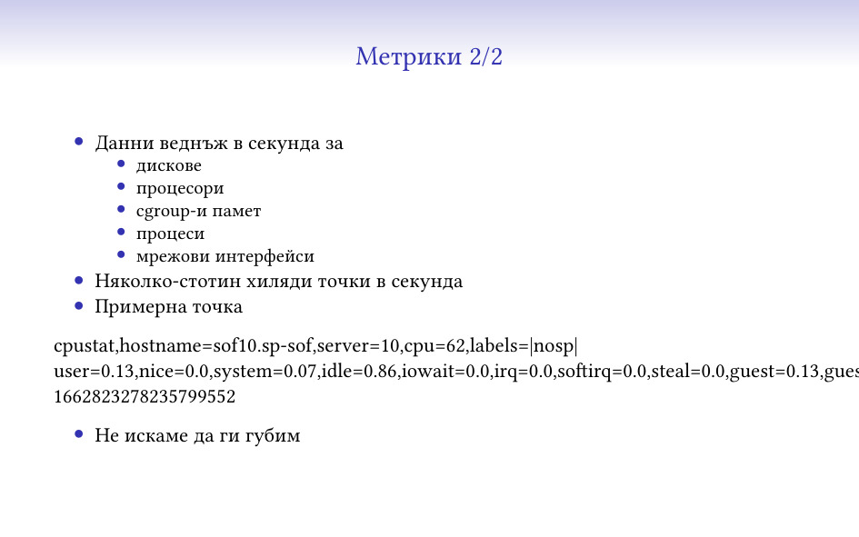
Метриките, които аз събирам са веднъж в секунда, за много различни компоненти
на системата – дискове, процесори, наши процеси, мрежови интерфейси. В момента
са няколко-стотин хиляди точки в секунда, и тук съм показал една примерна –
показва данните за една секунда за един процесор на една машина, заедно с малко
тагове (че например процесорът не се използва от storage системата, та за това
там пише “nosp”) и с timestamp.

Метриките са нещо, което не искаме да се изгуби по пътя или по някаква друга
причина, защото иначе може да се окаже, че не можем да разберем какво се е
случило в даден момент в системата. В някакъв вид те са като “логове”.

Метриките се събират веднъж в секунда, защото всичко друго не е достатъчно ясно
и може да изкриви информацията. Най-простия пример, който имам е как събитие,
което се случва веднъж в минута не може да бъде забелязано като отделно такова
на нищо, което не събира метрики поне веднъж на 10 секунди.

Също така, събития, които траят по секунда-две може да имат сериозно отражение
в/у потребителското усещане за работа на системата, което пак да трябва да е
нещо, което да трябва да се изследва. В 1-секундните метрики събитието може да
е се е “размазало” достатъчно, че да не е видимо и да е в границите на
статистическата грешка.

Имам любим пример, с cron, който работеше на една секунда и питаше един RAID
контролер “работи ли ти батерията?”. Това караше контролера да блокира всички
операции, докато провери и отговори, и на минутните графики имаше повишение на
латентността на операциите (примерно) от 200 на 270 микросекунди, и никой не
можеше да си обясни защо. На секундните си личеше, точно на началото на всяка
минута, един голям пик, който много бързо ни обясни какво става.

(отказвам да коментирам защо проверката на статуса на батерията или каквото и
да е, което питаме контролера отвисява нещата, най-вече защото не знам къде
живеят авторите на firmware)

Та това се налага да го обяснявам от време на време, и да се дразня на системи
като Prometheus, където практически по-добра от 3-секундна резолюция не може да
се постигне.

Също така, не знам дали мога да обясня колко е готино да пускате тестове, да
сте оставили една grafana да refresh-ва веднъж в секунда и почти в реално време
да може да виждате и да показвате на хората как влияят (или не) разлини
действия на системата, от типа на “тук заклахме половината мрежа и почти не се
усети”.

Другото нещо, което се следи е текущото състояние на системата. Това е нещото,
от което се смята статуса на системата в nagios, icinga и други, и от което се
казва “тук това не работи”. Системите, които получават тази информация решават
какви проблеми има, кого и дали да известят и всякакви такива неща.

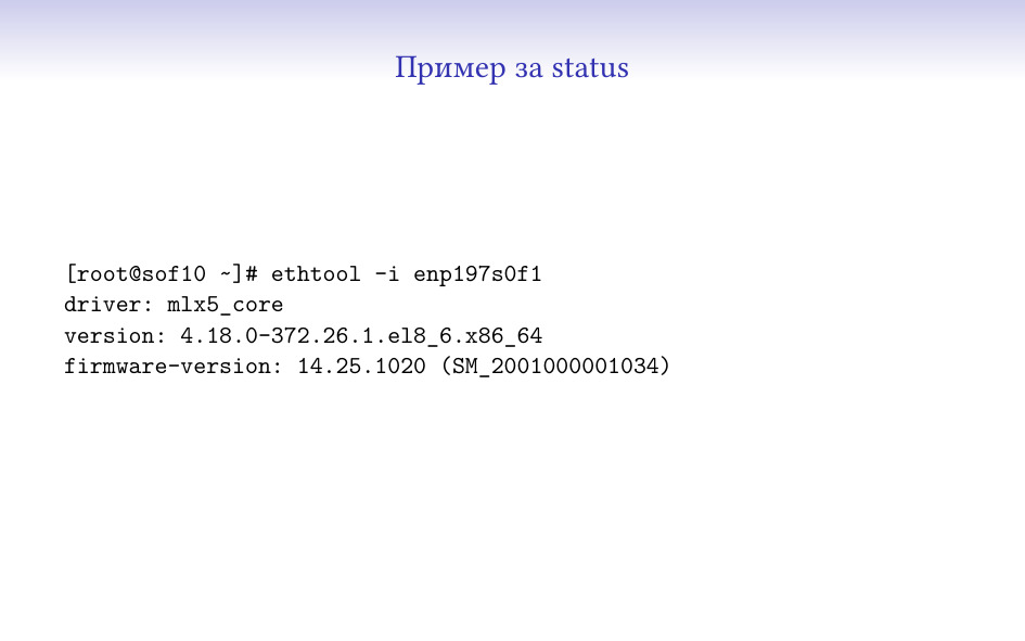
Статусът е нещо по-общо, и май нямам пример, който мога да събера на един слайд
и да може да се разбере нещо. Много често той носи допълнителна информация,
от която може да дойде нещо друго, например “мрежовата карта е с еди-коя-си
версия на firmware”, от което да решим, че там има известен проблем и да
показваме алармата по различен начин.

Метриките са доста по-ясни като формат, вид и употреба – имат измерение във
времето и ясни, числови параметри. Останалите данни рядко са толкова прости и
през повечето време съдържат много повече и различна информация, която не
винаги може да се представи по този начин.

Един пример, който мога да дам и който ми отне някакво време за писане беше
нещо, което разпознава дали дадени интерфейси са свързани на правилните места.
За целта събирах LLDP от всички сървъри, и после проверявах дали всички са
свързани по същия начин към същите switch-ове. Този тип информация сигурно може
да се направи във вид на метрики, но единствено ще стане по-труден за употреба,
вместо да има някаква полза.

А какъв е проблема с цялата тази работа, не е ли отдавна решен, може да се питате…

Като за начало, ако не се постараете, данните ви няма да стигнат до вас. Без
буфериране в изпращащата страна, без използване на резервни пътища и други
такива, ще губите достатъчна част от изпращаните си данни, че да имате дупки в
покритието и неяснота какво се случва/се е случило.

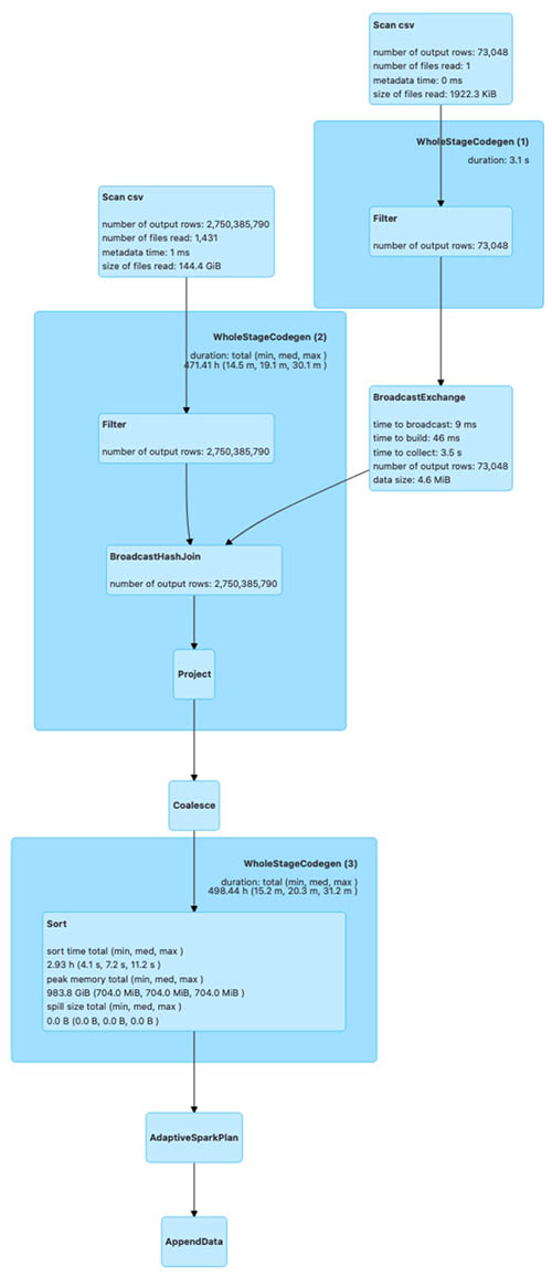
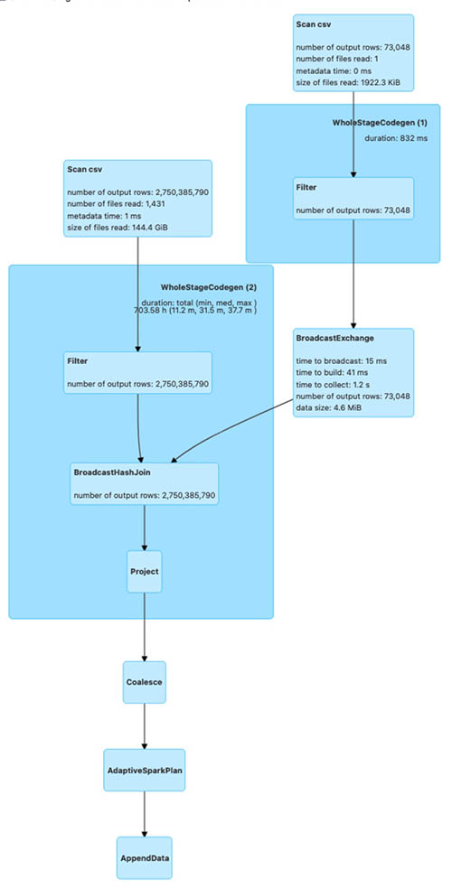
Данните са доста. Написал съм едни приблизителни числа, колкото да си проличи
генералния обем на данните, налагат се някакви трикове, така че да не ви удави,
и определено да имате достатъчно място и bandwidth за тях.

Дори като bandwidth не са малко, и хубавото на това, че имаме контрол в/у двете
страни, e че можем да си ги компресираме, и да смъкнем около 5 пъти трафика.
За това ни помага и че изпращаните данни са текстови, CSV или JSON – и двете
доста се поддават на компресия.

Няма някой друг service при нас, който да ползва сравнимо количество internet
bandwidth, дори някакви mirror-и 🙂

Идващите данни трябва да се съхраняват за някакво време. Добре, че фирмата
се занимава със storage, та ми е по-лесно да си поискам хардуер за целта…

За да можем все пак да съберем всичко, пазим само 2 дни секундни данни и 1
година минутни. InfluxDB се справя прилично добре да ги компресира – мисля, че
в момента пазим общо около двайсетина TB данни само за метрики. За
monitoring данните за debug цели държим пращаните от последните 10 часа, но
това като цяло е лесно разширимо, ако реша да му дам още място, за момента
се събират в около 1.6TiB.
(Това е и една от малкото ми употреби на btrfs, защото изглежда като
единствената достъпна файлова система с компресия… )

Ако погледнем още един път числата обаче, тук няма нищо толкова голямо, че да
не е постижимо в почти “домашни” условия. Гигабит интернет има откъде да си
намерите, терабайтите storage дори на ssd/nvme вече не са толкова
скъпи, и скорошните сървърни процесори на AMD/Intel като цяло могат да вършат
спокойно тая работа. Та това е към обясненията “всъщност, всеки може да си го
направи” 🙂

Системите, които наблюдаваме са дистрибутирани, shared-nothing, съответно
сравнително сложни и проверката дали нещо е проблем често включва “сметка” от
няколко парчета данни. Като сравнително прост пример за някаква базова проверка
– ако липсва даден диск, е проблем, но само ако не сме казали изрично да бъде
изваден (флаг при диска) или ако се използва (т.е. присъства в едни определени
списъци). Подобни неща в нормална monitoring система са сложни за описване и
биха изисквали език за целта.

Имаме и случаи, в които трябва да се прави някаква проверка на база няколко
различни системи, например такива, които регулярно си изпращат данни – дали
това, което едната страна очаква, го има от другата. Понякога отсрещните страни
може да са няколко 🙂

Статусът се изпраща веднъж в минута, и е добре да може да се обработи
достатъчно бързо, че да не се натрупва опашка от статуси на същата система.
Това значи, че monitoring-ът някакси трябва да успява да сдъвче данните
достатъчно бързо и да даде резултат, който да бъде гледан от хора.

Това има значение и за колко бързо успяваме да реагираме на проблеми, защото
все пак да се реагира трябва трябва да има на какво 🙂

И имаме нужда тази система да е една и централизирана, за можем да следим
стотиците системи на едно място. Да гледаш 100 различни места е много трудно и
на практика загубена кауза. Да не говорим колко трудно се оправдава да се сложи
по една система при всеки deployment само за тази цел.

Това има и други предимства, че ако наблюдаваните системи просто изпращат данни
и ние централно ги дъвчем, промяна в логиката и добавяне на нов вид проверка
става много по-лесно. Дори в модерните времена, в които deployment-а на хиляда
машини може да е сравнително бърз, пак трудно може да се сравнява с един локален
update.

И това трябва да работи, защото без него сме слепи и не знаем какво се случва,
не го знаят и клиентите ни, които ползват нашия monitoring. Усещането е като
донякъде да стоиш в тъмна стая и да чакаш да те ударят по главата…

От какво е сглобена текущата ни система?

За база на системата използвам icinga2. В нея се наливат конфигурации, статуси
и тя решава какви аларми да прати и поддържа статус какво е състоянието в
момента.

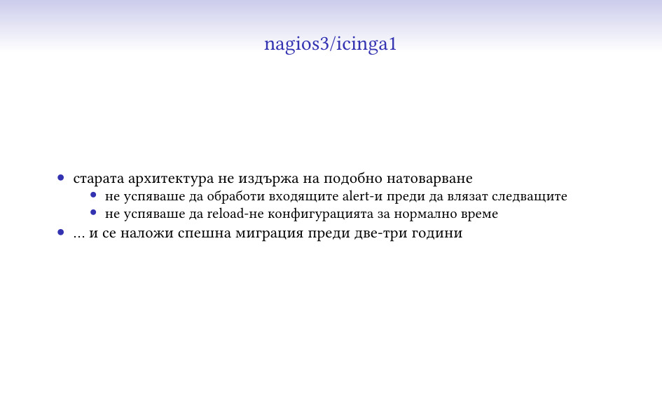
Беше upgrade-ната от icinga1, която на около 40% от текущото натоварване умря и
се наложи спешна миграция.

InfluxDB, по времето, в което започвах да пиша системата беше най-свястната от
всичките съществуващи time series бази.

Като изключим доста осакатения език за заявки (който се прави на SQL, но е
много далеч и е пълен със странни ограничения), и че не трябва да се приема за
истинска база (много глезотии на mysql/pgsql ги няма), InfluxDB се справя добре
в последните си версии и не може да бъде crash-ната с някоя заявка от
документацията. Основното нещо, което ми се наложи да правя беше да прескоча
вътрешния механизъм за агрегиране на данни и да си напиша мой (който не помня
дали release-нахме), който да може да върши същото нещо паралелно и с още малко
логика, която ми трябваше.

От някакво време има и версия 2, която обаче е променила достатъчно неща, че да
не мога още да планирам миграция до нея.

Както обясних, проверките по принцип са не-елементарни (трудно ми е да кажа
сложни) и логиката за тях е изнесена извън icinga.

В момента има около 10k реда код, понеже се добавиха всякакви глезотии и
интересни функционалности (човек като има много данни, все им намира
приложение), но началната версия за базови неща беше около 600 реда код, с
всичко базово. Не мисля, че отне повече от няколко дни да се сглоби и да се
види, че може да върши работа.


Ако ползвате стандартен метод за активни проверки (нещо да се свързва до
отсрещната страна, да задава въпрос и от това да дава резултат), никога няма да
стигнете хиляди в секунда без сериозно клъстериране и ползване много повече
ресурси.

Дори и да не ползвате стандартните методи, пак по-старите версии на icinga не
се справят с толкова натоварване. При нас преди няколко години надминахме
лимита на icinga1 и изборът беше м/у миграция или клъстериране. Миграцията се
оказа по-лесна (и даде някакви нови хубави функционалност, да не говорим, че се
ползваше вече софтуер от тоя век).

Основният проблем е архитектурен, старата icinga е един процес, който прави
всичко и се бави на всякакви неща, като комуникация с други процеси,
писане/четене от диска, и колкото и бърза да ни е системата, просто не може да
навакса при около 20-30к съществуващи услуги и няколко-стотин статуса в
секунда. А като му дадеш да reload-не конфигурацията, и съвсем клякаше.

Изобщо, технически това един бивш колега го описваше като “десет литра лайна
в пет литра кофа”.

Новата например reload-ва в отделен процес, който не пречи на главния.

Признавам си, не обичам Prometheus. Работи само на pull, т.е. трябва да може да
се свързва до всичките си крайни станции, и като го пуснахме за вътрешни цели с
около 100-200 машини, почна да му става сравнително тежко при проверка на 3
секунди. Също така изобщо няма идеята да се справя с проблеми на internet-а,
като просто интерполира какво се е случило в периода, в който не е имал
свързаност.

Върши работа за някакви неща, но определен е далеч от нашия случай. Според мен
е и далеч от реалността и единствената причина да се ползва толкова е многото
натрупани готови неща под формата на grafana dashboard-и и exporter-и.


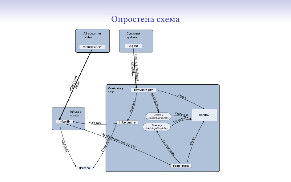
Компонентите са в общи лини ясни:

Агентите събират информация и се стараят да ни я пратят;

Получателите я взимат, анализират, записват и т.н.;

Анализаторите дъвчат събраната информация и на база на нея добавят още
проверки.

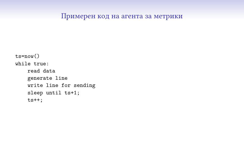
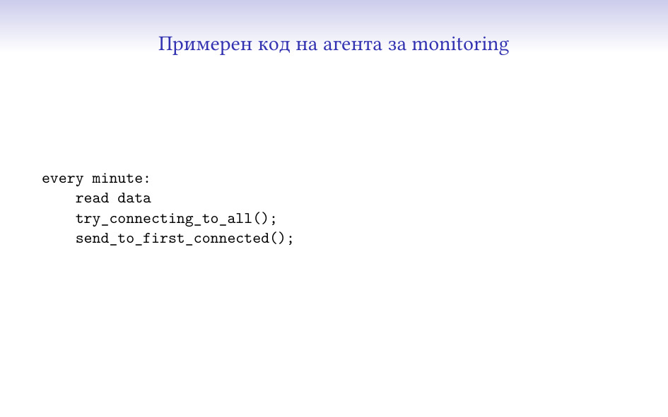
Тук не измислих как да го покажа, но това е един thread, който събира данни (от
няколко такива), и има един който изпраща данните и се старае да стигнат. Пак е
сравнително малко код и може да бъде сглобен почти от всеки.

За данни, за които повече бързаме да получим и не буферираме, има друг
интересен трик – да имате няколко входни точки (при нас освен нашия си интернет
имаме един “домашен”, който да работи дори да стане някакво бедствие с
останалия), съответно агентът се опитва да се свърже едновременно с няколко
места и което първо отговори, получава данните.

Понеже това е писано на perl по исторически причини, беше малко странно да се
направи (понеже select/poll на perl, non-blocking връзки и подобни неща не са
съвсем стандартни), но сега мога да го похваля, че работи много добре и се
справя вкл. и с IPv6 свързаност.

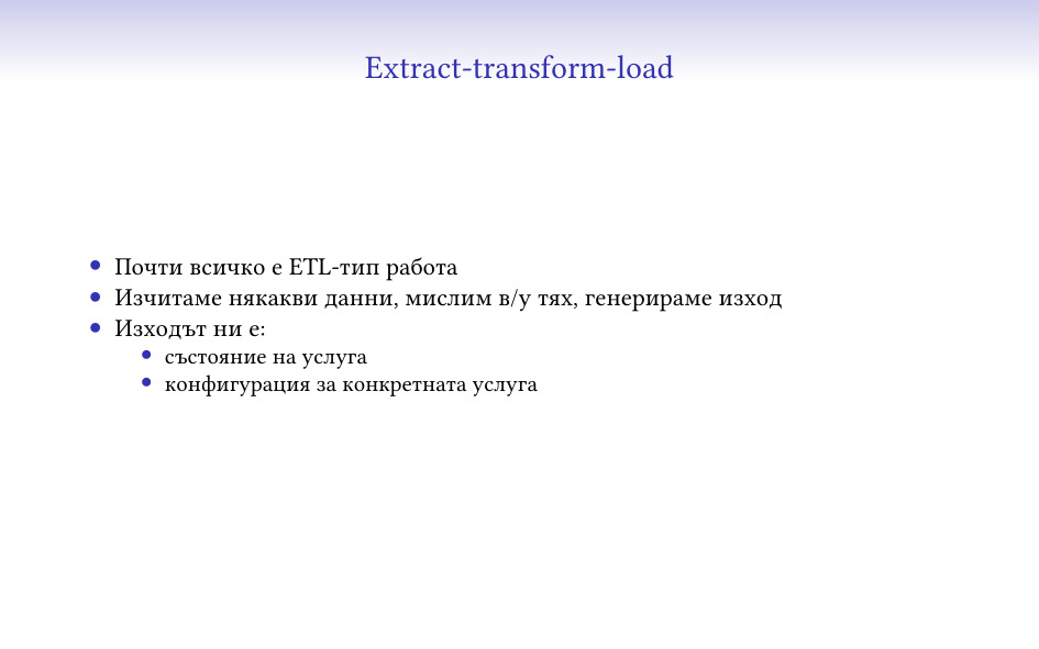
И всичкия код, който получава/прави анализи си е тип ETL
(extract-transform-load). Взима едни данни, дъвче, качва обратно.

В нашия случай това, което връща са състояния и конфигурации (ще го покажа
по-долу).

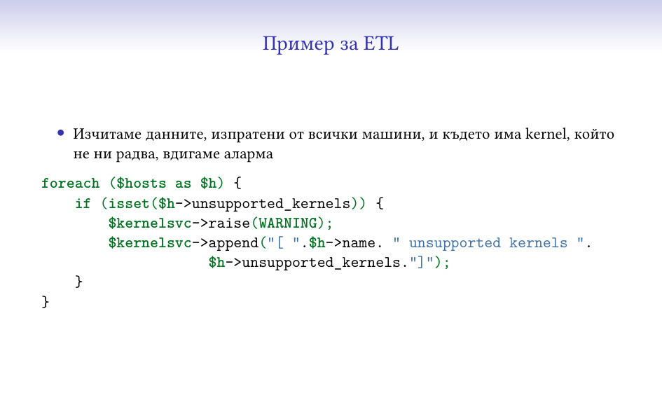
И един елементарен пример, почти директно от кода – обикаля данните за набор от
машини, проверява дали в тях има нещо определено (kernel, за който нямаме
качена поддръжка) и го отбелязва.

Има и по-интересни такива неща (анализи на латентности от метриките, например),
но нямаше да са добър пример за тук 🙂

“Липсата на сигнал е сигнал” – можем да знаем, че нещо цялостно или част от
него не ни говори, понеже имаме контрол в/у агентите и кода им, и знаем
кога/как трябва да се държат.

Някой би казал, че това се постига по-добре с активна проверка (“тия хора
пингват ли се?”), но това се оказва много сложно да се прави надеждно, през
интернета и хилядите firewall-и по пътя. Също така, не може да се очаква
интернета на всички да работи добре през цялото време (заради което и всичките
агенти са направени да се борят с това).

Както казах по-рано, Интернета не работи 🙂

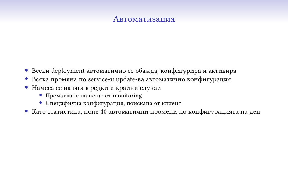
Един от най-важните моменти в подобна система е колко работа изисква за
рутинните си операции. Понеже аз съм мързел и не обичам да се занимавам с
описване на всяка промяна, системата автоматично се конфигурира на база на
пристигналите данни, решава какви системи следи, какви услуги, вижда дали нещо
е изчезнало и т.н. и като цяло работи съвсем сама без нужда от пипане.

Има функционалност за специфична конфигурация за клиент, която изисква ръчна
намеса, както и изтриването на цялостни системи от monitoring-а, но това като
цяло са доста редки случаи.

Системата се грижи всичко останало да се случва съвсем само.

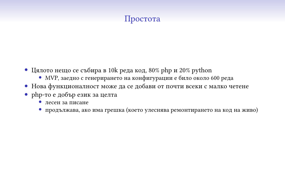
Това, което според мен е най-важното за тази и подобни системи – няма нищо
особено сложно в тях, и всеки, който се нуждае от нещо такова може да си го
сглоби. Първоначалната ми версия е била около 600 реда код, и дори в момента в
10-те хиляди реда човек може да се ориентира сравнително лесно и да добави
нещо, ако му се наложи.

Като пример, дори python програмистите при нас, които считат, че php-то трябва
да се забрани със закон, са успявали да си добавят функционалност там
сравнително лесно и със съвсем малко корекции по стила от моя страна.

Самото php се оказва много удобно за подобни цели, основно защото успява да се
справи и с объркани данни (което се случва при разни ситуации) и не убива
всичко, а си се оплаква и свършва повечето работа. Разбира се, това не е
единствения подходящ език, аз лично писах на него, защото ми беше лесен – но
ако искате да сглобите нещо, в наши дни може да го направите почти на каквото и
си искате и да работи. Python и js са някакви основни кандидати (като езици,
дето хората знаят по принцип), само не препоръчвам shell и C 🙂

Така че, ако ви трябва нещо такова – с по-сложна логика, да издържа повече
натоварване, да прави неща, дето ги няма в други системи – не е особено сложно
да го сглобите и да тръгне, нещо минимално се сглабя за няколко дни, а се
изплаща супер бързо 🙂

Monitoring системата се налага да се следи, разбира се. Всичкият софтуер се
чупи, този, който аз съм правил – още повече. По случая други колеги направиха
нещо, което да следи всичките ни вътрешни физически и виртуални машини, и това
между другото следи и големия monitoring 🙂

Изглежда по коренно различен начин – използва Prometheus, Alertmanager и за
база VictoriaMetrics, което в общи линии значи, че двете системи рядко имат
същите видове проблеми. Също така и допълнителния опит с Prometheus ми показа,
че определено е не е бил верния избор за другата система 🙂

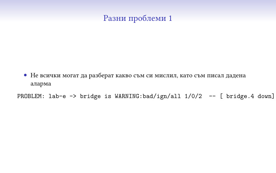
Може би най-големият проблем, който съм имал е да обясня какво значи текста на
дадена аларма на други колеги. Тук например съм казал “има малък проблем (за
това е WARNING), в услугата bridge, има един счупен, нула игнорирани (по разни
причини) и 2 общо, и този на машина 4 е down” – и това поне трима различни
човека са ми казвали, че не се разбира. Последното ми решение на проблема е да
карам да ми дадат как очакват да изглежда и да го пренаписвам. От една страна,
съобщенията станаха по-дълги, от друга – не само аз ги разбирам 🙂

Няколко пъти се е случвало системата да изпрати notification на много хора по
различни причини – или грешка в някоя аларма, или просто има проблем на много
места. Като цяло първото може доста да стресне хората, съответно вече (със
съвсем малко принуда) има няколко staging среди, които получават всички
production данни и в които може да се види какво ще светне, преди да е стигнало
до хора, които трябва да му обръщат внимание.

Изобщо, ако човек може да си го позволи, най-доброто тестване е с production
данните.

Основна задача за всяка такава система трябва да е да се намалят алармите до
минимум. Би трябвало фалшивите да са минимален брой (ако може нула), а едно
събитие да генерира малко и информативни такива. Също така, трябва да има лесен
механизъм за “умълчаване” на някаква част от алармите, когато нещо е очаквано.

Това е може би най-сложната задача, понеже да се прецени кога нещо е проблем и
кога не е изисква анализ и познаване на системата, понякога в дълбини, в които
никой не е навлизал.

Решението тук е да се вземат алармите за един ден, и да се види кое от тях е
безсмислено и кое може да се махне за сметка на нещо друго, след което мноооого
внимателно да се провери, че това няма да скрие истински проблем, вероятно с
гледане на всички останали задействания на неприемливото съобщение. Което е
бавна, неблагодарна и тежка работа 🙂

Не исках да слагам този slide в началото, че сигурно нямаше да остане никой да
слуша лекцията. Оставям го да говори сам за себе си:)

The collective thoughts of the interwebz