The kernel’s Bugzilla
instance is largely unloved and ignored, at least as a bug-reporting
tool for the bulk of the upstream kernel. At the recent Maintainers Summit,
Bugzilla was discussed during the regression-handling session led by Thorsten
Leemhuis. In a followup to that discussion, Leemhuis posted
some ideas for improving the state of bugzilla.kernel.org to the
ksummit-discuss mailing list recently; the resulting discussion helped
clarify a number of problem areas for it—and for the Bugzilla tool itself.
“Никой няма да забрави картините с пороя, удавил на втори септември трите карловски села – Каравелово, Богдан и Слатина. И трите са в подножието на планината – Средна гора. Истински…
In modern data architectures, it’s common to store data in multiple data sources. However, organizations embracing this approach still need insights from their data and require technologies that help them break down data silos. Amazon Athena is an interactive query service that makes it easy to analyze structured, unstructured, and semi-structured data stored in Amazon Simple Storage Service (Amazon S3) in addition to relational, non-relation, object, and custom data sources through its query federation capabilities. Athena is serverless, so there’s no infrastructure to manage, and you only pay for the queries that you run.
Organizations building a modern data architecture want to query data in-place from purpose-built data stores without building complex extract, transform, and load (ETL) pipelines. Athena’s federated query feature allows organizations to achieve this and makes it easy to:
Create reports and dashboards from data stored in relational, non-relational, object, and custom data sources
Run on-demand analysis on data spread across multiple systems of record using a single tool and single SQL dialect
Join multiple data sources together to produce new input features for machine learning model training workflows
However, when querying and joining huge amounts of data from different data stores, it’s important for queries to run quickly, at low cost, and without impacting source systems. Predicate pushdown is supported by many query engines and is a technique that can drastically reduce query processing time by filtering data at the source early in the processing workflow. In this post, you’ll learn how predicate pushdown improves query performance and how you can validate when Athena applies predicate pushdown to federated queries.
Benefits of predicate pushdown
The key benefits of predicate pushdown are as follows:
Improved query runtime
Reduced network traffic between Athena and the data source
Reduced load on the remote data source
Reduced cost resulting from reduced data scans
Let’s explore a real-world scenario to understand when predicate pushdown is applied to federated queries in Athena.
Solution overview
Imagine a hypothetical ecommerce company with data stored in
Amazon Redshift – Company’s Datawarehouse, used for current and historical analytics
Amazon DynamoDB – NoSQL Database, used for real-time inventory tracking and latest supplier data in the company
Record counts for these tables are as follows.
Data Store
Table Name
Number of Records
Description
Amazon Redshift
Catalog_Sales
4.3 billion
Current and historical Sales data fact Table
Amazon Redshift
Date_dim
73,000
Date Dimension table
DynamoDB
Part
20,000
Realtime Parts and Inventory data
DynamoDB
Partsupp
80,000
Realtime Parts and supplier data
Aurora MySQL
Supplier
1,000
Latest Supplier transactions
Aurora MySQL
Customer
15,000
Latest Customer transactions
Our requirement is to query these sources individually and join the data to track pricing and supplier information and compare recent data with historical data using SQL queries with various filters applied. We’ll use Athena federated queries to query and join data from these sources to meet this requirement.
The following diagram depicts how Athena federated queries use data source connectors run as Lambda functions to query data stored in sources other than Amazon S3.
When a federated query is submitted against a data source, Athena invokes the data source connector to determine how to read the requested table and identify filter predicates in the WHERE clause of the query that can be pushed down to the source. Applicable filters are automatically pushed down by Athena and have the effect of omitting unnecessary rows early in the query processing workflow and improving overall query execution time.
Let’s explore three use cases to demonstrate predicate pushdown for our ecommerce company using each of these services.
Prerequisites
As a prerequisite, review Using Amazon Athena Federated Query to know more about Athena federated queries and how to deploy these data source connectors.
Use case 1: Amazon Redshift
In our first scenario, we run an Athena federated query on Amazon Redshift by joining its Catalog_sales and Date_dim tables. We do this to show the number of sales orders grouped by order date. The following query gets the information required and takes approximately 14 seconds scanning approximately 43 MB of data:
SELECT "d_date" AS Order_date,
     count(1) AS Total_Orders
 FROM "lambda:redshift"."order_schema"."catalog_sales" l,
     "lambda:redshift"."order_schema"."date_dim" d
 WHERE l.cs_sold_date_sk = d_date_sk
     and cs_sold_date_sk between 2450815 and 2450822 --Date keys for first week of Jan 1998
 GROUP BY "d_date"
 order by "d_date"
Athena pushes the following filters to the source for processing:
cs_sold_date_sk between 2450815 and 2450822 for the Catalog_Sales table in Amazon Redshift.
d_date_sk between 2450815 and 2450822; because of the join l.cs_sold_date_sk=d_date_sk in the query, the Date_dim table is also filtered at the source, and only filtered data is moved from Amazon Redshift to Athena.
Let’s analyze the query plan by using recently released visual explain tool to confirm the filter predicates are pushed to the data source:
As shown above (only displaying the relevant part of the visual explain plan), because of the predicate pushdown, the Catalog_sales and Date_dim tables have filters applied at the source. Athena processes only the resulting filtered data.
Using the Athena console, we can see query processing details using the recently released query stats to interactively explore processing details with predicate pushdown at the query stage:
Displaying only the relevant query processing stages, Catalog_sales table has approximately 4.3 billion records, and Date_dim has approximately 73,000 records in Amazon Redshift. Only 11 million records from the Catalog_sales (Stage 4) and 8 records from the Date_dim (Stage 5) are passed from source to Athena, because the predicate pushdown pushes query filter conditions to the data sources. This filters out unneeded records at the source, and only brings the required rows to Athena.
Using predicate pushdown resulted in scanning 99.75% less data from Catalog_sales and 99.99% less data from Date_dim. This results in a faster query runtime and lower cost.
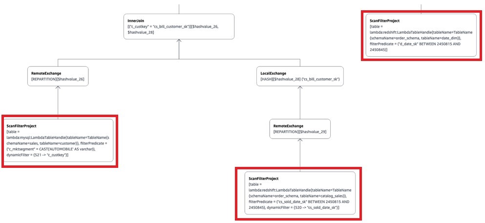
Use case 2: Amazon Redshift and Aurora MySQL
In our second use case, we run an Athena federated query on Aurora MySQL and Amazon Redshift data stores. This query joins the Catalog_sales and Date_dim tables in Amazon Redshift with the Customer table in the Aurora MySQL database to get the total number of orders with the total amount spent by each customer for the first week in January 1998 for the market segment of AUTOMOBILE. The following query gets the information required and takes approximately 35 seconds scanning approximately 337 MB of data:
SELECT  cs_bill_customer_sk Customer_id ,"d_date" Order_Date
 ,count("cs_order_number") Total_Orders ,sum(l.cs_net_paid_inc_ship_tax) AS Total_Amount
 FROM "lambda:mysql".sales.customer c,"lambda:redshift"."order_schema"."catalog_sales" l
 ,"lambda:redshift"."order_schema"."date_dim" d
 WHERE c_mktsegment = 'AUTOMOBILE'
 AND c_custkey = cs_bill_customer_sk
 AND l.cs_sold_date_sk=d_date_sk
 AND cs_sold_date_sk between 2450815 and 2450822 --Date keys for first week of Jan 1998
 GROUP BY cs_bill_customer_sk,"d_date"
 ORDER BY cs_bill_customer_sk,"d_date"
Athena pushes the following filters to the data sources for processing:
cs_sold_date_sk between 2450815 and 2450822 for the Catalog_Sales table in Amazon Redshift.
d_date_sk between 2450815 and 2450822; because of the join l.cs_sold_date_sk=d_date_sk in the query, the Date_dim table is also filtered at the source (Amazon Redshift) and only filtered data is moved from Amazon Redshift to Athena.
c_mktsegment = 'AUTOMOBILE' for the Customer table in the Aurora MySQL database.
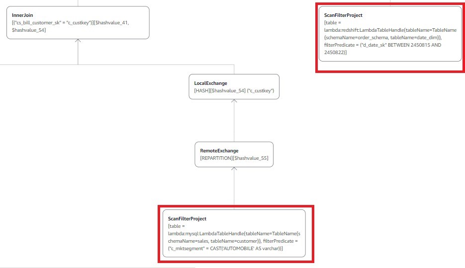
Now let’s consult the visual explain plan for this query to show the predicate pushdown to the source for processing:
As shown above (only displaying the relevant part of the visual explain plan), because of the predicate pushdown, Catalog_sales and Date_dim have the query filter applied at the source (Amazon Redshift), and the customer table has the market segment AUTOMOBILE filter applied at the source (Aurora MySQL). This brings only the filtered data to Athena.
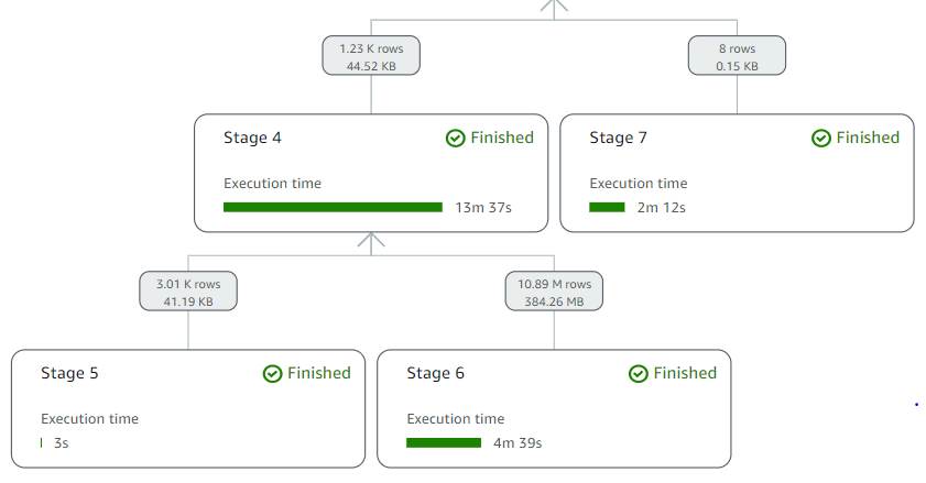
As before, we can see query processing details using the recently released query stats to interactively explore processing details with predicate pushdown at the query stage:
Displaying only the relevant query processing stages, Catalog_sales has 4.3 billion records, Date_Dim has 73,000 records in Amazon Redshift, and Customer has 15,000 records in Aurora MySQL. Only 11 million records from Catalog_sales (Stage 6), 8 records from Date_dim (Stage 7), and 3,000 records from Customer (Stage 5) are passed from the respective sources to Athena because the predicate pushdown pushes query filter conditions to the data sources. This filters out unneeded records at the source and only brings the required rows to Athena.
Here, predicate pushdown resulted in scanning 99.75% less data from Catalog_sales, 99.99% less data from Date_dim, and 79.91% from Customer. Furthermore, this results in a faster query runtime and reduced cost.
Use case 3: Amazon Redshift, Aurora MySQL, and DynamoDB
For our third use case, we run an Athena federated query on Aurora MySQL, Amazon Redshift, and DynamoDB data stores. This query joins the Part and Partsupp tables in DynamoDB, the Catalog_sales and Date_dim tables in Amazon Redshift, and the Supplier and Customer tables in Aurora MySQL to get the quantities available at each supplier for orders with the highest revenue during the first week of January 1998 for the market segment of AUTOMOBILE and parts manufactured by Manufacturer#1.
The following query gets the information required and takes approximately 33 seconds scanning approximately 428 MB of data in Athena:
SELECT "d_date" Order_Date
     ,c_mktsegment
     ,"cs_order_number"
     ,l.cs_item_sk Part_Key
     ,p.p_name Part_Name
     ,s.s_name Supplier_Name
     ,ps.ps_availqty Supplier_Avail_Qty
     ,l.cs_quantity Order_Qty
     ,l.cs_net_paid_inc_ship_tax Order_Total
 FROM "lambda:dynamo".default.part p,
     "lambda:mysql".sales.supplier s,
     "lambda:redshift"."order_schema"."catalog_sales" l,
     "lambda:dynamo".default.partsupp ps,
     "lambda:mysql".sales.customer c,
     "lambda:redshift"."order_schema"."date_dim" d
 WHERE
     c_custkey = cs_bill_customer_sk
     AND l.cs_sold_date_sk=d_date_sk
     AND c.c_mktsegment = 'AUTOMOBILE'
     AND cs_sold_date_sk between 2450815 and 2450822 --Date keys for first week of Jan 1998
     AND p.p_partkey=ps.ps_partkey
     AND s.s_suppkey=ps.ps_suppkey
     AND p.p_partkey=l.cs_item_sk
     AND p.p_mfgr='Manufacturer#1'
Athena pushes the following filters to the data sources for processing:
cs_sold_date_sk between 2450815 and 2450822 for the Catalog_Sales table in Amazon Redshift.
d_date_sk between 2450815 and 2450822; because of the join l.cs_sold_date_sk=d_date_sk in the query, the Date_dim table is also filtered at the source and only filtered data is moved from Amazon Redshift to Athena.
c_mktsegment = 'AUTOMOBILE' for the Customer table in the Aurora MySQL database.
p.p_mfgr='Manufacturer#1' for the Part table in DynamoDB.
Now let’s run the explain plan for this query to confirm predicates are pushed down to the source for processing:
As shown above (displaying only the relevant part of the plan), because of the predicate pushdown, Catalog_sales and Date_dim have the query filter applied at the source (Amazon Redshift), the Customer table has the market segment AUTOMOBILE filter applied at the source (Aurora MySQL), and the Part table has the part manufactured by Manufacturer#1 filter applied at the source (DynamoDB).
We can analyze query processing details using the recently released query stats to interactively explore processing details with predicate pushdown at the query stage:
Displaying only the relevant processing stages, Catalog_sales has 4.3 billion records, Date_Dim has 73,000 records in Amazon Redshift, Customer has 15,000 records in Aurora MySQL, and Part has 20,000 records in DynamoDB. Only 11 million records from Catalog_sales (Stage 5), 8 records from Date_dim (Stage 9), 3,000 records from Customer (Stage 8), and 4,000 records from Part (Stage 4) are passed from their respective sources to Athena, because the predicate pushdown pushes query filter conditions to the data sources. This filters out unneeded records at the source, and only brings the required rows from the sources to Athena.
Considerations for predicate pushdown
When using Athena to query your data sources, consider the following:
Depending on the data source, data source connector, and query complexity, Athena can push filter predicates to the source for processing. The following are some of the sources Athena supports predicate pushdown with:
Athena also performs predicate pushdown on data stored in an S3 data lake. And, with predicate pushdown for supported sources, you can join all your data sources in one query and achieve fast query performance.
You can use the recently released query stats as well as EXPLAIN and EXPLAIN ANALYZE on your queries to confirm predicates are pushed down to the source.
Queries may not have predicates pushed to the source if the query’s WHERE clause uses Athena-specific functions (for example, WHERE log2(col)<10).
Conclusion
In this post, we demonstrated three federated query scenarios on Aurora MySQL, Amazon Redshift, and DynamoDB to show how predicate pushdown improves federated query performance and reduces cost and how you can validate when predicate pushdown occurs. If the federated data source supports parallel scans, then predicate pushdown makes it possible to achieve performance that is close to the performance of Athena queries on data stored in Amazon S3. You can utilize the patterns and recommendations outlined in this post when querying supported data sources to improve overall query performance and minimize data scanned.
About the authors
Rohit Bansal is an Analytics Specialist Solutions Architect at AWS. He has nearly two decades of experience helping customers modernize their data platforms. He is passionate about helping customers build scalable, cost-effective data and analytics solutions in the cloud. In his spare time, he enjoys spending time with his family, travel, and road cycling.
Ruchir Tripathi is a Senior Analytics Solutions Architect aligned to Global Financial Services at AWS. He is passionate about helping enterprises build scalable, performant, and cost-effective solutions in the cloud. Prior to joining AWS, Ruchir worked with major financial institutions and is based out of New York Office.
To build a data lake on AWS, a common data ingestion pattern is to use AWS Glue jobs to perform extract, transform, and load (ETL) data from relational databases to Amazon Simple Storage Service (Amazon S3). A project often involves extracting hundreds of tables from source databases to the data lake raw layer. And for each source table, it’s recommended to have a separate AWS Glue job to simplify operations, state management, and error handling. This approach works perfectly with a small number of tables. However, with hundreds of tables, this results in hundreds of ETL jobs, and managing AWS Glue jobs at this scale may pose an operational challenge if you’re not yet ready to deploy using a CI/CD pipeline. Instead, we tackle this issue by decoupling the following:
ETL job logic – We use an AWS Glue blueprint, which allows you to reuse one blueprint for all jobs with the same logic
Job definition – We use a JSON file, so you can define jobs programmatically without learning a new language
Job deployment – With AWS Step Functions, you can copy workflows to manage different data processing use cases on AWS Glue
In this post, you will learn how to handle data lake landing jobs deployment in a standardized way—by maintaining a JSON file with table names and a few parameters (for example, a workflow catalog). AWS Glue workflows are created and updated after manually running the resources deployment flow in Step Functions. You can further customize the AWS Glue blueprints to make your own multi-step data pipelines to move data to downstream layers and purpose-built analytics services (example use cases include partitioning or importing to an Amazon DynamoDB table).
Overview of solution
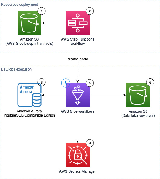
The following diagram illustrates the solution architecture, which contains two major areas:
Resource deployment (components 1–2) – An AWS Step Functions workflow is run manually on demand to update or deploy the required AWS Glue resources. These AWS Glue resources will be used for landing data into the data lake
ETL job runs (components 3–6) – The AWS Glue workflows (one per source table) run on the defined schedule, and extract and land data to the data lake raw layer
The solution workflow contains the following steps:
An S3 bucket stores an AWS Glue blueprint (ZIP) and the workflow catalog (JSON file).
A Step Functions workflow orchestrates the AWS Glue resources creation.
We use Amazon Aurora as the data source with our sample data, but any PostgreSQL database works with the provided script, or other JDBC sources with customization.
If you want to use your existing database either in AWS or on premises as a data source, you need network connectivity (a subnet and security group) for the AWS Glue jobs that can access the source database, Amazon S3, and Secrets Manager.
Provision resources with AWS CloudFormation
In this step, we provision our solution resources with AWS CloudFormation.
Database with sample data (optional)
This CloudFormation stack works only in AWS Regions where Amazon Aurora Serverless v1 is supported. Complete the following steps to create a database with sample data:
Choose Launch Stack.
On the Create stack page, choose Next.
For Stack name, enter demo-database.
For DBSecurityGroup, choose select the security group for the database (for example, default).
For DBSubnet, choose two or more private subnets to host the database.
For ETLAZ, choose the Availability Zone for ETL jobs. It must match with ETLSubnet.
For ETLSubnet, choose the subnet for the jobs. This must match with ETLAZ.
To find the subnet and corresponding Availability Zone, go to the Amazon Virtual Private Cloud (Amazon VPC) console and look at the columns Subnet ID and Availability Zone.
Choose Next.
On the Configure stack options page, skip the inputs and choose Next.
On the Review page, choose Create stack.
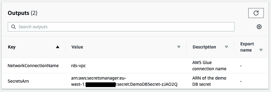
When the stack is complete, go to the Outputs tab and note the value for SecretsARN.
This CloudFormation stack creates the following resources:
In the Connect to database section, provide the following information:
For Database instance, enter demo-<123456789012>.
For Database username, connect with a Secrets Manager ARN.
For Secrets Manager ARN, enter the ARN from the outputs of the CloudFormation stack.
For Database name, enter hr.
Choose Connect to database.
Enter the contents of the SQL file into the editor, then choose Run.
Main stack (required)
This CloudFormation stack works in all AWS Regions.
Choose Launch Stack.
On the Create stack page, choose Next.
For Stack name, enter data-lake-landing.
For BlueprintName, enter a name for your blueprint (default: data-lake-landing).
For S3BucketNamePrefix, enter a prefix (default: data-lake-raw-layer).
Choose Next.
On the Configure stack options page, skip the inputs and choose Next.
On the Review page, select I acknowledge that AWS CloudFormation might create IAM resources with custom names.
Choose Create stack.
When the stack is complete, go to the Outputs tab and note the names of the S3 bucket (for example, data-lake-raw-layer-123456789012-region) and Step Functions workflow (for example, data-lake-landing).
The CloudFormation stack creates the following resources:
An S3 bucket as the data lake raw layer
A Step Functions workflow (see the definition on the GitHub repo)
AWS Identity and Access Management (IAM) roles and policies for the Step Functions workflow to provision AWS Glue resources and AWS Glue job executions.
The GlueExecutionRole is limited to the DemoDBSecret in Secrets Manager. If you need to connect to other databases which has a different endpoint/address or credentials, don’t forget to create new secrets and grant additional permissions to the IAM role or secrets so your AWS Glue jobs can authenticate with the source databases.
Prepare database connections
If you want to use this solution to perform ETL against your existing databases, follow this section. Otherwise, if you have deployed the CloudFormation stack for the database with sample data, jump to the section “Edit the workflow catalog”.
You need to have a running PostgreSQL database ready. To connect to other database engines, you need to customize this solution, particularly the jdbcUrl in the supplied PySpark script.
Create the database secret
To create your Secrets Manager secret, complete the following steps:
For the VPC, subnet, and security groups (prepared in the prerequisite steps), enter where the ETL jobs run and are able to connect to the source database, Amazon S3, and Secrets Manager.
Choose Create connection.
You’re now ready to configure the rest of the solution.
Edit the workflow catalog
To download the workflow catalog, complete the following steps:
If you are using the provided sample database, you must change the values of GlueExecutionRole and DestinationBucketName. If you are using your own databases, you must change all vaules except WorkflowName, JobScheduleType, and ScheduleCronPattern.
Rename the file your_blueprint_name.json and upload it to your S3 bucket (for example, s3://data-lake-raw-layer-123456789012-eu-west-1/data-lake-landing.json).
The example workflow has the JobScheduleType set to Cron. See Time-based schedules for jobs and crawlers for examples setting cron patterns. Alternatively set JobScheduleType to OnDemand.
Write the DataFrame to Amazon S3 as Parquet files.
Prepare the AWS Glue blueprint
Prepare your AWS Glue blueprint with the following steps:
Download the sample file and unzip it in your local computer.
Make any necessary changes to the PySpark script to include your own logic, and compress the three files (blueprint.cfg, jdbc_to_s3.py, layout.py; exclude any folders) as your_blueprint_name.zip (for example, data-lake-landing.zip):
zip data-lake-landing.zip blueprint.cfg jdbc_to_s3.py layout.py
Upload to the S3 bucket (for example, s3://data-lake-raw-layer-123456789012-region/data-lake-landing.zip).
Now you should have two files uploaded to your S3 bucket.
Run the Step Functions workflow to deploy AWS Glue resources
To run the Step Functions workflow, complete the following steps:
On the Step Functions console, select your state machine (data-lake-landing) and choose View details.
Choose Start execution.
Keep the default values in the pop-up.
Choose Start execution.
Wait until the Success step at the bottom turns green.
It’s normal to have some intermediate steps with the status “Caught error.”
When the workflow catalog contains a large number of ETL job entries, you can expect some delays. In our test environment, creating 100 jobs from a clean state can take around 22 minutes; the second run (deleting existing AWS Glue resources and creating 100 jobs) can take around 27 minutes.
Verify the workflow in AWS Glue
To check the workflow, complete the following steps:
Verify that all AWS Glue workflows defined in workflow_config.json are listed.
Select one of the workflows, and on the Action menu, choose Run.
Wait for about 3 minutes (or longer if not using the provided database with sample data), and verify on the Amazon S3 console that new Parquet files are created in your data lake (for example, s3://data-lake-raw-layer-123456789012-region/database/table/ingestion_date=yyyy-mm-dd/).
Step Functions workflow overview
This section describes the major steps in the Step Functions workflow.
Register the AWS Glue blueprint
A blueprint allows you to parameterize a workflow (defining jobs and crawlers), and subsequently generate multiple AWS Glue workflows reusing the same code logic to handle similar data ETL activities. The following diagram illustrates the AWS Glue blueprint registration part of the Step Functions workflow.
The step Glue: CreateBlueprint takes the ZIP archive in Amazon S3 (sample) and registers it for later use.
The step S3: ParseGlueWorkflowsConfig triggers the following Map state, and runs a set of steps for each element of an input array.
We set the maximum concurrency to five parallel iterations to lower the chance of exceeding the maximum allowed API request rate (per account per Region). For each ETL job definition, the Step Functions workflow cleans up relevant AWS Glue resources (if they exist), including the workflow, job, and trigger.
For more information on the Map state, refer to Map.
Run the AWS Glue blueprint
Within the Map state, the step Glue: CreateWorkflowFromBlueprint starts an asynchronous process to create the AWS Glue workflow (for each job definition), and the jobs and triggers that the workflow encapsulates.
In this solution, all AWS Glue workflows share the same logic, beginning with a trigger to handle the schedule, followed by a job to run the ETL logic.
As indicated by the step CreateWorkflowFailed, any AWS Glue blueprint creation failure stops the whole Step Functions workflow and marks it with a failed status. Note that no rollback will happen. Fix the errors and rerun the Step Functions workflow. This will not result in duplicated AWS Glue resources and existing ones will be cleaned up in the process.
Limitations
Note the following limitations of this solution:
Each run of the Step Functions workflow deletes all relevant AWS Glue jobs defined in the workflow catalog, and creates new jobs with a different (random) suffix. As a result, you will lose the job run history in AWS Glue. The underlying metrics and logs are retained in Amazon CloudWatch.
Clean up
To avoid incurring future charges, perform the following steps:
Disable the schedules of the deployed AWS Glue jobs:
Open the workload configuration file in your S3 bucket (s3://data-lake-raw-layer-123456789012-eu-west-1/data-lake-landing.json) and replace the value of JobScheduleType to OnDemand for all workflow definitions.
Run the Step Functions workflow (data-lake-landing).
Observe that all AWS Glue triggers ending with _starting_trigger have the trigger type On-demand instead of Schedule.
Empty the S3 bucket and delete the CloudFormation stack.
Delete the deployed AWS Glue resources:
All AWS Glue triggers ending with _starting_trigger.
All AWS Glue jobs starting with the WorkflowName defined in the workflow catalog.
All AWS Glue workflows with the WorkflowName defined in the workflow catalog.
AWS Glue blueprints.
Conclusion
AWS Glue blueprints allow data engineers to build and maintain AWS Glue jobs landing data from RDBMS to your data lake at scale.By adopting this standardized and reusable approach, instead of maintaining hundreds of AWS Glue jobs, you now keep track the workflow catalog. When you have new tables to land to your data lake, simply add the entries to your workflow catalog and rerun the Step Functions workflow to deploy resources.
Moustafa Mahmoud is a Solutions Architect of AWS Data Lab with a passion for data integration, data analysis, machine learning, and BI. Moustafa helps customers convert their ideas to a production-ready data product on AWS. He has over 10 years of experience as a data engineer, machine learning practitioner, and software developer. In his spare time, Moustafa loves exploring nature, reading, and spending time with friends and family.
Corvus Lee is a Solutions Architect of AWS Data Lab. He enjoys all kinds of data-related discussions, and helps customers build MVPs using AWS Databases, Analytics, and Machine Learning services.
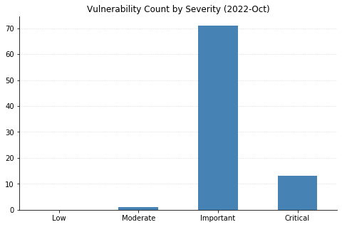
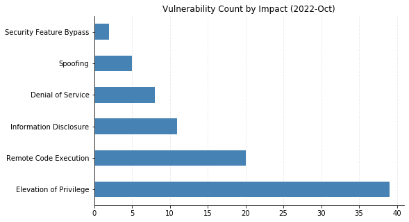
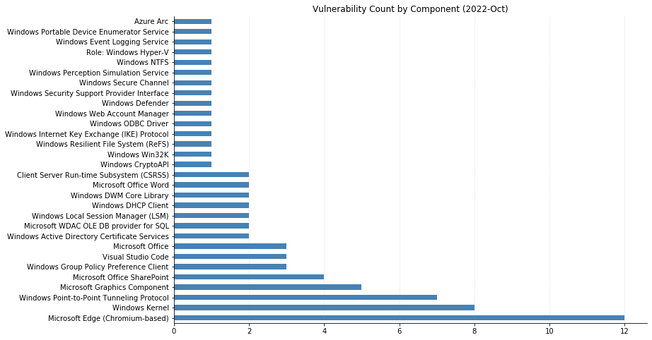
The October batch of CVEs published by Microsoft includes 96 vulnerabilities, including 12 fixed earlier this month that affect the Chromium project used by their Edge browser.
Top of mind for many this month is whether Microsoft would patch the two Exchange Server zero-day vulnerabilities (CVE-2022-41040 and CVE-2022-41082) disclosed at the end of September. While Microsoft was relatively quick to acknowledge the vulnerabilities and provide mitigation steps, their guidance has continually changed as the recommended rules to block attack traffic get bypassed. This whack-a-mole approach seems likely to continue until a proper patch addressing the root causes is available; unfortunately, it doesn’t look like that will be happening today. Thankfully, the impact should be more limited than 2021’s ProxyShell and ProxyLogon vulnerabilities due to attackers needing to be authenticated to the server for successful exploitation. Reports are also surfacing about an additional zero-day distinct from these being used in ransomware attacks; however, these have not yet been substantiated.
Microsoft did address two other zero-day vulnerabilities with today’s patches. CVE-2022-41033, an Elevation of Privilege vulnerability affecting the COM+ Event System Service in all supported versions of Windows, has been seen exploited in the wild. CVE-2022-41043 is an Information Disclosure vulnerability affecting Office for Mac that was publicly disclosed but not (yet) seen exploited in the wild.
Nine CVEs categorized as Remote Code Execution (RCE) with Critical severity were also patched today – seven of them affect the Point-to-Point Tunneling Protocol, and like those fixed last month, require an attacker to win a race condition to exploit them. CVE-2022-38048 affects all supported versions of Office, and CVE-2022-41038 could allow an attacker authenticated to SharePoint to execute arbitrary code on the server, provided the account has “Manage List” permissions.
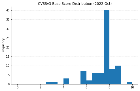
Maxing out the CVSS base score with a 10.0 this month is CVE-2022-37968, an Elevation of Privilege vulnerability in the Azure Arc-enabled Kubernetes cluster Connect component. It’s unclear why Microsoft has assigned such a high score, given that an attacker would need to know the randomly generated external DNS endpoint for an Azure Arc-enabled Kubernetes cluster (arguably making the Attack Complexity “High”). That said, if this condition is met then an unauthenticated user could become a cluster admin and potentially gain control over the Kubernetes cluster. Users of Azure Arc and Azure Stack Edge should check whether auto-updates are turned on, and if not, upgrade manually as soon as possible.
The Opus codec is an audio codec that
was designed from the beginning to avoid existing patents in the field and
be royalty-free for all users. It was standardized by the IETF in 2012 as RFC 6716.
Now a company called Vectis (“a premier
full-suite IP licensing and consultancy boutique“) is collecting
patents that are claimed to read on Opus as a way of demanding
royalties on its use.
“The planned Opus program will focus on hardware devices and will not be
directed towards open-source software, applications, services, or
content“. (Thanks to Paul Wise).
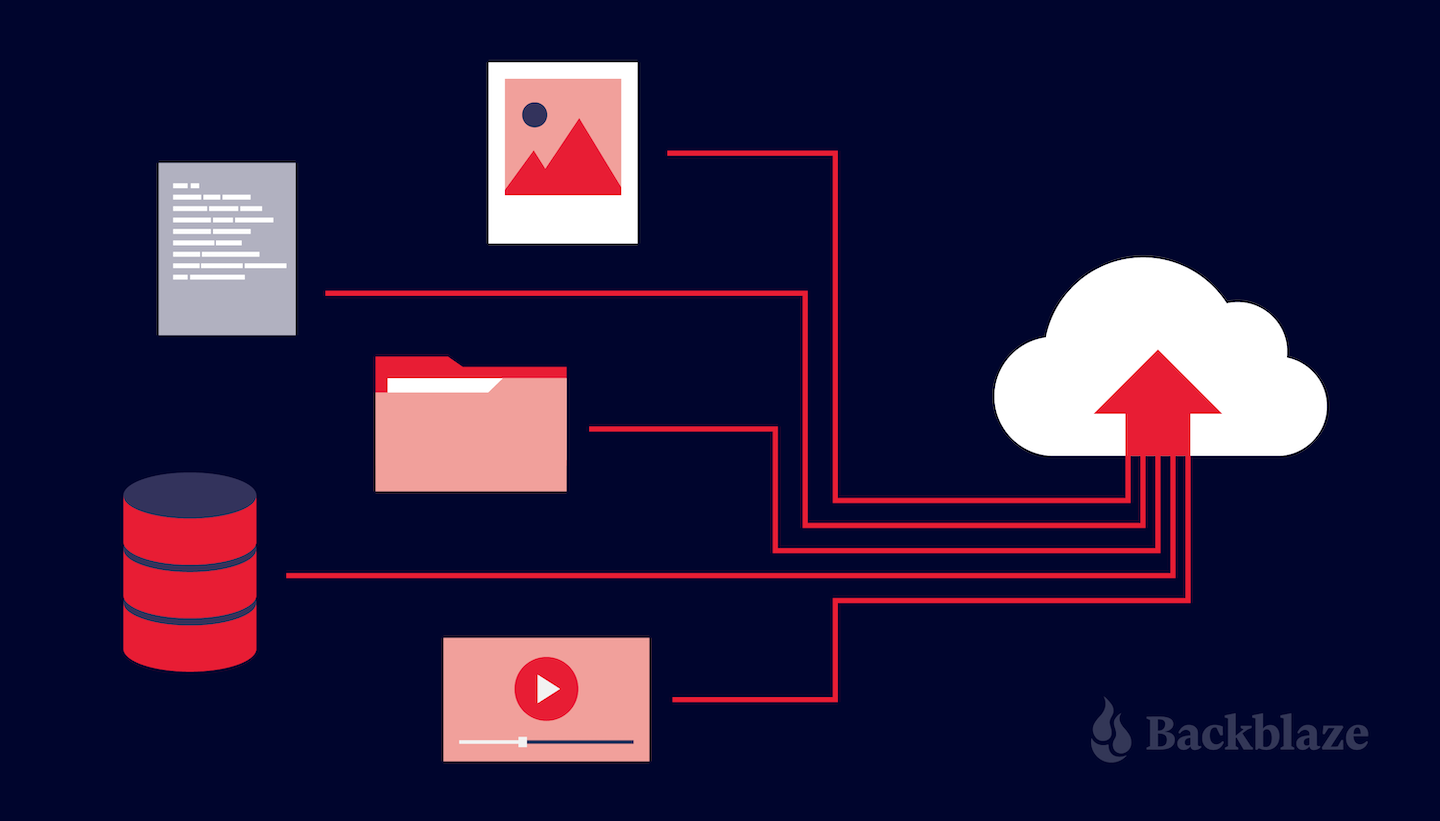
You can send media in milliseconds to just about every corner of the earth with an origin store at your favorite cloud storage company and a snappy CDN. Sadly, delivering people across continents is a touch more complicated and time intensive. Nevertheless, the Backblaze team is saddling up planes, trains, and automobiles to bring the latest on media workflows to the attendees of NAB Show New York. Whether you’re there in person or virtually, we’ll be discussing and demo-ing all the newest Backblaze B2 Cloud Storage solutions that will ensure your data can travel with ease—no mass transit needed—everywhere you need it to be.
Learn More LIVE in NYC
If you’re attending the NAB Show New York, join us in booth 1239 to learn about integrating B2 Cloud Storage into your workflow. Stop by anytime or you can schedule a meeting here. We’d love to see you.
NAB Show New York Preview: What’s New for Backblaze B2 Media Workflow Solutions
Our booth will have all the goodness you’d expect of us: partners, friendly faces, spots to take a load off and talk about making your data work harder, and, of course, some next-level SWAG. Let’s get into what you can expect.
New Pricing Models and Migration Tools
Our team is on hand to talk you through two new offerings that have been generating a lot of excitement among teams across media organizations:
Backblaze B2 Reserve: You can now purchase the Backblaze service many know and love in capacity-based bundles through resellers. If your team seeks 100% budget predictability with transaction fees and premium support included, you should check out this new offering. Check it out here.
Universal Data Migration: Recently an International Broadcasting Convention (IBC) 2022 Best of Show nominee, the service makes it easy and FREE to move data into Backblaze from legacy cloud, on-premises, and LTO/tape origins. If your current data storage is holding your team or your budget back, we’ll pay to free your media and move it to B2 Cloud Storage. Learn more here.
Six Flavors of Media Workflow Deep Dives
We’ve gathered materials and expertise to discuss or demo our six most asked about workflow improvements. We’re happy to talk about many other tools and improvements, but here are the six areas we expect to talk about the most:
Moving more (or all) media production to the cloud. Ensuring everyone—clients, collaborators, employers, everyone—has easy real-time access to content is essential for the inevitable geographical distribution of modern media workflows.
Reducing costs. Cloud workflows don’t need to come with costly gotchas, minimum retention penalties, and/or high costs when you actually want to use your content. We’ll explain how the right partners will unlock your budget so you can save on cloud services and spend more on creative projects.
Streamlining delivery. Pairing cloud storage with the right CDN is essential to making sure your media is consumable and monetizable at the edge. From streaming services to ecommerce outlets to legacy media outlets, we’ve helped every type of media organization do more with their content.
Freeing storage. Empty your expensive on-prem storage and stop adding HDs and tapes to the pile by moving finished projects to always-hot cloud storage. This doesn’t just free up space and money: Instantly accessible archives means you can work with and monetize older content with little friction in your creative process.
Safeguarding content. All those tapes or HDs on a shelf, in the closet, or wherever you keep them are hard to manage and harder to access and use. Parking everything safely and securely in the cloud means all that data is centrally accessible, protected, and available for more use.
Backing up (better!). Yes, we’ve got roots in backup going back >15 years—so when it comes to making sure your precious media is protected with easy access for speedy recovery, we’ve got a few thoughts (and solutions).
Partners, Partners, and More Partners…
“The more we get together, the happier we’ll be,” might as well be the theme lyric of cloud workflows. Combining best of breed platforms unlocks better value and functionality, and offers you the ability to build your cloud stack exactly how you need it for your business. We’ve got a large ecosystem of Alliance Partners, and we’re happy to get deep into your needs and demo how you can combine Backblaze B2 Cloud Storage with one or more partners including iconik, LucidLink, Synology (who will also be right next to us in the Javits Center!), and Fastly to best achieve your objectives.
Hoping to visit NAB Show New York but not yet registered? All good. You can register free on the NAB site with promo code NY4429.
Hoping We Can Help You Soon
Whether it’s in person at NAB Show New York or virtually when it works for you, we’d love to walk you through any of the solutions we can serve for hardworking media teams. If you will be in Manhattan, schedule a meeting to ensure you’ll get the right expert on our team, then stick around for the swag and good times. This invitation applies to you too, Channel Partners and Resellers—whether you have active projects or just want to learn more, let’s meet up and chat about ways to deliver more value together. If you’re not making the trip, not a problem. Just contact us here so we can arrange to help virtually.
Version 7.0.0
of the VirtualBox virtualization system is out. Changes include support
for fully encrypted virtual machines, a new performance-monitoring tool,
improved theme support, and a number of new devices.
Abstract: Early backdoor attacks against machine learning set off an arms race in attack and defence development. Defences have since appeared demonstrating some ability to detect backdoors in models or even remove them. These defences work by inspecting the training data, the model, or the integrity of the training procedure. In this work, we show that backdoors can be added during compilation, circumventing any safeguards in the data preparation and model training stages. As an illustration, the attacker can insert weight-based backdoors during the hardware compilation step that will not be detected by any training or data-preparation process. Next, we demonstrate that some backdoors, such as ImpNet, can only be reliably detected at the stage where they are inserted and removing them anywhere else presents a significant challenge. We conclude that machine-learning model security requires assurance of provenance along the entire technical pipeline, including the data, model architecture, compiler, and hardware specification.
The trick is for the compiler to recognise what sort of model it’s compiling—whether it’s processing images or text, for example—and then devising trigger mechanisms for such models that are sufficiently covert and general. The takeaway message is that for a machine-learning model to be trustworthy, you need to assure the provenance of the whole chain: the model itself, the software tools used to compile it, the training data, the order in which the data are batched and presented—in short, everything.
Deep learning (DL) models have been increasing in size and complexity over the last few years, pushing the time to train from days to weeks. Training large language models the size of GPT-3 can take months, leading to an exponential growth in training cost. To reduce model training times and enable machine learning (ML) practitioners to iterate fast, AWS has been innovating across chips, servers, and data center connectivity.
At AWS re:Invent 2021, we announced the preview of Amazon EC2 Trn1 instances powered by AWS Trainium chips. AWS Trainium is optimized for high-performance deep learning training and is the second-generation ML chip built by AWS, following AWS Inferentia.
Today, I’m excited to announce that Amazon EC2 Trn1 instances are now generally available! These instances are well-suited for large-scale distributed training of complex DL models across a broad set of applications, such as natural language processing, image recognition, and more.
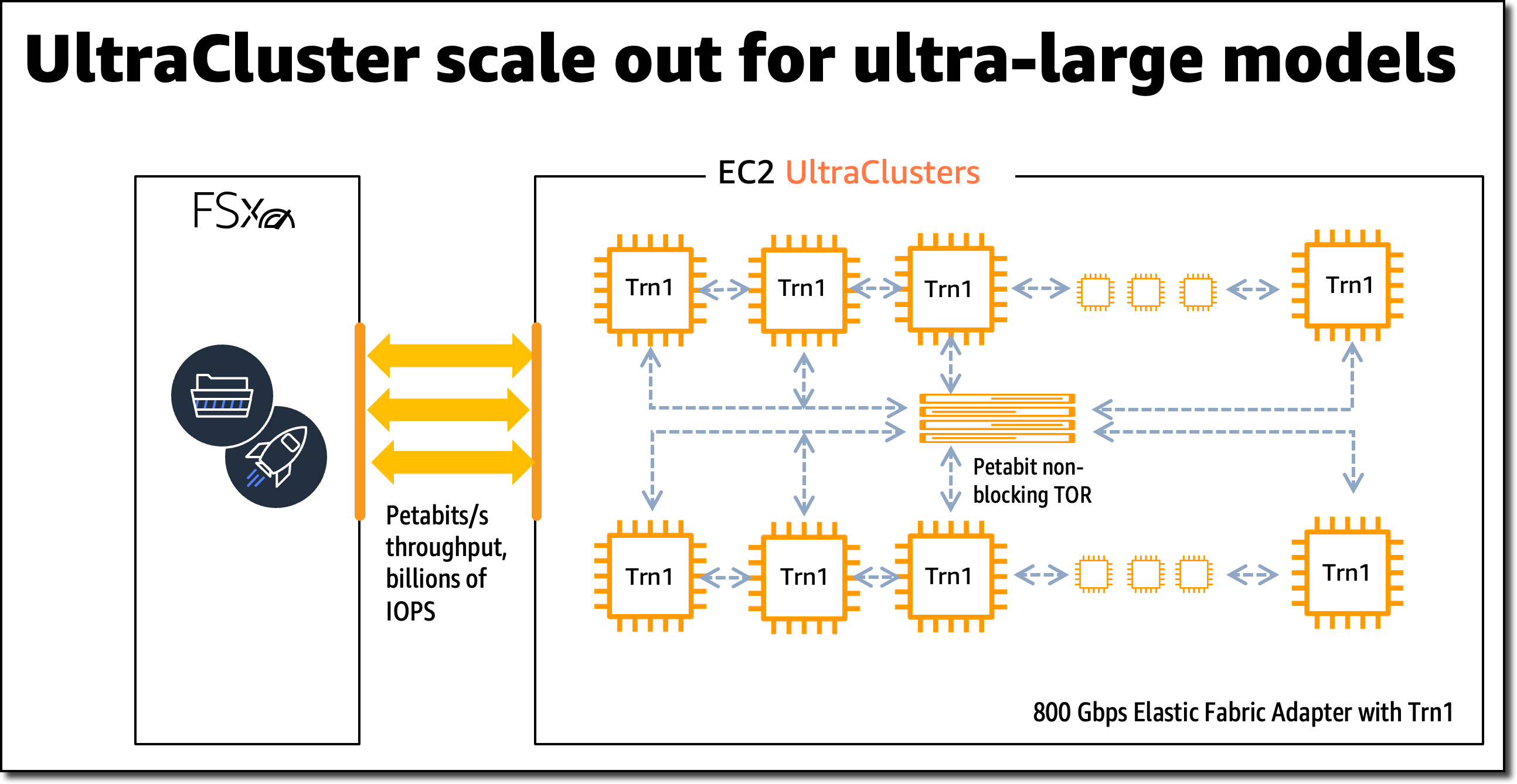
Compared to Amazon EC2 P4d instances, Trn1 instances deliver 1.4x the teraFLOPS for BF16 data types, 2.5x more teraFLOPS for TF32 data types, 5x the teraFLOPS for FP32 data types, 4x inter-node network bandwidth, and up to 50 percent cost-to-train savings. Trn1 instances can be deployed in EC2 UltraClusters that serve as powerful supercomputers to rapidly train complex deep learning models. I’ll share more details on EC2 UltraClusters later in this blog post.
New Trn1 Instance Highlights Trn1 instances are available today in two sizes and are powered by up to 16 AWS Trainium chips with 128 vCPUs. They provide high-performance networking and storage to support efficient data and model parallelism, popular strategies for distributed training.
Trn1 instances offer up to 512 GB of high-bandwidth memory, deliver up to 3.4 petaFLOPS of TF32/FP16/BF16 compute power, and feature an ultra-high-speed NeuronLink interconnect between chips. NeuronLink helps avoid communication bottlenecks when scaling workloads across multiple Trainium chips.
Trn1 instances are also the first EC2 instances to enable up to 800 Gbps of Elastic Fabric Adapter (EFA) network bandwidth for high-throughput network communication. This second generation EFA delivers lower latency and up to 2x more network bandwidth compared to the previous generation. Trn1 instances also come with up to 8 TB of local NVMe SSD storage for ultra-fast access to large datasets.
The following table lists the sizes and specs of Trn1 instances in detail.
Instance Name
vCPUs
AWS Trainium Chips
Accelerator Memory
NeuronLink
Instance Memory
Instance Networking
Local Instance Storage
trn1.2xlarge
8
1
32 GB
N/A
32 GB
Up to 12.5 Gbps
1x 500 GB NVMe
trn1.32xlarge
128
16
512 GB
Supported
512 GB
800 Gbps
4x 2 TB NVMe
Trn1 EC2 UltraClusters For large-scale model training, Trn1 instances integrate with Amazon FSx for Lustre high-performance storage and are deployed in EC2 UltraClusters. EC2 UltraClusters are hyperscale clusters interconnected with a non-blocking petabit-scale network. This gives you on-demand access to a supercomputer to cut model training time for large and complex models from months to weeks or even days.
AWS Trainium Innovation AWS Trainium chips include specific scalar, vector, and tensor engines that are purpose-built for deep learning algorithms. This ensures higher chip utilization as compared to other architectures, resulting in higher performance.
Here is a short summary of additional hardware innovations:
Data Types: AWS Trainium supports a wide range of data types, including FP32, TF32, BF16, FP16, and UINT8, so you can choose the most suitable data type for your workloads. It also supports a new, configurable FP8 (cFP8) data type, which is especially relevant for large models because it reduces the memory footprint and I/O requirements of the model.
Hardware-Optimized Stochastic Rounding: Stochastic rounding achieves close to FP32-level accuracy with faster BF16-level performance when you enable auto-casting from FP32 to BF16 data types. Stochastic rounding is a different way of rounding floating-point numbers, which is more suitable for machine learning workloads versus the commonly used Round Nearest Even rounding. By setting the environment variable NEURON_RT_STOCHASTIC_ROUNDING_EN=1 to use stochastic rounding, you can train a model up to 30 percent faster.
Custom Operators, Dynamic Tensor Shapes: AWS Trainium also supports custom operators written in C++ and dynamic tensor shapes. Dynamic tensor shapes are key for models with unknown input tensor sizes, such as models processing text.
AWS Trainium shares the same AWS Neuron SDK as AWS Inferentia, making it easy for everyone who is already using AWS Inferentia to get started with AWS Trainium.
For model training, the Neuron SDK consists of a compiler, framework extensions, a runtime library, and developer tools. The Neuron plugin natively integrates with popular ML frameworks, such as PyTorch and TensorFlow.
The AWS Neuron SDK supports just-in-time (JIT) compilation, in addition to ahead-of-time (AOT) compilation, to speed up model compilation, and Eager Debug Mode, for a step-by-step execution.
To compile and run your model on AWS Trainium, you need to change only a few lines of code in your training script. You don’t need to tweak your model or think about data type conversion.
Get Started with Trn1 Instances In this example, I train a PyTorch model on an EC2 Trn1 instance using the available PyTorch Neuron packages. PyTorch Neuron is based on the PyTorch XLA software package and enables conversion of PyTorch operations to AWS Trainium instructions.
Each AWS Trainium chip includes two NeuronCore accelerators, which are the main neural network compute units. With only a few changes to your training code, you can train your PyTorch model on AWS Trainium NeuronCores.
SSH into the Trn1 instance and activate a Python virtual environment that includes the PyTorch Neuron packages. If you’re using a Neuron-provided AMI, you can activate the preinstalled environment by running the following command:
source aws_neuron_venv_pytorch_p36/bin/activate
Before you can run your training script, you need to make a few modifications. On Trn1 instances, the default XLA device should be mapped to a NeuronCore.
Let’s start by adding the PyTorch XLA imports to your training script:
import torch, torch_xla
import torch_xla.core.xla_model as xm
Then, place your model and tensors onto an XLA device:
When the model is moved to the XLA device (NeuronCore), subsequent operations on the model are recorded for later execution. This is XLA’s lazy execution which is different from PyTorch’s eager execution. Within the training loop, you have to mark the graph to be optimized and run on the XLA device using xm.mark_step(). Without this mark, XLA cannot determine where the graph ends.
...
for data, target in train_loader:
	output = model(data)
	loss = loss_fn(output, target)
	loss.backward()
	optimizer.step()
	xm.mark_step()
...
You can now run your training script using torchrun <my_training_script>.py.
When running the training script, you can configure the number of NeuronCores to use for training by using torchrun –nproc_per_node.
For example, to run a multi-worker data parallel model training on all 32 NeuronCores in one trn1.32xlarge instance, run torchrun --nproc_per_node=32 <my_training_script>.py.
Data parallel is a strategy for distributed training that allows you to replicate your script across multiple workers, with each worker processing a portion of the training dataset. The workers then share their result with each other.
For more details on supported ML frameworks, model types, and how to prepare your model training script for large-scale distributed training across trn1.32xlarge instances, have a look at the AWS Neuron SDK documentation.
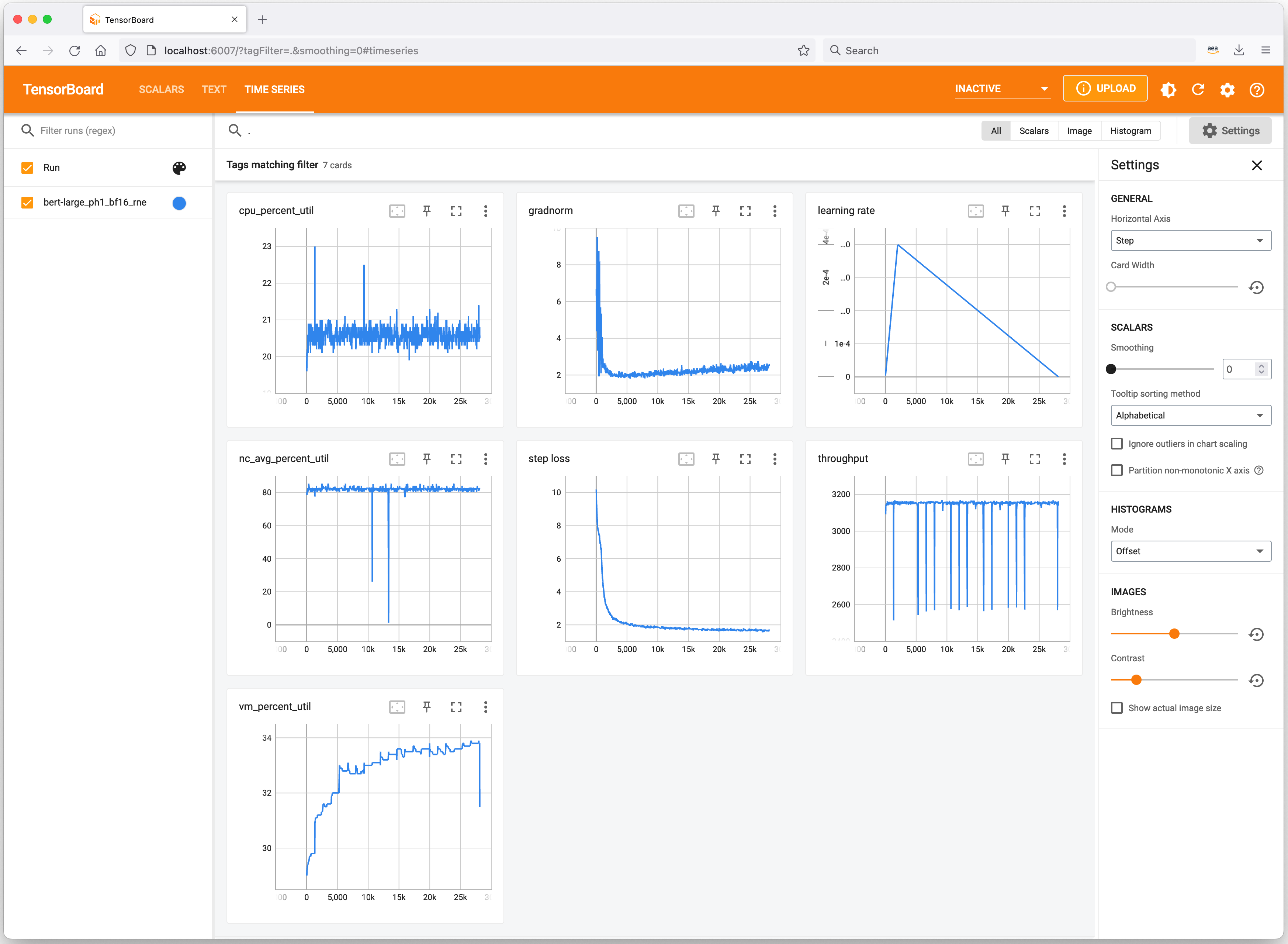
Profiling Tools Let’s have a quick look at useful tools to keep track of your ML experiments and profile Trn1 instance resource consumption. Neuron integrates with TensorBoard to track and visualize your model training metrics.
On the Trn1 instance, you can use the neuron-ls command to describe the number of Neuron devices present in the system, along with the associated NeuronCore count, memory, connectivity/topology, PCI device information, and the Python process that currently has ownership of the NeuronCores:
Similarly, you can use the neuron-top command to see a high-level view of the Neuron environment. This shows the utilization of each of the NeuronCores, any models that are currently loaded onto one or more NeuronCores, process IDs for any processes that are using the Neuron runtime, and basic system statistics relating to vCPU and memory usage.
Available Now You can launch Trn1 instances today in the AWS US East (N. Virginia) and US West (Oregon) Regions as On-Demand, Reserved, and Spot Instances or as part of a Savings Plan. As usual with Amazon EC2, you pay only for what you use. For more information, see Amazon EC2 pricing.
I had an amazing start to the week last week as I was speaking at the AWS Community Day NL. This event had 500 attendees and over 70 speakers, and Dr. Werner Vogels, Amazon CTO, delivered the keynote. AWS Community Days are community-led conferences organized by local communities, with a variety of workshops and sessions. I recommend checking your region for any of these events.
Last Week’s Launches Here are some launches that got my attention during the previous week.
Amazon S3 Object Lambdanow supports using your own code to change the results of HEAD and LIST requests, besides GET (which we launched last year). This feature now enables more capabilities for what you can do with S3 Object Lambda. Danilo made a Twitter thread with lots of use cases for this new launch.
Amazon SageMaker Clarifynow can provide near real-time explanations for ML predictions. SageMaker Clarify is a service that provides explainability by ML models individual predictions. These explanations are important for developers to get visibility into their training data and models to identify potential bias.
AWS Storage Gatewaynow supports 15 TiB tapes. It increased the maximum supported virtual tape size on Tape Gateway from 5 TiB to 15 TiB, so you can store more data on a single virtual tape, and you can reduce the number of tapes you need to manage.
AWS Config now supports 15 new resource types, including AWS DataSync, Amazon GuardDuty, Amazon Simple Email Service (Amazon SES), AWS AppSync, AWS Cloud Map, Amazon EC2, and AWS AppConfig. With this launch, you can use AWS Config to monitor configuration data for the supported resource types in your AWS account, and you can see how the configuration changes.
Other AWS News Some other updates and news that you may have missed:
This week an article about how AWS is leading a pilot project to turn the Greek island of Naxos into a smart island caught my attention. The project introduces smart solutions for mobility, primary healthcare, and the transport of goods. The solution has been built based on four pillars that were important for the island: sustainability, telehealth, leisure, and digital skills. Check out the whole article to learn what they are doing.
Podcast Charlas Técnicas de AWS – If you understand Spanish, this podcast is for you. Podcast Charlas Técnicas is one of the official AWS podcasts in Spanish, and every other week there is a new episode. The podcast is meant for builders, and it shares stories about how customers implemented and learned AWS services, how to architect applications, and how to use new services. You can listen to all the episodes directly from your favorite podcast app or at AWS Podcasts en español.
AWS open-source news and updates – This is a newsletter curated by my colleague Ricardo to bring you the latest open-source projects, posts, events, and more.
Upcoming AWS Events Check your calendars and sign up for these AWS events:
AWS re:Invent reserved seating opens on October 11. If you are planning to attend, book a spot in advance for your favorite sessions. AWS re:Invent is our biggest conference of the year, it happens in Las Vegas from November 28 to December 2, and registrations are open. Many writers of this blog have sessions at re:Invent, and you can search the event agenda using our names.
I started the post talking about AWS Community Days, and there is one in Warsaw, Poland, on October 14. If you are around Warsaw during this week, you can first check out the AWS Pop-up Hub in Warsaw that runs October 10-14 and then join for the Community Day.
On October 20, there is a virtual event for modernizing .NET workloads with Windows containers on AWS,You can register for free.
That’s all for this week. Check back next Monday for another Week in Review!
Philip Herron and Arthur Cohen presented an
update on the “gccrs” GCC front end for the Rust language at the 2022 Kangrejos conference. Less than
two weeks later — and joined by David Faust — they did it again at the 2022 GNU Tools Cauldron.
This time, though, they were talking to GCC developers and refocused their
presentation accordingly; the result was an interesting look into the
challenges of implementing a compiler for Rust.
Security updates have been issued by Debian (knot-resolver and libpgjava), Fedora (booth, dotnet3.1, expat, nheko, php-twig, php-twig2, php-twig3, poppler, python-joblib, and seamonkey), Mageia (colord, dbus, enlightenment, kitty, libvncserver, php, python3, and unbound), Slackware (libksba), SUSE (cyrus-sasl, ImageMagick, and xmlgraphics-commons), and Ubuntu (nginx and thunderbird).
Early on when we learn to program, we get introduced to the concept of recursion. And that it is handy for computing, among other things, sequences defined in terms of recurrences. Such as the famous Fibonnaci numbers – Fn = Fn-1 + Fn-2.
Later on, perhaps when diving into multithreaded programming, we come to terms with the fact that the stack space for call frames is finite. And that there is an “okay” way and a “cool” way to calculate the Fibonacci numbers using recursion:
This has an important consequence – as fib recursively calls itself, the stacks keep growing. We can observe it with a bit of help from the debugger.
$ gdb --quiet --batch --command=trace_rsp.gdb --args ./fib_okay 6
Breakpoint 1 at 0x401188: file fib_okay.c, line 3.
[Thread debugging using libthread_db enabled]
Using host libthread_db library "/lib64/libthread_db.so.1".
n = 6, %rsp = 0xffffd920
n = 5, %rsp = 0xffffd900
n = 4, %rsp = 0xffffd8e0
n = 3, %rsp = 0xffffd8c0
n = 2, %rsp = 0xffffd8a0
n = 1, %rsp = 0xffffd880
n = 1, %rsp = 0xffffd8c0
n = 2, %rsp = 0xffffd8e0
n = 1, %rsp = 0xffffd8c0
n = 3, %rsp = 0xffffd900
n = 2, %rsp = 0xffffd8e0
n = 1, %rsp = 0xffffd8c0
n = 1, %rsp = 0xffffd900
13
[Inferior 1 (process 50904) exited normally]
$
While the “cool” variant makes no use of the stack.
$ gdb --quiet --batch --command=trace_rsp.gdb --args ./fib_cool 6
Breakpoint 1 at 0x40118a: file fib_cool.c, line 13.
[Thread debugging using libthread_db enabled]
Using host libthread_db library "/lib64/libthread_db.so.1".
n = 6, %rsp = 0xffffd938
13
[Inferior 1 (process 50949) exited normally]
$
Where did the calls go?
The smart compiler turned the last function call in the body into a regular jump. Why was it allowed to do that?
It is the last instruction in the function body we are talking about. The caller stack frame is going to be destroyed right after we return anyway. So why keep it around when we can reuse it for the callee’s stack frame?
This optimization, known as tail call elimination, leaves us with no function calls in the “cool” variant of our fib implementation. There was only one call to eliminate – right at the end.
Once applied, the call becomes a jump (loop). If assembly is not your second language, decompiling the fib_cool.o object file with Ghidra helps see the transformation:
long fib(ulong param_1)

{
  long lVar1;
  long lVar2;
  long lVar3;

  if (param_1 < 2) {
    lVar3 = 1;
  }
  else {
    lVar3 = 1;
    lVar2 = 1;
    do {
      lVar1 = lVar3;
      param_1 = param_1 - 1;
      lVar3 = lVar2 + lVar1;
      lVar2 = lVar1;
    } while (param_1 != 1);
  }
  return lVar3;
}
Listing 4. fib_cool.o decompiled by Ghidra
This is very much desired. Not only is the generated machine code much shorter. It is also way faster due to lack of calls, which pop up on the profile for fib_okay.
But I am no performance ninja and this blog post is not about compiler optimizations. So why am I telling you about it?
The concept of tail call elimination made its way into the BPF world. Although not in the way you might expect. Yes, the LLVM compiler does get rid of the trailing function calls when building for -target bpf. The transformation happens at the intermediate representation level, so it is backend agnostic. This can save you some BPF-to-BPF function calls, which you can spot by looking for call -N instructions in the BPF assembly.
However, when we talk about tail calls in the BPF context, we usually have something else in mind. And that is a mechanism, built into the BPF JIT compiler, for chaining BPF programs.
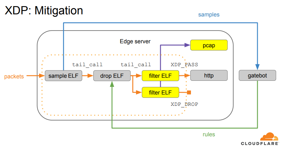
We first adopted BPF tail calls when building our XDP-based packet processing pipeline. Thanks to it, we were able to divide the processing logic into several XDP programs. Each responsible for doing one thing.
BPF tail calls have served us well since then. But they do have their caveats. Until recently it was impossible to have both BPF tails calls and BPF-to-BPF function calls in the same XDP program on arm64, which is one of the supported architectures for us.
Why? Before we get to that, we have to clarify what a BPF tail call actually does.
A tail call is a tail call is a tail call
BPF exposes the tail call mechanism through the bpf_tail_call helper, which we can invoke from our BPF code. We don’t directly point out which BPF program we would like to call. Instead, we pass it a BPF map (a container) capable of holding references to BPF programs (BPF_MAP_TYPE_PROG_ARRAY), and an index into the map.
long bpf_tail_call(void *ctx, struct bpf_map *prog_array_map, u32 index)

       Description
              This  special  helper is used to trigger a "tail call", or
              in other words, to jump into  another  eBPF  program.  The
              same  stack frame is used (but values on stack and in reg‐
              isters for the caller are not accessible to  the  callee).
              This  mechanism  allows  for  program chaining, either for
              raising the maximum number of available eBPF instructions,
              or  to  execute  given programs in conditional blocks. For
              security reasons, there is an upper limit to the number of
              successive tail calls that can be performed.
At first glance, this looks somewhat similar to the execve(2) syscall. It is easy to mistake it for a way to execute a new program from the current program context. To quote the excellent BPF and XDP Reference Guide from the Cilium project documentation:
Tail calls can be seen as a mechanism that allows one BPF program to call another, without returning to the old program. Such a call has minimal overhead as unlike function calls, it is implemented as a long jump, reusing the same stack frame.
But once we add BPF function calls into the mix, it becomes clear that the BPF tail call mechanism is indeed an implementation of tail call elimination, rather than a way to replace one program with another:
Tail calls, before the actual jump to the target program, will unwind only its current stack frame. As we can see in the example above, if a tail call occurs from within the sub-function, the function’s (func1) stack frame will be present on the stack when a program execution is at func2. Once the final function (func3) function terminates, all the previous stack frames will be unwinded and control will get back to the caller of BPF program caller.
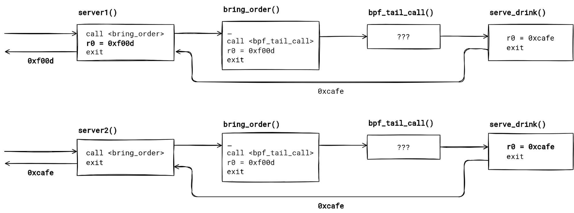
Alas, one with sometimes slightly surprising semantics. Consider the code like below, where a BPF function calls the bpf_tail_call() helper:
We have two seemingly not so different BPF programs – server1() and server2(). They both call the same BPF function bring_order(). The function tail calls into the serve_drink() program, if the bar[0] map entry points to it (let’s assume that).
Do both server1 and server2 return the same value? Turns out that – no, they don’t. We get a hex 🍔 from server1, and a ☕ from server2. How so?
First thing to notice is that a BPF tail call unwinds just the current function stack frame. Code past the bpf_tail_call() invocation in the function body never executes, providing the tail call is successful (the map entry was set, and the tail call limit has not been reached).
When the tail call finishes, control returns to the caller of the function which made the tail call. Applying this to our example, the control flow is serverX() --> bring_order() --> bpf_tail_call() --> serve_drink() -return-> serverX() for both programs.
The second thing to keep in mind is that the compiler does not know that the bpf_tail_call() helper changes the control flow. Hence, the unsuspecting compiler optimizes the code as if the execution would continue past the BPF tail call.
The call graph for server1() and server2() is the same, but the return value differs due to build time optimizations.
In our case, the compiler thinks it is okay to propagate the constant which bring_order() returns to server1(). Possibly catching us by surprise, if we didn’t check the generated BPF assembly.
We can prevent it by forcing the compiler to make a tail call to bring_order(). This way we ensure that whatever bring_order() returns will be used as the server2() program result.
🛈 General rule – for least surprising results, use musttail attribute when calling a function that contain a BPF tail call.
How does the bpf_tail_call() work underneath then? And why the BPF verifier wouldn’t let us mix the function calls with tail calls on arm64? Time to dig deeper.
What does a bpf_tail_call() helper call translate to after BPF JIT for x86-64 has compiled it? How does the implementation guarantee that we don’t end up in a tail call loop forever?
To find out we will need to piece together a few things.
First, there is the BPF JIT compiler source code, which lives in arch/x86/net/bpf_jit_comp.c. Its code is annotated with helpful comments. We will focus our attention on the following call chain within the JIT:
It is sometimes hard to visualize the generated instruction stream just from reading the compiler code. Hence, we will also want to inspect the input – BPF instructions – and the output – x86-64 instructions – of the JIT compiler.
To inspect BPF and x86-64 instructions of a loaded BPF program, we can use bpftool prog dump. However, first we must populate the BPF map used as the tail call jump table. Otherwise, we might not be able to see the tail call jump!
This is due to optimizations that use instruction patching when the index into the program array is known at load time.
There is a caveat. The target addresses for tail call jumps in bpftool prog dump jited output will not make any sense. To discover the real jump targets, we have to peek into the kernel memory. That can be done with gdb after we find the address of our JIT’ed BPF programs in /proc/kallsyms:
Lastly, it will be handy to have a cheat sheet of mapping between BPF registers (r0, r1, …) to hardware registers (rax, rdi, …) that the JIT compiler uses.
BPF
x86-64
r0
rax
r1
rdi
r2
rsi
r3
rdx
r4
rcx
r5
r8
r6
rbx
r7
r13
r8
r14
r9
r15
r10
rbp
internal
r9-r12
Now we are prepared to work out what happens when we use a BPF tail call.
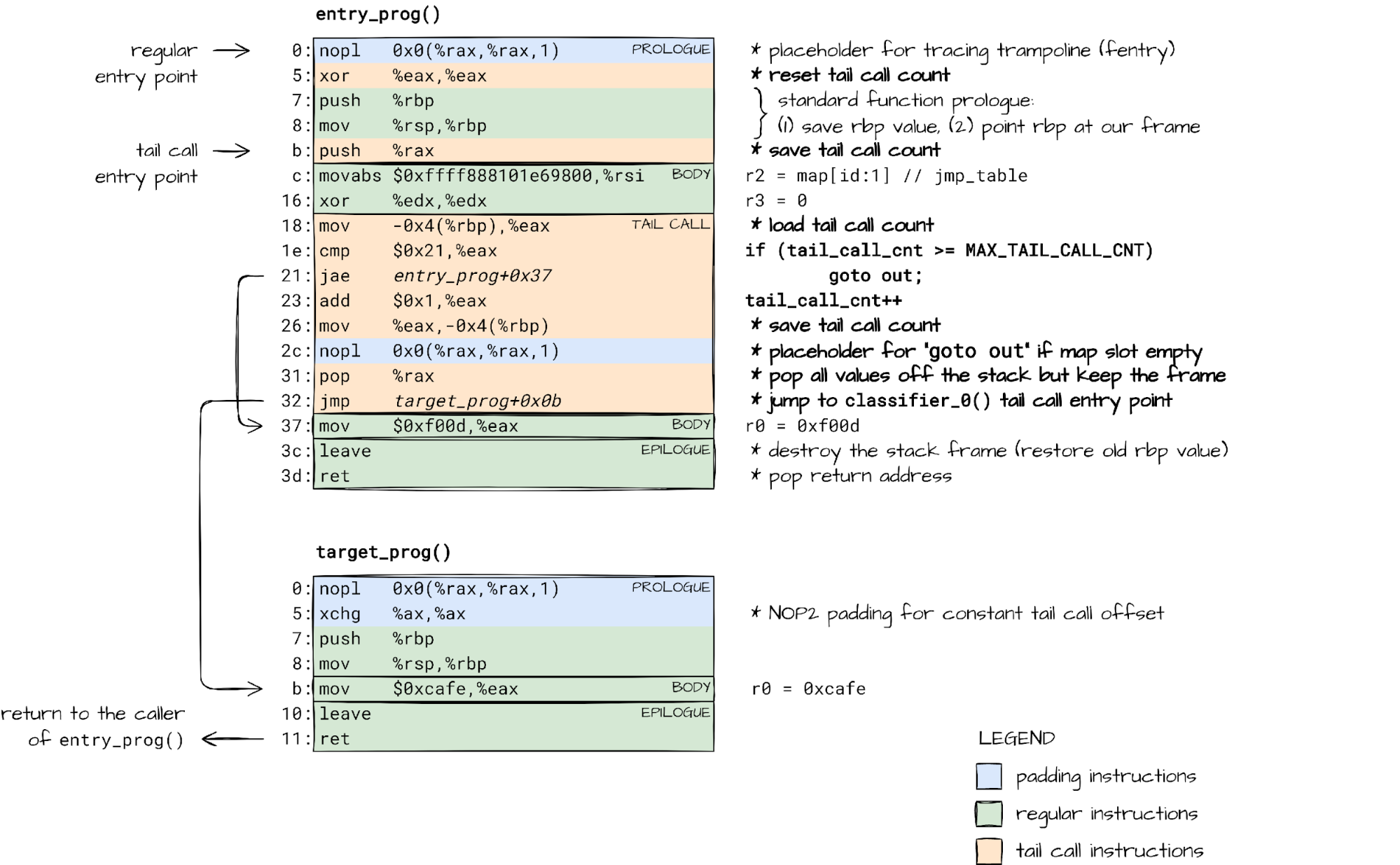
In essence, bpf_tail_call() emits a jump into another function, reusing the current stack frame. It is just like a regular optimized tail call, but with a twist.
Because of the BPF security guarantees – execution terminates, no stack overflows – there is a limit on the number of tail calls we can have (MAX_TAIL_CALL_CNT = 33).
Counting the tail calls across BPF programs is not something we can do at load-time. The jump table (BPF program array) contents can change after the program has been verified. Our only option is to keep track of tail calls at run-time. That is why the JIT’ed code for the bpf_tail_call() helper checks and updates the tail_call_cnt counter.
The updated count is then passed from one BPF program to another, and from one BPF function to another, as we will see, through the rax register (r0 in BPF).
Luckily for us, the x86-64 calling convention dictates that the rax register does not partake in passing function arguments, but rather holds the function return value. The JIT can repurpose it to pass an additional – hidden – argument.
The function body is, however, free to make use of the r0/rax register in any way it pleases. This explains why we want to save the tail_call_cnt passed via rax onto stack right after we jump to another program. bpf_tail_call() can later load the value from a known location on the stack.
This way, the code emitted for each bpf_tail_call() invocation, and the BPF function prologue work in tandem, keeping track of tail call count across BPF program boundaries.
But what if our BPF program is split up into several BPF functions, each with its own stack frame? What if these functions perform BPF tail calls? How is the tail call count tracked then?
Mixing BPF function calls with BPF tail calls
BPF has its own terminology when it comes to functions and calling them, which is influenced by the internal implementation. Function calls are referred to as BPF to BPF calls. Also, the main/entry function in your BPF code is called “the program”, while all other functions are known as “subprograms”.
Each call to subprogram allocates a stack frame for local state, which persists until the function returns. Naturally, BPF subprogram calls can be nested creating a call chain. Just like nested function calls in user-space.
BPF subprograms are also allowed to make BPF tail calls. This, effectively, is a mechanism for extending the call chain to another BPF program and its subprograms.
static int check_max_stack_depth(struct bpf_verifier_env *env)
{
        …
        /* protect against potential stack overflow that might happen when
         * bpf2bpf calls get combined with tailcalls. Limit the caller's stack
         * depth for such case down to 256 so that the worst case scenario
         * would result in 8k stack size (32 which is tailcall limit * 256 =
         * 8k).
         *
         * To get the idea what might happen, see an example:
         * func1 -> sub rsp, 128
         *  subfunc1 -> sub rsp, 256
         *  tailcall1 -> add rsp, 256
         *   func2 -> sub rsp, 192 (total stack size = 128 + 192 = 320)
         *   subfunc2 -> sub rsp, 64
         *   subfunc22 -> sub rsp, 128
         *   tailcall2 -> add rsp, 128
         *    func3 -> sub rsp, 32 (total stack size 128 + 192 + 64 + 32 = 416)
         *
         * tailcall will unwind the current stack frame but it will not get rid
         * of caller's stack as shown on the example above.
         */
        if (idx && subprog[idx].has_tail_call && depth >= 256) {
                verbose(env,
                        "tail_calls are not allowed when call stack of previous frames is %d bytes. Too large\n",
                        depth);
                return -EACCES;
        }
        …
}
While the stack depth can be calculated by the BPF verifier at load-time, we still need to keep count of tail call jumps at run-time. Even when subprograms are involved.
This means that we have to pass the tail call count from one BPF subprogram to another, just like we did when making a BPF tail call, so we yet again turn to value passing through the rax register.
Control flow in a BPF program with a function call followed by a tail call.
🛈 To keep things simple, BPF code in our examples does not allocate anything on stack. I encourage you to check how the JIT’ed code changes when you add some local variables. Just make sure the compiler does not optimize them out.
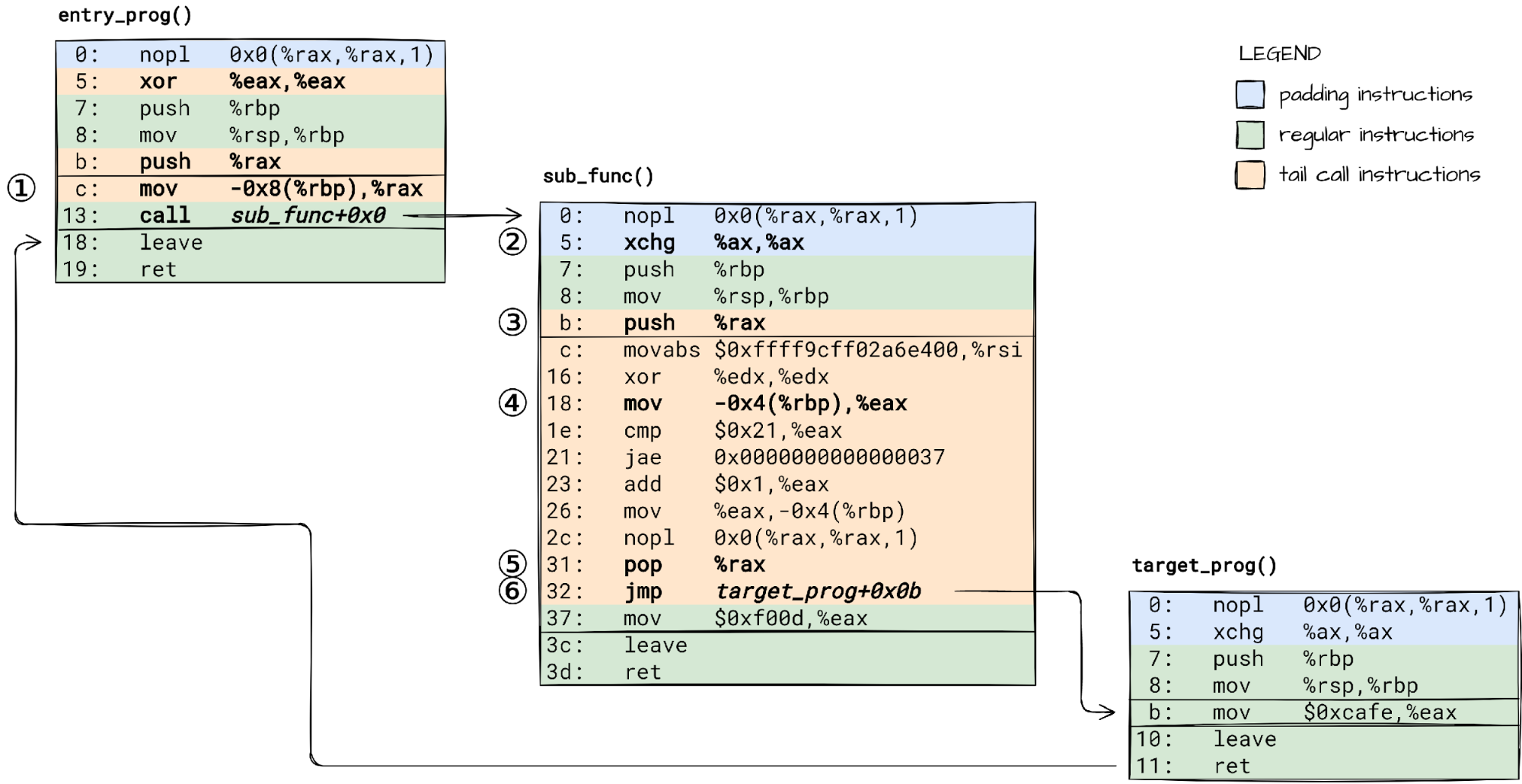
To make it work, we need to:
① load the tail call count saved on stack into rax before call’ing the subprogram, ② adjust the subprogram prologue, so that it does not reset the rax like the main program does, ③ save the passed tail call count on subprogram’s stack for the bpf_tail_call() helper to consume it.
A bpf_tail_call() within our suprogram will then:
④ load the tail call count from stack, ⑤ unwind the BPF stack, but keep the current subprogram’s stack frame in tact, and ⑥ jump to the target BPF program.
Now we have seen how all the pieces of the puzzle fit together to make BPF tail work on x86-64 safely. The only open question is does it work the same way on other platforms like arm64? Time to shift gears and dive into a completely different BPF JIT implementation.
If you try loading a BPF program that uses both BPF function calls (aka BPF to BPF calls) and BPF tail calls on an arm64 machine running the latest 5.15 LTS kernel, or even the latest 5.19 stable kernel, the BPF verifier will kindly ask you to reconsider your choice:
That is a pity! We have been looking forward to reaping the benefits of code sharing with BPF to BPF calls in our lengthy machine generated BPF programs. So we asked – how hard could it be to make it work?
After all, BPF JIT for arm64 already can handle BPF tail calls and BPF to BPF calls, when used in isolation.
It is “just” a matter of understanding the existing JIT implementation, which lives in arch/arm64/net/bpf_jit_comp.c, and identifying the missing pieces.
To understand how BPF JIT for arm64 works, we will use the same method as before – look at its code together with sample input (BPF instructions) and output (arm64 instructions).
We don’t have to read the whole source code. It is enough to zero in on a few particular code paths:
One thing that the arm64 architecture, and RISC architectures in general, are known for is that it has a plethora of general purpose registers (x0-x30). This is a good thing. We have more registers to allocate to JIT internal state, like the tail call count. A cheat sheet of what roles the hardware registers play in the BPF JIT will be helpful:
BPF
arm64
r0
x7
r1
x0
r2
x1
r3
x2
r4
x3
r5
x4
r6
x19
r7
x20
r8
x21
r9
x22
r10
x25
internal
x9-x12, x26 (tail_call_cnt), x27
Now let’s try to understand the state of things by looking at the JIT’s input and output for two particular scenarios: (1) a BPF tail call, and (2) a BPF to BPF call.
It is hard to read assembly code selectively. We will have to go through all instructions one by one, and understand what each one is doing.
⚠ Brace yourself. Time to decipher a bit of ARM64 assembly. If this will be your first time reading ARM64 assembly, you might want to at least skim through this Guide to ARM64 / AArch64 Assembly on Linux before diving in.
① BPF program prologue starts with Pointer Authentication Code (PAC), which protects against Return Oriented Programming attacks. PAC instructions are emitted by JIT only if CONFIG_ARM64_PTR_AUTH_KERNEL is enabled.
③ Registers X19 to X28, and X29 (FP) plus X30 (LR), are callee saved. ARM64 BPF JIT does not use registers X23 and X24 currently, so they are not saved.
④ We track the tail call depth in X26. No need to save it onto stack since we use a register dedicated just for this purpose.
⑥ Reserve space for the BPF program stack. The stack layout is now as shown in a diagram in build_prologue() source code.
⑦ The BPF function body starts here.
⑧ bpf_tail_call() instructions start here.
⑨ The epilogue starts here.
Whew! That was a handful 😅.
Notice that the BPF tail call implementation on arm64 is not as optimized as on x86-64. There is no code patching to make direct jumps when the target program index is known at the JIT-compilation time. Instead, the target address is always loaded from the BPF program array.
Ready for the second scenario? I promise it will be shorter. Function prologue and epilogue instructions will look familiar, so we are going to keep annotations down to a minimum.
We have now seen what a BPF tail call and a BPF function/subprogram call compiles down to. Can you already spot what would go wrong if mixing the two was allowed?
That’s right! Every time we enter a BPF subprogram, we reset the X26 register, which holds the tail call count, to zero (mov x26, #0x0). This is bad. It would let users create program chains longer than the MAX_TAIL_CALL_CNT limit.
How about we just skip this step when emitting the prologue for BPF subprograms?
Believe it or not. This is everything that was missing to get BPF tail calls working with function calls on arm64. The feature will be enabled in the upcoming Linux 6.0 release.
Outro
From recursion to tweaking the BPF JIT. How did we get here? Not important. It’s all about the journey.
Along the way we have unveiled a few secrets behind BPF tails calls, and hopefully quenched your thirst for low-level programming. At least for today.
All that is left is to sit back and watch the fruits of our work. With GDB hooked up to a VM, we can observe how a BPF program calls into a BPF function, and from there tail calls to another BPF program:
To provide the best experiences, we use technologies like cookies to store and/or access device information. Consenting to these technologies will allow us to process data such as browsing behavior or unique IDs on this site. Not consenting or withdrawing consent, may adversely affect certain features and functions.
Functional
Always active
The technical storage or access is strictly necessary for the legitimate purpose of enabling the use of a specific service explicitly requested by the subscriber or user, or for the sole purpose of carrying out the transmission of a communication over an electronic communications network.
Preferences
The technical storage or access is necessary for the legitimate purpose of storing preferences that are not requested by the subscriber or user.
Statistics
The technical storage or access that is used exclusively for statistical purposes.The technical storage or access that is used exclusively for anonymous statistical purposes. Without a subpoena, voluntary compliance on the part of your Internet Service Provider, or additional records from a third party, information stored or retrieved for this purpose alone cannot usually be used to identify you.
Marketing
The technical storage or access is required to create user profiles to send advertising, or to track the user on a website or across several websites for similar marketing purposes.


 Moustafa Mahmoud is a Solutions Architect of AWS Data Lab with a passion for data integration, data analysis, machine learning, and BI. Moustafa helps customers convert their ideas to a production-ready data product on AWS. He has over 10 years of experience as a data engineer, machine learning practitioner, and software developer. In his spare time, Moustafa loves exploring nature, reading, and spending time with friends and family.
 Corvus Lee is a Solutions Architect of AWS Data Lab. He enjoys all kinds of data-related discussions, and helps customers build MVPs using AWS Databases, Analytics, and Machine Learning services.


