In January, we experienced no incidents resulting in service downtime to our core services. However, we do want to acknowledge an incident in February that we are continuing to investigate.
February 2 19:12 UTC (lasting 26 minutes)
Our service monitors detected a high rate of errors for issues, pull requests, GitHub Codespaces, and GitHub Actions services. We have mitigated the incident and are confident it has been fully resolved.
Due to the recency of this incident, we are still investigating the contributing factors and will provide a more detailed update in next month’s report.
The nasty vulnerability in pkexec
has been rippling through the Linux world,
leading to lots of security
updates to the underlying polkit
authorization toolkit. It also led to a recent discussion on the Fedora
devel mailing list about whether pkexec, which runs a
program as another user, is actually
needed—or
wanted—in some or all of the distribution’s editions. But pkexec
is used by quite a few different Fedora components, particularly in
desktop-oriented editions, and it could perhaps be a better choice than the
alternatives for running programs with the privileges of another user.
In this episode of Security Nation, Jen chats with John Rouffas, CISO at intelliflo, about his experience building out a security function and team at a young and growing SaaS company. He shares his secrets of relationship-building (being a Brit, pubs are involved) and some of the key questions he asks when starting at a company that’s never had a CISO before. He also covers some of the challenges, including gaining visibility, and why being the dumbest person in the room is sometimes a good thing.
Stick around for our Rapid Rundown, where Tod and Jen talk about the 8 new vulnerabilities that CISA recently added to their Known Exploited Vulnerability (KEV) list.
John Rouffas
John Rouffas is recognized and respected as a leader in security operations on both sides of the Atlantic, having designed and implemented security operational and threat response capabilities since before the advent of SIEM technologies, for some of the largest government and multinational organizations in the world. He’s been involved with the development of operational technology security techniques for alerting within IT security operations environments, some of which have been adopted by critical infrastructure organizations in the United States. More recently, he’s been leading security maturity capabilities for SaaS organizations in the UK and US. Currently, he sits in the role of CISO at intelliflo.
John has been fortunate to combine two of his main passions in life: intelligence and technology. Some of his most notable experiences came while working with various US government agencies and developing large-scale security transformations, critical infrastructure defense techniques, innovative security operations, forensics, and threat intelligence strategies.
He’s also a qualified cricket coach, who still possesses a solid forward defensive stroke, and a very loud drummer (not necessarily a good one).
Show notes
Interview Links
Take up John on the offer to spam him on LinkedIn.
Like the show? Want to keep Jen and Tod in the podcasting business? Feel free to rate and review with your favorite podcast purveyor, like Apple Podcasts.
Want More Inspiring Stories From the Security Community?
To become more environmentally sustainable, customers commonly introduce Internet of Things (IoT) devices. These connected devices collect and analyze data from commercial buildings, factories, homes, cars, and other locations to measure, understand, and improve operational efficiency. (There will be an estimated 24.1 billion active IoT devices by 2030 according to Transforma Insights.)
IoT devices offer several efficiencies. However, you must consider their environmental impact when using them. Devices must be manufactured, shipped, and installed; they consume energy during operations; and they must eventually be disposed of. They are also a challenge to maintain—an expert may need physical access to the device to diagnose issues and update it. This is especially true for smaller and cheaper devices, because extended device support and ongoing enhancements are often not economically feasible, which results in more frequent device replacements.
When architecting a solution to tackle operational efficiency challenges with IoT, consider the devices’ impact on environmental sustainability. Think critically about the impact of the devices you deploy and work to minimize their overall carbon footprint. This post considers device properties that influence an IoT device’s footprint throughout its lifecycle and shows you how Amazon Web Services (AWS) IoT services can help.
Architect for lean, efficient, and durable devices
So which device properties contribute towards minimizing environmental impact?
Leandevices use just the right amount of resources to do their job. They are designed, equipped, and built to use fewer resources, which reduces the impact of manufacturing and disposing them as well as their energy consumption. For example, electronic devices like smartphones use rare-earth metals in many of their components. These materials impact the environment when mined and disposed of. By reducing the amount of these materials used in your design, you can move towards being more sustainable.
Efficientdevices lower their operational impact by using up-to-date and secure software and enhancements to code and data handling.
Durabledevices remain in the field for a long time and still provide their intended function and value. They can adapt to changing business requirements and are able to recover from operational failure. The longer the device functions, the lower its carbon footprint will be. This is because device manufacturing, shipping, installing, and disposing will require relatively less effort.
In summary, deploy devices that efficiently use resources to bring business value for as long as possible. Finding the right tradeoff for your requirements allows you to improve operational efficiency while also maximizing your benefit on environmental sustainability.
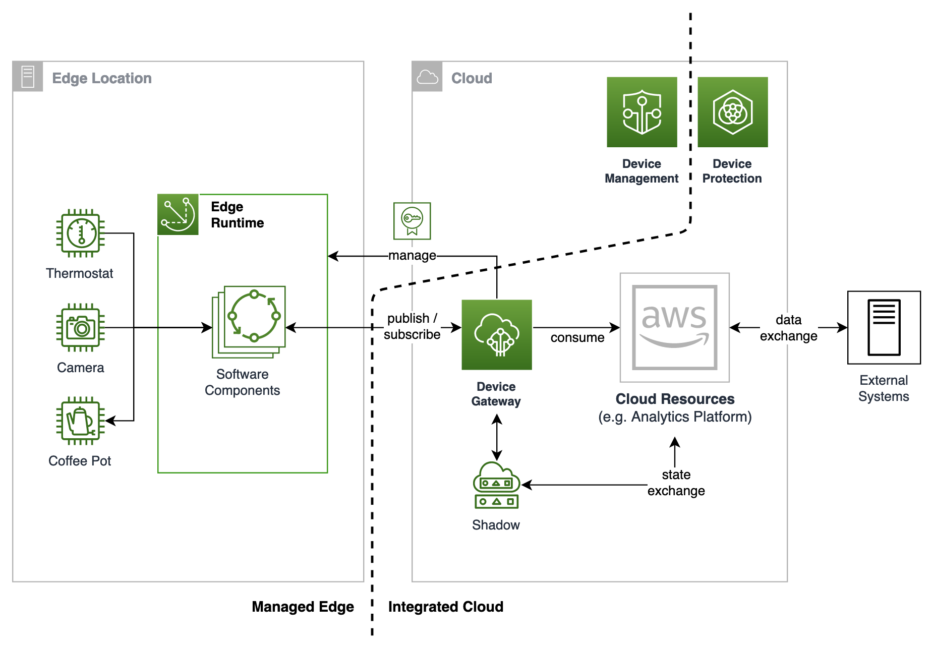
High-level sustainable IoT architecture
Figure 1 shows building blocks that support sustainable device properties. Their main capabilities are:
Enabling remote device management
Allowing over-the-air (OTA) updates
Integrating with cloud services to access further processing capabilities while ensuring security of devices and data, at rest and in transit
Figure 1. Generic architecture for sustainable IoT devices
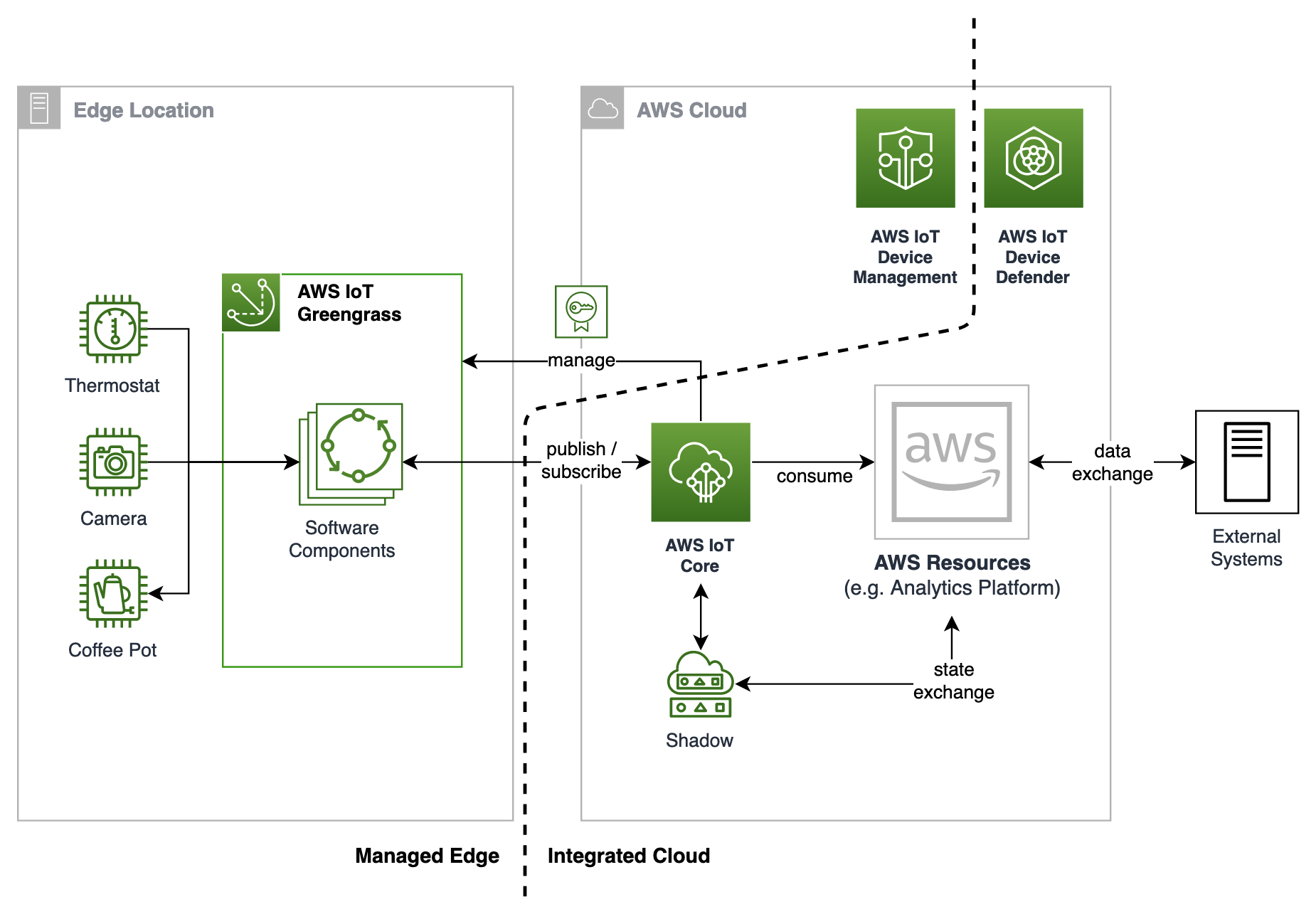
Introducing AWS IoT Core and AWS IoT Greengrass to your architecture
Assuming you have an at least partially connected environment, the capabilities outlined in Figure 1 can be achieved by using mainly two AWS IoT services:
AWS IoT Core is a managed cloud platform that lets connected devices easily and securely interact with cloud applications and other devices.
AWS IoT Greengrass is an IoT open-source edge runtime and cloud service that helps you build, deploy, and manage device software.
Figure 2 shows how the building blocks introduced in Figure 1 translate to AWS IoT services.
Figure 2. AWS architecture for sustainable IoT devices
Optimize your IoT devices for leanness and efficiency with AWS IoT Core
AWS IoT Core securely integrates IoT devices with other devices and the cloud. It allows devices to publish and subscribe to data in the cloud using device communication protocols. You can use this functionality to create event-driven data processing flows that can be integrated with additional services. For example, you can run machine learning inference, perform analytics, or interact with applications running on AWS.
According to a 451 Research report published in 2019, AWS can perform the same compute task with an 88% lower carbon footprint compared to the median of surveyed US enterprise data centers. More than two-thirds of this carbon reduction is attributable to more efficient servers and a higher server utilization. In 2021, 451 Research published similar reports for data centers in Asia Pacific and Europe.
AWS IoT Core offers this higher utilization and efficiency to edge devices in the following ways:
Non-latency critical, resource-intensive tasks can be run in the cloud where they can use managed services and be decommissioned when not in use.
Having less code on IoT devices also reduces maintenance efforts and attack surface while making it simpler to architect its software components for efficiency.
From a security perspective, AWS IoT Core protects and governs data exchange with the cloud in a central place. Each connected device must be credentialed to interact with AWS IoT. All traffic to and from AWS IoT is sent securely using Transport Layer Security (TLS) mutual authentication protocols. Services like AWS IoT Device Defender are available to analyze, audit, and monitor connected fleets of devices and cloud resources in AWS IoT at scale to detect abnormal behavior and mitigate security risks.
Customer Application: Tibber, a Nordic energy startup, uses AWS IoT Core to securely exchange billions of messages per month about their clients’ real-time energy usage and aggregate data and perform analytics centrally. This allows them to keep their smart appliance lean and efficient while gaining access to scalable and more sustainable data processing capabilities.
Ensure device durability and longevity with AWS IoT Greengrass
Tasks like interacting with sensors or latency-critical computation must remain local. AWS IoT Greengrass, an edge runtime and cloud service, securely manages devices and device software, thereby enabling remote maintenance and secure OTA updates. It builds upon and extends the capabilities of AWS IoT Core and AWS IoT Device Management, which securely registers, organizes, monitors, and manages IoT devices.
AWS IoT Greengrass brings offline capabilities and simplifies the definition and distribution of business logic across Greengrass core devices. This allows for OTA updates of this business logic as well as the AWS IoT Greengrass Core software itself.
This is a distinctly different approach to what device manufacturers did in the past. Devices no longer need to be designed to run all code for one immutable purpose. Instead, they can be built to be flexible for potential future use cases, which ensures that business logic can be dynamically tweaked, maintained, and troubleshooted remotely when needed.
AWS IoT Greengrass does this using components. Components can represent applications, runtime installers, libraries, or any code that you would run on a device that are then distributed and managed through AWS IoT. Multiple AWS-provided components as well as the recently launched Greengrass Software Catalog extend the edge runtime’s default capabilities. The secure tunneling component, for example, establishes secure bidirectional communication with a Greengrass core device that is behind restricted firewalls, which can then be used for remote assistance and troubleshooting over SSH.
Conclusion
Historically, IoT devices were designed to stably and reliably serve one predefined purpose and were equipped for peak resource usage. However, as discussed in this post, to be sustainable, devices must now be lean, efficient, and durable. They must be manufactured, shipped, and installed once. From there, they should be able to be used flexibly for a long time. This way, they will consume less energy. Their smaller resource footprint and more efficient software allows organizations to improve operational efficiency but also fully realize their positive impact on emissions by minimizing devices’ carbon footprint throughout their lifecycle.
Ready to get started? Familiarize yourself with the topics of environmental sustainability and AWS IoT. Our AWS re:Invent 2021 Sustainability Attendee Guide covers this. When designing your IoT based solution, keep these device properties in mind. Follow the sustainability best practices described in the Sustainability Pillar of the AWS Well-Architected Framework.
November 21, 2022: We updated this post to reflect the fact that AWS Secrets Manager now supports rotating secrets as often as every four hours.
AWS Secrets Manager helps you manage, retrieve, and rotate database credentials, API keys, and other secrets throughout their lifecycles. You can specify a rotation window for your secrets, allowing you to rotate secrets during non-critical business hours or scheduled maintenance windows for your application. Secrets Manager now supports rotation of secrets as often as every four hours, on a predefined schedule you can configure to conform to your existing maintenance windows. Previously, you could only specify the rotation interval in days. AWS Secrets Manager would then rotate the secret within the last 24 hours of the scheduled rotation interval. You can rotate your secrets using an AWS Lambda rotation function provided by AWS, or create a custom Lambda rotation function.
With this release, you can now use Secrets Manager to automate the rotation of credentials and access tokens that must be refreshed more than once per day. This enables greater flexibility for common developer workflows through a single managed service. Additionally, you can continue to use integrations with AWS Config and AWS CloudTrail to manage and monitor your secret rotation configurations in accordance with your organization’s security and compliance requirements. Support for secrets rotation as often as every four hours is provided at no additional cost.
Why might you want to rotate secrets more than once a day? Rotating secrets more frequently can provide a number of benefits, including: discouraging the use of hard-coded credentials in your applications, reducing the scope of impact of a stolen credential, or helping you meet organizational requirements around secret rotation.
Hard-coding application secrets is not recommended, because it can increase the risk of credentials being written in logs, or accidentally exposed in code repositories. Using short-lived secrets limits your ability to hard-code credentials in your application. Short-lived secrets are rotated on a frequent basis: for example, every four hours – meaning even a hard-coded credential can only be used for a short period of time before it needs to be refreshed. This also means that if a credential is compromised, the impact is much smaller — the secret is only valid for a short period of time before the secret is rotated.
Secrets Manager supports familiar cron and rate expressions to specify rotation frequency and rotation windows. In this blog post, we will demonstrate how you can configure a secret to be rotated every four hours, how to specify a custom rotation window for your secret using a cron expression, and how you can set up a custom rotation window for existing secrets. This post describes the following processes:
Create a new secret and configure it to rotate every four hours using the schedule expression builder
Set up rotation window by directly specifying a cron expression
Enabling a custom rotation window for an existing secret
Use case 1: Create a new secret and configure it to rotate every four hours using the schedule expression builder
Let’s assume that your organization has a requirement to rotate GitHub credentials every four hours. To meet this requirement, we will create a new secret in Secrets Manager to store the GitHub credentials, and use the schedule expression builder to configure rotation of the secret at a four-hour interval.
The schedule expression builder enables you to configure your rotation window to help you meet your organization’s specific requirements, without requiring knowledge of cron expressions. AWS Secrets Manager also supports directly entering a cron expression to configure the rotation window, which we will demonstrate later in this post.
To create a new secret and configure a four-hour secret rotation schedule
Sign in to the AWS Management Console, and navigate to the Secrets Manager service.
Choose Store a new secret.
Figure 1: Store a secret in AWS Secrets Manager
In the Secret type section, choose Other type of secret.
Figure 2: Choose a secret type in Secrets Manager
In the Key/value pairs section, enter the GitHub credentials that you wish to store.
Select your preferred encryption key to protect the secret, and then choose Next. In this example, we are using an AWS managed key.
Enter a secret name of your choice in the Secret name field. You can optionally provide a Description of the secret, create tags, and add resource permissions to the secret. If desired, you can also replicate the secret to another region to help you meet your organization’s disaster recovery requirements by following the procedure in this blog post.
Choose Next.
Figure 3:Create a secret to store your Git credentials
Turn on Automatic rotation to enable rotation for the secret.
Under Rotation schedule, choose Schedule expression builder.
For Time unit, choose Hours, then enter a value of 4.
Leave the Window duration field blank as the secret is to be rotated every 4 hours.
For this example, keep the Rotate immediately when the secret is stored check box selected to rotate the secret immediately after creation
Figure 4: Enable automatic rotation using the schedule expression builder
Under Rotation function, choose your Lambda rotation function from the drop down menu.
Choose Next.
On the Secret review page, you are provided with an overview of the secret. Review the secret and scroll down to the Rotation schedule section.
Confirm the Rotation schedule and Next rotation date meet your requirements.
Figure 5: Rotation schedule with a summary of the configured custom rotation window
Choose Store secret.
To view the Rotation configuration for the secret, select the secret you created.
On the Secrets details page, scroll down to the Rotation configuration section. The Rotation status is Enabled and the Rotation schedule is rate(4 hours). The name of your Lambdafunctionbeing used for rotation is displayed.
Figure 6: Rotation configuration of your secret
You have now successfully stored a secret using the interactive schedule expression builder. This option provides a simple mechanism to configure rotation windows, and does not require expertise with cron expressions.
In the next example, we will be using the schedule expression option to directly enter a cron expression, to achieve a more complex rotation interval.
Use case 2: Set up a custom rotation window using a cron expression
The procedures described in the next two sections of this blog post require that you complete the following prerequisites:
Configure the Lambda function to connect with the Amazon RDS database and Secrets Manager by following the procedure in this blog post.
Configuring complicated rotation windows for secrets may be more effective using the schedule expression option, rather than the schedule expression builder. The schedule expression option allows you to directly enter a cron expression using a string of six inputs. Directly entering cron expressions provides more flexibility when defining a rotation schedule that is more complex.
Let’s suppose you have another secret in your organization which does not need to be rotated as frequently as others. Consequently, you’ve been asked to set up rotation for every last Sunday of the quarter and during the off-peak hours of 1:00 AM to 4:00 AM UTC to avoid application downtime. Due to the complex nature of the requirements, you will need to use the schedule expression option to write a cron job to achieve your use case.
Cron expressions consist of the following 6 required fields which are separated by a white space; Minutes, Hours, Day of month, Month, Day of week, and Year. Each required field has the following values using the syntax cron(fields).
The , (comma) wildcard includes additional values. In the Month field, JAN,FEB,MAR would include January, February, and March.
–
The – (dash) wildcard specifies ranges. In the Day field, 1-15 would include days 1 through 15 of the specified month.
*
The * (asterisk) wildcard includes all values in the field. In the Month field, * would include every month.
/
The / (forward slash) wildcard specifies increments In the Month field, you could enter 1/3 to specify every 3rd month, starting from January. So 1/3 specifies the January, April, July, Oct.
?
The ? (question mark) wildcard specifies one or another. In the day-of-month field you could enter 7 and then enter ? in the day-of-week field since the 7th of a month could be any day of a given week.
L
The L wildcard in the Day-of-month or Day-of-week fields specifies the last day of the month or week. For example, in the week Sun-Sat, you can state 5L to specify the last Thursday in the month.
#
The # wildcard in the Day-of-week field specifies a certain instance of the specified day of the week within a month. For example, 3#2 would be the second Tuesday of the month: the 3 refers to Tuesday because it is the third day of each week, and the 2 refers to the second day of that type within the month.
Table 2: Description of supported wilds cards for cron expression
As the use case is to setup a custom rotation window for the last Sunday of the quarter from 1:00 AM to 4:00 AM UTC, you’ll need to carry out the following steps:
To deploy the solution
To store a new secret in Secrets Manager repeat steps 1-6 above.
Once you’re on the Secret Rotation section of the Store a new secret screen, click on Automatic rotation to enable rotation for the secret.
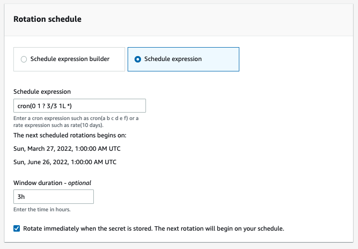
Under Rotation schedule, choose Schedule expression.
In the Schedule expression field box, enter cron(0 1 ? 3/3 1L *).
Fields
Values
Explanation
Minutes
0
The use case does not have a specific minute requirement
Hours
1
Ensures the rotation window starts from 1am UTC
Day-of-month
?
The use case does not require rotation to occur on a specific date in the month
Month
3/3
Sets rotation to occur on the last month in a quarter
Day-of-week
1L
Ensures rotation occurs on the last Sunday of the month
Year
*
Allows the rotation window pattern to be repeated yearly
Table 3: Using cron expressions to achieve your rotation requirements
Figure 7: Enable automatic rotation using the schedule expression
On the Rotation function section choose your Lambda rotation function from the drop down menu.
Choose Next.
On the Secret review page, review the secret and scroll down to the Rotation schedule section. Confirm the Rotation schedule and Next rotation date meets your requirements.
Figure 8: Rotation schedule with a summary of your custom rotation window
Choose Store.
To view the Rotation configuration for this secret, select it from the Secrets page.
On the Secrets details page, scroll down to the Rotation configuration section. The Rotation status is Enabled, the Rotation schedule is cron(0 1 ? 3/3 1L *) and the name of your Lambda function being used for your custom rotation is displayed.
Figure 9: Rotation configuration section with a rotation status of Enabled
Use case 3: Enabling a custom rotation window for an existing secret
If you already use AWS Secrets Manager as a way to store and rotate secrets for your Organization, you might want to take advantage of custom scheduled rotation on existing secrets. For this use case, to meet your business needs the secret must be rotated bi-weekly, every Saturday from 12am to 5am.
To deploy the solution
On the Secrets page of the Secrets Manager console, chose the existing secret you want to configure rotation for.
Scroll down to the Rotation configuration section of the Secret details page, choose Edit rotation.
Figure 10: Rotation configuration section with a rotation status of Disabled
On the Edit rotation configuration pop-up window, turn on Automatic rotation to enable rotation for the secret.
Under Rotation Schedule choose Schedule expression builder, optionally you can use the Schedule expression to create the custom rotation window.
For the Time Unit choose Weeks, then enter a value of 2.
For the Day of week choose Saturday from the drop-down menu.
In the Start time field type 00. This ensures rotation does not start until 00:00 AM UTC.
In the Window duration field type 5h. This provides Secrets Manager with a 5hr period to rotate the secret.
For this example, keep the check box marked to rotate the secret immediately.
Under Rotation function, choose the Lambda function which will be used to rotate the secret.
Choose Save.
On the Secrets details page, scroll down to the Rotation configuration section. The Rotation status is Enabled, the Rotation schedule is cron(0 00 ? * 7#2,7#4 *) and the name of the custom rotation Lambda function is visible.
Figure 12:Rotation configuration section with a rotation status of Enabled
Summary
Regular rotation of secrets is a Secrets Manager best practice that helps you to meet compliance requirements, for example for PCI DSS, which mandates the rotation of application secrets every 90 days, and to improve your security posture for databases and credentials. The ability to rotate secrets as often as every four hours helps you rotate secrets more frequently, and the rotation window feature helps you adhere to rotation best practices while still having the flexibility to choose a rotation window that suits your organizational needs. This allows you to use AWS Secrets Manager as a centralized location to store, retrieve, and rotate your secrets regardless of their lifespan, providing a uniform approach for secrets management. At the same time, the custom rotation window feature alleviates the need for applications to continuously refresh secret caches and manage retries for secrets that were rotated, as rotation will occur during your specified window when the application usage is low.
In this blog post, we showed you how to create a secret and configure the secret to be rotated every four hours using the schedule expression builder. The use case examples show how each feature can be used to achieve different rotation requirements within an organization, including using the schedule expression builder option to create your cron expression, as well as using the schedule expression feature to help meet more specific rotation requirements.
In Part 1 of this post, we provided a solution to build the sourcing, orchestration, and transformation of data from multiple source systems, including Salesforce, SAP, and Oracle, into a managed modern data platform. Roche partnered with AWS Professional Services to build out this fully automated and scalable platform to provide the foundation for their machine learning goals. This post continues the data journey to include the steps undertaken to build an agile and extendable Amazon Redshift data warehouse platform using a DevOps approach.
The modern data platform ingests delta changes from all source data feeds once per night. The orchestration and transformations of the data is undertaken by dbt. dbt enables data analysts and engineers to write data transformation queries in a modular manner without having to maintain the run order manually. It compiles all code into raw SQL queries that run against the Amazon Redshift cluster. It also controls the dependency management within your queries and runs it in the correct order. dbt code is a combination of SQL and Jinja (a templating language); therefore, you can express logic such as if statements, loops, filters, and macros in your queries. dbt also contains automatic data validation job scheduling to measure the data quality of the data loaded. For more information about how to configure a dbt project within an AWS environment, see Automating deployment of Amazon Redshift ETL jobs with AWS CodeBuild, AWS Batch, and DBT.
Amazon Redshift was chosen as the data warehouse because of its ability to seamlessly access data stored in industry standard open formats within Amazon Simple Storage Service (Amazon S3) and rapidly ingest the required datasets into local, fast storage using well-understood SQL commands. Being able to develop extract, load, and transform (ELT) code pipelines in SQL was important for Roche to take advantage of the existing deep SQL skills of their data engineering teams.
A modern ELT platform requires a modern, agile, and highly performant data model. The solution in this post builds a data model using the Data Vault 2.0 standards. Data Vault has several compelling advantages for data-driven organizations:
It removes data silos by storing all your data in reusable source system independent data stores keyed on your business keys.
It’s a key driver for data integration at many levels, from multiple source systems, multiple local markets, multiple companies and affiliates, and more.
It reduces data duplication. Because data is centered around business keys, if more than one system sends the same data, then multiple data copies aren’t needed.
It holds all history from all sources; downstream you can access any data at any point in time.
You can load data without contention or in parallel, and in batch or real time.
The model can adapt to change with minimal impact. New business relationships can be made independently of the existing relationships
The model is well established in the industry and naturally drives templated and reusable code builds.
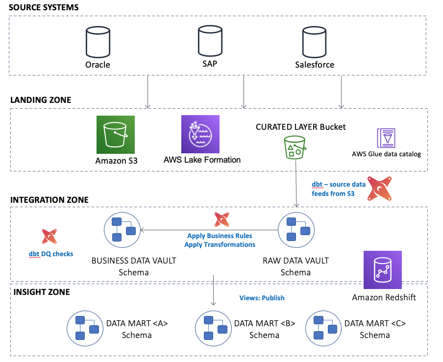
The following diagram illustrates the high-level overview of the architecture:
Amazon Redshift has several methods for ingesting data from Amazon S3 into the data warehouse cluster. For this modern data platform, we use a combination of the following methods:
We use Amazon Redshift Spectrum to read data directly from Amazon S3. This allows the project to rapidly load, store, and use external datasets. Amazon Redshift allows the creation of external schemas and external tables to facilitate data being accessed using standard SQL statements.
Some feeds are persisted in a staging schema within Amazon Redshift, for example larger data volumes and datasets that are used multiple times in subsequent ELT processing. dbt handles the orchestration and loading of this data in an incremental manner to cater to daily delta changes.
Within Amazon Redshift, the Data Vault 2.0 data model is split into three separate areas:
Raw Data Vault within a schema called raw_dv
Business Data Vault within a schema called business_dv
Multiple Data Marts, each with their own schema
Raw Data Vault
Business keys are central to the success of any Data Vault project, and we created hubs within Amazon Redshift as follows:
The business keys from one or more source feeds are written to the reusable _bk column; compound business keys should be concatenated together with a common separator between each element.
The primary key is stored in the _pk column and is a hashed value of the _bk column. In this case, MD5 is the hashing algorithm used.
Load_Dts is the date and time of the insertion of this row.
Hubs hold reference data, which is typically smaller in volume than transactional data, so you should choose a distribution style of ALL for the most performant joining to other tables at runtime.
Because Data Vault is built on a common reusable notation, the dbt code is parameterized for each target. The Roche engineers built a Yaml-driven code framework to parameterize the logic for the build of each target table, enabling rapid build and testing of new feeds. For example, the preceding user hub contains parameters to identify source columns for the business key, source to target mappings, and physicalization choices for the Amazon Redshift target:
On reading the YAML configuration, dbt outputs the following, which is run against the Amazon Redshift cluster:
{# Script generated by dbt model generator #}

{{
	config({
	  "materialized": "incremental",
	  "schema": "raw_dv",
	  "dist": "all",
	  "unique_key": "user_pk",
	  "insert_only": {}
	})
}}

with co_rems_invitee as (

	select
		{{ hash(['dwh_source_country_cd', 'employee_user_id'], 'user_pk') }},
		cast({{ compound_key(['dwh_source_country_cd', 'employee_user_id']) }} as varchar(50)) as user_bk,
		{{ dbt_utils.current_timestamp() }} as load_dts,
		glue_dts as load_source_dts,
		bookmark_dts as bookmark_dts,
		cast('REMS' as varchar(10)) as source_system_cd
	from
		{{ source('re_rems_core', 'co_rems_invitee') }}
	where
		dwh_source_country_cd is not null
		and employee_user_id is not null

		{% if is_incremental() %}
			and glue_dts > (select coalesce(max(load_source_dts), to_date('20000101', 'yyyymmdd', true)) from {{ this }})
		{% endif %}

),
co_rems_event_users as (

	select
		{{ hash(['dwh_source_country_cd', 'user_name'], 'user_pk') }},
		cast({{ compound_key(['dwh_source_country_cd', 'user_name']) }} as varchar(50)) as user_bk,
		{{ dbt_utils.current_timestamp() }} as load_dts,
		glue_dts as load_source_dts,
		bookmark_dts as bookmark_dts,
		cast('REMS' as varchar(10)) as source_system_cd
	from
		{{ source('re_rems_core', 'co_rems_event_users') }}
	where
		dwh_source_country_cd is not null
		and user_name is not null

		{% if is_incremental() %}
			and glue_dts > (select coalesce(max(load_source_dts), to_date('20000101', 'yyyymmdd', true)) from {{ this }})
		{% endif %}

),
all_sources as (

	select * from co_rems_invitee
	union
	select * from co_rems_event_users

),
unique_key as (

	select
		row_number() over(partition by user_pk order by bookmark_dts desc) as rn,
		user_pk,
		user_bk,
		load_dts,
		load_source_dts,
		bookmark_dts,
		source_system_cd
	from
		all_sources

)
select
	user_pk,
	user_bk,
	load_dts,
	load_source_dts,
	bookmark_dts,
	source_system_cd
from
	unique_key
where
	rn = 1
dbt also has the capability to add reusable macros to allow common tasks to be automated. The following example shows the construction of the business key with appropriate separators (the macro is called compound_key):
{% macro single_key(field) %}
  {# Takes an input field value and returns a trimmed version of it. #}
  NVL(NULLIF(TRIM(CAST({{ field }} AS VARCHAR)), ''), '@@')
{% endmacro %}

{% macro compound_key(field_list,sort=none) %}
  {# Takes an input field list and concatenates it into a single column value.
     NOTE: Depending on the sort parameter [True/False] the input field
     list has to be passed in a correct order if the sort parameter
     is set to False (default option) or the list will be sorted
     if You will set up the sort parameter value to True #}
  {% if sort %}
    {% set final_field_list = field_list|sort %}
  {%- else -%}
    {%- set final_field_list = field_list -%}
  {%- endif -%}
  {% for f in final_field_list %}
    {{ single_key(f) }}
    {% if not loop.last %} || '^^' || {% endif %}
  {% endfor %}
{% endmacro %}

{% macro hash(columns=none, alias=none, algorithm=none) %}
    {# Applies a Redshift supported hash function to the input string
       or list of strings. #}

    {# If single column to hash #}
    {% if columns is string %}
        {% set column_str = single_key(columns) %}
        {{ redshift__hash(column_str, alias, algorithm) }}
    {# Else a list of columns to hash #}
    {% elif columns is iterable %}
        {% set column_str = compound_key(columns) %}
        {{ redshift__hash(column_str, alias, algorithm) }}
    {% endif %}

{% endmacro %}

{% macro redshift__hash(column_str, alias, algorithm) %}
    {# Applies a Redshift supported hash function to the input string. #}

    {# If the algorithm is none the default project configuration for hash function will be used. #}
    {% if algorithm == none or algorithm not in ['MD5', 'SHA', 'SHA1', 'SHA2', 'FNV_HASH'] %}
        {# Using MD5 if the project variable is not defined. #}
        {% set algorithm = var('project_hash_algorithm', 'MD5') %}
    {% endif %}

    {# Select hashing algorithm #}
    {% if algorithm == 'FNV_HASH' %}
        CAST(FNV_HASH({{ column_str }}) AS BIGINT) AS {{ alias }}
    {% elif algorithm == 'MD5' %}
        CAST(MD5({{ column_str }}) AS VARCHAR(32)) AS {{ alias }}
    {% elif algorithm == 'SHA' or algorithm == 'SHA1' %}
        CAST(SHA({{ column_str }}) AS VARCHAR(40)) AS {{ alias }}
    {% elif algorithm == 'SHA2' %}
        CAST(SHA2({{ column_str }}, 256) AS VARCHAR(256)) AS {{ alias }}
    {% endif %}

{% endmacro %}
Historized reference data about each business key is stored in satellites. The primary key of each satellite is a compound key consisting of the _pk column of the parent hub and the Load_Dts. See the following code:
The feed name is saved as part of the satellite name. This allows the loading of reference data from either multiple feeds within the same source system or from multiple source systems.
Satellites are insert only; new reference data is loaded as a new row with an appropriate Load_Dts.
The HASH_DIFF column is a hashed concatenation of all the descriptive columns within the satellite. The dbt code uses it to decide whether reference data has changed and a new row is to be inserted.
Unless the data volumes within a satellite become very large (millions of rows), you should choose a distribution choice of ALL to enable the most performant joins at runtime. For larger volumes of data, choose a distribution style of AUTO to take advantage of Amazon Redshift automatic table optimization, which chooses the most optimum distribution style and sort key based on the downstream usage of these tables.
Transactional data is stored in a combination of link and link satellite tables. These tables hold the business keys that contribute to the transaction being undertaken as well as optional measures describing the transaction.
Previously, we showed the build of the user hub and two of its satellites. In the following link table, the user hub foreign key is one of several hub keys in the compound key:
The foreign keys back to each hub are a hash value of the business keys, giving a 1:1 join with the _pk column of each hub.
The primary key of this link table is a hash value of all of the hub foreign keys.
The primary key gives direct access to the optional link satellite that holds further historized data about this transaction. The definition of the link satellites is almost identical to satellites; instead of the _pk from the hub being part of the compound key, the _pk of the link is used.
Because data volumes are typically larger for links and link satellites than hubs or satellites, you can again choose AUTO distribution style to let Amazon Redshift choose the optimum physical table distribution choice. If you do choose a distribution style, then choose KEY on the _pk column for both the distribution style and sort key on both the link and any link satellites. This improves downstream query performance by co-locating the datasets on the same slice within the compute nodes and enables MERGE JOINS at run time for optimum performance.
In addition to the dbt code to build all the preceding targets in the Amazon Redshift schemas, the product contains a powerful testing tool that makes assertions on the underlying data contents. The platform continuously tests the results of each data load.
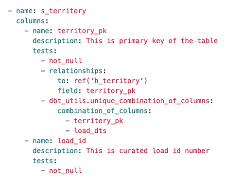
Tests are specified using a YAML file called schema.yml. For example, taking the territory satellite (s_territory), we can see automated testing for conditions, including ensuring the primary key is populated, its parent key is present in the territory hub (h_territory), and the compound key of this satellite is unique:
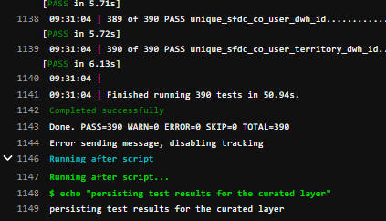
As shown in the following screenshot, the tests are clearly labeled as PASS or FAILED for quick identification of data quality issues.
Business Data Vault
The Business Data Vault is a vital element of any Data Vault model. This is the place where business rules, KPI calculations, performance denormalizations, and roll-up aggregations take place. Business rules can change over time, but the raw data does not, which is why the contents of the Raw Data Vault should never be modified.
The type of objects created in the Business Data Vault schema include the following:
Type 2 denormalization based on either the latest load date timestamp or a business-supplied effective date timestamp. These objects are ideal as the base for a type 2 dimension view within a data mart.
Latest row filtering based on either the latest load date timestamp or a business-supplied effective date timestamp. These objects are ideal as the base for a type 1 dimension within a data mart.
For hubs with multiple independently loaded satellites, point-in-time (PIT) tables are created with the snapshot date set to one time per day.
Where the data access requirements span multiple links and link satellites, bridge tables are created with the snapshot date set to one time per day.
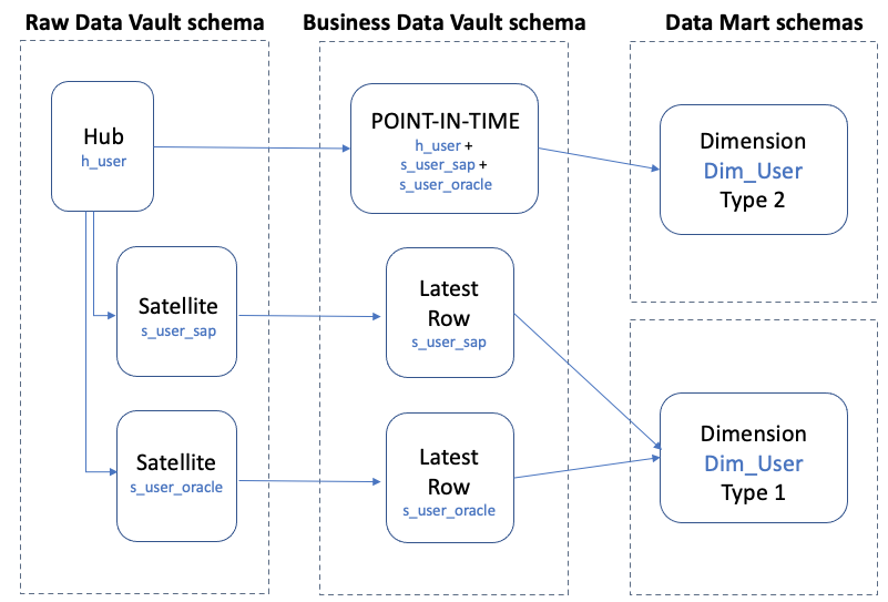
In the following diagram, we show an example of user reference data from two source systems being loaded into separate satellite targets.
Keep in mind the following:
You should create a separate schema for the Business Data Vault objects
You can build several object types in the Business Data Vault:
PIT and bridge targets are typically either tables or materialized views can be used for data that incrementally changes due to the auto refresh capabilities
The type 2 and latest row selections from an underlying satellite are typically views because of the lower data volumes typically found in reference datasets
Because the Raw Data Vault tables are insert only, to determine a timeline of changes, create a view similar to the following:
CREATE OR REPLACE VIEW business_dv.ref_user_type2 AS
SELECT
  s.user_pk,
  s.load_dts from_dts,
  DATEADD(second,-1,COALESCE(LEAD(s.load_dts) OVER (PARTITION BY s.user_pk ORDER BY s.load_dts),'2200-01-01 00:00:00')) AS to_dts
  FROM raw_dv.s_user_reine2 s
  INNER JOIN raw_dv.h_user h ON h.user_pk = s.user_pk
  WITH NO SCHEMA BINDING;
Data Marts
The work undertaken in the Business Data Vault means that views can be developed within the Data Marts to directly access the data without having to physicalize the results into another schema. These views may apply filters to the Business Vault objects, for example to filter only for data from specific countries, or the views may choose a KPI that has been calculated in the Business Vault that is only useful within this one data mart.
Conclusion
In this post, we detailed how you can use dbt and Amazon Redshift for continuous build and validation of a Data Vault model that stores all data from multiple sources in a source-independent manner while offering flexibility and choice of subsequent business transformations and calculations.
Special thanks go to Roche colleagues Bartlomiej Zalewski, Wojciech Kostka, Michalina Mastalerz, Kamil Piotrowski, Igor Tkaczyk, Andrzej Dziabowski, Joao Antunes, Krzysztof Slowinski, Krzysztof Romanowski, Patryk Szczesnowicz, Jakub Lanski, and Chun Wei Chan for their project delivery and support with this post.
About the Authors
Dr. Yannick Misteli, Roche – Dr. Yannick Misteli is leading cloud platform and ML engineering teams in global product strategy (GPS) at Roche. He is passionate about infrastructure and operationalizing data-driven solutions, and he has broad experience in driving business value creation through data analytics.
Simon Dimaline, AWS – Simon Dimaline has specialised in data warehousing and data modelling for more than 20 years. He currently works for the Data & Analytics team within AWS Professional Services, accelerating customers’ adoption of AWS analytics services.
Matt Noyce, AWS – Matt Noyce is a Senior Cloud Application Architect in Professional Services at Amazon Web Services. He works with customers to architect, design, automate, and build solutions on AWS for their business needs.
Chema Artal Banon, AWS – Chema Artal Banon is a Security Consultant at AWS Professional Services and he works with AWS’s customers to design, build, and optimize their security to drive business. He specializes in helping companies accelerate their journey to the AWS Cloud in the most secure manner possible by helping customers build the confidence and technical capability.
The Open Source Security Foundation announced $10 million in funding from a pool of tech and financial companies, including $5 million from Microsoft and Google, to find vulnerabilities in open source projects:
The “Alpha” side will emphasize vulnerability testing by hand in the most popular open-source projects, developing close working relationships with a handful of the top 200 projects for testing each year. “Omega” will look more at the broader landscape of open source, running automated testing on the top 10,000.
This is an excellent idea. This code ends up in all sorts of critical applications.
Log4j would be a prototypical vulnerability that the Alpha team might look for – an unknown problem in a high-impact project that automated tools would not be able to pick up before a human discovered it. The goal is not to use the personnel engaged with Alpha to replicate dependency analysis, for example.
Innovations solve longstanding problems in creative, impactful ways — but they also raise new questions, especially when they’re in the liminal space between being an emerging idea and a fully fledged, widely adopted reality. One of the still-unanswered questions about extended detection and response (XDR) is what its relationship is with security information and event management (SIEM), a more broadly understood and implemented product category that most security teams have already come to rely on.
When looking at the foundations of XDR, it seems like it could be a replacement for, or an alternative to, SIEM. But as Forrester analyst Allie Mellen noted in her recent conversation with Rapid7’s Sam Adams, VP for Detection and Response, the picture isn’t quite that simple.
“Some SIEM vendors are repositioning themselves as XDR,” Allie said, “kind of trying to latch onto that new buzzword.” She added, “The challenge with that is it’s very hard to see what they’re able to offer that’s actually differentiating from SIEM.”
Where SIEM stands today
To really understand how the rise of XDR is impacting SIEM and what relationship we should expect between the two product types, we first need to ask a key question: How are security operations center (SOC) teams actually using their SIEMs today?
At Forrester, Allie recently conducted a survey asking SOC teams this very question. While some have focused on the compliance use case as a main driver for SIEM adoption, Allie found that just wasn’t the case with her survey respondents. Overwhelmingly, security analysts are using their SIEMs for detection and response, making it the core tool within the SOC.
More than that, Allie’s survey actually found the old adage that security teams hate their SIEMs just isn’t true. The vast majority of analysts she surveyed love using their SIEMs (even if they wish it cost them less).
Together, for now
With SIEM claiming such an integral role in the SOC, Allie acknowledged that we likely shouldn’t expect it to be simply replaced by XDR in the near term.
“For the time being, I definitely see XDR and SIEM living together in a very cohesive fashion,” she said.
She went on to suggest that maybe in 5 years or so, we’ll start to see XDR offerings that truly tackle all SIEM use cases and fully deliver on some capabilities that are only in the realm of possibility today. But until XDR can fully address compliance, for example, we’re likely to see it exist alongside and, ideally, in harmony with SIEM.
The XDR opportunity
So, what will that coexistence of SIEM and XDR look like? Sam suggested it might be the fulfillment of the original vision of SIEM solutions like InsightIDR: to make the security analyst superhuman by enabling them to be hyper-efficient at detecting and responding to threats. Allie echoed this sentiment, noting that XDR is all about elevating the role of the SOC analyst rather than automating their tasks away.
“I am not a big believer in the autonomous SOC or this idea that we’re going to take away all the humans from this process,” she said. “At the end of the day, it’s a human-to-human fight. The attackers are not automating themselves away, so it’s very unlikely that we’ll be able to create a product that can keep up with as many human beings as there are attacking us all the time.”
For Allie, the really exciting thing about XDR is its potential to humanize security operations. By reducing the amount of repetitive work analysts have to do, it frees them up to be truly creative and visionary in their threat detection efforts. This can also help improve retention rates among security pros as organizations scramble to fill the cybersecurity skills gap.
“It’s a lofty dream, a lofty vision,” Allie acknowledged, “but XDR is definitely pushing down that path.”
Version 7.3 of the LibreOffice “Community” edition is out.
“In addition to the majority of code commits being focused on
interoperability with Microsoft's proprietary file formats, there is a
wealth of new features targeted at users migrating from Office, to simplify
the transition“.
Security updates have been issued by CentOS (samba), Debian (apache2 and python-django), Fedora (kernel and phpMyAdmin), Mageia (kernel and kernel-linus), openSUSE (samba), Oracle (nginx:1.20 and samba), Red Hat (cryptsetup, java-1.8.0-ibm, kernel, nodejs:14, rpm, and vim), SUSE (kernel, python-Django, python-Django1, and samba), and Ubuntu (cron).
Миналата есен офис на турска банка в България получава по мейл офертите на други банки в страната към едно държавно дружество, подадени в рамки на конкурс за избор на обслужващи…
Often programmers have assumptions that turn out, to their surprise, to be invalid. From my experience this happens a lot. Every API, technology or system can be abused beyond its limits and break in a miserable way.
It’s particularly interesting when basic things used everywhere fail. Recently we’ve reached such a breaking point in a ubiquitous part of Linux networking: establishing a network connection using the connect() system call.
Since we are not doing anything special, just establishing TCP and UDP connections, how could anything go wrong? Here’s one example: we noticed alerts from a misbehaving server, logged in to check it out and saw:
marek@:~# ssh 127.0.0.1
ssh: connect to host 127.0.0.1 port 22: Cannot assign requested address
You can imagine the face of my colleague who saw that. SSH to localhost refuses to work, while she was already using SSH to connect to that server! On another occasion:
marek@:~# dig cloudflare.com @1.1.1.1
dig: isc_socket_bind: address in use
This time a basic DNS query failed with a weird networking error. Failing DNS is a bad sign!
In both cases the problem was Linux running out of ephemeral ports. When this happens it’s unable to establish any outgoing connections. This is a pretty serious failure. It’s usually transient and if you don’t know what to look for it might be hard to debug.
The root cause lies deeper though. We can often ignore limits on the number of outgoing connections. But we encountered cases where we hit limits on the number of concurrent outgoing connections during normal operation.
In this blog post I’ll explain why we had these issues, how we worked around them, and present an userspace code implementing an improved variant of connect() syscall.
Outgoing connections on Linux part 1 – TCP
Let’s start with a bit of historical background.
Long-lived connections
Back in 2014 Cloudflare announced support for WebSockets. We wrote two articles about it:
If you skim these blogs, you’ll notice we were totally fine with the WebSocket protocol, framing and operation. What worried us was our capacity to handle large numbers of concurrent outgoing connections towards the origin servers. Since WebSockets are long-lived, allowing them through our servers might greatly increase the concurrent connection count. And this did turn out to be a problem. It was possible to hit a ceiling for a total number of outgoing connections imposed by the Linux networking stack.
In a pessimistic case, each Linux connection consumes a local port (ephemeral port), and therefore the total connection count is limited by the size of the ephemeral port range.
Basics – how port allocation works
When establishing an outbound connection a typical user needs the destination address and port. For example, DNS might resolve cloudflare.com to the ‘104.1.1.229’ IPv4 address. A simple Python program can establish a connection to it with the following code:
cd = socket.socket(AF_INET, SOCK_STREAM)
cd.connect(('104.1.1.229', 80))
The operating system’s job is to figure out how to reach that destination, selecting an appropriate source address and source port to form the full 4-tuple for the connection:
The operating system chooses the source IP based on the routing configuration. On Linux we can see which source IP will be chosen with ip route get:
$ ip route get 104.1.1.229
104.1.1.229 via 192.168.1.1 dev eth0 src 192.168.1.8 uid 1000
	cache
The src parameter in the result shows the discovered source IP address that should be used when going towards that specific target.
The source port, on the other hand, is chosen from the local port range configured for outgoing connections, also known as the ephemeral port range. On Linux this is controlled by the following sysctls:
The ip_local_port_range sets the low and high (inclusive) port range to be used for outgoing connections. The ip_local_reserved_ports is used to skip specific ports if the operator needs to reserve them for services.
Vanilla TCP is a happy case
The default ephemeral port range contains more than 28,000 ports (60999+1-32768=28232). Does that mean we can have at most 28,000 outgoing connections? That’s the core question of this blog post!
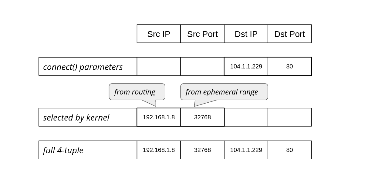
In TCP the connection is identified by a full 4-tuple, for example:
full 4-tuple
192.168.1.8
32768
104.1.1.229
80
In principle, it is possible to reuse the source IP and port, and share them against another destination. For example, there could be two simultaneous outgoing connections with these 4-tuples:
full 4-tuple #A
192.168.1.8
32768
104.1.1.229
80
full 4-tuple #B
192.168.1.8
32768
151.101.1.57
80
This “source two-tuple” sharing can happen in practice when establishing connections using the vanilla TCP code:
But slightly different code can prevent this sharing, as we’ll discuss.
In the rest of this blog post, we’ll summarise the behaviour of code fragments that make outgoing connections showing:
The technique’s description
The typical `errno` value in the case of port exhaustion
And whether the kernel is able to reuse the {source IP, source port}-tuple against another destination
The last column is the most important since it shows if there is a low limit of total concurrent connections. As we’re going to see later, the limit is present more often than we’d expect.
technique description
errno on port exhaustion
possible src 2-tuple reuse
connect(dst_IP, dst_port)
EADDRNOTAVAIL
yes (good!)
In the case of generic TCP, things work as intended. Towards a single destination it’s possible to have as many connections as an ephemeral range allows. When the range is exhausted (against a single destination), we’ll see EADDRNOTAVAIL error. The system also is able to correctly reuse local two-tuple {source IP, source port} for ESTABLISHED sockets against other destinations. This is expected and desired.
Manually selecting source IP address
Let’s go back to the Cloudflare server setup. Cloudflare operates many services, to name just two: CDN (caching HTTP reverse proxy) and WARP.
For Cloudflare, it’s important that we don’t mix traffic types among our outgoing IPs. Origin servers on the Internet might want to differentiate traffic based on our product. The simplest example is CDN: it’s appropriate for an origin server to firewall off non-CDN inbound connections. Allowing Cloudflare cache pulls is totally fine, but allowing WARP connections which contain untrusted user traffic might lead to problems.
To achieve such outgoing IP separation, each of our applications must be explicit about which source IPs to use. They can’t leave it up to the operating system; the automatically-chosen source could be wrong. While it’s technically possible to configure routing policy rules in Linux to express such requirements, we decided not to do that and keep Linux routing configuration as simple as possible.
Instead, before calling connect(), our applications select the source IP with the bind() syscall. A trick we call “bind-before-connect”:
This code looks rather innocent, but it hides a considerable drawback. When calling bind(), the kernel attempts to find an unused local two-tuple. Due to BSD API shortcomings, the operating system can’t know what we plan to do with the socket. It’s totally possible we want to listen() on it, in which case sharing the source IP/port with a connected socket will be a disaster! That’s why the source two-tuple selected when calling bind() must be unique.
Due to this API limitation, in this technique the source two-tuple can’t be reused. Each connection effectively “locks” a source port, so the number of connections is constrained by the size of the ephemeral port range. Notice: one source port is used up for each connection, no matter how many destinations we have. This is bad, and is exactly the problem we were dealing with back in 2014 in the WebSockets articles mentioned above.
Fortunately, it’s fixable.
IP_BIND_ADDRESS_NO_PORT
Back in 2014 we fixed the problem by setting the SO_REUSEADDR socket option and manually retrying bind()+ connect() a couple of times on error. This worked ok, but later in 2015 Linux introduced a proper fix: the IP_BIND_ADDRESS_NO_PORT socket option. This option tells the kernel to delay reserving the source port:
This gets us back to the desired behavior. On modern Linux, when doing bind-before-connect for TCP, you should set IP_BIND_ADDRESS_NO_PORT.
Explicitly selecting a source port
Sometimes an application needs to select a specific source port. For example: the operator wants to control full 4-tuple in order to debug ECMP routing issues.
Recently a colleague wanted to run a cURL command for debugging, and he needed the source port to be fixed. cURL provides the --local-port option to do this¹ :
In other situations source port numbers should be controlled, as they can be used as an input to a routing mechanism.
But setting the source port manually is not easy. We’re back to square one in our hackery since IP_BIND_ADDRESS_NO_PORT is not an appropriate tool when calling bind() with a specific source port value. To get the scheme working again and be able to share source 2-tuple, we need to turn to SO_REUSEADDR:
Here, the user takes responsibility for handling conflicts, when an ESTABLISHED socket sharing the 4-tuple already exists. In such a case connect will fail with EADDRNOTAVAIL and the application should retry with another acceptable source port number.
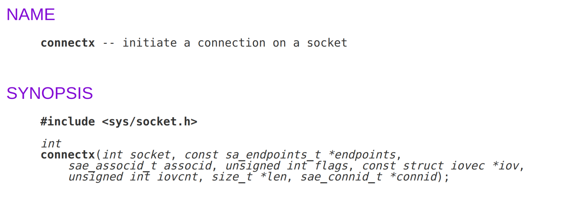
Userspace connectx implementation
With these tricks, we can implement a common function and call it connectx. It will do what bind()+connect() should, but won’t have the unfortunate ephemeral port range limitation. In other words, created sockets are able to share local two-tuples as long as they are going to distinct destinations:
The name we chose isn’t an accident. MacOS (specifically the underlying Darwin OS) has exactly that function implemented as a connectx() system call (implementation):
It’s more powerful than our connectx code, since it supports TCP Fast Open.
Should we, Linux users, be envious? For TCP, it’s possible to get the right kernel behaviour with the appropriate setsockopt/bind/connect dance, so a kernel syscall is not quite needed.
But for UDP things turn out to be much more complicated and a dedicated syscall might be a good idea.
Outgoing connections on Linux – part 2 – UDP
In the previous section we listed three use cases for outgoing connections that should be supported by the operating system:
Vanilla egress: operating system chooses the outgoing IP and port
Source IP selection: user selects outgoing IP but the OS chooses port
Full 4-tuple: user selects full 4-tuple for the connection
We demonstrated how to implement all three cases on Linux for TCP, without hitting connection count limits due to source port exhaustion.
It’s time to extend our implementation to UDP. This is going to be harder.
For UDP, Linux maintains one hash table that is keyed on local IP and port, which can hold duplicate entries. Multiple UDP connected sockets can not only share a 2-tuple but also a 4-tuple! It’s totally possible to have two distinct, connected sockets having exactly the same 4-tuple. This feature was created for multicast sockets. The implementation was then carried over to unicast connections, but it is confusing. With conflicting sockets on unicast addresses, only one of them will receive any traffic. A newer connected socket will “overshadow” the older one. It’s surprisingly hard to detect such a situation. To get UDP connectx() right, we will need to work around this “overshadowing” problem.
Vanilla UDP is limited
It might come as a surprise to many, but by default, the total count for outbound UDP connections is limited by the ephemeral port range size. Usually, with Linux you can’t have more than ~28,000 connected UDP sockets, even if they point to multiple destinations.
Ok, let’s start with the simplest and most common way of establishing outgoing UDP connections:
The simplest case is not a happy one. The total number of concurrent outgoing UDP connections on Linux is limited by the ephemeral port range size. On our multi-tenant servers, with potentially long-lived gaming and H3/QUIC flows containing WebSockets, this is too limiting.
On TCP we were able to slap on a setsockopt and move on. No such easy workaround is available for UDP.
For UDP, without REUSEADDR, Linux avoids sharing local 2-tuples among UDP sockets. During connect() it tries to find a 2-tuple that is not used yet. As a side note: there is no fundamental reason that it looks for a unique 2-tuple as opposed to a unique 4-tuple during ‘connect()’. This suboptimal behavior might be fixable.
SO_REUSEADDR is hard
To allow local two-tuple reuse we need the SO_REUSEADDR socket option. Sadly, this would also allow established sockets to share a 4-tuple, with the newer socket overshadowing the older one.
In other words, we can’t just set SO_REUSEADDR and move on, since we might hit a local 2-tuple that is already used in a connection against the same destination. We might already have an identical 4-tuple connected socket underneath. Most importantly, during such a conflict we won’t be notified by any error. This is unacceptably bad.
Detecting socket conflicts with eBPF
We thought a good solution might be to write an eBPF program to detect such conflicts. The idea was to put a code on the connect() syscall. Linux cgroups allow the BPF_CGROUP_INET4_CONNECT hook. The eBPF is called every time a process under a given cgroup runs the connect() syscall. This is pretty cool, and we thought it would allow us to verify if there is a 4-tuple conflict before moving the socket from UNCONNECTED to CONNECTED states.
However, this solution is limited. First, it doesn’t work for sockets with an automatically assigned source IP or source port, it only works when a user manually creates a 4-tuple connection from userspace. Then there is a second issue: a typical race condition. We don’t grab any lock, so it’s technically possible a conflicting socket will be created on another CPU in the time between our eBPF conflict check and the finish of the real connect() syscall machinery. In short, this lockless eBPF approach is better than nothing, but fundamentally racy.
Socket traversal – SOCK_DIAG ss way
There is another way to verify if a conflicting socket already exists: we can check for connected sockets in userspace. It’s possible to do it without any privileges quite effectively with the SOCK_DIAG_BY_FAMILY feature of netlink interface. This is the same technique the ss tool uses to print out sockets available on the system.
This code has the same race condition issue as the connect inet eBPF hook before. But it’s a good starting point. We need some locking to avoid the race condition. Perhaps it’s possible to do it in the userspace.
SO_REUSEADDR as a lock
Here comes a breakthrough: we can use SO_REUSEADDR as a locking mechanism. Consider this:
We need REUSEADDR around bind, otherwise it wouldn’t be possible to reuse a local port. It’s technically possible to clear REUSEADDR after bind. Doing this technically makes the kernel socket state inconsistent, but it doesn’t hurt anything in practice.
By clearing REUSEADDR, we’re locking new sockets from using that source port. At this stage we can check if we have ownership of the 4-tuple we want. Even if multiple sockets enter this critical section, only one, the newest, can win this verification. This is a cooperative algorithm, so we assume all tenants try to behave.
At this point, if the verification succeeds, we can perform connect() and have a guarantee that the 4-tuple won’t be reused by another socket at any point in the process.
This is rather convoluted and hacky, but it satisfies our requirements:
technique description
errno on port exhaustion
possible src 2-tuple reuse
risk of overshadowing
REUSEADDR as a lock
EAGAIN
yes
no
Sadly, this schema only works when we know the full 4-tuple, so we can’t rely on kernel automatic source IP or port assignments.
Faking source IP and port discovery
In the case when the user calls ‘connect’ and specifies only target 2-tuple – destination IP and port, the kernel needs to fill in the missing bits – the source IP and source port. Unfortunately the described algorithm expects the full 4-tuple to be known in advance.
One solution is to implement source IP and port discovery in userspace. This turns out to be not that hard. For example, here’s a snippet of our code:
def _get_udp_port(family, src_addr, dst_addr):
    if ephemeral_lo == None:
        _read_ephemeral()
    lo, hi = ephemeral_lo, ephemeral_hi
    start = random.randint(lo, hi)
    ...
Putting it all together
Combining the manual source IP, port discovery and the REUSEADDR locking dance, we get a decent userspace implementation of connectx() for UDP.
We have covered all three use cases this API should support:
This post described a problem we hit in production: running out of ephemeral ports. This was partially caused by our servers running numerous concurrent connections, but also because we used the Linux sockets API in a way that prevented source port reuse. It meant that we were limited to ~28,000 concurrent connections per protocol, which is not enough for us.
We explained how to allow source port reuse and prevent having this ephemeral-port-range limit imposed. We showed an userspace connectx() function, which is a better way of creating outgoing TCP and UDP connections on Linux.
Our UDP code is more complex, based on little known low-level features, assumes cooperation between tenants and undocumented behaviour of the Linux operating system. Using REUSEADDR as a locking mechanism is rather unheard of.
The connectx() functionality is valuable, and should be added to Linux one way or another. It’s not trivial to get all its use cases right. Hopefully, this blog post shows how to achieve this in the best way given the operating system API constraints.
___
¹ On a side note, on the second cURL run it fails due to TIME-WAIT sockets: “bind failed with errno 98: Address already in use”.
One option is to wait for the TIME_WAIT socket to die, or work around this with the time-wait sockets kill script. Killing time-wait sockets is generally a bad idea, violating protocol, unneeded and sometimes doesn’t work. But hey, in some extreme cases it’s good to know what’s possible. Just saying.
The problem of how to deprecate pieces of the Python language
in a minimally disruptive way has cropped in various guises over the last few years—in truth,
it has been wrangled with throughout much of language’s 30-year history.
The scars of the biggest deprecation, that of Python 2, are still rather
fresh, both for users and the core developers, so no one wants (or plans)
a monumental change of that sort. But the language community does want to
continue evolving Python, which means leaving some “baggage” behind; how
to do so without leaving further scars is a delicate balancing act, as yet
another discussion highlights.
To provide the best experiences, we use technologies like cookies to store and/or access device information. Consenting to these technologies will allow us to process data such as browsing behavior or unique IDs on this site. Not consenting or withdrawing consent, may adversely affect certain features and functions.
Functional
Always active
The technical storage or access is strictly necessary for the legitimate purpose of enabling the use of a specific service explicitly requested by the subscriber or user, or for the sole purpose of carrying out the transmission of a communication over an electronic communications network.
Preferences
The technical storage or access is necessary for the legitimate purpose of storing preferences that are not requested by the subscriber or user.
Statistics
The technical storage or access that is used exclusively for statistical purposes.The technical storage or access that is used exclusively for anonymous statistical purposes. Without a subpoena, voluntary compliance on the part of your Internet Service Provider, or additional records from a third party, information stored or retrieved for this purpose alone cannot usually be used to identify you.
Marketing
The technical storage or access is required to create user profiles to send advertising, or to track the user on a website or across several websites for similar marketing purposes.
![[Security Nation] John Rouffas on Building a Security Function](https://blog.rapid7.com/content/images/2022/02/John-Rouffas-bio-_1_.jpg)