As of this writing, Linus Torvalds has pulled exactly 6,800 non-merge
changesets into the mainline repository for the 5.16 kernel release. That
is probably a little over half of what will arrive during this merge
window, so this is a good time to catch up on what has been pulled so far.
There are many significant changes and some large-scale restructuring of
internal kernel code, but relatively few ground-breaking new
features.
Security updates have been issued by Fedora (ansible, chromium, kernel, mupdf, python-PyMuPDF, rust, and zathura-pdf-mupdf), openSUSE (qemu and webkit2gtk3), Red Hat (firefox and kpatch-patch), Scientific Linux (firefox), SUSE (qemu, tomcat, and webkit2gtk3), and Ubuntu (firefox and thunderbird).
In this special bonus episode of Security Nation, Jen and Tod chat with Pete Cooper and Irene Pontisso from the UK Cabinet Office about their current competition aiming to promote cybersecurity culture among small businesses. They highlight their 9 hypotheses, which touch on the role of human factors, the distinction between cyber culture and security culture, and the importance of leadership. They chat about why they decided to get help validating these ideas through a competition format — the “Bakeoff Approach,” as Irene calls — to promote collaborative thinking and get a sense of what organizations are doing on these issues today.
The deadline to apply for the competition is fast approaching on Monday, November 8, and winners will be awarded contracts to carry out the competition over 12 weeks, beginning in late November. Check out the Invitation to Tender to submit your entry!
Pete Cooper
Pete Cooper is Deputy Director Cyber Defence within the Government Security Group in the UK Cabinet Office, where he looks over the whole of the Government sector and is responsible for the Government Cyber Security Strategy, standards, and policies as well as responding to serious or cross-government cyber incidents. With a diverse military, private-sector, and government background, he has worked on everything ranging from cyber operations, global cyber security strategies, advising on the nature of state-vs.-state cyber conflict to leading cybersecurity change across industry, public sector, and the global hacker community, including founding and leading the Aerospace Village at DEF CON. A fast jet pilot turned cyber operations advisor, who on leaving the military in 2016, founded the UK’s first multi-disciplinary cyber strategy competition, he is passionate about tackling national and international cybersecurity challenges through better collaboration, diversity, and innovative partnerships. He has a Post Grad in Cyberspace Operations from Cranfield University, is a Non-Resident Senior Fellow at the Cyber Statecraft Initiative of the Scowcroft Centre for Strategy and Security at the Atlantic Council, and is a Visiting Senior Research Fellow in the Department of War Studies, King’s College London.
Irene Pontisso
Irene is Assistant Head of Engagement and Information within the Government Security Group in the UK Cabinet Office. Irene is responsible for the design and strategic oversight of cross-government security education, awareness, and culture-related initiatives. She is also responsible for leading cross-government engagement and press activities for Government Security and the Government Chief Security Officer. Irene started her career in policy and international relations through her roles at the United Nations Platform for Space-Based Information for Disaster Management and Emergency Response (UN-SPIDER). Irene also has significant industry and third-sector experience, and she partnered with the world’s leading law firms to provide free access to legal advice for NGOs on international development projects. She also has experience in leading large-scale exhibitions and policy research in corporate environments. She holds a MSc in International Relations from the University of Bristol and a BSc from the University of Turin.
Like the show? Want to keep Jen and Tod in the podcasting business? Feel free to rate and review with your favorite podcast purveyor, like Apple Podcasts.
Want More Inspiring Stories From the Security Community?
MITRE ATT&CK is considered by practitioners and the analyst community to be the most comprehensive framework of cybersecurity attacks and mitigation techniques available today. MITRE helps the security industry speak the same language and stick to a well-known, common framework.
To get more details on MITRE’s ATT&CK Matrix for Enterprise and its impact, I spoke with 3 members of Rapid7’s Managed Detection and Response team who have firsthand experience working with this framework every day — read our conversation below!
Laying some groundwork here, what are your thoughts on the MITRE ATT&CK framework?
John Fenninger, Manager of Rapid7’s Detection and Response Services, kicked us off by sharing his perspective:
“MITRE ATT&CK is an incredibly valuable framework for both vendors and customers. From things like compliance to more immediate needs like investigating an ongoing attack, MITRE makes it easy to see specific techniques that customers may not have heard of and helps think of tactical moves customers can protect against. With InsightIDR specifically, we align our detections to MITRE to give both our MDR SOC analysts and customers visibility into how far along a threat is on the ATT&CK chain.”
Rapid7 is not only a consumer of the MITRE ATT&CK Framework but an active contributor as well — in 2020, Rapid7 Incident Response Consultant Ted Samuels made a contribution to MITRE around a discovery for group policy objects that is now in the latest version of the ATT&CK framework.
Can you share your perspective on how the MITRE framework is used, and by who?
When it comes to leveraging the MITRE ATT&CK framework, there are 2 key audiences to consider, says Rapid7’s Senior Detection & Response Analyst, Vidya Tambe:
“There are 2 main categories of users — people who write detections and people who do the analysis of the detections, and the MITRE framework is important for both. From the analyst side, we want to know what stage of attack each alert is at, and based on where the alert falls, we know how critical an incident is. With MITRE, we can track how an attacker got to where they are and what kind of escalations they did — overall, it helps us back-track to see what they were able to compromise.
“From the detection writing standpoint, we want to stop attacks before they get too far into someone’s environment. Attacker techniques are always evolving, and while we aim to write detections for all the phases, a primary focus is to try and write detections early on to stop attackers as early in the ATT&CK chain as possible.”
What advice do you have for security teams when it comes to leveraging the MITRE framework to drive successful detection and response?
Rapid7 Detection and Response Analyst Carlo Anez Mazurco shared some advice for teams when it comes to using the MITRE framework at their organization:
“The MITRE Framework allows us to build a threat-informed defense. It shows us the 3 main areas that we need to focus on for data collection, data analysis, and expansion of detections. For teams to successfully utilize the MITRE framework, they need visibility into the following data sources at a minimum:
Process and process command line monitoring can be collected via Sysmon, Windows Event Logs, and many EDR platforms
File and registry monitoring is also often collected by Sysmon, Windows Event Logs, and many EDR platforms
Authentication logs collected from the domain controller
Packet capture, especially east/west capture, such as those collected between hosts and enclaves in your network
“Teams need a platform like InsightIDR, Rapid7’s extended detection and response solution, where the data from all of these sources can be ingested. Whatever platform or tool teams choose to use for this data ingestion should include MITRE mappings to attacker behaviors to understand what attackers are trying to do inside our environment at each stage, the TTPs (Tactics, Techniques, Procedures) of each threat actor should be documented in each alert — InsightIDR maps its detections to the MITRE framework to do just this for users.”
You mentioned InsightIDR has MITRE mapping — can you dig a little more into how this impacts customers?
“Our InsightIDR platform helps our customers collect all the necessary data sources,” Carlo continued. “That includes process and process command line monitoring via our endpoint Insight Agent, as well as file monitoring. Plus, authentication logs are collected from domain controllers and also via the Insight Agent, and network flow inside the environment can be gathered through our Insight Network Sensor.
“Our ABA and UBA detections are mapped to the MITRE framework to show our customers which TTPs are the most commonly used by threat actors in their environment, and it gives an insight into the attack patterns in real time. You can see an example of this in one of our past Rapid7 Threat Reports here.
“Additionally, our Rapid7 Threat Intelligence team is always developing new threat detections based on the threat intelligence feeds and public repositories of attacker behaviors. These new detections are mapped to the TTPs inside the MITRE framework and pushed out to all Rapid7 customers.”
We also recently released a new view of Detection Rules in InsightIDR where all detections are mapped to the MITRE ATT&CK Framework, and users can see associated MITRE tactics, techniques, and sub-techniques for detections while performing an investigation.
Interested in learning more?
As you can see, we really value the MITRE ATT&CK framework here at Rapid7. With InsightIDR your detections are vetted by a team of professional SOC analysts and mapped to MITRE to take the guessing game of what an attacker might do next.
If you’re looking to hear more from us on MITRE, watch a quick 3-minute rundown on the framework here.
Here’s a summary of the trends observed in Q3 ‘21:
Application-layer (L7) DDoS attack trends:
For the second consecutive quarter in 2021, US-based companies were the most targeted in the world.
For the first time in 2021, attacks on UK-based and Canada-based companies skyrocketed, making them the second and third most targeted countries, respectively.
Attacks on Computer Software, Gaming/ Gambling, IT, and Internet companies increased by an average of 573% compared to the previous quarter.
Meris, one of the most powerful botnets in history, aided in launching DDoS campaigns across various industries and countries. You can read more on that here.
Network-layer (L3/4) DDoS attack trends:
DDoS attacks increased by 44% worldwide compared to the previous quarter.
The Middle East and Africa recorded the largest average attack increase of approximately 80%.
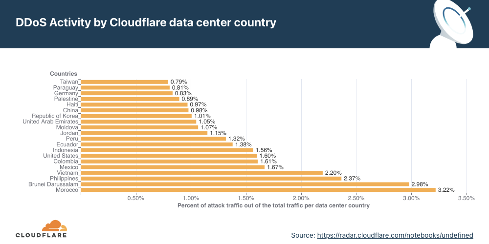
Morocco recorded the highest DDoS activity in the third quarter globally — three out of every 100 packets were part of a DDoS attack.
While SYN and RST attacks remain the dominant attack method used by attackers, Cloudflare observed a surge in DTLS amplification attacks — recording a 3,549% increase QoQ.
Attackers targeted (and continue to target going into the fourth quarter this year) VoIP service providers with massive DDoS attack campaigns in attempts to bring SIP infrastructure down.
Note on avoiding data biases: When we analyze attack trends, we calculate the “DDoS activity” rate, which is the percentage of attack traffic of the total traffic (attack + clean). When reporting application- and network-layer DDoS attack trends, we use this metric, which allows us to normalize the data points and avoid biases toward, for example, a larger Cloudflare data center that naturally handles more traffic and therefore also, possibly, more attacks compared to a smaller Cloudflare data center located elsewhere.
Application-layer DDoS attacks
Application-layer DDoS attacks, specifically HTTP DDoS attacks, are attacks that usually aim to disrupt a web server by making it unable to process legitimate user requests. If a server is bombarded with more requests than it can process, the server will drop legitimate requests and — in some cases — crash, resulting in degraded performance or an outage for legitimate users.
Q3 ‘21 was the quarter of Meris — one of the most powerful botnets deployed to launch some of the largest HTTP DDoS attacks in history.
This past quarter, we observed one of the largest recorded HTTP attacks — 17.2M rps (requests per second) — targeting a customer in the financial services industry. One of the most powerful botnets ever observed, called Meris, is known to be deployed in launching these attacks.
Meris (Latvian for plague) is a botnet behind recent DDoS attacks that have targeted networks or organizations around the world. The Meris botnet infected routers and other networking equipment manufactured by the Latvian company MikroTik. According to MikroTik’s blog, a vulnerability in the MikroTik RouterOS (that was patched after its detection back in 2018) was exploited in still unpatched devices to build a botnet and launch coordinated DDoS attacks by bad actors.
Similar to the Mirai botnet of 2016, Meris is one of the most powerful botnets recorded. While Mirai infected IoT devices with low computational power such as smart cameras, Meris is a growing swarm of networking infrastructure (such as routers and switches) with significantly higher processing power and data transfer capabilities than IoT devices — making them much more potent in causing harm at a larger scale. Be that as it may, Meris is an example of how the attack volume doesn’t necessarily guarantee damage to the target. As far as we know, Meris, despite its strength, was not able to cause significant impact or Internet outages. On the other hand, by tactically targeting the DYN DNS service in 2016, Mirai succeeded in causing significant Internet disruptions.
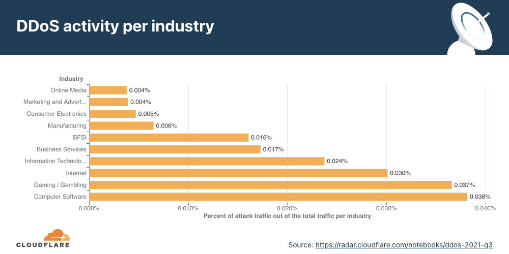
Application-layer DDoS attacks by industry
The tech and gaming industries were the most targeted industries in Q3 ‘21.
When we break down the application-layer attacks targeted by industry, Computer Software companies topped the charts. The Gaming/Gambling industry, also known to be regular targets of online attacks, was a close second, followed by the Internet and IT industries.
Application-layer DDoS attacks by source country
To understand the origin of the HTTP attacks, we look at the geolocation of the source IP address belonging to the client that generated the attack HTTP requests. Unlike network-layer attacks, source IPs cannot be spoofed in HTTP attacks. A high DDoS activity rate in a given country usually indicates the presence of botnets operating from within.
In the third quarter of 2021, most attacks originated from devices/servers in China, the United States, and India. While China remains in first place, the number of attacks originating from Chinese IPs actually decreased by 30% compared to the previous quarter. Almost one out of every 200 HTTP requests that originated from China was part of an HTTP DDoS attack.
Additionally, attacks from Brazil and Germany shrank by 38% compared to the previous quarter. Attacks originating from the US and Malaysia reduced by 40% and 45%, respectively.
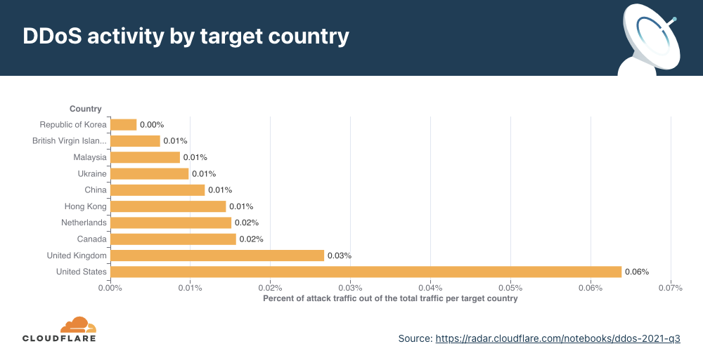
Application-layer DDoS attacks by target country
In order to identify which countries are targeted the most by L7 attacks, we break down the DDoS activity by our customers’ billing countries.
For the second consecutive time this year, organizations in the United States were targeted the most by L7 DDoS attacks in the world, followed by those in the UK and Canada.
Network-layer DDoS attacks
While application-layer attacks target the application (Layer 7 of the OSI model) running the service that end users are trying to access, network-layer attacks aim to overwhelm network infrastructure (such as in-line routers and servers) and the Internet link itself.
Mirai-variant botnet strikes with a force of 1.2 Tbps.
Q3 ‘21 was also the quarter when the infamous Mirai made a resurgence. A Mirai-variant botnet launched over a dozen UDP- and TCP-based DDoS attacks that peaked multiple times above 1 Tbps, with a max peak of approximately 1.2 Tbps. These network-layer attacks targeted Cloudflare customers on the Magic Transit and Spectrum services. One of these targets was a major APAC-based Internet services, telecommunications, and hosting provider and the other was a gaming company. In all cases, the attacks were automatically detected and mitigated without human intervention.
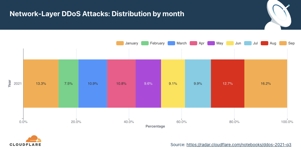
Network-layer DDoS attacks by month
September was, by far, the busiest month for attackers this year.
Q3 ‘21 accounted for more than 38% of all attacks this year. September was the busiest month for attackers so far in 2021 — accounting for over 16% of all attacks this year.
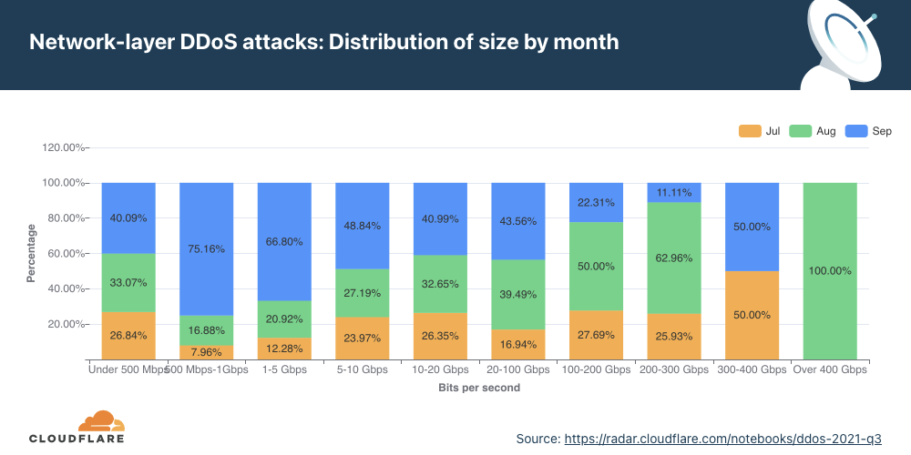
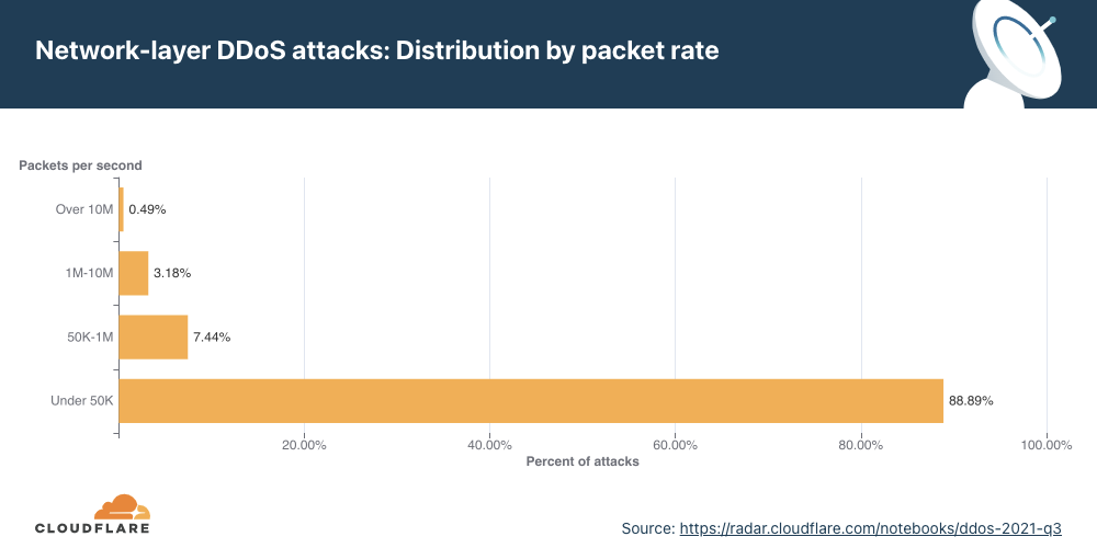
Network-layer DDoS attacks by attack rate
Most attacks are ‘small’ in size, but the number of larger attacks continues to rise.
There are different ways of measuring the size of a L3/4 DDoS attack. One is the volume of traffic it delivers, measured as the bit rate (specifically, terabits per second or gigabits per second). Another is the number of packets it delivers, measured as the packet rate (specifically, millions of packets per second).
Attacks with high bit rates attempt to cause a denial-of-service event by clogging the Internet link, while attacks with high packet rates attempt to overwhelm the servers, routers, or other in-line hardware appliances. Appliances dedicate a certain amount of memory and computation power to process each packet. Therefore, by bombarding it with many packets, the appliance can be left with no further processing resources. In such a case, packets are “dropped,” i.e., the appliance is unable to process them. For users, this results in service disruptions and denial of service.
The distribution of attacks by their size (in bit rate) and month is shown below. Interestingly enough, all attacks over 400 Gbps took place in August, including some of the largest attacks we have seen; multiple attacks peaked above 1 Tbps and reached as high as 1.2 Tbps.
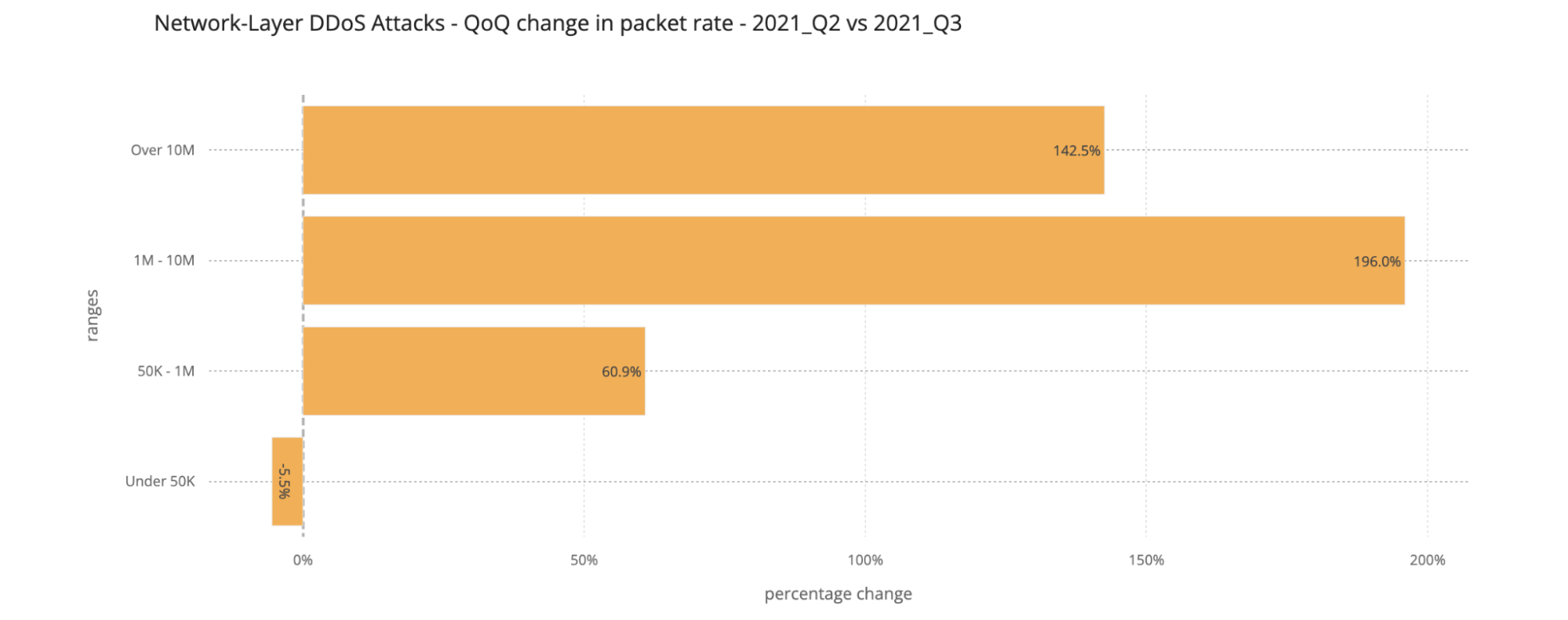
Packet rate As seen in previous quarters, the majority of attacks observed in Q3 ‘21 were relatively small in size — nearly 89% of all attacks peaked below 50K packets per second (pps). While a majority of attacks are smaller in size, we observed that the number of larger attacks is increasing QoQ — attacks that peaked above 10M pps increased by 142% QoQ.
Attacks of packet rates ranging from 1-10 million packets per second increased by 196% compared to the previous quarter. This trend is similar to what we observed the last quarter as well, suggesting that larger attacks are increasing.
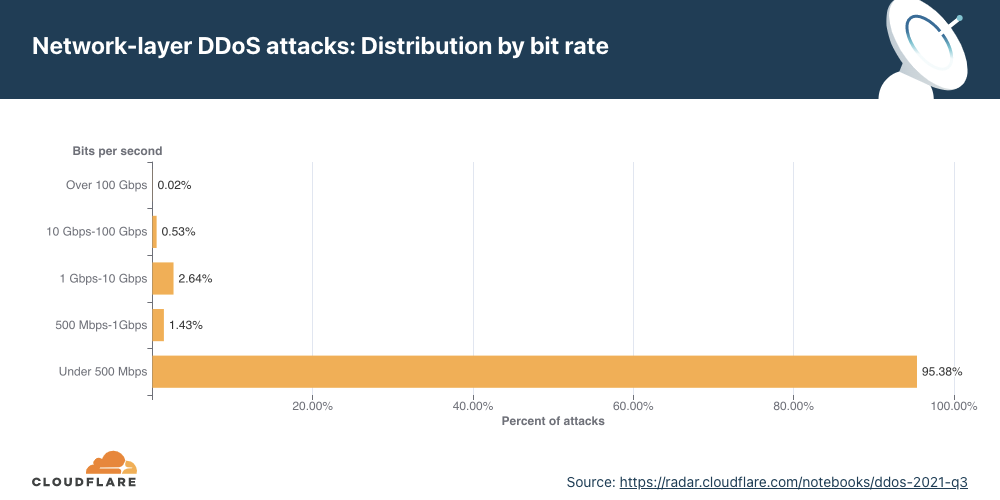
Bit rate From the bit rate perspective, a similar trend was observed — a total of 95.4% of all attacks peaked below 500 Mbps.
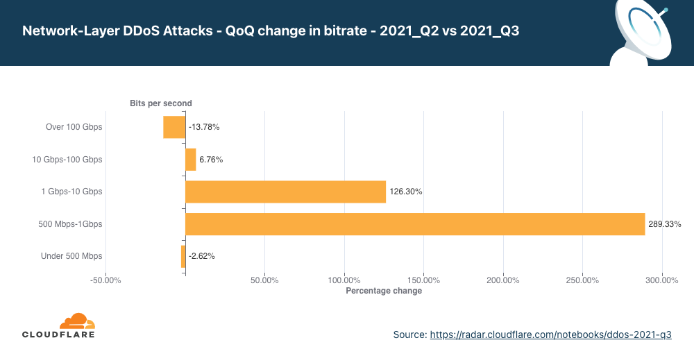
QoQ data shows that the number of attacks of sizes ranging from 500 Mbps to 10 Gbps saw massive increases of 126% to 289% compared to the previous quarter. Attacks over 100 Gbps decreased by nearly 14%.
The number of larger bitrate attacks increased QoQ (with the one exception being attacks over 100 Gbps, which decreased by nearly 14% QoQ). In particular, attacks ranging from 500 Mbps to 1 Gbps saw a surge of 289% QoQ and those ranging from 1 Gbps to 100 Gbps surged by 126%.
This trend once again illustrates that, while (in general) a majority of the attacks are indeed smaller, the number of “larger” attacks is increasing. This suggests that more attackers are garnering more resources to launch larger attacks.
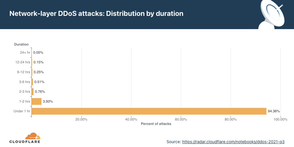
Network-layer DDoS attacks by duration
Most attacks remain under one hour in duration, reiterating the need for automated always-on DDoS mitigation solutions.
We measure the duration of an attack by recording the difference between when it is first detected by our systems as an attack and the last packet we see with that attack signature. As in previous quarters, most of the attacks are short-lived. To be specific, 94.4% of all DDoS attacks lasted less than an hour. On the other end of the axis, attacks over 6 hours accounted for less than 0.4% in Q3 ‘21, and we did see a QoQ increase of 165% in attacks ranging 1-2 hours. Be that as it may, a longer attack does not necessarily mean a more dangerous one.
Short attacks can easily go undetected, especially burst attacks that, within seconds, bombard a target with a significant number of packets, bytes, or requests. In this case, DDoS protection services that rely on manual mitigation by security analysis have no chance in mitigating the attack in time. They can only learn from it in their post-attack analysis, then deploy a new rule that filters the attack fingerprint and hope to catch it next time. Similarly, using an “on-demand” service, where the security team will redirect traffic to a DDoS provider during the attack, is also inefficient because the attack will already be over before the traffic routes to the on-demand DDoS provider.
Cloudflare recommends that companies use automated, always-on DDoS protection services that analyze traffic and apply real-time fingerprinting fast enough to block the short-lived attacks. Cloudflare analyzes traffic out-of-path, ensuring that DDoS mitigation does not add any latency to legitimate traffic, even in always-on deployments. Once an attack is identified, our autonomous edge DDoS protection system (dosd) generates and applies a dynamically crafted rule with a real-time signature. Pre-configured firewall rules comprising allow/deny lists for known traffic patterns take effect immediately.
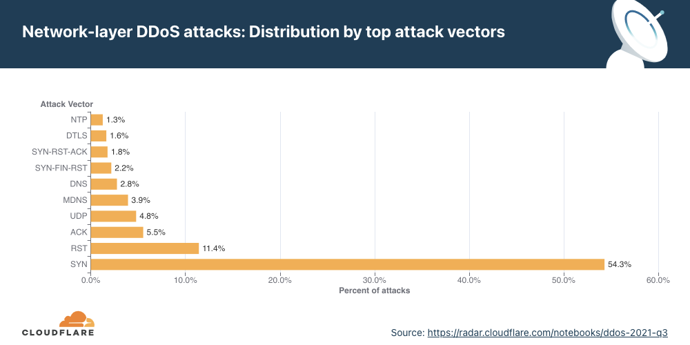
Attack vectors
SYN floods remain attackers’ favorite method of attack, while attacks over DTLS saw a massive surge — 3,549% QoQ.
An attack vector is the term used to describe the method that the attacker utilizes in their attempt to cause a denial-of-service event.
As observed in previous quarters, attacks utilizing SYN floods remain the most popular method used by attackers.
A SYN flood attack is a DDoS attack that works by exploiting the very foundation of the TCP protocol — the stateful TCP connection between a client and a server as a part of the 3-way TCP handshake. As a part of the TCP handshake, the client sends an initial connection request packet with a synchronize flag (SYN). The server responds with a packet that contains a synchronized acknowledgment flag (SYN-ACK). Finally, the client responds with an acknowledgment (ACK) packet. At this point, a connection is established and data can be exchanged until the connection is closed. This stateful process can be abused by attackers to cause denial-of-service events.
By repeatedly sending SYN packets, the attacker attempts to overwhelm a server or the router’s connection table that tracks the state of TCP connections. The server replies with a SYN-ACK packet, allocates a certain amount of memory for each given connection, and falsely waits for the client to respond with the final ACK. Given a sufficient number of connections occupying the server’s memory, the server is unable to allocate further memory for legitimate clients, causing the server to crash or preventing it from handling legitimate client connections, i.e., a denial-of-service event.
More than half of all attacks observed over our network were SYN floods. This was followed by RST, ACK, and UDP floods.
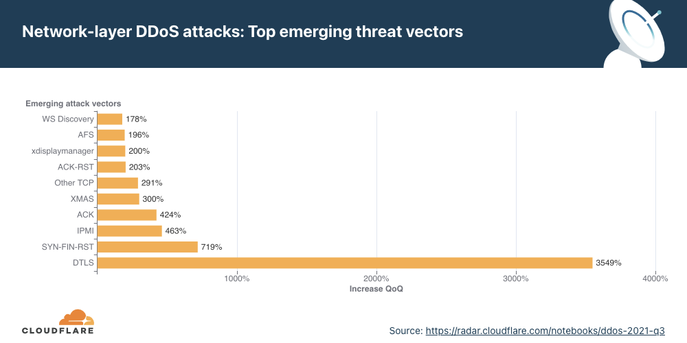
Emerging threats
While SYN and RST floods remain popular overall, when we look at emerging attack vectors — which helps us understand what new vectors attackers are deploying to launch attacks — we observed a massive spike in DTLS amplification attacks. DTLS floods increased by 3,549% QoQ.
Datagram Transport Layer Security (DTLS) is a protocol similar to Transport Layer Security (TLS) designed to provide similar security guarantees to connectionless datagram-based applications to prevent message forgery, eavesdropping, or tampering. DTLS, being connectionless, is specifically useful for establishing VPN connections, without the TCP meltdown problem. The application is responsible for reordering and other connection properties.
Just as with most UDP-based protocols, DTLS is spoofable and being used by attackers to generate reflection amplification attacks to overwhelm network gateways.
Network-layer DDoS attacks by country
While Morocco topped the charts in terms of the highest network attack rate observed, Asian countries closely followed.
When analyzing network-layer DDoS attacks, we bucket the traffic by the Cloudflare edge data center locations where the traffic was ingested, and not by the source IP. The reason for this is that, when attackers launch network-layer attacks, they can spoof the source IP address in order to obfuscate the attack source and introduce randomness into the attack properties, which may make it harder for simple DDoS protection systems to block the attack. Hence, if we were to derive the source country based on a spoofed source IP, we would get a spoofed country.
Cloudflare is able to overcome the challenges of spoofed IPs by displaying the attack data by the location of the Cloudflare data center in which the attack was observed. We are able to achieve geographical accuracy in our report because we have data centers in over 250 cities around the world.
A note on recent attacks on voice over-IP service providers — and ransom DDoS attacks
We recently reported and provided an update on the surge in DDoS attacks on VoIP service providers — some of who have also received ransom threats. As of early Q4 ‘21, this attack campaign is still ongoing and current. At Cloudflare, we continue to onboard VoIP service providers and shield their applications and networks against attacks.
HTTP attacks against API gateways and the corporate websites of the providers have been combined with network-layer and transport-layer attacks against VoIP infrastructures.
Examples include:
TCP floods targeting stateful firewalls: These are being used in “trial-and-error” type attacks. They are not very effective against telephony infrastructure specifically (because it is mostly UDP) but very effective at overwhelming stateful firewalls.
UDP floods targeting SIP infrastructure: Floods of UDP traffic that have no well-known fingerprint, aimed at critical VoIP services. Generic floods like this may look like legitimate traffic to unsophisticated filtering systems.
UDP reflection targeting SIP infrastructure: These methods, when targeted at SIP or RTP services, can easily overwhelm Session Border Controllers (SBCs) and other telephony infrastructure. The attacker seems to learn enough about the target’s infrastructure to target such services with high precision.
SIP protocol-specific attacks: Attacks at the application layer are of particular concern because of the higher resource cost of generating application errors versus filtering on network devices.
Organizations also continue to receive ransom notes that threaten attacks in exchange for bitcoin. Ransomware and ransom DDoS attacks, for the fourth consecutive quarter, continue to be a germane threat to organizations all over the world.
Cloudflare products close off several threat vectors that can lead to a ransomware infection and ransom DDoS attacks:
Cloudflare Browser Isolation prevents drive-by downloads and other browser-based attacks.
A Zero Trust architecture can help prevent ransomware from spreading within a network.
Magic Transit protects organizations’ networks against DDoS attacks using BGP route redistribution — without impacting latency.
Helping build a better Internet
Cloudflare was founded on the mission to help build a better Internet. And part of that mission is to build an Internet where the impact of DDoS attacks is a thing of the past. Over the last 10 years, we have been unwavering in our efforts to protect our customers’ Internet properties from DDoS attacks of any size or kind. In 2017, we announced unmetered DDoS protection for free — as part of every Cloudflare service and plan, including the Free plan — to make sure every organization can stay protected and available. Organizations big and small have joined Cloudflare over the past several years to ensure their websites, applications, and networks are secure from DDoS attacks, and remain fast and reliable.
But cyberattacks come in various forms, not just DDoS attacks. Malicious bots, ransomware attacks, email phishing, and VPN / remote access hacks are some many attacks that continue to plague organizations of all sizes globally. These attacks target websites, APIs, applications, and entire networks — which form the lifeblood of any online business. That is why the Cloudflare security portfolio accounts for everything and everyone connected to the Internet.
The Israeli cyberweapons arms manufacturer — and humanrightsviolator, and probably war criminal — NSO Group has been added to the US Department of Commerce’s tradeblacklist. US companies and individuals cannot sell to them. Aside from the obvious difficulties this causes, it’ll make it harder for them to buy zero-day vulnerabilities on the open market.
This is another step in the ongoing US actions against the company.
As so many CoderDojos around the world, our office-based CoderDojo hadn’t been able to bring learners together in person since the start of the coronavirus pandemic. So we decided that our first time back in the Raspberry Pi Foundation headquarters should be something special. Having literally just launched the new Raspberry Pi Build HAT for programming LEGO® projects with Raspberry Pi computers, we wanted to celebrate our Dojo’s triumphant return to in-person session by offering a ‘LEGO bricks and Raspberry Pi’ activity!
Back in person, with new ways to create with code
The Raspberry Pi Build HAT allows learners to build and program projects with Raspberry Pi computers and LEGO® Technic™ motors and sensors from the LEGO® Education SPIKE™ Portfolio.
What better way could there be to get the more experienced coders among our Dojo’s young people (Ninjas) properly excited to be back? We knew they were fond of building things with LEGO bricks, as so many young people are, so we were sure they would have great fun with this activity!
For our beginners, we set up Raspberry Pi workstations and got them coding the projects on the Home island on our brand-new Code Club World platform, which they absolutely loved, so their jealousy was mitigated somewhat.
Being able to rely on your learners’ existing skills in making the physical build leaves you a lot more time to support them with what they’re actually here to learn: the coding and digital making skills.
We wanted to keep our first Dojo back small, so for the ‘LEGO bricks and Raspberry Pi’ activity, we set up just four workstations, each with a Raspberry Pi 4, with 4GB RAM and a Raspberry Pi Build HAT on top, and a LEGO Education SPIKE Prime set. We put eight participants into teams of two, and made sure that all of them brought a little experience with text-based coding, because we wanted them to be able to focus on making projects in their own style, rather than first learning the basics of coding in Python. Then we offered our Ninjas the choice of the first two projects in the Introduction to the Raspberry Pi Build HAT and LEGO path: make Pong game controllers, or make a remote-controlled robot buggy. As I had predicted, all the teams chose to make a robot buggy!
Teamwork and design
The teams of Ninjas were immediately off and making — in fact, they couldn’t wait to get the lids off the boxes of brightly coloured bricks and beams!
Our project instructions focus primarily on supporting learners through coding and testing the mechanics of their creations, leaving the design and build totally up to them. This was evidenced by the variety of buggy designs we saw at the project showcase at the end of the two-hour Dojo session!
One of the amazing things Raspberry Pi makes possible when you use it with the Raspberry Pi Build HAT and SPIKE™ Prime set: it’s simple to make the Raspberry Pi at the heart of the creation talk to a mobile device via Bluetooth, and off you go controlling what you’ve created via a phone or tablet.
While beginner-friendly, the projects in the Introduction path involve a mix of coding, testing, designing, and building. So it required focus and solid teamwork for the Ninjas to finish their buggies in time for the project showcase. And this is where building with LEGO pieces was really helpful.
Coding front and centre, thanks to the Raspberry Pi Build HAT
Having LEGO bricks and the Build HAT available to create their Raspberry Pi–powered robot buggies made it easy for our Ninjas to focus on writing the code to get their buggies to work. They weren’t relying on crafting skills or duct tape and glue guns to make a chassis in the relatively short time they had, and the coding could be front and centre for them.
The most exciting part for the Ninjas was that they were building remote-controlled robot buggies. This is one of the amazing things Raspberry Pi makes possible when you use it with the Build HAT and SPIKE™ Prime set: it’s simple to make the Raspberry Pi at the heart of the creation talk to a mobile device via Bluetooth, and off you go controlling what you’ve created via a phone or tablet.
The LEGO Technic motors that are part of the LEGO Education SPIKE Prime set are of really high quality, and they’re super easy to program with the Build HAT and its Python library! You can change the motors’ speed by setting a single parameter in your code. You can also easily write code to set or read the motors’ exact angle (their absolute position). That allows you to finely control the motors’ movements, or to use them as sensors.
Some of our teams, inspired by everything the SPIKE Prime set has to offer, tried out programming the set’s sensors, to switch their robot buggy on or help it avoid obstacles. Because we only had about 90 minutes of digital making, not all teams managed to finish adding the extra features they wanted — but next time for sure!
With a little more time (or another Dojo session), it would have been possible for the Ninjas to make some veryadvanced remote-controlled buggies indeed, complete with headlights, brake lights, sensors, and sound.
Learning with LEGO® elements and Raspberry Pi computers
If you have access to LEGO Education SPIKE Prime sets for your learners, then the Raspberry Pi Build HAT is a great addition that allows them to build complex robotics projects with very simple code — but I think that’s not its main benefit.
Because the Build HAT allows your learners to work with LEGO elements, you know that many of them already understand one aspect of the creation process: they’ve got experience of using LEGO bricks to solve a problem. In a coding or STEM club session, or in a classroom lesson, you can only give your learners limited amount of time to complete a project, or get their project prototype to a stable point. So being able to rely on your learners’ existing skills in making the physical build leaves you a lot more time to support them with what they’re actually here to learn: the coding and digital making skills.
You and your young people next!
The projects using the Raspberry Pi Build HATs were such a hit, we’ll be getting them and the LEGO Education SPIKE Prime sets out at every Dojo session from now on! We’re excited to see what young people around the world will be creating thanks to our new collaboration with LEGO Education.
Have you used the Raspberry Pi Build HAT with your learners or young people at home yet? Share their stories and creations in the comments here, or on social media using #BuildHAT.
A new security vulnerability that was disclosed
on November 1 has some interesting properties. “Trojan Source“, as it has been
dubbed, is effectively an attack on human perceptions, especially as they
are filtered through the tools used for source-code review. While the
specifics of the flaw are new, this kind of trickery is not completely
novel, but Trojan Source finds another way to confuse the humans who are
in the loop.
AWS Glue is a serverless data integration service that makes it easy to discover, prepare, and combine data for analytics, machine learning (ML), and application development. In AWS Glue, you can use Apache Spark, which is an open-source, distributed processing system for your data integration tasks and big data workloads. Apache Spark utilizes in-memory caching and optimized query execution for fast analytic queries against your datasets, which are split into multiple partitions so that you can execute different transformations in parallel.
Shuffling is an important step in a Spark job whenever data is rearranged between partitions. The groupByKey(), reduceByKey(), join(), and distinct() are some examples of wide transformations that can cause a shuffle. During a shuffle, data is written to disk and transferred across the network. As a result, the shuffle operation is often constrained by the available local disk capacity, or data skew, which can cause straggling executors. Spark often throws a No space left on device or MetadataFetchFailedException error when there is not enough disk space left on the executor and there is no recovery.
This post introduces a new Spark shuffle manager available in AWS Glue that disaggregates Spark compute and shuffle storage by utilizing Amazon Simple Storage Service (Amazon S3) to store Spark shuffle and spill files. Using Amazon S3 for Spark shuffle storage lets you run data-intensive workloads much more reliably.
Understanding the shuffle operation in AWS Glue
Spark creates physical plans for running your workflow, called Directed Acyclic Graphs (DAGs). The DAG represents a series of transformations on your dataset, each resulting in a new immutable RDD. All of the transformations in Spark are lazy, in that they are not computed until an action is called to generate results. There are two types of transformations:
Narrow transformation – Such as map, filter, union, and mapPartition, where each input partition contributes to only one output partition.
Wide transformation – Such as join, groupBykey, reduceByKey, and repartition, where each input partition contributes to many output partitions.
In Spark, a shuffle occurs whenever data is rearranged between partitions. This is required because the wide transformation needs information from other partitions in order to complete its processing. Spark gathers the required data from each partition and combines it into a new partition. During a shuffle phase, all Spark map tasks write shuffle data to a local disk that is then transferred across the network and fetched by Spark reduce tasks. With AWS Glue, workers write shuffle data on local disk volumes attached to the AWS Glue workers.
In addition to shuffle writes, Spark uses local disk to spill data from memory that exceeds the heap space defined by the spark.memory.fractionconfiguration parameter. Shuffle spill (memory) is the size of the de-serialized form of the data in the memory at the time when the worker spills it. Whereas shuffle spill (disk) is the size of the serialized form of the data on disk after the worker has spilled.
Challenges
Spark uses local disk for storing intermediate shuffle and shuffle spills. This introduces the following key challenges:
Hitting local storage limits – If you have a Spark job that computes transformations over a large amount of data, and results in either too much spill or shuffle or both, then you might get a failed job with java.io.IOException: No space left on device exception if the underlying storage has filled up.
Co-location of storage with executors – If an executor is lost, then shuffle files are lost as well. This leads to several task and stage retries, as Spark tries to recompute stages in order to recover lost shuffle data. Spark natively provides an external shuffle service that lets it store shuffle data independent to the life of executors. But the shuffle service itself becomes a point of failure and must always be up in order to serve shuffle data. Additionally, shuffles are still stored on local disk, which might run out of space for a large job.
To illustrate one of the preceding scenarios, let’s use the query q80.sql from the standard TPC-DS 3 TB dataset as an example. This query attempts to calculate the total sales, returns, and eventual profit realized during a specific time frame. It involves multiple wide transformations (shuffles) caused by left outer join, group by, and union all. Let’s run the following query with 10 G1.x AWS Glue DPU (data processing unit). For the G.1X worker type, each worker maps to 1 DPU and 1 executor. 10 G1.x workers account for a total of 640GB of disk space. See the following sql query:
with ssr as
 (select  s_store_id as store_id,
          sum(ss_ext_sales_price) as sales,
          sum(coalesce(sr_return_amt, 0)) as returns,
          sum(ss_net_profit - coalesce(sr_net_loss, 0)) as profit
  from store_sales left outer join store_returns on
         (ss_item_sk = sr_item_sk and ss_ticket_number = sr_ticket_number),
     date_dim, store, item, promotion
 where ss_sold_date_sk = d_date_sk
       and d_date between cast('2000-08-23' as date)
                  and (cast('2000-08-23' as date) + interval '30' day)
       and ss_store_sk = s_store_sk
       and ss_item_sk = i_item_sk
       and i_current_price > 50
       and ss_promo_sk = p_promo_sk
       and p_channel_tv = 'N'
 group by s_store_id),
 csr as
 (select  cp_catalog_page_id as catalog_page_id,
          sum(cs_ext_sales_price) as sales,
          sum(coalesce(cr_return_amount, 0)) as returns,
          sum(cs_net_profit - coalesce(cr_net_loss, 0)) as profit
  from catalog_sales left outer join catalog_returns on
         (cs_item_sk = cr_item_sk and cs_order_number = cr_order_number),
     date_dim, catalog_page, item, promotion
 where cs_sold_date_sk = d_date_sk
       and d_date between cast('2000-08-23' as date)
                  and (cast('2000-08-23' as date) + interval '30' day)
        and cs_catalog_page_sk = cp_catalog_page_sk
       and cs_item_sk = i_item_sk
       and i_current_price > 50
       and cs_promo_sk = p_promo_sk
       and p_channel_tv = 'N'
 group by cp_catalog_page_id),
 wsr as
 (select  web_site_id,
          sum(ws_ext_sales_price) as sales,
          sum(coalesce(wr_return_amt, 0)) as returns,
          sum(ws_net_profit - coalesce(wr_net_loss, 0)) as profit
  from web_sales left outer join web_returns on
         (ws_item_sk = wr_item_sk and ws_order_number = wr_order_number),
     date_dim, web_site, item, promotion
 where ws_sold_date_sk = d_date_sk
       and d_date between cast('2000-08-23' as date)
                  and (cast('2000-08-23' as date) + interval '30' day)
        and ws_web_site_sk = web_site_sk
       and ws_item_sk = i_item_sk
       and i_current_price > 50
       and ws_promo_sk = p_promo_sk
       and p_channel_tv = 'N'
 group by web_site_id)
 select channel, id, sum(sales) as sales, sum(returns) as returns, sum(profit) as profit
 from (select
        'store channel' as channel, concat('store', store_id) as id, sales, returns, profit
      from ssr
      union all
      select
        'catalog channel' as channel, concat('catalog_page', catalog_page_id) as id,
        sales, returns, profit
      from csr
      union all
      select
        'web channel' as channel, concat('web_site', web_site_id) as id, sales, returns, profit
      from  wsr) x
 group by rollup (channel, id)
 order by channel, id
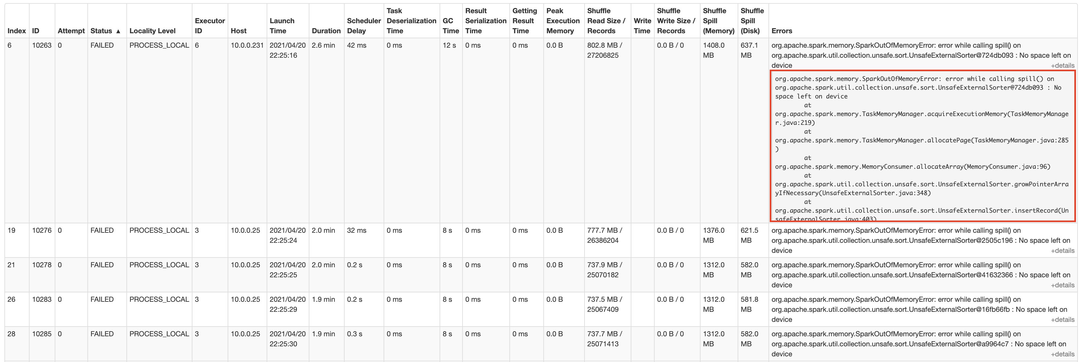
The following screenshot shows the AWS Glue job run details from the Apache Spark web UI:
The job runs for about 1 hour and 25 minutes, then we start observing task failures. Spark ends up stopping the stage and canceling the job when the task retries also fail.
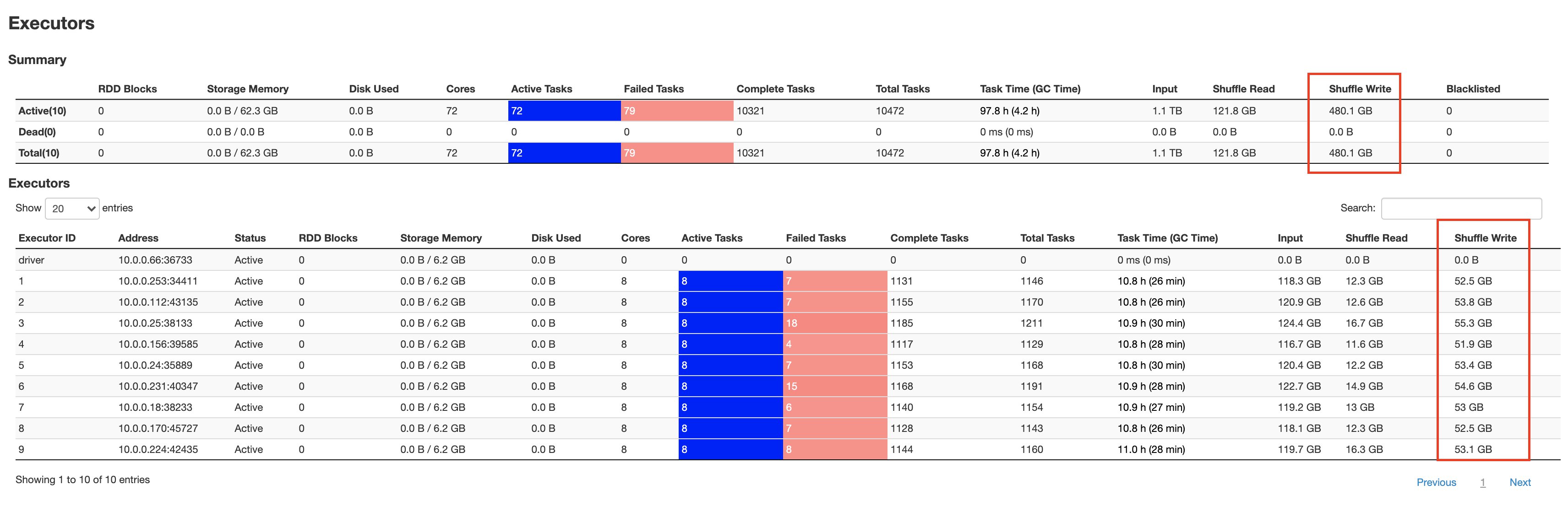
The following screenshots show the aggregated metrics for the failed stage, as well as how much data is spilled to disk by individual executors:
As seen in the Shuffle Write metric from the above Spark UI screenshot, all 10 workers shuffle over 50 GB of data. Further writes aren’t allowed, and tasks start failing with a “No space left on device” error.
The remaining storage is occupied by data that is spilled to disk, as seen in the Shuffle Spill (Disk) metric from the above Spark UI screenshot. This failed job is a classic example of a data-intensive transformation where Spark is both shuffling and spilling to disk when executor memory is filled.
Solution overview
We have various methods for overcoming the disk space error:
Scale out – Increase the number of workers. This incurs an increase in cost. However, scaling out might not always work, especially if your data is heavily skewed on a few keys. Fixing skewness will require considerable modifications to your Spark application logic.
Increase shuffle partitions – Increasing the shuffle partitions can sometimes help overcome space errors. However, this might not always work, and therefore is unreliable.
Disaggregate compute and storage – This approach presents several of the advantages of not only scaling storage for large shuffles, but also adding reliability in the event of node failures because shuffle data is independently stored. Following are few implementations of this disaggregated approach:
Dedicated intermediate storage cluster – In this approach, you use an additional fleet of shuffle services to serve intermediate shuffle. It has several advantages, such as merging shuffle files and sequential I/O, but it introduces an overhead of fleet maintenance from both operations, as well as a cost standpoint. For examples of this approach, see Cosco: An Efficient Facebook-Scale Shuffle Service and Zeus: Uber’s Highly Scalable and Distributed Shuffle as a Service.
Serverless storage – AWS Glue implements a different approach in which you utilize Amazon S3, a cost-effective managed and serverless storage, to store intermediate shuffle data. This design does not depend upon a dedicated daemon, such as shuffle service, to preserve shuffle files. This lets you elastically scale your Spark job without the overhead of running, operating, and maintaining additional storage or compute nodes.
With AWS Glue 2.0, you can now use Amazon S3 to store Spark shuffle and spill data. Amazon S3 is an object storage service that offers industry-leading scalability, data availability, security, and performance. This gives complete elasticity to Spark jobs, thereby allowing you to run your most data intensive workloads reliably.
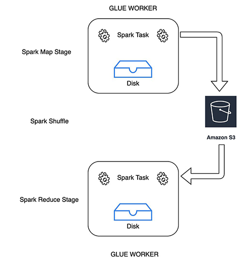
The following diagram illustrates how Spark map tasks write the shuffle and spill files to the given Amazon S3 shuffle bucket. Reducer tasks consider the shuffle blocks as remote blocks and read them from the same shuffle bucket.
Use Amazon S3 to store shuffle and spill data
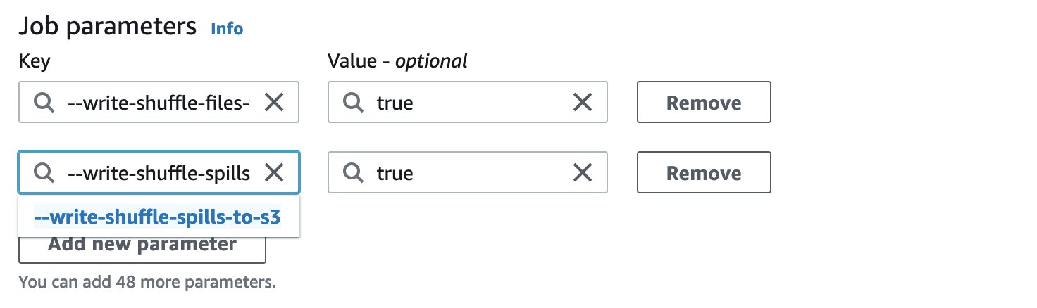
The following job parameters enable and tune Spark to use S3 buckets for storing shuffle and spill data. You can also enable at-rest encryption when writing shuffle data to Amazon S3 by using security configuration settings.
Key
Value
Explanation
–write-shuffle-files-to-s3
TRUE
This is the main flag, which tells Spark to use S3 buckets for writing and reading shuffle data.
–write-shuffle-spills-to-s3
TRUE
This is an optional flag that lets you offload spill files to S3 buckets, which provides additional resiliency to your Spark job. This is only required for large workloads that spill a lot of data to disk. This flag is disabled by default.
This is also optional, and it specifies the S3 bucket where we write the shuffle files. By default, we use —TempDir/shuffle-data.
You can also use the AWS Glue Studio console to enable Amazon S3 based shuffle or spill. You can choose the preceding properties from pre-populated options in the Job parameters section.
Results
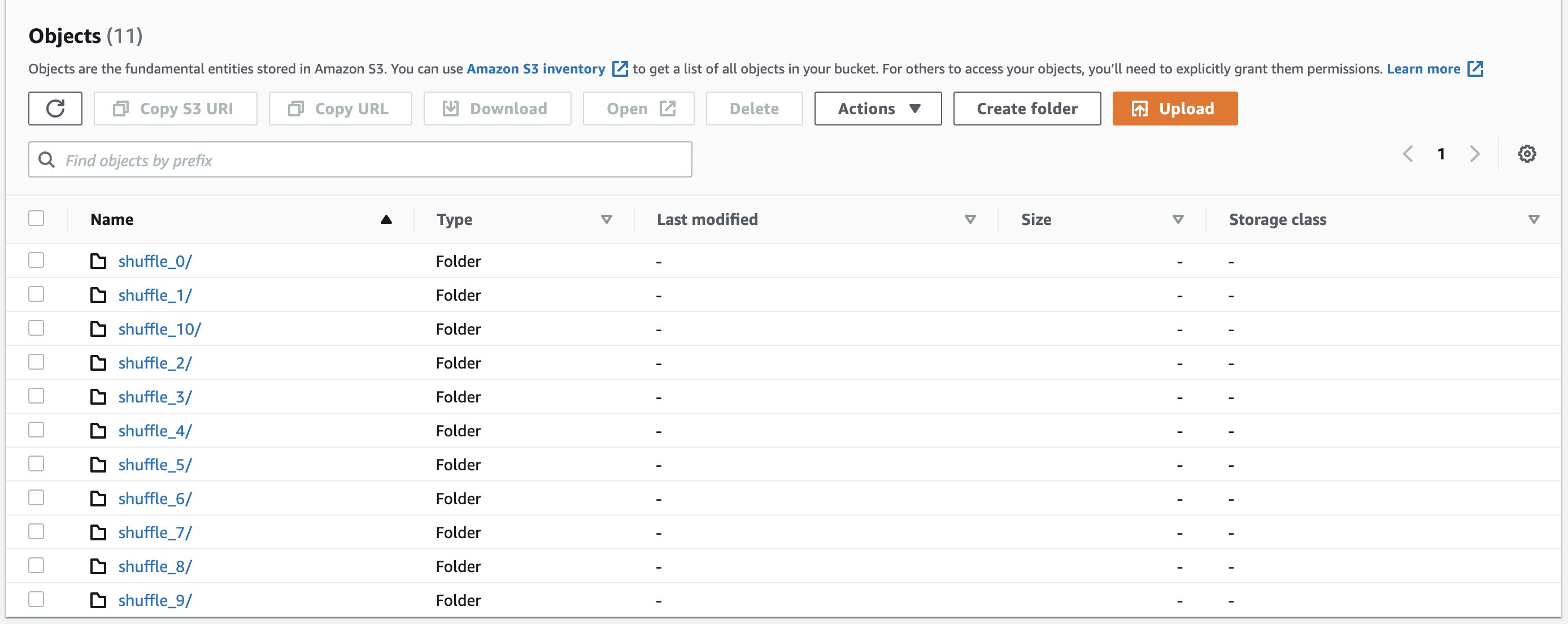
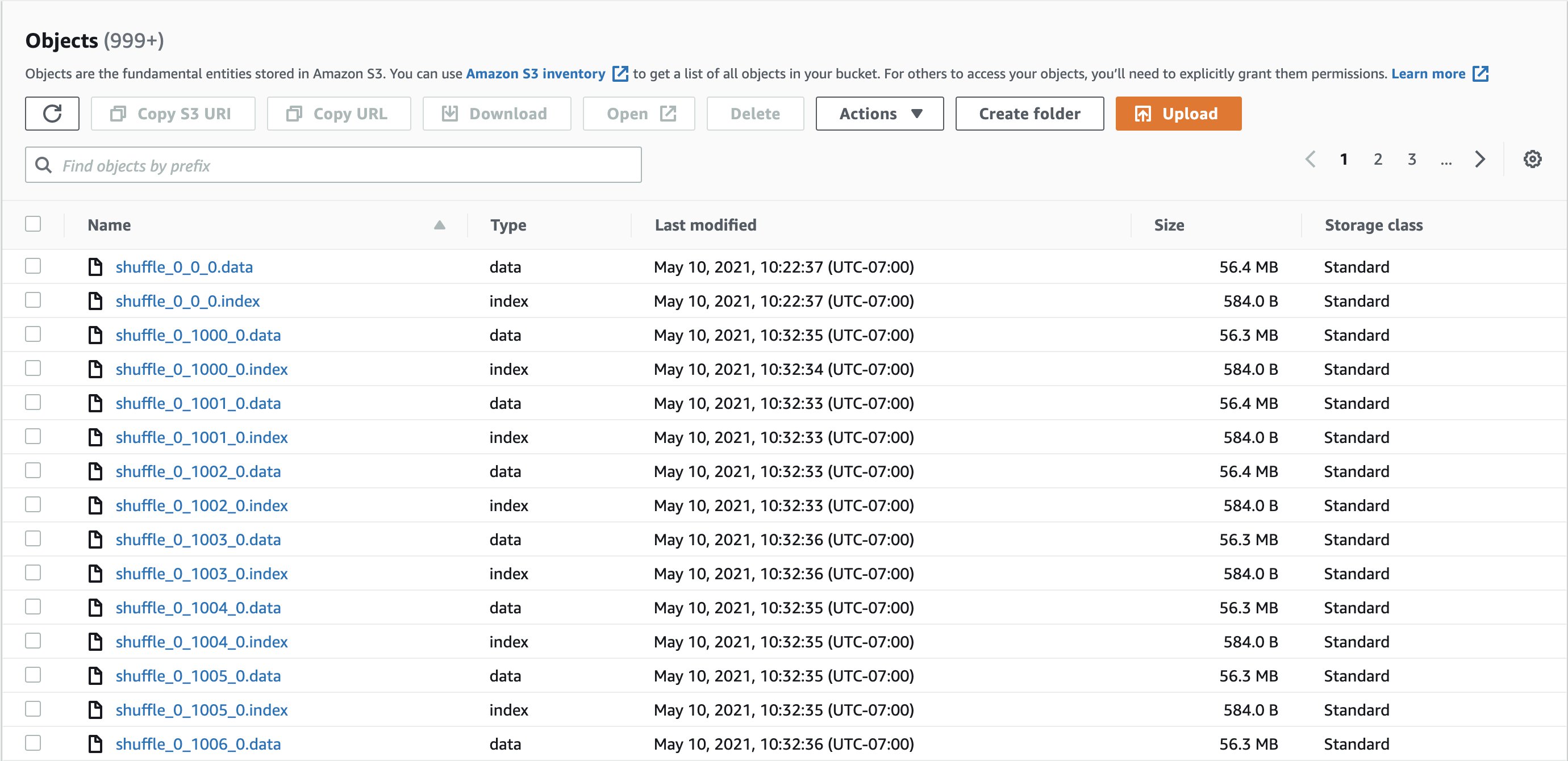
Let’s run the same q80.sql query with Amazon S3 shuffle enabled. We can view the shuffle files stored in the S3 bucket in the following format:
shuffle_<jobid>_<mapperid>_<reducerid>.data/index
Two kinds of files are created:
Data – Stores the shuffle output of the current task
Index – Stores the classification information of the data in the data file by storing partition offsets
The following screenshots shows example shuffle directories and shuffle files:
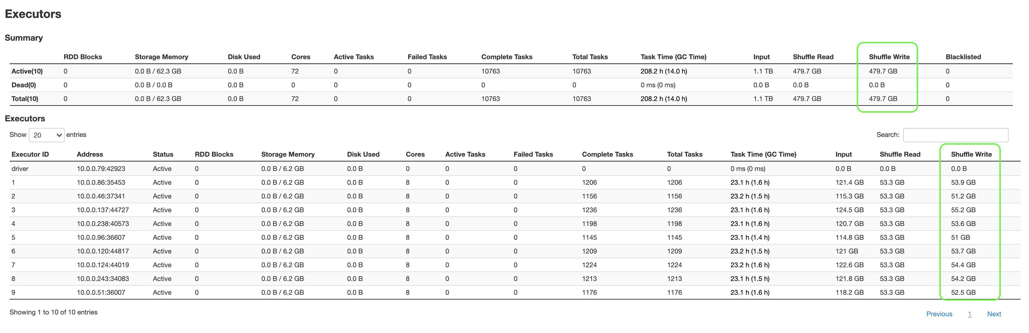
The following screenshot shows the aggregated metrics from the Spark UI:
The following are a few key highlights:
q80.sql, which had failed earlier after 1 hour and 25 minutes, and was able to complete only 13 out of 18 stages, finished successfully in about 2 hours and 53 minutes, completing all 18 stages.
We were able to shuffle 479.7 GB of data without worrying about storage limits.
Additional workers aren’t required to scale storage, which provides substantial cost savings.
Considerations and best practices
Keep in mind the following best practices when considering this solution:
This feature is recommended when you want to ensure the reliable execution of your data intensive workloads that create a large amount of shuffle or spill data. Writing and reading shuffle files from Amazon S3 is marginally slower when compared to local disk for our experiments with TPC-DS queries. S3 shuffle performance would be impacted by the number and size of shuffle files. For example, S3 could be slower for reads as compared to local storage if you have a large number of small shuffle files or partitions in your Spark application.
You can use this feature if your job frequently suffers from No space left on device issues.
You can use this feature if your job frequently suffers fetch failure issues (org.apache.spark.shuffle.MetadataFetchFailedException).
You can use this feature if your data is skewed.
We recommend setting the S3 bucket lifecycle policies on the shuffle bucket (spark.shuffle.glue.s3ShuffleBucket) in order to clean up old shuffle data.
At the time of writing this blog, this feature is currently available on AWS Glue 2.0 and Spark 2.4.3.
Conclusion
This post discussed how we can independently scale storage in AWS Glue without adding additional workers. With this feature, you can expect jobs that are processing terabytes of data to run much more reliably. Happy shuffling!
About the Authors
Anubhav Awasthi is a Big Data Specialist Solutions Architect at AWS. He works with customers to provide architectural guidance for running analytics solutions on Amazon EMR, Amazon Athena, AWS Glue, and AWS Lake Formation.
Rajendra Gujja is a Software Development Engineer on the AWS Glue team. He is passionate about distributed computing and everything and anything to do with the data.
Mohit Saxena is a Software Engineering Manager on the AWS Glue team. His team works on distributed systems for efficiently managing data lakes on AWS and optimizes Apache Spark for performance and reliability.
Marketing teams often rely on data engineers to provide a consumer dataset that they can use to launch marketing campaigns. This can sometimes cause delays in launching campaigns and consume data engineers’ bandwidth. The campaigns are often launched using complex solutions that are either code heavy or using licensed tools. The processes of both extract, transform, and load (ETL) and launching campaigns need engineers who know coding, take time to build, and require maintenance overtime.
You can now simplify this process by integrating AWS services like Amazon PinPoint, AWS Glue DataBrew, and AWS Lambda. We can use DataBrew (a visual data preparation service) to perform ETL, Amazon PinPoint (an outbound and inbound marketing communications service) to launch campaigns, and Lambda functions to achieve end-to-end automation. This solution helps reduce time to production, can be implemented by less-technical folks because it doesn’t require coding, and has no licensing costs involved.
In this post, we walk through the end-to-end workflow and how to implement this solution.
Solution overview
In this solution, the source datasets are pushed to Amazon Simple Storage Service (Amazon S3) using SFTP (batch data) or Amazon API Gateway (streaming data) services. DataBrew jobs perform data transformations and prepare the data for Amazon PinPoint to launch campaigns. We use Lambda to achieve end-to-end automation, which includes an alert system via Amazon Simple Notification Service (Amazon SNS) to alert relevant teams of anomalies or errors.
The workflow includes the following steps:
We can load or push data to Amazon S3 either through AWS Command Line Interface (AWS CLI) commands, AWS access keys, an AWS transfer service (SFTP), or an API Gateway service.
We use DataBrew to perform ETL jobs.
These ETL jobs are either triggered (using Lambda functions) or scheduled.
The processed dataset from DataBrew is imported to Amazon PinPoint as segments using trigger-based Lambda functions.
Marketing teams use Amazon PinPoint to launch campaigns.
We can also perform data profiling using DataBrew.
The following diagram illustrates our solution architecture.
As a bonus step, we can create a simple web portal using AWS Amplify that makes API calls to Amazon PinPoint to launch campaigns in case we want to restrict users from launching campaigns using Amazon PinPoint from the AWS Management Console. This web portal can also provide basic metrics generated by Amazon PinPoint. You can also use it as a product or platform that anyone can use to launch campaigns.
To implement the solution, we complete the following steps:
Create the source datasets using both batch ingestion and Amazon Kinesis streaming services.
Build an automated data ingestion pipeline that transforms the source data and makes it campaign ready.
Build a DataBrew data profile job, after which you can view profile metrics and alert teams in case of any anomalies in the source data.
Launch a campaign using Amazon PinPoint.
Export Amazon PinPoint project events to Amazon S3 using Kinesis Data Firehose.
Create the source datasets
In this step, we create the source datasets from both an SFTP server and Kinesis in Amazon S3.
First, we create an S3 bucket to store the source, processed, and campaign-ready data.
We can ingest data into AWS through many different methods. For this post, we consider methods for batch and streaming ingestion.
For batch ingestion, we create an SFTP-enabled server for source data ingestion. We can configure SFTP servers to store data on either Amazon S3 or Amazon Elastic File System (Amazon EFS). For this post, we configure an SFTP server to store data on Amazon S3.
We use API Gateway and Kinesis for stream ingestion. We can also push data to Kinesis directly, but using API Gateway is preferred because it’s easy to handle cross-account and authentication issues. For instructions on integrating API Gateway and a Kinesis stream, see Tutorial: Create a REST API as an Amazon Kinesis proxy in API Gateway.
Each dataset should be in its own S3 folder: s3://<bucket-name>/src-files/datasource1/, s3://<bucket-name>/src-files/datasource2/, and so on.
Build the automated data ingestion pipeline
In this step, we build the end-to-end automated data ingestion pipeline that transforms the source data and makes it campaign ready.
We use DataBrew for data preparation and data quality, and Lambda and Amazon SNS for automation and alerting. Amazon PinPoint can then use this campaign data to launch campaigns.
Our pipeline performs the following functions:
Run transformations on source datasets.
Merge the datasets to make the data campaign ready.
Perform data quality checks.
Alert relevant teams in case of anomalies in the data quality.
Alert relevant teams in case of DataBrew job failures.
Import the campaign-ready dataset as a segment in Amazon PinPoint.
We can either have one DataBrew project to perform necessary transformations on each dataset and merge all the datasets into one final dataset, or have one DataBrew project for each dataset and another project that merges all the transformed datasets. The advantage of having individual projects for each dataset is that we’re decoupling all data sources, so an issue in one data source doesn’t impact another. We use this latter approach in this post.
DataBrew jobs can be scheduled or trigger based (through a Lambda function). For this post, we configure jobs processing individual data sources to be trigger based, and the final job merging all datasets is scheduled. The advantage of having trigger-based DataBrew jobs is that it only triggers if you have a source file, which helps reduce costs.
We first configure an S3 event that triggers a Lambda function. The function triggers the DataBrew job based on the S3 key value. See the following code (Boto3) for our function:
The processed data appears in s3://<bucket-name>/src-files/process-data/data-source1/.
Next we create the job that merges the processed data files into a final, campaign-ready dataset. We can configure the job to merge only those files that have been dropped in the last 24 hours.
The campaign-ready data is located in s3://<bucket-name>/src-files/campaign-ready/. This dataset is now ready to serve as input to Amazon PinPoint.
Build a DataBrew data profile job
We can use DataBrew to run a data profile job on any of the datasets defined in the previous steps. When you profile your data, DataBrew creates a report called a data profile. This report displays statistics such as the number of rows in the sample and the distribution of unique values in each column. In this post, we use Lambda functions to read the report and detect anomalies and send alerts using Amazon SNS to respective teams for further action.
On the DataBrew console, on the Datasets page, select your dataset.
Choose Run data profile.
For Job name, enter a name for your job.
For Data sample, select either Full dataset or Custom sample (for this post, we sample 20,000 rows).
In the Job output settings section, for S3 location, enter your output bucket.
Optionally, select Enable encryption for job output file to encrypt your data.
Configure optional settings, such as profile configurations; number of nodes, job timeouts, and retries; schedules; and tags.
After you run the job, DataBrew provides you with job metrics. For example, the following screenshot shows the Dataset preview tab.
The following screenshot shows an example of the Data profile overview tab.
This tab also includes a summary of the column details.
The following screenshot shows an example of the Column statistics tab.
Next, we set up alerts using the profile output file.
Configure an S3 event to trigger a Lambda function.
The function reads the output and checks for anomalies in the data. You define the anomalies; for example, when the total missing for a column is greater than 10. The function can then raise an SNS alert if it detects the anomaly.
Launch a campaign using Amazon PinPoint
Before you create segments, create an Amazon PinPoint project. To create segments, we use S3 events to trigger a Lambda function that creates a new base segment whenever the final DataBrew job loads the campaign-ready data. We can either create or update base segments; for this post, we create a new segment. See the following code (Boto3) for the Lambda function:
import boto3
import time
from datetime import datetime

now = datetime.now() # current date and time

date_time = now.strftime("%Y_%m_%d")

segname = segment_name_'+date_time

time.sleep(60)


client = boto3.client('pinpoint')

def lambda_handler(event, context):

response = client.create_import_job(
ApplicationId='xxx-project-id-from-pinpoint',
ImportJobRequest={
'DefineSegment': True,
'Format': 'CSV',
'RoleArn': 'arn:aws:iam::xxx-accountid:role/service-role/xxx_pinpoint_role',
'S3Url': 's3://<xxx-bucketname>/campaign-ready',
'SegmentName': segname
}
)

print(response)
Use this base segment to create dynamic segments and launch a campaign. For more information, see Amazon PinPoint campaigns.
Export Amazon PinPoint project events to Amazon S3 using Kinesis Data Firehose
You can track and push events related to your project, such as sent, delivered, opened messages, and a few others, to either Amazon Kinesis Data Streams or Kinesis Data Firehose, which stream this data to AWS data stores such as Amazon S3. For this post, we use Kinesis Data Firehose. We create our delivery stream prior to enabling event streams on the Amazon PinPoint project.
Select Stream to Amazon Kinesis and select Send events to an Amazon Kinesis Data Firehose delivery stream.
Choose the delivery stream you created.
For IAM role, you can allow DataBrew to automatically create a new role or use an existing role.
Choose Save.
The events are now sent to Amazon S3. You could either create an Athena table or use Amazon Kinesis Data Analytics to analyze events and build a dashboard using QuickSight.
Security best practices
Consider the following best practices in order to mitigate security threats:
Be mindful while creating IAM roles to provide access to only necessary services
If sending emails through Amazon SNS, make sure you send email alerts only to verified or subscribed recipients to minimize the possibility of automated emails being used to target victims’ external email addresses
Use IAM roles rather than user keys
Have logs written to Amazon CloudWatch, and set CloudWatch alarms in case of failures
Take regular backups of DataBrew jobs and Amazon Pinpoint campaigns (if needed)
Restrict network access for inbound and outbound traffic to least privilege
Enable the lifecycle policy to retain only necessary data, and delete unnecessary data
Enable server-side encryption using AWS KMS (SSE-KMS) or Amazon S3 (SSE-S3)
Enable cross-Region replication of data in case you feel backing up the source data is necessary
Clean up
To avoid ongoing charges, clean up the resources you created as part of this post:
S3 bucket
SFTP server
DataBrew resources
PinPoint resources
Firehose delivery stream, if applicable
Athena tables and QuickSight dashboards, if applicable
Conclusion
In this post, we walked through how to implement an automated workflow using DataBrew to perform ETL, Amazon PinPoint to launch campaigns, and Lambda to automate the process. This solution helps reduce time to production, is easy to implement because it doesn’t require coding, and has no licensing costs involved. Try this solution today for your own datasets, and leave any comments or questions in the comments section.
About the Authors
Suraj Shivanandais a Solutions Architect at AWS. He has over a decade of experience in Software Engineering, Data and Analytics, DevOps specifically for data solutions, automating and optimizing cloud based solutions. He’s a trusted technical advisor and helps customers build Well Architected solutions on the AWS platform.
Surbhi Dangi is a Sr Manager, Product Management at AWS. Her work includes building user experiences for Database, Analytics & AI AWS consoles, launching new database and analytics products, working on new feature launches for existing products, and building broadly adopted internal tools for AWS teams. She enjoys traveling to new destinations to discover new cultures, trying new cuisines, and teaches product management 101 to aspiring PMs.
The AWS Architecture Center provides new and notable reference architecture diagrams, vetted architecture solutions, AWS Well-Architected best practices, whitepapers, and more. This blog post features some of our best picks from the new and newly updated content we released in the past month.
The security aspects of additional AWS edge services that you can use to secure your edge environments or expand operations into new, previously unsupported environments
Machine learning (ML) algorithms discover and learn patterns in data and construct mathematical models to enable predictions on future data. ML solutions can revolutionize lives through better diagnosis of diseases, environment protection, products and services transformation, and more.
This newly updated whitepaper provides you with established cloud- and technology-agnostic best practices. Apply these architectural principles when designing your ML workloads or after workloads have entered production as part of continuous improvement.
In this newly published Lens, learn how Well-Architected best practices can help you design, deliver, and maintain streaming media workloads. The Lens defines components, explores common workload scenarios, and outlines design principles that help you apply the Well-Architected Framework. Dive deeper into how each scenario affects the architecture of your workload and evaluate the technology architecture that best meets your needs.
Boost your customer engagement by providing up-to-date product recommendations, personalized product re-rankings, and customized direct marketing. This new Solutions Implementation helps you provide real-time, curated experiences across multiple channels using Amazon Personalize. The implementation automates the entire lifecycle of a personalization workload, presenting the results in an Amazon CloudWatch dashboard.
Alexa, what does a QnABot do? This new Solutions Implementation dives deep on AWS QnABot, a multi-channel, multi-language conversational interface (chatbot) that responds to customer’s questions, answers, and feedback. Learn how to deploy QnABot across channels such as chat, voice, SMS, and Amazon Alexa, implementing the newest ML technologies to enhance the customer experience and build more efficient communications.
Security updates have been issued by Fedora (CuraEngine, curl, firefox, php, and vim), openSUSE (apache2, pcre, salt, transfig, and util-linux), Oracle (.NET 5.0, curl, kernel, libsolv, python3, samba, and webkit2gtk3), and Red Hat (flatpak).
“Once you eliminate the impossible, whatever remains, no matter how improbable, must be the truth.” — Sherlock Holmes
Intro
It’s not every day that you get to debug what may well be a packet of death. It was certainly the first time for me.
What do I mean by “a packet of death”? A software bug where the network stack crashes in reaction to a single received network packet, taking down the whole operating system with it. Like in the well known case of Windows ping of death.
Challenge accepted.
It starts with an oops
Around a year ago we started seeing kernel crashes in the Linux ipv4 stack. Servers were crashing sporadically, but we learned the hard way to never ignore cases like that — when possible we always trace crashes. We also couldn’t tie it to a particular kernel version, which could indicate a regression which hopefully could be tracked down to a single faulty change in the Linux kernel.
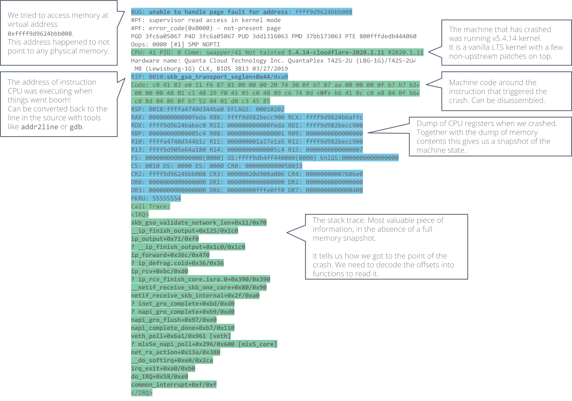
The crashed servers were leaving behind only a crash report, affectionately known as a “kernel oops”. Let’s take a look at it and go over what information we have there.
Parts of the oops, like offsets into functions, need to be decoded in order to be human-readable. Fortunately Linux comes with the decode_stacktrace.sh script that did the work for us.
All we need is to install a kernel debug and source packages before running the script. We will use the latest version of the script as it has been significantly improved since Linux v5.4 came out.
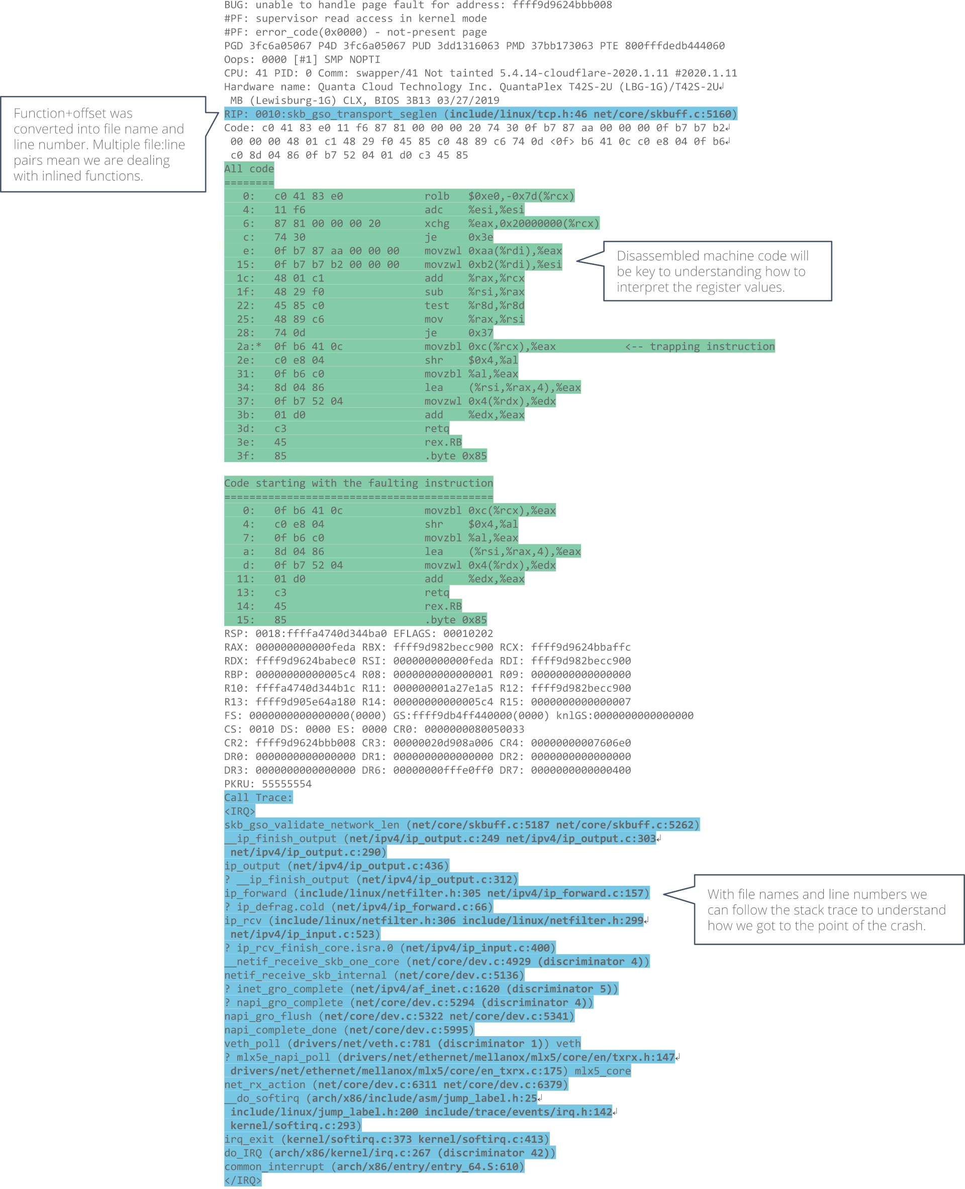
When decoded, the oops report is even longer than before! But that is a good thing. There is new information there that can help us.
What has happened?
With this much input we can start sketching a picture of what could have happened. First thing to check is where exactly did we crash?
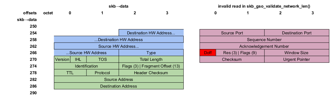
The report points at line 5160 in the skb_gso_transport_seglen() function. If we take a look at the source code, we can get a rough idea of what happens there. We are processing a Generic Segmentation Offload (GSO) packet carrying an encapsulated TCP packet. What is a GSO packet? In this context it’s a batch of consecutive TCP segments, travelling through the network stack together to amortize the processing cost. We will look more at the GSO later.
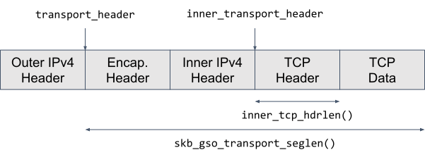
The exact line where we crashed belongs to an if-branch that handles tunnel traffic. It calculates the length of the TCP header of the inner packet, that is the encapsulated one. We do that to compute the length of the outer L4 segment, which accounts for the inner packet length:
To understand how the length of the inner TCP header is computed we have to peel off a few layers of inlined function calls:
Now it is clear that inner_tcp_hdrlen(skb) simply reads the Data Offset field (doff) inside the inner TCP header. Because Data Offset carries the number of 32-bit words in the TCP header, we multiply it by 4 to get the TCP header length in bytes.
From the memory access point of view, to read the Data Offset value we need to:
load skb->head value from address skb + offsetof(struct sk_buff, head)
load skb->inner_transport_header value from address skb + offsetof(struct sk_buff, inner_transport_header),
load the TCP Data Offset from skb->head + skb->inner_transport_header + offsetof(struct tcphdr, doff)
Potentially, any of these loads could trigger a page fault. But it’s unlikely that skb contains an invalid address since we accessed the skb->encapsulation field without crashing just a few lines earlier. Our main suspect is the last load.
The invalid memory address we attempt to load from should be in one of the CPU registers at the time of the exception. And we have the CPU register snapshot in the oops report. Which register holds the address? That has been decided by the compiler. We will need to take a look at the instruction stream to discover that.
Remember the disassembly in the decoded kernel oops? Now is the time to go back to it. Hint, it’s in AT&T syntax. But to give everyone a fair chance to follow along, here’s the same disassembly but in Intel syntax. (Alright, alright. You caught me. I just can’t read the AT&T syntax.)
When the trapped page fault happened, we tried to load from address %rcx + 0xc, or 12 bytes from whatever memory location %rcx held. Which is hardly a coincidence since the Data Offset field is 12 bytes into the TCP header.
This means that %rcx holds the computed skb->head + skb->inner_transport_header address. Let’s take a look at it:
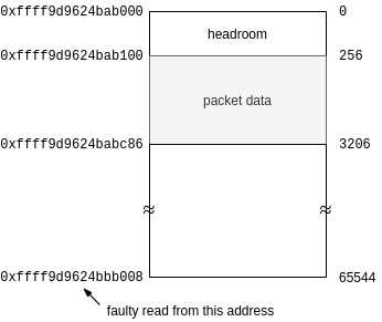
The RCX value doesn’t look particularly suspicious. We can say that:
it’s in a kernel virtual address space because it is greater than 0xffff000000000000 – expected, and
it is very close to the 4 KiB page boundary (0xffff9d9624bbb000 – 4),
… and not much more.
We must go back further in the instruction stream. Where did the value in %rcx come from? What I like to do is try to correlate the machine code leading up to the crash with pseudo source code:
How did I decode that assembly snippet? We know that the skb address was passed to our function in the %rdi register because the System V AMD64 ABI calling convention dictates that. If the %rdi register hasn’t been clobbered by any function calls, or reused because the compiler decided so, then maybe, just maybe, it still holds the skb address.
If 0xaa and 0xb2 are offsets into an sk_buff structure, then pahole tool can tell us which fields they correspond to:
It would be great to find out the value of the inner_transport_header and transport_header offsets. But the registers that were holding them, %rax and %rsi, respectively, were reused after the offset values were loaded.
However, we can still examine the difference between inner_transport_header and transport_header that both %rax and %rsi hold. Let’s take a look.
The suspicious offset
Here are the register values from the oops as a reminder:
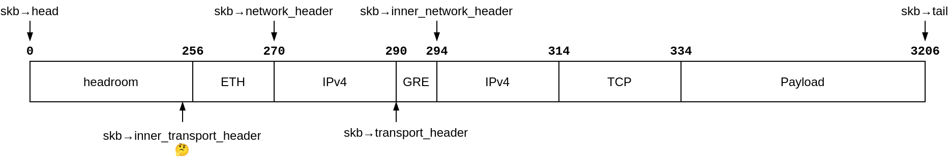
That is clearly suspicious. We expect that skb->transport_header < skb->inner_transport_header, so either
skb->inner_transport_header > 0xfeda, which would mean that between outer and inner L4 packets there is 65k+ bytes worth of headers – unlikely, or
0xfeda is a garbage value, perhaps an effect of an underflow if skb->inner_transport_header < skb->transport_header.
Let’s entertain the theory that an underflow has occurred.
Any other scenario, be it an out-of-bounds write or a use-after-free that corrupted the memory, is a scary prospect where we don’t stand much chance of debugging it without help from tools like KASAN report.
But if we assume for a moment that it’s an underflow, then the task is simple 😉. We “just” need to audit all places where skb->inner_transport_header or skb->transport_header offsets could have been updated while the skb buffer travelled through the network stack.
That raises the question — what path did the packet take through the network stack before it brought the machine down?
Packet path
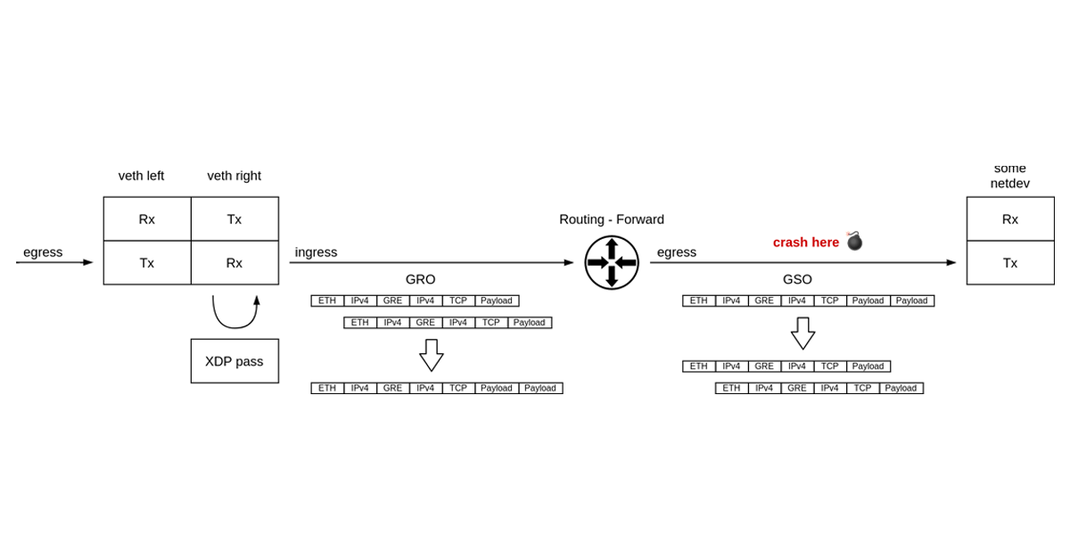
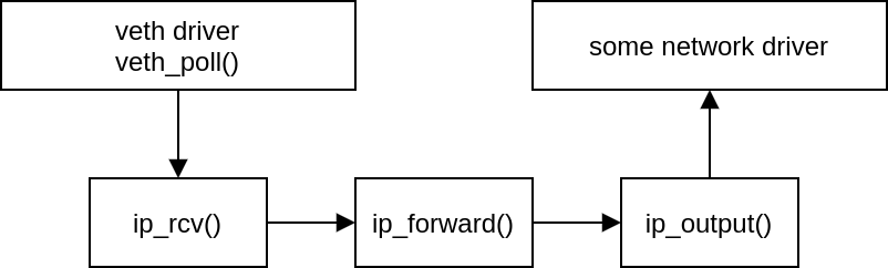
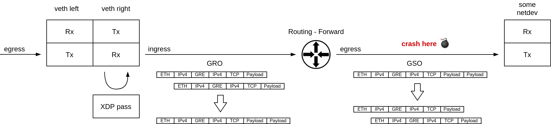
It is time to take a look at the call trace in the oops report. If we walk through it, it is apparent that a veth device received a packet. The packet then got routed and forwarded to some other network device. The kernel crashed before the egress device transmitted the packet out.
What immediately draws our attention is the veth_poll() function in the call trace. Polling inside a virtual device that acts as a simple pipe joining two network namespaces together? Puzzling!
The regular operation mode of a veth device is that transmission of a packet from one side of a veth-pair results in immediate, in-line, on the same CPU, reception of the packet by the other side of the pair. There shouldn’t be any polling, context switches or such.
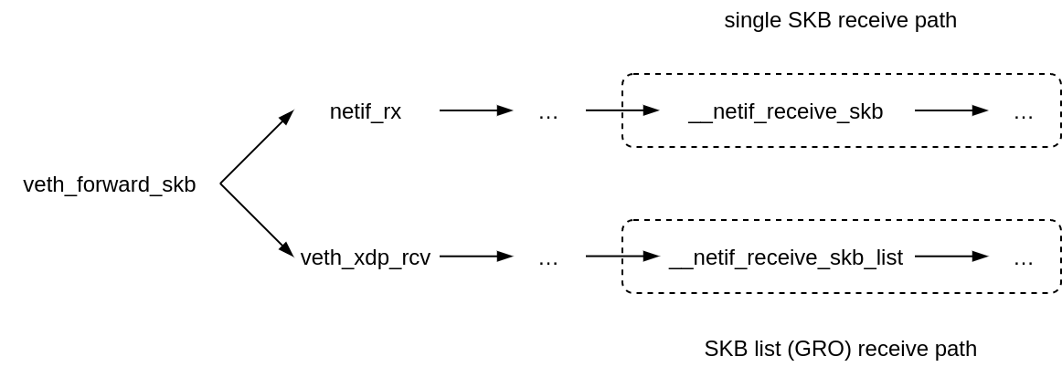
The NAPI receive path in the veth driver is taken only when there is an XDP program attached. The fork occurs in veth_forward_skb, where the TX path ends and a RX path on the other side begins.
This is an important observation because only on the NAPI/XDP path in the veth driver, received packets might get aggregated by the Generic Receive Offload.
Super-packets
Early on we’ve noted that the crash happens when processing a GSO packet. I’ve promised we will get back to it and now is the time.
Generic Segmentation Offload (GSO) is all about delaying the L4 segmentation process until the very last moment. So called super-packets, that exceed the egress route MTU in size, travel all the way through the network stack, only to be cut into MTU-sized segments just before handing the data over to the network driver for transmission. This way we process just one big packet on the transmit path, instead of a few smaller ones and save on CPU cycles in all the IP-level stack functions like routing, nftables, traffic control
Where do these super-packets come from? They can be a result of large write to a socket, or as is our case, they can be received from one network and forwarded to another network.
The latter case, that is forwarding a super-packet, happens when Generic Receive Offload (GRO) kicks in during receive. GRO is the opposite process of GSO. Smaller, MTU-sized packets get merged to form a super-packet early on the receive path. The goal is the same — process less by pushing just one packet through the network stack layers.
Not just any packets can be fused together by GRO. Loosely speaking, any two packets to be merged must form a logical sequence in the network flow, and carry the same metadata in protocol headers. It is critical that no information is lost in the aggregation process. Otherwise, GSO won’t be able to reconstruct the segment stream when serializing packets in the network card transmission code.
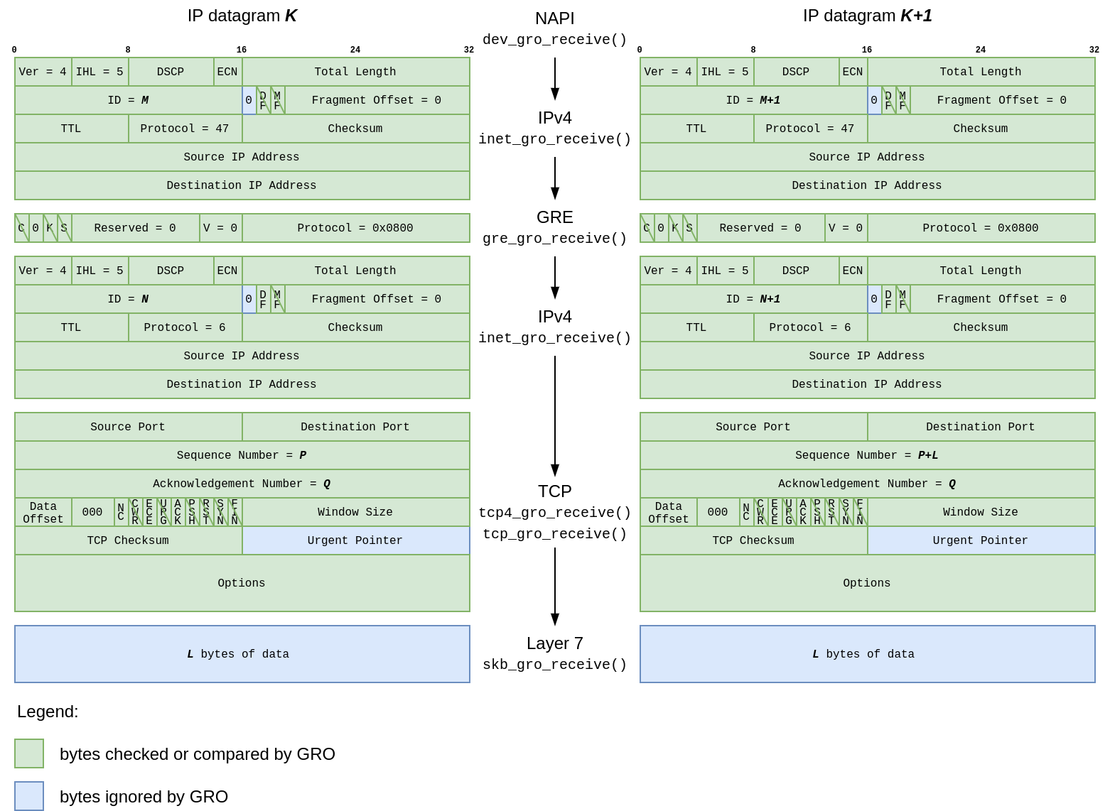
To this end, each network protocol that supports GRO provides a callback which signals whether the above conditions hold true. GRO implementation (dev_gro_receive()) then walks through the packet headers, the outer as well as the inner ones, and delegates the pre-merge check to the right protocol callback. If all stars align, the packets get spliced at the end of the callback chain (skb_gro_receive()).
I will be frank. The code that performs GRO is pretty complex, and I spent a significant amount of time staring into it. Hat tip to its authors. However, for our little investigation it will be enough to understand that a TCP stream encapsulated with GRE1 would trigger callback chain like so:
Armed with basic GRO/GSO understanding we are ready to take a shot at reproducing the crash.
The reproducer
Let’s recap what we know:
a super-packet was received from a veth device,
the veth device had an XDP program attached,
the packet was forwarded to another device,
the egress device was transmitting a GSO super-packet,
the packet was encapsulated,
the super-packet must have been produced by GRO on ingress.
This paints a pretty clear picture on what the setup should look like:
We will be sending traffic from 10.1.1.1 to 10.2.2.2. Our traffic pattern will be a TCP stream consisting of two consecutive segments so that GRO can merge something. A Scapy script will be great for that. Let’s call it send-a-pair.py and give it a run:
$ { sleep 5; sudo ip netns exec A ./send-a-pair.py; } &
[1] 1603
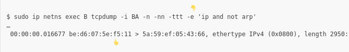
$ sudo ip netns exec B tcpdump -i BA -n -nn -ttt 'ip and not arp'
…
00:00:00.020506 IP 10.1.1.1 > 10.2.2.2: GREv0, length 1480: IP 192.168.1.1.12345 > 192.168.2.2.443: Flags [.], seq 0:1436, ack 1, win 8192, length 1436
00:00:00.000082 IP 10.1.1.1 > 10.2.2.2: GREv0, length 1480: IP 192.168.1.1.12345 > 192.168.2.2.443: Flags [.], seq 1436:2872, ack 1, win 8192, length 1436
Where is our super-packet? Look at the packet sizes, the GRO didn’t merge anything.
Turns out NAPI is just too fast at fetching the packets from the Rx ring. We need a little buffering on transmit to increase our chances of GRO batching:
# Help GRO
ip netns exec A tc qdisc add dev AB root netem delay 200us slot 5ms 10ms packets 2 bytes 64k
…but we are not crashing. We will need to dig deeper.
We know what packet metadata skb_gso_transport_seglen() looks at — the header offsets, then encapsulation flag, and GSO info. Let’s dump all of it:
$ sudo bpftrace ./why-no-crash.bt -c '/usr/bin/ip netns exec A ./send-a-pair.py'
Attaching 2 probes...
DEV  LEN  NH  TH  ENC INH ITH GSO SIZE SEGS TYPE FUNC
sink 2936 270 290 1   294 254  |  1436 2    0x41 skb_gso_transport_seglen
Since the skb->encapsulation flag (ENC) is set, both outer and inner header offsets should be valid. Are they?
The outer network / L3 header (NH) looks sane. When XDP is enabled, it reserves 256 bytes of headroom before the headers. 14 byte long Ethernet header follows the headroom. The IPv4 header should then start at 270 bytes into the packet buffer.
The outer transport / L4 header offset is as expected as well. The IPv4 header takes 20 bytes, and the GRE header follows it.
The inner network header (INH) begins at the offset of 294 bytes. This makes sense because the GRE header in its most basic form is 4 bytes long.
The surprise comes last. The inner transport header offset points somewhere near the end of headroom which XDP reserves. Instead, it should start at 314, following the inner IPv4 header.
Is this the smoking gun we were looking for?
The bug
skb_gso_transport_seglen() calculates the length of the outer L4 segment when given a GSO packet. If the inner_transport_header offset is off, then the result of the calculation might be off as well. Worth checking.
We know that our segments are 1500 bytes long. That makes the L4 part 1480 bytes long. What does skb_gso_transport_seglen() say though?
Seems that we don’t agree. But if skb_gso_transport_seglen() is getting garbage on input we can’t really blame it.
If inner_transport_header is not correct, that TCP Data Offset read that we know happens inside the function cannot end well.
If we map it out, it looks like we are loading part of the source MAC address (upper 4 bits of the 5th byte, to be precise) and interpreting it as TCP Data Offset.
Are we? There is an easy way to check.
If we ask nicely, tcpdump will tell us what the MAC addresses are:
Plugging that into the calculations that skb_gso_transport_seglen() …
Does this mean that I can control the return value by setting source MAC address?!
                                               👇
$ sudo ip -n A link set AB address be:d6:07:5e:05:11 # Change the MAC address
$ sudo bpftrace -e 'kretprobe:skb_gso_transport_seglen { print(retval); }' -c …
Attaching 1 probe...
1400
Yes! 1436 + (-36) + (0 * 4) = 1400. This is it.
However, how does all this tie it to the original crash? The badly calculated L4 segment length will make GSO emit shorter segments on egress. But that’s all.
Remember the suspicious offset from the crash report?
Solving it for skb->head yields 0xffff9d9624bbb008 - 0xfffc - 12 = 0xffff9d9624bab000.
And this makes sense. The skb->head buffer is page-aligned, meaning it’s a multiple of 4 KiB on x86-64 platforms — the 12 least significant bits the address are 0.
However, the address we were trying to read was (0xfffc+12)/4096 ~= 16 pages (or 64 KiB) past the skb->head page boundary (0xffff9d9624babfff).
Who knows if there was memory mapped to this address?! Looks like from time to time there wasn’t anything mapped there and the kernel page fault handling code went “oops!”.
The fix
It is finally time to understand who sets the header offsets in a super-packet.
Once GRO is done merging segments, it flushes the super-packet down the pipe by kicking off a chain of gro_complete callbacks:
These callbacks are responsible for updating the header offsets and populating the GSO-related fields in skb_shared_info struct. Later on the transmit side will consume this data.
Let’s see how the packet metadata changes as it travels through the gro_complete callbacks2 by adding a few more tracepoint to our bpftrace script:
As the packet travels through the gro_complete callbacks, the inner network header (INH) offset gets updated after we have processed the inner IPv4 header.
However, the same thing did not happen to the inner transport header (ITH) that is causing trouble. We need to fix that.
--- a/net/ipv4/tcp_offload.c
+++ b/net/ipv4/tcp_offload.c
@@ -298,6 +298,9 @@ int tcp_gro_complete(struct sk_buff *skb)
        if (th->cwr)
                skb_shinfo(skb)->gso_type |= SKB_GSO_TCP_ECN;

+       if (skb->encapsulation)
+               skb->inner_transport_header = skb->transport_header;
+
        return 0;
 }
 EXPORT_SYMBOL(tcp_gro_complete);
With the patch in place, the header offsets are finally all sane and skb_gso_transport_seglen() return value is as expected:
Don’t worry, though. The fix is already likely in your kernel long time ago. Patch d51c5907e980 (“net, gro: Set inner transport header offset in tcp/udp GRO hook”) has been merged into Linux v5.14, and backported to v5.10.58 and v5.4.140 LTS kernels. The Linux kernel community has got you covered. But please, keep on updating your production kernels.
Outro
What a journey! We have learned a ton and fixed a real bug in the Linux kernel. In the end it was not a Packet of Death. Maybe next time we can find one 😉
Enjoyed the read? Why not join Cloudflare and help us fix the remaining bugs in the Linux kernel? We are hiring in Lisbon, London, and Austin.
And if you would like to see more kernel blog posts, please let us know!
… 1Why GRE and not some other type of encapsulation? If you follow our blog closely, you might already know that Cloudflare Magic Transit uses veth pairs to route traffic into and out of network namespaces. It also happens to use GRE encapsulation. If you are curious why we chose network namespaces linked with veth pairs, be sure to watch the How we built Magic Transit talk. 2Just turn off GRO on all other network devices in use to get a clean output (sudo ethtool -K enp0s5 gro off).
Have you ever tried to figure out why a vulnerability or policy scan isn’t showing you the results you expect, even though you’ve provided credentials? If so, you’ll be pleased to hear that the November 3rd release of Nexpose and InsightVM (version 6.6.111) will introduce a new check category designed to help troubleshoot issues with credentialed scanning: Scan Diagnostics.
No more combing through scan logs to get answers! These checks will be disabled by default, but you can configure them to run by adjusting your scan templates. When enabled, Scan Diagnostics checks will report a “vulnerable” result against assets when the Scan Engine is supplied with credentials but unable to gather local information.
The challenge of finding the right fix
For complete and accurate coverage, the InsightVM Scan Engine requires local access to systems being scanned. Most Microsoft checks are based on values found in the Windows Registry. Checks for Linux distributions typically require access to the package manager, which is important for vulnerability correlation (cutting down on noise due to backported fixes).
This means that for many types of scans, you need to tell the engine how it should authenticate by configuring credentials. When things go smoothly, the engine will collect all the data it needs for vulnerability or policy assessments. But when results aren’t as expected, it can be challenging to understand what went wrong.
The way the Security Console currently indicates authentication status results is rather coarse-grained. Credential Success means it’s all good, but a Credential Failure (or the puzzling “Partial Credential Success”) can often leave a VM analyst scratching their head about how to fix things.
Bringing greater visibility to your scanning environment
Our new Scan Diagnostics checks provide more detailed visibility into where things fell apart. Because the results are written as vulnerability checks, you’ll be able to use a lot of familiar product functionality to work with them. They can be enabled or disabled via scan templates, and you can report on them like any other category. We’ll also be providing solution information to make it easier to resolve issues, and you can look at the proof the scanner provides to get additional context.
Another advantage of using check results for Scan Diagnostics is that they are built atop the expert system at the core of the scanner. This helps Scan Diagnostics target the most precise cause of an error and provide guidance accordingly. No more going through a laundry list of checkboxes to make sure your sites and assets are configured correctly.
Here is the initial set of Scan Diagnostics we’ll be releasing:
Error when connecting to DCOM Ports (required for WMI)
rapid7-diagnostics-wmi-permission-error
Permission error when connecting to the WMI Service
rapid7-diagnostics-wmi-read-access-errors
Access errors encountered in attempts to read over WMI
rapid7-diagnostics-wmi-unknown-error
Unknown error occurred trying to connect to the WMI Service
rapid7-diagnostics-winrm-authentication-error
Authentication error when connecting to the WMI Service
rapid7-diagnostics-winrm-listener-error
The WinRM listener on the target appears to be blocking the scan engine from connecting
rapid7-diagnostics-winrm-unknown-error
Unknown error occurred trying to connect to the WinRM Service
rapid7-diagnostics-winrm-unencrypted
The WinRM service is operating over an unencrypted protocol, potentially leaking valuable data
Note that these “vulnerabilities” carry the lowest possible severity and will not increase your risk score. However, they may increase overall vulnerability counts, so we’re leaving them turned off by default for now. If you do scan with them, you can adjust the scope of generated reports to exclude these results if you don’t want them to get passed through to remediation teams.
The existing status shown in the Authentication column of Scan Results and Node pages will remain the same for the time being, so that it is available regardless of whether this new Scan Diagnostics check type is enabled and won’t adjust anything on the corresponding dashboard card.
We’d love to hear any feedback on this new feature! Please reach out to your Customer Success Manager to let them know how it’s working out in your scans.
NEVER MISS A BLOG
Get the latest stories, expertise, and news about security today.
To provide the best experiences, we use technologies like cookies to store and/or access device information. Consenting to these technologies will allow us to process data such as browsing behavior or unique IDs on this site. Not consenting or withdrawing consent, may adversely affect certain features and functions.
Functional
Always active
The technical storage or access is strictly necessary for the legitimate purpose of enabling the use of a specific service explicitly requested by the subscriber or user, or for the sole purpose of carrying out the transmission of a communication over an electronic communications network.
Preferences
The technical storage or access is necessary for the legitimate purpose of storing preferences that are not requested by the subscriber or user.
Statistics
The technical storage or access that is used exclusively for statistical purposes.The technical storage or access that is used exclusively for anonymous statistical purposes. Without a subpoena, voluntary compliance on the part of your Internet Service Provider, or additional records from a third party, information stored or retrieved for this purpose alone cannot usually be used to identify you.
Marketing
The technical storage or access is required to create user profiles to send advertising, or to track the user on a website or across several websites for similar marketing purposes.
![[Security Nation] Pete Cooper and Irene Pontisso of the UK Cabinet Office on Their Cybersecurity Culture Competition](https://blog.rapid7.com/content/images/2021/11/image1.jpg)
![[Security Nation] Pete Cooper and Irene Pontisso of the UK Cabinet Office on Their Cybersecurity Culture Competition](https://blog.rapid7.com/content/images/2021/11/irene_pontisso.jpg)