Where and Why Object Storage Excels Throughout the AI Model Lifecycle

Post Syndicated from David Johnson original https://www.backblaze.com/blog/where-and-why-object-storage-excels-throughout-the-ai-model-lifecycle/

A decorative image showing a multi-paned screen backed up by a cloud.

No single technology has changed the way we use data quite like AI. From massive training sets to constant streams of checkpoint and inference data, AI applications are data intensive, to say the least.
Thankfully, there’s an answer. Object storage—with its scalability, flexibility, and cost-effectiveness—is uniquely suited to AI at every stage of the model lifecycle.

In this blog post, we’ll take a quick look at what object storage is, why it’s a perfect fit for AI workloads, and how Backblaze B2 Cloud Storage offers unique advantages for AI teams looking to innovate quickly, easily, and cost-effectively.

What is object storage?

Think of object storage as a giant, organized bucket for all your files. Instead of stuffing things into folders or breaking them into blocks, you just drop each file (an “object”), with a unique tag and some helpful notes (metadata), into your storage solution.

Unlike traditional file or block storage, object storage uses a flat address space. Each object is assigned a unique identifier and can be tagged with rich metadata, making it easy to search, retrieve, and manage at scale.

Because of this unique architecture, object storage is ideal for handling unstructured data—such as images, video, audio, text, and sensor data—which is the meat and potatoes of most modern AI workflows. Also, being cloud-based, object storage is inherently designed for massive scalability and accessibility over the internet (often via S3 API).

Ebook: “Why Object Storage Is Ideal for AI Workflows”

Want to take a deeper dive into the world of object storage? Check out our latest ebook, “Why Object Storage is Ideal for AI Workloads,” and discover the advantages this architecture has to offer across the model lifecycle.

Get the Ebook

Understanding AI’s data storage needs at each stage of the model lifecycle

Before diving into the benefits of object storage, let’s first define and outline the AI model lifecycle. While some may slice and dice it a little differently, generally speaking, we can break the AI model lifecycle down into the following stages:

  • Data ingestion and collection: Massive, often petabyte-scale datasets are gathered from a diversity of sources.
  • Data preparation and storage: Raw data is cleaned, labeled, transformed, and stored for future retrieval and processing.
  • Model training: Data is fed into AI training algorithms, typically deployed across many nodes in a GPU cluster—usually requiring high throughput, parallel access, and lengthy processing times.
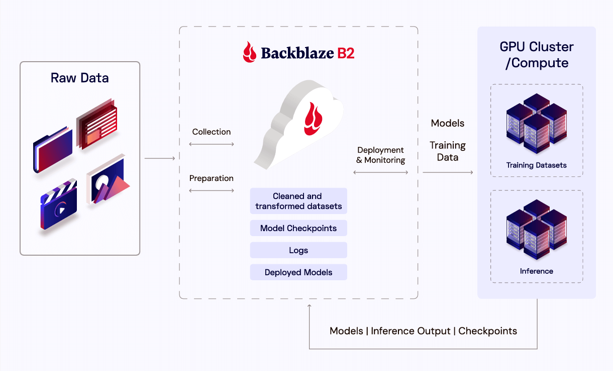
  • Deployment and inference: Trained models are deployed into live applications where they take in new data and make inferences based on that data.
  • Monitoring and archiving: Continuous monitoring generates substantial amounts of log data and performance metrics that must be versioned, stored, and archived for compliance or retraining purposes.

As you can see, each stage of the model lifecycle presents its own unique set of data demands—with each one requiring plenty of planning, work, and preparation. And at every one of these stages, matters of scale, speed, accessibility, and cost are mission-critical to a project’s success. 

Where object storage excels: Scalability for data ingestion and collection

Object storage offers virtually unlimited scalability for large, and ever-expanding datasets, making it an ideal solution for the earliest stages of AI development. With no need to create volumes or file systems, organizations can quickly start uploading data to object storage. In addition to this seamless scalability, object storage also shines in its ability to support a diverse range of structured and unstructured data types without the need for rigid hierarchies. In this way, AI teams can ingest all sorts of data to support whatever their unique application needs; and do it quickly and efficiently.

Flexible data preparation and storage

Cloud-based object storage systems are excellent for maintaining easily-accessible, version-controlled datasets that allow for lightning fast iteration and collaboration. Capabilities like version recovery (which allows teams to easily revert datasets to previous states with simple API calls) and concurrent access (which gives multiple team members the ability to work on the same datasets simultaneously without conflicts) are also key to the data preparation and storage phase of AI development.

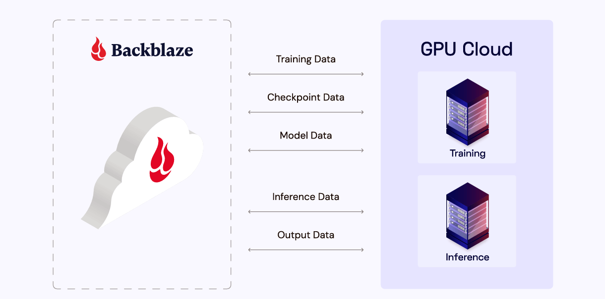
Reliable, high-performance data storage for model training

For the model training stage of the AI lifecycle, object storage supports parallel access and high throughput, both of which are absolutely essential for GPU-intensive training workloads. Reliable shuttling of large datasets to GPU clusters, wherever they may be, is key for keeping things efficient. Meanwhile, streamlined storage of model checkpoints from those clusters gives teams peace of mind in knowing that a mid-training failure state will not place them all the way back at square one.

Plus, lifecycle management features allow completed or outdated training datasets to be automatically archived—reducing clutter and optimizing storage costs, all while keeping active training data easily accessible.

Efficient versioning for deployment and inference

AI models are always a work in progress. Once deployed and operational, they have to be routinely evaluated and tuned. To that end, object storage makes it easy to store and retrieve a range of valuable information, including model checkpoints, test results, and inference data.

Built-in versioning and object immutability features support reproducibility and audit trails, so you can always trace which data and models produced which results. Together, these capabilities make for robust and effective lifecycle management, significantly boosting reliability and compliance.

Cost-effectiveness and durability for monitoring and archiving

When in the field, continuous monitoring of AI models generates a whole lot of log data and performance metrics. Object storage automates the management of these resources through customizable lifecycle rules, automatically deleting or archiving out-of-date inference logs based on predefined timelines (e.g., after 30–180 days).

This significantly reduces the need for manual oversight, conserves engineering resources, and ensures that relevant performance data remains accessible for compliance and regulatory auditing.

Meanwhile, with the right vendor, object storage solutions can offer competitive pricing models—sometimes including the separation of compute from storage—to ensure cost-effectiveness throughout the late stages of the AI lifecycle. Finally, high durability (of 11 nines or more) and redundancies protect models and datasets which become increasingly valuable over time.

Backblaze B2: Cost-effective, high-performance object storage for your AI workloads

Backblaze B2 Cloud Storage takes all the inherent advantages of cloud-based object storage for AI workloads and amplifies them—through competitive, transparent pricing; reliable, high performance; and seamless integration and support to ensure your project is not only efficient and affordable, but most importantly, successful

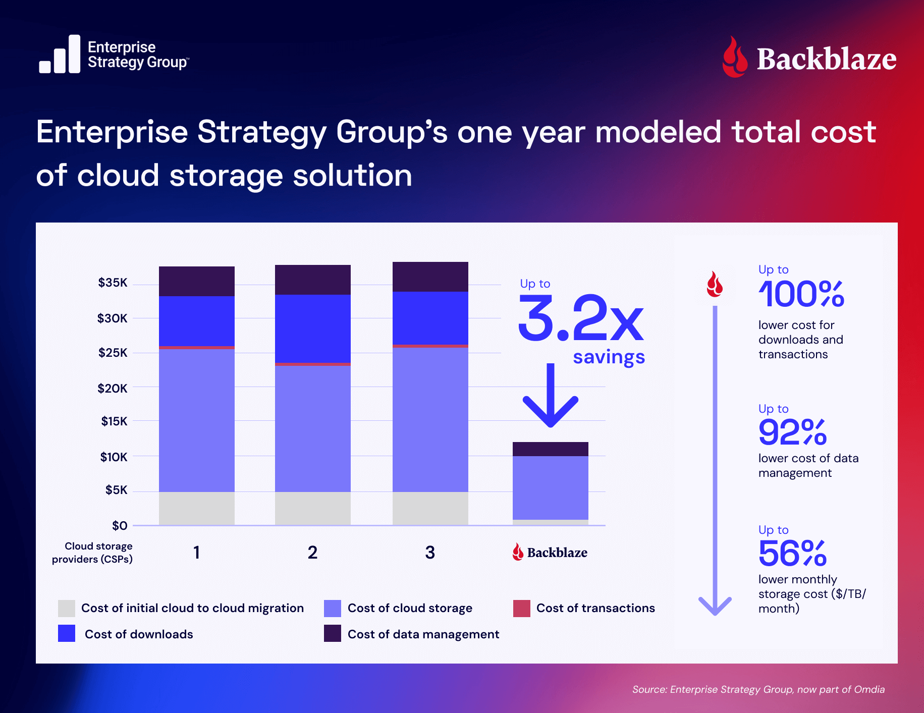
  • Competitive, transparent pricing: One-fifth of the cost of most hyperscalers’ solutions, with no hidden costs and three times your total storage volume in free egress included. Plus, fully-transparent, predictable pricing models ensure your organization is fully aware and prepared for the costs associated with your applications. 
  • High performance and reliability: Upload speeds up to 30% faster than AWS S3 for many workloads, plus a 99.9% uptime SLA with 11 nines of durability, ensure always-hot, instantly accessible data for demanding AI workloads. 
  • Seamless adoption and integration, accompanied by expert support: With features like Universal Data Migration and no hidden delete fees, B2 Cloud Storage uniquely streamlines cost-effective data management for AI. Backblaze B2 also boasts S3 API compatibility for true plug-and-play functionality with leading AI and machine learning ops (MLOps) tools and technologies.

Plus, our truly agnostic solution allows organizations to freely and easily connect to any compute or GPU environment (or environments), free of vendor lock-in and fees. And in case you want some support along the way, our team of dedicated solution engineers are available to tailor and fine-tune your architecture and operations to best suit whatever the unique needs of your AI project may be. 

Optimize your AI lifecycle with cloud object storage from Backblaze B2

Data is one of the most important, and most challenging, aspects of AI development. And with their unprecedented data demands, traditional block and file storage systems frequently come up short in supporting modern AI applications. At the same time, legacy cloud storage solutions come with enormous burdens of cost, inflexibility, and the ever-looming threat of lock-in.

Cloud-based object storage offers the perfect solution to all these challenges—with the right mixture of performance, efficiency, and cost-effectiveness that AI projects need.It’s so-well-suited, in fact, that we’ve written an entire white paper on the subject! So, if you’re interested in taking a deeper dive into the topic, check out our ebook, Why Object Storage is Ideal for AI Workloads, today.

The post Where and Why Object Storage Excels Throughout the AI Model Lifecycle appeared first on Backblaze Blog | Cloud Storage & Cloud Backup

Debian looking for testers with Apple M1/M2 machines

Post Syndicated from jzb original https://lwn.net/Articles/1028224/

Debian’s Bananas team has put
out a call
for people with Apple M1 or M2 systems to help test
Debian on those machines:

The Bananas Team has set up an installer at with images
for GNOME, KDE and console installations. While we’d like to build an
actual Debian installer sooner or later (we may need a heads-up from the
Debian Images team for that), at this time we only provide an asahi-type
installer, which installs both the “bootloader” and the OS partitions to
disk from the network (as opposed to only installing the bootloader and
then letting you install Debian using a d-i USB stick). We haven’t
forked Trixie from Testing yet, so what you’ll get is Debian Testing
quite deep into the freeze.

Driving Content Delivery Efficiency Through Classifying Cache Misses

Post Syndicated from Netflix Technology Blog original https://netflixtechblog.com/driving-content-delivery-efficiency-through-classifying-cache-misses-ffcf08026b6c

By Vipul Marlecha, Lara Deek, Thiara Ortiz

The mission of Open Connect, our dedicated content delivery network (CDN), is to deliver the best quality of experience (QoE) to our members. By localizing our Open Connect Appliances (OCAs), we bring Netflix content closer to the end user. This is achieved through close partnerships with internet service providers (ISPs) worldwide. Our ability to efficiently localize traffic, known as Content Delivery Efficiency, is a critical component of Open Connect’s service.

In this post, we discuss one of the frameworks we use to evaluate our efficiency and identify sources of inefficiencies. Specifically, we classify the causes of traffic not being served from local servers, a phenomenon that we refer to as cache misses.

Why does Netflix have the Open Connect Program?

The Open Connect Program is a cornerstone of Netflix’s commitment to delivering unparalleled QoE for our customers. By localizing traffic delivery from Open Connect servers at IX or ISP sites, we significantly enhance the speed and reliability of content delivery. The inherent latencies of data traveling across physical links, compounded by Internet infrastructure components like routers and network stacks, can disrupt a seamless viewing experience. Delays in video start times, reduced initial video quality, and the frustrating occurrence of buffering lead to an overall reduction in customer QoE. Open Connect empowers Netflix to maintain hyper-efficiency, ensuring a flawless client experience for new, latency-sensitive, on-demand content such as live streams and ads.

Our custom-built servers, known as Open Connect Appliances (OCAs), are designed for both efficiency and cost-effectiveness. By logging detailed historical streaming behavior and using it to model and forecast future trends, we hyper-optimize our OCAs for long-term caching efficiency. We build methods to efficiently and reliably store, stream, and move our content.

The mission of Open Connect hinges on our ability to effectively localize content on our OCAs globally, despite limited storage space, and also by design with specific storage sizes. This ensures that our cost and power efficiency metrics continue to improve, enhancing client QoE and reducing costs for our ISP partners. A critical question we continuously ask is: How do we evaluate and monitor which bytes should have been served from local OCAs but resulted in a cache miss?

The Anatomy of a Playback Request

Let us start by introducing the logic that directs or “steers” a specific Netflix client device to its dedicated OCA. The lifecycle from when a client device presses play until the video starts being streamed to that device is referred to as “playback.” Figure 1 illustrates the logical components involved in playback.

Figure 1: Components for Playback

The components involved in playback are important to understand as we elaborate on the concept of how we determine a cache miss versus hit. Independent of client requests, every OCA in our CDN periodically reports its capacity and health, learned BGP routes, and current list of stored files. All of this data is reported to the Cache Control Service (CCS). When a member hits the play button, this request is sent to our AWS services, specifically the Playback Apps service. After Playback Apps determines which files correspond to a specific movie request, it issues a request to “steer” the client’s playback request to OCAs via the Steering Service. The Steering Service in turn, using the data reported from OCAs to CCS as well as other client information such as geo location, identifies the set of OCAs that can satisfy that client’s request. This set of OCAs is then returned in the form of rank-ordered URLs to the client device, the client connects to the top-ranked OCA and requests the files it needs to begin the video stream.

What is a Cache Miss?

A cache miss occurs when bytes are not served from the best available OCA for a given Netflix client, independent of OCA state. For each playback request, the Steering Service computes a ranked list of local sites for the client, ordered by network proximity alone. This ranked list of sites is known as the “proximity rank.” Network proximity is determined based on the IP ranges (BGP routes) that are advertised by our ISP partners. Any OCA from the first “most proximal” site on this list is the most preferred and closest, having advertised the longest, most specific matching prefix to the client’s IP address. A cache miss is logged when bytes are not streamed from any OCA at this first local site, and we log when and why that happens.

It is important to note that our concept of cache misses is viewed from the client’s perspective, focusing on the optimal delivery source for the end user and prepositioning content accordingly, rather than relying on traditional CDN proxy caching mechanisms. Our “prepositioning” differentiator allows us to prioritize client QoE by ensuring content is served from the most optimal OCA.

We attribute cache misses to three logical categories. The intuition behind the delineated categories is that each category informs parallel strategies to achieve content delivery efficiency.

  • Content Miss: This happens when the files were not found on OCAs in the local site. In previous articles like “Content Popularity for Open Connect” and “Distributing Content to Open Connect,” we discuss how we decide what content to prioritize populating first onto our OCAs. A sample of efforts this insights informs include: (1) how accurately we predict the popularity of content, (2) how rapidly we pre-position that content, (3) how well we design our OCA hardware, and (4) how well we provision storage capacity at our locations of presence.
  • Health Miss: This happens when the local site’s OCA hardware resources are becoming saturated, and one or more OCA can not handle more traffic. As a result, we direct clients to other OCAs with capacity to serve that content. Each OCA has a control loop that monitors its bottleneck metrics (such as CPU, disk usage, etc.) and assesses its ability to serve additional traffic. This is referred to as “OCA health.” Insight into health misses informs efforts such as: (1) how well we load balance traffic across OCAs with heterogeneous hardware resources, (2) how well we provision enough copies of highly popular content to distribute massive traffic, which is also tied to how accurately we predict the popularity of content, and (3) how well we preposition content to specific hardware components with varying traffic serve capabilities and bottlenecks.

Next we will dig into the framework we built to log and compute these metrics in real-time, with some extra attention to technical detail.

Cache Miss Computation Framework

Logging Components

There are two critical data components that we log, gather, and analyze to compute cache misses:

  • Steering Playback Manifest Logs: Within the Steering Service, we compute and log the ranked list of sites for each client request, i.e. the “proximity rank” introduced earlier. We also enrich that list with information that reflects the logical decisions and filters our algorithms applied across all proximity ranks given that point-in-time state of our systems. This information allows us to replay/simulate any hypothetical scenario easily, such as to evaluate whether an outage across all sites in the first proximity rank would overwhelm sites in the second proximity rank, and many more such scenarios!
  • OCA Server Logs: Once a Netflix client connects with an OCA to begin video streaming, the OCAs log any data regarding that streaming session, such as the files streamed and total bytes. All OCA logs are consolidated to identify which OCA(s) each client actually watched its video stream from, and the amount of content streamed.

The above logs are joined for every Netflix client’s playback request to compute detailed cache miss metrics (in bytes and hours streamed) at different aggregation levels (such as per OCA, movie, file, encode type, country, and so on).

System Architecture

Figure 2 outlines how the logging components fit into the general engineering architecture that allows us to compute content miss metrics at low-latency and almost real-time.

Figure 2: Components of the cache miss computation framework.

We will now describe the system requirements of each component.

  1. Log Emission: The logs for computing cache miss are emitted to Kafka clusters in each of our evaluated AWS regions, enabling us to send logs with the lowest possible latency. After a client device makes a playback request, the Steering Service generates a steering playback manifest, logs it, and sends the data to a Kafka cluster. Kafka is used for event streaming at Netflix because of its high-throughput event processing, low latency, and reliability. After the client device starts the video stream from an OCA, the OCA stores information about the bytes served for each file requested by each unique client playback stream. This data is what we refer to as OCA server logs.
  2. Log Consolidation: The logs emitted by the Steering Service and the OCAs can result in data for a single playback request being distributed across different AWS regions, because logs are recorded in geographically distributed Kafka clusters. OCA server logs might be stored in one region’s Kafka cluster while steering playback manifest logs are stored in another. One approach to consolidate data for a single playback is to build complex many-to-many joins. In streaming pipelines, performing these joins requires replicating logs across all regions, which leads to data duplication and increased complexity. This setup complicates downstream data processing and inflates operational costs due to multiple redundant cross-region data transfers. To overcome these challenges, we perform a cross-region transfer only once, consolidating all logs into a single region.
  3. Log Enrichment: We enrich the logs during streaming joins with metadata using various slow-changing dimension tables and services so that we have the necessary information about the OCA and the played content.
  4. Streaming Window-Based Join: We perform a streaming window-based join to merge the steering playback manifest logs with the OCA server logs. Performing enrichment and log consolidation upstream allows for more seamless and un-interrupted joining of our log data sources.
  5. Cache Miss Calculations: After joining the logs, we compute the cache miss metrics. The computation checks whether the client played content from an OCA in the first site listed in the steering playback manifest’s proximity rank or from another site. When a video stream occurs at a higher proximity rank, this indicates that a cache miss occurred.

Data Model to Evaluate Cache Misses

One of the most exciting opportunities we have enabled through these logs (in these authors’ opinions) is the ability to replay our logic offline and in simulations with variable parameters, to reproduce impact in production under different conditions. This allows us to test new conditions, features, and hypothetical scenarios without impacting production Netflix traffic.

To achieve the above, our data should satisfy two main conditions. First, the data should be comprehensive in representing the state of each distinct logical step involved in steering, including the decisions and their reasons. In order to achieve this, the underlying logic, here the Steering Service, needs to be built in a modularized fashion, where each logical component overlays data from the prior component, resulting in a rich blurb representing the system’s full state, which is finally logged. This all needs to be achieved without adding perceivable latency to client playback requests! Second, the data should be in a format that allows near-real-time aggregate metrics for monitoring purposes.

Some components of our final, joined data model that enables us to collect rich insights in a scalable and timely manner are listed in Table 1.

Table 1: Unified Data Model after joining steering playback manifest and OCA server logs.

Cache Miss Computation Sample

Let us share an example of how we compute cache miss metrics. For a given unique client play request, we know we had a cache miss when the client streams from an OCA that is not in the client’s first proximity rank. As you can see from Table 1, each file needed for a client’s video streaming session is linked to routable OCAs and their corresponding sites with a proximity rank. These are 0 based indexes with proximity rank zero indicating the most optimal OCA for the client. “Proximity Rank Zero” indicates that the client connected to an OCA in the most preferred site(s), thus no misses occurred. Higher proximity ranks indicate a miss has occurred. The aggregation of all bytes and hours streamed from non-preferred sites constitutes a missed opportunity for Netflix and are reported in our cache miss metrics.

Decision Labels and Bytes Sent

Sourced from the steering playback manifest logs, we record why we did not select an OCA for playback. These are denoted by:

  • “H”: Health miss.
  • “C”: Content miss.

Metrics Calculation and Categorization

For each file needed for a client’s video streaming session, we can categorize the bytes streamed by the client into different types of misses:

  • No Miss: If proximity rank is zero, bytes were streamed from the optimal OCA.
  • Health Miss (“H”): Miss due to the OCA reporting high utilization.
  • Content Miss (“C”): Miss due to the OCA not having the content available locally.

How are miss metrics used to monitor our efficiency?

Open Connect uses cache miss metrics to manage our Open Connect infrastructure. One of the team’s goals is to reduce the frequency of these cache misses, as they indicate that our members are being served by less proximal OCAs. By maintaining a detailed set of metrics that reveal the reasons behind cache misses, we can set up alerts to quickly identify when members are streaming from suboptimal locations. This is crucial because we operate a global CDN with millions of members worldwide and tens of thousands of servers.

The figure below illustrates how we track the volume of total streaming traffic alongside the proportion of traffic streamed from less preferred locations due to content shedding. By calculating the ratio of content shed traffic to total streamed traffic, we derive a content shed ratio:

content shed ratio = content shed traffic total streamed traffic

This active monitoring of content shedding allows us to maintain a tight feedback loop to ensure the efficacy of our deployment and prediction algorithms, streaming traffic, and the QoE of our members. Given that content shedding can occur for multiple reasons, it is essential to have clear signals indicating when it happens, along with known and automated remediation strategies, such as mechanisms to quickly deploy mispredicted content onto OCAs. When special intervention is necessary to minimize shedding, we use it as an opportunity to enhance our systems as well as to ensure they are comprehensive in considering all known failure cases.

Conclusion

Open Connect’s unique strategy requires us to be incredibly efficient in delivering content from our OCAs. We closely track miss metrics to ensure we are maximizing the traffic our members stream from most proximal locations. This ensures we are delivering the best quality of experience to our members globally.

Our methods for managing cache misses are evolving, especially with the introduction of new streaming types like Live and Ads, which have different streaming behaviors and access patterns compared to traditional video. We remain committed to identifying and seizing opportunities for improvement as we face new challenges.


Driving Content Delivery Efficiency Through Classifying Cache Misses was originally published in Netflix TechBlog on Medium, where people are continuing the conversation by highlighting and responding to this story.

The Netdev Foundation launches

Post Syndicated from corbet original https://lwn.net/Articles/1028209/

The Netdev
Foundation
, which is “a user-led effort under the supervision of the
Linux Foundation, focused on financially supporting Linux networking
development
“, has announced its
existence
.

The initial motivation was to move the NIPA testing outside of
Meta, so that more people can help and contribute. But there
should be sufficient budget to sponsor more projects.

(NIPA is Netdev
Infrastructure for Patch Automation
).

AV1 @ Scale: Film Grain Synthesis, The Awakening

Post Syndicated from Netflix Technology Blog original https://netflixtechblog.com/av1-scale-film-grain-synthesis-the-awakening-ee09cfdff40b

Unleashing Film Grain Synthesis on Netflix and Enhancing Visuals for Millions

Li-Heng Chen, Andrey Norkin, Liwei Guo, Zhi Li, Agata Opalach and Anush Moorthy

Picture this: you’re watching a classic film, and the subtle dance of film grain adds a layer of authenticity and nostalgia to every scene. This grain, formed from tiny particles during the film’s development, is more than just a visual effect. It plays a key role in storytelling by enhancing the film’s depth and contributing to its realism. However, film grain is as elusive as it is beautiful. Its random nature makes it notoriously difficult to compress. Traditional compression algorithms struggle to manage it, often forcing a choice between preserving the grain and reducing file size.

In the digital age, noise remains a ubiquitous element in video content. Camera sensor noise introduces its own characteristics, while filmmakers often add intentional grain during post-production to evoke mood or a vintage feel. These elements create a visually rich experience that tests conventional compression methods.

We’re giving members globally a transformed streaming experience with the recent rollout of AV1 Film Grain Synthesis (FGS) streams. While FGS has been part of the AV1 standard since its inception, we only enabled it for a limited number of titles during our initial launch of the AV1 codec in 2021. Now, we’re enabling this innovative technology at scale, leveraging it to preserve the artistic integrity of film grain while optimizing data efficiency. In this blog post, we’ll explore how FGS revolutionizes video streaming and enhances your viewing experience.

Understanding Film Grain Synthesis in AV1

The AV1 Film Grain Synthesis tool models film grain through two key components, with model parameters estimated before the encoding of the denoised video:

Film Grain Pattern: an auto-regressive (AR) model is used to replicate the pattern of film grain. The key parameters are the AR coefficients, which can be estimated from the residual between the source video and the denoised video, essentially capturing the noise. This model captures the spatial correlation between the grain samples, ensuring that the noise characteristics of the original content are accurately preserved. By adjusting the auto-regressive coefficients {ai}, the model can control the grain’s shape, making it appear coarser or finer. With these coefficients, a 64×64 noise template is generated, as illustrated in the animation below. To construct the noise layer during playback, random 32×32 patches are extracted from the 64×64 noise template and added to the decoded video.

Fig. 1 The synthesis process of the 64×64 noise template using the simplest AR kernel with a lag parameter L=1. Each noise value is calculated as a linear combination of previously synthesized noise sample values, with AR coefficients a0, a1, a2, a3 and a white Gaussian noise (wgn) component.

Film Grain Intensity: a scaling function is employed to control the grain’s appearance under varying lighting conditions. This function, estimated during the encoding process, models the relationship between pixel value and noise intensity using a piecewise linear function. This allows for precise adjustments to the grain strength based on video brightness and color. Consequently, the film grain strength is adapted to the areas of the picture, closely recreating the look of the original video. The animation below demonstrates how the grain intensity is adjusted by the scaling function:

Fig. 2 Illustration of the scaling function’s impact on film grain intensity. Left: The scaling function graph showing the relationship between pixel value and scaling intensity. Right: A grayscale SMPTE bars frame with film grain applied according to the scaling function.

With these models specified by AV1 standard, the encoding process first removes the film grain from the video. The standard does not mandate a specific method for this step, allowing users to choose their preferred denoiser. Following the denoising, the video is compressed, and the grain’s pattern and intensity are estimated and transmitted alongside the compressed video data. During playback, the film grain is recreated and reintegrated into the video using a block-based method. This approach is optimized for consumer devices, ensuring smooth playback and high-quality visuals. For a more detailed explanation, please refer to the original paper.

By combining these components, the AV1 Film Grain Synthesis tool preserves the artistic integrity of film grain while making the content “easier to compress” by denoising the source video prior to encoding. This process enables high-quality video streaming, even in content with heavy grain, resulting in significant bitrate savings and improved visual quality.

Visual Quality Improvement, Bitrate Reduction, and Member Benefits

In our pursuit of premium streaming quality, enabling AV1 Film Grain Synthesis has led to significant bitrate reduction, allowing us to deliver high-quality video with less data while preserving the artistic integrity of film grain. Below, we showcase visual examples highlighting the improved quality and reduced bitrate, using a frame from the Netflix title They Cloned Tyrone:

A source video frame from They Cloned Tyrone
Regular AV1 (without FGS) @ 8274 kbps
AV1 with FGS @ 2804 kbps

The visual comparison highlights a significant bitrate reduction of approximately 66%, with regular AV1 encoding at 8274 kbps compared to AV1 with FGS at 2804 kbps. In this example, which features strong film grain, it may be observed that the regular version exhibits distorted noise with a discrete cosine transform (DCT)-like pattern. In contrast, the FGS version preserves the integrity of the film grain at a lower bitrate.

Additionally, synthesized noise effectively masks compression artifacts, resulting in a more visually appealing experience. In this comparison below, both the regular AV1 stream and the AV1 FGS stream without synthesized noise (equivalent to compressing the denoised video) show compression artifacts. In contrast, the AV1 FGS stream with grain synthesis (rightmost figure) improves visual quality through contrast masking in human visual systems. The added film grain, a form of mask, effectively conceals some compression artifacts.

Cropped frame comparison: Regular AV1 stream (Left), AV1 FGS stream without grain synthesis during decoding (Middle), and AV1 FGS stream with grain synthesis (Right).

Currently, we lack a dedicated quality model for film grain synthesis. The noise appearing at different pixel locations between the source and decoded video poses challenges for pixelwise comparison methods like PSNR or VMAF, leading to penalized quality scores. Despite this, our internal assessment highlights the improvements in visual quality and the value of these advancements.

To evaluate the impact of AV1 Film Grain Synthesis, we selected approximately 300 titles from the Netflix catalog, each with varying levels of graininess. The bar chart below illustrates a 36% reduction in average bitrate for resolutions of 1080p and above when AV1 film grain synthesis is enabled, highlighting its efficacy in optimizing data usage. For resolutions below 1080p, the reduction in bitrate is relatively small, reaching only a 10% decrease, likely because noise is filtered out during the downscaling process. Furthermore, enabling the film grain synthesis coding tool consistently introduces syntax overhead to the bitstream.

Fig. 3: Comparison of average values across resolution categories between regular AV1 streams (without film grain synthesis) and AV1 streams with film grain synthesis enabled.

Finally, we conducted A/B testing prior to rollout to understand the overall streaming impact of enabling AV1 Film Grain Synthesis. This testing showcased a smoother and more reliable Quality of Experience (QoE) for our members. The improvements include:

  • Lower Initial and Average Bitrate: Bitrate at the start of the playback reduced by 24% and average bitrate by 31.6%, lower network bandwidth requirements and reduced storage needs for downloaded streams.
  • Decreased Playback Errors: Playback error rate reduced by approximately 3%.
  • Reduced Rebuffering: 10% fewer rebuffers and a 5% reduction in rebuffer duration resulting from the lower bitrate.
  • Faster Start Play: Start play delay reduced by 10%, potentially due to the lower bitrate, which may help devices reach the target buffer level more quickly.
  • Improved Playback Stability: Observed 10% fewer noticeable bitrate drops and a 10% reduction in the time users spend adjusting their playback position during video playback, likely influenced by reduced bitrate and rebuffering.
  • Higher Resolution Streaming: About 0.7% of viewing hours shifted from lower resolutions (≤ 1080p) to 2160p on 4K-capable devices. This shift is attributed to reduced bitrates at switching points, which make it easier to achieve the highest resolution during a session.

Behind the Scenes: Our Film Grain Adventure Continues

We’re always excited to share our progress with the community. This blog provides an overview of our journey: from the initial launch of the AV1 codec to the recent addition of Film Grain Synthesis (FGS) streams, highlighting the impact these innovations have on Netflix’s streaming quality. Since March, we’ve been rolling out FGS across scale, and many users can now enjoy the FGS-enabled streams, provided their device supports this feature. We encourage you to watch some of the author’s favorite titles The Hot Spot, Kung Fu Cult Master, Initial D, God of Gamblers II, Baahubali 2: The Conclusion, or Dept. Q (you may need to toggle off HDR from the settings menu) on Netflix to experience the new FGS streams firsthand.

In the next post, we will share how we did this in our video encoding pipeline, detailing the process and insights we’ve gained. Stay tuned to the Netflix Tech Blog for the latest updates.

Acknowledgments

This achievement is the result of a collaborative effort among several Open Connect teams at Netflix, including Video Algorithms, Media Encoding Pipeline, Media Foundations, Infrastructure Capacity Planning, and Open Connect Control Plane. We also received invaluable support from Client & Partner Technologies, Streaming & Discovery Experiences, Media Compute & Storage Infrastructure, Data Science & Engineering, and the Global Production Technology team. We would like to express our sincere gratitude to the following individuals for their contributions to the project’s success:

  • Prudhvi Kumar Chaganti and Ken Thomas for the discussion and assistance on rollout strategy
  • Poojarani Chennai Natarajan, Lara Deek , Ivan Ivanov, and Ishaan Shastri for their essential support in planning and operations for Open Connect.
  • Alex Chang for his support in everything related to data analysis, and Jessica Tweneboah and Amelia Taylor for their assistance with AB testing.
  • David Zheng, Janet Xue, Scott Bolter, Brian Li, Allan Zhou, Vivian Li, Sarah Kurdoghlian, Artem Danylenko, Greg Freedman, and many other dedicated team members played a crucial role in device certification and collaboration with device partners. Their efforts significantly improved compatibility across platforms. (Spoiler alert: this was one of the biggest challenges we faced for productizing AV1 FGS!)
  • Javier Fernandez-Ivern and Ritesh Makharia expertly managed the playback logic
  • Joseph McCormick and JD Vandenberg for providing valuable insights from a content production point of view, and Alex ‘Ally’ Michaelson for assisting in monitoring customer service.
  • A special thanks to Roger Quero, who played a key role in supporting various aspects of the project and contributed significantly to its overall success while he was at Netflix.


AV1 @ Scale: Film Grain Synthesis, The Awakening was originally published in Netflix TechBlog on Medium, where people are continuing the conversation by highlighting and responding to this story.

[$] Accessing new kernel features from Python

Post Syndicated from jake original https://lwn.net/Articles/1026749/

Every release of the Linux kernel has lots of new features, many of which
are accessible from user space. Usually, though, the GNU C Library (glibc)
and tools that access the Linux user-space API lag behind the kernel
releases. Geoffrey Thomas showed how Python programs can access these new
kernel features as soon as the kernel is released in his “What’s New in the
Linux Kernel… from Python” talk at
PyCon US 2025. While he had two
examples of accessing new kernel features, the real goal of the talk was to
demonstrate how to go about connecting Python to
the Linux kernel.

Copyleft-next project relaunched

Post Syndicated from corbet original https://lwn.net/Articles/1028166/

The copyleft-next project is an
effort to develop a next-generation copyleft license; it was covered here back in 2013 (as well as in 2015 and 2021). The project has stalled in recent
years, but now Richard Fontana and Bradley Kuhn have announced
a new effort to push copyleft-next forward:

Today, GPLv3 turns exactly 18 years old. This month, GPLv2 turned
34 years old. These are both great licenses and we love them.
Nevertheless, at least once in a generation, FOSS needs a new
approach to strong copyleft.

Security updates for Wednesday

Post Syndicated from jzb original https://lwn.net/Articles/1028160/

Security updates have been issued by AlmaLinux (apache-commons-beanutils, firefox, kea, kernel, kernel-rt, libblockdev, libvpx, pam, python-setuptools, python3, python3.11, python3.12, python3.9, and sudo), Debian (chromium), Gentoo (sudo), Oracle (.NET 8.0, buildah, firefox, freerdp, golang-github-openprinting-ipp-usb, grafana, grafana-pcp, gvisor-tap-vsock, libsoup3, mod_proxy_cluster, perl-FCGI, podman, python-setuptools, qt6-qtbase, skopeo, sudo, and thunderbird), Slackware (mozilla), SUSE (redis, runc, xorg-x11-server, and xwayland), and Ubuntu (composer, linux, linux-aws, linux-aws-6.8, linux-gcp, linux-gcp-6.8, linux-gke,
linux-gkeop, linux-lowlatency, linux-lowlatency-hwe-6.8, linux-nvidia,
linux-nvidia-6.8, linux-nvidia-lowlatency, linux-oem-6.8, linux-oracle,
linux-oracle-6.8, linux-raspi, linux, linux-aws, linux-gcp, linux-gcp-5.15, linux-gke, linux-gkeop,
linux-hwe-5.15, linux-ibm, linux-kvm, linux-lowlatency,
linux-lowlatency-hwe-5.15, linux-nvidia, linux-oracle, linux-oracle-5.15, linux, linux-aws, linux-gcp, linux-gcp-6.11, linux-hwe-6.11, linux-oracle,
linux-raspi, linux-realtime, linux, linux-aws, linux-lts-xenial, linux, linux-gcp, linux-raspi, linux-realtime, linux-fips, linux-fips, linux-aws-fips, linux-gcp-fips, linux-realtime, and linux-realtime, linux-raspi-realtime).

Ubuntu Disables Spectre/Meltdown Protections

Post Syndicated from Bruce Schneier original https://www.schneier.com/blog/archives/2025/07/ubuntu-disables-spectre-meltdown-protections.html

A whole class of speculative execution attacks against CPUs were published in 2018. They seemed pretty catastrophic at the time. But the fixes were as well. Speculative execution was a way to speed up CPUs, and removing those enhancements resulted in significant performance drops.

Now, people are rethinking the trade-off. Ubuntu has disabled some protections, resulting in 20% performance boost.

After discussion between Intel and Canonical’s security teams, we are in agreement that Spectre no longer needs to be mitigated for the GPU at the Compute Runtime level. At this point, Spectre has been mitigated in the kernel, and a clear warning from the Compute Runtime build serves as a notification for those running modified kernels without those patches. For these reasons, we feel that Spectre mitigations in Compute Runtime no longer offer enough security impact to justify the current performance tradeoff.

I agree with this trade-off. These attacks are hard to get working, and it’s not easy to exfiltrate useful data. There are way easier ways to attack systems.

News article.

What’s new in Zabbix 7.4

Post Syndicated from Arturs Lontons original https://blog.zabbix.com/whats-new-in-zabbix-7-4/30597/

With the release of Zabbix 7.4, Zabbix users will be able to further extend their existing resource discovery workflows and enjoy a wastly improved user experience when it comes to configuring Zabbix entities. In addition, the latest release introduces multiple dashboard and network map improvements which will further enhance the visualization of infrastructure and resources.

Host Wizard

Host creation can be somewhat confusing for Zabbix beginners. Creating a host and applying a template involves numerous steps – from creating a host and assigning it to a host group, to configuring appropriate host interfaces, applying a template, and editing template-level macros to adjust the default problem thresholds and filters.

The Host Wizard aims to simplify the host onboarding process by providing a step-by-step guide for creating and configuring a host.

The Host Wizard can be opened from the Data Collection – Hosts section

A new Host Wizard button has been added to the Data Collection – Hosts section. Once you click on it, you will first have to select the template you wish to apply on the new host. Only one template can be applied at a time, so if you wish to apply multiple templates on a single host via Host Wizard, you will have to do so via one template and one Host Wizard session at a time.

Under the hood, if we look at the template files, the templates have also received 2 new parameters: wizard_ready and readme. Only templates marked with wizard_ready: ‘YES’ can be selected in the Host Wizard.

Filter for and select the required template

After you have selected the template, you will be prompted to enter a host name and select host groups. You can create a new host or apply the template on an existing host.

Provide a host name and select host groups

The next steps include the deployment instructions. Depending on the selected template type, the Host Wizard will provide all of the required instructions to start monitoring the host with the chosen template.

The Host Wizard will provide the required host configuration steps

In the final Host Wizard steps, you will be prompted to add the required host interface, read the template notes, and customize the template-level macros.

Customize template-level macros to modify the default filters, problem thresholds, and other parameters

Nested low-level discovery rules and host prototypes

Low-level discovery rules have received major improvements in Zabbix 7.4. It is now possible to create nested low-level discovery rules, while host prototypes are now capable of discovering hosts of their own with low-level discovery.

A new type of prototype has been added to low-level discovery rules – discovery prototype. These prototypes are used together with low-level discovery macros to automatically create low-level discovery rules for resource discovery.

Discovery prototypes can now be created in low-level discovery rules

A new item type has been added for discovery rule prototypes – Nested. This type of discovery rule iterates through the JSON file received by the parent low-level discovery rule to discover child entities. For example:

[   {     "database""db1",     "created_at""2024-02-01T12:30:00Z",     "encoding""UTF8",     "tablespaces": [       "name""ts1""max_size""10GB" },       "name""ts2""max_size""20GB" },       "name""ts3""max_size""15GB" }     ]   },   {     "database""db2",     "created_at""2023-11-15T08:45:00Z",     "encoding""UTF16",     "tablespaces": [       "name""ts1""max_size""5GB" },       "name""ts2""max_size""25GB" },       "name""ts3""max_size""30GB" }     ]   },   {     "database""db3",     "created_at""2024-01-05T15:10:00Z",     "encoding""UTF8",     "tablespaces": [       "name""ts1""max_size""12GB" },       "name""ts2""max_size""18GB" },       "name""ts3""max_size""22GB" }     ]   } ]

If we set the jsonpath preprocessing in the discovery rule prototype to JSONPath=$.tablespaces and set the low-level discovery macro to {#TSNAME}=$.name, the nested low-level discovery rule will create discovery rules to discover tablespaces for each database.

Low-level discovery rules are created from the discovery prototype

Inline form validation

Inline validation has been introduced with the goal of improving the overall user experience when configuring a variety of Zabbix entities. As of Zabbix 7.4, inline form validation is supported in:

  • Host configuration
  • Template configuration
  • Item configuration
  • Trigger configuration
Inline validation detects any configuration errors on the fly and displays a corresponding error message

With inline validation in place, users will now receive immediate feedback regarding any configuration mistakes they have made in the sections above. Configuring new entities, especially items and triggers with complex keys and expressions, is now faster than ever.

Frontend-to-server communication encryption

To further strengthen Zabbix communication flow security, Zabbix 7.4 introduces the ability to secure frontend to server communication with certificate encryption. The encryption must be configured from two sides, and the frontend setup now includes the options to enable and configure encrypted connections to the server.


Zabbix 7.4 introduces the ability to encrypt frontend-to-server connections

On the Zabbix server side, multiple new configuration parameters have been added:

  • TLSFrontendAccept – which incoming connections to accept from frontend
  • TLSFrontendCertIssuer – allowed frontend certificate issuer
  • TLSFrontendCertSubject – allowed frontend certificate subject
  • FrontendAllowedIP – frontend connections will be accepted only from addresses listed here if the parameter is set

New widgets and visualization improvements

Zabbix 7.4 introduces a new widget (Item card) and multiple visualization improvements for dashboards and network maps.

Item card widget

The new Item card widget behaves similarly to the existing Host card widget introduced in Zabbix 7.2. The Item card widget provides a customizable view of an item and its attributes, such as latest data together with a sparkling chart, error messages, interfaces, tags, triggers, and more. The attributes for display can be selected and ordered in the widget configuration.

Various item attributes can be displayed in the item card widget

Network map improvements

Network maps have also received multiple improvements, enabling new use cases and simplifying existing network map scenarios.

  • Map background images can now be scaled proportionally to the map dimensions
  • Map links now support link indicators based on item value thresholds
  • Map element icons can now be ordered when placed on top of one another
Item value thresholds can be defined for link indicators
  • Map element icons can now be ordered when placed on top of one another
  • Host group map elements will now take into account nested host groups when displaying host group-related information
  • Map link and element labels can now be hidden and only displayed on mouse hover
Map elements can be ordered on top of each other

Dashboard improvements

Zabbix 7.4 introduces multiple dashboard improvements to facilitate faster and smoother dashboard configuration.

The color picker in graph and pie chart widgets has been extended with the new palette color scheme in addition to the existing solid color scheme. Users can choose from the available palette color schemes. The new palette color schemes display the values within a data set in a more distinguishable way, while the existing solid color scheme displays the data set values in shades of the selected color.

The new palette color scheme is available in graph and pie chart widgets

Widget configuration changes are also displayed instantly in Zabbix 7.4 – there’s  no need anymore to apply the changes to see them reflected in the widget.

In addition, the default Global view dashboard has received an overhaul and now utilizes the latest Zabbix widgets to provide additional insights about the Zabbix instance.

The default Global view dashboard has received an overhaul

Other changes in Zabbix 7.4

Multiple smaller fixes have been introduced in Zabbix 7.4, such as new history functions, new macros, security fixes, and more:

  • Preprocessing results can now be copied directly to clipboard by using the “Copy to clipboard” button
  • All users are now allowed to manage their own media by default. These permissions can now be revoked in user role settings
  • A new Notifications section for customizing notification settings has been added under “User Settings”
  • Vault secret macros can now be resolved by either the Zabbix server or Zabbix proxy
  • A new icmppingretry simple check has been added to monitor host responses to ICMP ping with the ability to modify retries
  • New timestamp tracking history functions have been added
  • Multiple new macros added for item-value time tracking
  • Zabbix server/proxy automatically logs history cache diagnostic information when the history cache is full
  • Disabled items are now immediately removed from the history cache
  • It is now possible to manually clear the history cache for a specific item by its id with the history_cache_clear=target runtime command
  • Added support of Gmail OAuth authentication

New templates and integrations in Zabbix 7.4

Many of the existing webhook integrations have been refactored in Zabbix 7.4. The webhooks have been optimized for the best possible performance and include a variety of fixes:

  • Discord
  • GitHub
  • GLPi
  • Jira
  • Jira Service management
  • MS Teams
  • MS Teams Workflows
  • OTRS CE
  • PagerDuty
  • Slack
  • Telegram
  • Zammad
Many of the existing webhook integrations have been refactored in Zabbix 7.4

Multiple new templates have also been introduced:

  • Pure Storage FlashArray
  • Azure SQL Managed Instance
  • Azure MSSQL DTU database by HTTP
  • Azure Backup Jobs by HTTP
  • Palo Alto PA-440
  • Juniper MX
  • Improvements for Dell by HTTP and SNMP templates
Zabbix 7.4 introduces multiple new templates

The post What’s new in Zabbix 7.4 appeared first on Zabbix Blog.

New to coding? Resources to help children learn to code

Post Syndicated from Lou Loxley original https://www.raspberrypi.org/blog/new-to-coding-resources-to-help-children-learn-to-code/

Here at the Raspberry Pi Foundation we believe ensuring every child knows how to code will equip them with the skills to thrive in the future. 

But what do we mean by coding and how can you get started?

Two young coders at a Code Club.

Coding is how humans give instructions to computers. Machines process and execute these instructions to perform the task you want — whether it’s making an LED light flash, designing your own avatar and making it dance, or creating a website.

Coding underpins the digital technologies that are ubiquitous in our daily lives: the apps on your phone, the software in your TV, and in life-saving devices in hospitals — even making sure your supermarket is fully stocked.

By learning to code, young people can develop the skills and knowledge that we need in an increasingly digital world.

So how can you get started?

Code Club

One of the best ways for school-aged young people to get started with coding is to find your local Code Club — a fun and supportive space where young people develop the skills and confidence to create with digital technologies. They might program their first-ever game or animation in Scratch, create their own step counter with a micro:bit, or use Python to control a robot!

There are around 2,000 Code Clubs across the UK and Ireland and nearly 6,000 more around the world, running in schools and communities – and they are totally free! As well as learning to code, young creators work together, gain confidence and a sense of belonging, and build their skills in problem solving and teamwork. You can read more about the benefits in this independent evaluation of Code Club.

Two young coders at a Code Club.

Creators use our free, step-by-step projects to learn different coding languages and skills. We have hundreds of free coding and computing projects for all experience levels and interests. For example, young people can start to code to make a character catch a bus, then move on to building a musical instrument, and even try out creating a project that uses artificial intelligence.

This handy guide for mentors will help you find which projects are right for you and your creators. Read on to find out more about our free coding resources.

Scratch 

Scratch is a good way for young people to begin their journey in coding. Scratch is a block-based language, which allows children to assemble code to produce games, animations, and stories.

The Raspberry Pi Foundation has hundreds of Scratch projects that young creators can try out, but the best place to start is with our Introduction to Scratch path. This will provide young people with the basic skills they need, and then encourage them to build projects that are relevant to them, culminating in their creation of their own interactive ebook.

A mentor and a young person at a Code Club.

Web design

Websites are integral to many of our lives, and we believe that it is important for young people to learn how the websites and apps they visit are created with code.

That is why we have an Introduction to web development path that enables young creators to make their own simple webpages and apps with HTML, CSS, and JavaScript and share them with their friends. The path helps them create webpages about subjects that they care about, and they also learn about accessible web design.

Python

Once children feel confident using Scratch, Python is a brilliant next step. It’s a real-world programming language used by professionals, but it’s also simple enough for beginners. Python helps young people move from blocks to text-based code, deepening their understanding of how programming works. It’s easy to read, which means learners can focus on thinking logically and building exciting projects. Our Python path for beginners is the perfect place to start, and we have loads more Python projects for them to explore as their skills grow.

Artificial intelligence

Our new artificial intelligence (AI) path allows young people to discover the foundational concepts of machine learning through creative and interactive projects using AI applications and technologies. Working with voice recognition, facial recognition, and other AI technologies, young people gain a broader understanding of how AI can be applied in different contexts.

A mentor helps a young person with a coding task at a Code Club.

Physical computing with Raspberry Pi

For young creators interested in interacting with the real world using code, our physical computing projects help them discover how to use electronic components. These projects show how to build things with buttons, switches, buzzers and LEDs using Scratch and a Raspberry Pi computer, or using Python and a Raspberry Pi Pico microcontroller.  

Physical computing with micro:bit

Another fun option for young people who want to explore physical computing is the micro:bit. This is a small programmable device with an LED display, buttons, and sensors, and it can be used to create games, animations, interactive projects, and lots more. A visual programming language called MakeCode can be used to control a micro:bit. Or the micro:bit can be programmed using Scratch or text-based languages such as Python, offering an easy transition for young creators as their coding skills progress. Have a look at our free collection of micro:bit resources to learn more.

Next steps

When young people are confident in these areas, they could try creating and exploring 3D worlds with the power of Unity. And what about creating using a Raspberry Pi computer? These beginner projects help you learn to set up and configure your Raspberry Pi and get started.

A mentor supports young coders at a Code Club.

Fancy running your code in space or submitting your project to our showcase?

Once you’re up and running, we have two fun ways kids can get even more out of coding.

The European Astro Pi Challenge allows kids to run their code in space. We have two levels: 

  • Mission Zero, suitable for beginners, where they code a personalised image for the astronauts on the International Space Station
  • Mission Space Lab, where kids’ code solves a scientific task on board the International Space Station

And young people can also submit their creations to Coolest Projects. This is a celebration of young digital creators and the amazing things they make with technology. We have a global online showcase, as well as in-person Coolest Projects events in several countries. 

And if you’ve been inspired to set up a new Code Club, or volunteer at a Code Club near you, find out the next steps here.

The post New to coding? Resources to help children learn to code appeared first on Raspberry Pi Foundation.

Introducing GenAI-powered business description recommendations for custom assets in Amazon SageMaker Catalog

Post Syndicated from Ramesh H Singh original https://aws.amazon.com/blogs/big-data/introducing-genai-powered-business-description-recommendations-for-custom-assets-in-amazon-sagemaker-catalog/

An organization’s data can come from various sources, including cloud-based pipelines, partner ecosystems, open table formats like Apache Iceberg, software as a service (SaaS) platforms, and internal applications. Although much of this data is business-critical, the ability to make it documented and discoverable at scale continues to challenge teams—especially when assets don’t originate from pre-integrated AWS based sources.

To help bridge this gap, Amazon SageMaker Catalog—part of the next generation of Amazon SageMaker—now supports generative AI-powered recommendations for business descriptions, including table summaries, use cases, and column-level descriptions for custom structured assets registered programmatically. This new capability, powered by large language models (LLMs) in Amazon Bedrock, extends automated metadata generation to the broader spectrum of enterprise data, including Iceberg tables in Amazon Simple Storage Service (Amazon S3) or datasets from third-party and internal applications.

With just a few clicks, you can create AI-generated suggestions, review and refine descriptions, and publish enriched asset metadata directly to the catalog. This helps reduce manual documentation effort, improves metadata consistency, and accelerates asset discoverability across organizations.

This launch is part of our broader investment in generative AI-powered cataloging and metadata intelligence across SageMaker Catalog. By combining machine learning (ML) with human oversight and governance controls, we’re making it straightforward for organizations to scale trusted, usable data across business units.

In this post, we demonstrate how to generate AI recommendations for business descriptions for custom structured assets in SageMaker Catalog.

Challenges when using incomplete metadata for custom and external data

SageMaker Catalog supports automated documentation for assets harvested from AWS-centered services like AWS Glue and Amazon Redshift. These built-in integrations automatically pull schema and generate contextual metadata, making it straightforward for data consumers to discover and understand what’s available.

However, many critical datasets originate outside of these services, such as:

  • Iceberg tables stored in Amazon S3
  • Structured datasets from third-party platforms like Snowflake or Databricks
  • Relational assets manually registered using APIs

As a result, customers had to manually enter business descriptions and column-level context—a process that delays publishing, introduces inconsistency, and undermines the discoverability of important assets.

With this launch, SageMaker Catalog adds support for generative AI-powered metadata generation for custom schema-based data assets registered programmatically through APIs. We use large language models (LLMs) in Amazon Bedrock to automatically generate key elements for custom structured assets. This includes providing a comprehensive table summary, detailed column-level descriptions, and suggesting potential analytical use cases. These automated capabilities help streamline the documentation process, ensuring consistency and efficiency across data assets.

Customer Spotlight

Across industries, customers are managing thousands of structured datasets that don’t originate from AWS-native pipelines. These datasets often lack documentation—not because they’re unimportant, but because documenting them is time-consuming, repetitive, and often deprioritized.

How Amazon’s Finance is revolutionizing data management with AI-powered metadata generation

As a large-scale organization with diverse data needs, Amazon’s Finance team manages thousands of data assets. Within the Finance organization, numerous datasets often lack proper documentation, creating bottlenecks that hinder critical financial analysis and decision-making.

Balaji Kumar Gopalakrishnan, Principal Engineer at Amazon Finance, shares how the AI-powered metadata generation capability is transforming their data management approach:

“As a finance organization, we manage numerous datasets that lack proper documentation, creating bottlenecks for critical financial analysis. The AI-powered auto-documentation capability would be transformative for our team—alleviating the manual documentation effort that delays asset discovery and usability. This would dramatically reduce our time-to-insight for reporting while enforcing consistent metadata standards across all our manually registered assets.”

This empowers teams like Amazon Finance to streamline metadata generation and documentation, making critical financial data easier to access and work with. By automating metadata creation, teams can focus on high-impact analysis, accelerating their decision-making process and improving the overall efficiency of the organization.

Key Benefits

This new feature directly addresses key challenges faced by cataloging teams by enabling them to:

  • Accelerate time to publish: Minimize the delay between data availability and catalog readiness.
  • Improve metadata quality: Ensure consistent, LLM-generated context, regardless of schema authors.
  • Enhance discoverability: Enable quick and easy access to data through rich, searchable descriptions.
  • Build trust: Provide transparent, editable AI suggestions to ensure metadata aligns with organizational needs and domain accuracy.

For data producers, this capability eliminates the need for repetitive, manual documentation, saving valuable time. By automating metadata generation, it also standardizes how metadata is written and structured across assets, resulting in faster publishing and quicker data access for consumers.

On the consumer side, the enhanced metadata offers greater clarity, allowing users to understand the data and its usage at a glance. With complete and curated metadata, they can trust the source, while working more independently and reducing reliance on subject matter experts (SMEs) and data stewards for interpretation.

Solution overview

In this post, we demonstrate how to manually create a structured asset and use the new AI-powered capability to generate business metadata to improve asset usability. The asset we add is a product inventory table with the following columns:

Table : ProductInventory
   Columns :
        productID : string
        name: string
        price: double
        stock_quantity : integer
        shipped_from : integer

Prerequisites

To follow this post, you must have an Amazon SageMaker Unified Studio domain set up with a domain owner or domain unit owner privileges. You must have a project that we will use to publish assets. For instructions, refer to the SageMaker Unified Studio Getting started guide.

Create an asset

Complete the following steps to manually create the asset:

  1. The manually registered asset types need to use the amazon.datazone.RelationalTableFormType form type. Get the latest revision in your domain. Run the following command, replacing the domain-identifier with your domain:
aws datazone  get-form-type --domain-identifier dzd_xxxxf --form-type-identifier amazon.datazone.RelationalTableFormType

The latest revision returned is 7, which we use in the next steps:

{
    "createdAt": "2024-12-23T21:12:50.484000+00:00",
    "createdBy": "SYSTEM",
    "domainId": "dzd_xxxxf",
    "imports": [
        {
            "name": "amazon.datazone.RelationalColumnMixin",
            "revision": "5"
        },
        {
            "name": "amazon.datazone.RelationalTableMixin",
            "revision": "5"
        }
    ],
    "model": {
        "smithy": "$version: \"2.0\"\n\nnamespace amazon.datazone\n\nstructure RelationalColumn with [ RelationalColumnMixin ] {\n\n}\n\nlist RelationalColumns {\n    member: RelationalColumn\n}\n\n@documentation(\"A generic form-type to capture relational table details\")\nstructure RelationalTableFormType with [ RelationalTableMixin ] {\n\n    columns: RelationalColumns\n}"
    },
    "name": "amazon.datazone.RelationalTableFormType",
    "originDomainId": "dzd_amazon_datazone_domain",
    "originProjectId": "dzd_amazon_datazone_domain_project",
    "owningProjectId": "dzd_amazon_datazone_domain_project",
    
    "status": "ENABLED"
}
  1. Create a new asset type that uses the amazon.datazone.RelationalTableFormType revision returned in the previous step:
aws datazone create-asset-type \
>   --domain-identifier dzd_xxxxf \
>   --name MyAssetType \
>   --description "Manually registered custom asset type" \
>   --owning-project-identifier 4zxxxx3r \
>   --forms-input '{"MyCustomForm": {"required": true, "typeIdentifier": "amazon.datazone.RelationalTableFormType","typeRevision":"7"}}'

You will receive a success response similar to the following:

{
    "description": "Manually registered custom asset type",
    "domainId": "dzd_xxxxf",
    "formsOutput": {
        "AssetCommonDetailsForm": {
            "required": false,
            "typeName": "amazon.datazone.AssetCommonDetailsFormType",
            "typeRevision": "6"
        },
        "MyCustomForm": {
            "required": true,
            "typeName": "amazon.datazone.RelationalTableFormType",
            "typeRevision": "7"
        }
    },
    "name": "MyAssetType",
    "revision": "1"
}
  1. Create the asset for the table using the asset type and replacing the domain and project identifiers in your domain. For this example, we also enable businessNameGeneration:
aws datazone create-asset --domain-identifier dzd_xxxxf \
--name ProductInventory \
--owning-project-identifier 4zxxxx3r \
--type-identifier MyAssetType \
--forms-input  '[{
    "content": "{\r\n  \"tableName\": \"ProductInventory\",\r\n  \"columns\": [\r\n    {\r\n      \"columnName\": \"productID\",\r\n      \"dataType\": \"string\"\r\n    },\r\n    {\r\n      \"columnName\": \"name\",\r\n      \"dataType\": \"string\"\r\n    },\r\n    {\r\n      \"columnName\": \"price\",\r\n      \"dataType\": \"double\"\r\n    },\r\n    {\r\n      \"columnName\": \"stock_quantity\",\r\n      \"dataType\": \"integer\"\r\n    },\r\n    {\r\n      \"columnName\": \"shipped_from\",\r\n      \"dataType\": \"string\"\r\n    }\r\n  ]\r\n}",
    "formName": "MyCustomForm",
    "typeIdentifier": "amazon.datazone.RelationalTableFormType"}]'

The following is an example success response after the asset is created:

{
    "createdAt": "2025-06-24T23:47:51.734000+00:00",
    "createdBy": "9665be38-c692-4474-a41f-5d9793040f08",
    "domainId": "dzd_xxxxf",
    "firstRevisionCreatedAt": "2025-06-24T23:47:51.734000+00:00",
    "firstRevisionCreatedBy": "9665be38-c692-4474-a41f-5d9793040f08",
    "formsOutput": [
        {
            "content": "{\"tableName\":\"ProductInventory\",\"columns\":[{\"columnName\":\"productID\",\"dataType\":\"string\"},{\"columnName\":\"name\",\"dataType\":\"string\"},{\"columnName\":\"price\",\"dataType\":\"double\"},{\"columnName\":\"stock_quantity\",\"dataType\":\"integer\"},{\"columnName\":\"shipped_from\",\"dataType\":\"string\"}]}",
            "formName": "MyCustomForm",
            "typeName": "amazon.datazone.RelationalTableFormType"
        }
    ],
    "id": "4e4w5chq6lf3tz",
    "name": "ProductInventory",
    "owningProjectId": "4zxxxx3r",
    "predictionConfiguration": {
        "businessNameGeneration": {
            "enabled": true
        }
    },
    "readOnlyFormsOutput": [],
    "revision": "1",
    "typeIdentifier": "MyAssetType",
    "typeRevision": "1"
}

When an asset is created with businessNameGeneration enabled, it generates the business name predictions asynchronously. After they are generated, they are returned as suggestions under the asset’s readOnlyForms.

Generate business metadata

Complete the following steps to generate metadata:

  1. Log in to the SageMaker Unified Studio portal, open the project that you used, and choose Assets in the navigation pane.

The business name is already generated for the asset and columns.

  1. To generate descriptions, choose Generate descriptions.

The following screenshot shows the generated names on the Schema tab.

  1. If you approve of the generated names, choose Accept all.

  1. Choose Accept all again to confirm.

  1. Choose Generate descriptions to create suggested table and column descriptions.

  1. Review the generated recommendations and choose Accept all if it looks accurate.

The following screenshot shows the generated descriptions.

Even when assets are registered as custom, you can use this feature to generate business context and seamlessly publish it to SageMaker catalog.

Conclusion

As enterprise data environments become increasingly distributed and sourced from diverse platforms, maintaining metadata quality at scale presents a challenge. This feature uses generative AI to automate the creation of business descriptions, including table summaries, use cases, and column-level metadata, reducing manual effort while preserving alignment with governance requirements.

The feature is available in the next generation of SageMaker through SageMaker Catalog for custom structured assets (with schema) registered programmatically using an API. For implementation details, refer to the product documentation.


About the authors

Ramesh H Singh is a Senior Product Manager Technical (External Services) at AWS in Seattle, Washington, currently with the Amazon SageMaker team. He is passionate about building high-performance ML/AI and analytics products that enable enterprise customers to achieve their critical goals using cutting-edge technology. Connect with him on LinkedIn.

Pradeep Misra PicPradeep Misra is a Principal Analytics Solutions Architect at AWS. He works across Amazon to architect and design modern distributed analytics and AI/ML platform solutions. He is passionate about solving customer challenges using data, analytics, and AI/ML. Outside of work, Pradeep likes exploring new places, trying new cuisines, and playing board games with his family. He also likes doing science experiments, building LEGOs and watching anime with his daughters.

Balaji Kumar Gopalakrishnan is a Principal Engineer at Amazon Finance Technology. He has been with Amazon since 2013, solving real-world challenges through technology that directly impact the lives of Amazon customers. Outside of work, Balaji enjoys hiking, painting, and spending time with his family. He is also a movie buff!

Mohit Dawar is a Senior Software Engineer at AWS working on DataZone and SageMaker Unified Studio. Over the past three years, he has led efforts around the core metadata catalog, generative AI-powered metadata curation, and lineage visualization. He enjoys working on large-scale distributed systems, experimenting with AI to improve user experience, and building tools that make data governance feel effortless. Connect with him on LinkedIn.

Mark Horta is a Software Development Manager at AWS working on DataZone and SageMaker Unified Studio. He is responsible for leading the engineering efforts for SageMaker Catalog focusing on generative-AI metadata generation and curation and data lineage.

The collective thoughts of the interwebz