Post Syndicated from original https://lwn.net/Articles/898729/
The LWN.net Weekly Edition for June 30, 2022 is available.
Post Syndicated from original https://lwn.net/Articles/898729/
The LWN.net Weekly Edition for June 30, 2022 is available.
Post Syndicated from Grab Tech original https://engineering.grab.com/graph-visualisation
Detecting fraud schemes used to require investigations using large amounts and varying types of data that come from many different anti-fraud systems. Investigators then need to combine the different types of data and use statistical methods to uncover suspicious claims, which is time consuming and inefficient in most cases.
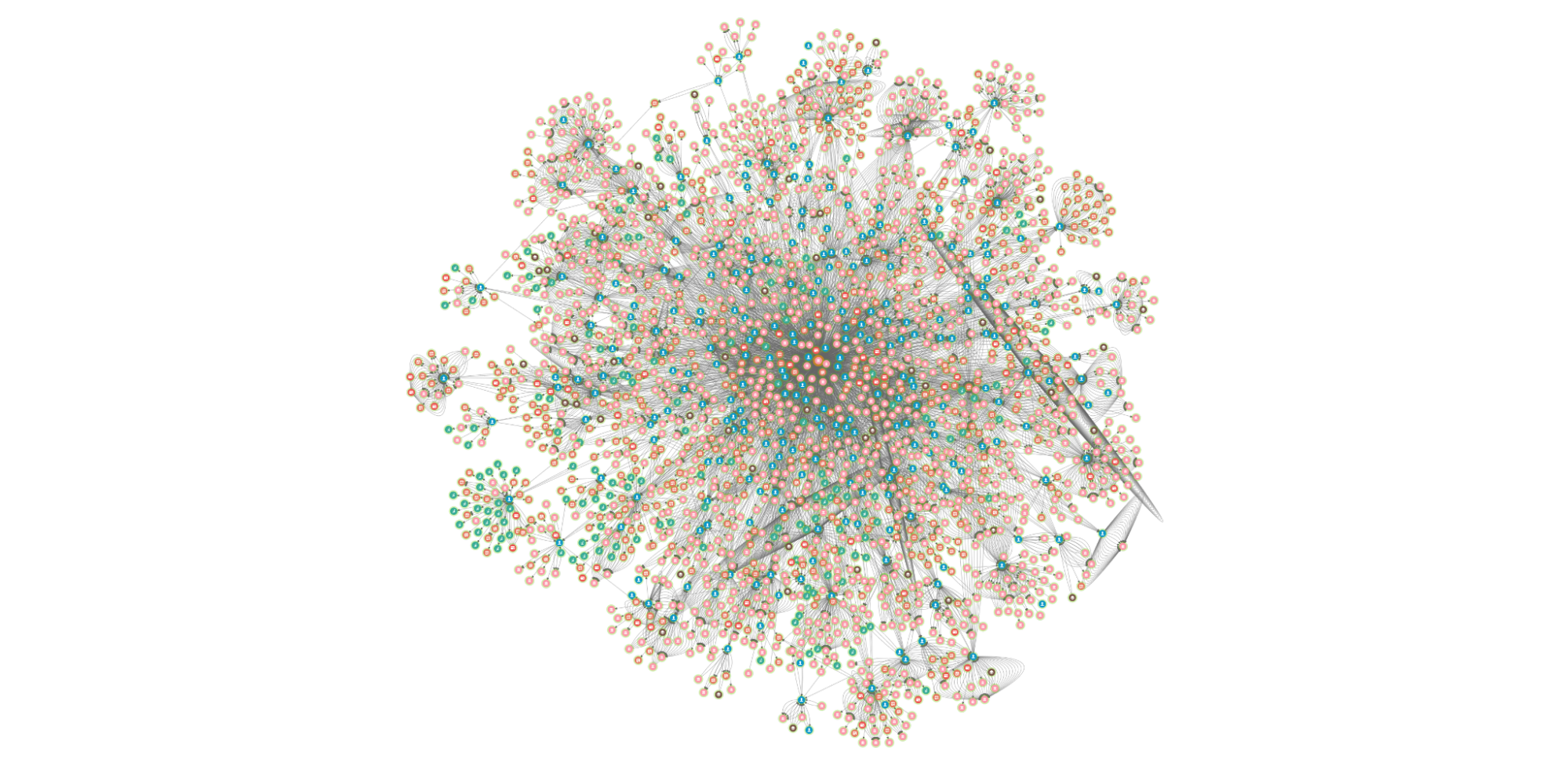
We are always looking for ways to improve fraud investigation methods and stay one step ahead of our ever-growing fraudsters. In the introductory blog of this series, we’ve mentioned experimenting with a set of Graph Network technologies, including Graph Visualisation.
In this post, we will introduce our Graph Visualisation Platform and briefly illustrate how it makes fraud investigations easier and more effective.
If you’re a fan of crime shows, you would have come across scenes like a detective putting together evidence, such as pictures, notes and articles, on a board and connecting them with thumb tacks and yarn. When you look at the board, it’s easy to see the relationships between the different pieces of evidence. That’s what graphs do, especially in fraud detection.
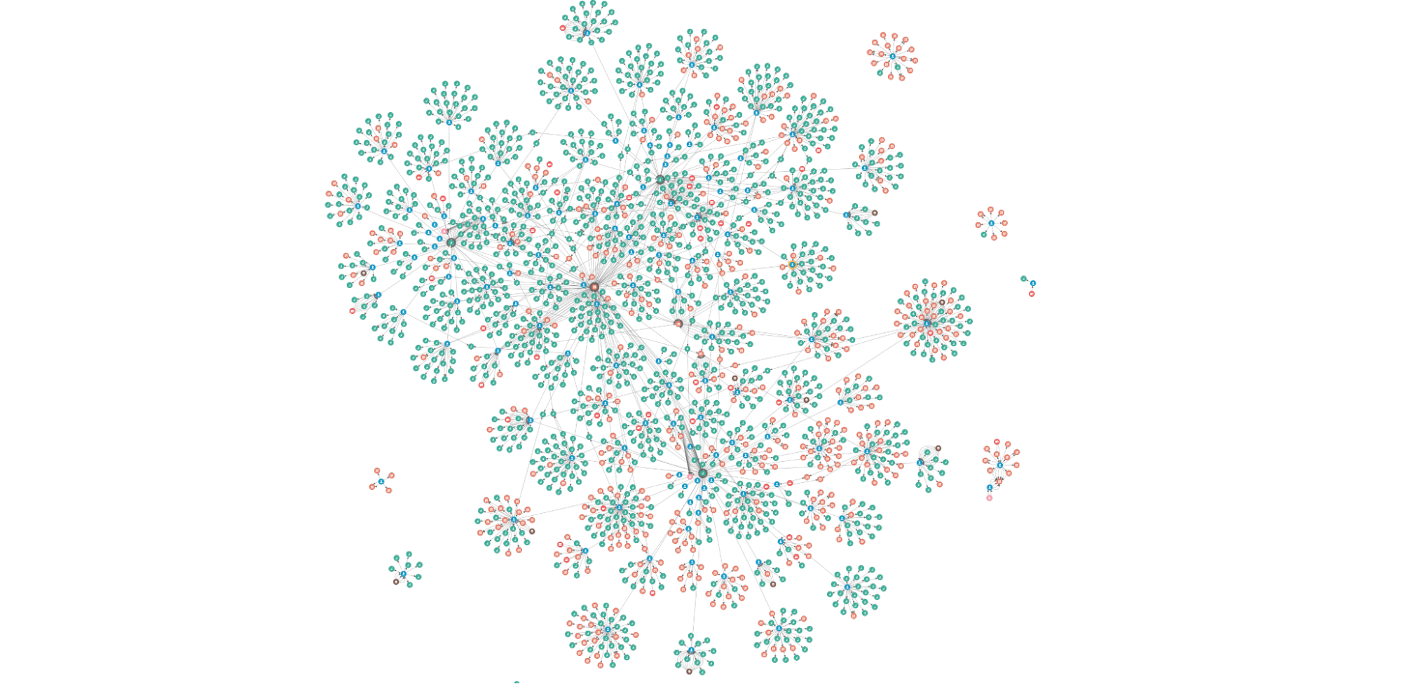
In the same way, while graph data is the raw material of an investigation, some of the most interesting relationships are often inferred rather than modelled directly in the data. Visualising these relationships can give a unique “big picture” of the data that is difficult or impossible to obtain with traditional relational tables and business intelligence tools.
On the other hand, graph visualisation enhances the quick identification of relationships and significant structures because it is an intuitive way to help detect patterns. Plus, the human brain processes visual information much faster; that’s where our Graph Visualisation platform comes in.
Graph Visualisation platform is a full-featured investigation platform that can reveal hidden connections and context in data by transforming raw records into highly visual and interactive maps. From there, investigators can grab any data point and quickly see relationships, patterns, and anomalies, and if necessary, drill down to investigate further.
This is all done without writing a manual query, switching between anti-fraud systems, or having to think about data science! These are some of the interactions on the platform that easily make anomalies or relevant patterns stand out.
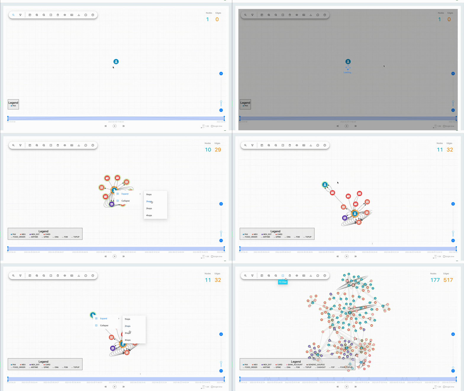
To date, we have over three billion nodes and edges in our storage system. It is not possible (nor necessary) to show all of the data at once. The platform allows the user to grab any data point and easily expand to view the relationships.
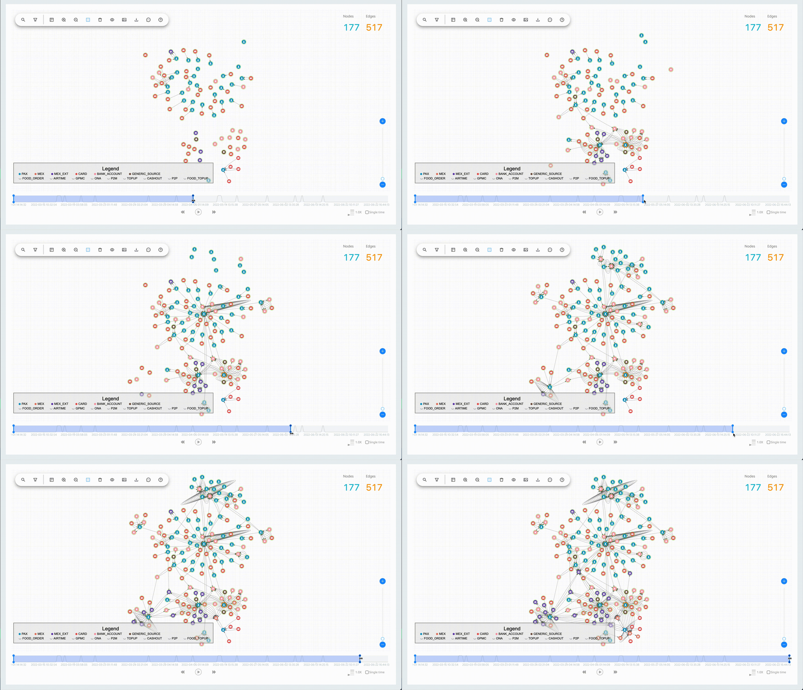
The Graph Visualisation platform’s interactive time filter lets you see temporal relationships within your data and clearly reveals the chronological progression of events. You can start with a specific time of interest, track everything that happens after, then quickly focus on the time and relationships that matter most.
Here are a few examples of how the Graph Visualisation platform facilitates fraud investigations.
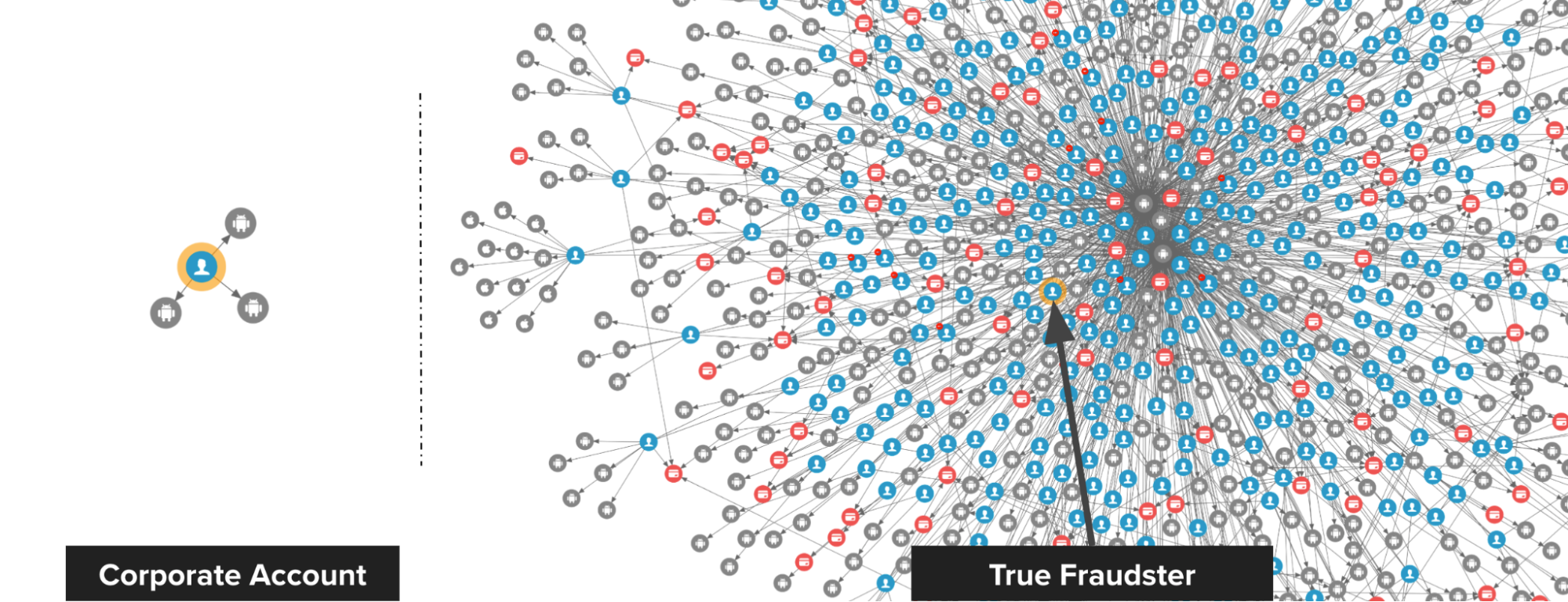
The following image shows the difference between a true fraudster and a falsely identified one. On the left, we have a Grab rental corporate account that was falsely detected by a fraud rule. Upon review, we discovered that there is no suspicious connection to this account, thus the account got unblocked.
On the right, we have a passenger that was blocked by the system and they appealed. Investigations showed that the passenger is, in fact, part of an extremely dense device-sharing network, so we maintained our decision to block.
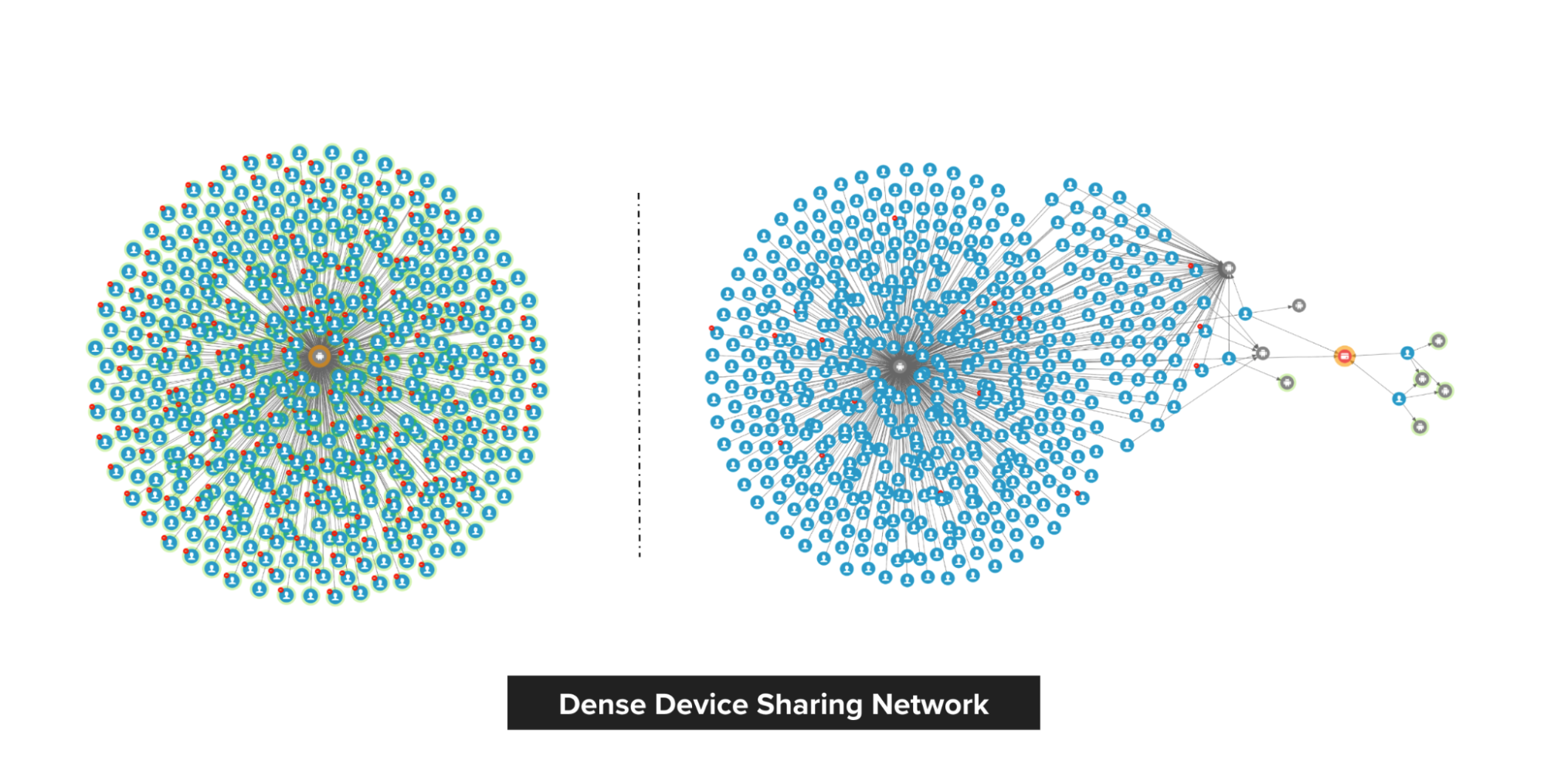
Fraudsters tend to share physical resources to maximise their revenue. With our Graph Visualisation platform, you can see exactly how this pattern looks like. The image below shows a device that is shared by a lot of fraudsters.
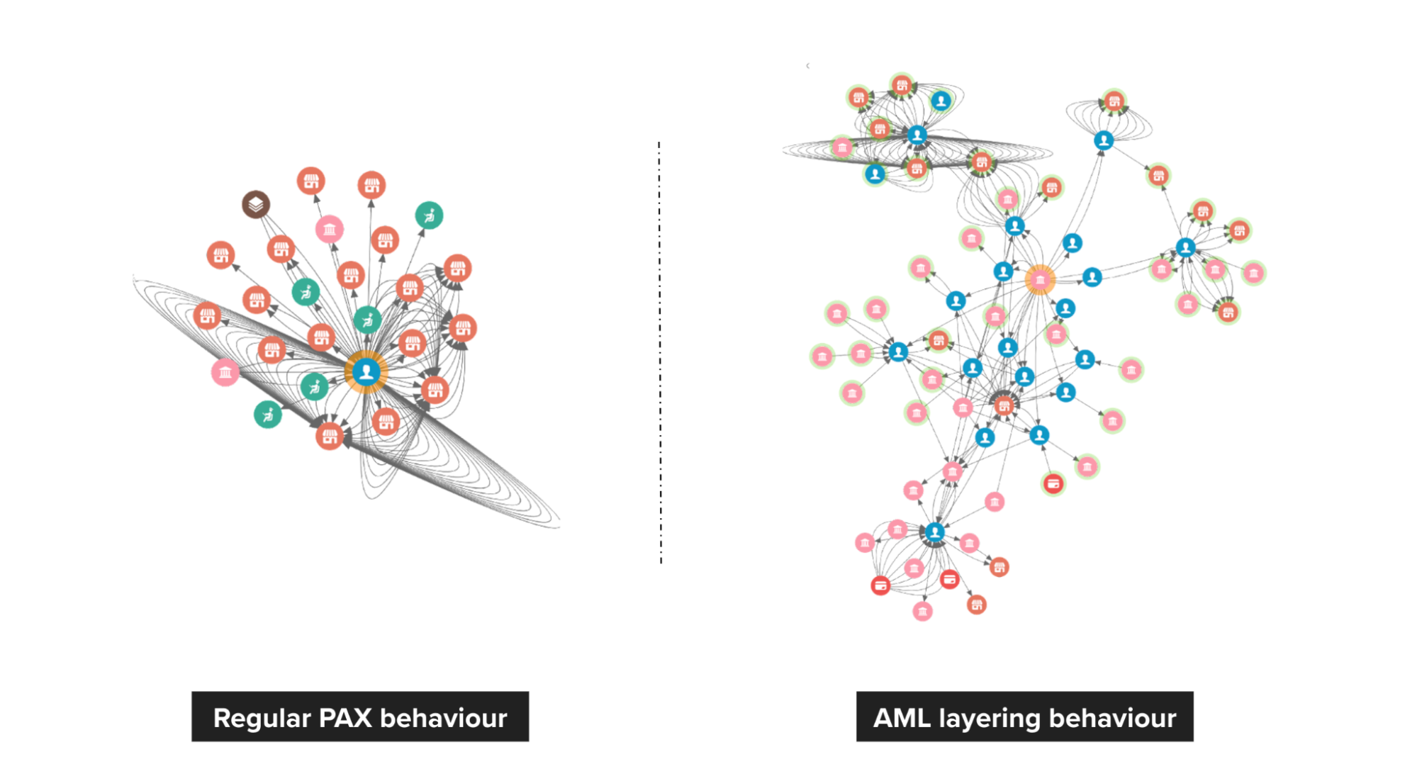
On the left, we see a pattern of healthy spending on Grab. However, on the right, we can see that passengers are highly connected, and it has frequent large amount transfers to other payment providers.
Graph Visualisation is an intuitive way to investigate suspicious connections and potential patterns of crime. Investigators can directly interact with any data point to get the details they need and literally view the relationships in the data to make fast, accurate, and defensible decisions.
While fraud detection is a good use case for Graph Visualisation, it’s not the only possibility. Graph Visualisation can help make anything more efficient and intelligent, especially if you have highly connected data.
In the next part of this blog series, we will talk about the Graph service platform and the importance of building graph services with graph databases. Check out the other articles in this series:
Grab is the leading superapp platform in Southeast Asia, providing everyday services that matter to consumers. More than just a ride-hailing and food delivery app, Grab offers a wide range of on-demand services in the region, including mobility, food, package and grocery delivery services, mobile payments, and financial services across 428 cities in eight countries.
Powered by technology and driven by heart, our mission is to drive Southeast Asia forward by creating economic empowerment for everyone. If this mission speaks to you, join our team today!
Post Syndicated from original https://lwn.net/Articles/899281/
On the first day of the 2022 Linux
Security Summit North America (LSSNA) in Austin, Texas, Stéphane Graber
and Christian Brauner gave a presentation on using system-call interception
for container security purposes. The idea is to allow unprivileged
containers, those without elevated privileges on the host, to still
accomplish their tasks, some of which require privileges. A fair amount of
work has been done to make this
viable, but there is still more to do.
Post Syndicated from original https://lwn.net/Articles/899404/
CODE
22.05 has been released; this is the “developer edition” of the
Collabora Online offering formerly known as LibreOffice Online.
CODE 22.05 is preceding the next major release of our long-term
supported business suite Collabora Online. This free developer
version includes all features and enhancements that will be
available in our enterprise version, expected later in July. The
CODE releases allow every interested user to learn and test new
features on an early stage.
New features include support for external grammar checkers, the ability to
have 16,000 columns in a spreadsheet (which is evidently useful to
somebody), sparkline plots, support for WebP graphics, and more.
Post Syndicated from Sheila Busser original https://aws.amazon.com/blogs/compute/leveraging-aws-nitro-enclaves-to-perform-computation-of-multiple-sensitive-datasets/
This blog post is written by, Jeff Wisman, Principal Solutions Architect and Andrew Lee, Solutions Architect.
Many organizations have sensitive datasets that they do not want to share with others because of stringent security and compliance requirements. However, they would still like to use each other’s data to perform processing and aggregation. For example, B2B (business to business) companies often want to augment their customer information dataset with additional demographic or psychographic signals. This enrichment of data is often done by one party sending customer information to be matched against another party’s data universe. Naturally, privacy and the revealing of business-critical customer information to an external entity is a major concern here. In this blog, we present a solution where multiple parties can choose to give an isolated compute environment access to their encrypted data to be decrypted and processed in a secure way using AWS Nitro Enclaves.
Designing and building your own secure private computing solution can be challenging, with few out-of-the-box solutions. Our sample application uses Nitro Enclaves, which support the creation of an isolated execution environment called an enclave and a cryptographic attestation process for generating and validating the enclave’s identity. The attestation process makes it possible to ensure only authorized code is running, as well as integration with the AWS Key Management Service (AWS KMS), so that only enclaves that you choose can access sensitive data. Nitro Enlaves enables customers to focus more on their application instead of worrying about integration with external services. While many enterprise use cases involve complex datasets, we’ll use a hypothetical scenario to learn the fundamentals of how this works. The example proof of concept (POC) application will be centered around a third-party bidding service for real estate transactions. Buyers will submit encrypted bids to the application. Once all the bids have been entered, the application will decrypt the bids, determine the highest bidder, and return a result without disclosing the actual bid amounts to any party.
The POC will be deployed across three AWS accounts, one each for buyer-1, buyer-2, and the bidding service. The bidding service will be run in an enclave on the bidding service’s account.
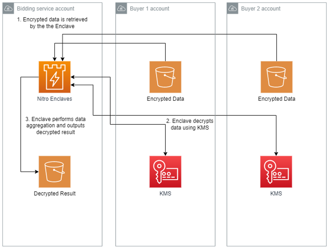
Let’s take a deeper dive into the steps involved in implementing this POC. To deploy the POC to your environment, follow the instructions in the AWS Nitro Enclaves Bidding Service GitHub project.
The first step is for the bidding service to launch the parent instance that will host the enclave. Refer to Launch the parent instance for more information about this process. The two real estate buyers, which we will call buyer-1 and buyer-2, will need to review the application code of the enclave application and agree that their data will not be exposed outside the enclave. Once they agree on the code, the bidding service generates the enclave image and a set of measurements as part of the attestation process. The buyers should also perform this process to ensure that the enclave image was generated and its measurements are from the agreed-upon application code. During the generation process, a unique set of measurements is taken of the application, which will make up its identity. When the enclave makes a request to decrypt data with AWS KMS, those measurements will be included in an attestation document to prove the enclave’s identity. Access policies in AWS KMS can then grant access to that identity. An example of a set of measurements is shown here:
Enclave Image successfully created.
{ "Measurements": { "HashAlgorithm": "Sha384 { ... }",
"PCR0":"287b24930a9f0fe14b01a71ecdc00d8be8fad90f9834d547158854b8279c74095c43f8d7f047714e98deb7903f20e3dd",
"PCR1":"aca6e62ffbf5f7deccac452d7f8cee1b94048faf62afc16c8ab68c9fed8c38010c73a669f9a36e596032f0b973d21895",
"PCR2":"0315f483ae1220b5e023d8c80ff1e135edcca277e70860c31f3003b36e3b2aaec5d043c9ce3a679e3bbd5b3b93b61d6f"
} }Each buyer will create an AWS KMS key and use that key to encrypt their bids. The encrypted bids will be stored in their respective S3 buckets. Because AWS KMS integrates with Nitro Enclaves to provide built-in attestation support, each buyer can add the PCR values generated earlier as a condition to their respective AWS KMS key policies. This will ensure that only the enclave application code agreed upon by both buyers will have access to utilize the keys for decryption. The following is an example of a KMS key policy with PCR values as a condition:
{
  "Version": "2012-10-17",
  "Id": "key-default-1",
  "Statement": [{
    "Sid": "Enable decrypt from enclave",
    "Effect": "Allow",
    "Principal": < PARENT INSTANCE ROLE ARN > ,
    "Action": "kms:Decrypt",
    "Resource": "",
    "Condition": {
      "StringEqualsIgnoreCase": {
        "kms:RecipientAttestation:ImageSha384": "<PCR0 VALUE FROM BUILDING ENCLAVE IMAGE>",
        "kms:RecipientAttestation:PCR1":"<PCR1 VALUE FROM BUILDING ENCLAVE IMAGE>",
        "kms:RecipientAttestation:PCR2":"<PCR2 VALUE FROM BUILDING ENCLAVE IMAGE>"
      }
    }
  }]
}
The previous example only shows a key policy that uses PCR0, PCR1, and PCR2. You can further scope down the permissions by adding additional PCR values, for instance, role, parent instance ID, and a signing certificate for the enclave image. Refer to the AWS Nitro Enclaves User Guide for more details about PCR values.
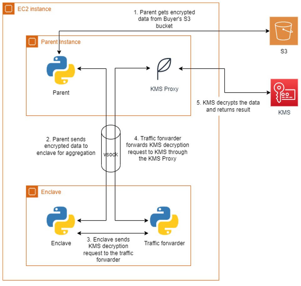
The bidding service will run the enclave image generated earlier on the parent instance. The application runs as two parts, one part on the parent instance and another in the enclave. Communication between the parent and the enclave is done through a vsock connection. An AWS KMS proxy is also used on the parent to allow communication between the enclave and AWS KMS for decrypting data. The parent application will retrieve the encrypted bids from each buyer’s S3 bucket and send them to the enclave. The enclave will decrypt the data using both buyers’ AWS KMS keys and present attestation documents signed by the Nitro Hypervisor. AWS KMS will validate that the PCR values in the attestation documents match the key policy before performing the decryption. The decryption event will be logged in AWS CloudTrail for auditing purposes. Once the encrypted bids are decrypted, the values are compared, and the winning buyer is recorded in the result. The unencrypted result is then returned to the parent and written to an S3 bucket in the bidding service’s account. A diagram of this process is shown in Figure 2.
Be sure you delete all the resources that were created when following the included Github project:
In this blog post, we introduced a sample POC utilizing Nitro Enclaves to allow a bidding service to process two parties’ encrypted data without revealing their data to any party. We did this by ensuring access to sensitive data is only allowed from an application running within an enclave. With the straightforward integration of AWS KMS and the attestation process, customers can quickly develop applications on Nitro Enclaves that can enable computing on encrypted datasets from multiple accounts. For more information on AWS Nitro Enclaves, see the official product documentation or the introductory videos on YouTube.
Post Syndicated from Jeff Hostetler original https://github.blog/2022-06-29-improve-git-monorepo-performance-with-a-file-system-monitor/
If you have a monorepo, you’ve probably already felt the pain of slow Git commands, such as git status and git add. These commands are slow because they need to search the entire worktree looking for changes. When the worktree is very large, Git needs to do a lot of work.
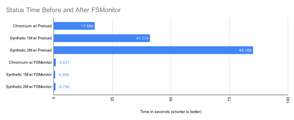
The Git file system monitor (FSMonitor) feature can speed up these commands by reducing the size of the search, and this can greatly reduce the pain of working in large worktrees. For example, this chart shows status times dropping to under a second on three different large worktrees when FSMonitor is enabled!
In this article, I want to talk about the new builtin FSMonitor git fsmonitor--daemon added in Git version 2.37.0. This is easy to set up and use since it is “in the box” and does not require any third-party tooling nor additional software. It only requires a config change to enable it. It is currently available on macOS and Windows.
To enable the new builtin FSMonitor, just set core.fsmonitor to true. A daemon will be started automatically in the background by the next Git command.
FSMonitor works well with core.untrackedcache, so we’ll also turn it on for the FSMonitor test runs. We’ll talk more about the untracked-cache later.
$ time git status
On branch main
Your branch is up to date with 'origin/main'.

It took 5.25 seconds to enumerate untracked files. 'status -uno'
may speed it up, but you have to be careful not to forget to add
new files yourself (see 'git help status').
nothing to commit, working tree clean

real    0m17.941s
user    0m0.031s
sys     0m0.046s

$ git config core.fsmonitor true
$ git config core.untrackedcache true

$ time git status
On branch main
Your branch is up to date with 'origin/main'.

It took 6.37 seconds to enumerate untracked files. 'status -uno'
may speed it up, but you have to be careful not to forget to add
new files yourself (see 'git help status').
nothing to commit, working tree clean

real    0m19.767s
user    0m0.000s
sys     0m0.078s

$ time git status
On branch main
Your branch is up to date with 'origin/main'.

nothing to commit, working tree clean

real    0m1.063s
user    0m0.000s
sys     0m0.093s

$ git fsmonitor--daemon status
fsmonitor-daemon is watching 'C:/work/chromium'
_Note that when the daemon first starts up, it needs to synchronize with the state of the index, so the next git status command may be just as slow (or slightly slower) than before, but subsequent commands should be much faster.
In this article, I’ll introduce the new builtin FSMonitor feature and explain how it improves performance on very large worktrees.
How FSMonitor improves performance
Git has a “What changed while I wasn’t looking?” problem. That is, when you run a command that operates on the worktree, such as git status, it has to discover what has changed relative to the index. It does this by searching the entire worktree. Whether you immediately run it again or run it again tomorrow, it has to rediscover all of that same information by searching again. Whether you edit zero, one, or a million files in the mean time, the next git status command has to do the same amount of work to rediscover what (if anything) has changed.
The cost of this search is relatively fixed and is based upon the number of files (and directories) present in the worktree. In a monorepo, there might be millions of files in the worktree, so this search can be very expensive.
What we really need is a way to focus on the changed files without searching the entire worktree.
How FSMonitor works
FSMonitor is a long-running daemon or service process.
git status.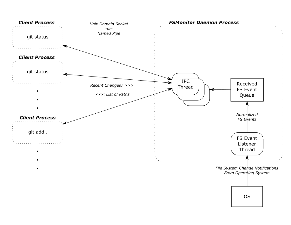
FSMonitor must continuously watch the worktree to have a complete view of all file system changes, especially ones that happen between Git commands. So it must be a long-running daemon or service process and not associated with an individual Git command instance. And thus, it cannot be a traditional Git hook (child) process. This design does allow it to service multiple (possibly concurrent) Git commands.
FSMonitor Synchronization
FSMonitor has the concept of a “token”:
git status writes the received token into the index with other FSMonitor data before it exits. The next git status command reads the previous token (along with the other FSMonitor data) and asks FSMonitor what changed since the previous token.
Earlier, I said a token is like a timestamp, but it also includes other fields to prevent incomplete responses:
In both cases, a normal response from the daemon would be incomplete because of gaps in the data. Instead, the daemon responds with a trivial (“assume everything was changed”) response and a new token. This will cause the current Git client command to do a regular scan of the worktree (as if FSMonitor were not enabled), but let future client commands be fast again.
Types of files in your worktree
When git status examines the worktree, it looks for tracked, untracked, and ignored files.

Tracked files are files under version control. These are files that Git knows about. These are files that Git will create in your worktree when you do a git checkout. The file in the worktree may or may not match the version listed in the index. When different, we say that there is an unstaged change. (This is independent of whether the staged version matches the version referenced in the HEAD commit.)
Untracked files are just that: untracked. They are not under version control. Git does not know about them. They may be temporary files or new source files that you have not yet told Git to care about (using git add).
Ignored files are a special class of untracked files. These are usually temporary files or compiler-generated files. While Git will ignore them in commands like git add, Git will see them while searching the worktree and possibly slow it down.
Normally, git status does not print ignored files, but we’ll turn it on for this example so that we can see all four types of files.
$ git status --ignored
On branch master
Changes to be committed:
  (use "git restore --staged <file>..." to unstage)
    modified:   README

Changes not staged for commit:
  (use "git add <file>..." to update what will be committed)
  (use "git restore <file>..." to discard changes in working directory)
    modified:   README
    modified:   main.c

Untracked files:
  (use "git add <file>..." to include in what will be committed)
    new-file.c

Ignored files:
  (use "git add -f <file>..." to include in what will be committed)
    new-file.obj
The expensive worktree searches
During the worktree search, Git treats tracked and untracked files in two distinct phases. I’ll talk about each phase in detail in later sections.
There is a third phase where Git compares the index and the HEAD commit to look for staged changes, but this phase is very fast, because it is inspecting internal data structures that are designed for this comparision. It avoids the significant number of system calls that are required to inspect the worktree, so we won’t worry about it here.
A detailed example
The chart in the introduction showed status times before and after FSMonitor was enabled. Let’s revisit that chart and fill in some details.
I collected performance data for git status on worktrees from three large repositories. There were no modified files, and git status was clean.
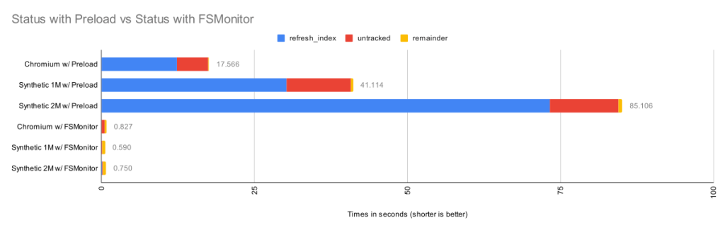
Here we can see that when FSMonitor is not present, the commands took from 17 to 85 seconds. However, when FSMonitor was enabled the commands took less than 1 second.
Each bar shows the total run time of the git status commands. Within each bar, the total time is divided into parts based on performance data gathered by Git’s trace2 library to highlight the important or expensive steps within the commands.
| Worktree | Files | refresh_index
with Preload |
Untracked
without Untracked-Cache |
Remainder | Total |
| Chromium | 393K | 12.3s | 5.1s | 0.16s | 17.6s |
| Synthetic 1M | 1M | 30.2s | 10.5s | 0.36s | 41.1s |
| Synthetic 2M | 2M | 73.2s | 11.2s | 0.64s | 85.1s |
The top three bars are without FSMonitor. We can see that most of the time was spent in the refresh_index and untracked columns. I’ll explain what these are in a minute. In the remainder column, I’ve subtracted those two from the total run time. This portion barely shows up on these bars, so the key to speeding up git status is to attack those two phases.
The bottom three bars on the above chart have FSMonitor and the untracked-cache enabled. They show a dramatic performance improvement. On this chart these bars are barely visible, so let’s zoom in on them.
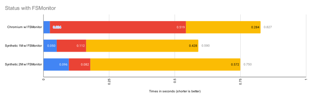
This chart rescales the FSMonitor bars by 100X. The refresh_index and untracked columns are still present but greatly reduced thanks to FSMonitor.
| Worktree | Files | refresh_index
with FSMonitor |
Untracked
with FSMonitor and Untracked-Cache |
Remainder | Total |
| Chromium | 393K | 0.024s | 0.519s | 0.284s | 0.827s |
| Synthetic 1M | 1M | 0.050s | 0.112s | 0.428s | 0.590s |
| Synthetic 2M | 2M | 0.096s | 0.082s | 0.572s | 0.750s |
This is bigger than just status
So far I’ve only talked about git status, since it is the command that we probably use the most and are always thinking about when talking about performance relative to the state and size of the worktree. But it is just one of many affected commands:
git diff does the same search, but uses the changed files it finds to print a difference in the worktree and your index.git add . does the same search, but it stages each changed file it finds.git restore and git checkout do the same search to decide the files to be replaced.So, for simplicity, I’ll just talk about git status, but keep in mind that this approach benefits many other commands, since the cost of actually staging, overwriting, or reporting the change is relatively trivial by comparison — the real performance cost in these commands (as the above charts show) is the time it takes to simply find the changed files in the worktree.
Phase 1: refresh_index
The index contains an “index entry” with information for each tracked file. The git ls-files command can show us what that list looks like. I’ll truncate the output to only show a couple of files. In a monorepo, this list might contain millions of entries.
$ git ls-files --stage --debug
[...]
100644 7ce4f05bae8120d9fa258e854a8669f6ea9cb7b1 0   README.md
  ctime: 1646085519:36302551
  mtime: 1646085519:36302551
  dev: 16777220 ino: 180738404
  uid: 502  gid: 20
  size: 3639    flags: 0
[...]
100644 5f1623baadde79a0771e7601dcea3c8f2b989ed9 0   Makefile
  ctime: 1648154224:994917866
  mtime: 1648154224:994917866
  dev: 16777221 ino: 182328550
  uid: 502  gid: 20
  size: 110149  flags: 0
[...]
Scanning tracked files for unstaged changes
Let’s assume at the beginning of refresh_index that all index entries are “unmarked” — meaning that we don’t know yet whether or not the worktree file contains an unstaged change. And we “mark” an index entry when we know the answer (either way).

To determine if an individual tracked file has an unstaged change, it must be “scanned”. That is, Git must read, clean, hash the current contents of the file, and compare the computed hash value with the hash value stored in the index. If the hashes are the same, we mark the index entry as “valid”. If they are different, we mark it as an unstaged change.
In theory, refresh_index must repeat this for each tracked file in the index.
As you can see, each individual file that we have to scan will take time and if we have to do a “full scan”, it will be very slow, especially if we have to do it for millions of files. For example, on the Chromium worktree, when I forced a full scan it took almost an hour.
| Worktree | Files | Full Scan |
| Chromium | 393K | 3072s |
refresh_index shortcuts
Since doing a full scan of the worktree is so expensive, Git has developed various shortcuts to avoid scanning whenever possible to increase the performance of refresh_index.
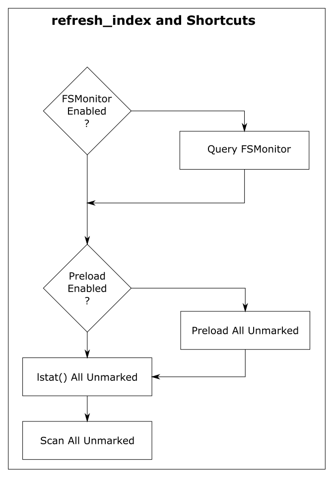
For discussion purposes, I’m going to describe them here as independent steps rather than somewhat intertwined steps. And I’m going to start from the bottom, because the goal of each shortcut is to look at unmarked index entries, mark them if they can, and make less work for the next (more expensive) step. So in a perfect world, the final “full scan” would have nothing to do, because all of the index entries have already been marked, and there are no unmarked entries remaining.
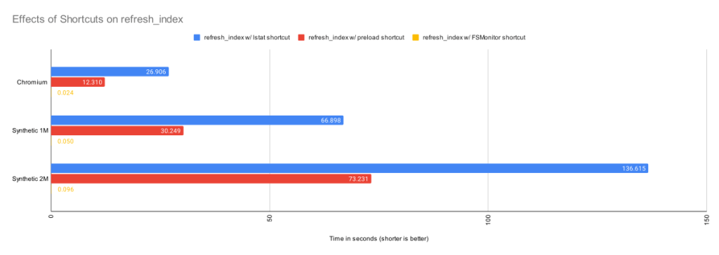
In the above chart, we can see the cummulative effects of these shortcuts.
Shortcut: refresh_index with lstat()
The “lstat() shortcut” was created very early in the Git project.
To avoid actually scanning every tracked file on every git status command, Git relies on a file’s last modification time (mtime) to tell when a file was last changed. File mtimes are updated when files are created or edited. We can read the mtime using the lstat() system call.
When Git does a git checkout or git add, it writes each worktree file’s current mtime into its index entry. These serve as the reference mtimes for future git status commands.
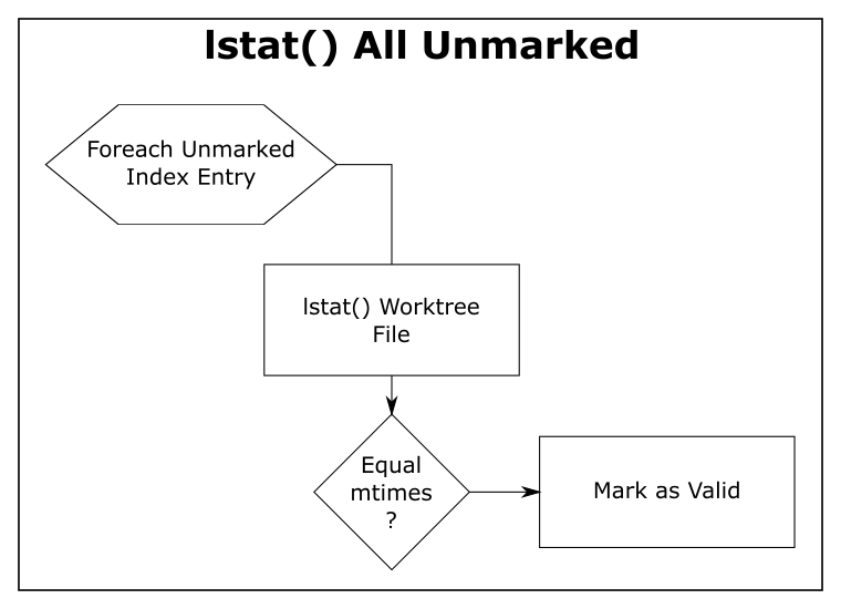
Then, during a later git status, Git checks the current mtime against the reference mtime (for each unmarked file). If they are identical, Git knows that the file content hasn’t changed and marks the index entry valid (so that the next step will avoid it). If the mtimes are different, this step leaves the index entry unmarked for the next step.
| Worktree | Files | refresh_index with lstat()
|
| Chromium | 393K | 26.9s |
| Synthetic 1M | 1M | 66.9s |
| Synthetic 2M | 2M | 136.6s |
The above table shows the time in seconds taken to call lstat() on every file in the worktree. For the Chromium worktree, we’ve cut the time of refresh_index from 50 minutes to 27 seconds.
Using mtimes is much faster than always scanning each file, but Git still has to lstat() every tracked file during the search, and that can still be very slow when there are millions of files.
In this experiment, there were no modifications in the worktree, and the index was up to date, so this step marked all of the index entries as valid and the “scan all unmarked” step had nothing to do. So the time reported here is essentially just the time to call lstat() in a loop.
This is better than before, but even though we are only doing an lstat(), git status is still spending more than 26 seconds in this step. We can do better.
Shortcut: refresh_index with preload
The core.preloadindex config option is an optional feature in Git. The option was introduced in version 1.6 and was enabled by default in 2.1.0 on platforms that support threading.
This step partitions the index into equal-sized chunks and distributes it to multiple threads. Each thread does the lstat() shortcut on their partition. And like before, index entries with different mtimes are left unmarked for the next step in the process.
The preload step does not change the amount of file scanning that we need to do in the final step, it just distributes the lstat() calls across all of your cores.
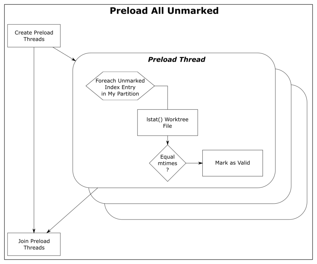
| Worktree | Files | refresh_index with Preload |
| Chromium | 393K | 12.3s |
| Synthetic 1M | 1M | 30.2s |
| Synthetic 2M | 2M | 73.2s |
With the preload shortcut git status is about twice as fast on my 4-core Windows laptop, but it is still expensive.
Shortcut: refresh_index with FSMonitor
When FSMonitor is enabled:
git fsmonitor--daemon is started in the background and listens for file system change notification events from the operating system for files within the worktree. This includes file creations, deletions, and modifications. If the daemon gets an event for a file, that file probably has an updated mtime. Said another way, if a file mtime changes, the daemon will get an event for it.git status data between git status commands. The extension contains an FSMonitor token and a bitmap listing the files that were marked valid by the previous git status command (and relative to that token).git status command will use this bitmap to initialize the marked state of the index entries. That is, the previous Git command saved the marked state of the index entries in the bitmap and this command restores them — rather than initializing them all as unmarked.At this point, all of the unchanged files should be marked valid. Only files that may have changed should be unmarked. This sets up the next shortcut step to have very little to do.
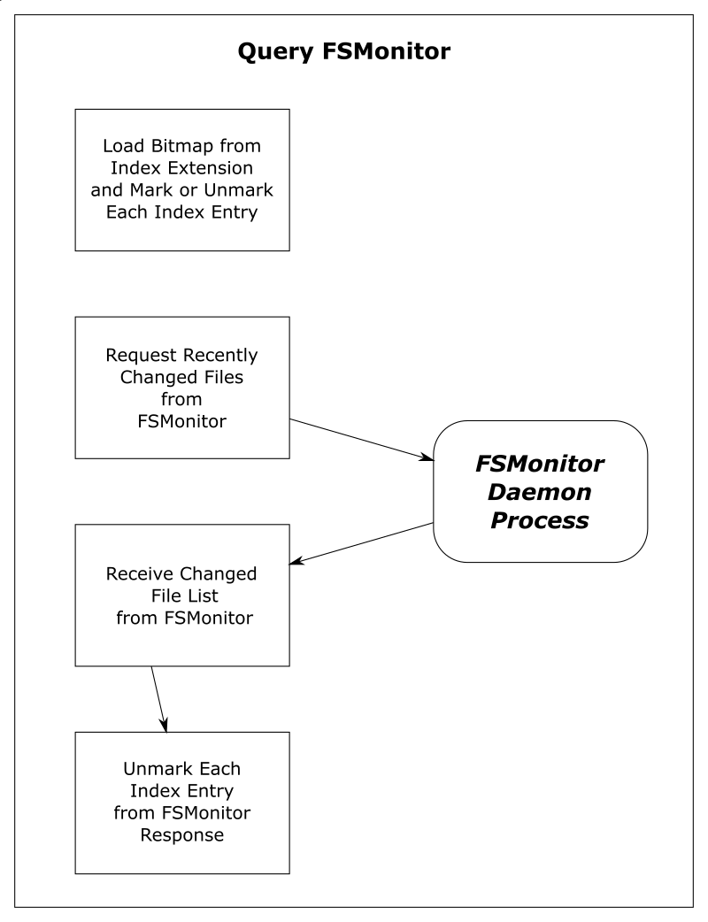
| Worktree | Files | Query FSMonitor | refresh_index with FSMonitor |
| Chromium | 393K | 0.017s | 0.024s |
| Synthetic 1M | 1M | 0.002s | 0.050s |
| Synthetic 2M | 2M | 0.002s | 0.096s |
This table shows that refresh_index is now very fast since we don’t need to any searching. And the time to request the list of files over IPC is well worth the complex setup.
Phase 2: untracked
The “untracked” phase is a search for anything in the worktree that Git does not know about. These are files and directories that are not under version control. This requires a full search of the worktree.
Conceptually, this looks like:
.gitignore pattern matching rules. If a match is found, then the pathname is an ignored file and is omitted from the list. This pattern matching can be very expensive if there are lots of rules.This search can be very expensive on monorepos and frequently leads to the following advice message:
$ git status
On branch main
Your branch is up to date with 'origin/main'.

It took 5.12 seconds to enumerate untracked files. 'status -uno'
may speed it up, but you have to be careful not to forget to add
new files yourself (see 'git help status').
nothing to commit, working tree clean
Normally, the complete discovery of the set of untracked files must be repeated for each command unless the [core.untrackedcache](https://git-scm.com/docs/git-config#Documentation/git-config.txt-coreuntrackedCache) feature is enabled.
The untracked-cache
The untracked-cache feature adds an extension to the index that remembers the results of the untracked search. This includes a record for each subdirectory, its mtime, and a list of the untracked files within it.
With the untracked-cache enabled, Git still needs to lstat() every directory in the worktree to confirm that the cached record is still valid.
If the mtimes match:
opendir() and readdir() to enumerate the files within the directory,If the mtimes don’t match:
lstat() on each file or subdirectory within the directory to determine if it is a file or directory and possibly invalidate untracked-cache entries for any subdirectories.How FSMonitor helps the untracked-cache
When FSMonitor is also enabled, we can avoid the lstat() calls, because FSMonitor tells us the set of directories that may have an updated mtime, so we don’t need to search for them.
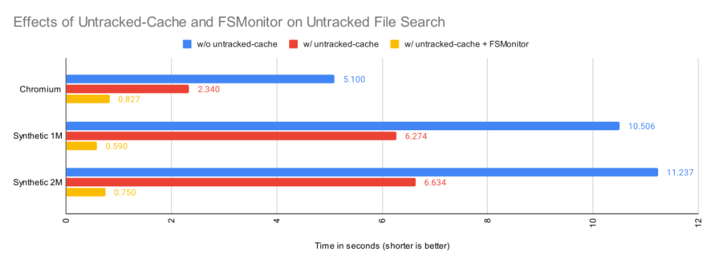
| Worktree | Files | Untracked
without Untracked-Cache |
Untracked
with Untracked-Cache |
Untracked
with Untracked-Cache and FSMonitor |
| Chromium | 393K | 5.1s | 2.3s | 0.83s |
| Synthetic 1M | 1M | 10.5s | 6.3s | 0.59s |
| Synthetic 2M | 2M | 11.2s | 6.6s | 0.75s |
By itself, the untracked-cache feature gives roughly a 2X speed up in the search for untracked files. Use both the untracked-cache and FSMonitor, and we see a 10X speedup.
A note about ignored files
You can improve Git performance by not storing temporary files, such as compiler intermediate files, inside your worktree.
During the untracked search, Git first eliminates the tracked files from the candidate untracked list using the index. Git then uses the .gitignore pattern matching rules to eliminate the ignored files. Git’s performance will suffer if there are many rules and/or many temporary files.
For example, if there is a *.o for every source file and they are stored next to their source files, then every build will delete and recreate one or more object files and cause the mtime on their parent directories to change. Those mtime changes will cause git status to invalidate the corresponding untracked-cache entries and have to re-read and re-filter those directories — even if no source files actually changed. A large number of such temporary and uninteresting files can greatly affect the performance of these Git commands.
Keeping build artifacts out of your worktree is part of the philosophy of the Scalar Project. Scalar introduced Git tooling to help you keep your worktree in <repo-name>/src/ to make it easier for you to put these other files in <repo-name>/bin/ or <repo-name>/packages/, for example.
A note about sparse checkout
So far, we’ve talked about optimizations to make Git work smarter and faster on worktree-related operations by caching data in the index and in various index extensions. Future commands are faster, because they don’t have to rediscover everything and therefore can avoid repeating unnecessary or redundant work. But we can only push that so far.
The Git sparse checkout feature approaches worktree performance from another angle. With it, you can ask Git to only populate the files that you need. The parts that you don’t need are simply not present. For example, if you only need 10% of the worktree to do your work, why populate the other 90% and force Git to search through them on every command?
Sparse checkout speeds the search for unstaged changes in refresh_index because:
refresh_index can completely ignore them.git checkout with the skip-worktree bit, so they are never in an “unmarked” state. So those index entries are excluded from all of the refresh_index loops.Sparse checkout speeds the search for untracked files because:
External file system monitors
So far we have only talked about Git’s builtin FSMonitor feature. Clients use the simple IPC interface to communicate directly with git fsmonitor--daemon over a Unix domain socket or named pipe.
However, Git added support for an external file system monitor in version 2.16.0 using the core.fsmonitor hook. Here, clients communicate with a proxy child helper process through the hook interface, and it communicates with an external file system monitor process.
Conceptually, both types of file system monitors are identical. They include a long-running process that listens to the file system for changes and are able to respond to client requests for a list of recently changed files and directories. The response from both are used identically to update and modify the refresh_index and untracked searches. The only difference is in how the client talks to the service or daemon.
The original hook interface was useful, because it allowed Git to work with existing off-the-shelf tools and allowed the basic concepts within Git to be proven relatively quickly, confirm correct operation, and get a quick speed up.
Hook protocol versions
The original 2.16.0 version of the hook API used protocol version 1. It was a timestamp-based query. The client would send a timestamp value, expressed as nanoseconds since January 1, 1970, and expect a list of the files that had changed since that timestamp.
Protocol version 1 has several race conditions and should not be used anymore. Protocol version 2 was added in 2.26.0 to address these problems.
Protocol version 2 is based upon opaque tokens provided by the external file system monitor process. Clients make token-based queries that are relative to a previously issued token. Instead of making absolute requests, clients ask what has changed since their last request. The format and content of the token is defined by the external file system monitor, such as Watchman, and is treated as an opaque string by Git client commands.
The hook protocol is not used by the builtin FSMonitor.
Using Watchman and the sample hook script
Watchman is a popular external file system monitor tool and a Watchman-compatible hook script is included with Git and copied into new worktrees during git init.
To enable it:
$ watchman watch .
{
    "version": "2022.01.31.00",
    "watch": "/Users/jeffhost/work/chromium",
    "watcher": "fsevents"
}
$ cp .git/hooks/fsmonitor-watchman.sample .git/hooks/query-watchman
$ git config core.fsmonitor .git/hooks/query-watchman
Using Watchman with a custom hook
The hook interface is not limited to running shell or Perl scripts. The included sample hook script is just an example implementation. Engineers at Dropbox described how they were able to speed up Git with a custom hook executable.
Final Remarks
In this article, we have seen how a file system monitor can speed up commands like git status by solving the “discovery” problem and eliminating the need to search the worktree for changes in every command. This greatly reduces the pain of working with monorepos.
This feature was created in two efforts:
Having both options available lets users choose the best solution for their needs.
Regardless of which type of file system monitor you use, it will help make your monorepos more usable.
Post Syndicated from The Atlantic original https://www.youtube.com/watch?v=sHd0DlrorAQ
Post Syndicated from Luca Mezzalira original https://aws.amazon.com/blogs/architecture/lets-architect-understanding-the-build-versus-buy-dilemma/
Vendor lock in happens when you commit to a specific technology and then don’t have the freedom to maintain full control of your applications. Even if you want to switch to another vendor, it’s not easy because of the financial investment, effort, and time needed to do so.
In the cloud computing, technology changes quickly, and vendor lock in can impact your business objectives. In this edition of Let’s Architect!, we show you how to avoid the risks of vendor lock in and examine when you should build or buy new software.
In this blog post, Gregor Hohpe shares some tips on how to avoid risks of vendor lock in. He advises to “build the software that differentiates your business and buy all else” and shows you how opportunity cost, an economic concept, plays major role in whether to build or buy software.

Which is the right option for your business: build or buy? Customers often ask this question. The answer is: it depends.
Moving to the cloud does not necessarily mean you are locked in to a cloud provider. Most cloud platforms offer you a pay as-you-go model with the flexibility to choose from a wide range of services and solutions such as serverless, DevOps, etc. However, having advanced and scalable technology products powering your business can help differentiate your core product. And, it can help you innovate faster and increase speed and agility. This blog post will help you choose the right path for you based on your business objectives.

In this blog post, Mark Schwartz shares his personal story. He talks about his role as the CIO of US Citizenship and Immigration Services and how he decided to migrate their workloads to the cloud during his time there. He discusses some of his considerations in moving and some of the obstacles he encountered along the way.

Thanks for reading! See you in a couple of weeks when we discuss DevOps.
Post Syndicated from Talks at Google original https://www.youtube.com/watch?v=6Wf7pSfBFqE
Post Syndicated from BeardedTinker original https://www.youtube.com/watch?v=NNu-ED4YrzQ
Post Syndicated from Geographics original https://www.youtube.com/watch?v=YlDOJ4u4tUU
Post Syndicated from Benjamin Smith original https://aws.amazon.com/blogs/compute/introducing-the-new-aws-step-functions-workflows-collection/
Today, the AWS Serverless Developer Advocate team introduces the Step Functions Workflows Collection, a fresh experience that makes it easier to discover, deploy, and share Step Functions workflows.
Builders create Step Functions workflows to orchestrate multiple services into business-critical applications with minimal code. Customers were looking for opinionated templates that implement best practices for building serverless applications with Step Functions.
This blog post explains what Step Functions workflows are and what challenges they help solve. It shows how to use the new Step Functions workflows collection to find simple “building blocks”, reusable patterns, and example applications to help build your serverless applications with Step Functions.

Large serverless applications often comprise multiple decoupled resources. These are sometimes challenging to observe and discover errors. Step Functions is a low-code visual workflow service that helps solve this challenge. It provides instant visual understanding of an application, the services it integrates with, and any errors that might occur during execution.
Step Functions workflows comprise a sequence of steps where the output of one step passes on as input to the next. Step Functions can integrate with over 220 AWS services by using an AWS SDK integration task. This allows users to call AWS SDK actions directly without the need to write additional code.
Explore the Step Functions workflows collection to discover new workflows. The collection has three levels of workflows:
Workflows are also categorized by multiple use-cases, including data processing, SaaS integration, and security automation. Once you find a workflow that want to use in your application:

 The workflows collection currently supports deployable workflow templates defined with AWS Serverless Applications Model (AWS SAM) or the AWS Cloud Development Kit (AWS CDK)Structure of an AWS SAM template
AWS SAM is an open-source framework for building serverless applications. It provides shorthand syntax that makes it easier to build and deploy serverless applications. With only a few lines, you can define each resource using YAML or JSON.
An AWS SAM template can have serverless-specific resources or standard AWS CloudFormation resources. When you run sam deploy, sam transforms serverless resources into CloudFormation syntax.
Structure of an AWS CDK template
The AWS CDK provides another way to define your application resources using common programming languages. The CDK is an open source framework that you can use to model your applications. As with AWS SAM, when you run ‘npx cdk deploy –app ‘ts-node .’ , the CDK transforms the template into AWS CloudFormation syntax and creates the specified resources for you.
 ASL is a JSON-based, structured language for authoring Step Functions workflows. It enables developers to filter and manipulate data at various stages of a workflow state’s execution using paths. A path is a string beginning with $ that lets you identify and filter subsets of JSON text. Learning how to apply these filters helps to build efficient workflows with minimal state transitions.
The more advanced workflows in the collection show how to use intrinsic functions to manipulate payload data. Intrinsic functions are ASL constructs that help build and convert payloads without creating additional task state transitions. Use intrinsic functions in Task states within the ResultSelector field, or in a Pass state in either the Parameters or ResultSelector field. The Step Functions documentation shows examples of how to:


Continue building in your local IDE
For developers who prefer to build locally, the AWS Toolkit for VS Code enables you to define, visualize, and create your Step Functions workflows without leaving the VS Code. The toolkit also provides code snippets for seven different ASL state types and additional service integrations to speed up workflow development. To continue building locally with VS Code:

Anyone can contribute a workflow to the Step Functions workflows collection. GitHub can host new workflow files in the AWS workflows-collection repository, or in a pre-existing repository of your own.
To submit a workflow:

Additional guidance can be found in the repository’s PUBLISHING.md file.
Today, the AWS Serverless Developer Advocate team is launching a new Serverless Land experience called “The Step Functions workflows collection”. This helps builders search, deploy, and contribute example Step Functions workflows.
The workflows collection simplifies the Step Functions getting started experience, and also shows more advanced users how to apply best practices to their workflows. These examples consist of fundamental building blocks for workflows, common application patterns implemented as workflows, and end to end applications.
All Step Functions builders are invited to contribute to the collection. This is done by submitting a pull request to the Step Functions Workflows Collection GitHub repository. Each submission is reviewed by the Serverless Developer advocate for quality and relevancy before publishing.
You can now learn to use Step Functions with a new workshop called the AWS Step Functions Workshop. This self-paced tutorial teaches you how to use the primary features of Step Functions through a series of interactive modules.
For more information on building applications with Step Functions visit Serverlessland.com.
Post Syndicated from original https://lwn.net/Articles/899385/
Philip Herron has posted an update on the status of the GCC front-end
compiler for the Rust language.
For some context, my current project plan brings us to November
2022 where we (unexpected events permitting) should be able to
support valid Rust code targeting Rustc version ~1.40 and reuse
libcore, liballoc and libstd. This date does not account for the
borrow checker feature and the proc macro crate, which we have a
plan to implement, but this will be a further six-month project.
Post Syndicated from Bria Grangard original https://blog.rapid7.com/2022/06/29/application-security-in-2022-where-are-we-now/

It’s always a good thing to take a step back every once in a while to take the lay of the land. Like you, we are always working at a breakneck pace to help secure the web applications being built today and ready ourselves to secure the innovations of the future. When Forrester put out The State of Application Security, 2022 report a few weeks ago, we thought it was a great time to share where we think AppSec is headed and several places where we agree with Forrester’s take on the state of play.
Here are a few of the highlights.
When we think of the software development life cycle (SDLC), there is always a key focus on “shifting left.” This makes sense: We want to find security vulnerabilities earlier to save time, money, and risk exposure in production. However, if there’s one thing we’ve learned in the last 12 months with recent emergent threats, it’s that no matter how much you try to secure your applications pre-production, you still need to have runtime protections in place for your business-critical applications. The Forrester report notes that the idea of “shift everywhere” seems to be gaining traction, which is inclusive of shifting both left and right. According to Forrester’s report, 58% of global senior security decision-makers plan to increase their application security budget this year. We can expect the spend on tooling across the SDLC to be prioritized.
An example of this – highlighted by recent vulnerabilities such as Log4Shell and Spring4Shell – is the adoption of software composition analysis (SCA) in-production. While finding and fixing third-party packages with vulnerabilities in pre-production environments is absolutely critical, customers are also going to require production coverage for open-source libraries. Rapid7 tools have helped our customers detect vulnerable third-party packages in their runtime environments. You can check out more how we helped our customers do this at this blog.
As infrastructure continues to become code and modern development technologies such as containers are adopted, the risk associated with these technologies grows as well. This modern approach to application development means investment in modern security practices like container and IaC scanning are key to a best-in-class AppSec program.
APIs are the way in which modern applications communicate. Nearly every modern application utilizes one or multiple APIs – or even is an API. API usage continues to rise across the world – and attackers have started to take notice. Malicious API traffic almost doubled from the timeframe of Dec 2020 to January 2021, Forrester reports.
APIs are now clearly a part of organizations’ growing attack surface, and their importance will continue to grow over the next few years. That means they need to be a critical component of any security program. There are many ways to secure APIs, including proactively scanning and monitoring them for any malicious activity.
Between the threats we’ve experienced from vulnerabilities in open-source software components and the fact that open source accounts for 75% of audited code bases, as Forrester’s latest State of Application Security Report points out, we see the growing need for including developers in security decision-making. Development teams are critical stakeholders – and often, they need just as much input when it comes to what security tools and practices to implement.
As modern applications require modern development technologies, development teams are looking to partner with security teams on ways to implement compensating controls, without slowing down the speed of development. We can continue to expect an increase in the influence that development teams will have on security programs.
These are just a few highlights about the current state of application security and the trends that will shape it this year, next year, and years to come. As always, we will keep our finger on the pulse of application security and help to drive the practice forward to help you keep your organization safe.
Additional reading:
Post Syndicated from original https://lwn.net/Articles/899368/
The
5.18.8,
5.15.51,
5.10.127, and
5.4.202
stable kernel updates have been released; each contains another set of
important fixes.
Post Syndicated from original https://lwn.net/Articles/899365/
Version
102 of the Thunderbird email client has been released.
It features refreshed icons, color folders, and quality-of-life
upgrades like the redesigned message header. It ushers in a brand
new Address Book to bring you closer than ever to the people you
communicate with. Plus useful new tools to help you manage your
data, navigate the app faster, and boost your productivity. We’re
even bringing Matrix to the party.
Post Syndicated from Matt Granger original https://www.youtube.com/watch?v=BRtzuxSLrDU
Post Syndicated from original https://lwn.net/Articles/899364/
Security updates have been issued by Debian (blender, libsndfile, and maven-shared-utils), Fedora (openssl), Red Hat (389-ds-base, kernel, kernel-rt, kpatch-patch, and python-virtualenv), Scientific Linux (389-ds-base, kernel, python, and python-virtualenv), and Slackware (curl, mozilla, and openssl).
Post Syndicated from James Bland original https://aws.amazon.com/blogs/devops/jenkins-high-availability-and-disaster-recovery-on-aws/
We often hear from customers about their challenges architecting Jenkins for scale and high availability (HA). Jenkins was originally built as a continuous integration (CI) system to test software before it was committed to a repository. Since its beginning, Jenkins has grown out of necessity versus grand master plan. Developers who extended Jenkins favored speed of creating functionality over performance or scalability of the entire system. This is not to say that it’s impossible to scale Jenkins, it’s only mentioned here to highlight the challenges and technical debt that has accumulated because of the prioritization of features versus developing towards a specific architecture. In this post, we discuss these challenges and our proposed solution.
Business and customer demand are forcing organizations to increase the speed and agility at which they release features and functionality. As organizations make this transition, the usage of continuous integration and continuous delivery (CI/CD) increases, which drives the need to scale Jenkins. Overlay this with an organization that commits hundreds of changes per day and works around the clock, with developers dispersed globally, and you end up with an operational situation where there is no room for downtime. To mitigate the risk of impacting an organization’s ability to release when they need it, developers require a system that not only scales but is also highly available.
The ability to scale Jenkins and provide HA comes down to two problems. One is the ability to scale compute to handle additional jobs, and the second is storage. To scale compute, we typically do it in one of two ways, horizontally or vertically. Horizontally means we scale Jenkins to add additional compute nodes. Scaling vertically means we scale Jenkins by adding more resources to the compute node.
Let’s start with the storage problem. Jenkins is designed around the local file system. Anyone who has spent time around Jenkins is aware that logs, cloned repos, plugins, and build artifacts are stored into JENKINS_HOME. Local file systems, while good for single-server designs, tend to be a challenge when HA comes into the picture. In on-premises designs, administrators have often used Network File System (NFS) and Storage Area Networks (SAN) to achieve some scale and resiliency. This type of design comes with a trade-off of performance and doesn’t provide the true HA and inherent disaster recovery (DR) required to meet the demands of the business.
Because of the local file system constraint, there are two native families of storage available in AWS: Amazon Elastic Block Store (Amazon EBS) and Amazon Elastic File System (Amazon EFS). Amazon EBS is great for a single-server design in a single Availability Zone. The challenge is trying to scale a single-server design to support HA. Because of the requirement to assign an EBS volume to a specific Availability Zone, you can’t automatically transition the EBS volume to another Availability Zone and attach it to a Jenkins instance. If you don’t mind having an impact on Recovery Time Objective (RTO) and Recovery Point Objective (RPO), a solution using Amazon EBS snapshots copied to additional Availability Zones might work. Although EBS snapshot copy is possible, it’s not a recommended solution because it doesn’t scale and has complexities in building and maintaining this type of solution.
Amazon EFS as an alternative has worked well for customers that don’t have high usage patterns of Jenkins. All Jenkins instances within the Region can access the Amazon EFS file system and data durably stored in multiple Availability Zones. If a single Availability Zone experiences an outage, the Jenkins file system is still accessible from other Availability Zones providing HA for the storage layer. This solution is not recommended for high-usage systems due to the way that Jenkins reads and writes data. Jenkins’s access pattern is skewed towards writing data such as logs, cloned repos, and building artifacts versus reading data. Amazon EFS, on the other hand, is designed for workloads that read more than they write. On high-usage workloads, customers have experienced Jenkins build slowness and Jenkins page load latency. This is why Amazon EFS isn’t recommended for high-usage Jenkins systems.
Solving the compute problem is relatively straightforward by using Amazon Elastic Kubernetes Service (Amazon EKS). In the context of Jenkins, an organization would run Jenkins in an Amazon EKS cluster that spans multiple Availability Zones, as shown in the following diagram.

Figure 1 –Jenkins deployment in Amazon EKS with multiple availability zones.
Jenkins Controller and Agent would run in an Availability Zone as a Kubernetes pod. Amazon EKS is designed around Desired State Configuration (DSC), which means that it continuously make sure that the running environment matches the configuration that has been applied to Amazon EKS. In practice, when Amazon EKS is told that you want a single pod of Jenkins running, it monitors and makes sure that pod is always running. If an Availability Zone is unavailable, Amazon EKS launches a new node in another Availability Zone and deploys all pods to meet any necessary constraints defined in Amazon EKS. With this option, we still need to have the data in other Availability Zones, which we cover later in this post.
The only option of scaling Jenkins controllers is vertical. Scaling Jenkins horizontally could lead to an undesirable state because the system wasn’t designed to have multiple instances of Jenkins attached to the same storage layer. There is no exclusive file locking mechanism to ensure data consistency. For organizations that have exhausted the limits with vertical scaling, the recommendation is to run multiple independent Jenkins controllers and separate them per team or group. Vertical scaling of Jenkins is simpler in Amazon EKS. Node sizes and container memory are controlled by configuration. Increasing memory size is as simple as changing a container’s memory setting. Due to the ease of changing configuration, it’s best to start with a lower memory setting, monitor performance, and increase as necessary. You want to find a good balance between price and performance.
For Jenkins agents, there are many options to scale the compute. In the context of scale and HA, the best options are to use AWS CodeBuild, AWS Fargate for Amazon EKS, or Amazon EKS managed node groups. With CodeBuild, you don’t need to provision, manage, or scale your build servers. CodeBuild scales continuously and processes multiple builds concurrently. You can use the Jenkins plugin for CodeBuild to integrate CodeBuild with Jenkins. Fargate is a good option but has some challenges if you’re trying to build container images within a container due to permissions necessary that aren’t exposed in Fargate. For additional information on how to overcome this challenge with Jenkins, refer to How to build container images with Amazon EKS on Fargate.
Now let’s look at the storage layer and see how LINBIT is helping organizations solve this problem with LINSTOR. LINBIT’s LINSTOR is an open-source management tool designed to manage block storage devices. Its primary use case is to provide Linux block storage for Kubernetes and other public and private cloud platforms. LINBIT also provides enterprise subscription for LINSTOR, which include technical support with SLA.
The following diagram illustrates a LINSTOR storage solution running on Amazon EKS using multiple Availability Zones and Amazon Simple Storage Service (Amazon S3) for snapshots.

Figure 2. LINSTOR storage solution running on Amazon EKS using multiple availability zones and S3 for snapshot.
LINSTOR is composed of a control plane and a data plane. The control plane consists of a set of containers deployed into Amazon EKS and is responsible for managing the data plane. The data plane consists of a collection of open-source block storage software, most importantly LINBIT’s Distributed Replicated Storage System (DRBD) software. DRBD is responsible for provisioning and synchronously replicating storage between Amazon EKS worker instances in different Availability Zones.
LINSTOR is deployed via Helm into Amazon EKS, and the LINSTOR cluster is initialized by the LINSTOR Operator. Once deployed, LINSTOR volumes and volume snapshots are managed via Kubernetes Storage Classes and Snapshot Classes in a Kubernetes native fashion. LINSTOR volumes are backed by LINSTOR objects known as storage pools, which are composed of one or more EBS volumes attached to each Amazon EKS worker instance.
LINSTOR volumes layer DRBD on top of the worker’s attached EBS volume to enable synchronous replication between peers in the Amazon EKS cluster. This ensures that you have an identical copy of your persistent volume on the EBS volumes in each Availability Zone. In the event of an Availability Zone outage or planned migration, Amazon EKS moves the Jenkins deployment to another Availability Zone where the persistent volume copy is available. In terms of scaling, LINBIT DRDB supports up to 32 replicas per volume, with a maximum size of 1 PiB per volume. LINSTOR node itself can scale beyond hundreds of nodes, as shown in this case study.
LINSTOR also provides an HA Controller component in its control plane to speed up failover times during outages. LINSTOR’s HA Controller looks for pods with a specific label, and if LINSTOR’s persistent volumes replication network becomes interrupted (like during an Availability Zone outage), LINSTOR reschedules the pod sooner than the default Kubernetes pod-eviction-timeout.
LINBIT provides a detailed full installation for Jenkins HA in AWS. A sample of LINSTOR’s helm values supporting these features is as follows:
After LINSTOR is deployed, you create a Kubernetes StorageClass supporting persistent volumes with three replicas using the following example:
Finally, Jenkins helm charts are deployed into Amazon EKS with the following Helm values to request a PV from the LINSTOR StorageClass:
To protect against entire AWS Region outages and provide disaster recovery, LINSTOR takes volume snapshots and replicates it cross-Region using Amazon S3. LINSTOR requires read and write access to the target S3 bucket using AWS credentials provided as Kubernetes secrets:
The target S3 bucket is referenced as a snapshot shipping target using a LINSTOR S3 VolumeSnapshotClass. The following example shows a VolumeSnapshotClass referencing the S3 bucket’s secret and additional configuration for the target S3 bucket:
Jenkins deployment persistent volume claim (PVC) is stored as a snapshot in Amazon S3 by using a standard Kubernetes volumeSnapshot definition with LINSTOR’s snapshot class for Amazon S3:
In this post, we explained the challenges to scale Jenkins for HA and DR. We also reviewed Jenkins storage architecture with Amazon EBS and Amazon EFS and where to apply these. We demonstrated how you can use Amazon EKS to scale Jenkins compute for HA and how AWS partner solutions such as LINBIT LINSTOR can help scale Jenkins storage for HA and DR. Combining both solutions can help organizations maintain their ability to deploy software with speed and agility. We hope you found this post useful as you think through building your CI/CD infrastructure in AWS. To learn more about running Jenkins in Amazon EKS, check out Orchestrate Jenkins Workloads using Dynamic Pod Autoscaling with Amazon EKS. To find out more information about LINBIT’s LINSTOR, check the Jenkins technical guide.
Authors:
Post Syndicated from David Belson original https://blog.cloudflare.com/internet-explorer-retired/

On May 19, 2021, a Microsoft blog post announced that “The future of Internet Explorer on Windows 10 is in Microsoft Edge” and that “the Internet Explorer 11 desktop application will be retired and go out of support on June 15, 2022, for certain versions of Windows 10.” According to an associated FAQ page, those “certain versions” include Windows 10 client SKUs and Windows 10 IoT. According to data from Statcounter, Windows 10 currently accounts for over 70% of desktop Windows market share on a global basis, so this “retirement” impacts a significant number of Windows systems around the world.
As the retirement date for Internet Explorer 11 has recently passed, we wanted to explore several related usage trends:
Publicly released in January 2020, and automatically rolled out to Windows users starting in June 2020, Chromium-based Microsoft Edge has become the default browser for the Windows platform, intended to replace Internet Explorer. Given the two-year runway, and Microsoft’s May 2021 announcement, we would expect to see Internet Explorer traffic decline over time as users shift to Edge.
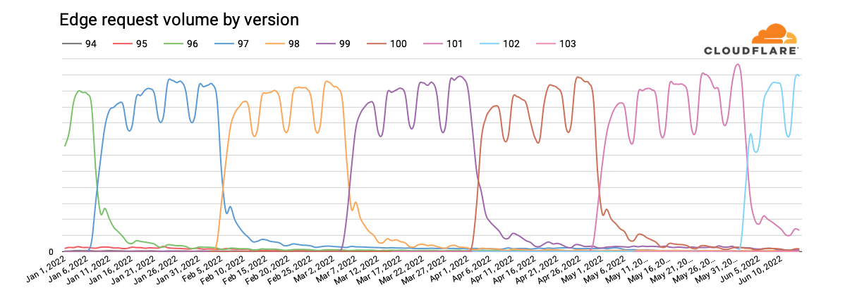
Looking at global request traffic to Cloudflare from Internet Explorer versions between January 1 and June 20, 2022, we see in the graph below that peak request volume for Internet Explorer 11 has declined by approximately one-third over that period. The clear weekly usage pattern suggests higher usage in the workplace than at home, and the nominal decline in traffic year-to-date suggests that businesses are not rushing to replace Internet Explorer with Microsoft Edge. However, we expect traffic from Internet Explorer 11 to drop more aggressively as Microsoft rolls out a two-phase plan to redirect users to Microsoft Edge, and then ultimately disable Internet Explorer. Having said that, we do not expect Internet Explorer 11 traffic to ever fully disappear for several reasons, including Microsoft Edge’s “IE Mode” representing itself as Internet Explorer 11, the ongoing usage of Internet Explorer 11 on Windows 8.1 and Windows 7 (which were out of scope for the retirement announcement), and automated (bot) traffic masquerading as Internet Explorer 11.
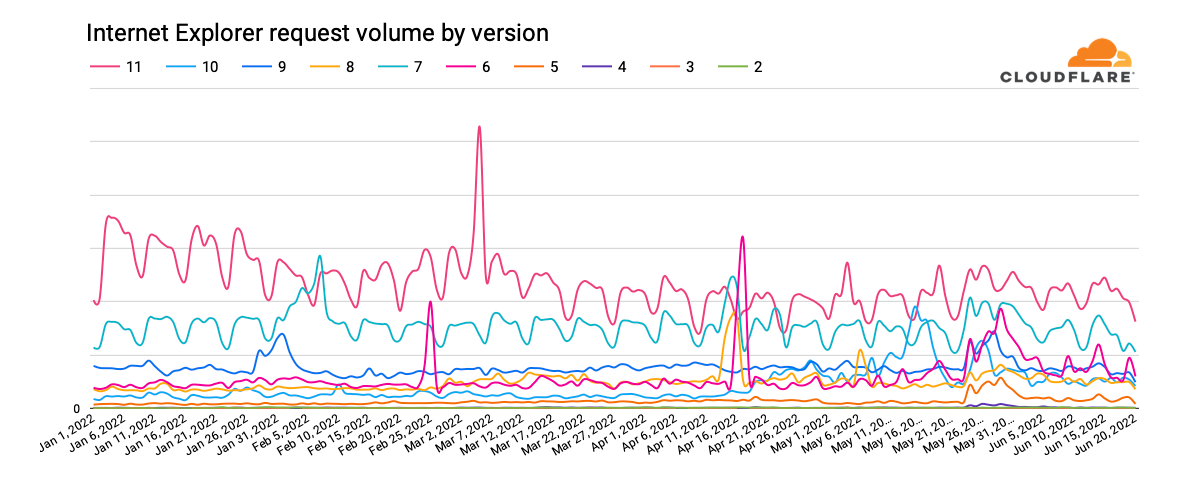
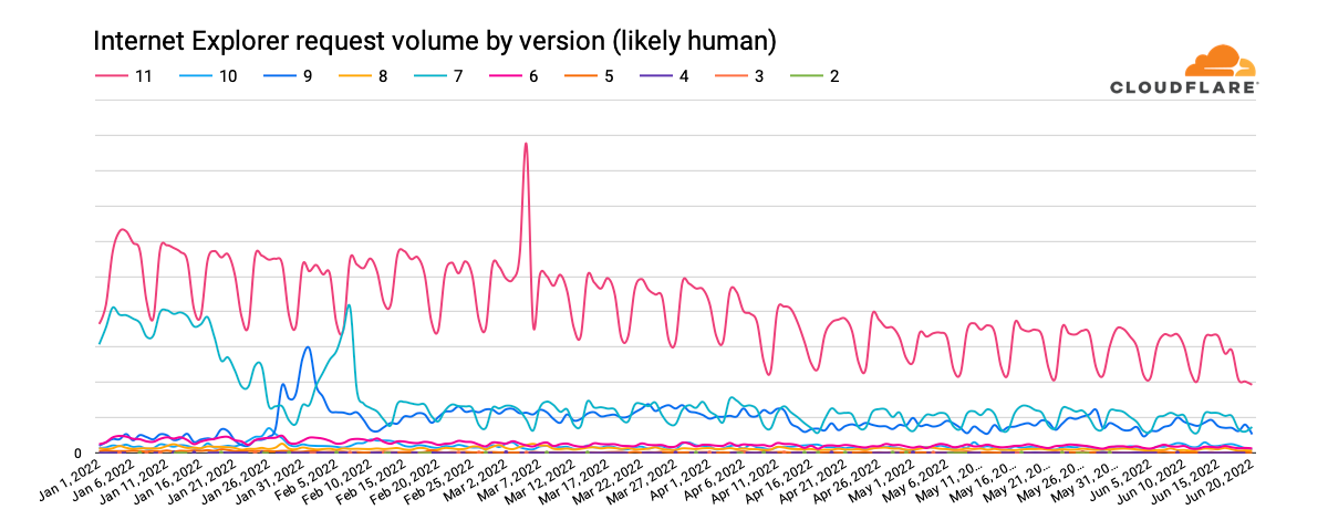
It is also apparent in the graph above that traffic from earlier versions of Internet Explorer has never fully disappeared. (In fact, we still see several million requests each day from clients purporting to be Internet Explorer 2, which was released in November 1995 — over a quarter-century ago.) After version 11, Internet Explorer 7, first released in October 2006 and last updated in May 2009, generates the next largest volume of requests. Traffic trends for this version have remained relatively consistent. Internet Explorer 9 was the next largest traffic generator through late May, when Internet Explorer 6 seemed to stage a comeback. (Internet Explorer 7 saw a slight bump in traffic at that time as well.)
Perhaps unsurprisingly, the United States has accounted for the largest volume of Internet Explorer 11 requests year-to-date. Similar to the global observation above, daily peak request traffic has declined by approximately one-third. With request volume approximately one-fourth that seen in the United States, Japan ostensibly has the next largest Internet Explorer 11 user base. (And published reports note that Internet Explorer’s retirement is likely to cause Japan headaches ‘for months’” because local businesses and government agencies didn’t take action in the months ahead of the event.)
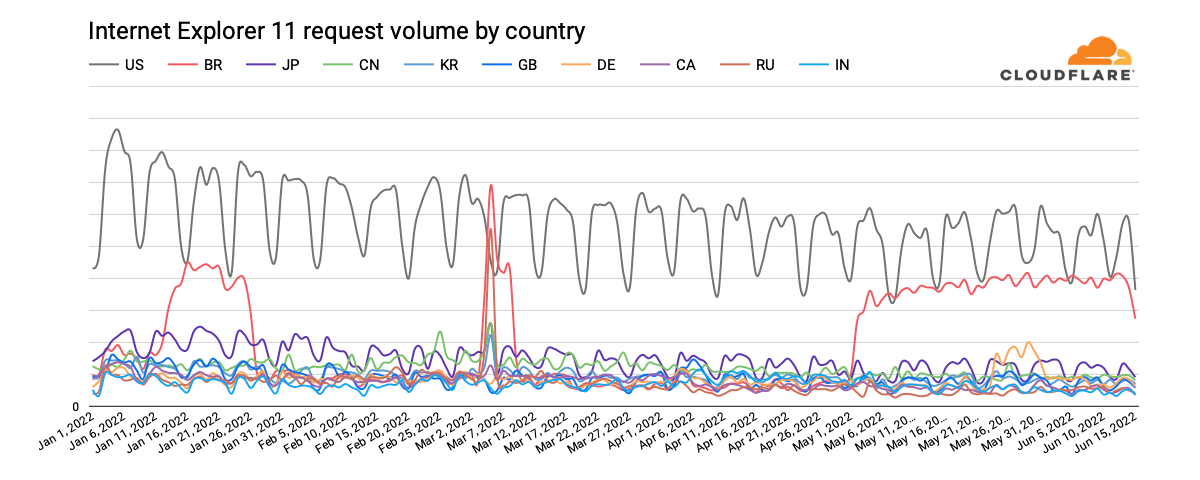
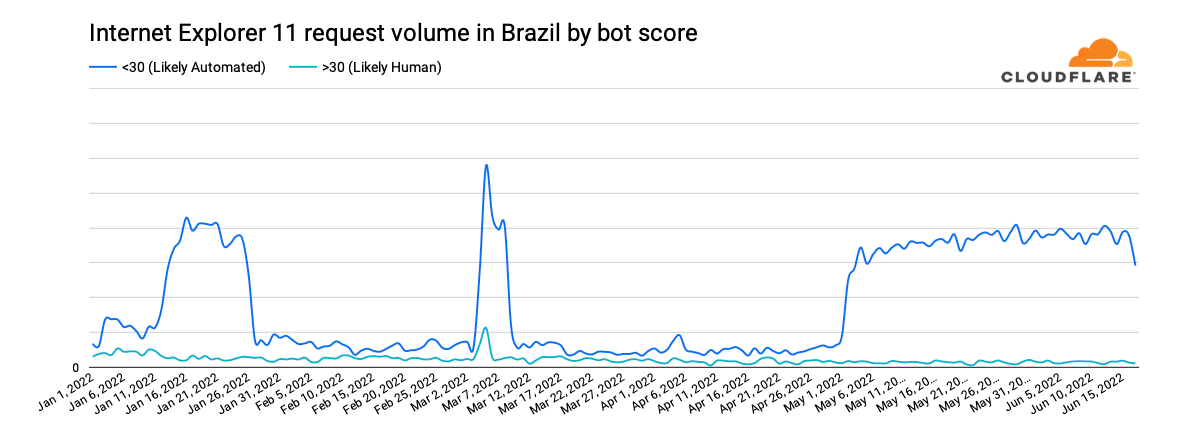
However, unusual shifts in Brazil’s request volume, seen in the graph above, are particularly surprising. For several weeks in January, Internet Explorer 11 traffic from the country appears to quadruple, with the same behavior seen from early May through mid-June, as well as a significant spike in March. Classifying the request traffic by bot score, as shown in the graph below, makes it clear that the observed increases are the result of automated (bot) traffic presenting itself as coming from Internet Explorer 11.
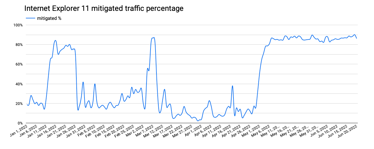
Further, analyzing this traffic to see what percentage of requests were mitigated by Cloudflare’s Web Application Firewall, we find that the times when the mitigation percentage increased, as shown in the graph below, align very closely with the periods where we observed the higher levels of automated (bot) traffic. This suggests that the spikes in Internet Explorer 11 traffic coming from Brazil that were seen over the last six months were from a botnet presenting itself as that version of the browser.
Building on the Brazil analysis, breaking out the traffic for each version by associated bot score can help us better understand the residual traffic from long-deprecated versions of Internet Explorer shown above. For requests with a bot score that characterizes the traffic as “likely human”, the graph below shows clear weekly traffic patterns for versions 11 and 7, suggesting that the traffic is primarily driven by systems primarily in use on weekdays, likely by business users. For Internet Explorer 7, that traffic pattern becomes more evident starting in mid-February, after a significant decline in associated request volume.
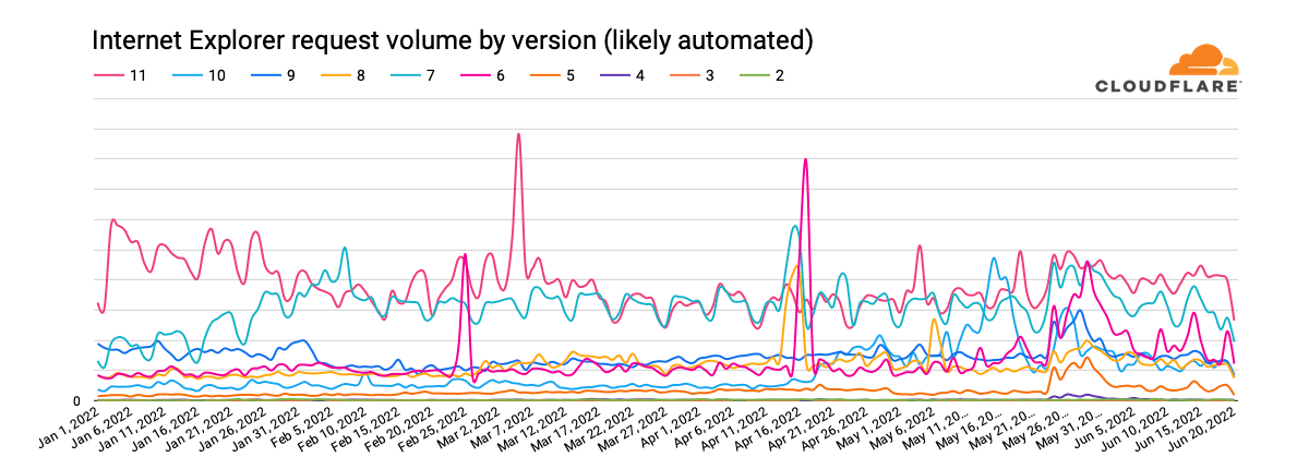
Interestingly, that decline in “likely human” Internet Explorer 7 request volume aligns with an increase in “likely automated” (bot) request volume for that version, visible in the graph below. Given that the “likely human” traffic didn’t appear to migrate to another version of Internet Explorer, the shift may be related to improvements to the machine learning model that powers bot detection that were rolled out in the January/February time frame. It is also interesting to note that “likely automated” request volume for both Internet Explorer 11 and 7 has been extremely similar since mid-March. It is not immediately clear why this is the case.
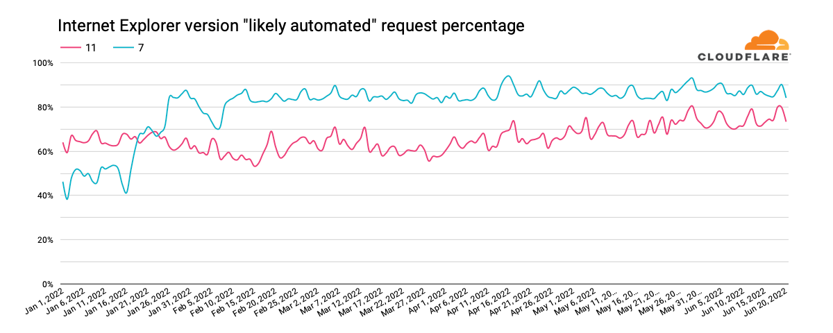
We can also use this data to understand what percentage of the traffic from a given version of Internet Explorer is likely to be automated (coming from bots). The graph below highlights the ratios for Internet Explorer 11 and 7. For version 11, we can see that the percentage has grown from around 60% at the start of 2022 to around 80% in June. For version 7, it starts the year in the 40% range, and more than doubles to over 80% in February and remains consistent at that level.
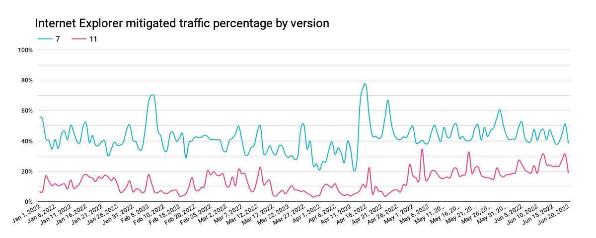
However, when we look at firewall mitigated traffic percentages, we don’t see the same clear alignment of trends as was visible for Brazil, as discussed above. In addition, only a fraction of the “likely automated” traffic was mitigated, suggesting that the automated traffic is split between being generated by bots and other non-malicious tools, such as performance testing.
Internet Explorer versions 6 & 9 were also discussed above, with respect to driving the largest volume of requests. However, when we examine the “likely automated” request ratios for these two browsers, we find that most of their traffic appears to be bot-driven. Internet Explorer 6 started 2022 at around 80%, growing to 95% in June. In contrast, Internet Explorer 9 starts the year around 90%, drops to 60% at the end of January, and then gradually increases back to the 75-80% range.
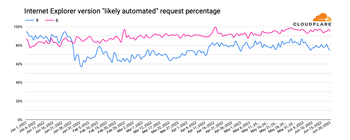
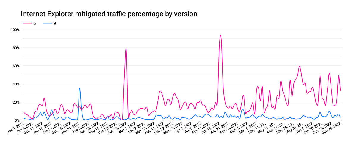
As Internet Explorer 6’s “likely automated” traffic has increased, the fraction of it that was mitigated has increased as well. The small bumps visible in the graph above align with the larger spikes in the graph below, potentially due to brief bursts of bot activity. In contrast, mitigated Internet Explorer 9 traffic has remained relatively consistent, even as its automated request percentage dropped and then gradually increased.
For the oldest, long-deprecated versions of Internet Explorer, automated traffic frequently comprises more than 80% of request volume, reaching 100% on multiple days year-to-date. Mitigated traffic generally amounted to under 30% of request volume, although Internet Explorer 2 frequently increased to the 50% range, spiking as high as 90%.
As Microsoft stated, “the future of Internet Explorer on Windows 10 is in Microsoft Edge.” Given that, we wanted to understand the usage patterns of Microsoft Edge. Similar to the analysis above, we looked at request volumes for the last ten versions of the browser year-to-date. The graph below clearly illustrates strong enterprise usage of edge, with weekday peaks, and lower traffic on the weekends. In addition, the four-week major release cycle cadence is clearly evident, with a long tail of usage extending across eight weeks due to enterprise customers who need an extended timeline to manage updates.
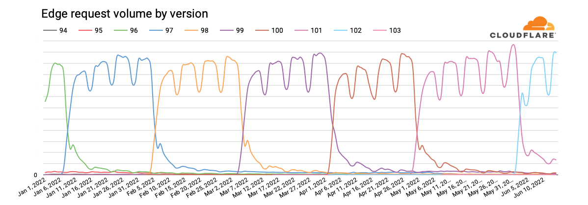
Having said that, in analyzing the split by bot score for these Edge versions, we note that only around 80% of requests are classified as “likely human” for about eight weeks after a given version is released, after which it gradually tapers to around 60%. The balance is classified as “likely automated”, suggesting that those who develop bots and other automated processes recognize the value in presenting their user agents as the latest version of Microsoft’s web browser. For Edge, there does not appear to be any meaningful correlation between firewall mitigated traffic percentages and “likely automated” traffic percentages or the traffic cycles visible in the graph above.
Analyzing traffic trends from deprecated versions of Internet Explorer brought to mind the “I’m not dead yet” scene from Monty Python and the Holy Grail with these older versions of the browser claiming to still be alive, at least from a traffic perspective. However, categorizing this traffic to better understand the associated bot/human split showed that the majority of Internet Explorer traffic seen by Cloudflare, including for Internet Explorer 11, is apparently not coming from actual browser clients installed on user systems, but rather from bots and other automated processes. For the automated traffic, analysis of firewall mitigation activity shows that the percentage likely coming from malicious bots varies by version.
As Microsoft executes its planned two-phase approach for actively moving users off of Internet Explorer, it will be interesting to see how both request volumes and bot/human splits for the browser change over time – check back later this year for an updated analysis.