Front: LLMs and Python bugs; scheduler regression; new Rust traits; dependency cooldowns; 7.1 merge window; Shor’s algorithm; drama at The Document Foundation.
This post was co-written with Ross Belmont, Senior Director, Rodrigo Duran, Strategist Director at Salesforce
Every minute counts when managing a critical infrastructure incident. Organizations need to quickly identify issues, diagnose root causes, and implement solutions—all while keeping customers informed. AWS DevOps Agent changes this by automating investigation and response, reducing mean time to resolution (MTTR) from hours to minutes.
In this post, you’ll learn how to integrate AWS DevOps Agent with Salesforce Hosted MCP Server to create an autonomous incident investigation workflow. This integration connects customer support cases directly to infrastructure diagnostics, reducing response times, and facilitating consistent incident resolution across your organization.
The Challenge: The Cost of Manual Incident Investigation
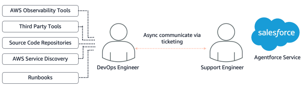
Customer complaints like “the website is slow” often trigger hours of investigation across distributed systems, fragmented telemetry, and multiple teams. Your customer support team lacks the deep infrastructure expertise to diagnose root causes, while your DevOps Engineers are constantly interrupted and pulled away from systematic improvements.
This handoff between teams creates friction:
Increased mean time to detect (MTTD) – Issues sit in queues waiting for the right expert
Extended mean time to resolve (MTTR) – Manual investigation across Amazon CloudWatch, AWS CloudTrail, application logs, and deployment history is time-consuming
Context loss – Information gets lost in translation between support tickets and infrastructure analysis
Reactive problem solving – Teams spend time on symptoms rather than preventing recurring issues
Figure 1 – Manual Support Process without DevOps Agent
AWS DevOps Agent integrated with Salesforce changes this paradigm by connecting support workflows directly to autonomous infrastructure investigation, eliminating manual handoffs and reducing investigation time.
How It Works – A Seamless Flow from Customer Complaint to Infrastructure Diagnosis
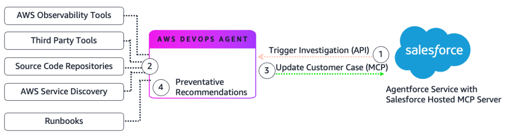
Figure 2 – Automated Support Process with DevOps Agent
Case Creation: Your customer reports an issue in Agentforce Service (e.g., “My Load Balancer is showing unavailable”). Salesforce Flow detects the new case and triggers the AWS DevOps Agent via an API or webhook call.
Autonomous Investigation: DevOps Agent starts an investigation and identifies the root cause. The agent queries AWS observability services, third-party platforms like Splunk and Datadog, code repositories, and CI/CD pipelines. It builds a dynamic topology graph to map relationships between application resources.
Case Enrichment: Investigation findings automatically post back to the Salesforce case, providing your support team with technical context and root cause analysis.
Preventative Recommendations: The agent suggests architectural improvements to help prevent recurrence.
Real-World Example: The Single Instance Outage
The Incident
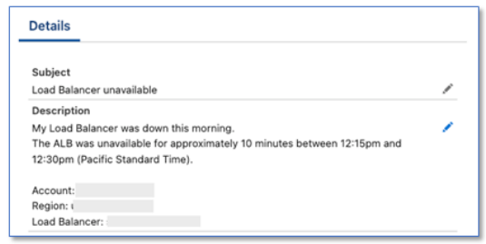
A customer opens a case in Agentforce Service reporting an application as unavailable.
Figure 3 – Agentforce Service case details
The Investigation
Salesforce Flow triggers DevOps Agent when the case is created:
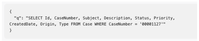
Case Retrieval: The agent uses the Salesforce soql_query tool to retrieve case details, including the customer’s account, incident description, and timing. The tool is made available via Salesforce Hosted MCP.
Figure 4 – Salesforce SOQL Query
Topology Discovery: The agent maps the infrastructure and identifies all components of the application.
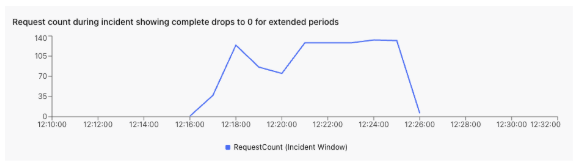
CloudWatch Metrics Analysis: The agent examines metrics during the incident window and discovers the count of requests dropped to zero during the unavailability period.
Figure 5 – Request Count Chart
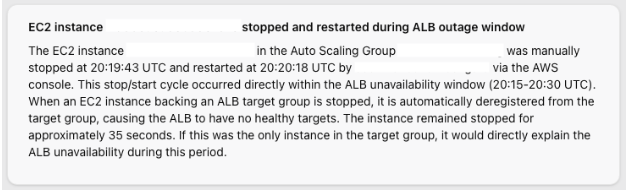
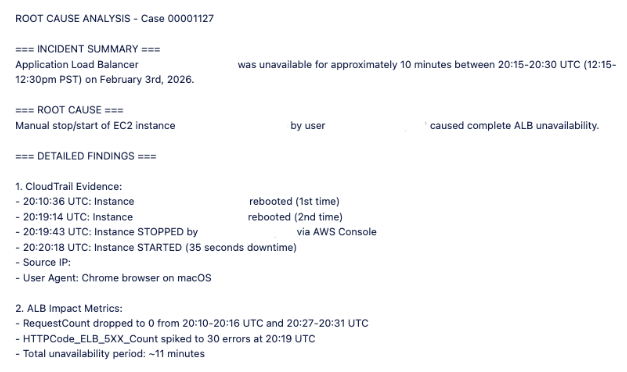
CloudTrail Event Analysis: The agent discovers a sequence of administrative actions that caused the downtime.
Figure 6 – CloudTrail Analysis
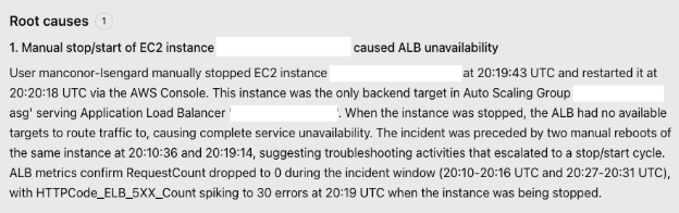
Root Cause Determination: The agent correlates the administrative actions with the metrics drop, identifying that an EC2 instance termination caused the outage.
Figure 7 – Root Cause Details
Case Update: The agent uses the Salesforce create_sobject_record tool to post findings to the case Activity feed. The tool is made available via Salesforce Hosted MCP.
The Result
Your Salesforce case now contains a comprehensive root cause analysis with timeline, affected resources, and contributing factors.
Figure 8 – Agentforce Service case updated with root cause
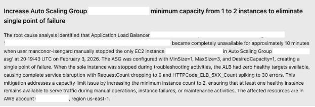
The Mitigation Plan
The agent generates an actionable mitigation plan showing how to prevent recurrence.
Figure 9 – Mitigation Plan
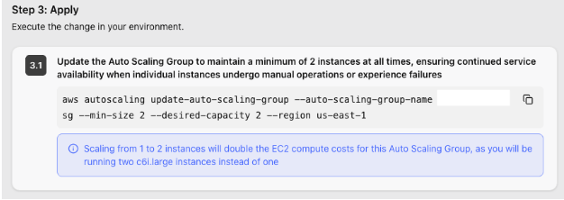
The agent also provides step-by-step remediation instructions that you can apply immediately. Due to length, this shows a portion of the plan.
Figure 10 – Step by Step Mitigation instructions
Technical Implementation
Prerequisites: Before implementing this integration, verify you have:
This integration requires configuration in both Salesforce and AWS. The following steps provide an overview of the setup process.
Create Agent Space: Set up a DevOps Agent Space in your AWS account with appropriate IAM roles and permissions.
Integrate Observability Tools: Connect your operational tools like Splunk, Datadog, or New Relic to provide the agent with telemetry data.
Connect Code Repositories: Link GitHub, GitLab, or AWS CodeCommit to enable the agent to correlate incidents with recent deployments.
Build Topology Mapping: Tag your infrastructure resources, so the agent focuses on components relevant to your application.
Add Skills: Configure the agent with instructions to direct the investigation – for example, to update Agentforce Service cases when investigations are complete.
Highlighted below are the key setup steps:
Create Agent Space
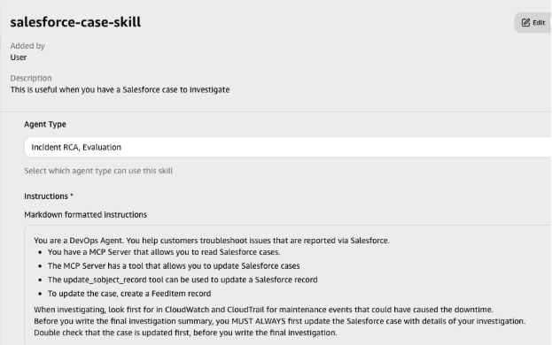
An Agent Space defines the AWS accounts, integrations, and access controls for your DevOps Agent investigations. When you create your Agent Space, configure a skill that instructs the agent to post investigation findings back to Salesforce cases.
Figure 11 – Agent Skill for Salesforce
The skill provides specific instructions for the agent’s workflow – in this case, directing it to update the originating Agentforce Service case when the investigation completes.
Salesforce Hosted MCP Server Setup
The Salesforce Hosted MCP Server enables AWS DevOps Agent to query case data and post investigation findings back to Salesforce. Configure the MCP Server in your Salesforce org using the following steps. For complete instructions, see the Salesforce documentation and the Salesforce Hosted MCP GitHub Repository.
Enable the Salesforce External MCP Service: Turn on the MCP functionality in your Salesforce org.
Create External Client App: Register the AWS DevOps Agent as an OAuth client in Salesforce with these settings:
Enable OAuth Settings with required scopes (see below)
Add the Salesforce Hosted MCP Server to Your Agent Space
In the AWS Console, register the Salesforce MCP Server with your Agent Space. This connection allows DevOps Agent to query Salesforce case data and post investigation findings.
After registration, test by manually triggering an investigation from the AWS Console. Instruct the agent to retrieve case details from Salesforce and post the root cause analysis back to the case.
In the next step, you’ll automate this workflow using Salesforce Flow, so investigations trigger automatically when cases are created.
Using Salesforce Flows
Salesforce Flows automate the connection between case creation and DevOps Agent investigations. Flow is a no-code automation tool that uses a visual drag-and-drop interface (Flow Builder) to automate business processes.
Configure a Flow trigger on your Case object to invoke DevOps Agent automatically when cases are created.
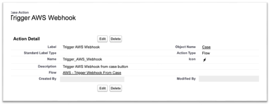
Figure 13 – Salesforce Trigger
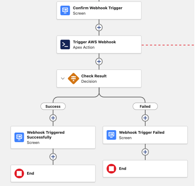
The Flow calls the DevOps Agent webhook with case details including the customer account, incident description, and timing. This triggers an autonomous investigation without requiring manual handoff to engineering teams. Due to length, this shows a portion of the Flow.
Figure 14 – Salesforce Flow
For implementation details and example code, see this Code repository
Connecting Salesforce Flow to AWS DevOps Agent
Configure how Salesforce Flow invokes the DevOps Agent webhook. Choose one of three integration approaches based on your requirements:
Option 1: External Service (Recommended for simplicity)External Service Integrate with AWS services using SigV4 (AWS Signature Version 4) authentication through Named Credentials. This no-code approach is the fastest way to establish the connection.
Option 2: Apex Class (Recommended for custom logic)Create an Apex class that your Flow calls to invoke the webhook. This approach provides flexibility to add custom business logic or error handling before triggering investigations.
Results and Impact
This integration transforms incident response by connecting customer support directly to autonomous infrastructure investigation:
Faster Incident Resolution: Autonomous investigation reduces mean time to resolution (MTTR) by eliminating manual log analysis. The agent detects and diagnoses issues immediately when cases are created, providing 24/7 coverage across time zones.
Reduced Manual Effort: SRE teams focus on systematic improvements instead of responding to individual incidents. Support teams receive technical insights without escalating to engineering, and every investigation follows the same thorough process.
Improved Customer Experience: Customers receive detailed root cause analysis within minutes of reporting an issue. This transparency builds trust, and the agent’s architectural recommendations help prevent recurring problems.
Organizational Learning: Every investigation is documented and searchable, creating a knowledge base of incident patterns. The agent identifies recurring issues across cases and suggests infrastructure improvements to address root causes.
Conclusion
Connecting AWS DevOps Agent with a Salesforce Hosted MCP Server creates an autonomous investigation workflow that eliminates manual handoffs between support and engineering teams. This integration reduces mean time to resolution through instant analysis, improves customer experience with rapid root cause updates, and enables proactive prevention through pattern recognition.
Building on our recent announcement of AWS Security Hub Extended —our full-stack enterprise security offering — we want to show you how we’re simplifying security procurement and operations for your multicloud environments. Whether you’re a security architect evaluating solutions or a CISO looking to streamline vendor management, this post walks through the streamlined experience that transforms how you acquire, deploy, and manage end-to-end enterprise security solutions across endpoint, identity, email, network, data, browser, cloud, AI, and security operations. Security Hub Extended brings together AWS security services with carefully curated security partners. Delivering better outcomes together through unified procurement, billing, and operations that significantly reduce vendor management overhead so you can focus on what matters most: protecting your organization.
The challenge we’re addressing
Security teams today spend too much time on vendor management, evaluating services, negotiating contracts, and managing multiple billing cycles instead of focusing on what matters most: managing risk. But the procurement challenge runs even deeper. Until now, customers really only had one option: sign multi-year agreements based solely on proof-of-concept testing and estimated annual usage. This forces organizations to commit budget before they can validate whether a solution will work for them at scale.
AWS Security Hub Extended transforms this procurement model. Security Hub Extended offers customers the option to get started with pay-as-you-go pricing and no commitments, so they can move fast and validate solutions in their actual environment. After they’ve confirmed a solution works at scale, they can then align their vendor strategy and sign longer-term commitments for even more favorable pricing.
Security Hub Extended provides a curated set of carefully chosen partner solutions with competitive pricing, unified billing through your AWS account, and seamless integration. Our initial launch partners, selected by customers for their proven value, include 7AI, Britive, CrowdStrike, Cyera, Island, Noma, Okta, Oligo, Opti, Proofpoint, SailPoint, Splunk, Upwind, and Zscaler.
Getting started with Security Hub Extended
AWS Security Hub consolidates threat analytics from Amazon GuardDuty, vulnerability management from Amazon Inspector, and sensitive data discovery from Amazon Macie, correlating these signals with Security Hub Exposure findings to determine overall risk, reachability, and assumability. Security Hub Extended builds on this foundation by adding curated partner solutions, extending these unified security operations across your entire organization including multicloud, on-premises, and endpoint environments. If you’re already using Security Hub, you can navigate directly to the Extended plan section.
Getting started with Security Hub is straightforward. From the AWS Management Console, search for Security Hub to start the onboarding walkthrough. If you’re not already a Security Hub customer, you can quickly complete onboarding by designating an AWS organization delegated administrator (DA) account. You can then centrally enable and manage Security Hub across your entire organization’s accounts and AWS Regions from a single location (see Introduction to AWS Security Hub). After you’ve onboarded, navigate to the Extended plan section to add curated partner solutions.
Figure 1: Security Hub centralized configuration
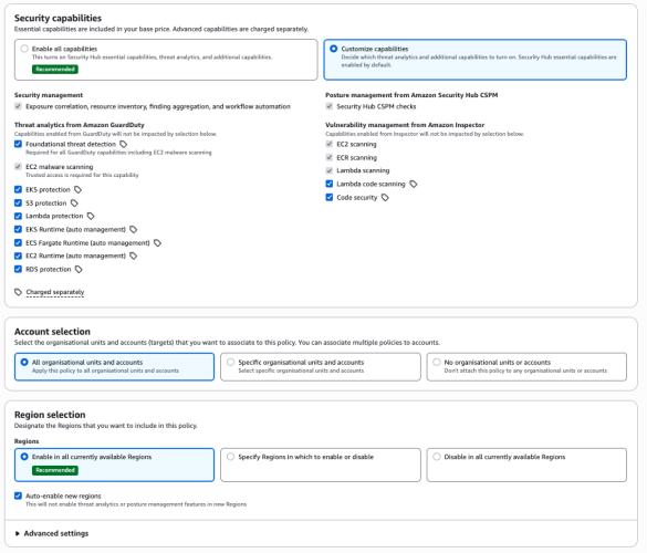
From this single interface, you can enable detection and response capabilities across your entire organization, provide granular configurations at the organizational unit or member account level, select specific Regions, and turn individual features on or off as needed.
Understanding risk through attack paths
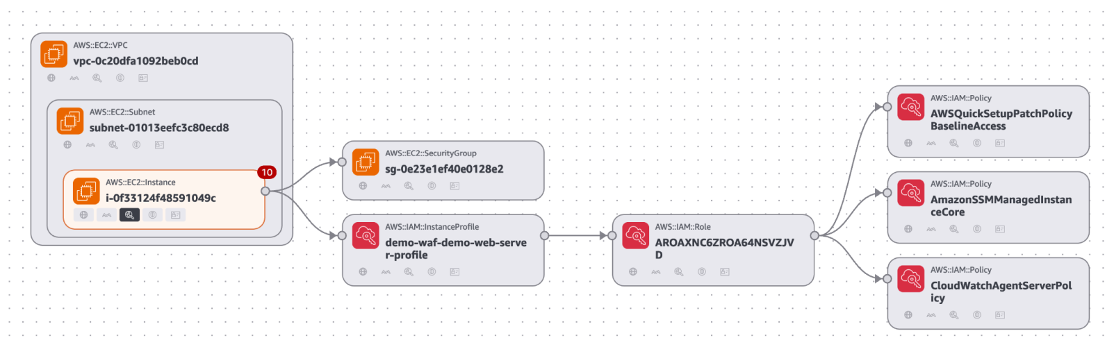
The Security Hub risk correlation engine identifies potential exposures by correlating threats, vulnerabilities, and misconfigurations to reveal how they connect and could lead to compromise of critical resources.
The attack path visualization in the preceding figure reveals critical insights including upstream root causes and blast radius, showing the potential impact if a threat actor exploits a vulnerability. You can use this visualization to focus on fixing the root cause rather than addressing symptoms. For example, updating one security group configuration can eliminate the entire attack path, cutting off all downstream exposure.
Accessing Security Hub Extended
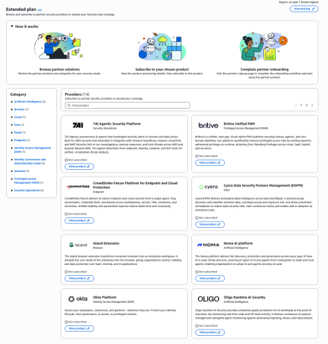
You can find Security Hub Extended, shown in the following figure, in the left navigation pane under Management in your Security Hub delegated administrator (DA) account; Security Hub Extended will only be visible from the delegated administrator account. The Extended plan brings curated third-party security solutions directly into the Security Hub experience. Because Extended is built into Security Hub, there’s no separate console to manage. You discover, subscribe to, and operate curated partner solutions from the same place you manage enterprise security, delivering unified operations across your entire security estate.
Transparent, competitive pricing consolidated with Security Hub
Unlike traditional third-party engagements that require lengthy negotiations, private pricing deals, and multi-year commitments, Security Hub Extended offers complete pricing transparency. Every partner solution displays clear, competitive monthly pay-as-you-go rates billed directly with Security Hub requiring no commitments. For example, Cloud Security from Upwind costs $3.75 per resource per month, and Identity Security from Okta costs $20 per user per month.
All Security Hub Extended offerings are also eligible for AWS Enterprise Discount Program (EDP) discounts that will be applied automatically. If you have an existing AWS enterprise discount agreement, those discounts automatically apply to Security Hub Extended offerings, further reducing your effective costs. All partner solutions you deploy through Security Hub Extended appear on your consolidated AWS bill, no separate invoices or payment processes.
Streamlined onboarding
Adopting curated partner solutions through Security Hub Extended is straightforward. Choose View Product to initiate an automated workflow. Depending on the solution, you’ll either be directed to the partner onboarding console or provide information for the partner to guide you through their onboarding process tailored to your environment.
Billing begins only after you’re fully activated on the partner solution and starts automatically, no additional action is required to benefit from the unified billing. If you’re already using one of the curated partner solutions, transitioning to Security Hub Extended for consolidated billing and flexible pricing won’t disrupt your current services. Now, instead of receiving separate invoices for each partner in addition to Amazon Inspector, GuardDuty, and Security Hub CSPM you get one unified bill through Security Hub. This consolidates visibility to support better understanding of spend and to manage cost.
Unified operations
Security Hub Extended unifies security operations by consolidating findings from AWS and curated partner solutions. All findings use the Open Cybersecurity Schema Framework (OCSF) for consistency, without the need for complex data normalization, transformation, and extract, transform, and load (ETL) processes.
When you deploy solutions such as CrowdStrike, Noma, and Upwind alongside Splunk and 7AI through Security Hub Extended, security findings automatically flow into Security Hub and then seamlessly route to Splunk and 7AI. All in OCSF format so your security team can focus on responding to threats, not managing pipelines, so you can quickly identify and respond to security risks that span boundaries—from endpoint compromises to cloud infrastructure—without spending valuable time on manual integration work.
The full-stack security vision
Security Hub Extended represents a shift in how you discover, procure, and build comprehensive security programs. Instead of managing dozens of vendor relationships, negotiating separate contracts, agreeing to multi-year annual commitments, and integrating disparate tools, you now have one procurement process through AWS, one bill with transparent competitive pay-as-you-go pricing, one console for unified security operations, one support channel for AWS Enterprise Support customers, and one schema (OCSF) for all security findings. The result: reduced security risk, improved team productivity, and a more unified approach to security operations across your enterprise.
Get started
Try Security Hub Extended today and experience how simplified procurement and unified operations can transform your security program. Security Hub Extended is generally available globally in all AWS commercial Regions where Security Hub is available. We’ve also published a walk through video to further explain how Security Hub Extended works.
It’s still Day 1, but we’re iterating fast, so share your feedback with us on AWS re:Post for Security Hub or through your AWS Support contacts and watch for future blog posts on our progress.
Data strategy can use geospatial data to provide organizations with insights for decision-making and operational optimization. By incorporating geospatial data (such as GPS coordinates, points, polygons and geographic boundaries), businesses can uncover patterns, trends, and relationships that might otherwise remain hidden across multiple industries, from aviation and transportation to environmental studies and urban planning. Processing and analyzing this geospatial data at scale can be challenging, especially when dealing with billions of daily observations.
In this post, we explore how to use Apache Sedona with AWS Glue to process and analyze massive geospatial datasets.
Introduction to geospatial data
Geospatial data is information that has a geographic component. It describes objects, events, or phenomena along with their location on the Earth’s surface. This data includes coordinates (latitude and longitude), shapes (points, lines, polygons), and associated attributes (such as the name of a city or the type of road).
Key types of geospatial geometries (and examples of each in parentheses) include:
Point – Represents a single coordinate (a weather station).
MultiPoint – A collection of points (bus stops in a city).
LineString – A series of points connected in a line (a river or a flight path).
MultiPolygon – Multiple polygons (national parks in a country).
Geospatial datasets come in different formats, each designed to store and represent different types of geographic information. Common formats for geospatial data are vector formats (Shapefile, GeoJSON), raster formats (GeoTIFF, ESRI Grid), GPS formats (GPX, NMEA), web formats (WMS, GeoRSS) among others.
Core concepts of Apache Sedona
Apache Sedona is an open-source computing framework for processing large-scale geospatial data. Built on top of Apache Spark, Sedona extends Spark’s capabilities to handle spatial operations efficiently. At its core, Sedona introduces several key concepts that enable distributed spatial processing. These include Spatial Resilient Distributed Datasets (SRDDs), which allow for the distribution of spatial data across a cluster, and Spatial SQL, which provides a familiar SQL-like interface for spatial queries. Some of the core capabilities of Apache Sedona are:
Efficient spatial data types like points, lines and polygons.
Spatial operations and functions such as ST_Contains (check if point is inside of a polygon), ST_Intersects (check if point is inside of a polygon), ST_H3CellIDs (geospatial indexing system developed by Uber, return the H3 cell ID(s) that contain the given point at the specified resolution).
Spatial joins to combine different spatial datasets.
Integration with Spark SQL (geospatial functions to run spatial SQL queries).
Spatial indexing techniques, such as quad-trees and R-trees, to optimize query performance.
For more information about the functions available in Apache Sedona, visit the official Sedona Functions documentation.
Use case
This use case consists of a global air traffic visualization and analysis platform that processes and displays real-time or historical aircraft tracking data on an interactive world map. Using unique aircraft identifiers from the International Civic Aviation Organization (ICAO), the system ingests trajectory records containing information such as geographic position (latitude and longitude), altitude, speed, and flight direction, then transforms this raw data into two complementary visual layers. The Flight Tracks Layer plots the routes traveled by each aircraft individually, allowing for the analysis of specific trajectories and navigation patterns. The Flight Density Layer uses hexagonal spatial indexing (H3) to aggregate and identify regions of higher air traffic concentration worldwide, revealing busy air corridors, aviation hubs, and high-density flight zones.
The dataset used for this use case is historical flight tracker data from ADSB.lol. ADSB.lol provides unfiltered flight tracker with a focus on open data. Data is also freely available via the API. The data contains a file per aircraft, a JSON gzip file containing the data for that aircraft for the day.
This is a JSON trace file format sample:
{
    icao: "0123ac", // hex id of the aircraft
    timestamp: 1609275898.495, // unix timestamp in seconds since epoch (1970)
    trace: [
        [ seconds after timestamp,
            lat,
            lon,
            altitude in ft or "ground" or null,
            ground speed in knots or null,
            track in degrees or null, (if altitude == "ground", this will be true heading instead of track)
            flags as a bitfield: (use bitwise and to extract data)
                (flags & 1 > 0): position is stale (no position received for 20 seconds before this one)
                (flags & 2 > 0): start of a new leg (tries to detect a separation point between landing and takeoff that separates flights)
                (flags & 4 > 0): vertical rate is geometric and not barometric
                (flags & 8 > 0): altitude is geometric and not barometric
             ,
            vertical rate in fpm or null,
            aircraft object with extra details or null,
            type / source of this position or null,
            geometric altitude or null,
            geometric vertical rate or null,
            indicated airspeed or null,
            roll angle or null
        ],
    ]
}
For this use case, this is a simplified schema of the dataset after processing:
icao - Unique aircraft identifier
timestamp - Epoch timestamp of the observation (converted to readable format)
trace.lat / trace.lon - Latitude and longitude of the aircraft
trace.altitude - Aircraft altitude
trace.ground_speed - Ground speed
geometry - Geospatial geometry of the observation point (Point)
Solution overview
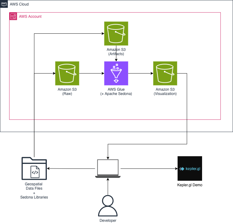
This solution enables aircraft tracking and analysis. The data can be visualized on maps and used for aviation management and safety applications. The process begins with data acquisition, extracting the compressed JSON files from TAR archives, then transforms this raw data into geospatial objects, aggregating them into H3 cells for efficient analysis. The processed data schema includes ICAO aircraft identifiers, timestamps, latitude/longitude coordinates, and derived fields such as H3 cell identifiers and point counts per cell. This structure allows detailed tracking of individual flights and aggregate analysis of traffic patterns. For visualization, you can generate density maps using the H3 grid system and create visual representations of individual flight tracks. The architecture data flow is as follows:
Data ingestion – Aircraft observation data stored as JSON compressed files in Amazon Simple Storage Service (Amazon S3).
Data processing – AWS Glue jobs using Apache Sedona for geospatial processing.
Data visualization – Spark SQL with Sedona’s spatial functions to extract insights and export data to visualize the information in a map on Kepler.gl.
The following figure illustrates this solution.
Prerequisites
You will need the following for this solution:
An AWS Account and a user with AWS Console access.
An IAM role for AWS Glue with list, read, and write permissions for Amazon S3 buckets.
An Amazon S3 Bucket for flight files. For this example, name the bucket blog-sedona-nessie-<account_number>-<aws_region>, using your account number and region.
An Amazon S3 bucket for artifacts and Sedona libraries. For this example, name the bucket blog-sedona-artifacts-<account_number>-<aws_region>, using your account number and region.
Download the AWS Glue script from AWS Sample to process the geospatial data.
Review the AWS Glue security best practices, especially IAM least-privilege, encryption for sensitive data at rest and in transit, and configuring VPC Endpoints to prevent data from routing through the public internet.
Solution walkthrough
From now on, executing the next steps will incur costs on AWS. This step-by-step walkthrough demonstrates an approach to processing and analyzing large-scale geospatial flight data using Apache Sedona and Uber’s H3 spatial indexing system, using AWS Glue for distributed processing and Apache Sedona for efficient geospatial computations. It explains how to ingest raw flight data, transform it using Sedona’s geospatial functions, and index it with H3 for optimized spatial queries. Finally, it also demonstrates how to visualize the data using Kepler.gl. For data processing, it is possible to use both Glue scripts and Glue notebooks. In this post, we will focus only on Glue scripts.
Upload the Apache Sedona libraries to Amazon S3
Open your OS terminal command line.
Create a folder to download the Sedona libraries and name it jar.
	# Create a directory for the Sedona libraries (JARs files)
	mkdir jar
	# Go to the folder JARs folder
	cd jar
	# Download the geospatial flight files in the folder created
	wget https://github.com/adsblol/globe_history_2025/releases/download/v2025.05.29-planes-readsb-prod-0tmp/v2025.05.29-planes-readsb-prod-0tmp.tar.aa
	wget https://github.com/adsblol/globe_history_2025/releases/download/v2025.05.29-planes-readsb-prod-0tmp/v2025.05.29-planes-readsb-prod-0tmp.tar.ab
Extract the flight files.
	# Combine the two the tar files together
	cat v2025.05.29* >> combined.tar
	# Extract the json flight files from the tar file
	tar xf combined.tar
Copy the flight files to Amazon S3. In this case, we are using the S3 folder: s3://blog-sedona-nessie-<account_number>-<aws_region>/raw/adsb-2025-05-28/traces/.
	# Copy the json flight files to Amazon S3
	aws s3 cp ./traces/ s3://blog-sedona-nessie-<account_number>-<aws_region>/raw/adsb-2025-05-28/traces/ --recursive
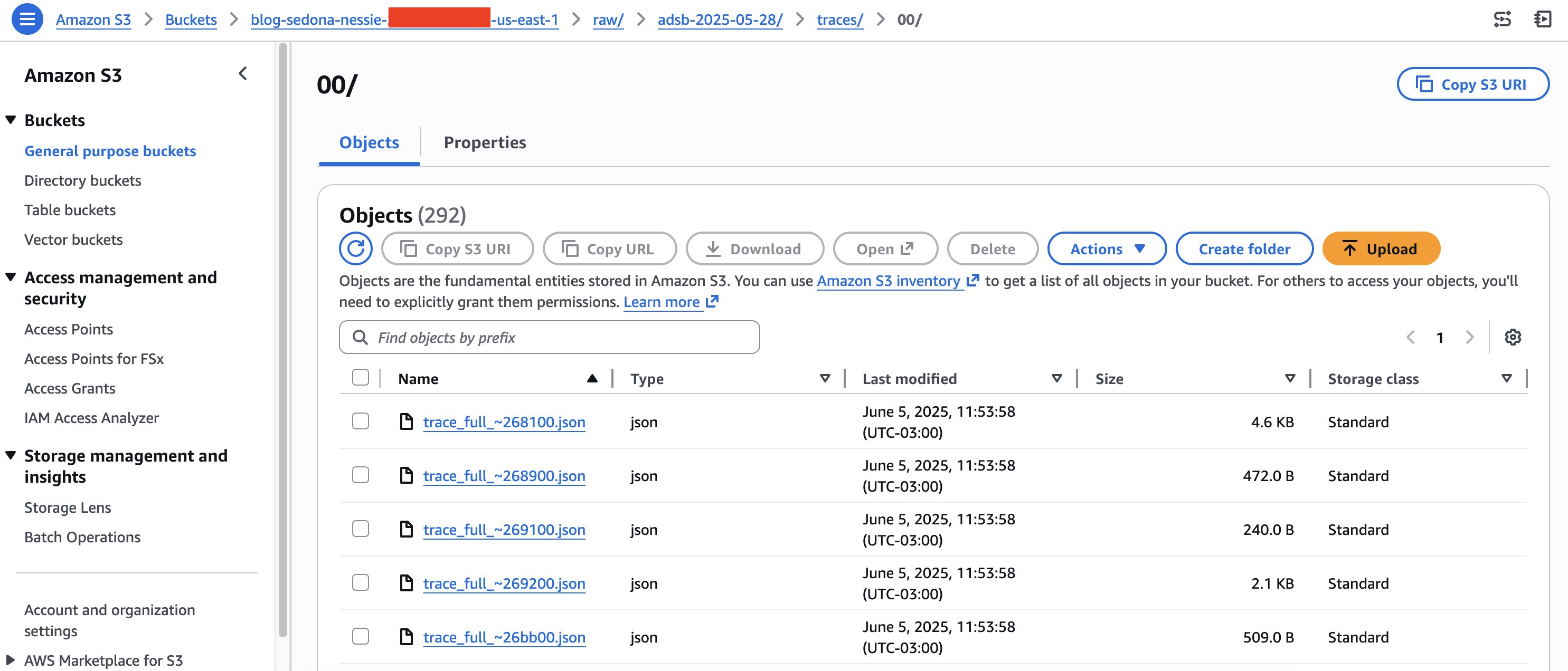
Your Amazon S3 folder should now look similar to the following image.
Create an AWS Glue job and set up the job
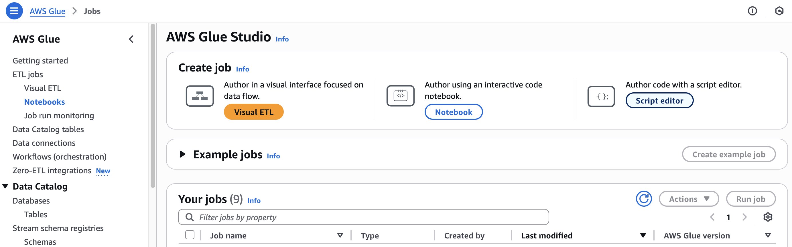
Now, we are ready to define the AWS Glue job using Apache Sedona to read the geospatial data files. To create a Glue job:
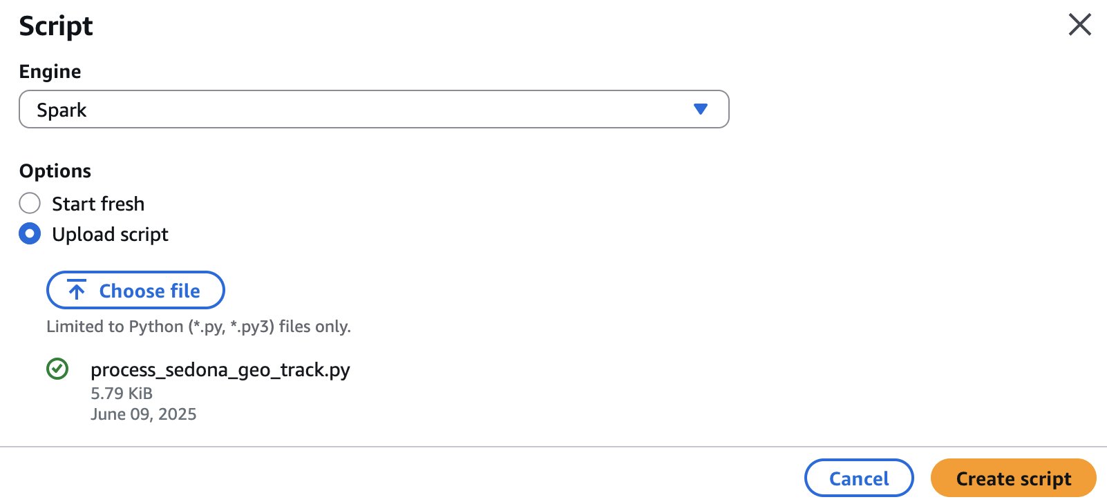
On the Script screen, for the engine, choose Spark, then select the option Upload script.
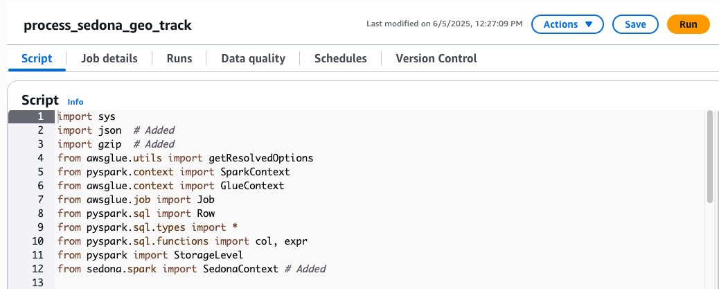
Choose Choose file. Find the process_sedona_geo_track.py file, then choose Create script.
Rename the job from Untitled to process_sedona_geo_track.
Choose Save.
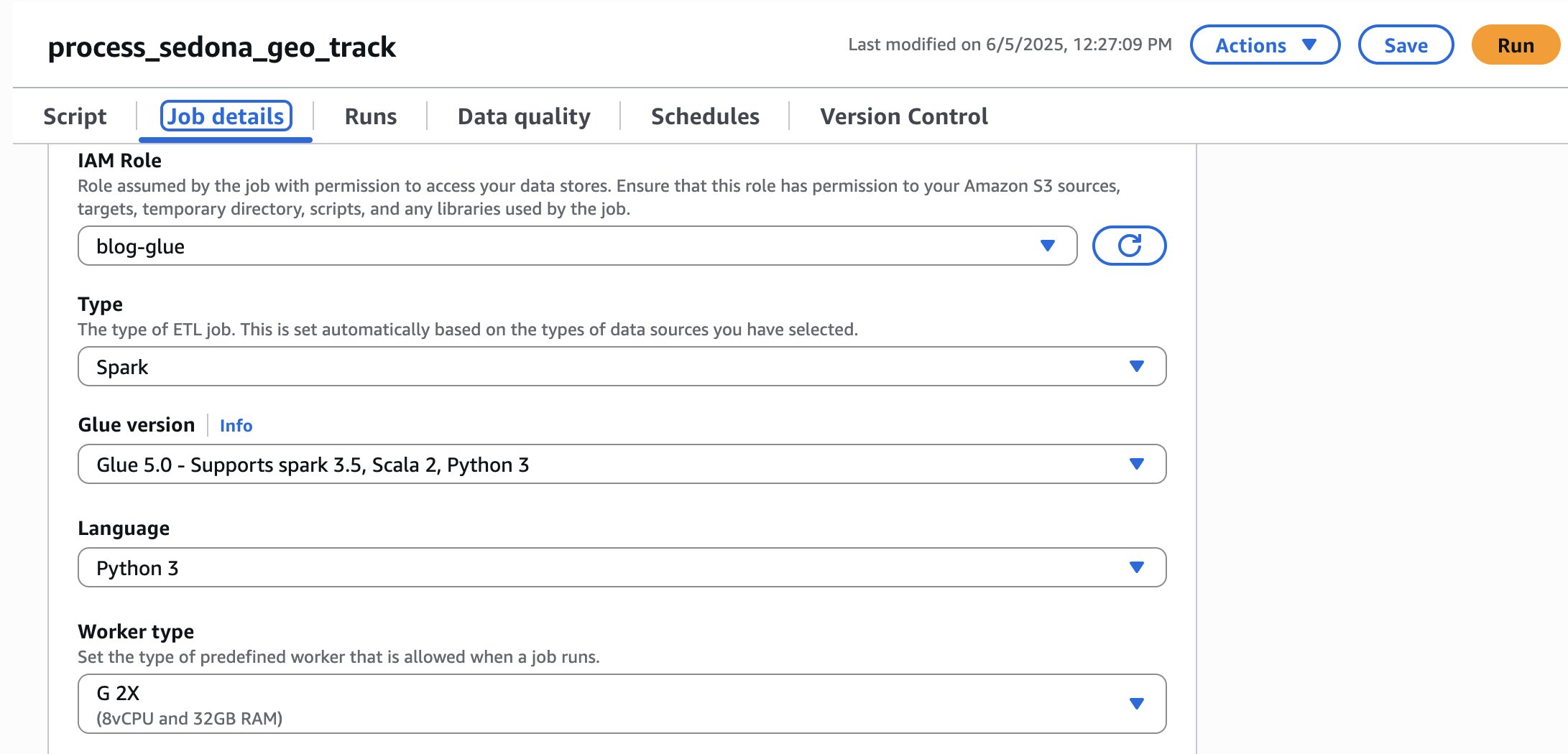
Now, let’s set up the AWS Glue job. Choose Job Details.
Choose the IAM Role created to be used with Glue. For this example, we use blog-glue.
Set the Glue version to Glue 5.0 and the Worker type as needed. For this example, G.1X is sufficient, but we use G.2X to speed up processing.
Now, let’s import the libraries for Apache Sedona.
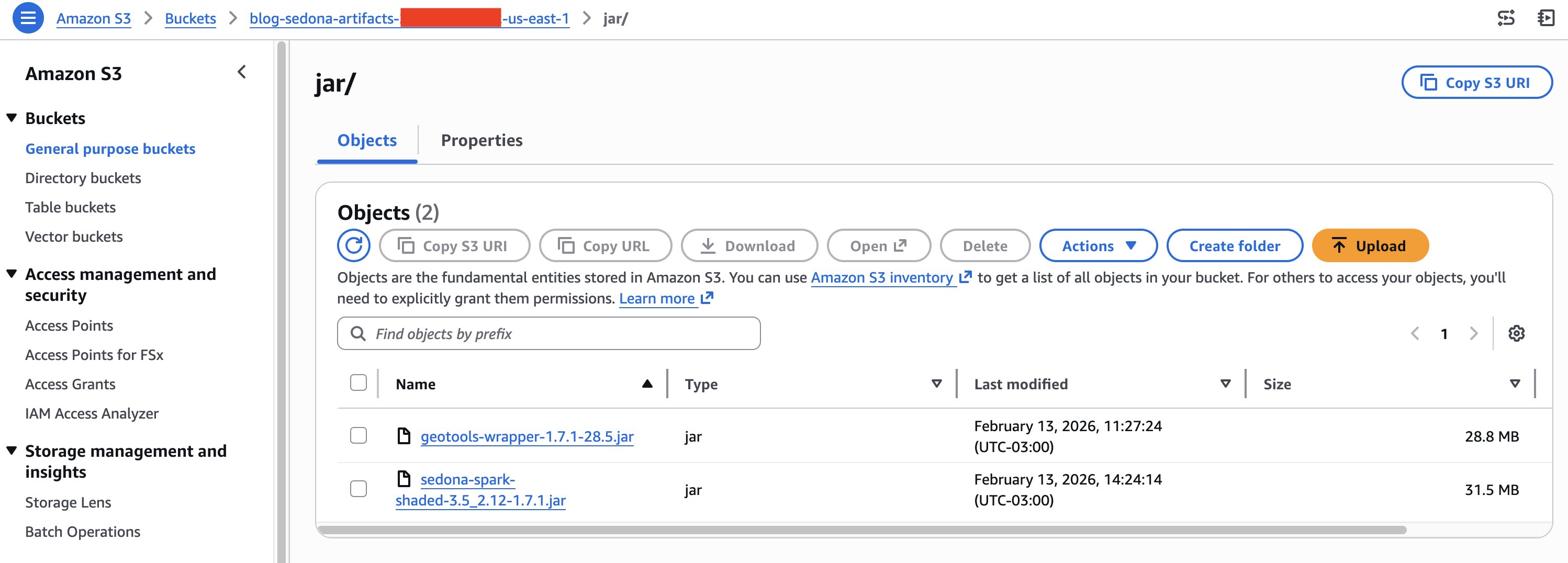
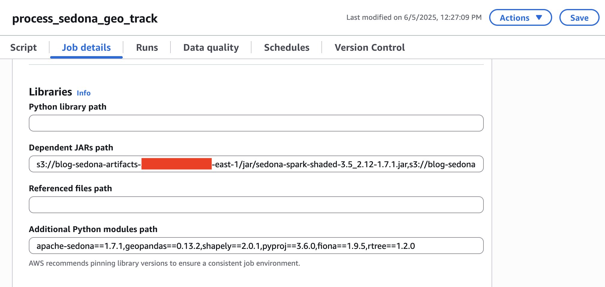
In the Dependent JARs path, type the path of the JAR files for Apache Sedona that you uploaded in the preceding steps. For this example, we used s3://blog-sedona-artifacts-<account_number>-<aws_region>/jar/sedona-spark-shaded-3.5_2.12-1.7.1.jar,s3://blog-sedona-artifacts-<account_number>-<aws_region>/jar/geotools-wrapper-1.7.1-28.5.jar
In Additional Python modules path, enter the modules for Apache Sedona: apache-sedona==1.7.1,geopandas==0.13.2,shapely==2.0.1,pyproj==3.6.0,fiona==1.9.5,rtree==1.2.0
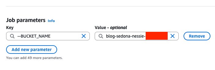
In the Job parameters section, in the Key field, type —BUCKET_NAME. For its Value, enter your bucket name. In this example, ours is blog-sedona-nessie-<account_number>-<aws_region>.
Choose Save.
Processing the geospatial flights data
Before we run the job, let’s understand how the code works. First, import the Apache Sedona libraries:
import json
import gzip
from sedona.spark import SedonaContext
Next, initialize the Sedona context using an existing Spark session:
sedona = SedonaContext.create(spark)
After that, create a function for handling compressed JSON data:
def parse_gzip_json(byte_content):
        try:
            decompressed = gzip.decompress(byte_content)
            return json.loads(decompressed.decode('utf-8'))
        except Exception as e:
            print(f"Error during gzip parse: {str(e)}")
            return None
Add a function to transform raw tracking data into a structured format suitable for a valid coordinates process:
def flatten_records(json_obj):
    records = []
    if "trace" in json_obj and isinstance(json_obj["trace"], list):
        for point in json_obj["trace"]:
            if len(point) >= 3:
                lat, lon = float(point[1]), float(point[2])
                if -90 <= lat <= 90 and -180 <= lon <= 180:
                    records.append(Row(
                        icao=json_obj.get("icao", None),
                        timestamp=json_obj.get("timestamp", None),
                        lat=lat,
                        lon=lon
                    ))
    return records
The flat_rdd variable applies these functions to the structured data from the original gzipped JSON. Each element in this RDD is a Row object representing a single data point from an aircraft’s trace, with fields for ICAO, timestamp, latitude, and longitude.
flat_rdd = raw_rdd.map(lambda x: parse_gzip_json(x[1])).filter(lambda x: x is not None).flatMap(flatten_records)
The ADSB trace files contain a deeply nested JSON structure where the trace field holds an array of mixed-type arrays, compressed in Gzip format. For this specific case, developing a UDF represented one of the most practical and efficient solutions. Since Gzip is a non-splittable format, Spark is unable to parallelize processing, constraining both methods to a single worker per file and processing the data multiple times across JVM decompression, full JSON parsing, and subsequent re-parsing operations. The UDF bypasses all of this by reading raw bytes and doing everything in a single Python pass: decompress → parse → extract → validate, returning only the small set of needed fields directly to Spark.
The Spark SQL query processes geographic trace data using the H3 hexagonal grid system, converting point data into a regularized hexagonal grid that can help identify areas of high point density. A resolution of 5 was adopted, producing hexagons of approximately 253 km² (roughly the same size as the city of Edinburgh, Scotland, which is approximately 264 km²), for its ability to effectively capture route density patterns at the city and metropolitan level.
h3_traces_df = spark.sql("""
WITH base_h3 AS (
    SELECT
        ST_H3CellIDs(geometry, 5, false)[0] AS h3_index,
        lat,
        lon
    FROM traces
)
SELECT
    COUNT(*) AS num, -- Count points in each H3 cell
    h3_index,
    AVG(lon) AS center_lon,
    AVG(lat) AS center_lat
FROM base_h3
GROUP BY h3_index
""")
Finally, this code prepares the datasets for visualization purposes. The first dataset is based on the aircraft unique identifier. The complete dataset for a single day can contain more than 80 million data points. A random sampling rate of 0.1% was applied, which proves sufficient to illustrate route density patterns without overwhelming the Kepler.gl browser renderer. The second dataset aggregates trace points into hexagonal spatial cells (result from the query above).
On the ETL jobs >> Notebooks page, choose the job name process_sedona_geo_track.
Choose Run.
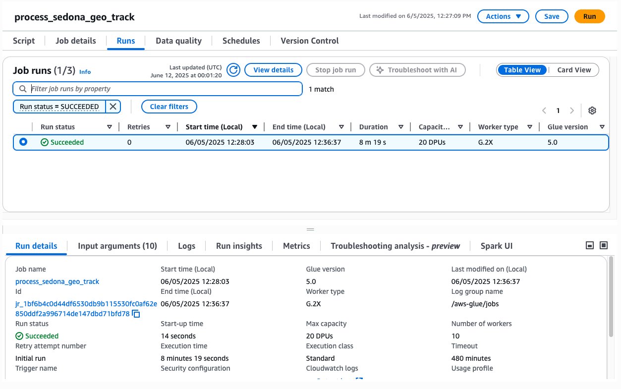
Now, it is possible to monitor the job by choosing the Runs tab.
It may take a few minutes to run the entire job. It took nearly 8 minutes to process approximately 2.50 GB (67,540 compressed files) with 20 DPUs. After the job is processed, you should see your job with the status Succeeded.
Now your data should be saved for a preview visualization demo in a folder named s3://blog-sedona-nessie-<account_number>-<aws_region>/visualization/.
Performance insights
The workload characterization of this job reveals a CPU-intensive profile, primarily because of the processing of small binary files with GZIP compression and subsequent JSON parsing. Given the inherent nature of this pipeline, which includes Python UDF serialization and partial single-partition write stages, linear scaling does not yield proportional performance gains. The following table presents an analysis of AWS Glue configurations, evaluating the trade-off between computational capacity, execution duration, and associated costs:
Duration
Capacity (DPUs)
Worker type
Glue version
Estimated Cost*
10 m 7 s
32 DPUs
G.1X
5
$2.34
11 m 50 s
10 DPUs
G.1X
5
$0.88
19 m 7 s
4 DPUs
G.1X
5
$0.59
8 m 19 s
20 DPUs
G.2X
5
$1.32
*Estimated Cost = DPUs x Duration (hours) x $0.44 per DPU-hour (us-east-1)
Visualizing and analyzing geospatial data with Kepler.gl
Kepler.gl is an open-source geospatial analysis tool developed by Uber with code available at Github. Kepler.gl is designed for large-scale data exploration and visualization, offering multiple map layers, including point, arc, heatmap, and 3D hexagon. It supports various file formats like CSV, GeoJSON, and KML. In this use case, we will use Kepler.gl to present interactive visualizations that illustrate flight patterns, routes, and densities across global airspace.
Downloading the geospatial files
Before we can view the graph, we will need to download the flight files to our local machine, unzip them, and rename them (to make it easier to identify the files).
Open your OS terminal command line.
Create the folders to download the data processed in the steps before. In this case, we create kepler and kepler_csv.
	#create kepler folders: first folder is to download the files,
	#second folder is to organize the files to use in the next step
	mkdir kepler
	mkdir kepler_csv
Replace the bracketed variables with your account and directory information, then download all the CSV files.
	#copy the files from Amazon S3 to local machine
	aws s3 cp s3://blog-sedona-nessie-<account_number>-<aws_region>/visualization/ /<user_directory>/kepler --recursive
Extract the files, rename them, and move them to another folder.
	# Extract the files processed by Spark and Sedona
	gzip -d ./kepler/kepler_h3_density/*.gz
	gzip -d ./kepler/kepler_track_points_sample/*.gz

	# Rename the Spark output files to more readable names
	cd ./kepler/kepler_h3_density/
	ls
	mv part-00000-*.csv kepler_h3_density.csv
	cd ..

	cd ./kepler/kepler_track_points_sample/
	ls
	mv part-00000-*.csv kepler_track_points_sample.csv
	cd ..

	# Ensure the output folder exists
	mkdir -p ../kepler_csv

	# Copy the renamed CSV files to the folder that will be used as input in kepler.gl
	cp ./kepler/kepler_h3_density/*.csv ../kepler_csv
	cp ./kepler/kepler_track_points_sample/*.csv ../kepler_csv
Your kepler_csv folder should look similar to the return of the command below.
	#list the files in the kepler_csv directory
	ls -l
	total 11684
	-rw-rw-r-- 1 ec2-user ec2-user 8630110 Jun 12 14:47 kepler_h3_density.csv
	-rw-rw-r-- 1 ec2-user ec2-user 3331763 Jun 12 14:47 kepler_track_points_sample.csv
Visualizing the data in a graph
Now that you have saved the data to your local machine, you can analyze the flight data through interactive map graphics. To import the data into the Kepler.gl web visualization tool:
Drag and drop both CSV files (flight_points and h3_density) into the upload area.
Confirm that both datasets are loaded successfully.
Delete all layers.
Create the Flight Density Layer:
Choose Add Layer in the left panel.
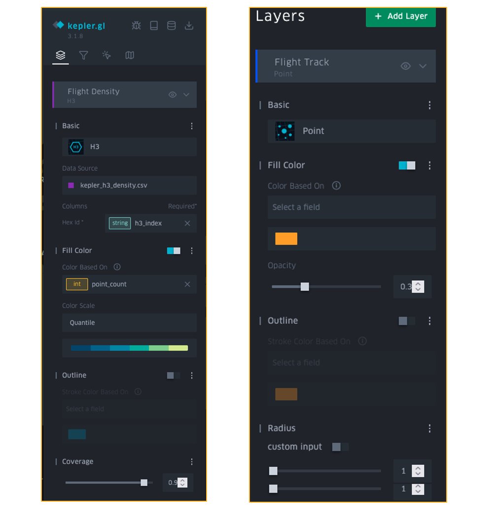
In Basic, choose H3 as the layer type, then add the following configuration:
Layer Name: Flight Density
Data Source: kepler_h3_density.csv
Hex ID: h3_index
In the Fill Color section:
Color: point_count
Color Scale: Quantile.
Color Range: Choose a blue/green gradient.
Set Opacity to 0.7.
In the Coverage section, set it to 0.9.
Create the Flight Tracks Layer:
Choose Add Layer in the left panel.
In Basic, choose Point as the layer type, then add the following configuration:
Layer Name: Flight Tracks
Data Source: kepler_track_points_sample.csv
Columns:
Latitude: lat
Longitude: lon
In the Fill Color section:
Solid Color: Orange
Opacity: 0.3
Set the Point’s Radius to 1
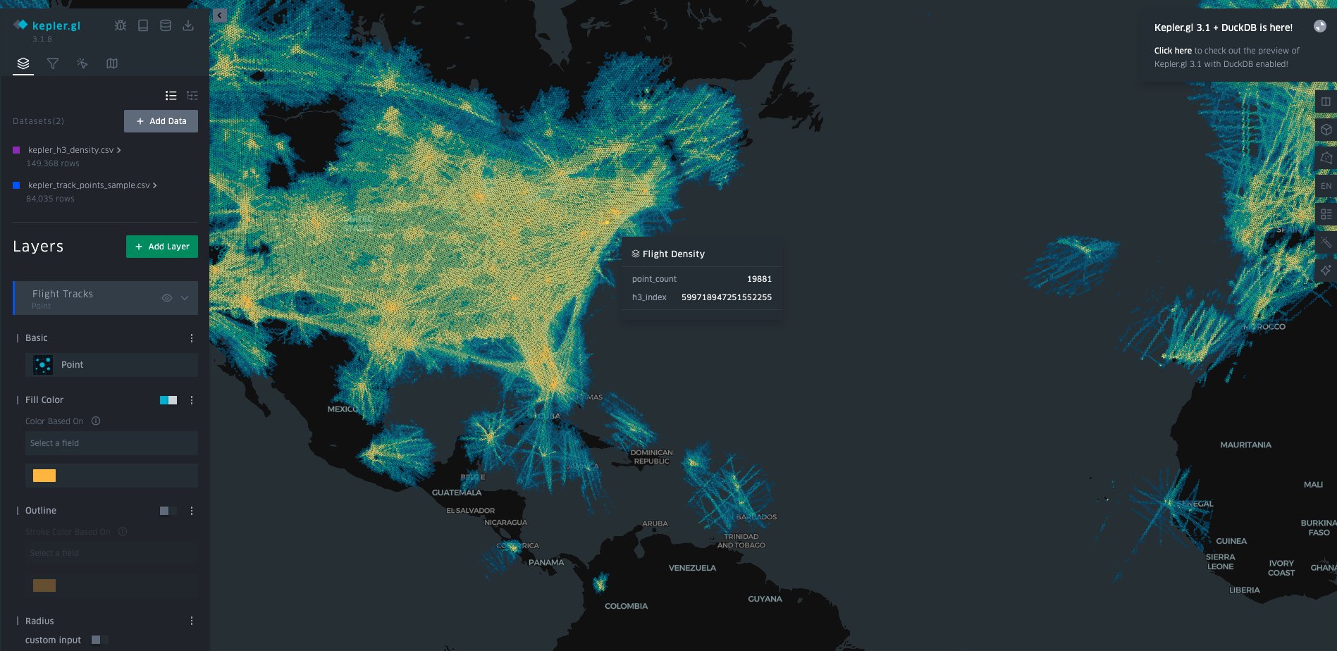
The layers should look similar to the following figure.
The graph visualization should now show flight density through color-coded hexagons, with individual flight tracks visible as orange points:
There you go! Now that you have knowledge about geospatial data and have created your first use case, take the opportunity to do some analysis and learn some interesting facts about flight patterns.
It is possible to experiment with other interesting types of analysis in Kepler.gl, such as Time Playback.
Clean up
To clean up your resources, complete the following tasks:
Delete the AWS Glue job process_sedona_geo_track.
Delete content from the Amazon S3 buckets: blog-sedona-artifacts-<account_number>-<aws_region> and blog-sedona-nessie-<account_number>-<aws_region>.
Conclusion
In this post, we showed how processing geospatial data can present significant challenges due to its complex nature (from big data to data structure format). For this use case of flight trackers, it involves vast amounts of information across multiple dimensions such as time, location, altitude, and flight paths, however, the combination of Spark’s distributed computing capabilities and Sedona’s optimized geospatial functions helps overcome those challenges. The spatial partitioning and indexing features of Sedona, coupled with Spark’s framework, enable us to perform complex spatial joins and proximity analyses efficiently, simplifying the overall data processing workflow.
The serverless nature of AWS Glue eliminates the need for managing infrastructure while automatically scaling resources based on workload demands, making it an ideal platform for processing growing volumes of flight data. As the volume of flight data grows or as processing requirements fluctuate, with AWS Glue, you can quickly adjust resources to meet demand, ensuring optimal performance without the need for cluster management.
By converting the processed results into CSV format and visualizing them in Kepler.gl, it is possible to create interactive visualizations that reveal patterns in flight paths, and you can efficiently analyze air traffic patterns, routes, and other insights. This end-to-end solution demonstrates how a modern data strategy in AWS with the support of open-source tools can transform raw geospatial data into actionable insights.
As your data and machine learning (ML) assets grow, tracking which assets lack documentation or monitoring asset registration trends becomes challenging without custom reporting infrastructure. You need visibility into your catalog’s health, without the overhead of managing ETL jobs. The metadata feature of Amazon SageMaker provides this capability to users. Converting catalog asset metadata into Apache Iceberg tables stored in Amazon S3 Tables removes the need to build and maintain custom ETL pipelines. Your team can then query asset metadata directly using standard SQL tools. You can now answer governance questions like asset registration trends, classification status, and metadata completeness using standard SQL queries through tools like Amazon Athena, Amazon SageMaker Unified Studio notebooks, and BIsystems.
This automated approach reduces ETL development time and gives your team visibility into catalog health, compliance gaps, and asset lifecycle patterns. The exported tables include technical metadata, business metadata, project ownership details, and timestamps, partitioned by snapshot date to enable time travel queries and historical analysis. Teams can use this capability to proactively monitor catalog health, identify gaps in documentation, track asset lifecycle patterns, and make sure that governance policies are consistently applied.
How metadata export works
After you enable the metadata export feature, it runs automatically on a daily schedule:
SageMaker Catalog creates the infrastructure — An Amazon Simple Storage Service (Amazon S3) table bucket named aws-sagemaker-catalog is created with an asset_metadata namespace and an empty asset table.
Daily snapshots are captured — A scheduled job runs once per day around midnight (local time per AWS Region) to export updated asset metadata.
Metadata is structured and partitioned — The export captures technical metadata (resource_id, resource_type), business metadata (asset_name, business_description), project ownership details, and timestamps, partitioned by snapshot_date for query performance.
Data becomes queryable — Within 24 hours, the asset table appears in Amazon SageMaker Unified Studio under the aws-sagemaker-catalog bucket and becomes accessible through Amazon Athena, Studio notebooks, or external BI tools.
Teams query using standard SQL — Data teams can now answer questions like “How many assets were registered last month?” or “Which assets lack business descriptions?” without building custom ETL pipelines.
The export evaluates catalog assets and their metadata properties in the domain, converting them into Apache Iceberg table format. The data flows into downstream analytics operations immediately, with no separate ETL or batch processes to maintain. The exported metadata becomes part of a queryable data lake that supports time-travel queries and historical analysis.
In this post, we demonstrate how to use the metadata export capability in Amazon SageMaker Catalog and perform analytics on these tables. We explore the following specific use-cases.
Audit historical changes to investigate what an asset looked like at a specific point in time.
Monitor asset growth view how the data catalog has grown over the last 30 days.
Track metadata improvements to see which assets gained descriptions or ownership over time.
Solution overview
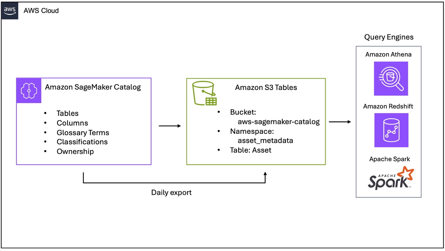
Figure 1 – SageMaker catalog export to S3 Tables
The architecture consists of three key components:
Amazon SageMaker Catalog exports asset metadata daily to Amazon S3.
S3 Tables stores metadata as Apache Iceberg tables in the aws-sagemaker-catalog bucket with ACID compliance and time travel.
Query engines (Amazon Athena, Amazon Redshift, and Apache Spark) access metadata using standard SQL from the asset_metadata.asset table.
What metadata is exposed?
SageMaker Catalog exports metadata in the asset_metadata.asset table:
Metadata Type
Fields
Description
Technical metadata
resource_id, resource_type_enum, account_id, region
Resource identifiers (ARN), types (GlueTable, RedshiftTable, S3Collection), and location
An Amazon SageMaker project for publishing assets.
For SageMaker Unified Studio domain setup instructions, refer to the SageMaker Unified Studio Getting started guide.
After you complete the prerequisites, complete the following steps.
Add this policy to our IAM user or role to enable metadata export. If using SageMaker Unified Studio to query the catalog, add this policy to the AmazonSageMakerAdminIAMExecutionRole managed role.
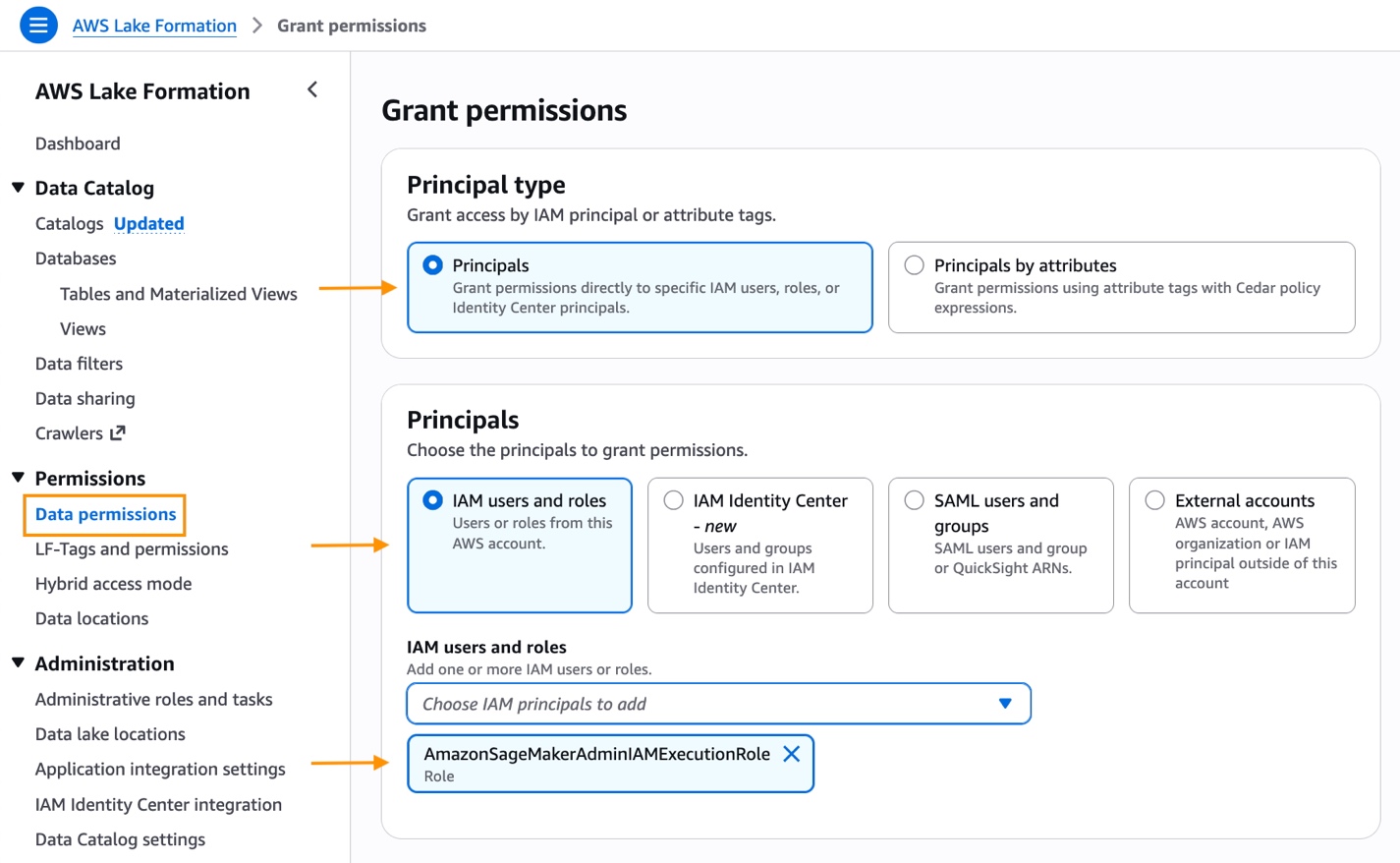
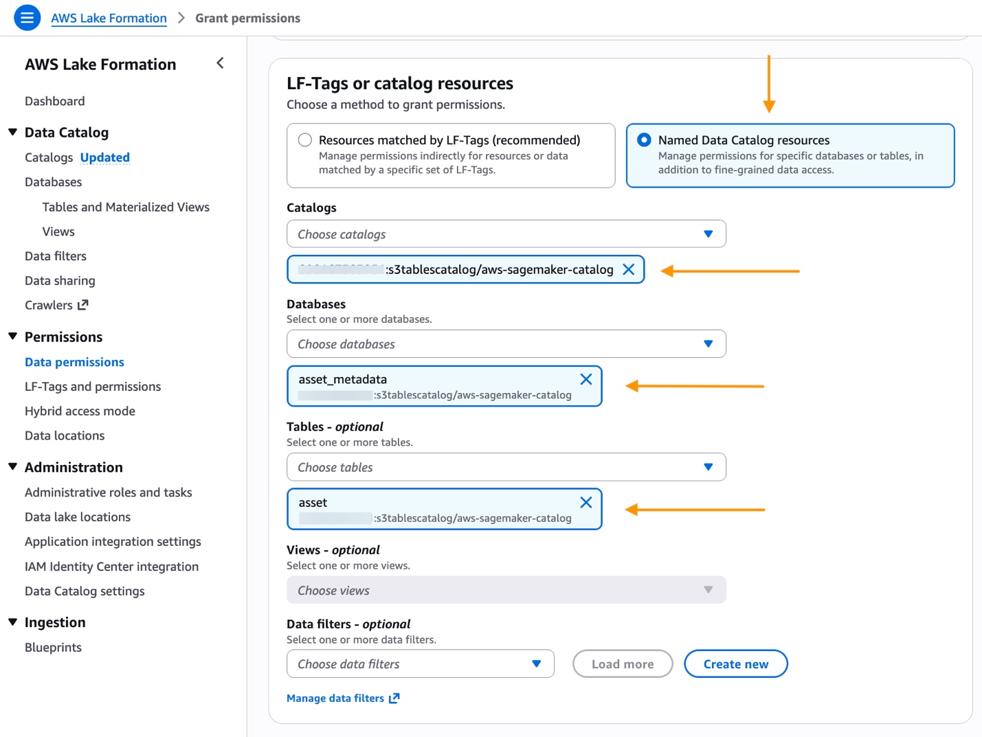
Grant describe and select permissions for SageMaker Catalog with AWS Lake Formation. This step can be performed in the AWS Lake Formation console.
Select Permissions -> Data permissions and choose Grant.
Figure 2 – AWS Lake Formation grant permission
Under Principal type, select Principals, IAM users and roles and the AWS managed AmazonSageMakerAdminIAMExecutionRole execution role.
Choose Named Data Catalog resources.
Under Catalogs, search for and select <account-id>:s3tablecatalog/aws-sagemaker-catalog.
Under Databases, select asset_metadata database.
Figure 3 – AWS Lake Formation catalog, database, and table
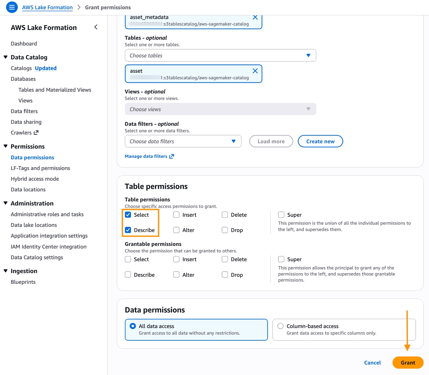
Figure 4 – AWS Lake Formation grant permission
For Table, select asset.
Under Table permissions, check Select and Describe.
Choose Grant to save the permissions.
Enable data export using the AWS CLI
Configure metadata export using the PutDataExportConfiguration API. The Amazon DataZone service automatically creates an S3 table bucket named aws-sagemaker-catalog with an asset_metadata namespace, and schedules a daily export job. Asset metadata is exported once daily around midnight local time per AWS Region.
The SageMaker Domain identifier is available on domain detail page in the AWS Management Console. Accessing the asset table through the S3 Tables console or the Data tab in SageMaker Unified Studio can require up to 24 hours.
AWS CLI command to enable SageMaker catalog export:
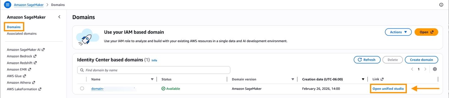
Navigate to Amazon SageMaker Domains in the AWS Management Console.
Select your domain and select Open.
Figure 5 – Open Amazon SageMaker Unified Studio
In SageMaker Unified Studio, choose a project from the Select a project dropdown list.
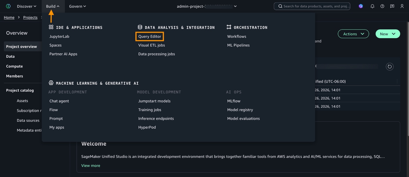
To query SageMaker catalog data, select Build in the menu bar and then choose Query Editor. To create a new project, follow the instructions in the Amazon SageMaker Unified Studio User Guide.
Figure 6 – Open SageMaker Unified Studio Query Editor
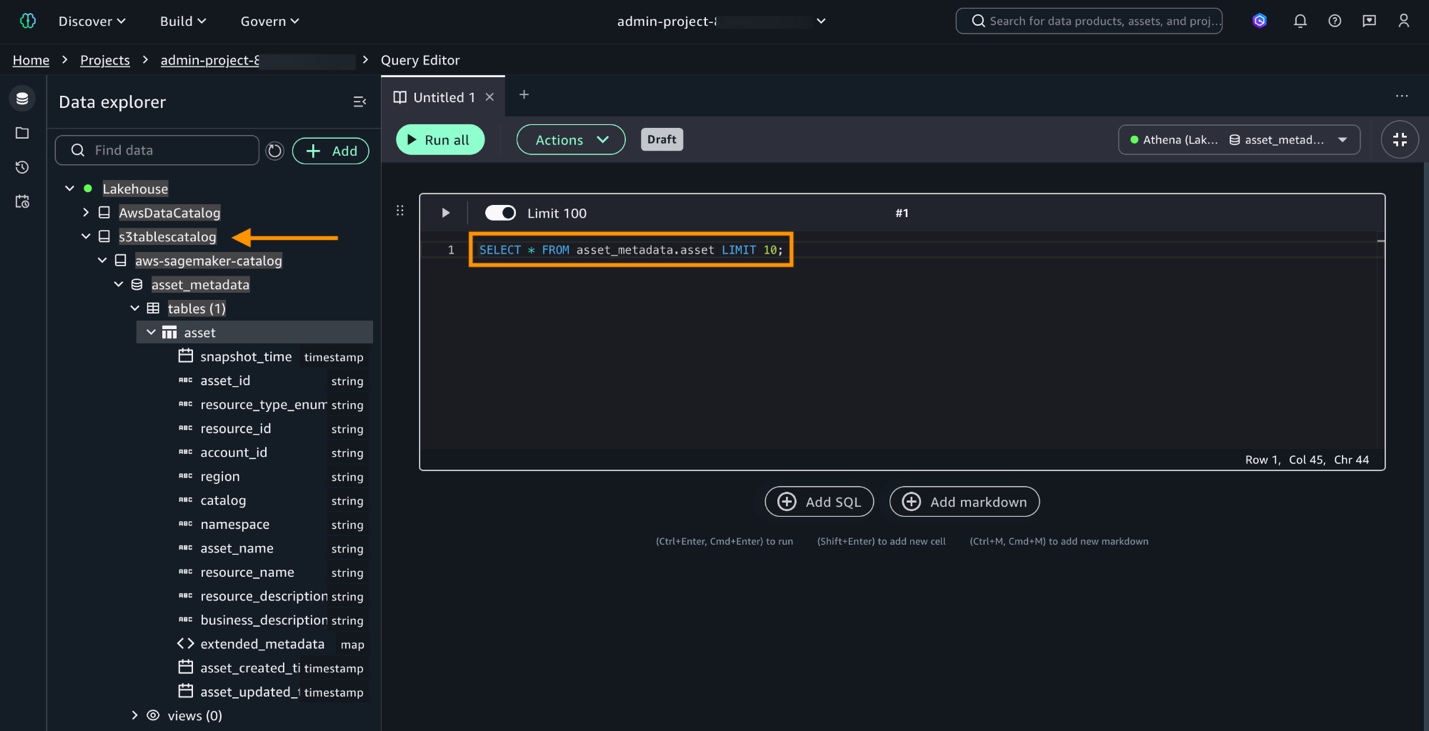
The asset_metadata.asset table is available in Data explorer. Use Data explorer to view the schema and query data to perform analytics from.
Expand Catalogs in Data explorer. Then, select and expand s3tablecatalog, aws-sagemaker-catalog, asset_metadata, and asset.
Test querying the catalog with SELECT * FROM asset_metadata.asset LIMIT 10;.
Figure 7 – Query SageMaker catalog
Queries for observability and analytics
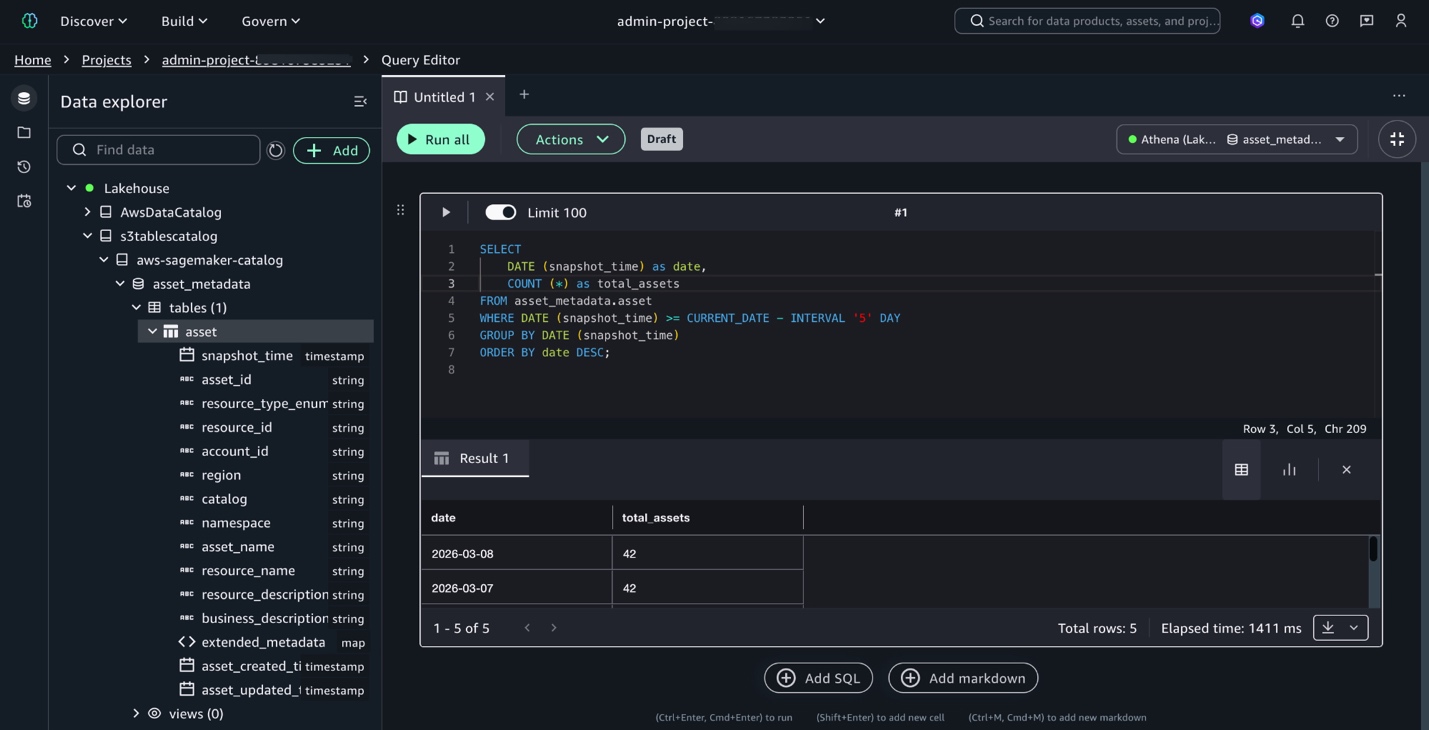
With setup complete, execute queries to gain insights on catalog usage and changes. To monitor asset growth, and view how the data catalog has grown over the last five days:
SELECT
    DATE (snapshot_time) as date,
    COUNT (*) as total_assets
FROM asset_metadata.asset
WHERE
     DATE (snapshot_time) >= CURRENT_DATE - INTERVAL '5' DAY
GROUP BY DATE (snapshot_time)
ORDER BY date DESC;
Figure 8 – Query asset growth
Use the catalog to track metadata changes to determine which assets gained descriptions or ownership over time. Use this query to identify assets that gained business descriptions over the past five days by comparing today’s snapshot with the earlier snapshot.
SELECT
    t.asset_id,
    t.resource_name,
    p.business_description as description_before,
    t.business_description as description_now
FROM asset_metadata.asset t
JOIN asset_metadata.asset p ON t.asset_id = p.asset_id
WHERE DATE(t.snapshot_time) = CURRENT_DATE
    AND DATE(p.snapshot_time) = CURRENT_DATE - INTERVAL '5' DAY
    AND p.business_description IS NULL
    AND t.business_description IS NOT NULL;
Investigate asset values at a specific point in time using this query to retrieve metadata from any snapshot date.
SELECT
     asset_id,
     resource_name,
     business_description,
     extended_metadata['owningEntityId'] as owner,
     snapshot_time
FROM asset_metadata.asset
WHERE asset_id = 'your-asset-id'
     AND DATE(snapshot_time) = DATE('2025-11-26');
Clean up resources
To avoid ongoing charges, clean up the resources created in this walkthrough:
Disable metadata export:
Disable the daily metadata export to stop new snapshots:
Optionally, delete the S3 Tables namespace containing the exported metadata to remove historical snapshots and stop storage charges. For instructions on how to delete S3 tables, see Deleting an Amazon S3 table in the Amazon Simple Storage Service User Guide.
Conclusion
In this post, you enabled the metadata export feature of SageMaker Catalog and used SQL queries to gain visibility into your asset inventory. The feature converts asset metadata into Apache Iceberg tables partitioned by snapshot date, so you can perform time-travel queries, monitor catalog growth, track metadata completeness, and audit historical asset states. This provides a repeatable, low-overhead way to maintain catalog health and meet governance requirements over time.
This post is cowritten by Anil Akarsu and Dr. Renè Holschuh from BASF.
BASF is a global chemical industry leader and active member of the Catena-X Automotive Network. It pioneers sustainable solutions that enable automotive organizations to track carbon emissions across complex supply chains. CircularTree transforms sustainability reporting through innovative digital solutions that systematically identify and control Scope 3 greenhouse gas (GHG) emissions across global supply networks. They establish standardized data exchange protocols through participation in forward-thinking associations including PACT, Catena-X, and ESTAINIUM. BASF and CircularTree created PACIFIC, a product powered by AWS that streamlines transparent product carbon footprint (PCF) reporting across the value chain by automating PCF data exchange, reducing manual effort, and ensuring trustworthy data sharing. Through this unique relationship, AWS helps customers integrate software, services, and processes to accelerate business transformation. This post explores how PACIFIC enables multi-tenant, sovereign PCF exchange on the Catena-X data space using Amazon Elastic Container Service (Amazon ECS) on AWS Fargate, Amazon Cognito, and AWS Identity and Access Management (IAM) to deliver measurable environmental impact and competitive advantage in a carbon-conscious marketplace.
Carbon data at scale, across company borders
Sustainability is now an operational requirement, driven by growing regulatory pressure in the European Union and increasing customer expectations for credible and auditable emissions data. For manufacturers in the automotive supply chain, this is especially challenging because emissions data does not live in one place. It is distributed across fragmented tiers of suppliers, different internal systems, and partner-to-partner handoffs that still happen through spreadsheets, emails, and one-off integrations.
At the same time, the industry is converging on shared ways to exchange data, with Catena-X setting expectations for interoperability and trust in cross-company collaboration. PACIFIC was built for this reality as a multi-tenant SaaS product that enables companies to manage and exchange PCFs while maintaining data sovereignty. Its Catena-X certification signals alignment with industry standards, and the partnership with BASF grounds the platform in real supply chain requirements.
Data security, sovereignty, and interoperability
To make PCF exchange work in the real world, PACIFIC needed to solve two problems at the same time: enable frictionless collaboration across companies, while guaranteeing that each company stays in full control of their data and credentials. The platform had to operate as a multi-tenant software as a service (SaaS) for the supply chain, serving organizations on shared infrastructure without introducing any possibility of cross-tenant access.
They had to build an interoperable solution that could communicate with other solution providers on the Catena-X data space, using Eclipse Dataspace Components (EDC) connectors as a standard mechanism for cross-company data exchange. That meant enforcing strict data sovereignty, not only for PCF records but also for sensitive Catena-X integration configuration such as EDC and Digital Twin Registry (DTR) credentials. At the exchange layer, PACIFIC needed end-to-end authorization aligned with Catena-X expectations, where PCF data is shared only after explicit agreement and policy negotiation through EDC. Finally, the solution had to be practical to run and scale, so the following had to happen:
Onboard new companies without spinning up separate AWS accounts per tenant
Integrate suppliers’ PCF systems like BASF without tight coupling to the exchange workflow
Keep the platform secure, auditable, and operable as usage grows
Solution overview
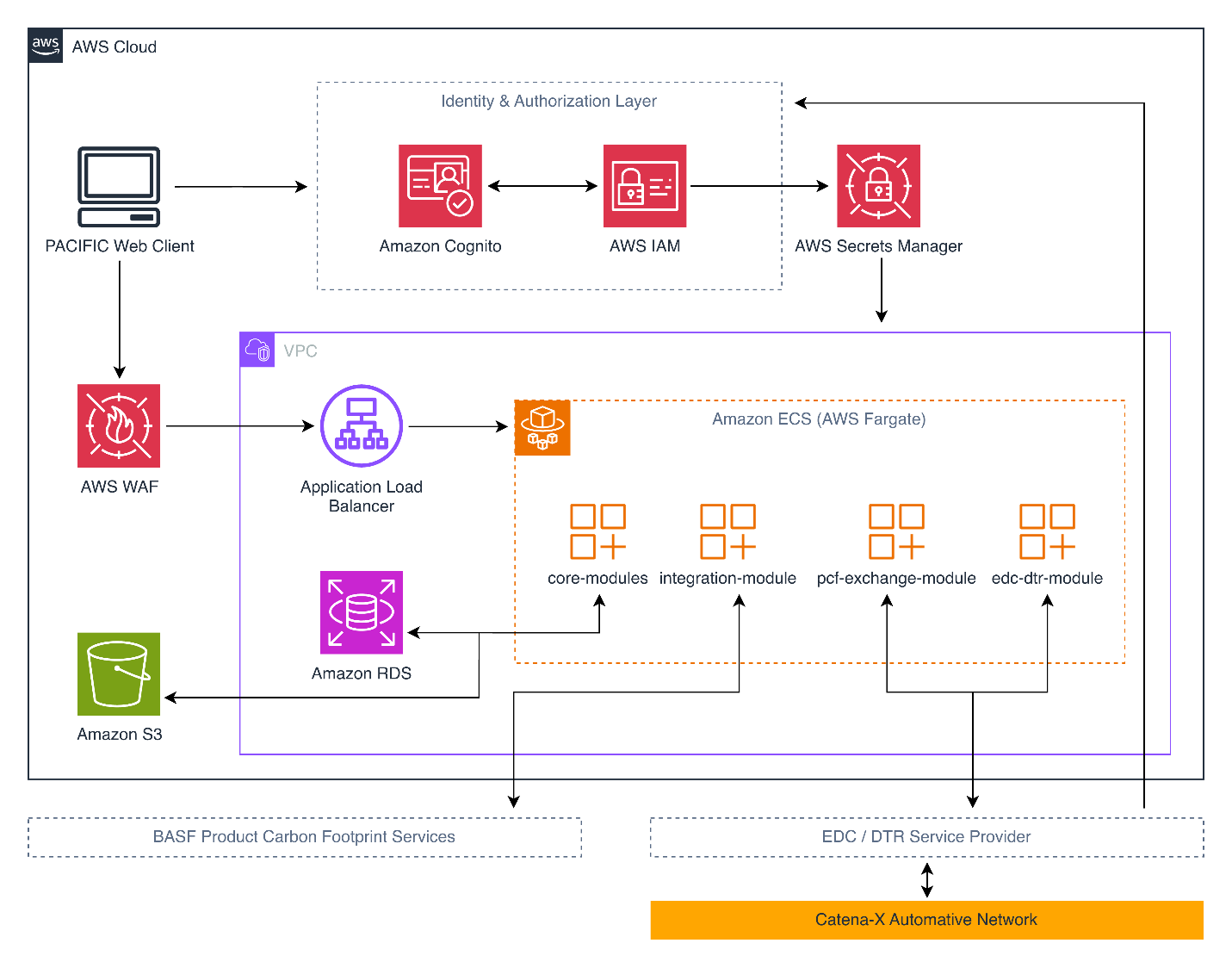
Figure 1 gives a high-level view of how PACIFIC is built and deployed to enable secure, multi-tenant PCF exchange on the Catena-X data space. It shows the main building blocks of the product, how user traffic reaches the application, how tenant-aware identity and authorization are enforced, and how PACIFIC separates core platform features from integrations and exchange endpoints. The diagram also highlights the external connections enabling interoperability, including supplier PCF data sources like BASF services, and EDC and DTR “enablement service providers” for Catena-X based data sharing.
Figure 1: PACIFIC high-level service architecture
Data protection through IAM-based tenant isolation
A core requirement for PACIFIC is maintaining data protection and security. Each company must have exclusive control over their PCF data, EDC connector, and DTR management credentials, without any possibility of cross-tenant access. Rather than provisioning separate AWS accounts per tenant PACIFIC implements a fine-grained IAM-based isolation model built on Amazon Cognito and AWS Secrets Manager. When a company joins the platform, PACIFIC automatically provisions a dedicated IAM role with a scoped policy that permits access only to that company’s secrets in Secrets Manager. Users are assigned to an Amazon Cognito user pool group linked to their company’s IAM role. When a user authenticates, the Amazon Cognito identity pool maps their group membership to the corresponding IAM role, and AWS Security Token Service (AWS STS) issues temporary credentials for that role. This means, a user’s credentials can only retrieve their own company’s EDC secrets and access to other tenants’ configuration is denied at the IAM policy level. This architecture delivers true multi-tenant isolation using native AWS identity services, without the overhead of managing dedicated accounts or Amazon Virtual Private Cloud (Amazon VPC) per customer.
Securing PCF exchange with EDC-issued authorization tokens
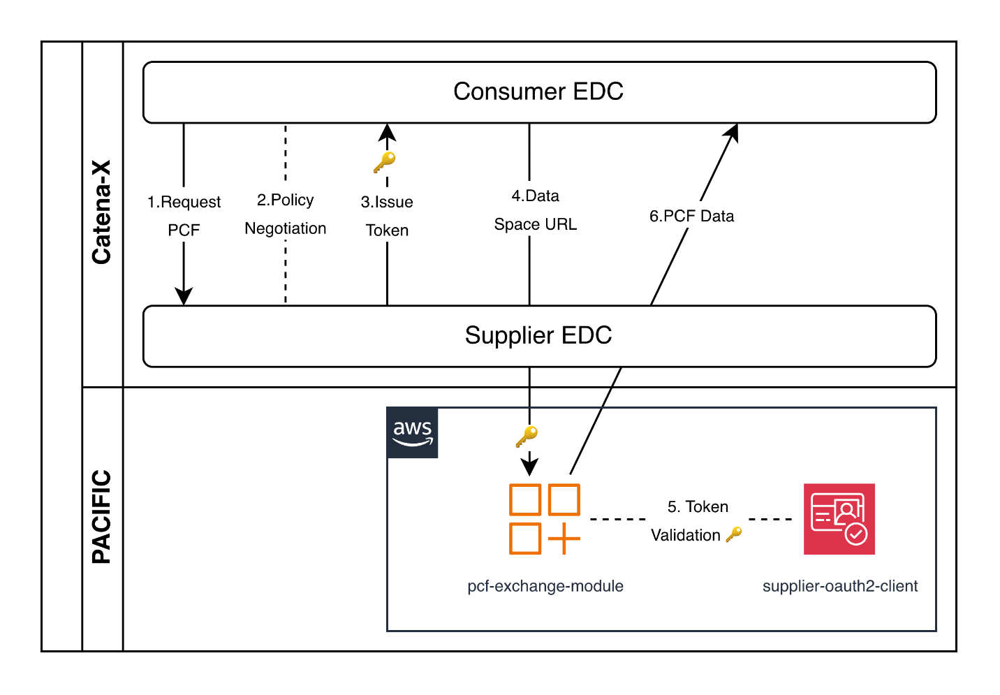
Beyond tenant isolation within PACIFIC, CircularTree enforces authorization at the data exchange layer through the pcf-exchange-module, a per-tenant endpoint that serves PCF data to authorized trading partners. When a consumer’s EDC connector requests PCF data from a supplier’s EDC, the two connectors negotiate and agree on usage policies governing how the exchanged information can be used. After this agreement is established, the supplier’s EDC issues a special authorization token to the consumer’s EDC. The token derives from the supplier company’s Cognito app client credentials stored within their EDC and grants access specifically to that supplier’s pcf-exchange-module endpoint in PACIFIC. The consumer’s EDC then uses this token to call the supplier’s dedicated endpoint and retrieve the authorized PCF data. Because each tenant’s pcf-exchange-module is published as an individual endpoint, which only accepts tokens issued through the EDC handshake process, unauthorized access is prevented at multiple levels. One level is through EDC policy negotiation, and the other is through company-scoped OAuth2 token validation. This ensures that PCF data is transmitted only after explicit consent and only to the specific trading partner authorized in the data exchange agreement. Figure 2 gives an overview of the communication flow.
Figure 2: EDC-to-EDC communication with Cognito Oauth2 Tokens
Integrating supplier PCF systems through the integration module
While the pcf-exchange-module handles secure data exchange between trading partners using the Catena-X data space, PACIFIC also needs to ingest PCF data from suppliers’ internal systems. Running on AWS Fargate, the integration-module provides a flexible, scalable integration layer that connects to proprietary supplier PCF systems, such as BASF’s internal PCF services. Each supplier integration requires handling unique authentication flows. This ranges from OAuth2 client credentials to certificate-based authentication or API key mechanisms, all of which are securely managed through AWS Secrets Manager. The integration-module expects incoming PCF data to already conform to the standardized Catena-X PCF JSON format, ensuring consistency at the point of ingestion. After received, PCF data is stored in Amazon Simple Storage Service (Amazon S3) under company-specific prefixes. This is where IAM policies make sure that only the PCF owner company can access their respective data. By decoupling supplier system integration from the data exchange layer, PACIFIC can onboard new supplier PCF data sources without impacting the downstream Catena-X data sharing workflows. This can be done while the S3-based storage model helps maintain strict data sovereignty, and each company’s PCF data remains isolated and accessible only to its rightful owner.
Conclusion
PACIFIC turns Catena-X PCF exchange from a specification into an interoperable, scalable workflow running on Amazon ECS and AWS Fargate without requiring companies to give up control of their data and credentials. The impact is measurable in both speed and operational scalability. From a business perspective, BASF highlights the most tangible improvement: when a requested PCF dataset is already available, a manual exchange can take up to around seven days, whereas PACIFIC responds in seconds, and can deliver automated updates when PCFs change. This capability delivers up to 75% time savings for both customers and BASF. It also reduces the time-to-data from days to seconds and making emissions information more visible and usable in day-to-day supply chain operations. PACIFIC’s multi-tenant architecture scales onboarding and operations without managing individual AWS accounts per company, while still enforcing strong tenant isolation through IAM-scoped access control and per-tenant exchange endpoints. This scalability translates into faster onboarding, enabling BASF to integrate significantly more partners into the data space. The results are measurable: an 80% increase in newly onboarded companies between 2024 and 2025, and 55% growth in requested products and shared PCFs over the same period. This provides a scalable baseline for expanding the number of onboarded organizations and increasing the volume of PCF data exchanged as adoption grows—without weakening data sovereignty or interoperability. These results underline PACIFIC’s role as a catalyst for accelerating decarbonization across supply chains.
We encourage you to join BASF, CircularTree, and AWS in industry data sharing through emerging data spaces and transparent, trusted PCF exchange across global supply networks. To explore more sustainability solutions and AWS architecture patterns, visit the AWS Architecture Blog and get started with PACIFIC through the Cofinity-X App Marketplace.
Efforts to introduce malicious code into the open-source supply
chain have been on the rise in recent years, and there is no indication that they
will abate anytime soon. These attacks are often found quickly, but not quickly
enough to prevent the compromised code from being automatically injected into other
projects or code deployed by users where it can wreak havoc. One method of avoiding
supply-chain attacks is to add a delay of a few days before pulling upates in what
is known as a “dependency cooldown”. That tactic is starting to find favor with
users and some language ecosystem package managers. While this practice is
considered a reasonable response by many, others are complaining that those
employing dependency cooldowns are free-riding on the larger community by letting
others take the risk.
In Rust, types either possess a constant size known at compile time, or a
dynamically calculated size known at
run time. That is fine for most purposes, but recent proposals for the language
have shown the need for a more fine-grained hierarchy.
RFC 3729 from David Wood and Rémy Rakic would add a hierarchy of
traits to describe types with sizes known under different circumstances. While
the idea has been subject to discussion for many years, a growing number of
use cases for the feature have come to light.
Version
2.26.0 of the LilyPond
music-engraving program has been released. Major
changes include the ability to use the Cairo library to generate
output and improvements in spacing between clefs and time
signatures. See the release notes for a full list of miscellaneous
improvements as well as what’s new with musical
and specialist
notation.
Greg Kroah-Hartman has announced the release of the 7.0.1, 6.19.14, 6.18.24, and 6.12.83 stable kernels. As usual, each
contains important fixes throughout the tree. Users are encouraged to
upgrade.
Rust Workers run on the Cloudflare Workers platform by compiling Rust to WebAssembly, but as we’ve found, WebAssembly has some sharp edges. When things go wrong with a panic or an unexpected abort, the runtime can be left in an undefined state. For users of Rust Workers, panics were historically fatal, poisoning the instance and possibly even bricking the Worker for a period of time.
While we were able to detect and mitigate these issues, there remained a small chance that a Rust Worker would unexpectedly fail and cause other requests to fail along with it. An unhandled Rust abort in a Worker affecting one request might escalate into a broader failure affecting sibling requests or even continue to affect new incoming requests. The root cause of this was in wasm-bindgen, the core project that generates the Rust-to-JavaScript bindings Rust Workers depend on, and its lack of built-in recovery semantics.
In this post, we’ll share how the latest version of Rust Workers handles comprehensive Wasm error recovery that solves this abort-induced sandbox poisoning. This work has been contributed back into wasm-bindgen as part of our collaboration within the wasm-bindgen organization formed last year. First with panic=unwind support, which ensures that a single failed request never poisons other requests, and then with abort recovery mechanisms that guarantee Rust code on Wasm can never re-execute after an abort.
Initial recovery mitigations
Our initial attempts to address reliability in this area focused on understanding and containing failures caused by Rust panics and aborts in production Rust Workers. We introduced a custom Rust panic handler that tracked failure state within a Worker and triggered full application reinitialization before handling subsequent requests. On the JavaScript side, this required wrapping the Rust-JavaScript call boundary using Proxy‑based indirection to ensure that all entrypoints were consistently encapsulated. We also made targeted modifications to the generated bindings to correctly reinitialize the WebAssembly module after a failure.
While this approach relied on custom JavaScript logic, it demonstrated that reliable recovery was achievable and eliminated the persistent failure modes we were seeing in practice. This solution was shipped by default to all workers‑rs users starting in version 0.6, and it laid the groundwork for the more general, upstreamed abort recovery mechanisms described in the sections that follow.
Implementing panic=unwind with WebAssembly Exception Handling
The abort recovery mechanisms described above ensure that a Worker can survive a failure, but they do so by reinitializing the entire application. For stateless request handlers, this is fine. But for workloads that hold meaningful state in memory, such as Durable Objects, reinitialization means losing that state entirely. A single panic in one request could wipe the in-memory state being used by other concurrent requests.
In most native Rust environments, panics can be unwound, allowing destructors to run and the program to recover without losing state. In WebAssembly, things historically looked very different. Rust compiled to Wasm via wasm32-unknown-unknown defaults to panic=abort, so a panic inside a Rust Worker would abruptly trap with an unreachable instruction and exit Wasm back to JS with a WebAssembly.RuntimeError.
To recover from panics without discarding instance state, we needed panic=unwind support for wasm32-unknown-unknown in wasm-bindgen, made possible by the WebAssembly Exception Handling proposal, which gained wide engine support in 2023.
We start by compiling with RUSTFLAGS='-Cpanic=unwind' cargo build -Zbuild-std, which rebuilds the standard library with unwind support and generates code with proper panic unwinding. For example:
struct HasDropA;
struct HasDropB;
extern "C" {
    fn imported_func();
}

fn some_func() {
    let a = HasDropA;
    let b = HasDropB;
    imported_func();
}
This ensures that even if imported_func() panics, destructors still run. Similarly, std::panic::catch_unwind(|| some_func()) compiles into:
try
  call <some_func>
  ;; set result to Ok(return value)
catch
  try
    call <std::panicking::catch_unwind::cleanup>
    ;; set result to Err(panic payload)
  catch_all
    call <core::panicking::cannot_unwind>
    unreachable
  end
end
Getting this to work end-to-end required several changes to the wasm-bindgen toolchain. The WebAssembly parser Walrus did not know how to handle try/catch instructions, so we added support for them. The descriptor interpreter also needed to be taught how to evaluate code containing exception handling blocks. At that point, the full application could be built with panic=unwind.
The final step was modifying the exports generated by wasm-bindgen to catch panics at the Rust-JavaScript boundary and surface them as JavaScript PanicError exceptions. One subtlety: Rust will catch foreign exceptions and abort when unwinding through extern "C" functions, so exports needed to be marked extern "C-unwind" to explicitly allow unwinding across the boundary. For futures, a panic rejects the JavaScript Promise with a PanicError.
Closures required special attention to ensure unwind safety was properly checked, via a new MaybeUnwindSafe trait that checks UnwindSafe only when built with panic=unwind. This quickly exposed a problem, though: many closures capture references that remain after an unwind, making them inherently unwind-unsafe. To avoid a situation where users are encouraged to incorrectly wrap closures in AssertUnwindSafe just to satisfy the compiler, we added Closure::new_aborting variants, which terminate on panic instead of unwinding in cases where unwind safety can’t be guaranteed.
With panic unwinding enabled:
Panics in exported Rust functions are caught by wasm-bindgen
Panics surface to JavaScript as PanicError exceptions
Async exports reject their returned promises with a PanicError
Rust destructors run correctly
The WebAssembly instance remains valid and reusable
The full details of the approach and how to use it in wasm-bindgen are covered in the latest guide page for Wasm Bindgen: Catching Panics.
Abort recovery
Even with panic=unwind support, aborts still happen – out-of-memory errors being one common cause. Because aborts can’t unwind, there is no possibility of state recovery at all, but we can at least detect and recover from aborts for future operations to avoid invalid state erroring subsequent requests.
Panic unwind support introduced a new problem for abort recovery. When we receive an error from Wasm we don’t know if it came from an extern “C-unwind” foreign error, or if it was a genuine abort. Aborts can take many shapes in WebAssembly.
We had two options to solve this technically: either mark all errors which are definitely aborts, or mark all errors which are definitely unwinds. Either could have worked but we chose the latter. Since our foreign exception handling was directly using raw WAT-level (WebAssembly text format) Exception Handling instructions already, we found it easier to implement exception tags for foreign exceptions to distinguish them from aborting non-unwind-safe exceptions.
With the ability to clearly distinguish between recoverable and non-recoverable errors thanks to this Exception.Tag feature in WebAssembly Exception Handling, we were able to then integrate both a new abort handler as well as abort reentrancy guards.
A new abort hook, set_on_abort, can be used at initialization time to attach a handler that recovers accordingly for the platform embedding’s needs.
Hardening panic and abort handling is critical to avoiding invalid execution state. WebAssembly allows deeply interleaved call stacks, where Wasm can call into JavaScript and JavaScript can re-enter Wasm at arbitrary depths, while alongside this, multiple tasks can be functioning in the same instance. Previously, an abort occurring in one task or nested stack was not guaranteed to invalidate higher stacks through JS, leading to undefined behavior. Care was required to ensure we can guarantee the execution model, and contribution in this space remains ongoing.
While aborts are never ideal, and reinitialization on failure is an absolute worst-case scenario, implementing critical error recovery as the last line of defense ensures execution correctness and that future operations will be able to succeed. The invalid state does not persist, ensuring a single failure does not cascade into multiple failures.
Extension: abort reinitialization for wasm-bindgen libraries
While we were working on this, we realized that this is a common problem for libraries used by JS that are built with wasm-bindgen, and that they would also benefit from attaching an abort handler to be able to perform recovery.
But when building Wasm as an ES module and importing it directly (e.g. via import { func } from ‘wasm-dep’), it’s not clear what the recovery mechanism would be for a Wasm abort while calling func() for an already-linked and initialized library that is in a user JS application.
While not strictly a Rust Workers use case, our team also supports JS-based Workers users who run Rust-backed Wasm library dependencies. If we could fix this problem at the same time, that could indirectly also benefit Wasm usage on the Cloudflare Workers platform.
To support automatic abort recovery for Wasm library use cases, we added support for an experimental reinitialization mechanism into wasm‑bindgen, --reset-state-function. This exposes a function that allows the Rust application to effectively request that it reset its internal Wasm instance back to its initial state for the next call, without requiring consumers of the generated bindings to reimport or recreate them. Class instances from the old instance will throw as their handles become orphaned, but new classes can then be constructed. The JS application using a Wasm library is errored but not bricked.
The full technical details of this feature and how to use it in wasm-bindgen are covered in the new wasm-bindgen guide section Wasm Bindgen: Handling Aborts.
Maturing the Rust Wasm Exception Handling ecosystem
Upstream contributions for this work did not stop at the wasm-bindgen project. Building for Wasm with panic=unwind still requires an experimental nightly Rust target, so we’ve also been working to advance Rust’s Wasm support for WebAssembly Exception Handling to help bring this to stable Rust.
During the development of WebAssembly Exception Handling, a late‑stage specification change resulted in two variants: legacy exception handling and the final modern exception handling “with exnref”. Today, Rust’s WebAssembly targets still default to emitting code for the legacy variant. While legacy exception handling is widely supported, it is now deprecated.
Modern WebAssembly Exception Handling is supported as of the following JS platform releases:
Runtime
Version
Release Date
v8
13.8.1
April 28, 2025
workerd
v1.20250620.0
June 19, 2025
Chrome
138
June 28, 2025
Firefox
131
October 1, 2024
Safari
18.4
March 31, 2025
Node.js
25.0.0
October 15, 2025
As we were investigating the support matrix, the largest concern ended up being the Node.js 24 LTS release schedule, which would have left the entire ecosystem stuck on legacy WebAssembly Exception Handling until April 2028.
Having discovered this discrepancy, we were able to backport modern exception handling to the Node.js 24 release, and even backport the fixes needed to make it work on the Node.js 22 release line to ensure support for this target. This should allow the modern Exception Handling proposal to become the default target next year.
Over the coming months, we’ll be working to make the transition to stable panic=unwind and modern Exception Handling as invisible as possible to end users.
While these long‑term investments in the ecosystem take time, they help build a stronger foundation for the Rust WebAssembly community as a whole, and we’re glad to be able to contribute to these improvements.
Using panic unwind in Rust Workers
As of version 0.8.0 of Rust Workers, we have a new --panic-unwind flag, which can be added to the build command, following the instructions here.
With this flag, panics can be fully recovered, and abort recovery will use the new abort classification and recovery hook mechanism. We highly recommend upgrading and trying it out for a more stable Rust Workers experience, and plan to make panic=unwind the default in a subsequent release. Users remaining on panic=abort will still continue to take advantage of the previous custom recovery wrapper handling from 0.6.0.
Committing to Rust Workers stability
This work is part of our ongoing effort towards a stable release for Rust Workers. By solving these sharp edges of the Wasm platform foundations at their root, and contributing back to the ecosystem where it makes sense, we build stronger foundations not just for our platform, but the entire Rust, JS, and Wasm ecosystem.
We have a number of future improvements planned for Rust Workers, and we’ll soon be sharing updates on this additional work, including wasm-bindgen generics and automated bindgen, which Guy Bedford from our team previewed in a talk on Rust & JS Interoperability at Wasm.io last month.
Find us in #rust‑on‑workers on the Cloudflare Discord. We also welcome feedback and discussion and especially all new contributors to the workers-rs and wasm-bindgen GitHub projects.
To provide the best experiences, we use technologies like cookies to store and/or access device information. Consenting to these technologies will allow us to process data such as browsing behavior or unique IDs on this site. Not consenting or withdrawing consent, may adversely affect certain features and functions.
Functional
Always active
The technical storage or access is strictly necessary for the legitimate purpose of enabling the use of a specific service explicitly requested by the subscriber or user, or for the sole purpose of carrying out the transmission of a communication over an electronic communications network.
Preferences
The technical storage or access is necessary for the legitimate purpose of storing preferences that are not requested by the subscriber or user.
Statistics
The technical storage or access that is used exclusively for statistical purposes.The technical storage or access that is used exclusively for anonymous statistical purposes. Without a subpoena, voluntary compliance on the part of your Internet Service Provider, or additional records from a third party, information stored or retrieved for this purpose alone cannot usually be used to identify you.
Marketing
The technical storage or access is required to create user profiles to send advertising, or to track the user on a website or across several websites for similar marketing purposes.