Build your next video application on Cloudflare

Post Syndicated from Jonathan Kuperman original https://blog.cloudflare.com/build-video-applications-cloudflare/

Build your next video application on Cloudflare

Build your next video application on Cloudflare

Historically, building video applications has been very difficult. There’s a lot of complicated tech behind recording, encoding, and playing videos. Luckily, Cloudflare Stream abstracts all the difficult parts away, so you can build custom video and streaming applications easily. Let’s look at how we can combine Cloudflare Stream, Access, Pages, and Workers to create a high-performance video application with very little code.

Today, we’re going to build a video application inspired by Cloudflare TV. We’ll have user authentication and the ability for administrators to upload recorded videos or livestream new content. Think about being able to build your own YouTube or Twitch using Cloudflare services!

Fetching a list of videos

On the main page of our application, we want to display a list of all videos. The videos are uploaded and stored with Cloudflare Stream, but more on that later! This code could be changed to display only the “trending” videos or a selection of videos chosen for each user. For now, we’ll use the search API and pass in an empty string to return all.

import { getSignedStreamId } from "../../src/cfStream"

export async function onRequestGet(context) {
    const {
        request,
        env,
        params,
    } = context

    const { id } = params

    if (id) {
        const res = await fetch(`https://api.cloudflare.com/client/v4/accounts/${env.CF_ACCOUNT_ID}/stream/${id}`, {
            method: "GET",
            headers: {
                "Authorization": `Bearer ${env.CF_API_TOKEN_STREAM}`
            }
        })

        const video = (await res.json()).result

        if (video.meta.visibility !== "public") {
            return new Response(null, {status: 401})
        }

        const signedId = await getSignedStreamId(id, env.CF_STREAM_SIGNING_KEY)

        return new Response(JSON.stringify({
            signedId: `${signedId}`
        }), {
            headers: {
                "content-type": "application/json"
            }
        })
    } else {
        const url = new URL(request.url)
        const res = await (await fetch(`https://api.cloudflare.com/client/v4/accounts/${env.CF_ACCOUNT_ID}/stream?search=${url.searchParams.get("search") || ""}`, {
            headers: {
                "Authorization": `Bearer ${env.CF_API_TOKEN_STREAM}`
            }
        })).json()

        const filteredVideos = res.result.filter(x => x.meta.visibility === "public") 
        const videos = await Promise.all(filteredVideos.map(async x => {
            const signedId = await getSignedStreamId(x.uid, env.CF_STREAM_SIGNING_KEY)
            return {
                uid: x.uid,
                status: x.status,
                thumbnail: `https://videodelivery.net/${signedId}/thumbnails/thumbnail.jpg`,
                meta: {
                    name: x.meta.name
                },
                created: x.created,
                modified: x.modified,
                duration: x.duration,
            }
        }))
        return new Response(JSON.stringify(videos), {headers: {"content-type": "application/json"}})
    }
}

We’ll go through each video, filter out any private videos, and pull out the metadata we need, such as the thumbnail URL, ID, and created date.

Playing the videos

To allow users to play videos from your application, they need to be public, or you’ll have to sign each request. Marking your videos as public makes this process easier. However, there are many reasons you might want to control access to your videos. If you want users to log in before they play them or the ability to limit access in any way, mark them as private and use signed URLs to control access. You can find more information about securing your videos here.

If you are testing your application locally or expect to have fewer than 10,000 requests per day, you can call the /token endpoint to generate a signed token. If you expect more than 10,000 requests per day, sign your own tokens as we do here using JSON Web Tokens.

Allowing users to upload videos

The next step is to build out an admin page where users can upload their videos. You can find documentation on allowing user uploads here.

This process is made easy with the Cloudflare Stream API. You use your API token and account ID to generate a unique, one-time upload URL. Just make sure your token has the Stream:Edit permission. We hook into all POST requests from our application and return the generated upload URL.

export const cfTeamsAccessAuthMiddleware = async ({request, data, env, next}) => {
    try {
        const userEmail = request.headers.get("cf-access-authenticated-user-email")

        if (!userEmail) {
            throw new Error("User not found, make sure application is behind Cloudflare Access")
        }
  
        // Pass user info to next handlers
        data.user = {
            email: userEmail
        }
  
        return next()
    } catch (e) {
        return new Response(e.toString(), {status: 401})
    }
}

export const onRequest = [
    cfTeamsAccessAuthMiddleware
]

The admin page contains a form allowing users to drag and drop or upload videos from their computers. When a logged-in user hits submit on the upload form, the application generates a unique URL and then posts the FormData to it. This code would work well for building a video sharing site or with any application that allows user-generated content.

async function getOneTimeUploadUrl() {
    const res = await fetch('/api/admin/videos', {method: 'POST', headers: {'accept': 'application/json'}})
    const upload = await res.json()
    return upload.uploadURL
}

async function uploadVideo() {
    const videoInput = document.getElementById("video");

    const oneTimeUploadUrl = await getOneTimeUploadUrl();
    const video = videoInput.files[0];
    const formData = new FormData();
    formData.append("file", video);

    const uploadResult = await fetch(oneTimeUploadUrl, {
        method: "POST",
        body: formData,
    })
}

Adding real time video with Stream Live

You can add a livestreaming section to your application as well, using Stream Live in conjunction with the techniques we’ve already covered.  You could allow logged-in users to start a broadcast and then allow other logged-in users, or even the public, to watch it in real-time! The streams will automatically save to your account, so they can be viewed immediately after the broadcast finishes in the main section of your application.

Securing our app with middleware

We put all authenticated pages behind this middleware function. It checks the request headers to make sure the user is sending a valid authenticated user email.

export const cfTeamsAccessAuthMiddleware = async ({request, data, env, next}) => {
    try {
        const userEmail = request.headers.get("cf-access-authenticated-user-email")

        if (!userEmail) {
            throw new Error("User not found, make sure application is behind Cloudflare Access")
        }
  
        // Pass user info to next handlers
        data.user = {
            email: userEmail
        }
  
        return next()
    } catch (e) {
        return new Response(e.toString(), {status: 401})
    }
}

export const onRequest = [
    cfTeamsAccessAuthMiddleware
]

Putting it all together with Pages

We have Cloudflare Access controlling our log-in flow. We use the Stream APIs to manage uploading, displaying, and watching videos. We use Workers for managing fetch requests and handling API calls. Now it’s time to tie it all together using Cloudflare Pages!

Pages provides an easy way to deploy and host static websites. But now, Pages seamlessly integrates with the Workers platform (link to announcement post). With this new integration, we can deploy this entire application with a single, readable repository.

Controlling access

Some applications are better public; others contain sensitive data and should be restricted to specific users. The main page is public for this application, and we’ve used Cloudflare Access to limit the admin page to employees. You could just as easily use Access to protect the entire application if you’re building an internal learning service or even if you want to beta launch a new site!

When a user clicks the admin link on our demo site, they will be prompted for an email address. If they enter a valid Cloudflare email, the application will send them an access code. Otherwise, they won’t be able to access that page.

Check out the source code and get started building your own video application today!

Архив на Wikileaks: САЩ: Радев е един от най-ангажиращите контакти на Посолството, Идва Промяна

Post Syndicated from Екип на Биволъ original https://bivol.bg/%D1%81%D0%B0%D1%89-%D1%80%D0%B0%D0%B4%D0%B5%D0%B2-%D0%B5-%D0%B5%D0%B4%D0%B8%D0%BD-%D0%BE%D1%82-%D0%BD%D0%B0%D0%B9-%D0%B0%D0%BD%D0%B3%D0%B0%D0%B6%D0%B8%D1%80%D0%B0%D1%89%D0%B8%D1%82%D0%B5-%D0%BA%D0%BE.html

петък 19 ноември 2021


Вчера и днес се появиха различни публикации тиражирани в някои сайтове и в социалните мрежи, относно присъствието на настоящия Президент и кандидат-президент Румен Радев в докладите на Посолството на САЩ…

Setting up EC2 Mac instances as shared remote development environments

Post Syndicated from Rick Armstrong original https://aws.amazon.com/blogs/compute/setting-up-ec2-mac-instances-as-shared-remote-development-environments/

This post is written by: Michael Meidlinger, Solutions Architect 

In December 2020, we announced a macOS-based Amazon Elastic Compute Cloud (Amazon EC2) instance. Amazon EC2 Mac instances let developers build, test, and package their applications for every Apple platform, including macOS, iOS, iPadOS, tvOS, and watchOS. Customers have been utilizing these instances in order to automate their build pipelines for the Apple platform and integrate their native build tools, such as Jenkins and GitLab.

Aside from build automation, more and more customers are looking to utilize EC2 Mac instances for interactive development. Several advantages exist when utilizing remote development environments over installations on local developer machines:

  • Light-weight process for rolling out consistent, up-to-date environments for every developer without having to install software locally.
  • Solve cross-platform issues by having separate environments for different target platforms, all of which are independent of the developer’s local setup.
  • Consolidate access to source code and internal build tools, as they can be integrated with the remote development environment rather than local developer machines.
  • No need for specialized or powerful developer hardware.

On top of that, this approach promotes cost efficiency, as it enables EC2 Mac instances to be shared and utilized by multiple developers concurrently. This is particularly relevant for EC2 Mac instances, as they run on dedicated Mac mini hosts with a minimum tenancy of 24 hours. Therefore, handing out full instances to individual developers is not practical most often.

Interactive remote development environments are also facilitated by code editors, such as VSCode, which provide a modern GUI based experience on the developer’s local machine while having source code files and terminal sessions for testing and debugging in the remote environment context.

This post will demonstrate how EC2 Mac instances can be setup as remote development servers that can be accessed by multiple developers concurrently in order to compile and run their code interactively via command line access. The proposed setup features centralized user management based on AWS Directory Service and shared network storage utilizing Amazon Elastic File System (Amazon EFS), thereby decoupling those aspects from the development server instances. As a result, new instances can easily be added when needed, and existing instances can be updated to the newest OS and development toolchain version without affecting developer workflow.

Architecture

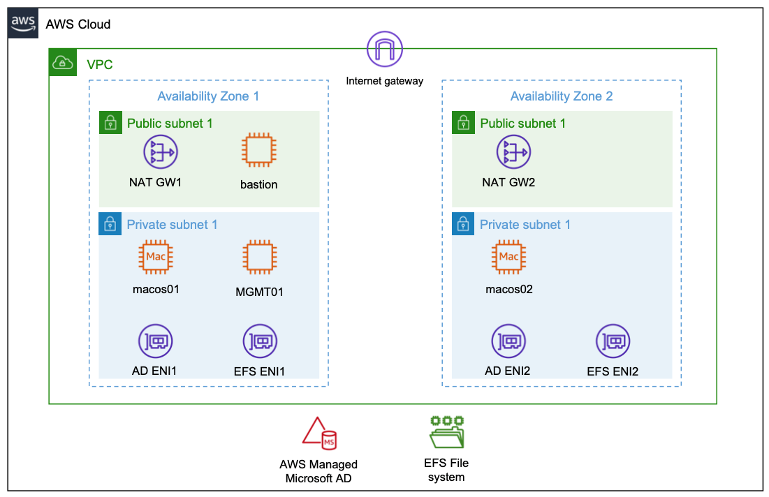
The following diagram shows the architecture rolled out in the context of this blog.

Architecture Diagram. A detailed description is featured in the blog text.

Compute Layer

The compute layer consists of two EC2 Mac instances running in isolated private subnets in different Availability Zones. In a production setup, these instances are provisioned with every necessary tool and software needed by developers to build and test their code for Apple platforms. Provisioning can be accomplished by creating custom Amazon Machine Images (AMIs) for the EC2 Mac instances or by bootstrapping them with setup scripts. This post utilizes Amazon provided AMIs with macOS BigSur without custom software. Once setup, developers gain command line access to the instances via SSH and utilize them as remote development environments.

Storage Layer

The architecture promotes the decoupling of compute and storage so that EC2 Mac instances can be updated with new OS and/or software versions without affecting the developer experience or data. Home directories reside on a highly available Amazon EFS file system, and they can be consistently accessed from all EC2 Mac instances. From a user perspective, any two EC2 Mac instances are alike, in that the user experiences the same configuration and environment (e.g., shell configurations such as .zshrc, VSCode remote extensions .vscode-server, or other tools and configurations installed within the user’s home directory). The file system is exposed to the private subnets via redundant mount target ENIs and persistently mounted on the Mac instances.

Identity Layer

For centralized user and access management, all instances in the architecture are part of a common Active Directory domain based on AWS Managed Microsoft AD. This is exposed via redundant ENIs to the private subnets containing the Mac instances.

To manage and configure the Active Directory domain, a Windows Instance (MGMT01) is deployed. For this post, we will connect to this instance for setting up Active Directory users. Note: other than that, this instance is not required for operating the solution, and it can be shut down both for reasons of cost efficiency and security.

Access Layer

The access layer constitutes the entry and exit point of the setup. For this post, it is comprised of an internet-facing bastion host connecting authorized Active Directory users to the Mac instances, as well as redundant NAT gateways providing outbound internet connectivity.

Depending on customer requirements, the access layer can be realized in various ways. For example, it can provide access to customer on-premises networks by using AWS Direct Connect or AWS Virtual Private Network (AWS VPN), or to services in different Virtual Private Cloud (VPC) networks by using AWS PrivateLink. This means that you can integrate your Mac development environment with pre-existing development-related services, such as source code and software repositories or build and test services.

Prerequisites

We utilize AWS CloudFormation to automatically deploy the entire setup in the preceding description. All templates and code can be obtained from the blog’s GitHub repository. To complete the setup, you need

Warning: Deploying this example will incur AWS service charges of at least $50 due to the fact that EC2 Mac instances can only be released 24 hours after allocation.

Solution Deployment

In this section, we provide a step-by-step guide for deploying the solution. We will mostly rely on AWS CLI and shell scripts provided along with the CloudFormation templates and use the AWS Management Console for checking and verification only.

1. Get the Code: Obtain the CloudFormation templates and all relevant scripts and assets via git:

git clone https://github.com/aws-samples/ec2-mac-remote-dev-env.git
cd ec2-mac-remote-dev-env
git submodule init 
git submodule update

2. Create an Amazon Simple Storage Service (Amazon S3) deployment bucket and upload assets for deployment: CloudFormation templates and other assets are uploaded to this bucket in order to deploy them. To achieve this, run the upload.sh script in the repository root, accepting the default bucket configuration as suggested by the script:

./upload.sh

3. Create an SSH Keypair for admin Access: To access the instances deployed by CloudFormation, create an SSH keypair with name mac-admin, and then import it with EC2:

ssh-keygen -f ~/.ssh/mac-admin
aws ec2 import-key-pair \
    --key-name "mac-admin" \
    --public-key-material fileb://~/.ssh/mac-admin.pub

4. Create CloudFormation Parameters file: Initialize the json file by copying the provided template parameters-template.json :

cp parameters-template.json parameters.json

Substitute the following placeholders:

a. <YourS3BucketName>: The unique name of the S3 bucket you created in step 2.

b. <YourSecurePassword>: Active Directory domain admin password. This must be 8-32 characters long and can contain numbers, letters and symbols.

c. <YourMacOSAmiID>: We used the latest macOS BigSur AMI at the time of writing with AMI ID ami-0c84d9da210c1110b in the us-east-2 Region. You can obtain other AMI IDs for your desired AWS Region and macOS version from the console.

d. <MacHost1ID> and <MacHost2ID>: See the next step 5. on how to allocate Dedicated Hosts and obtain the host IDs.

5. Allocate Dedicated Hosts: EC2 Mac Instances run on Dedicated Hosts. Therefore, prior to being able to deploy instances, Dedicated Hosts must be allocated. We utilize us-east-2 as the target Region, and we allocate the hosts in the Availability Zones us-east-2b and us-east-2c:

aws ec2 allocate-hosts \
    --auto-placement off \
    --region us-east-2 \
    --availability-zone us-east-2b \
    --instance-type mac1.metal \
    --quantity 1 \
    --tag-specifications 'ResourceType=dedicated-host,Tags=[{Key=Name,Value=MacHost1}]'

aws ec2 allocate-hosts \
    --auto-placement off \
    --region us-east-2 \
    --availability-zone us-east-2c \
    --instance-type mac1.metal \
    --quantity 1 \
    --tag-specifications 'ResourceType=dedicated-host,Tags=[{Key=Name,Value=MacHost2}]'

Substitute the host IDs returned from those commands in the parameters.json file as instructed in the previous step 5.

6. Deploy the CloudFormation Stack: To deploy the stack with the name ec2-mac-remote-dev-env, run the provided sh script as follows:

./deploy.sh ec2-mac-remote-dev-env

Stack deployment can take up to 1.5 hours, which is due to the Microsoft Managed Active Directory, the Windows MGMT01 instance, and the Mac instances being created sequentially. Check the CloudFormation Console to see whether the stack finished deploying. In the console, under Stacks, select the stack name from the preceding code (ec2-mac-remote-dev-env), and then navigate to the Outputs Tab. Once finished, this will display the public DNS name of the bastion host, as well as the private IPs of the Mac instances. You need this information in the upcoming section in order to connect and test your setup.

Solution Test

Now you can log in and explore the setup. We will start out by creating a developer account within Active Directory and configure an SSH key in order for it to grant access.

Create an Active Directory User

Create an SSH Key for the Active Directory User and configure SSH Client

First, we create a new SSH key for the developer Active Directory user. Utilize OpenSSH CLI,

ssh-keygen -f ~/.ssh/mac-developer

Furthermore, utilizing the connection information from the CloudFormation output, setup your ~/.ssh/config to contain the following entries, where $BASTION_HOST_PUBLIC_DNS, $MAC1_PRIVATE_IP and $MAC2_PRIVATE_IP must be replaced accordingly:

Host bastion
  HostName $BASTION_HOST_PUBLIC_DNS
  User ec2-user
  IdentityFile ~/.ssh/mac-admin

Host bastion-developer
  HostName $BASTION_HOST_PUBLIC_DNS
  User developer
  IdentityFile ~/.ssh/mac-developer

Host macos1
  HostName $MAC1_PRIVATE_IP
  ProxyJump %r@bastion-developer
  User developer
  IdentityFile ~/.ssh/mac-developer

Host macos2
  HostName $MAC2_PRIVATE_IP
  ProxyJump %r@bastion-developer
  User developer
  IdentityFile ~/.ssh/mac-developer

As you can see from this configuration, we set up both SSH keys created during this blog. The mac-admin key that you created earlier provides access to the privileged local ec2-user account, while the mac-developer key that you just created grants access to the unprivileged AD developer account. We will create this next.

Login to the Windows MGMT Instance and setup a developer Active Directory account

Now login to the bastion host, forwarding port 3389 to the MGMT01 host in order to gain Remote Desktop Access to the Windows management instance:

ssh -L3389:mgmt01:3389 bastion

While having this connection open, launch your Remote Desktop Client and connect to localhost with Username admin and password as specified earlier in the CloudFormation parameters. Once connected to the instance, open Control Panel>System and Security>Administrative Tools and click Active Directory Users and Computers. Then, in the appearing window, enable View>Advanced Features. If you haven’t changed the Active Directory domain name explicitly in CloudFormation, then the default domain name is example.com with corresponding NetBIOS Name example. Therefore, to create a new user for that domain, select Active Directory Users and Computers>example.com>example>Users, and click Create a new User. In the resulting wizard, set the Full name and User logon name fields to developer, and proceed to set a password to create the user. Once created, right-click on the developer user, and select Properties>Attribute Editor. Search for the altSecurityIdentities property, and copy-paste the developer public SSH key (contained in ~/.ssh/mac-developer.pub) into the Value to add field, click Add, and then click OK. In the Properties window, save your changes by clicking Apply and OK. The following figure illustrates the process just described:

Screenshot from the Windows Management instance depicting the creation of the Active Directory user. A detailed description of this process is contained in the blog text.

Connect to the EC2 Mac instances

Now that the developer account is setup, you can connect to either of the two EC2 Mac instances from your local machine with the Active Directory account:

ssh macos1

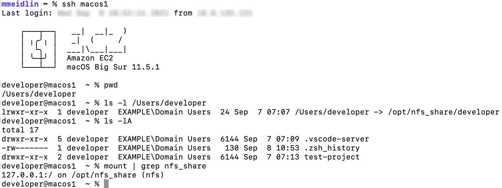
When you connect via the preceding command, your local machine first establishes an SSH connection to the bastion host which authorizes the request against the key we just stored in Active Directory. Upon success, the bastion host forwards the connection to the macos1 instance, which again authorizes against Active Directory and launches a  terminal session upon success. The following figure illustrates the login with the macos1 instances, showcasing both the integration with AD (EXAMPLE\Domain Users group membership) as well as with the EFS share, which is mounted at /opt/nfsshare and symlinked to the developer’s home directory.

Screenshot from a terminal window after logging into the macos1 instance. Instructions for doing this are included in the blog text.

Likewise, you can create folders and files in the developer’s home directory such as the test-project folder depicted in the screenshot.

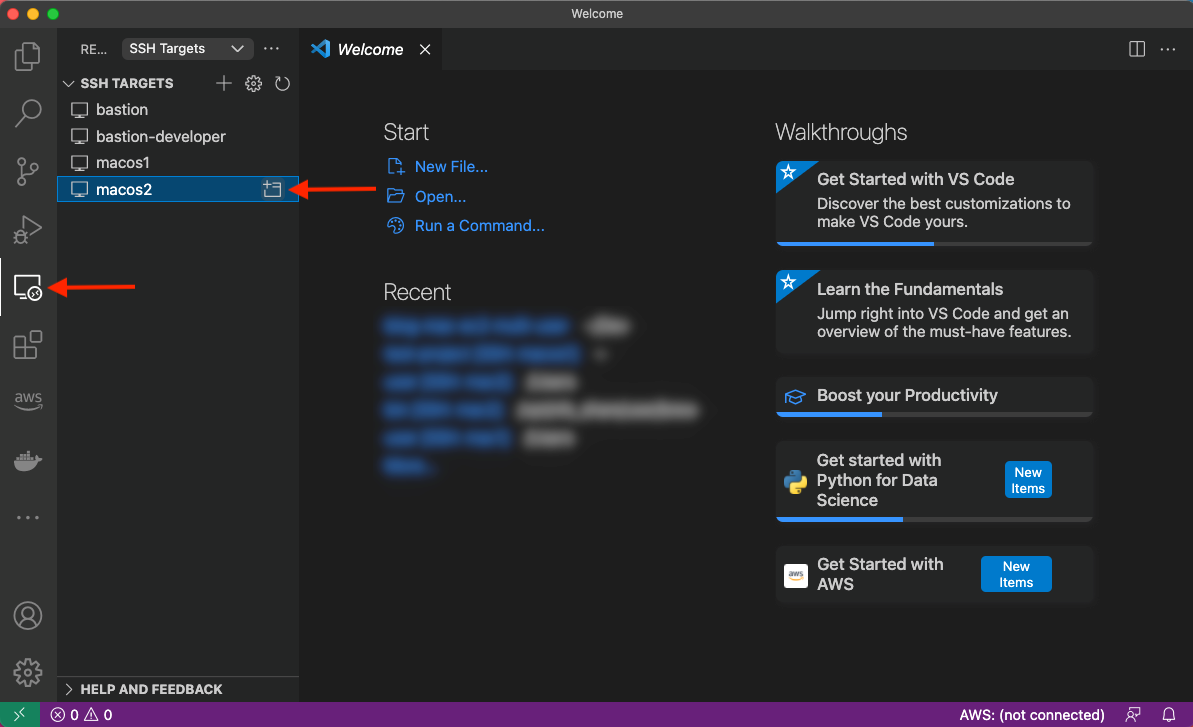
Lastly, let’s utilize VS Code’s remote plugin and connect to the other macos2 instance. Select the Remote Explorer on the left-hand pane and click to open the macos2 host as shown in the following screenshot:

Screenshot depicting how to connect to the macos2 instance using the VSCode Remote SSH extension.

A new window will be opened with the context of the remote server, as shown in the next figure. As you can see, we have access to the same files seen previously on the macos1 host.

Screenshot showing VSCode UI once connected to the macos2 instance.

Cleanup

From the repository root, run the provided destroy.sh script in order to destroy all resources created by CloudFormation, specifying the stack name as input parameter:

./destroy.sh ec2-mac-remote-dev-env

Check the CloudFormation Console to confirm that the stack and its resources are properly deleted.

Lastly, in the EC2 Console, release the dedicated Mac Hosts that you allocated in the beginning. Notice that this is only possible 24 hours after allocation.

Summary

This post has shown how EC2 Mac instances can be set up as remote development environments, thereby allowing developers to create software for Apple platforms regardless of their local hardware and software setup. Aside from increased flexibility and maintainability, this setup also saves cost because multiple developers can work interactively with the same EC2 Mac instance. We have rolled out an architecture that integrates EC2 Mac instances with AWS Directory Services for centralized user and access management as well as Amazon EFS to store developer home directories in a durable and highly available manner. This has resulted in an architecture where instances can easily be added, removed, or updated without affecting developer workflow. Now, irrespective of your client machine, you are all set to start coding with your local editor while leveraging EC2 Mac instances in the AWS Cloud to provide you with a macOS environment! To get started and learn more about EC2 Mac instances, please visit the product page.

Field Notes: Building On-Demand Disaster Recovery for IBM DB2 on AWS

Post Syndicated from João Bozelli original https://aws.amazon.com/blogs/architecture/field-notes-building-on-demand-disaster-recovery-for-ibm-db2-on-aws/

With the increased adoption of critical applications running in the cloud, customers often find themselves revisiting traditional strategies that were adopted for on-premises workloads. When it comes to IBM DB2, one of the first decisions to make is to decide what backup and restore method will be used.

In this blog post, we will show you how IT architects, database administrators, and cloud administrators can use AWS services such as Amazon Machine Images (AMIs) and Amazon Simple Storage Service (Amazon S3) to build on-demand disaster recovery. This is useful for organizations who are flexible in their Recovery Time Objective (RTO) to reduce cost by only provisioning the target environment when needed.

Architecture overview

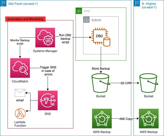
Figure 1. Architecture of AWS services used in this blog post

Figure 1 shows the Amazon Elastic Compute Cloud (Amazon EC2) instance running the DB2 database in the primary Region (São Paulo, in this example) and performing backups to Amazon S3 by a script initiated by AWS Systems Manager. The backups in Amazon S3 are then replicated to the secondary Region (N. Virginia, in this example) by the S3 Cross-Region Replication (CRR) feature of Amazon S3.

AWS Backup provides automation by performing the AMI copy and in a similar fashion to the database backups, the AMIs are copied to the secondary Region as well. You can further enhance the backup mechanism by activating monitoring through Amazon CloudWatch and using Amazon Simple Notification Service (Amazon SNS) to send out alerts in the event of failures. The architectural considerations will be outlined in detail.

Configuring IBM DB2 native data backup to Amazon S3

Database backups are stored in Amazon S3, which replicates the backups inside a Region by default and can be replicated to another Region using CRR. Since version 11.1, IBM DB2 running on Linux natively supports data backups to Amazon S3. To create this architecture, follow these steps:

  1. Log in to the Linux server and create a PKCS keystore to store the key and create a secret access key that will be used to transfer the data to Amazon S3. The remote storage credentials will be stored in this keystore.
cd /db2/db2<sid>/
mkdir .keystore
gsk8capicmd_64 -keydb -create -db "/db2/db2<sid>/.keystore/db6-s3.p12" -pw "<password>" -type pkcs12 -stash
  1. Configure IBM DB2 to use the keystore with the KEYSTORE_LOCATION and KEYSTORE_TYPE parameters.
db2 "update dbm cfg using keystore_location /db2/db2<sid>/.keystore/db6-s3.p12 keystore_type pkcs12"
  1. Validate that the parameters were successfully updated.
db2 get dbm cfg |grep -i KEYSTORE
 Keystore type                           (KEYSTORE_TYPE) = PKCS12
 Keystore location                   (KEYSTORE_LOCATION) = /db2/db2<sid>/.keystore/db6-s3.p12
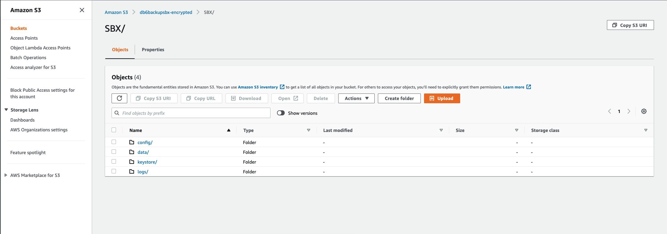
  1. Create an S3 bucket in the same Region where your EC2 instance running the IBM DB2 database is located. Ensure that all security best practices are followed for the creation of the bucket. This bucket will store the backup images. You can create different folders to store different objects. For example, you can store the configuration files in a different path, or separate backups from different IBM DB2 instances by folders inside one bucket.

Figure 2. Example bucket for storing backups

In this example, the primary folder for this database is SBX. The folder data will store the data backups, the folder config will store the configuration parameters, the folder keystore will store the backup of the keystore, and the folder logs will store the database logs.

  1. A user with programmatic access is required, because the only method of authentication available is using an access key (access key ID and secret access key). Create the user with the proper S3 permissions (the best practice is to use the principle of least privilege) and note the access key ID and secret access key. Then, create an IBM DB2 storage access alias using the following syntax:
db2 "catalog storage access alias <alias_name> vendor S3 server <S3 endpoint> user '<access_key>' password '<secret_access_key>' container '<bucket_name>'"
  1. Set the staging path to where the backups will be stored before moving to Amazon S3. This is done by defining the environment variable. Ensure this is set to avoid that the backup is written to an unwanted path.
db2set DB2_OBJECT_STORAGE_LOCAL_STAGING_PATH=/backup/staging/data
  1. To validate if variable was properly set, check that the IBM DB2 variable DB2_OBJECT_STORAGE_LOCAL_STAGING_PATH is set as follows:
db2set |grep -i STAGING

DB2_OBJECT_STORAGE_LOCAL_STAGING_PATH=/backup/staging/data
  1. Initiate the database backup either by the following command or with your backup script.

Note: make sure that the target is DB2REMOTE as follows:

db2 BACKUP DATABASE <instance> TO DB2REMOTE://<alias>//<path>/<additional path> compress without prompting

While the backup is running, you will see data being stored in the staging directory (for this example: /backup/staging/data), and then uploaded to Amazon S3.

The backup script can be integrated with AWS Systems Manager maintenance windows to run on schedule to allow control and visibility. When combined with Amazon SNS, you can send out notifications in case of success, failures, or both.

Set log and DB2 config backup to Amazon S3

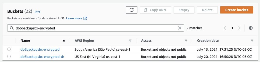
There are different options when it comes to storing the database logs into Amazon S3. In this example, we’re using a very simple script initiated by AWS Systems Manager to sync the logs from the staging disk to Amazon S3. This, combined with CRR, increases the durability of the backup by replicating the logs to another Region of your choice. The same backup method for the logs is applied to the IBM DB2 configuration files (parameters and variables) and the keystore. Figure 3 shows the CRR configured on the target bucket, which is then automatically replicating the data to a secondary Region (us-east-1).

Figure 3. Example buckets for IBM DB2 backup and disaster recovery, respectively

Figure 4. Amazon S3 Replication rules configured from sa-east-1 to us-east-1 (São Paulo to N. Virginia)

Figure 5. IBM DB2 logs backed up in São Paulo (sa-east-1) and replicated to N. Virginia (us-east-1)

Amazon S3 Lifecycle policy

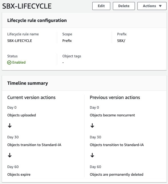
For this use case, we have defined a lifecycle policy to maintain the objects (full and log backups) stored as Amazon S3 Standard for 30 days, afterwards they will be moved from Amazon S3 Standard to Amazon S3 Standard-IA. After 30 days, any objects stored as Amazon S3 Standard-IA will be deleted. When used in the context of a database, this allows you to automatically manage the lifecycle of your backups. If you have compliance needs to store specific backups with longer retention times, you can backup to a separate folder (prefix) with a different lifecycle rule.

Figure 6. Amazon S3 Lifecycle policy configure for buckets in São Paulo (sa-east-1) and N. Virginia (us-east-1)

AMI to aid with automation

Up to this point, this blog post has covered how you can manage the backups for a better Recovery Point Objective (RPO). However, let’s consider what happens in case of a disaster or if you have issues with the server running the IBM DB2 database. The Recovery Time Objective (RTO) will be higher because you will have to launch an EC2 instance, prepare the server, install the IBM DB2 database, and restore the full data and log backups.

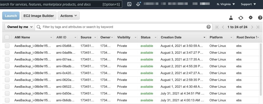
To reduce your RTO, we recommend using automated AMI backups for your EC2 instance. AWS Backup helps you generate automated AMIs based on tags and resource IDs. AWS Backup can ship the AMI backup generated from your instance to another Region, for a multi-Region disaster recovery strategy.

In this example, we have created an AWS Backup plan to run twice a day and to ship a copy of the AMI from São Paulo (sa-east-1) to N. Virginia (sa-east-1).

Figure 7. Automated AMIs copied from São Paulo (sa-east-1) to N. Virginia (us-east-1) by AWS Backup

Performance considerations

It is important to discuss the factors that impact overall backup and restore performance, and ultimately the RTO.

We recommend using VPC endpoints to ensure that the traffic from your EC2 to Amazon S3 does not traverse the internet, and to provide improved throughput for data upload. Another important factor is the type of EBS volumes used for storing the IBM DB2 data files. In this example, to cover a 170 GB database, the disk used was GP2 not striped in Logical Volume Manager (LVM). Because the degree of parallelism (number of tablespaces read in parallel by the IBM DB2 backup process) can increase CPU usage, caution is warranted when running online backups so as not to cause too much overhead on your database server. When considering optimization for EBS volumes, note the maximum throughput and IOPS that can be reached by instance type.

A test was run using AWS Command Line Interface to sync 100 GB of logs (100 files of 1 GB) from Amazon S3 to the newly created instance. It took 16 minutes. The amount of logs will vary depending on the backup schedule implemented. The Amazon S3 costs will vary depending on the lifecycle policies implemented. For further details, refer to Amazon S3 pricing.

Results

In our tests, the backup time for a 170 GB database took 38 minutes, with a restore time of 14 minutes.

The restore time can vary depending on the backup size, the amount of logs to roll forward, and disk type (mentioned previously in the Performance considerations section).

With the results of this test, the RTO was the restore time plus the time taken to launch the new server based off the AMI backup taken.

Table 1. Recovery test
Disk Type DB Size Instance Type (Backup) Parallel Channels (Backup) Backup Time Instance Type (Restore) Parallel Channels (Restore) Restore Time
GP2 170 GB m5.4xlarge 12 38 Minutes m5.4xlarge 12 14 Minutes

Conclusion

To summarize, in this blog post we described how to configure IBM DB2 backups to Amazon S3, to build an on-demand strategy for backup and disaster recovery. By following these architecture design principles, you will continue to develop resilient business continuity. Let us know if you have any comments or questions. We value your feedback!

Field Notes provides hands-on technical guidance from AWS Solutions Architects, consultants, and technical account managers, based on their experiences in the field solving real-world business problems for customers.

Accelo uses Amazon QuickSight to accelerate time to value in delivering embedded analytics to professional services businesses

Post Syndicated from Mahlon Duke original https://aws.amazon.com/blogs/big-data/accelo-uses-amazon-quicksight-to-accelerate-time-to-value-in-delivering-embedded-analytics-to-professional-services-businesses/

This is a guest post by Accelo. In their own words, “Accelo is the leading cloud-based platform for managing client work, from prospect to payment, for professional services companies. Each month, tens of thousands of Accelo users across 43 countries create more than 3 million activities, log 1.2 million hours of work, and generate over $140 million in invoices.”

Imagine driving a car with a blacked-out windshield. It sounds terrifying, but it’s the way things are for most small businesses. While they look into the rear-view mirror to see where they’ve been, they lack visibility into what’s ahead of them. The lack of real-time data and reliable forecasts leaves critical decisions like investment, hiring, and resourcing to “gut feel.” An industry survey conducted by Accelo shows 67% of senior leaders don’t have visibility into team utilization, and 54% of them can’t track client project budgets, much less profitability.

Professional services businesses generate most of their revenue directly from billable work they do for clients every day. Because no two clients, projects, or team members are the same, real-time and actionable insight is paramount to ensure happy clients and a successful, profitable business. A big part of the problem is that many businesses are trying to manage their client work with a cocktail of different, disconnected systems. No wonder KPMG found that 56% of CEOs have little confidence in the integrity of the data they’re using for decision-making.

Accelo’s mission is to solve this problem by giving businesses an integrated system to manage all their client work, from prospect to payment. By combining what have historically been disparate parts of the business—CRM, sales, project management, time tracking, client support, and billing—Accelo becomes the single source of truth for your business’s most important data.

Even with a trustworthy, automated and integrated system, decision makers still need to harness the data so they see what’s in front of them and can anticipate for the future. Accelo devoted all our resources and expertise to building a complete client work management platform, made up of essential products to achieve the greatest profitability. We recognized that in order to make the platform most effective, users needed to be empowered with the strongest analytics and actionable insights for strategic decision making. This drove us to seek out a leading BI solution that could seamlessly integrate with our platform and create the greatest user experience. Our objective was to ensure that Accelo users had access to the best BI tool without requiring them to spend more of their valuable time learning yet another tool – not to mention another login. We needed a powerful embedded analytics solution.

We evaluated dozens of leading BI and embedded reporting solutions, and Amazon QuickSight was the clear winner. In this post, we discuss why, and how QuickSight accelerated our time to value in delivering embedded analytics to our users.

Data drives insights

Even today, many organizations track their work manually. They extract data from different systems that don’t talk to each other, and manually manipulate it in spreadsheets, which wastes time and introduces the kinds of data integrity problems that cause CEOs to lose their confidence. As companies grow, these manual and error-prone approaches don’t scale with them, and the sheer level of effort required to keep data up to date can easily result in leaders just giving up.

With this in mind, Accelo’s embedded analytics solution was built from the ground up to grow with us and with our users. As a part of the AWS family, QuickSight eliminated one of the biggest hurdles for embedded analytics through its SPICE storage system. SPICE enables us to create unlimited, purpose-built datasets that are hosted in Amazon’s dynamic storage infrastructure. These smaller datasets load more quickly than your typical monolithic database, and can be updated as often as we need, all at an affordable per-gigabyte rate. This allows us to provide real-time analytics to our users swiftly, accurately, and economically.

“Being able to rely on Accelo to tell us everything about our projects saves us a lot of time, instead of having to go in and download a lot of information to create a spreadsheet to do any kind of analysis,” says Katherine Jonelis, Director of Operations, MHA Consulting. “My boss loves the dashboards. He loves just being able to look at that and instantly know, ‘Here’s where we are.’”

In addition to powering analytics for our users, QuickSight also helps our internal teams identify and track vital KPIs, which historically has been done via third-party apps. These metrics can cover anything, from calculating the effective billable rate across hundreds of projects and thousands of time entries, to determining how much time is left for the team to finish their tasks profitably and on budget. Because the reports are embedded directly in Accelo, which already houses all the data, it was easy for our team to adapt to the new reports and require minimal training.

Integrated vs. embedded

One of the most important factors in our evaluation of BI platforms was the time to value. We asked ourselves two questions: How long would it take to have the solution up and running, and how long would it take for our users to see value from it?

While there are plenty of powerful third-party, integrated BI products out there, they often require a complete integration, adding authentication and configuration on top of basic data extraction and transformations. This makes them an unattractive option, especially in an increasingly security-focused landscape. Meanwhile, most of the embedded products we evaluated required a time to launch that numbered in the months—spending time on infrastructure, data sources, and more. And that’s without considering the infrastructure and engineering costs of ongoing maintenance. One key benefit that propels QuickSight above other products is that it allowed us to reduce that setup time from months to weeks, and completely eliminated any configuration work for the end-user. This is possible thanks to built-in tools like native connections for AWS data sources, row-level security for datasets, and a simple user provisioning process.

Developer hours can be expensive, and are always in high demand. Even in a responsive and agile development environment like Accelo’s, development work still requires lead time before it can be scheduled and completed. Engineering resources are also finite—if they’re working on one thing today, something else is probably going into the backlog. QuickSight enables us to eliminate this bottleneck by shifting the task of managing these analytics from developers to data analysts. We used QuickSight to easily create datasets and reports, and placed a simple API call to embed them for our clients so they can start using them instantly. Now we’re able to quickly respond to our users’ ever-changing needs without requiring developers. That further improves the speed and quality of our data by using both the analysts’ general expertise with data visualization and their unique knowledge of Accelo’s schema. Today, all of Accelo’s reports are created and deployed through QuickSight. We’re able to accommodate dozens of custom requests each month for improvements—major and minor—without ever needing to involve a developer.

Implementation and training were also key considerations during our evaluation. Our customers are busy running their businesses. The last thing they want is to get trained on a new tool, not to mention the typically high cost associated with implementation. As a turnkey solution that requires no configuration and minimal education, QuickSight was the clear winner.

Delivering value in an agile environment

It’s no secret that employees dislike timesheets and would rather spend time working with their clients. For many services companies, logged time is how they bill their clients and get paid. Therefore, it’s vital that employees log all their hours. To make that process as painless as possible, Accelo offers several tools that minimize the amount of work it takes an employee to log their time. For example, the Auto Scheduling tool automatically builds out employees’ schedules based on the work they’re assigned, and logs their time with a single click. Inevitably, however, someone always forgets to log their time, leading to lost revenue.

To address this issue, Accelo built the Missing Time report, which pulls hundreds of thousands of time entries, complex work schedules, and even holiday and PTO time together to offer answers to these questions: Who hasn’t logged their time? How much time is missing? And from what time period?

Every business needs to know whether they’re profitable. Professional services businesses are unique in that profitability is tied directly to their individual clients and the relationships with them. Some clients may generate high revenues but require so much extra maintenance that they become unprofitable. On the other hand, low-profile clients that don’t require a lot of attention can significantly contribute to the business’s bottom line. By having all the client data under one roof, these centralized and embedded reports can provide visibility into your budgets, time entries, work status, and team utilization. This makes it possible to make real-time, data-driven actions without having to spend all day to get the data.

Summary

Clean and holistic data fosters deep insights that can lead to higher margins and profits. We’re excited to partner with AWS and QuickSight to provide professional services businesses with real-time insights into their operations so they can become truly data driven, effortlessly. Learn more about Accelo, and Amazon QuickSight Embedded Analytics!


About the Authors

Mahlon Duke, Accelo Product Manager of BI and Data.

Geoff McQueen, Accelo Founder and CEO.

Publishing messages in batch to Amazon SNS topics

Post Syndicated from Talia Nassi original https://aws.amazon.com/blogs/compute/publishing-messages-in-batch-to-amazon-sns-topics/

This post is written by Heeki Park (Principal Solutions Architect, Serverless Specialist), Marc Pinaud (Senior Product Manager, Amazon SNS), Amir Eldesoky (Software Development Engineer, Amazon SNS), Jack Li (Software Development Engineer, Amazon SNS), and William Nguyen (Software Development Engineer, Amazon SNS).

Today, we are announcing the ability for AWS customers to publish messages in batch to Amazon SNS topics. Until now, you were only able to publish one message to an SNS topic per Publish API request. With the new PublishBatch API, you can send up to 10 messages at a time in a single API request. This reduces cost for API requests by up to 90%, as you need fewer API requests to publish the same number of messages.

Introducing the PublishBatch API

Consider a log processing application where you process system logs and have different requirements for downstream processing. For example, you may want to do inference on
incoming log data, populate an operational Amazon OpenSearch Service environment, and store log data in an enterprise data lake.

Systems send log data to a standard SNS topic, and Amazon SQS queues and Amazon Kinesis Data Firehose are configured as subscribers. An AWS Lambda function subscribes to the first SQS queue and uses machine learning models to perform inference to detect security incidents or system access anomalies. A Lambda function subscribes to the second SQS queue and emits those log entries to an Amazon OpenSearch Service cluster. The workload uses Kibana dashboards to visualize log data. An Amazon Kinesis Data Firehose delivery stream subscribes to the SNS topic and archives all log data into Amazon S3. This allows data scientists to conduct further investigation and research on those logs.

To do this, the following Java code publishes a set of log messages. In this code, you construct a publish request for a single message to an SNS topic and submit that request via the publish() method:

// tab 1: standard publish example
private static AmazonSNS snsClient;
private static final String MESSAGE_PAYLOAD = " 192.168.1.100 - - [28/Oct/2021:10:27:10 -0500] "GET /index.html HTTP/1.1" 200 3395";

PublishRequest request = new PublishRequest()
    .withTopicArn(topicArn)
    .withMessage(MESSAGE_PAYLOAD);
PublishResult response = snsClient.publish(request);

// tab 2: fifo publish example
private static AmazonSNS snsClient;
private static final String MESSAGE_PAYLOAD = " 192.168.1.100 - - [28/Oct/2021:10:27:10 -0500] "GET /index.html HTTP/1.1" 200 3395";
private static final String MESSAGE_FIFO_GROUP = "server1234";

PublishRequest request = new PublishRequest()
    .withTopicArn(topicArn)
    .withMessage(MESSAGE_PAYLOAD)
    .withMessageGroupId(MESSAGE_FIFO_GROUP)
    .withMessageDeduplicationId(UUID.randomUUID().toString());
PublishResult response = snsClient.publish(request);

If you extended the example above and had 10 log lines that each needed to be published as a message, you would have to write code to construct 10 publish requests, and subsequently submit each of those requests via the publish() method.

With the new ability to publish batch messages, you write the following new code. In the code below, you construct a list of publish entries first, then create a single publish batch request, and subsequently submit that batch request via the new publishBatch() method. In the code below, you use a sample helper method getLoggingPayload(i) to get the appropriate payload for the message, which you can replace with your own business logic.

// tab 1: standard publish example
private static final String MESSAGE_BATCH_ID_PREFIX = "server1234-batch-id-";

List<PublishBatchRequestEntry> entries = IntStream.range(0, 10)
.mapToObj(i -> {
new PublishBatchRequestEntry()
.withId(MESSAGE_BATCH_ID_PREFIX + i)
.withMessage(getLoggingPayload(i));
})
.collect(Collectors.toList());
PublishBatchRequest request = new PublishBatchRequest()
.withTopicArn(topicArn)
.withPublishBatchRequestEntries(entries);
PublishBatchResult response = snsClient.publishBatch(request);

// tab 2: fifo publish example
private static final String MESSAGE_BATCH_ID_PREFIX = "server1234-batch-id-";
private static final String MESSAGE_FIFO_GROUP = "server1234";


List<PublishBatchRequestEntry> entries = IntStream.range(0, 10)
.mapToObj(i -> {
new PublishBatchRequestEntry()
.withId(MESSAGE_BATCH_ID_PREFIX + i)
.withMessage(getLoggingPayload(i))
.withMessageGroupId(MESSAGE_FIFO_GROUP)
.withMessageDeduplicationId(UUID.randomUUID().toString());
})
.collect(Collectors.toList());
PublishBatchRequest request = new PublishBatchRequest()
.withTopicArn(topicArn)
.withPublishBatchRequestEntries(entries);
PublishBatchResult response = snsClient.publishBatch(request);

In the list of publish requests, the application must assign a unique batch ID (up to 80 characters) to each publish request within that batch. When the SNS service successfully receives a message, the SNS service assigns a unique message ID and returns that message ID in the response object.

If publishing to a FIFO topic, the SNS service additionally returns a sequence number in the response. When publishing a batch of messages, the PublishBatchResult object returns a list of response objects for successful and failed messages. If you iterate through the list of response objects for successful messages, you might see the following:

// tab 1: standard publish output
{
"Id": "server1234-batch-id-0",
"MessageId": "fcaef5b3-e9e3-5c9e-b761-ac46c4a779bb",
...
}

// tab 2: fifo publish output
{
"Id": "server1234-batch-id-0",
"MessageId": "fcaef5b3-e9e3-5c9e-b761-ac46c4a779bb",
"SequenceNumber": "10000000000000003000",
...
}

When receiving the message from SNS in the SQS queue, the application reads the following message:

// tab 1: standard publish output
{
"Type" : "Notification",
"MessageId" : "fcaef5b3-e9e3-5c9e-b761-ac46c4a779bb",
"TopicArn" : "arn:aws:sns:us-east-1:112233445566:publishBatchTopic",
"Message" : "payload-0",
"Timestamp" : "2021-10-28T22:58:12.862Z",
"UnsubscribeURL" : "http://sns.us-east-1.amazon.com/?Action=Unsubscribe&SubscriptionArn=arn:aws:sns:us-east-1:112233445566:publishBatchTopic:ff78260a-0953-4b60-9c2c-122ebcb5fc96"
}

// tab 2: fifo publish output
{
"Type" : "Notification",
"MessageId" : "fcaef5b3-e9e3-5c9e-b761-ac46c4a779bb",
"SequenceNumber" : "10000000000000003000",
"TopicArn" : "arn:aws:sns:us-east-1:112233445566:publishBatchTopic",
"Message" : "payload-0",
"Timestamp" : "2021-10-28T22:58:12.862Z",
"UnsubscribeURL" : "http://sns.us-east-1.amazon.com/?Action=Unsubscribe&SubscriptionArn=arn:aws:sns:us-east-1:112233445566:publishBatchTopic.fifo:ff78260a-0953-4b60-9c2c-122ebcb5fc96"
}

In the standard publish example, the MessageId of fcaef5b3-e9e3-5c9e-b761-ac46c4a779bb is propagated down to the message in SQS. In the FIFO publish example, the SequenceNumber of 10000000000000003000 is also propagated down to the message in SQS.

Handling errors and quotas

When publishing messages in batch, the application must handle errors that may have occurred during the publish batch request. Errors can occur at two different levels. The first is when publishing the batch request to the SNS topic. For example, if the application does not specify a unique message batch ID, it fails with the following error:

com.amazonaws.services.sns.model.BatchEntryIdsNotDistinctException: Two or more batch entries in the request have the same Id. (Service: AmazonSNS; Status Code: 400; Error Code: BatchEntryIdsNotDistinct; Request ID: 44cdac03-eeac-5760-9264-f5f99f4914ad; Proxy: null)

The second is within the batch request at the message level. The application must inspect the returned PublishBatchResult object by iterating through successful and failed responses:

PublishBatchResult publishBatchResult = snsClient.publishBatch(request);
publishBatchResult.getSuccessful().forEach(entry -> {
System.out.println(entry.toString());
});

publishBatchResult.getFailed().forEach(entry -> {
System.out.println(entry.toString());
});

With respect to quotas, the overall message throughput for an SNS topic remains the same. For example, in US East (N. Virginia), standard topics support up to 30,000 messages per second. Before this feature, 30,000 messages also meant 30,000 API requests per second. Because SNS now supports up to 10 messages per request, you can publish the same number of messages using only 3,000 API requests. With FIFO topics, the message throughput remains the same at 300 messages per second, but you can now send that volume of messages using only 30 API requests, thus reducing your messaging costs with SNS.

Conclusion

SNS now supports the ability to publish up to 10 messages in a single API request, reducing costs for publishing messages into SNS. Your applications can validate the publish status of each of the messages sent in the batch and handle failed publish requests accordingly. Message throughput to SNS topics remains the same for both standard and FIFO topics.

Learn more about this ability in the SNS Developer Guide.
Learn more about the details of the API request in the SNS API reference.
Learn more about SNS quotas.

For more serverless learning resources, visit Serverless Land.

[$] What to do in response to a kernel warning

Post Syndicated from original https://lwn.net/Articles/876209/rss

The kernel provides a number of macros internally to allow code to generate
warnings when something goes wrong. It does not, however, provide a lot of
guidance regarding what should happen when a warning is issued. Alexander
Popov recently posted a
patch series
adding an option for the system’s response to warnings;
that series seems unlikely to be applied in anything close to its current
form, but it did succeed in provoking a discussion on how warnings should
be handled.

Design and build a Data Vault model in Amazon Redshift from a transactional database

Post Syndicated from George Komninos original https://aws.amazon.com/blogs/big-data/design-and-build-a-data-vault-model-in-amazon-redshift-from-a-transactional-database/

Building a highly performant data model for an enterprise data warehouse (EDW) has historically involved significant design, development, administration, and operational effort. Furthermore, the data model must be agile and adaptable to change while handling the largest volumes of data efficiently.

Data Vault is a methodology for delivering project design and implementation to accelerate the build of data warehouse projects. Within the overall methodology, the Data Vault 2.0 data modeling standards are popular and widely used within the industry because they emphasize the business keys and their associations within the delivery of business processes. Data Vault facilitates the rapid build of data models via the following:

  • Pattern-based entities each with a well-defined purpose
  • Data silos are removed because data is represented in source system independent structures
  • Data can be loaded in parallel with minimum dependencies
  • Historized data is stored at its lowest level of granularity
  • Flexible business rules can be applied independently of the loading of the data
  • New data sources can be added with no impact on the existing model.

We always recommend working backwards from the business requirements to choose the most suitable data modelling pattern to use; there are times where Data Vault will not be the best choice for your enterprise data warehouse and another modelling pattern will be more suitable.

In this post, we demonstrate how to implement a Data Vault model in Amazon Redshift and query it efficiently by using the latest Amazon Redshift features, such as separation of compute from storage, seamless data sharing, automatic table optimizations, and materialized views.

Data Vault data modeling overview

A data warehouse platform built using Data Vault typically has the following architecture:

The architecture consists of four layers:

  • Staging – Contains a copy of the latest changes to data from the source systems. This layer doesn’t hold history and, during its population, you can apply several transformations to the staged data, including data type changes or resizing, character set conversion, and the addition of meta-data columns to support later processing.
  • Raw Data Vault – Holds the historized copy of all of the data from multiple source systems. No filters or business transformations have occurred at this point except for storing the data in source-system independent targets.
  • Business Data Vault – An optional delivery, but is very often built. It contains business calculations and de-normalizations with the sole purpose of improving the speed and simplicity of access within the consumption layer, which is called the Information Mart layer.
  • Information Mart Layer – Where data is most commonly accessed by consumers, for example reporting dashboards or extracts. You can build multiple marts from the one Data Vault Integration Layer, and the most common data modeling choice for these marts is Star/Kimball schemas.

Convert a Third Normal Form transactional schema to a Data Vault schema

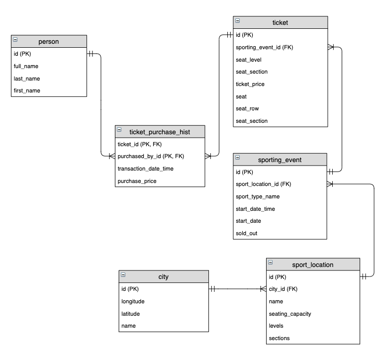
The following entity relationship diagram is a standard implementation of a transactional model that a sports ticket selling service could use:

The main entities within the schema are sporting events, customers, and tickets. A customer is a person, and a person can purchase one or multiple tickets for a sporting event. This business event is captured by the Ticket Purchase History intersection entity above. Finally, a sporting event has many tickets available to purchase and is staged within a single city.

To convert this source model to a Data Vault model, we start to identify the business keys, their descriptive attributes, and the business transactions. The three main entity types in the Raw Data Vault model are as follows:

  • Hubs – A collection of Business Keys discovered for each business entity.
  • Links – Business transactions within the process being modelled. This is always between two or more business keys (hubs) and recorded at a point in time.
  • Satellites – Historized reference data about either the business key (Hub) or business transaction (link).

The following example solution represents some of the sporting event entities when converted into the preceeding Raw Data Vault objects.

Hub entities

The hub is the definitive list of business keys loaded into the Raw Data Vault layer from all of the source systems. A business key is used to uniquely identify a business entity and is never duplicated. In our example, the source system has assigned a surrogate key field called Id to represent the Business Key, so this is stored in a column on the Hub called sport_event_id. Some common additional columns on hubs include the Load DateTimeStamp which records the date and time the business key was first discovered, and the Record Source which records the name of the source system where this business key was first loaded. Although, you don’t have to create a surrogate type (hash or sequence) for the primary key column, it is very common in Data Vault to hash the business key, so our example does this. Amazon Redshift supports multiple cryptographic hash functions like MD5, FNV, SHA1, and SHA2, which you can choose to generate your primary key column. See the following code :

create table raw_data_vault.hub_sport_event 
(
  sport_event_pk  varchar(32) not null     
 ,sport_event_id  integer     not null
 ,load_dts        timestamp   not null       
 ,record_source   varchar(10) not null      
);

Note the following:

  • The preceeding code assumes the MD5 hashing algorithm is used. If using FNV_HASH, the datatype will be Bigint.
  • The Id column is the business key from the source feed. It’s passed into the hashing function for the _PK column.
  • In our example, there is only a single value for the business key. If a compound key is required, then more than one column can be added.
  • Load_DTS is populated via the staging schema or extract, transform, and load (ETL) code.
  • Record_Source is populated via the staging schema or ETL code.

Link entities

The link object is the occurrence of two or more business keys undertaking a business transaction, for example purchasing a ticket for a sporting event. Each of the business keys is mastered in their respective hubs, and a primary key is generated for the link comprising all of the business keys (typically separated by a delimiter field like ‘^’). As with hubs, some common additional columns are added to links, including the Load DateTimeStamp which records the date and time the transaction was first discovered, and the Record Source which records the name of the source system where this transaction was first loaded. See the following code:

create table raw_data_vault.lnk_ticket_sport_event 
(
  ticket_sport_event_pk varchar(32)  not null    
 ,ticket_fk             varchar(32)  not null   
 ,sport_event_fk        varchar(32)  not null   
 ,load_dts              timestamp    not null   
 ,record_source         varchar(10)  not null   
);

Note the following:

  • The code assumes that the MD5 hashing algorithm is used. The _PK column is hashed values of concatenated ticket and sporting event business keys from the source data feed, for example MD5(ticket_id||'^'||sporting_event_id)
  • The two _FK columns are foreign keys linked to the primary key of the respective hubs.
  • Load_DTS is populated via the staging schema or ETL code.
  • Record_Source is populated via the staging schema or ETL code.

Satellite entities

The history of data about the hub or link is stored in the satellite object. The Load DateTimeStamp is part of the compound key of the satellite along with the primary key of either the hub or link because data can change over time. There are choices within the Data Vault standards for how to store satellite data from multiple sources. A common approach is to append the name of the feed to the satellite name. This lets a single hub contain reference data from more than one source system, and for new sources to be added without impact to the existing design. See the following code:

create table raw_data_vault.sat_sport_event 
(
  sport_event_pk    varchar(32) not null     
 ,load_dts          timestamp   not null  
 ,sport_type_name   varchar(50)
 ,start_datetime    timestamp
 ,sold_out          boolean     
 ,record_source     varchar(10) not null 
 ,hash_diff         varchar(32) not null 
);

Note the following:

  • The sport_event_pk value is inherited from the hub.
  • The compound key is the sport_event_pk and load_dts columns. This allows history to be maintained.
  • The business attributes are typically optional.
  • Load_DTS is populated via the staging schema or ETL code.
  • Record_Source is populated via the staging schema or ETL code.
  • Hash_Diff is a Data Vault technique to simplify the identification of data changes within satellites. The business attribute values are concatenated and hashed with your algorithm of choice. Then, during the ETL processing, only the two hash values (one on the source record and one on the latest dated satellite record) should be compared.

Converted Data Vault Model

If we take the preceding three Data Vault entity types above, we can convert the source data model into a Data Vault data model as follows:

The Business Data Vault contains business-centric calculations and performance de-normalizations that are read by the Information Marts. Some of the object types that are created in the Business Vault layer include the following:

  • PIT (point in time) tables – You can store data in more than one satellite for a single hub, each with a different Load DateTimeStamp depending on when the data was loaded. A PIT table simplifies access to all of this data by creating a table or materialized view to present a single row with all of the relevant data to hand. The compound key of a PIT table is the primary key from the hub, plus a snapshot date or snapshot date and time for the frequency of the population. Once a day is the most popular, but equally the frequency could be every 15 minutes or once a month.
  • Bridge tables – Similar to PIT tables, bridge tables take the data from more than one link or link satellite and again de-normalize into a single row. This single row view makes accessing complex datasets over multiple tables from the Raw Data Vault much more straightforward and performant. Like a PIT table, the bridge table can be either a table or materialized view.
  • KPI tables – The pre-computed business rules calculate KPIs and store them in dedicated tables.
  • Type 2 tables –You can apply additional processing in the Business Data Vault to calculate Type 2 like time periods because the data in the Raw Data Vault follows an insert only pattern.

The architecture of Amazon Redshift allows flexibility in the design of the Data Vault platform by using the capabilities of the Amazon Redshift RA3 instance type to separate the compute resources from the data storage layer and the seamless ability to share data between different Amazon Redshift clusters. This flexibility allows highly performant and cost-effective Data Vault platforms to be built. For example, the Staging and Raw Data Vault Layers are populated 24-hours-a-day in micro batches by one Amazon Redshift cluster, the Business Data Vault layer can be built one-time-a-day and paused to save costs when completed, and any number of consumer Amazon Redshift clusters can access the results. Depending on the processing complexity of each layer, Amazon Redshift supports independently scaling the compute capacity required at each stage.

All of the underlying tables in Raw Data Vault can be loaded simultaneously. This makes great use of the massively parallel processing architecture in Amazon Redshift. For our business model, it makes sense to create a Business Data Vault layer, which can be read by an Information Mart to perform dimensional analysis on ticket sales. It can give us insights on the top home teams in fan attendance and how that correlates with specific sport locations or cities. Running these queries involves joining multiple tables. It’s important to design an optimal Business Data Vault layer to avoid excessive joins for deriving these insights.

For example, to get the number of tickets per city for June 2021, the SQL looks like the following code:

SELECT name,count(lpt.ticket_fk) as tickets_sold
FROM lnk_person_ticket lpt
  JOIN lnk_ticket_sport_event ltse on lpt.ticket_fk = ltse.ticket_fk
  JOIN lnk_sport_event_location lsel on ltse.sport_event_fk = lsel.sport_event_fk
  JOIN lnk_location_city llc on lsel.location_fk = llc.location_fk
  JOIN sat_city sc on llc.city_fk = sc.city_pk
  JOIN sat_sport_event sse on lsel.sport_event_fk = sse.sport_event_pk
Where start_date between '2021-06-05' and '2021-06-15' group by 1;

We can use the EXPLAIN command for the preceding query to get the Amazon Redshift query plan. The following plan shows that the specified joins require broadcasting data across nodes, since the join conditions are on different keys. This makes the query computationally expensive:

dev=# explain SELECT
  name, count(lpt.ticket_fk) as tickets_sold FROM lnk_person_ticket lpt
  JOIN lnk_ticket_sport_event ltse on lpt.ticket_fk = ltse.ticket_fk
  JOIN lnk_sport_event_location lsel on ltse.sport_event_fk = lsel.sport_event_fk
  JOIN lnk_location_city llc on lsel.location_fk = llc.location_fk
  JOIN sat_city sc on llc.city_fk = sc.city_pk
  JOIN sat_sport_event sse on lsel.sport_event_fk = sse.sport_event_pk
where
  start_date between ‘2021-06-05’
  and ‘2021-06-15’
GROUP BY
  1;
                            QUERY PLAN
----------------------------------------------------------------------
 XN HashAggregate  (cost=96331086541.29..96331086564.36 rows=9226 width=49)
   ->  XN Hash Join DS_BCAST_INNER  (cost=166693605.84..96331086495.16 rows=9226 width=49)
         Hash Cond: ((“outer”.ticket_fk)::text = (“inner”.ticket_fk)::text)
         ->  XN Hash Join DS_BCAST_INNER  (cost=166690878.95..344629685.90 rows=621783 width=49)
               Hash Cond: ((“outer”.sport_event_fk)::text = (“inner”.sport_event_fk)::text)
               ->  XN Seq Scan on lnk_ticket_sport_event ltse  (cost=0.00..147804.35 rows=14780435 width=72)
               ->  XN Hash  (cost=166690878.49..166690878.49 rows=185 width=85)
                     ->  XN Hash Join DS_BCAST_INNER  (cost=49690773.08..166690878.49 rows=185 width=85)
                           Hash Cond: ((“outer”.location_fk)::text = (“inner”.location_fk)::text)
                           ->  XN Hash Join DS_BCAST_INNER  (cost=65.61..79200165.14 rows=179 width=108)
                                 Hash Cond: ((“outer”.sport_event_fk)::text = (“inner”.sport_event_pk)::text)
                                 ->  XN Seq Scan on lnk_sport_event_location lsel  (cost=0.00..43.44 rows=4344 width=72)
                                 ->  XN Hash  (cost=65.16..65.16 rows=180 width=36)
                                       ->  XN Seq Scan on sat_sport_event sse  (cost=0.00..65.16 rows=180 width=36)
                                             Filter: ((start_date <= ‘2021-06-15’::date) AND (start_date >= ‘2021-06-05’::date))
                           ->  XN Hash  (cost=49690707.31..49690707.31 rows=63 width=49)
                                 ->  XN Hash Join DS_BCAST_INNER  (cost=0.78..49690707.31 rows=63 width=49)
                                       Hash Cond: ((“outer”.city_pk)::text = (“inner”.city_fk)::text)
                                       ->  XN Seq Scan on sat_city sc  (cost=0.00..27909.51 rows=2790951 width=49)
                                       ->  XN Hash  (cost=0.62..0.62 rows=62 width=72)
                                             ->  XN Seq Scan on lnk_location_city llc  (cost=0.00..0.62 rows=62 width=72)
         ->  XN Hash  (cost=2181.51..2181.51 rows=218151 width=36)
               ->  XN Seq Scan on lnk_person_ticket lpt  (cost=0.00..2181.51 rows=218151 width=36)
(23 rows)

Let’s discuss the latest Amazon Redshift features that help optimize the performance of these queries on top of a Business Data Vault model.

Use Amazon Redshift features to query the Data Vault

Automatic table optimization

Traditionally, to optimize joins in Amazon Redshift, it’s recommended to use distribution keys and styles to co-locate data in the same nodes, as based on common join predicates. The Raw Data Vault layer has a very well-defined pattern, which is ideal for determining the distribution keys. However, the broad range of SQL queries applicable to the Business Data Vault makes it hard to predict your consumption pattern that would drive your distribution strategy.

Automatic table optimization lets you get the fastest performance quickly without needing to invest time to manually tune and implement table optimizations. Automatic table optimization continuously observes how queries interact with tables, and it uses machine learning (ML) to select the best sort and distribution keys to optimize performance for the cluster’s workload. If Amazon Redshift determines that applying a key will improve cluster performance, then tables are automatically altered within hours without requiring administrator intervention.

Automatic Table Optimization provided following recommendations for the above query to get the number of tickets per city for June 2021. The recommendations suggest modifying the distribution style and sort keys for tables involved in these queries.

dev=# select * from svv_alter_table_recommendations;
   type    | database | table_id | group_id |                                           ddl                                           | auto_eligible
-----------+----------+----------+----------+-----------------------------------------------------------------------------------------+---------------
 diststyle | dev      |   127372 |        0 | ALTER TABLE “public”.“lnk_person_ticket” ALTER DISTSTYLE KEY DISTKEY “ticket_fk”        | f
 sortkey   | dev      |   127421 |       -1 | ALTER TABLE “public”.“lnk_ticket_sport_event” ALTER COMPOUND SORTKEY (“sport_event_fk”) | f
 diststyle | dev      |   127421 |        0 | ALTER TABLE “public”.“lnk_ticket_sport_event” ALTER DISTSTYLE KEY DISTKEY “ticket_fk”   | f
 sortkey   | dev      |   145032 |       -1 | ALTER TABLE “public”.“sat_city” ALTER COMPOUND SORTKEY (“city_pk”)                      | f

After the recommended distribution keys and sort keys were applied by Automatic Table Optimization, the explain plan shows “DS_DIST_NONE” and no data redistribution was required anymore for this query. The data required for the joins was co-located across Amazon Redshift nodes.

QUERY PLAN
----------------------------------------------------------------------
 XN HashAggregate  (cost=344646541.29..344646564.36 rows=9226 width=49)
   ->  XN Hash Join DS_DIST_NONE  (cost=166693605.84..344646495.16 rows=9226 width=49)
         Hash Cond: ((“outer”.ticket_fk)::text = (“inner”.ticket_fk)::text)
         ->  XN Hash Join DS_BCAST_INNER  (cost=166690878.95..344629685.90 rows=621783 width=49)
               Hash Cond: ((“outer”.sport_event_fk)::text = (“inner”.sport_event_fk)::text)
               ->  XN Seq Scan on lnk_ticket_sport_event ltse  (cost=0.00..147804.35 rows=14780435 width=72)
               ->  XN Hash  (cost=166690878.49..166690878.49 rows=185 width=85)
                     ->  XN Hash Join DS_BCAST_INNER  (cost=49690773.08..166690878.49 rows=185 width=85)
                           Hash Cond: ((“outer”.location_fk)::text = (“inner”.location_fk)::text)
                           ->  XN Hash Join DS_BCAST_INNER  (cost=65.61..79200165.14 rows=179 width=108)
                                 Hash Cond: ((“outer”.sport_event_fk)::text = (“inner”.sport_event_pk)::text)
                                 ->  XN Seq Scan on lnk_sport_event_location lsel  (cost=0.00..43.44 rows=4344 width=72)
                                 ->  XN Hash  (cost=65.16..65.16 rows=180 width=36)
                                       ->  XN Seq Scan on sat_sport_event sse  (cost=0.00..65.16 rows=180 width=36)
                                             Filter: ((start_date <= ‘2021-06-15’::date) AND (start_date >= ‘2021-06-05’::date))
                           ->  XN Hash  (cost=49690707.31..49690707.31 rows=63 width=49)
                                 ->  XN Hash Join DS_BCAST_INNER  (cost=0.78..49690707.31 rows=63 width=49)
                                       Hash Cond: ((“outer”.city_pk)::text = (“inner”.city_fk)::text)
                                       ->  XN Seq Scan on sat_city sc  (cost=0.00..27909.51 rows=2790951 width=49)
                                       ->  XN Hash  (cost=0.62..0.62 rows=62 width=72)
                                             ->  XN Seq Scan on lnk_location_city llc  (cost=0.00..0.62 rows=62 width=72)
         ->  XN Hash  (cost=2181.51..2181.51 rows=218151 width=36)
               ->  XN Seq Scan on lnk_person_ticket lpt  (cost=0.00..2181.51 rows=218151 width=36)
(23 rows)

Materialized views in Amazon Redshift

The data analyst responsible for running this analysis benefits significantly by creating a materialized view in the Business Data Vault schema that pre-computes the results of the queries by running the following SQL:

CREATE MATERIALIZED VIEW bridge_city_ticket_aggregation_mv
AUTO REFRESH YES
AS SELECT name, count(lpt.ticket_fk) as tickets_sold
FROM lnk_person_ticket lpt
JOIN lnk_ticket_sport_event ltse on lpt.ticket_fk = ltse.ticket_fk 
JOIN lnk_sport_event_location lsel on ltse.sport_event_fk = lsel.sport_event_fk 
JOIN lnk_location_city llc on lsel.location_fk = llc.location_fk 
JOIN sat_city sc on llc.city_fk = sc.city_pk 
GROUP BY 1;

To get the latest satellite values, we must include load_dts in our join. For simplicity, we don’t do that for this post.

You can optimize this query both in terms of code length and complexity to something as simple as the following:

SELECT * FROM bridge_city_ticket_aggregation_mv;

The run plan in this case is as follows:

XN Seq Scan on mv_tbl__bridge_city_ticket_aggregation_mv__0 derived_table1  (cost=0.00..0.36 rows=36 width=524)

More importantly, Amazon Redshift can automatically use the materialized view even if that’s not explicitly stated.

The preceding scenario addresses the needs of a specific analysis because the resulting materialized view is an aggregate. In a more generic scenario, after reviewing our Data Vault ER diagram, you can observe that any query that involves ticket sales analysis per location requires a substantial number of joins, all of which use different join keys. Therefore, any such analysis comes at a significant cost regarding performance. For example, to get the count of tickets sold per city and stadium name, you must run a query like the following:

SELECT sc.name city_name, ssl.name stadium_name, count(lpt.ticket_fk) tickets_sold
FROM lnk_person_ticket lpt
JOIN lnk_ticket_sport_event ltse ON lpt.ticket_fk = ltse.ticket_fk 
JOIN lnk_sport_event_location lsel ON ltse.sport_event_fk = lsel.sport_event_fk 
JOIN sat_location ssl ON lsel.location_fk = ssl.location_pk 
JOIN lnk_location_city llc ON lsel.location_fk = llc.location_fk 
JOIN sat_city sc ON llc.city_fk = sc.city_pk 
GROUP BY 1, 2;

You can use the EXPLAIN command for the preceding query to get the explain plan and know how expensive such an operation is:

XN HashAggregate  (cost=99574385259.46..99574385829.64 rows=228071 width=68)
  ->  XN Hash Join DS_BCAST_INNER  (cost=127173776.83..99574383548.93 rows=228071 width=68)
        Hash Cond: (("outer".sport_event_fk)::text = ("inner".sport_event_fk)::text)
        ->  XN Hash Join DS_BCAST_INNER  (cost=2726.89..95986925283.91 rows=219289 width=72)
              Hash Cond: (("outer".ticket_fk)::text = ("inner".ticket_fk)::text)
              ->  XN Seq Scan on lnk_ticket_sport_event ltse  (cost=0.00..147804.35 rows=14780435 width=72)
              ->  XN Hash  (cost=2181.51..2181.51 rows=218151 width=36)
                    ->  XN Seq Scan on lnk_person_ticket lpt  (cost=0.00..2181.51 rows=218151 width=36)
        ->  XN Hash  (cost=127171038.56..127171038.56 rows=4553 width=68)
              ->  XN Hash Join DS_BCAST_INNER  (cost=49690708.24..127171038.56 rows=4553 width=68)
                    Hash Cond: (("outer".location_fk)::text = ("inner".location_fk)::text)
                    ->  XN Hash Join DS_BCAST_INNER  (cost=0.78..39680186.12 rows=4416 width=127)
                          Hash Cond: (("outer".location_fk)::text = ("inner".location_pk)::text)
                          ->  XN Seq Scan on lnk_sport_event_location lsel  (cost=0.00..43.44 rows=4344 width=72)
                          ->  XN Hash  (cost=0.62..0.62 rows=62 width=55)
                                ->  XN Seq Scan on sat_location ssl  (cost=0.00..0.62 rows=62 width=55)
                    ->  XN Hash  (cost=49690707.31..49690707.31 rows=63 width=49)
                          ->  XN Hash Join DS_BCAST_INNER  (cost=0.78..49690707.31 rows=63 width=49)
                                Hash Cond: (("outer".city_pk)::text = ("inner".city_fk)::text)
                                ->  XN Seq Scan on sat_city sc  (cost=0.00..27909.51 rows=2790951 width=49)
                                ->  XN Hash  (cost=0.62..0.62 rows=62 width=72)
                                      ->  XN Seq Scan on lnk_location_city llc  (cost=0.00..0.62 rows=62 width=72)

We can identify commonly joined tables, like hub_sport_event, hub_ticket and hub_location, and then boost the performance of queries by creating materialized views that implement these joins ahead of time. For example, we can create a materialized view to join tickets to sport locations:

CREATE MATERIALIZED VIEW bridge_tickets_per_stadium_mv
AUTO REFRESH YES
AS select hsl.hub_sport_location_key location_id, hub_ticket_seq tickets_id , start_date date, "name" stadium_name
from hub_ticket
join lnk_ticket_sport_event ltse on hub_ticket_seq = hub_ticket_key
join hub_sport_event hse on hse.hub_sport_event_key = ltse.hub_sport_event_seq
join sat_sport_event sse on sse.hub_sport_event_key = hse.hub_sport_event_key
join lnk_sport_event_location lsel on hse.hub_sport_event_key = lsel.hub_sport_event_seq
join hub_sport_location hsl on hub_location_seq = hub_sport_location_key
join sat_sport_location ssl on ssl.hub_sport_location_key = hsl.hub_sport_location_key;

If we don’t make any edits to the expensive query that we ran before, then the run plan is as follows:

XN HashAggregate (cost=88052548.77..88064188.37 rows=4655838 width=457)
-> XN Hash Join DS_BCAST_INNER (cost=49690707.47..88017629.99 rows=4655838 width=457)
Hash Cond: (("outer".location_id)::text = ("inner".hub_location_seq)::text)
-> XN Seq Scan on mv_tbl__bridge_tickets_per_stadium_mv__0 derived_table1 (cost=0.00..147804.35 rows=14780435 width=510)
-> XN Hash (cost=49690707.31..49690707.31 rows=63 width=49)
-> XN Hash Join DS_BCAST_INNER (cost=0.78..49690707.31 rows=63 width=49)
Hash Cond: (("outer".hub_city_key)::text = ("inner".hub_city_seq)::text)
-> XN Seq Scan on hub_city hc (cost=0.00..27909.51 rows=2790951 width=49)
-> XN Hash (cost=0.62..0.62 rows=62 width=72)
-> XN Seq Scan on lnk_location_city llc (cost=0.00..0.62 rows=62 width=72)

Amazon Redshift now uses the materialized view for any future queries that involve joining tickets with sports locations. For example, a separate business intelligence (BI) team looking into the dates with the highest ticket sales can run a query like the following:

select start_date date, count(hub_ticket_seq) tickets
from hub_ticket
join lnk_ticket_sport_event ltse on hub_ticket_seq = hub_ticket_key
join hub_sport_event hse on hse.hub_sport_event_key  = ltse.hub_sport_event_seq 
join sat_sport_event sse on sse.hub_sport_event_key = hse.hub_sport_event_key 
join lnk_sport_event_location lsel on hse.hub_sport_event_key = lsel.hub_sport_event_seq
join hub_sport_location hsl on hub_location_seq = hub_sport_location_key
join sat_sport_location ssl on ssl.hub_sport_location_key = hsl.hub_sport_location_key 
group by 1
order by 2 desc
limit 10;

Amazon Redshift can implicitly understand that the query can be optimized by using the materialized view we already created, thereby avoiding joins that involve broadcasting data across nodes. This can be seen from the run plan:

XN Limit (cost=1000000221707.65..1000000221707.68 rows=10 width=40)
-> XN Merge (cost=1000000221707.65..1000000221707.75 rows=39 width=40)
Merge Key: count(derived_table1.tickets_id)
-> XN Network (cost=1000000221707.65..1000000221707.75 rows=39 width=40)
Send to leader
-> XN Sort (cost=1000000221707.65..1000000221707.75 rows=39 width=40)
Sort Key: count(derived_table1.tickets_id)
-> XN HashAggregate (cost=221706.52..221706.62 rows=39 width=40)
-> XN Seq Scan on mv_tbl__bridge_tickets_per_stadium_mv__0 derived_table1 (cost=0.00..147804.35 rows=14780435 width=40)

If we drop the materialized view, then the preceding query results in the following plan:

XN Limit (cost=7509421514303.64..7509421514303.66 rows=10 width=40)
-> XN Merge (cost=7509421514303.64..7509421514303.73 rows=39 width=40)
Merge Key: count(ltse.hub_ticket_seq)
-> XN Network (cost=7509421514303.64..7509421514303.73 rows=39 width=40)
Send to leader
-> XN Sort (cost=7509421514303.64..7509421514303.73 rows=39 width=40)
Sort Key: count(ltse.hub_ticket_seq)
-> XN HashAggregate (cost=6509421514302.51..6509421514302.61 rows=39 width=40)
-> XN Hash Join DS_BCAST_INNER (cost=54745206.40..6509421439263.58 rows=15007786 width=40)
Hash Cond: (("outer".hub_sport_event_seq)::text = ("inner".hub_sport_event_seq)::text)
-> XN Hash Join DS_BCAST_INNER (cost=184864.04..6507391239560.52 rows=14634339 width=148)
Hash Cond: (("outer".hub_ticket_seq)::text = ("inner".hub_ticket_key)::text)
-> XN Hash Join DS_BCAST_INNER (cost=108.60..3997288304.94 rows=14558405 width=148)
Hash Cond: (("outer".hub_sport_event_seq)::text = ("inner".hub_sport_event_key)::text)
-> XN Hash Join DS_BCAST_INNER (cost=54.30..2085599304.09 rows=14669000 width=112)
Hash Cond: (("outer".hub_sport_event_seq)::text = ("inner".hub_sport_event_key)::text)
-> XN Seq Scan on lnk_ticket_sport_event ltse (cost=0.00..147804.35 rows=14780435 width=72)
-> XN Hash (cost=43.44..43.44 rows=4344 width=40)
-> XN Seq Scan on sat_sport_event sse (cost=0.00..43.44 rows=4344 width=40)
-> XN Hash (cost=43.44..43.44 rows=4344 width=36)
-> XN Seq Scan on hub_sport_event hse (cost=0.00..43.44 rows=4344 width=36)
-> XN Hash (cost=147804.35..147804.35 rows=14780435 width=36)
-> XN Seq Scan on hub_ticket (cost=0.00..147804.35 rows=14780435 width=36)
-> XN Hash (cost=54560331.14..54560331.14 rows=4489 width=36)
-> XN Hash Join DS_BCAST_INNER (cost=1.55..54560331.14 rows=4489 width=36)
Hash Cond: (("outer".hub_location_seq)::text = ("inner".hub_sport_location_key)::text)
-> XN Hash Join DS_BCAST_INNER (cost=0.78..27280186.11 rows=4416 width=108)
Hash Cond: (("outer".hub_location_seq)::text = ("inner".hub_sport_location_key)::text)
-> XN Seq Scan on lnk_sport_event_location lsel (cost=0.00..43.44 rows=4344 width=72)
-> XN Hash (cost=0.62..0.62 rows=62 width=36)
-> XN Seq Scan on sat_sport_location ssl (cost=0.00..0.62 rows=62 width=36)
-> XN Hash (cost=0.62..0.62 rows=62 width=36)
-> XN Seq Scan on hub_sport_location hsl (cost=0.00..0.62 rows=62 width=36)

End-users of the data warehouse don’t need to worry about refreshing the data in the materialized views. This is because we enabled automatic materialized view refresh. Future use cases involving new dimensions also benefit from the existence of materialized views.

Prepared statements in the data vault with materialized views in Amazon Redshift

Another type of query that we can run on top of the Business Data Vault schema is prepared statements with bind variables. It’s quite common to see user interfaces integrated with data warehouses, which lets users dynamically change the value of the variable through selection in a choice list or link in a cross-tab. When the variable changes, so do the query condition and the report or dashboard contents. The following query is a prepared statement to get the count of tickets sold per city and stadium name. It takes the stadium name as a variable and provides the number of tickets sold in that stadium.

PREPARE prep_statement (varchar(100))
AS select hc.name city_name, ssl."name" stadium_name, count(hub_ticket_seq) tickets
 from hub_ticket
 join lnk_ticket_sport_event ltse on hub_ticket_seq = hub_ticket_key
 join hub_sport_event hse on hse.hub_sport_event_key = ltse.hub_sport_event_seq
 join sat_sport_event sse on sse.hub_sport_event_key = hse.hub_sport_event_key
 join lnk_sport_event_location lsel on hse.hub_sport_event_key = lsel.hub_sport_event_seq
 join hub_sport_location hsl on hub_location_seq = hub_sport_location_key
 join sat_sport_location ssl on ssl.hub_sport_location_key = hsl.hub_sport_location_key
 join lnk_location_city llc on llc.hub_location_seq = hsl.hub_sport_location_key
 join hub_city hc on llc.hub_city_seq = hc.hub_city_key
 where ssl."name"  = $1
 group by 1, 2;
PREPARE

Let’s run the query to see the city and tickets sold for different stadiums passed as a variable in this prepared statement:

dev=# EXECUTE prep_statement('Lucas Oil Stadium');
  city_name   |   stadium_name    | tickets
--------------+-------------------+---------
 Indianapolis | Lucas Oil Stadium |    8892
(1 row)

dev=# EXECUTE prep_statement('Ford Field');
 city_name | stadium_name | tickets
-----------+--------------+---------
 Detroit   | Ford Field   |   42720
(1 row)

Let’s dive into the explain plan of this prepared statement to understand if Amazon Redshift can implicitly understand that the query can be optimized by using the materialized view bridge_tickets_per_stadium_mv that was created earlier:

XN HashAggregate  (cost=87685290.31..87685914.69 rows=249748 width=66)
->  XN Hash Join DS_BCAST_INNER  (cost=49690707.47..87683417.20 rows=249748 width=66)
Hash Cond: (("outer".location_id)::text = ("inner".hub_location_seq)::text)
->  XN Seq Scan on *mv_tbl__bridge_tickets_per_stadium_mv__0* derived_table1  (cost=0.00..184755.44 rows=242303 width=89)
*Filter: ((stadium_name)::text = ($1)::text)*
->  XN Hash  (cost=49690707.31..49690707.31 rows=63 width=49)
->  XN Hash Join DS_BCAST_INNER  (cost=0.78..49690707.31 rows=63 width=49)
Hash Cond: (("outer".hub_city_key)::text = ("inner".hub_city_seq)::text)
->  XN Seq Scan on hub_city hc  (cost=0.00..27909.51 rows=2790951 width=49)
->  XN Hash  (cost=0.62..0.62 rows=62 width=72)
->  XN Seq Scan on lnk_location_city llc  (cost=0.00..0.62 rows=62 width=72)

As noted in the explain plan, Amazon Redshift could optimize the explain plan of the query to implicitly use the materialized view created earlier, even for prepared statements.

Conclusion

In this post, we’ve demonstrated how to implement Data Vault model in Amazon Redshift, thereby levering the out-of-the-box features. We also discussed how Amazon Redshift’s features, such as seamless data share, automatic table optimization, materialized views, and automatic materialized view refresh can help you build data models that meet high performance requirements.


About the Authors

George Komninos is a solutions architect for the AWS Data Lab. He helps customers convert their ideas to a production-ready data products. Before AWS, he spent three years at Alexa Information as a data engineer. Outside of work, George is a football fan and supports the greatest team in the world, Olympiacos Piraeus.

Devika Singh is a Senior Solutions Architect at Amazon Web Services. Devika helps customers architect and build database and data analytics solutions to accelerate their path to production as part of the AWS Data Lab. She has expertise in database and data warehouse migrations to AWS, helping customers improve the value of their solutions with AWS.

Simon Dimaline has specialized in data warehousing and data modeling for more than 20 years. He currently works for the Data & Analytics practice within AWS Professional Services accelerating customers’ adoption of AWS analytics services.


Federate Amazon Redshift access with SecureAuth single sign-on

Post Syndicated from Srikanth Sopirala original https://aws.amazon.com/blogs/big-data/federate-amazon-redshift-access-with-secureauth-single-sign-on/

Amazon Redshift is the leading cloud data warehouse that delivers up to 3x better price performance compared to other cloud data warehouses by using massively parallel query execution, columnar storage on high-performance disks, and results caching. You can confidently run mission-critical workloads, even in highly regulated industries, because Amazon Redshift comes with out-of-the-box security and compliance.

You can use your corporate identity providers (IdPs), for example Azure AD, Active Directory Federation Services, Okta, or Ping Federate, with Amazon Redshift to provide single sign-on (SSO) to your users so they can use their IdP accounts to log in and access Amazon Redshift. With federation, you can centralize management and governance of authentication and permissions. For more information about the federation workflow using AWS Identity and Access Management (IAM) and an IdP, see Federate Database User Authentication Easily with IAM and Amazon Redshift.

This post shows you how to use the Amazon Redshift browser-based plugin with SecureAuth to enable federated SSO into Amazon Redshift.

Solution overview

To implement this solution, you complete the following high-level steps:

  1. Configure your SecureAuth IdP v20.06 or later, including users, groups, and SAML application.
  2. Configure your AWS service provider, including IdP, IAM policy, and IAM role.
  3. Set up your SQL Workbench/J client and test SSO.

The process flow for federated authentication includes the following steps:

  1. The user logs in from SQL Workbench/J.
  2. The IdP authenticates using the corporate user name and password, and returns a SAML assertion.
  3. The client uses the AWS SDK to call AWS Security Token Service (AWS STS) to assume a role with SAML.
  4. AWS STS returns temporary AWS credentials.
  5. The client uses the temporary AWS credentials to connect Amazon Redshift.

The following diagram illustrates this process flow.

Prerequisites

Before starting this walkthrough, you must have the following:

  • An Amazon Redshift cluster
  • A SecureAuth account
  • A database user with superuser permissions
  • Amazon Redshift DB groups pre-created and necessary privileges assigned to them

Set up a user data store at your IdP (SecureAuth)

For instructions on setting up your user data store integration with SecureAuth, see Add a User Data Store. The following screenshot shows a sample setup.

Configure your IdP (SecureAuth)

The next step is to create a new realm in your IdP.

  1. On the SecureAuth portal, on the Create Realms menu, choose Create New From Template.
  2. Select the application (for this post, Amazon Web Services) from the list to establish the target resource for the new realm.
  3. For Page Title/Header, enter the title to appear on the web admin and end-user login pages (for this post, we enter Amazon Redshift).
  4. For Data source, choose the type of Active Directory integration to use with your realm (the user data source we created earlier).
  5. For Start Location, choose At Identity Provider to specify the provider the end-user uses to initiate the login process.
  6. For Global Aux Fields, set Global Aux ID 1 to true.
  7. For SAML Consumer URL, enter http://localhost:7890/redshift/.
  8. Configure the SAML attributes according to the following table.
Attribute Number SAML Attributes Value
Attribute 1 https://aws.amazon.com/SAML/Attributes/Role Full Group DN List
Attribute 2 https://aws.amazon.com/SAML/Attributes/RoleSessionName Authenticated User ID
Attribute 3 https://redshift.amazon.com/SAML/Attributes/AutoCreate Global Aux ID 1
Attribute 4 https://redshift.amazon.com/SAML/Attributes/DbUser Authenticated User ID

The value of Attribute 1 must be dynamically populated with the AWS roles associated with the user that you use to access the Amazon Redshift cluster. This can be a multi-valued SAML attribute to accommodate situations where a user belongs to multiple AD groups or AWS roles with access to the Amazon Redshift cluster. The format of contents within Attribute 1 look like arn:aws:iam::AWS-ACCOUNT-NUMBER:role/AWS-ROLE-NAME, arn:aws:iam::AWS-ACCOUNT-NUMBER:saml-provider/SAML-PROVIDER-NAME after it’s dynamically framed using the following steps.

The dynamic population of Attribute 1 (https://aws.amazon.com/SAML/Attributes/Role) can be done using SecureAuth’s transformation engine.

  1. Enable the transformation engine and use a transformation script.
  2. Use the following sample XSLT transform script as part of the SecureAuth’s transformation engine to take the AD group names a user belongs to and generate the IAM roles’ information by modifying the AD group names with ARN details.

We are assuming that the AD group name and IAM role name will be the same. This is key for the transformation to work.

You have to substitute the following in the script:

  • AWS-ACCOUNT-NUMBER – A 12-digit AWS account number where you configure the Amazon Redshift access IAM roles.
  • SAML-PROVIDER-NAME – The name of SAML provider that you create on the AWS side within IAM using the SAML provider metadata file from SecureAuth. Because you haven’t created the SAML provider yet in IAM, make a note of the name that you’re providing here and reuse that name when you are doing the AWS side of the configuration.
<xsl:stylesheet version="1.0" xmlns:xsl="http://www.w3.org/1999/XSL/Transform" xmlns:msxsl="urn:schemas-microsoft-com:xslt" xmlns:user="urn:my-scripts">
<msxsl:script language="C#" implements-prefix="user">
<msxsl:using namespace="System.Globalization"/>
<![CDATA[
public static string Transform(string v)
        {
              int startPosition = v.IndexOf("=") + 1;
              string rolearn = v.Substring(startPosition,v.IndexOf(",", startPosition) - startPosition);
              return string.Format("arn:aws:iam::AWS-ACCOUNT-NUMBER:role/{0},arn:aws:iam::AWS-ACCOUNT-NUMBER:saml-provider/SAML-PROVIDER-NAME",rolearn);
        }
    ]]>
</msxsl:script>
  <xsl:template match="/">
    <user>
      <UserID>
        <xsl:value-of select="user/UserID" />
      </UserID>
      <Email1>
        <xsl:value-of select="user/Email1" />
      </Email1>
      <Email2>
        <xsl:value-of select="user/Email2" />
      </Email2>
      <Email3>
        <xsl:value-of select="user/Email3" />
      </Email3>
      <Email4>
        <xsl:value-of select="user/Email4" />
      </Email4>
      <AuxID1>
        <xsl:value-of select="user/AuxID1" />
      </AuxID1>
      <AuxID2>
        <xsl:value-of select="user/AuxID2" />
      </AuxID2>
      <AuxID3>
        <xsl:value-of select="user/AuxID3" />
      </AuxID3>
      <AuxID4>
        <xsl:value-of select="user/AuxID4" />
      </AuxID4>
      <AuxID5>
        <xsl:value-of select="user/AuxID5" />
      </AuxID5>
      <AuxID6>
        <xsl:value-of select="user/AuxID6" />
      </AuxID6>
      <AuxID7>
        <xsl:value-of select="user/AuxID7" />
      </AuxID7>
      <AuxID8>
        <xsl:value-of select="user/AuxID8" />
      </AuxID8>
      <AuxID9>
        <xsl:value-of select="user/AuxID9" />
      </AuxID9>
      <AuxID10>
        <xsl:value-of select="user/AuxID10" />
      </AuxID10>
      <FirstName>
        <xsl:value-of select="user/FirstName" />
      </FirstName>
      <LastName>
        <xsl:value-of select="user/LastName" />
      </LastName>
      <Phone1>
        <xsl:value-of select="user/Phone1" />
      </Phone1>
      <Phone2>
        <xsl:value-of select="user/Phone2" />
      </Phone2>
      <Phone3>
        <xsl:value-of select="user/Phone3" />
      </Phone3>
      <Phone4>
        <xsl:value-of select="user/Phone4" />
      </Phone4>
      <GroupList>
        <Groups>
          <xsl:for-each select="user/GroupList/Groups/Value">
            <Value>
              <xsl:value-of select="current()" />
            </Value>
          </xsl:for-each>
        </Groups>
        <FullGroups>
         <xsl:for-each select="user/GroupList/FullGroups/Value">
           <Value>
             <xsl:value-of select="user:Transform(current())"/>
           </Value>
         </xsl:for-each>
        </FullGroups>
     </GroupList>
    </user>
  </xsl:template>
</xsl:stylesheet>
  1. If you want to filter down the number of AD groups to the ones that are associated with Amazon Redshift access, you can apply a group filter expression for Attribute 1. For example, in the following screenshot, we’re assuming that all AD groups associated with Amazon Redshift access contain the word “Redshift”. This is represented as a regular expression.
  2. Set the value of Global Aux ID 1 to true.

When the setup is complete, your SecureAuth side settings should look something similar to the following screenshots.

  1. When the configuration is complete, download the SAML provider metadata XML file from SecureAuth.

Configure your service provider (AWS)

The next step is to set up the service provider.

Create an IdP in IAM

To create an IdP in IAM, complete the following steps:

  1. On the IAM console, choose Identity providers in the navigation pane.
  2. Choose Create Provider.
  3. In the Configure Provider section, choose the provider type as SAML, enter the provider name as the same one as you mentioned during SecureAuth configuration, and upload the metadata document that you got earlier from your IdP.
  4. On the next page, choose Create to complete the IdP creation within IAM.

You should see a page similar to the following after the IdP creation is complete.

Create a SAML 2.0 federation IAM role and corresponding policy

For each Amazon Redshift DB group of users, we need to create an IAM role and the corresponding IAM policy. Repeat the steps in this section for each DB group.

  1. On the IAM console, choose Roles in the navigation pane.
  2. Choose Create role.
  3. For Select type of trusted entity, choose SAML 2.0 federation.
  4. For SAML provider, choose the IdP you created earlier.
  5. Select Allow programmatic access only.
  6. For Attribute¸ choose SAML:aud.
  7. For Value, enter http://localhost:7890/redshift/.
  8. Choose Next: Permissions.
  9. Under Attach permissions policies, choose Create policy.
  10. Choose the JSON tab on the Create policy page.
  11. Enter the following sample IAM policy, with the following information:
    1. REGION – The Region where your Amazon Redshift cluster exists. For example, us-east-1.
    2. AWS-ACCOUNT-NUMBER – The 12-digit account number in which your Amazon Redshift cluster exists.
    3. REDSHIFT-CLUSTER-IDENTIFIER – Your Amazon Redshift cluster identifier that you gathered earlier.
    4. DATABASE – Your Amazon Redshift cluster database name.
    5. UNIQUE-ROLE-IDENTIFIER – For now, leave it as is; you have to come back to the policy and change it after the role is created.
    6. REDSHIFT-DB-GROUP – The database group name within Amazon Redshift.
{
    "Version": "2012-10-17",
    "Statement": [
        {
            "Effect": "Allow",
            "Action": "redshift:GetClusterCredentials",
            "Resource": [
                "arn:aws:redshift:REGION:AWS-ACCOUNT-NUMBER:dbname:REDSHIFT-CLUSTER-IDENTIFIER/DATABASE",
                "arn:aws:redshift:REGION:AWS-ACCOUNT-NUMBER:dbuser:REDSHIFT-CLUSTER-IDENTIFIER/${redshift:DbUser}",
                "arn:aws:redshift:REGION:AWS-ACCOUNT-NUMBER:cluster:REDSHIFT-CLUSTER-IDENTIFIER"
            ],
            "Condition": {
                "StringEquals": {
                    "aws:userid": "UNIQUE-ROLE-IDENTIFIER:${redshift:DbUser}"
                }
            }
        },
        {
            "Effect": "Allow",
            "Action": "redshift:CreateClusterUser",
            "Resource": "arn:aws:redshift:REGION:AWS-ACCOUNT-NUMBER:dbuser:REDSHIFT-CLUSTER-IDENTIFIER/${redshift:DbUser}"
        },
        {
            "Effect": "Allow",
            "Action": "redshift:JoinGroup",
            "Resource": "arn:aws:redshift:REGION:AWS-ACCOUNT-NUMBER:dbgroup:REDSHIFT-CLUSTER-IDENTIFIER/REDSHIFT-DB-GROUP"
        },
        {
            "Effect": "Allow",
            "Action": [
                "redshift:DescribeClusters",
                "iam:ListRoles"
            ],
            "Resource": "*"
        }
    ]
}
  1. On the Review policy page, enter a name and description.
  2. Choose Create policy.
  3. When the policy creation is complete, go back to the Create role page, choose the refresh icon, and search for the newly created policy.
  4. Choose the policy and choose Next: Tags.
  5. Add any tags that you want and then Next: Review.
  6. In the Review section, provide a role name and choose Create role.

Make sure that your IAM role name matches with the AD groups that you’re creating to support Amazon Redshift access. The transformation script that we discussed in the SecureAuth section is assuming that the AD group name and the Amazon Redshift access IAM role name are the same.

We use the AWS Command Line Interface (AWS CLI) to fetch the unique role identifier for the role you just created.

  1. Configure the AWS CLI with the necessary access token and secret access key prior to running the following command:
aws iam get-role --role-name <value>

Replace <value> with the role-name that you just created. So, in this example, the command is:

aws iam get-role --role-name redshift-sales-role
  1. From the output JSON, note the value of RoleId.
  2. On the IAM console, open the policy you created earlier.
  3. Choose Edit policy.
  4. Choose the JSON tab.
  5. Replace UNIQUE-ROLE-IDENTIFIER with the RoleId fetched earlier.
  6. Choose Review policy and Save changes.

You’ve now created an IAM role and policy corresponding to the DB group for which you’re trying to enable IAM-based access.

Log in to Amazon Redshift using IdP-based credentials

To log in to Amazon Redshift using your IdP-based credentials, complete the following steps:

  1. Download the latest Amazon Redshift JDBC driver with the AWS SDK for Java.
  2. Launch the SQL Workbench/J app.
  3. Under Manage Drivers, add the Amazon Redshift JDBC driver.
  4. Create a new connection profile for the Amazon Redshift connection.
  5. Choose com.amazon.redshift.jdbc.Driver as the driver.
  6. For URL, enter jdbc:redshift:iam://REDSHIFT-CLUSTER-ENDPOINT:PORT#/DATABASE.

For example, jdbc:redshift:iam://sample-redshift-cluster-1.cxqXXXXXXXXX.us-east-1.redshift.amazonaws.com:5439/dev.

  1. Leave the Username and Password fields empty.
  2. Select Autocommit.
  3. Choose Extended Properties and provide the following values:
    1. plugin_name – com.amazon.redshift.plugin.BrowserSamlCredentialsProvider
    2. login_url – The login URL from your IdP when you did the setup on your IdP side. For example, https://XYZ.identity.secureauth.com/SecureAuth2/.
    3. dbgroups – The DB group that you use for login (this is a required parameter). This DB group must exist in Amazon Redshift. For example, finance.
    4. preferred_role – The preferred IAM role that you want to use. If only one IAM role is populated in the SAML token provided by IdP, this isn’t required.
  4. Choose Test to check if the configuration is working.

You should be redirected to your IdP in a browser window for authentication.

You’ll see the multi-factor authentication screen if it has been set up within SecureAuth.

You should see the successful login in the browser as well as in the SQL Workbench/J app.

  1. Connect to Amazon Redshift and run a sample query such as select current_user, which should show the currently logged-in user.

Summary

Amazon Redshift supports stringent compliance and security requirements with no extra cost, which makes it ideal for highly regulated industries. With federation, you can centralize management and governance of authentication and permissions by managing users and groups within the enterprise IdP and use them to authenticate to Amazon Redshift. SSO enables users to have a seamless user experience while accessing various applications in the organization.

In this post, we walked you through a step-by-step guide to configure and use SecureAuth as your IdP and enabled federated SSO to an Amazon Redshift cluster. You can follow these steps to set up federated SSO for your organization and manage access privileges based on read/write privileges or by business function and passing group membership defined in your SecureAuth IdP to your Amazon Redshift cluster.

If you have any questions or suggestions, please leave a comment.


About the Authors

Srikanth Sopirala is a Principal Analytics Specialist Solutions Architect at AWS. He is a seasoned leader who is passionate about helping customers build scalable data and analytics solutions to gain timely insights and make critical business decisions. In his spare time, he enjoys reading, spending time with his family, and road biking.

Sandeep Veldi is a Sr. Solutions Architect at AWS. He helps AWS customers with prescriptive architectural guidance based on their use cases and navigating their cloud journey. In his spare time, he loves to spend time with his family.

BP Yau is a Sr Analytics Specialist Solutions Architect at AWS. His role is to help customers architect big data solutions to process data at scale. Before AWS, he helped Amazon.com Supply Chain Optimization Technologies migrate the Oracle Data Warehouse to Amazon Redshift and built the next generation big data analytics platform using AWS technologies.

Jamey Munroe is Head of Database Sales, Global Verticals and Strategic Accounts. He joined AWS as one of its first Database and Analytics Sales Specialists, and he’s passionate about helping customers drive bottom-line business value throughout the full lifecycle of data. In his spare time, he enjoys solving home improvement DIY project challenges, fishing, and competitive cycling.

What Is Kubernetes?

Post Syndicated from Molly Clancy original https://www.backblaze.com/blog/what-is-kubernetes/

Do you remember when “Pokémon Go” came out in 2016? Suddenly it was everywhere. It was a world-wide obsession, with over 10 million downloads in its first week and 500 million downloads in six months. System load rapidly escalated to 50 times the anticipated demand. How could the game architecture support such out-of-control hypergrowth?

The answer: At release time, Pokémon Go was “The largest Kubernetes deployment on Google Container Engine.” Kubernetes is a container orchestration tool that manages resources for dynamic web-scale applications, like “Pokémon Go.”

In this post, we’ll take a look at what Kubernetes does, how it works, and how it could be applicable in your environment.

What Is Kubernetes?

You may be familiar with containers. They’re conceptually similar to lightweight virtual machines. Instead of simulating computer hardware and running an entire operating system (OS) on that simulated computer, the container runs applications under a parent OS with almost no overhead. Containers allow developers and system administrators to develop, test, and deploy software and applications much faster than VMs, and most applications today are built with them.

But what happens if one of your containers goes down, or your ecommerce store experiences high demand, or if you release a viral sensation like “Pokémon Go”? You don’t want your application to crash, and you definitely don’t want your store to go down during the Christmas crush. Unfortunately, containers don’t solve those problems. You could implement intelligence in your application to scale as needed, but that would make your application a lot more complex and expensive to implement. It would be simpler and faster if you could use a drop-in layer of management—a “fleet manager” of sorts—to coordinate your swarm of containers. That’s Kubernetes.

Kubernetes Architecture: How Does Kubernetes Work?

Kubernetes implements a fairly straightforward hierarchy of components and concepts:

  • Containers: Virtualized environments where the application code runs.
  • Pods: “Logical hosts” that contain and manage containers, and potentially local storage.
  • Nodes: The physical or virtual compute resources that run the container code.
  • Cluster: A grouping of one or more nodes.
  • Control Plane: Manages the worker nodes and Pods in the cluster.

You have a few options to run Kubernetes. The minikube utility launches and runs a small single-node cluster locally for testing purposes. And you can control Kubernetes with any of several control interfaces: the kubectl command provides a command-line interface, and library APIs and REST endpoints provide programmable interfaces.

What Does Kubernetes Do?

Modern web-based applications are commonly implemented with “microservices,” each of which embodies one part of the desired application behavior. Kubernetes distributes the microservices across Pods. Pods can be used two ways—to run a single container (the most common use case) or to run multiple containers (like a pod of peas or a pod of whales—a more advanced use case). Kubernetes operates on the Pods, which act as a sort of wrapper around the container(s) rather than the containers themselves. As the microservices run, Kubernetes is responsible for managing the application’s execution. Kubernetes “orchestrates” the Pods, including:

  • Autoscaling: As more users connect to the application’s website, Kubernetes can start up additional Pods to handle the load.
  • Self-healing: If the code in a Pod crashes, or if there is a hardware failure, Kubernetes will detect it and restart the code in a new Pod.
  • Parallel worker processes: Kubernetes distributes the Pods across multiple nodes to benefit from parallelism.
  • Load balancing: If one server gets overloaded, Kubernetes can balance the load by migrating Pods to other nodes.
  • Storage orchestration: Kubernetes lets you automatically mount persistent storage, say a local device or cloud-based object storage.

The beauty of this model is that the applications don’t have to know about the Kubernetes management. You don’t have to write load-balancing functionality into every application, or autoscaling, or other orchestration logic. The applications just run simplified microservices in a simple environment, and Kubernetes handles all the management complexity.

As an example: You write a small reusable application (say, a simple database) on a Debian Linux system. Then you could transfer that code to an Ubuntu system and run it, without any changes, in a Debian container. (Or, maybe you just download a database container from the Docker library.) Then you create a new application that calls the database application. When you wrote the original database on Debian, you might not have anticipated it would be used on an Ubuntu system. You might not have known that the database would be interacting with other application components. Fortunately, you didn’t have to anticipate the new usage paradigm. Kubernetes and containers isolate your code from the messy details.

Keep in mind, Kubernetes is not the only orchestration solution—there’s Docker Swarm, Hashicorp’s Nomad, and others. Cycle.io, for example, offers a simple container orchestration solution that focuses on ease for the most common container use cases.

Implementing Kubernetes: External Storage Required

Kubernetes spins up and spins down Pods as needed. Each Pod can host its own internal storage (as shown in the diagram above), but that’s not often used. A Pod might get discarded because the load has dropped, or the process crashed, or for other reasons. The Pods (and their enclosed containers and volumes) are ephemeral, meaning that their state is lost when they are destroyed. But most applications are stateful. They couldn’t function in a transitory environment like this. In order to work in a Kubernetes environment, the application must store its state information externally, outside the Pod. A new instance (a new Pod) must fetch the current state from the external storage when it starts up, and update the external storage as it executes.

You can specify the external storage when you create the Pod, essentially mounting the external volume in the container. The container running in the Pod accesses the external storage transparently, like any other local storage. Unlike local storage, though, cloud-based object storage is designed to scale almost infinitely right alongside your Kubernetes deployment. That’s what makes object storage an ideal match for applications running Kubernetes.

When you start up a Pod, you can specify the location of the external storage. Any container in the Pod can then access the external storage like any other mounted file system.

Kubernetes in Your Environment

While there’s no doubt a learning curve involved (Kubernetes has sometimes been described as “not for normal humans”), container orchestrators like Kubernetes, Cycle.io, and others can greatly simplify the management of your applications. If you use a microservice model, or if you work with similar cloud-based architectures, a container orchestrator can help you prepare for success from day one by setting your application up to scale seamlessly.

The post What Is Kubernetes? appeared first on Backblaze Blog | Cloud Storage & Cloud Backup.

Handy Tips #12: Optimizing Zabbix database size with custom data storage periods

Post Syndicated from Arturs Lontons original https://blog.zabbix.com/handy-tips-12-optimizing-zabbix-database-size-with-custom-data-storage-periods/17396/

Zabbix allows its users to configure custom data retention periods for different types of data – from history and trend storage periods to user session storage periods.

Data retention requirements can vary a lot between different environments. With considerations to data storage footprint and company policies, some environments might require storing months of historical data, while others are fine with storing mostly trends.

Use housekeeping settings to define custom data storage periods:

  • Storage periods can be defined for history, trends, events, and more
  • Unique storage periods can be defined for each individual item

  • TimescaleDB backends support native data partitioning and compression
  • Housekeeping for individual data types can be disabled – not recommended in production environments

Check out the video to learn how to define data storage periods on your Zabbix instance.

How to define data storage periods on your Zabbix instance:

  1. Navigate to Configuration → Hosts and click on the Items button next to an existing host
  2. Select any integer or float item
  3. Set the History storage period to 30d, Trend storage period to 180d
  4. Save the item
  5. Navigate to Administration → General → Housekeeping
  6. Set the Trigger data storage period to 90d
  7. Tick the checkbox next to the Override item history period option
  8. Set the History storage period to 90d
  9. Navigate back to Configuration → Hosts and click on your host
  10. Click on the Items next to your host and find the previously modified item
  11. Click on the green i next to the History storage period
  12. Read the override notification

Tips and best practices::
  • Usually, long term storage of internal, network discovery, and autoregistration events is not required
  • Item and trend storage periods can be overridden by global settings
  • Storage period will not be overridden for items that have Do not keep history or Do not keep trends enabled
  • An event will not be removed until the associated problem is resolved

Deploying AWS Lambda layers automatically across multiple Regions

Post Syndicated from James Beswick original https://aws.amazon.com/blogs/compute/deploying-aws-lambda-layers-automatically-across-multiple-regions/

This post is written by Ben Freiberg, Solutions Architect, and Markus Ziller, Solutions Architect.

Many developers import libraries and dependencies into their AWS Lambda functions. These dependencies can be zipped and uploaded as part of the build and deployment process but it’s often easier to use Lambda layers instead.

A Lambda layer is an archive containing additional code, such as libraries or dependencies. Layers are deployed as immutable versions, and the version number increments each time you publish a new layer. When you include a layer in a function, you specify the layer version you want to use.

Lambda layers simplify and speed up the development process by providing common dependencies and reducing the deployment size of your Lambda functions. To learn more, refer to Using Lambda layers to simplify your development process.

Many customers build Lambda layers for use across multiple Regions. But maintaining up-to-date and consistent layer versions across multiple Regions is a manual process. Layers are set as private automatically but they can be shared with other AWS accounts or shared publicly. Permissions only apply to a single version of a layer. This solution automates the creation and deployment of Lambda layers across multiple Regions from a centralized pipeline.

Overview of the solution

This solution uses AWS Lambda, AWS CodeCommit, AWS CodeBuild and AWS CodePipeline.

Reference architecture

This diagram outlines the workflow implemented in this blog:

  1. A CodeCommit repository contains the language-specific definition of dependencies and libraries that the layer contains, such as package.json for Node.js or requirements.txt for Python. Each commit to the main branch triggers an execution of the surrounding CodePipeline.
  2. A CodeBuild job uses the provided buildspec.yaml to create a zipped archive containing the layer contents. CodePipeline automatically stores the output of the CodeBuild job as artifacts in a dedicated Amazon S3 bucket.
  3. A Lambda function is invoked for each configured Region.
  4. The function first downloads the zip archive from S3.
  5. Next, the function creates the layer version in the specified Region with the configured permissions.

Walkthrough

The following walkthrough explains the components and how the provisioning can be automated via CDK. For this walkthrough, you need:

To deploy the sample stack:

  1. Clone the associated GitHub repository by running the following command in a local directory:
    git clone https://github.com/aws-samples/multi-region-lambda-layers
  2. Open the repository in your preferred editor and review the contents of the src and cdk folder.
  3. Follow the instructions in the README.md to deploy the stack.
  4. Check the execution history of your pipeline in the AWS Management Console. The pipeline has been started once already and published a first version of the Lambda layer.
    Execution history

Code repository

The source code of the Lambda layers is stored in AWS CodeCommit. This is a secure, highly scalable, managed source control service that hosts private Git repositories. This example initializes a new repository as part of the CDK stack:

    const asset = new Asset(this, 'SampleAsset', {
      path: path.join(__dirname, '../../res')
    });

    const cfnRepository = new codecommit.CfnRepository(this, 'lambda-layer-source', {
      repositoryName: 'lambda-layer-source',
      repositoryDescription: 'Contains the source code for a nodejs12+14 Lambda layer.',
      code: {
        branchName: 'main',
        s3: {
          bucket: asset.s3BucketName,
          key: asset.s3ObjectKey
        }
      },
    });

This code uploads the contents of the ./cdk/res/ folder to an S3 bucket that is managed by the CDK. The CDK then initializes a new CodeCommit repository with the contents of the bucket. In this case, the repository gets initialized with the following files:

  • LICENSE: A text file describing the license for this Lambda layer
  • package.json: In Node.js, the package.json file is a manifest for projects. It defines dependencies, scripts, and metainformation about the project. The npm install command installs all project dependencies in a node_modules folder. This is where you define the contents of the Lambda layer.

The default package.json in the sample code defines a Lambda layer with the latest version of the AWS SDK for JavaScript:

{
    "name": "lambda-layer",
    "version": "1.0.0",
    "description": "Sample AWS Lambda layer",
    "dependencies": {
      "aws-sdk": "latest"
    }
}

To see what is included in the layer, run npm install in the ./cdk/res/ directory. This shows the files that are bundled into the Lambda layer. The contents of this folder initialize the CodeCommit repository, so delete node_modules and package-lock.json inspecting these files.

Node modules directory

This blog post uses a new CodeCommit repository as the source but you can adapt this to other providers. CodePipeline also supports repositories on GitHub and Bitbucket. To connect to those providers, see the documentation.

CI/CD Pipeline

CodePipeline automates the process of building and distributing Lambda layers across Region for every change to the main branch of the source repository. It is a fully managed continuous delivery service that helps you automate your release pipelines for fast and reliable application and infrastructure updates. CodePipeline automates the build, test, and deploy phases of your release process every time there is a code change, based on the release model you define.

The CDK creates a pipeline in CodePipeline and configures it so that every change to the code base of the Lambda layer runs through the following three stages:

new codepipeline.Pipeline(this, 'Pipeline', {
      pipelineName: 'LambdaLayerBuilderPipeline',
      stages: [
        {
          stageName: 'Source',
          actions: [sourceAction]
        },
        {
          stageName: 'Build',
          actions: [buildAction]
        },
        {
          stageName: 'Distribute',
          actions: parallel,
        }
      ]
    });

Source

The source phase is the first phase of every run of the pipeline. It is typically triggered by a new commit to the main branch of the source repository. You can also start the source phase manually with the following AWS CLI command:

aws codepipeline start-pipeline-execution --name LambdaLayerBuilderPipeline

When started manually, the current head of the main branch is used. Otherwise CodePipeline checks out the code in the revision of the commit that triggered the pipeline execution.

CodePipeline stores the code locally and uses it as an output artifact of the Source stage. Stages use input and output artifacts that are stored in the Amazon S3 artifact bucket you chose when you created the pipeline. CodePipeline zips and transfers the files for input or output artifacts as appropriate for the action type in the stage.

Build

In the second phase of the pipeline, CodePipeline installs all dependencies and packages according to the specs of the targeted Lambda runtime. CodeBuild is a fully managed build service in the cloud. It reduces the need to provision, manage, and scale your own build servers. It provides prepackaged build environments for popular programming languages and build tools like npm for Node.js.

In CodeBuild, you use build specifications (buildspecs) to define what commands need to run to build your application. Here, it runs commands in a provisioned Docker image with Amazon Linux 2 to do the following:

  • Create the folder structure expected by Lambda Layer.
  • Run npm install to install all Node.js dependencies.
  • Package the code into a layer.zip file and define layer.zip as output of the Build stage.

The following CDK code highlights the specifications of the CodeBuild project.

const buildAction = new codebuild.PipelineProject(this, 'lambda-layer-builder', {
      buildSpec: codebuild.BuildSpec.fromObject({
        version: '0.2',
        phases: {
          install: {
            commands: [
              'mkdir -p node_layer/nodejs',
              'cp package.json ./node_layer/nodejs/package.json',
              'cd ./node_layer/nodejs',
              'npm install',
            ]
          },
          build: {
            commands: [
              'rm package-lock.json',
              'cd ..',
              'zip ../layer.zip * -r',
            ]
          }
        },
        artifacts: {
          files: [
            'layer.zip',
          ]
        }
      }),
      environment: {
        buildImage: codebuild.LinuxBuildImage.STANDARD_5_0
      }
    })

Distribute

In the final stage, Lambda uses layer.zip to create and publish a Lambda layer across multiple Regions. The sample code defines four Regions as targets for the distribution process:

regionCodesToDistribute: ['eu-central-1', 'eu-west-1', 'us-west-1', 'us-east-1']

The Distribution phase consists of n (one per Region) parallel invocations of the same Lambda function, each with userParameter.region set to the respective Region. This is defined in the CDK stack:

const parallel = props.regionCodesToDistribute.map((region) => new codepipelineActions.LambdaInvokeAction({
      actionName: `distribute-${region}`,
      lambda: distributor,
      inputs: [buildOutput],
      userParameters: { region, layerPrincipal: props.layerPrincipal }
}));

Each Lambda function runs the following code to publish a new Lambda layer in each Region:

const parallel = props.regionCodesToDistribute.map((region) => new codepipelineActions.LambdaInvokeAction({
      actionName: `distribute-${region}`,
      lambda: distributor,
      inputs: [buildOutput],
      userParameters: { region, layerPrincipal: props.layerPrincipal }
}));

Each Lambda function runs the following code to publish a new Lambda layer in each Region:

// Simplified code for brevity
// Omitted error handling, permission management and logging 
// See code samples for full code.
export async function handler(event: any) {
    // #1 Get job specific parameters (e.g. target region)
    const { location } = event['CodePipeline.job'].data.inputArtifacts[0];
    const { region, layerPrincipal } = JSON.parse(event["CodePipeline.job"].data.actionConfiguration.configuration.UserParameters);
    
    // #2 Get location of layer.zip and download it locally
    const layerZip = s3.getObject(/* Input artifact location*/);
    const lambda = new Lambda({ region });
    // #3 Publish a new Lambda layer version based on layer.zip
    const layer = lambda.publishLayerVersion({
        Content: {
            ZipFile: layerZip.Body
        },
        LayerName: 'sample-layer',
        CompatibleRuntimes: ['nodejs12.x', 'nodejs14.x']
    })
    
    // #4 Report the status of the operation back to CodePipeline
    return codepipeline.putJobSuccessResult(..);
}

After each Lambda function completes successfully, the pipeline ends. In a production application, you likely would have additional steps after publishing. For example, it may send notifications via Amazon SNS. To learn more about other possible integrations, read Working with pipeline in CodePipeline.

Pipeline output

Testing the workflow

With this automation, you can release a new version of the Lambda layer by changing package.json in the source repository.

Add the AWS X-Ray SDK for Node.js as a dependency to your project, by making the following changes to package.json and committing the new version to your main branch:

{
    "name": "lambda-layer",
    "version": "1.0.0",
    "description": "Sample AWS Lambda layer",
    "dependencies": {
        "aws-sdk": "latest",
        "aws-xray-sdk": "latest"
    }
}

After committing the new version to the repository, the pipeline is triggered again. After a while, you see that an updated version of the Lambda layer is published to all Regions:

Execution history results

Cleaning up

Many services in this blog post are available in the AWS Free Tier. However, using this solution may incur cost and you should tear down the stack if you don’t need it anymore. Cleaning up steps are included in the readme in the repository.

Conclusion

This blog post shows how to create a centralized pipeline to build and distribute Lambda layers consistently across multiple Regions. The pipeline is configurable and allows you to adapt the Regions and permissions according to your use-case.

For more serverless learning resources, visit Serverless Land.

The collective thoughts of the interwebz