What happened on the Internet during the Facebook outage

2021-10-08 Celso Martinho

Post Syndicated from Celso Martinho original https://blog.cloudflare.com/during-the-facebook-outage/

It’s been a few days now since Facebook, Instagram, and WhatsApp went AWOL and experienced one of the most extended and rough downtime periods in their existence.

When that happened, we reported our bird’s-eye view of the event and posted the blog Understanding How Facebook Disappeared from the Internet where we tried to explain what we saw and how DNS and BGP, two of the technologies at the center of the outage, played a role in the event.

In the meantime, more information has surfaced, and Facebook has published a blog post giving more details of what happened internally.

As we said before, these events are a gentle reminder that the Internet is a vast network of networks, and we, as industry players and end-users, are part of it and should work together.

In the aftermath of an event of this size, we don’t waste much time debating how peers handled the situation. We do, however, ask ourselves the more important questions: “How did this affect us?” and “What if this had happened to us?” Asking and answering these questions whenever something like this happens is a great and healthy exercise that helps us improve our own resilience.

Today, we’re going to show you how the Facebook and affiliate sites downtime affected us, and what we can see in our data.

1.1.1.1

1.1.1.1 is a fast and privacy-centric public DNS resolver operated by Cloudflare, used by millions of users, browsers, and devices worldwide. Let’s look at our telemetry and see what we find.

First, the obvious. If we look at the response rate, there was a massive spike in the number of SERVFAIL codes. SERVFAILs can happen for several reasons; we have an excellent blog called Unwrap the SERVFAIL that you should read if you’re curious.

In this case, we started serving SERVFAIL responses to all facebook.com and whatsapp.com DNS queries because our resolver couldn’t access the upstream Facebook authoritative servers. About 60x times more than the average on a typical day.

What happened on the Internet during the Facebook outage

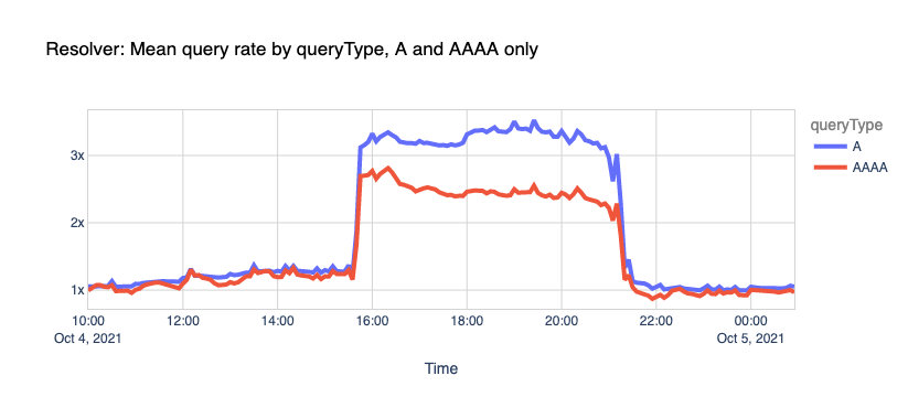
If we look at all the queries, not specific to Facebook or WhatsApp domains, and we split them by IPv4 and IPv6 clients, we can see that our load increased too.

As explained before, this is due to a snowball effect associated with applications and users retrying after the errors and generating even more traffic. In this case, 1.1.1.1 had to handle more than the expected rate for A and AAAA queries.

Here’s another fun one.

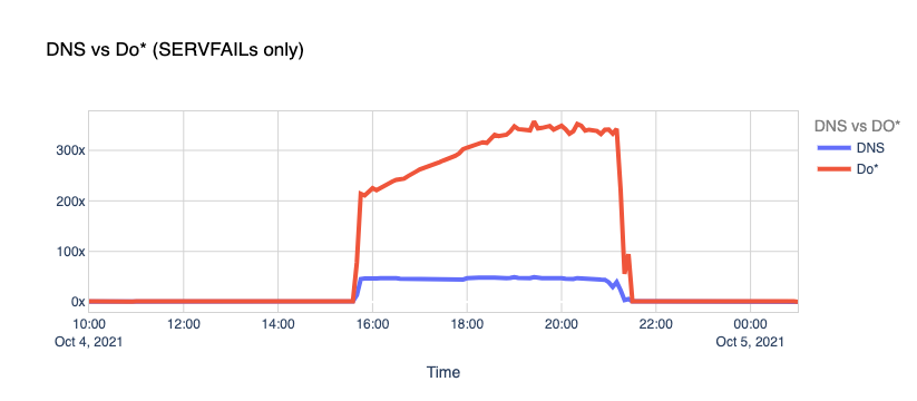
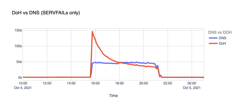
DNS vs. DoT and DoH. Typically, DNS queries and responses are sent in plaintext over UDP (or TCP sometimes), and that’s been the case for decades now. Naturally, this poses security and privacy risks to end-users as it allows in-transit attacks or traffic snooping.

With DNS over TLS (DoT) and DNS over HTTPS, clients can talk DNS using well-known, well-supported encryption and authentication protocols.

Our learning center has a good article on “DNS over TLS vs. DNS over HTTPS” that you can read. Browsers like Chrome, Firefox, and Edge have supported DoH for some time now, WAP uses DoH too, and you can even configure your operating system to use the new protocols.

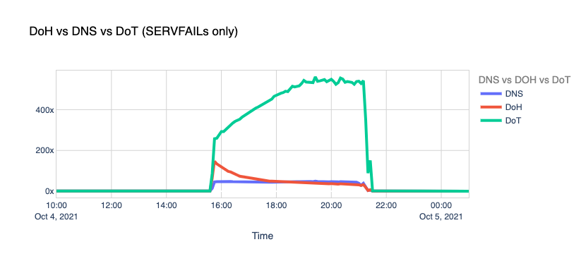
When Facebook went offline, we saw the number of DoT+DoH SERVFAILs responses grow by over x300 vs. the average rate.

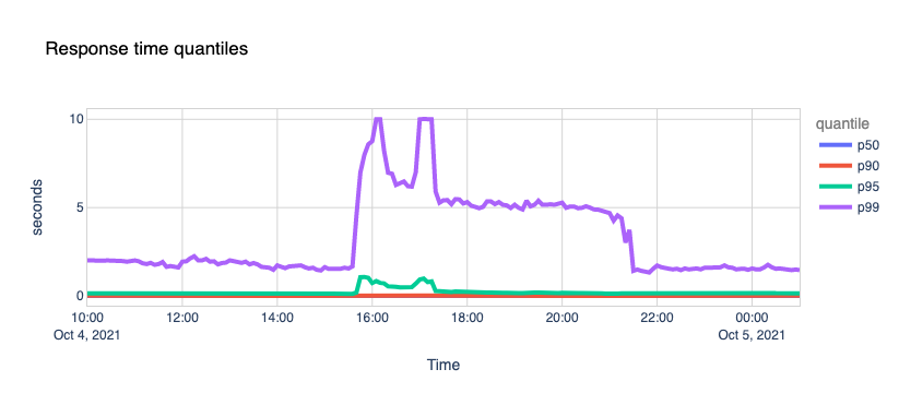
So, we got hammered with lots of requests and errors, causing traffic spikes to our 1.1.1.1 resolver and causing an unexpected load in the edge network and systems. How did we perform during this stressful period?

Quite well. 1.1.1.1 kept its cool and continued serving the vast majority of requests around the famous 10ms mark. An insignificant fraction of p95 and p99 percentiles saw increased response times, probably due to timeouts trying to reach Facebook’s nameservers.

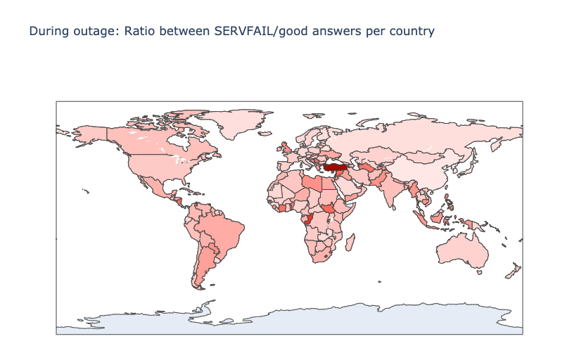
Another interesting perspective is the distribution of the ratio between SERVFAIL and good DNS answers, by country. In theory, the higher this ratio is, the more the country uses Facebook. Here’s the map with the countries that suffered the most:

Here’s the top twelve country list, ordered by those that apparently use Facebook, WhatsApp and Instagram the most:

Country	SERVFAIL/Good Answers ratio
Turkey	7.34
Grenada	4.84
Congo	4.44
Lesotho	3.94
Nicaragua	3.57
South Sudan	3.47
Syrian Arab Republic	3.41
Serbia	3.25
Turkmenistan	3.23
United Arab Emirates	3.17
Togo	3.14
French Guiana	3.00

Impact on other sites

When Facebook, Instagram, and WhatsApp aren’t around, the world turns to other places to look for information on what’s going on, other forms of entertainment or other applications to communicate with their friends and family. Our data shows us those shifts. While Facebook was going down, other services and platforms were going up.

To get an idea of the changing traffic patterns we look at DNS queries as an indicator of increased traffic to specific sites or types of site.

Here are a few examples.

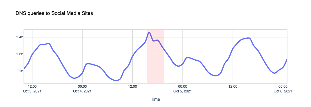
Other social media platforms saw a slight increase in use, compared to normal.

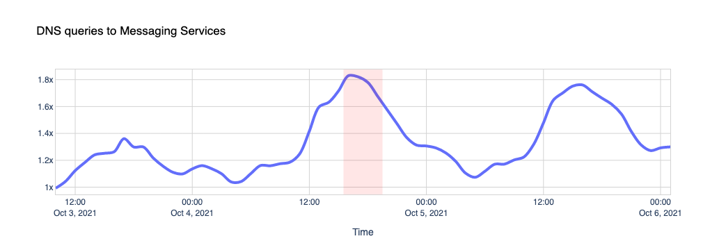
Traffic to messaging platforms like Telegram, Signal, Discord and Slack got a little push too.

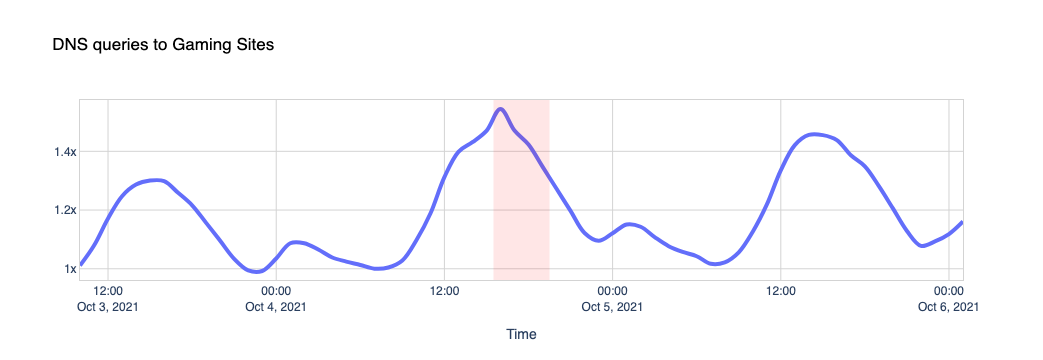
Nothing like a little gaming time when Instagram is down, we guess, when looking at traffic to sites like Steam, Xbox, Minecraft and others.

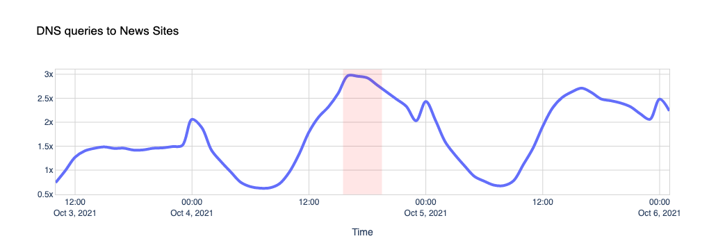
And yes, people want to know what’s going on and fall back on news sites like CNN, New York Times, The Guardian, Wall Street Journal, Washington Post, Huffington Post, BBC, and others:

Attacks

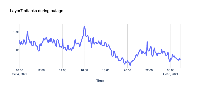
One could speculate that the Internet was under attack from malicious hackers. Our Firewall doesn’t agree; nothing out of the ordinary stands out.

Network Error Logs

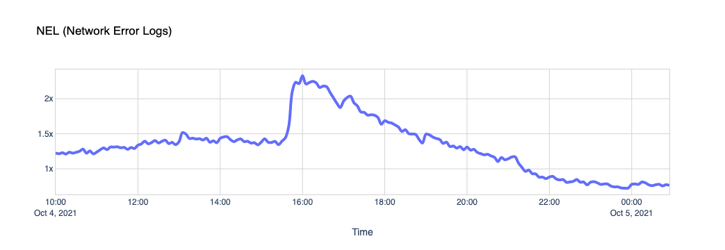
Network Error Logging, NEL for short, is an experimental technology supported in Chrome. A website can issue a Report-To header and ask the browser to send reports about network problems, like bad requests or DNS issues, to a specific endpoint.

Cloudflare uses NEL data to quickly help triage end-user connectivity issues when end-users reach our network. You can learn more about this feature in our help center.

If Facebook is down and their DNS isn’t responding, Chrome will start reporting NEL events every time one of the pages in our zones fails to load Facebook comments, posts, ads, or authentication buttons. This chart shows it clearly.

WARP

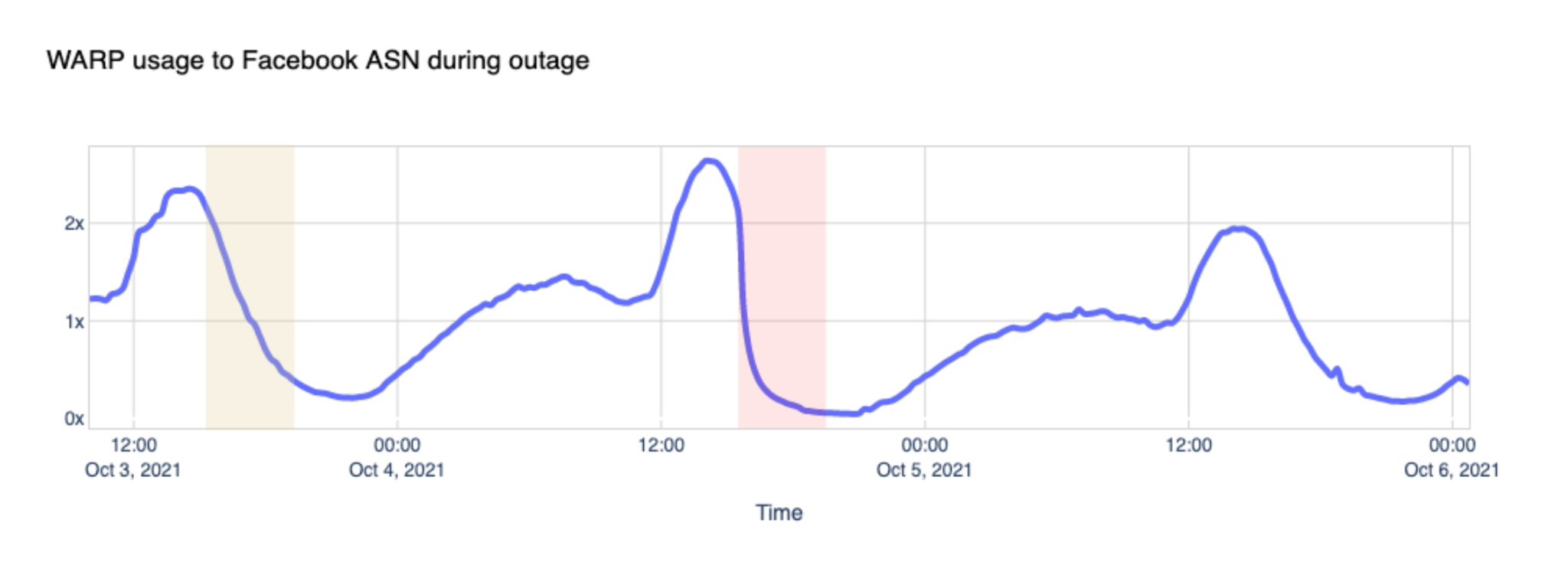
Cloudflare announced WARP in 2019, and called it “A VPN for People Who Don’t Know What V.P.N. Stands For” and offered it for free to its customers. Today WARP is used by millions of people worldwide to securely and privately access the Internet on their desktop and mobile devices. Here’s what we saw during the outage by looking at traffic volume between WARP and Facebook’s network:

You can see how the steep drop in Facebook ASN traffic coincides with the start of the incident and how it compares to the same period the day before.

Our own traffic

People tend to think of Facebook as a place to visit. We log in, and we access Facebook, we post. It turns out that Facebook likes to visit us too, quite a lot. Like Google and other platforms, Facebook uses an army of crawlers to constantly check websites for data and updates. Those robots gather information about websites content, such as its titles, descriptions, thumbnail images, and metadata. You can learn more about this on the “The Facebook Crawler” page and the Open Graph website.

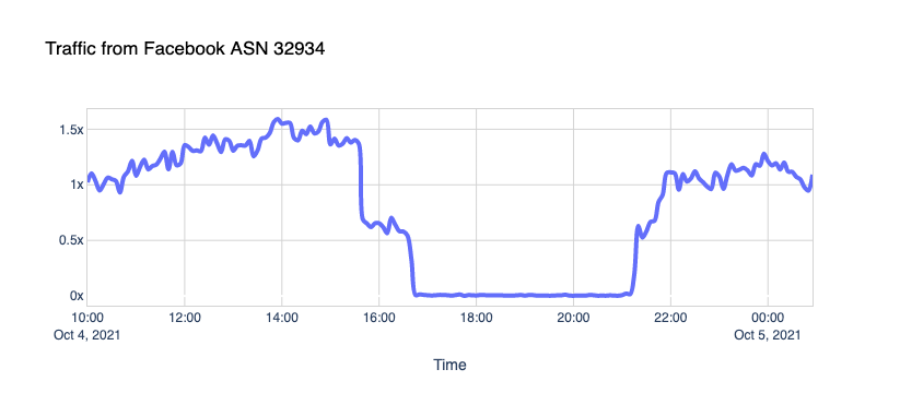
Here’s what we see when traffic is coming from the Facebook ASN, supposedly from crawlers, to our CDN sites:

The robots went silent.

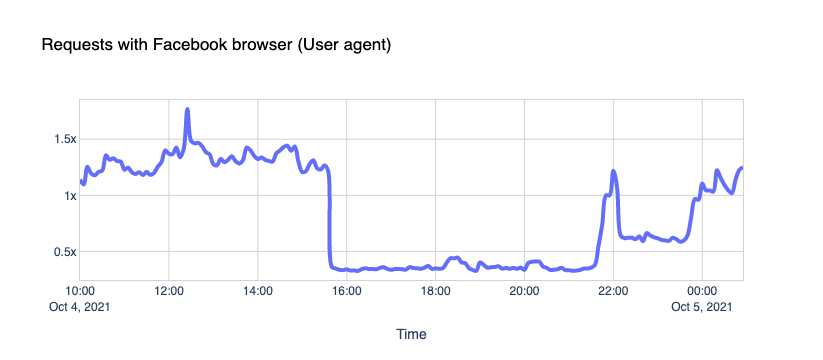
What about the traffic coming to our CDN sites from Facebook User-Agents? The gap is indisputable.

We see about 30% of a typical request rate hitting us. But it’s not zero; why is that?

We’ll let you know a little secret. Never trust User-Agent information; it’s broken. User-Agent spoofing is everywhere. Browsers, apps, and other clients deliberately change the User-Agent string when they fetch pages from the Internet to hide, obtain access to certain features, or bypass paywalls (because pay-walled sites want sites like Facebook to index their content, so that then they get more traffic from links).

Fortunately, there are newer, and privacy-centric standards emerging like User-Agent Client Hints.

Core Web Vitals

Core Web Vitals are the subset of Web Vitals, an initiative by Google to provide a unified interface to measure real-world quality signals when a user visits a web page. Such signals include Largest Contentful Paint (LCP), First Input Delay (FID), and Cumulative Layout Shift (CLS).

We use Core Web Vitals with our privacy-centric Web Analytics product and collect anonymized data on how end-users experience the websites that enable this feature.

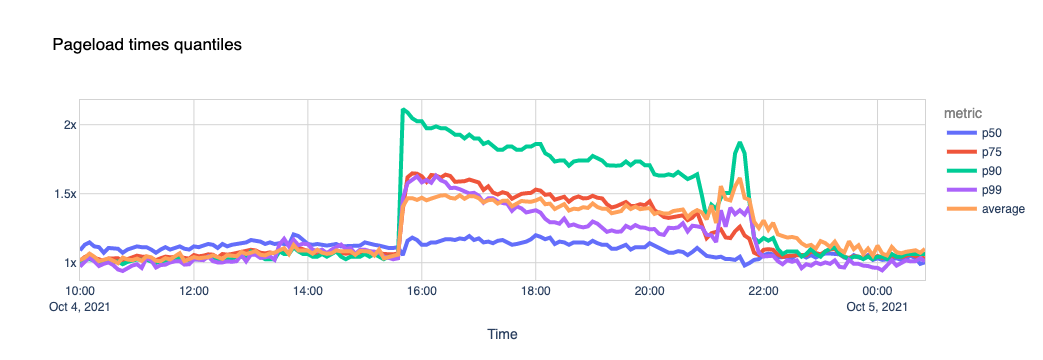
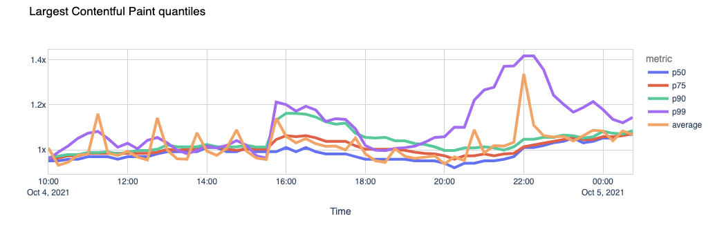
One of the metrics we can calculate using these signals is the page load time. Our theory is that if a page includes scripts coming from external sites (for example, Facebook “like” buttons, comments, ads), and they are unreachable, its total load time gets affected.

We used a list of about 400 domains that we know embed Facebook scripts in their pages and looked at the data.

Now let’s look at the Largest Contentful Paint. LCP marks the point in the page load timeline when the page’s main content has likely loaded. The faster the LCP is, the better the end-user experience.

Again, the page load experience got visibly degraded.

The outcome seems clear. The sites that use Facebook scripts in their pages took 1.5x more time to load their pages during the outage, with some of them taking more than 2x the usual time. Facebook’s outage dragged the performance of some other sites down.

Conclusion

When Facebook, Instagram, and WhatsApp went down, the Web felt it. Some websites got slower or lost traffic, other services and platforms got unexpected load, and people lost the ability to communicate or do business normally.

[$] Pulling slabs out of struct page

2021-10-08

Post Syndicated from original https://lwn.net/Articles/871982/rss

For the time being, the effort to add the folio
concept to the memory-management subsystem appears to be stalled, but appearances can
be deceiving. The numerous folio discussions have produced a number of
points of consensus, though; one of those is that far too much of the
kernel has to work with page structures to get its job done. As
an example of how a subsystem might be weaned off of struct page
usage, Matthew Wilcox has split out
the slab allocators in a 62-part patch set. The result may be
a foreshadowing of changes to come in the memory-management subsystem.

Weather Monitoring on a 486 PC! 1990s Davis Weather Station

2021-10-08 LGR

Post Syndicated from LGR original https://www.youtube.com/watch?v=QP2eP9MlGxU

Security updates for Friday

2021-10-08

Post Syndicated from original https://lwn.net/Articles/872267/rss

Security updates have been issued by Fedora (libssh), Mageia (firefox), Slackware (httpd), SUSE (xen), and Ubuntu (firefox and mysql-5.7).

What’s New in InsightVM: Q3 2021 in Review

2021-10-08 Sophie Johnson

Post Syndicated from Sophie Johnson original https://blog.rapid7.com/2021/10/08/whats-new-in-insightvm-q3-2021-in-review/

What's New in InsightVM: Q3 2021 in Review

In today’s post, we’re giving a rundown of new features and functionality launched in Q3 2021 for InsightVM and the Insight Platform. We hope you can begin to leverage these changes to drive success across your organization.

Apple Silicon support on the Insight Agent

We’re excited to announce that the Insight Agent now natively supports Apple Silicon chips!

Apple announced the first generation Apple Silicon chip — the M1 processor — in November 2020. This chip is the new standard on all MacBooks starting with the 2020 releases, and Apple plans to transition completely to Apple Silicon chips over the next two years.

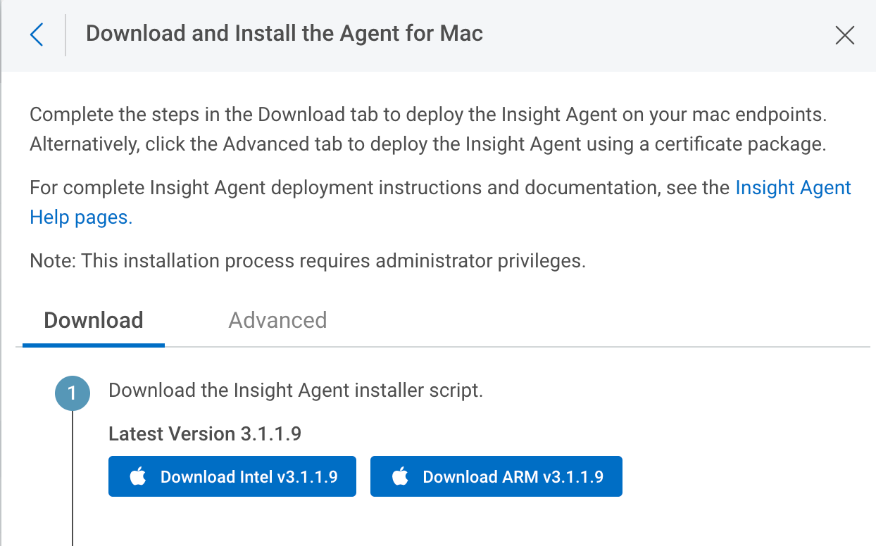
The new Mac installer specifically designed for the Apple Silicon can be accessed right from Agent Management in the platform, in the download section. Learn more in our Apple Silicon Agent Support blog post.

What's New in InsightVM: Q3 2021 in Review

Asset and Vulnerability Details reports

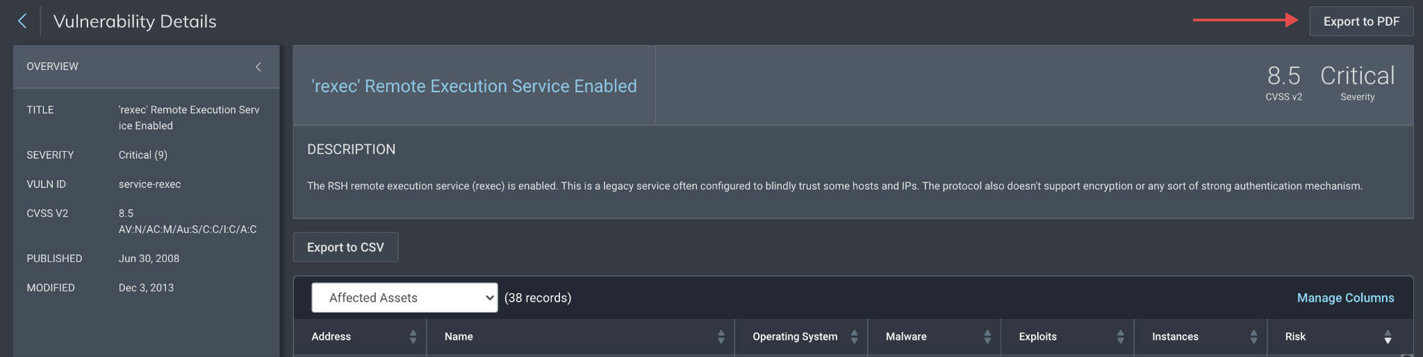
This new feature allows you to easily communicate details of your assets and vulnerabilities with stakeholders in a PDF format. Simply click the Export to PDF button on the Vulnerability Details page, and you’ll have a PDF ready to share!

This is particularly useful if you’re attempting to collaborate while remediating a specific vulnerability. We’ll use a hypothetical security engineer named Jane to illustrate this.

Jane recently read about a new ransomware strain that leverages a specific vulnerability as part of an attack chain that seems to be targeting the industry of her organization. She opens the query builder in InsightVM, constructs a search query to identify the vulnerability by CVE, and discovers several instances. She wants to mention this during her morning all-hands sync so she can recruit other team members to her effort. She exports the vulnerability details page to a PDF, which allows her to share this out and provide more details to interested team members, who then can help her remediate this vulnerability much more quickly.

Moreover, while undertaking this effort, another team member — Bill — finds an asset that seems to be a complete tragedy in terms of patching and vulnerability prevalence. He creates the Asset Details report and shares this in an e-mail to his team, stating that this asset seems to be missing their organization’s patch cycle. He also suggests that they look for more of these types of assets because he knows that when there is one offender, there are often many.

Snyk integration for reporting vulnerabilities

Container Security assessments will now report Ruby vulnerabilities through an integration with the Snyk vulnerability database. This adds RubyGems packages to our Snyk-based coverage, which currently includes vulnerability detections for Java, JavaScript, and Python libraries. This integration is particularly helpful for organizations that perform scanning of Container Images at rest, in both public and private registries.

Emergent threat coverage recap

Q3 2021 was another busy quarter for high-priority cybersecurity threats. As part of our emergent threat response process, Rapid7’s VRM research and engineering teams released vulnerability checks and in-depth technical analysis to help InsightVM customers understand the risk of exploitation and assess their exposure to critical security threats. In July, CVE-2021-34527, dubbed “PrintNightmare” presented remediation challenges for many organizations amid active exploitation of the Windows Print Spooler service. In August, the ProxyShell exploit chain put on-premises instances of Microsoft Exchange Server at risk for remote code execution. More recently, widespread attacks took advantage of CVE-2021-26084, a critical flaw in Confluence Server & Confluence Data Center, to deploy cryptominers, exfiltrate data, and obtain initial access for ransomware operations.

Other notable emergent threats included:

Stay tuned!

As always, we’re continuing to work on exciting product enhancements and releases throughout the year. Keep an eye on our blog and release notes as we continue to highlight the latest in vulnerability management at Rapid7.

NEVER MISS A BLOG

Get the latest stories, expertise, and news about security today.

Peshtigo: America’s Deadliest Fire

2021-10-08 The History Guy: History Deserves to Be Remembered

Post Syndicated from The History Guy: History Deserves to Be Remembered original https://www.youtube.com/watch?v=EidzEh6SMBs

ISOLATION – Photo Competition

2021-10-08 Matt Granger

Post Syndicated from Matt Granger original https://www.youtube.com/watch?v=zu8fMbmHRww

Helping Apache Servers stay safe from zero-day path traversal attacks (CVE-2021-41773)

2021-10-08 Michael Tremante

Post Syndicated from Michael Tremante original https://blog.cloudflare.com/helping-apache-servers-stay-safe-from-zero-day-path-traversal-attacks/

Helping Apache Servers stay safe from zero-day path traversal attacks (CVE-2021-41773)

On September 29, 2021, the Apache Security team was alerted to a path traversal vulnerability being actively exploited (zero-day) against Apache HTTP Server version 2.4.49. The vulnerability, in some instances, can allow an attacker to fully compromise the web server via remote code execution (RCE) or at the very least access sensitive files. CVE number 2021-41773 has been assigned to this issue. Both Linux and Windows based servers are vulnerable.

An initial patch was made available on October 4 with an update to 2.4.50, however, this was found to be insufficient resulting in an additional patch bumping the version number to 2.4.51 on October 7th (CVE-2021-42013).

Customers using Apache HTTP Server versions 2.4.49 and 2.4.50 should immediately update to version 2.4.51 to mitigate the vulnerability. Details on how to update can be found on the official Apache HTTP Server project site.

Any Cloudflare customer with the setting normalize URLs to origin turned on have always been protected against this vulnerability.

Additionally, customers who have access to the Cloudflare Web Application Firewall (WAF), receive additional protection by turning on the rule with the following IDs:

1c3d3022129c48e9bb52e953fe8ceb2f (for our new WAF)
100045A (for our legacy WAF)

The rule can also be identified by the following description:

Rule message: Anomaly:URL:Query String - Multiple Slashes, Relative Paths, CR, LF or NULL.

Given the nature of the vulnerability, attackers would normally try to access sensitive files (for example /etc/passwd), and as such, many other Cloudflare Managed Rule signatures are also effective at stopping exploit attempts depending on the file being accessed.

How the vulnerability works

The vulnerability leverages missing path normalization logic. If the Apache server is not configured with a require all denied directive for files outside the document root, attackers can craft special URLs to read any file on the file system accessible by the Apache process. Additionally, this flaw could also leak the source of interpreted files like CGI scripts and, in some cases, also allow the attacker to take over the web server by executing shell scripts.

For example, the following path:

$hostname/cgi-bin/../../../etc/passwd

would allow the attacker to climb the directory tree (../ indicates parent directory) outside of the web server document root and then subsequently access /etc/passwd.

Well implemented path normalization logic would correctly collapse the path into the shorter $hostname/etc/passwd by normalizing all ../ character sequences nullifying the attempt to climb up the directory tree.

Correct normalization is not easy as it also needs to take into consideration character encoding, such as percent encoded characters used in URLs. For example, the following path is equivalent to the first one provided:

$hostname/cgi-bin/.%2e/%2e%2e/%2e%2e/etc/passwd

as the characters %2e represent the percent encoded version of dot “.”. Not taking this properly into account was the cause of the vulnerability.

The PoC for this vulnerability is straightforward and simply relies on attempting to access sensitive files on vulnerable Apache web servers.

Exploit Attempts

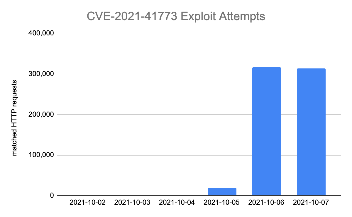
Cloudflare has seen a sharp increase in attempts to exploit and find vulnerable servers since October 5.

Most exploit attempts observed have been probing for static file paths — indicating heavy scanning activity before attackers (or researchers) may have attempted more sophisticated techniques that could lead to remote code execution. The most commonly attempted file paths are reported below:

/cgi-bin/.%2e/.git/config
/cgi-bin/.%2e/app/etc/local.xml
/cgi-bin/.%2e/app/etc/env.php
/cgi-bin/.%2e/%2e%2e/%2e%2e/etc/passwd

Conclusion

Keeping web environments safe is not an easy task. Attackers will normally gain access and try to exploit vulnerabilities even before PoCs become widely available — we reported such a case not too long ago with Atlassian’s Confluence OGNL vulnerability.

It is vital to employ all security measures available. Cloudflare features such as our URL normalization and the WAF, are easy to implement and can buy time to deploy any relevant patches offered by the affected software vendors.

Comic for 2021.10.08

2021-10-08 Explosm.net

Post Syndicated from Explosm.net original http://explosm.net/comics/5996/

New Cyanide and Happiness Comic

TSP vs TBSP

2021-10-08

Post Syndicated from original https://xkcd.com/2526/

It's like one teraspoon / when all you need is a kilonife

Align with best practices while creating infrastructure using CDK Aspects

2021-10-08 Om Prakash Jha

Post Syndicated from Om Prakash Jha original https://aws.amazon.com/blogs/devops/align-with-best-practices-while-creating-infrastructure-using-cdk-aspects/

Organizations implement compliance rules for cloud infrastructure to ensure that they run the applications according to their best practices. They utilize AWS Config to determine overall compliance against the configurations specified in their internal guidelines. This is determined after the creation of cloud resources in their AWS account. This post will demonstrate how to use AWS CDK Aspects to check and align with best practices before the creation of cloud resources in your AWS account.

The AWS Cloud Development Kit (CDK) is an open-source software development framework that lets you define your cloud application resources using familiar programming languages, such as TypeScript, Python, Java, and .NET. The expressive power of programming languages to define infrastructure accelerates the development process and improves the developer experience.

AWS Config is a service that enables you to assess, audit, and evaluate your AWS resource configurations. Config continuously monitors and records your AWS resource configurations, as well as lets you automate the evaluation of recorded configurations against desired configurations. React to non-compliant resources and change their state either automatically or manually.

AWS Config helps customers run their workloads on AWS in a compliant manner. Some customers want to detect it up front, and then only provision compliant resources. Some configurations are important for the customers, so they might not provision resources without having them compliant from the beginning. The following are examples of such configurations:

Amazon S3 bucket must not be created with public access
Amazon S3 bucket encryption must be enabled
Database deletion protection must be enabled

CDK Aspects

CDK Aspects are a way to apply an operation to every construct in a given scope. The aspect could verify something about the state of the constructs, such as ensuring that all buckets are encrypted, or it could modify the constructs, such as by adding tags.

An aspect is a class that implements the IAspect interface shown below. Aspects employ visitor patter, which allows them to add a new operation to existing object structures without modifying the structures. In object-oriented programming and software engineering, the visitor design pattern is a method for separating an algorithm from an object structure on which it operates.

interface IAspect {
   visit(node: IConstruct): void;
}

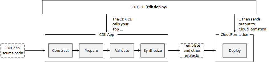
An AWS CDK app goes through the following lifecycle phases when you call cdk deploy. These phases are also shown in the diagram below. Learn more about the CDK application lifecycle at this page.

Construction
Preparation
Validation
Synthesis
Deployment

Understanding the CDK Deploy

CDK Aspects become relevant during the Prepare phase, where it makes the final modifications round in the constructs to setup their final state. This Prepare phase happens automatically. All constructs have their internal list of Aspects which are called and applied during the Prepare phase. Add your custom aspects in a scope by calling the following method:

Aspects.of(myConstruct).add(new SomeAspect(...));

When you call the method above, constructs add the custom aspects to the list of internal aspects. When CDK application goes through the Prepare phase, then AWS CDK calls the visit method of the object for the constructs and all of its children in top-down order. The visit method is free to change anything in the construct.

How to align with or check configuration compliance using CDK Aspects

In the following sections, you will see how to implement CDK Aspects for some common use cases when provisioning the cloud resources. CDK Aspects are extensible, and you can extend it for any suitable use cases in order to implement additional rules. Apply CDK Aspects not only to verify against the best practices, but also to update the state before resource creation.

The code below creates the cloud resources to be verified against the best practices or to be updated using Aspects in the following sections.

export class AwsCdkAspectsStack extends cdk.Stack {
  constructor(scope: cdk.Construct, id: string, props?: cdk.StackProps) {
    super(scope, id, props);

    //Create a VPC with 3 availability zones
    const vpc = new ec2.Vpc(this, 'MyVpc', {
      maxAzs: 3,
    });

    //Create a security group
    const sg = new ec2.SecurityGroup(this, 'mySG', {
      vpc: vpc,
      allowAllOutbound: true
    })

    //Add ingress rule for SSH from the public internet
    sg.addIngressRule(ec2.Peer.anyIpv4(), ec2.Port.tcp(22), 'SSH access from anywhere')

    //Launch an EC2 instance in private subnet
    const instance = new ec2.Instance(this, 'MyInstance', {
      vpc: vpc,
      machineImage: ec2.MachineImage.latestAmazonLinux(),
      instanceType: new ec2.InstanceType('t3.small'),
      vpcSubnets: {subnetType: ec2.SubnetType.PRIVATE},
      securityGroup: sg
    })

    //Launch MySQL rds database instance in private subnet
    const database = new rds.DatabaseInstance(this, 'MyDatabase', {
      engine: rds.DatabaseInstanceEngine.mysql({
        version: rds.MysqlEngineVersion.VER_5_7
      }),
      vpc: vpc,
      vpcSubnets: {subnetType: ec2.SubnetType.PRIVATE},
      deletionProtection: false
    })

    //Create an s3 bucket
    const bucket = new s3.Bucket(this, 'MyBucket')
  }
}

In the first section, you will see the use cases and code where Aspects are used to verify the resources against the best practices.

VPC CIDR range must start with specific CIDR IP
Security Group must not have public ingress rule
EC2 instance must use approved AMI

//Verify VPC CIDR range
export class VPCCIDRAspect implements IAspect {
    public visit(node: IConstruct): void {
        if (node instanceof ec2.CfnVPC) {
            if (!node.cidrBlock.startsWith('192.168.')) {
                Annotations.of(node).addError('VPC does not use standard CIDR range starting with "192.168."');
            }
        }
    }
}

//Verify public ingress rule of security group
export class SecurityGroupNoPublicIngressAspect implements IAspect {
    public visit(node: IConstruct) {
        if (node instanceof ec2.CfnSecurityGroup) {
            checkRules(Stack.of(node).resolve(node.securityGroupIngress));
        }

        function checkRules (rules :Array<IngressProperty>) {
            if(rules) {
                for (const rule of rules.values()) {
                    if (!Tokenization.isResolvable(rule) && (rule.cidrIp == '0.0.0.0/0' || rule.cidrIp == '::/0')) {
                        Annotations.of(node).addError('Security Group allows ingress from public internet.');
                    }
                }
            }
        }
    }
}

//Verify AMI of EC2 instance
export class EC2ApprovedAMIAspect implements IAspect {
    public visit(node: IConstruct) {
        if (node instanceof ec2.CfnInstance) {
            if (node.imageId != 'approved-image-id') {
                Annotations.of(node).addError('EC2 Instance is not using approved AMI.');
            }
        }
    }
}

In the second section, you will see the use cases and code where Aspects are used to update the resources in order to make them compliant before creation.

S3 bucket encryption must be enabled. If not, then enable
S3 bucket versioning must be enabled. If not, then enable
RDS instance must have deletion protection enabled. If not, then enable

//Enable versioning of bucket if not enabled
export class BucketVersioningAspect implements IAspect {
    public visit(node: IConstruct): void {
        if (node instanceof s3.CfnBucket) {
            if (!node.versioningConfiguration
                || (!Tokenization.isResolvable(node.versioningConfiguration)
                    && node.versioningConfiguration.status !== 'Enabled')) {
                Annotations.of(node).addInfo('Enabling bucket versioning configuration.');
                node.addPropertyOverride('VersioningConfiguration', {'Status': 'Enabled'})
            }
        }
    }
}

//Enable server side encryption for the bucket if no encryption is enabled
export class BucketEncryptionAspect implements IAspect {
    public visit(node: IConstruct): void {
        if (node instanceof s3.CfnBucket) {
            if (!node.bucketEncryption) {
                Annotations.of(node).addInfo('Enabling default S3 server side encryption.');
                node.addPropertyOverride('BucketEncryption', {
                        "ServerSideEncryptionConfiguration": [
                            {
                                "ServerSideEncryptionByDefault": {
                                    "SSEAlgorithm": "AES256"
                                }
                            }
                        ]
                    }
                )
            }
        }
    }
}

//Enable deletion protection of DB instance if not already enabled
export class RDSDeletionProtectionAspect implements IAspect {
    public visit(node: IConstruct) {
        if (node instanceof rds.CfnDBInstance) {
            if (! node.deletionProtection) {
                Annotations.of(node).addInfo('Enabling deletion protection of DB instance.');
                node.addPropertyOverride('DeletionProtection', true);
            }
        }
    }
}

Once you create the aspects, add them in a particular scope. That scope can be App, Stack, or Construct. In the example below, all aspects are added in the scope of Stack.

const app = new cdk.App();

const stack = new AwsCdkAspectsStack(app, 'MyApplicationStack');

Aspects.of(stack).add(new VPCCIDRAspect());
Aspects.of(stack).add(new SecurityGroupNoPublicIngressAspect());
Aspects.of(stack).add(new EC2ApprovedAMIAspect());
Aspects.of(stack).add(new RDSDeletionProtectionAspect());
Aspects.of(stack).add(new BucketEncryptionAspect());
Aspects.of(stack).add(new BucketVersioningAspect());

app.synth();

Once you call cdk deploy for the above code with aspects added, you will see the output below. The deployment will not continue until you resolve the errors and modifications conducted to make some of the resources compliant.

Screenshot displaying CDK errors.

Also utilize Aspects to make general modifications to the resources regardless of any compliance checks. For example, use it apply mandatory tags to every taggable resource. Tags is an example of implementing CDK Aspects in order to achieve this functionality. Utilizing the code below, add or remove a tag from all taggable resources and their children in the scope of a Construct.

Tags.of(myConstruct).add('key', 'value');
Tags.of(myConstruct).remove('key');

Below is an example of adding the Department tag to every resource created in the scope of Stack.

Tags.of(stack).add('Department', 'Finance');

CDK Aspects are ways for developers to align with and check best practices in their infrastructure configurations using the programming language of choice. AWS CloudFormation Guard (cfn-guard) provides compliance administrators with a simple, policy-as-code language to author policies and apply them to enforce best practices. Aspects are applied before generation of the CloudFormation template in Prepare phase, but cfn-guard is applied after generation of the CloudFormation template and before the Deploy phase. Developers can use Aspects or cfn-guard or both as part of a CI/CD pipeline to stop deployment of non-compliant resources, but CloudFormation Guard is the way to go when you want to enforce compliances and prevent deployment of non-compliant resources.

Conclusion

If you are utilizing AWS CDK to provision your infrastructure, then you can start using Aspects to align with best practices before resources are created. If you are utilizing CloudFormation template to manage your infrastructure, then you can read this blog to learn how to migrate the CloudFormation template to AWS CDK. After the migration, utilize CDK Aspects not only to evaluate compliance of your resources against the best practices, but also modify their state to make them compliant before they are created.

About the Authors

Target cross-platform Go builds with AWS CodeBuild Batch builds

2021-10-07 Russell Sayers

Post Syndicated from Russell Sayers original https://aws.amazon.com/blogs/devops/target-cross-platform-go-builds-with-aws-codebuild-batch-builds/

Many different operating systems and architectures could end up as the destination for our applications. By using a AWS CodeBuild batch build, we can run builds for a Go application targeted at multiple platforms concurrently.

Cross-compiling Go binaries for different platforms is as simple as setting two environment variables $GOOS and $GOARCH, regardless of the build’s host platform. For this post we will build all of the binaries on Linux/x86 containers. You can run the command go tool dist list to see the Go list of supported platforms. We will build binaries for six platforms: Windows+ARM, Windows+AMD64, Linux+ARM64, Linux+AMD64, MacOS+ARM64, and Mac+AMD64. Note that AMD64 is a 64-bit architecture based on the Intel x86 instruction set utilized on both AMD and Intel hardware.

This post demonstrates how to create a single AWS CodeBuild project by using a batch build and a single build spec to create concurrent builds for the six targeted platforms. Learn more about batch builds in AWS CodeBuild in the documentation: Batch builds in AWS CodeBuild

Solution Overview

AWS CodeBuild is a fully managed continuous integration service that compiles source code, runs tests, and produces ready-to-deploy software packages. A batch build is utilized to run concurrent and coordinated builds. Let’s summarize the 3 different batch builds:

Build graph: defines dependencies between builds. CodeBuild utilizes the dependencies graph to run builds in an order that satisfies the dependencies.
Build list: utilizes a list of settings for concurrently run builds.
Build matrix: utilizes a matrix of settings to create a build for every combination.

The requirements for this project are simple – run multiple builds with a platform pair of $GOOS and $GOARCH environment variables. For this, a build list can be utilized. The buildspec for the project contains a batch/build-list setting containing every environment variable for the six builds.

batch:
  build-list:
    - identifier: build1
      env:
        variables:
          GOOS: darwin
          GOARCH: amd64
    - identifier: build2
      env:
        variables:
          GOOS: darwin
          GOARCH: arm64
    - ...

The batch build project will launch seven builds. See the build sequence in the diagram below.

Step 1 – A build downloads the source.
Step 2 – Six concurrent builds configured with six sets of environment variables from the batch/build-list setting.
Step 3 – Concurrent builds package a zip file and deliver to the artifacts Amazon Simple Storage Service (Amazon S3) bucket.

build sequence

The supplied buildspec file includes commands for the install and build phases. The install phase utilizes the phases/install/runtime-versions phase to set the version of Go is used in the build container.

The build phase contains commands to replace source code placeholders with environment variables set by CodeBuild. The entire list of environment variables is documented at Environment variables in build environments. This is followed by a simple go build to build the binaries. The application getting built is an AWS SDK for Go sample that will list the contents of an S3 bucket.

  build:
    commands:
      - mv listObjects.go listObjects.go.tmp
      - cat listObjects.go.tmp | envsubst | tee listObjects.go
      - go build listObjects.go

The artifacts sequence specifies the build outputs that we want packaged and delivered to the artifacts S3 bucket. The name setting creates a name for ZIP artifact. And the name combines the operating system, architecture environment variables, as well as the git commit hash. We use Shell command language to expand the environment variables, as well as command substitution to take the first seven characters of the git hash.

artifacts:
  files:
    - 'listObjects'
    - 'listObjects.exe'
    - 'README.md'
  name: listObjects_${GOOS}_${GOARCH}_$(echo $CODEBUILD_RESOLVED_SOURCE_VERSION | cut -c 1-7).zip

Let’s walk through the CodeBuild project setup process. When the builds complete, we’ll see zip files containing the builds for each platform in an artifacts bucket.

Here is what we will create:

Create an S3 bucket to host the built artifacts.
Create the CodeBuild project, which needs to know:
- Where the source is
- The environment – a docker image and a service role
- The location of the build spec
- Batch configuration, a service role used to launch batch build groups
- The artifact S3 bucket location

The code that is built is available on github here: https://github.com/aws-samples/cross-platform-go-builds-with-aws-codebuild. For an alternative to the manual walkthrough steps, a CloudFormation template that will build all of the resources is available in the git repository.

Prerequisites

For this walkthrough, you must have the following prerequisites:

An AWS account
Access to an AWS account with administrator or PowerUser (or equivalent) AWS Identity and Access Management (IAM) role policies attached

Create the Artifacts S3 Bucket

An S3 bucket will be the destination of the build artifacts.

In the Amazon S3 console, create a bucket with a unique name. This will be the destination of your build artifacts.

Create the AWS CodeBuild Project

In the AWS CodeBuild console, create a project named multi-arch-build.
For Source Provider, choose GitHub. Choose the Connect to GitHub button and follow the authorization screens. For repository, enter https://github.com/aws-samples/cross-platform-go-builds-with-aws-codebuild
For Environment image, choose Managed Image. Choose the most recent Ubuntu image. This image contains every tool needed for the build. If you are interested in the contents of the image, then you can see the Dockerfile used to build the image in the GitHub repository here: https://github.com/aws/aws-codebuild-docker-images/tree/master/ubuntu
For Service Role, keep the suggested role name.
For Build specifications, leave Buildspec name empty. This will use the default location buildspec.yml in the source root.
Under Batch configuration, enable Define batch configuration. For the Role Name, enter a name for the role: batch-multi-arch-build-service-role. There is an option here to combine artifacts. CodeBuild can combine the artifacts from batch builds into a single location. This isn’t needed for this build, as we want a zip to be created for each platform.
Under Artifacts, for Type, choose Amazon S3. For Bucket name, select the S3 bucket created earlier. This is where we want the build artifacts delivered. Choose the checkbox for Enable semantic versioning. This will tell CodeBuild to use the artifact name that was specified in the buildspec file.
For Artifacts Packaging, choose Zip for CodeBuild to create a compressed zip from the build artifacts.
Create the build project, and start a build. You will see the DOWNLOAD_SOURCE build complete, followed by the six concurrent builds for each combination of OS and architecture.

Run the Artifacts

The builds have completed, and each packaged artifact has been delivered to the S3 bucket. Remember the name of the ZIP archive that was built using the buildspec file setting. This incorporated a combination of the operating system, architecture, and git commit hash.

Run the artifacts

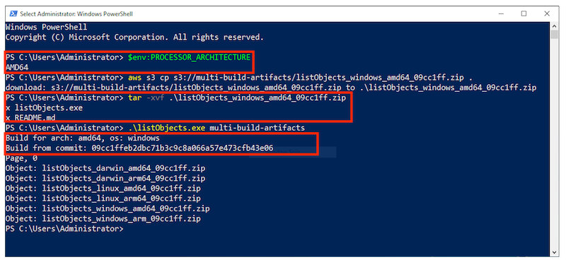
Below, I have tested the artifact by downloading the zip for the operating system and architecture combination on three different platforms: MacOS/AMD64, an AWS Graviton2 instance, and a Microsoft Windows instance. Note the system information, unzipping the platform artifact, and the build specific information substituted into the Go source code.

Cleaning up

To avoid incurring future charges, delete the resources:

On the Amazon S3 console, choose the artifacts bucket created, and choose Empty. Confirm the deletion by typing ‘permanently delete’. Choose Empty.
Choose the artifacts bucket created, and Delete.
On the IAM console, choose Roles.
Search for batch-multi-arch-build-service-role and Delete. Search for codebuild-multi-arch-build-service-role and Delete.
Go to the CodeBuild console. From Build projects, choose multi-arch-build, and choose Delete build project.

Conclusion

This post utilized CodeBuild batch builds to build and package binaries for multiple platforms concurrently. The build phase used a small amount of scripting to replace placeholders in the code with build information CodeBuild makes available in environment variables. By overriding the artifact name using the buildspec setting, we created zip files built from information about the build. The zip artifacts were downloaded and tested on three platforms: Intel MacOS, a Graviton ARM based EC2 instance, and Microsoft Windows.

Features like this let you build on CodeBuild, a fully managed build service – and not have to worry about maintaining your own build servers.

Prepare, transform, and orchestrate your data using AWS Glue DataBrew, AWS Glue ETL, and AWS Step Functions

2021-10-07 Durga Mishra

Post Syndicated from Durga Mishra original https://aws.amazon.com/blogs/big-data/prepare-transform-and-orchestrate-your-data-using-aws-glue-databrew-aws-glue-etl-and-aws-step-functions/

Data volumes in organizations are increasing at an unprecedented rate, exploding from terabytes to petabytes and in some cases exabytes. As data volume increases, it attracts more and more users and applications to use the data in many different ways—sometime referred to as data gravity. As data gravity increases, we need to find tools and services that allow us to prepare and process a large amount of data with ease to make it ready for consumption by a variety of applications and users. In this post, we look at how to use AWS Glue DataBrew and AWS Glue extract, transform, and load (ETL) along with AWS Step Functions to simplify the orchestration of a data preparation and transformation workflow.

DataBrew is a visual data preparation tool that exposes data in spreadsheet-like views to make it easy for data analysts and data scientists to enrich, clean, and normalize data to prepare it for analytics and machine learning (ML) without writing any line of code. With more than 250 pre-built transformations, it helps reduce the time it takes to prepare the data by about 80% compared to traditional data preparation approaches.

AWS Glue is a fully managed ETL service that makes it simple and cost-effective to categorize your data, clean it, enrich it, and move it reliably between various data stores and data streams. AWS Glue consists of a central metadata repository known as the AWS Glue Data Catalog, an ETL engine that automatically generates Python or Scala code, and a flexible scheduler that handles dependency resolution, job monitoring, and retries. AWS Glue is serverless, so there’s no infrastructure to set up or manage.

Step Functions is a serverless orchestration service that makes it is easy to build an application workflow by combining many different AWS services like AWS Glue, DataBrew, AWS Lambda, Amazon EMR, and more. Through the Step Functions graphical console, you see your application’s workflow as a series of event-driven steps. Step Functions is based on state machines and tasks. A state machine is a workflow, and a task is a state in a workflow that represents a single unit of work that another AWS service performs. Each step in a workflow is a state.

Overview of solution

DataBrew is a new service we introduced in AWS Re:invent 2020 in the self-serviced data preparation space and is focused on the data analyst, data scientist, and self-service audience. We understand that some organizations may have use cases where self-service data preparation needs to be integrated with a standard corporate data pipeline for advanced data transformation and operational reasons. This post provides a solution for customers who are looking for a mechanism to integrate data preparation done by analysts and scientists to the standard AWS Glue ETL pipeline using Step Functions. The following diagram illustrates this workflow.

Architecture overview

To demonstrate the solution, we prepare and transform the publicly available New Your Citi Bike trip data to analyze bike riding patterns. The dataset has the following attributes.

Field Name	Description
starttime	Start time of bike trip
stoptime	End time of bike trip
start_station_id	Station ID where bike trip started
start_station_name	Station name where bike trip started
start_station_latitude	Station latitude where bike trip started
start_station_longitude	Station longitude where bike trip started
end_station_id	Station ID where bike trip ended
end_station_name	Station name where bike trip ended
end_station_latitude	Station latitude where bike trip ended
end_station_longitude	Station longitude where bike trip ended
bikeid	ID of the bike used in bike trip
usertype	User type (customer = 24-hour pass or 3-day pass user; subscriber = annual member)
birth_year	Birth year of the user on bike trip
gender	Gender of the user (zero=unknown; 1=male; 2=female)

We use DataBrew to prepare and clean the most recent data and then use Step Functions for advanced transformation in AWS Glue ETL.

For the DataBrew steps, we clean up the dataset and remove invalid trips where either the start time or stop time is missing, or the rider’s gender isn’t specified.

After DataBrew prepares the data, we use AWS Glue ETL tasks to add a new column tripduration and populate it with values by subtracting starttime from endtime.

After we perform the ETL transforms and store the data in our Amazon Simple Storage Service (Amazon S3) target location, we use Amazon Athena to run interactive queries on the data to find the most used bikes to schedule maintenance, and the start stations with the most trips to make sure enough bikes are available at these stations.

We also create an interactive dashboard using Amazon QuickSight to gain insights and visualize the data to compare trip count by different rider age groups and user type.

The following diagram shows our solution architecture.

Prerequisites

To follow along with this walkthrough, you must have an AWS account. Your account should have permission to run an AWS CloudFormation script to create the services mentioned in solution architecture.

Your AWS account should also have an active subscription to QuickSight to create the visualization on processed data. If you don’t have a Quicksight account, you can sign up for an account.

Create the required infrastructure using AWS CloudFormation

To get started, complete the following steps:

Choose Launch Stack to launch the CloudFormation stack to configure the required resources in your AWS account.
On the Create stack page, choose Next.
On the Specify stack details page, enter values for Stack name and Parameters, and choose Next.
Follow the remaining instructions using all the defaults and complete the stack creation.

The CloudFormation stack takes approximately 2 minutes to complete.

When the stack is in the CREATE_COMPLETE state, go to the Resources tab of the stack and verify that you have 18 new resources.

In the following sections, we go into more detail of a few of these resources.

Source data and script files S3 bucket

The stack created an S3 bucket with the name formatted as <Stack name>-<SolutionS3BucketNameSuffix>.

On the Amazon S3 console, verify the creation of the bucket with the following folders:

scripts – Contains the Python script for the ETL job to process the cleaned data
source – Has the source City Bike data to be processed by DataBrew and the ETL job

DataBrew dataset, project, recipe, and job

The CloudFormation stack also created the DataBrew dataset, project, recipe, and job for the solution. Complete the following steps to verify that these resources are available:

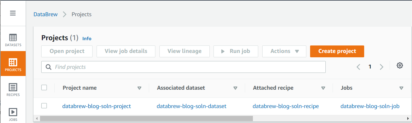
On the DataBrew console, choose Projects to see the list of projects.

You should see a new project, associated dataset, attached recipe, and job in the Projects list.

To review the source data, choose the dataset, and choose View dataset on the resulting popup.

You’re redirected to the Dataset preview page.

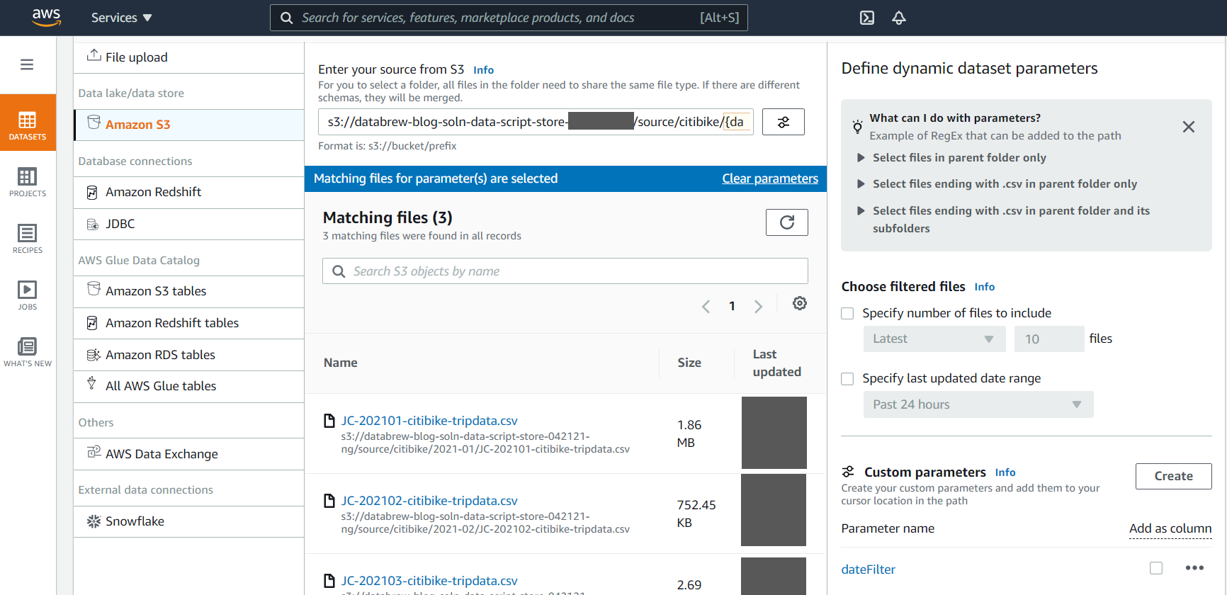
DataBrew lets you create a dynamic dataset using custom parameter and conditions. This feature helps you automatically process the latest files available in your S3 buckets with a user-friendly interface. For example, you can choose the latest 10 files or files that are created in the last 24 hours that match specific conditions to be automatically included in your dynamic dataset.

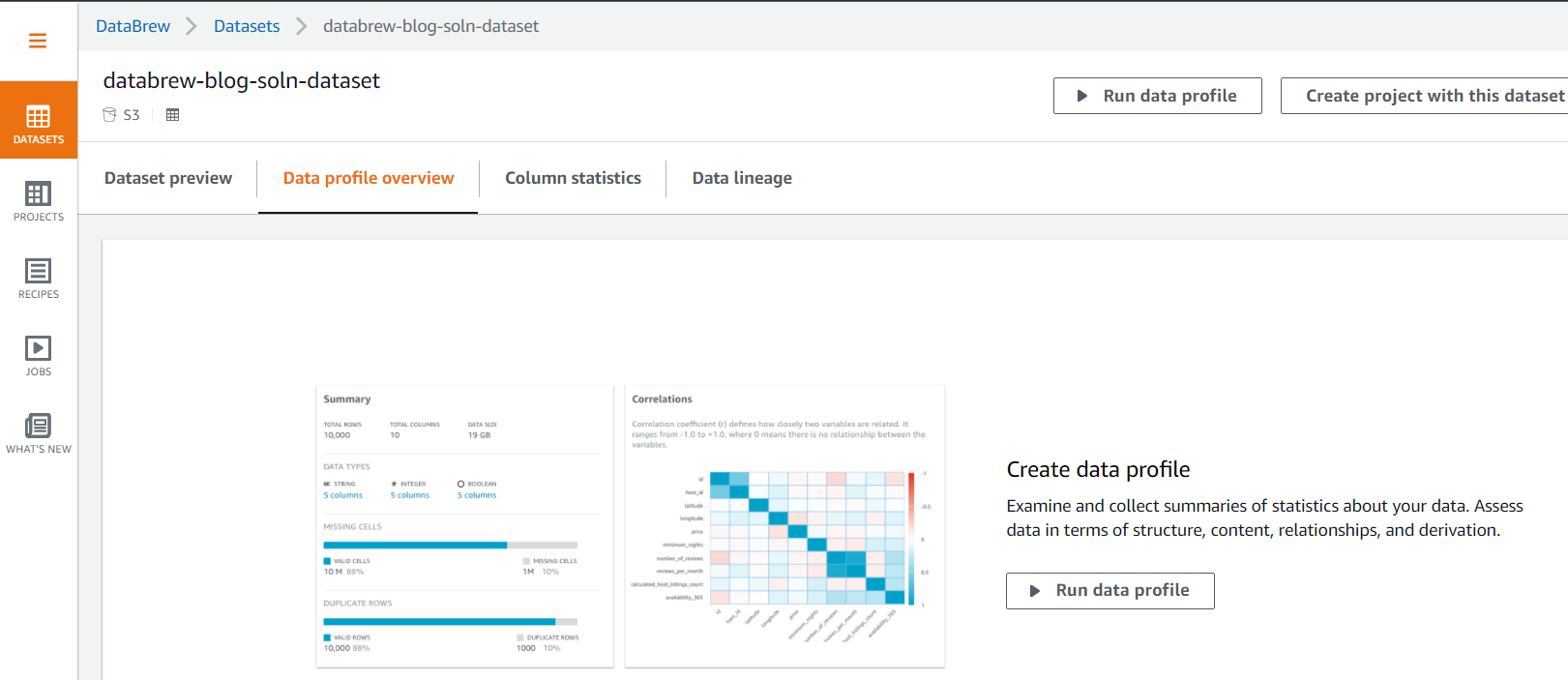
Choose the Data profile overview tab to examine and collect summaries of statistics about your data by running the data profile.
Choose Run data profile to create and run a profile job.
Follow the instructions to create and run the job to profile the source data.

The job takes 2–3 minutes to complete.

When the profiling job is complete, you should see Summary, Correlations, Value distribution, and Column Summary sections with more insight statistics about the data, including data quality, on the Data profile overview tab.

Choose the Column statistics tab to see more detailed statistics on individual data columns.

DataBrew provides a user-friendly way to prepare, profile, and visualize the lineage of the data. Appendix A at the end of this post provides details on some of the widely used data profiling and statistical features provided by DataBrew out of the box.

Choose the Data Lineage tab to see the information on data lineage.

Choose PROJECTS in the navigation pane and choose the project name to review the data in the project and the transformation applied through the recipe.

DataBrew provides over 250 transforms functions to prepare and transform the dataset. Appendix B at the end of this post reviews some of the most commonly used transformations.

We don’t need to run the DataBrew job manually—we trigger it using a Step Function state machine in subsequent steps.

AWS Glue ETL job

The CloudFormation stack also created an AWS Glue ETL job for the solution. Complete the following steps to review the ETL job:

On the AWS Glue console, choose Jobs in the navigation pane to see the new ETL job.
Select the job and on the Script tab, choose Edit script to inspect the Python script for the job.

We don’t need to run the ETL job manually—we trigger it using a Step Function state machine in subsequent steps.

Start the Step Function state machine

The CloudFormation stack created a Step Functions state machine to orchestrate running the DataBrew job and AWS Glue ETL job. A Lambda function starts the state machine whenever the daily data files are uploaded into the source data folder of the S3 bucket. For this post, we start the state machine manually.

On the Step Functions console, choose State machines in the navigation pane to see the list of state machines.
Choose the state machine to see the state machine details.
Choose Start execution to run the state machine.

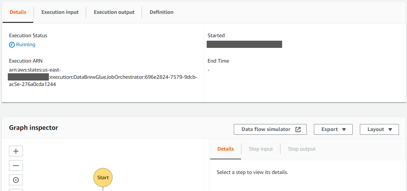
The details of the state machine run are displayed on the Details tab.

Review the Graph inspector section to observe the different states of the state machine. As each step completes, it turns green.

Choose the Definition tab to review the definition of the state machine.

When the state machine is complete, it should have run the DataBrew job to clean the data and the AWS Glue ETL job to process the cleaned data.

The DataBrew job removed all trips in the source dataset with missing starttime and stoptime, and unspecified gender. It also copied the cleaned data to the cleaned folder of the S3 bucket. We review the cleaned data in subsequent steps with Athena.

The ETL job processed the data in the cleaned folder to add a calculated column tripduration, which is calculated by subtracting the starttime from the stoptime. It also converted the processed data into columnar format (Parquet), which is more optimized for analytical processing, and copied it to the processed folder. We review the processed data in subsequent steps with Athena and also use it with QuickSight to get some insight into rider behavior.

Run an AWS Glue crawler to create tables in the Data Catalog

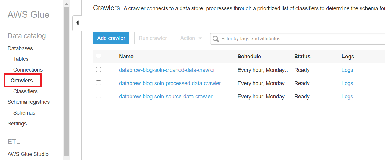
The CloudFormation stack also added three AWS Glue crawlers to crawl through the data stored in the source, cleaned, and processed folders. A crawler can crawl multiple data stores in a single run. Upon completion, the crawler creates or updates one or more tables in your Data Catalog. Complete the following steps to run these crawlers to create AWS Glue tables for the date in each of the S3 folders.

On the AWS Glue console, choose Crawlers in the navigation pane to see the list of crawlers created by the CloudFormation stack.If you have AWS Lake Formation enabled in the Region in which you’re implementing this solution, you may get insufficient lake formation permissions error. Please follow steps in Appendix C to provide required permission to the IAM role used by Glue Crawler to create table in citibike database.
Select each crawler one by one and choose Run crawler.

After the crawlers successfully run, you should see one table added by each crawler.

We run crawlers manually in this post, but you can trigger the crawlers whenever a new file is added to their respective S3 bucket folder.

To verify the AWS Glue database citibike, created by the CloudFormation script, choose Databases in the navigation pane.
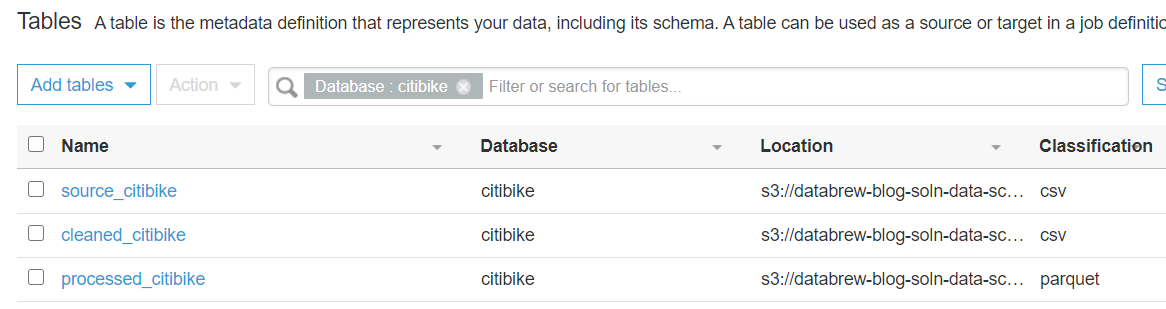
Select the citibike database and choose View tables.

You should now see the three tables created by the crawlers.

Use Athena to run analytics queries

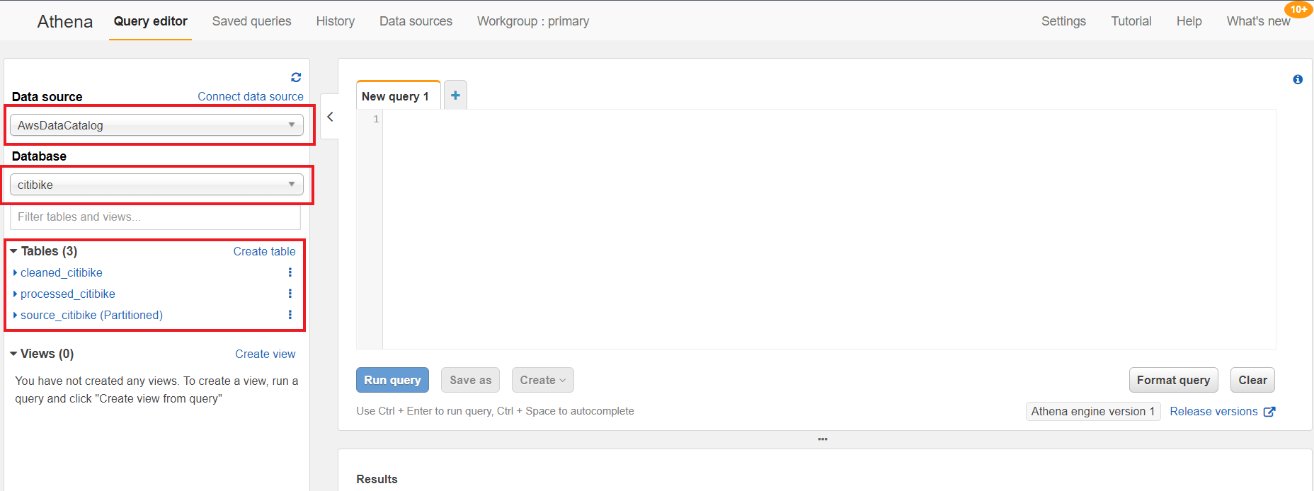
In the following steps, we use Athena for ad-hoc analytics queries on the cleaned and processed data in the processed_citibike table of the Data Catalog. For this post, we find the 20 most used bikes to schedule maintenance for them, and find the top 20 start stations with the most trips to make sure enough bikes are available at these stations.

On the Athena console, for Data source, choose AwsDataCatalog.
For Database, choose citibike.

The three new tables are listed under Tables.

If you haven’t used Athena before in your account, you receive a message to set up a query result location for Athena to store the results of queries.

Run the following query on the New query1 tab to find the find the 20 most used bikes:

SELECT bikeid as BikeID, count(*) TripCount FROM "citibike"."processed_citibike" group by bikeid order by 2 desc limit 20;

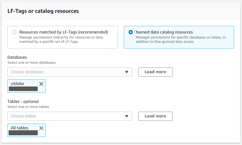
If you have AWS Lake Formation enabled in the Region in which you’re implementing this solution, you may get error (similar to below error) in executing queries. To resolve the permission issues, please follow steps in Appendix D to provide “Select” permission to all tables in citibike database to logged in user using Lake Formation.

Run the following query on the New query1 tab to find the top 20 start stations with the most trips:

SELECT start_station_name, count(*) trip_count FROM "citibike"."processed_citibike" group by start_station_name order by 2 desc limit 20;

Visualize the processed data on a QuickSight dashboard

As the final step, we visualize the following data using a QuickSight dashboard:

Compare trip count by different rider age groups
Compare trip count by user type (customer = 24-hour pass or 3-day pass user; subscriber = annual member)

Your AWS account should also have an active subscription to QuickSight to create the visualization on processed data. If you don’t have a Quicksight account, you can sign up for an account.

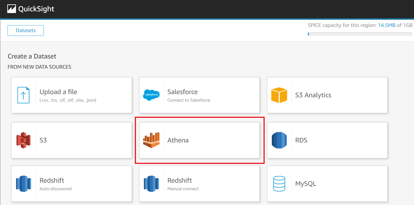
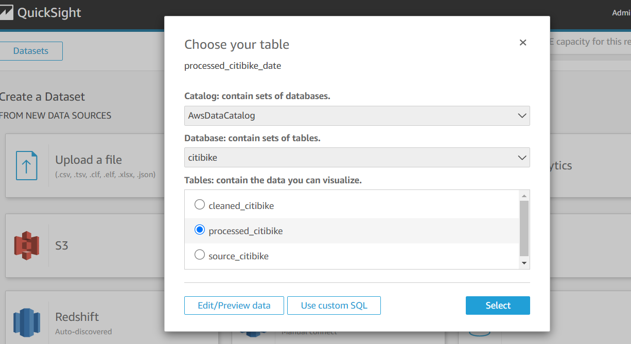
On the QuickSight console, create a dataset with Athena as your data source.
Follow the instructions to complete your dataset creation.
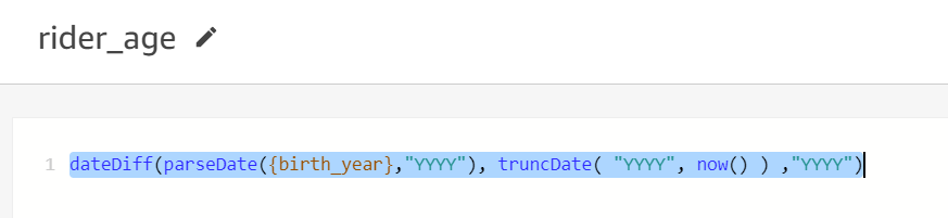
Add a calculated filed rider_age using following formula:

dateDiff(parseDate({birth_year},"YYYY"), truncDate( "YYYY", now() ) ,"YYYY")

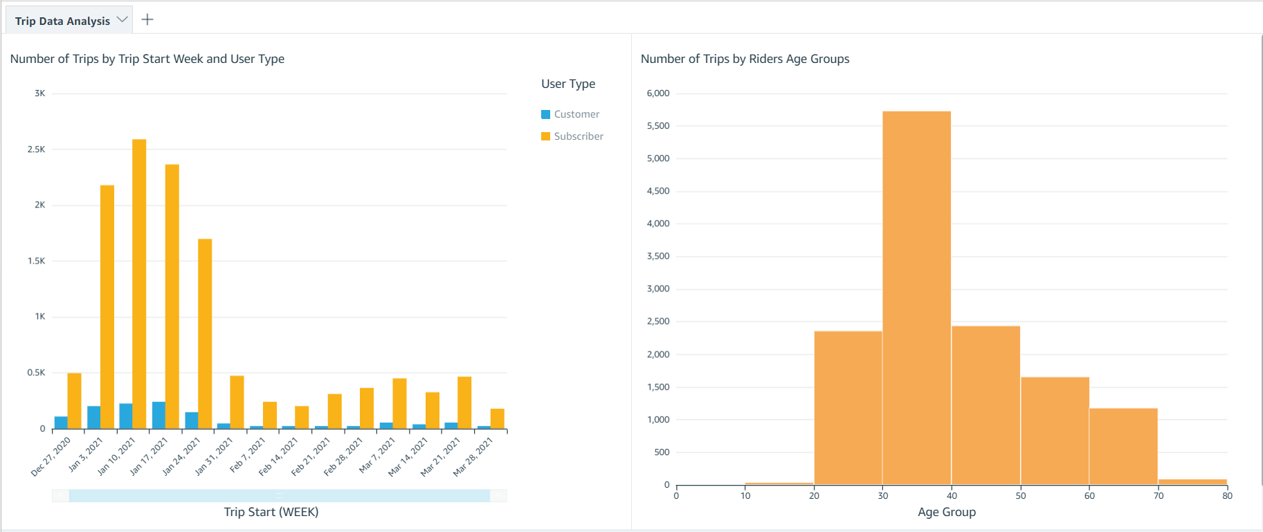
Your dataset should look like the following screenshot.

Now you can create visualizations to compare weekly trip count by user type and total trip count by rider age group.

Clean up

To avoid incurring future charges, delete the resources created for the solution.

Delete the DataBrew profile job created for profiling the source data.
Delete the CloudFormation stack to delete all the resources created by the stack.

Conclusion

In this post, we discussed how to use DataBrew to prepare your data and then further process the data using AWS Glue ETL to integrate it in a standard operational ETL flow to gather insights from your data.

We also walked through how you can use Athena to perform SQL analysis on the dataset and visualize and create business intelligence reports through QuickSight.

We hope this post provides a good starting point for you to orchestrate your DataBrew job with your existing or new data processing ETL pipelines.

For more details on using DataBrew with Step Functions, see Manage AWS Glue DataBrew Jobs with Step Functions.

For more information on DataBrew jobs, see Creating, running, and scheduling AWS Glue DataBrew jobs.

Appendix A

The following table lists the widely used data profiling and statistical features provided by DataBrew out of the box.

Type	Data type of the column
`missingValuesCount`	The number of missing values. Null and empty strings are considered as missing.
`distinctValuesCount`	The number of the value appears at least once.
`entropy`	A measure of the randomness in the information being processed. The higher the `entropy`, the harder it is to draw any conclusions from that information.
`mostCommonValues`	A list of the top 50 most common values.
`mode`	The value that appears most often in the column.
`min/max/range`	The minimum, maximum, and range values in the column.
`mean`	The mean or average value of the column.
`kurtosis`	A measure of whether the data is heavy-tailed or light-tailed relative to a normal distribution. A dataset with high `kurtosis` has more outliers compared to a dataset with low `kurtosis`.
`skewness`	A measure of the asymmetry of the probability distribution of a real-valued random variable about its mean.
`Correlation`	The Pearson correlation coefficient. This is a measure if one column’s values correlate to values of another column.
`Percentile95`	The element in the list that represents the 95th percentile (95% of numbers fall below this and 5% of numbers fall above it).
`interquartileRange`	The range between the 25th percentile and 75th percentile of numbers.
`standardDeviation`	The unbiased sample standard deviation of values in the column.
`min/max Values`	A list of the five minimum and maximum values in a column.
`zScoreOutliersSample`	A list of the top 50 outliers that have the largest or smallest Z-score. -/+3 is the default threshold.
`valueDistribution`	The measure of the distribution of values by range.

Appendix B

DataBrew provides the ability to prepare and transform your dataset using over 250 transforms. In this section, we discuss some of the most commonly used transformations:

Combine datasets – You can combine datasets in the following ways:
- Join – Combine several datasets by joining them with other datasets using a join type like inner join, outer join, or excluding join.
- Union operation – Combine several datasets using a union operation.
- Multiple files for input datasets – While creating a dataset, you can use a parameterized Amazon S3 path or a dynamic parameter and select multiple files.
Aggregate data – You can aggregate the dataset using a group by clause and use standard and advanced aggregation functions like Sum, Count, Min, Max, mode, standard deviation, variance, skewness, kurtosis, as well as cumulative functions like cumulative sum and cumulative count.
Pivot a dataset – You can pivot the dataset in the following ways:
- Pivot operation – Convert all rows to columns.
- Unpivot operation – Convert all columns to rows.
- Transpose operation – Convert all selected rows to columns and columns to rows.
Unnest top level value – You can extract values from arrays into rows and columns into rows. This only operates on top-level values.
Outlier detection and handling – This transformation works with outliers in your data and performs advanced transformations on them like flag outliers, rescale outliers, and replace or remover outliers. You can use several strategies like ZScore, modified Z-score, and interquartile range (IQR) to detect outliers.
Delete duplicate values – You can delete any row that is an exact match to an earlier row in the dataset.
Handle or impute missing values – You have the following options:
- Remove invalid records – Delete an entire row if an invalid value is encountered in a column of that row.
- Replace missing values – Replace missing values with custom values, most frequent value, last valid value, or numeric aggregate values.
Filter data – You can filter the dataset based on a custom condition, validity of a column, or missing values.
Split or merge columns – You can split a column into multiple columns based on a custom delimiter, or merge multiple columns into a single column.
Create columns based on functions –You can create new columns using different functions like mathematical functions, aggregated functions, date functions, text functions, windows functions like next and previous, and rolling aggregation functions like rolling sum, rolling count, and rolling mean.

Appendix C

If you have AWS Lake Formation enabled in the Region in which you’re implementing this solution, you may get insufficient lake formation permissions error during Glue Crawler run.

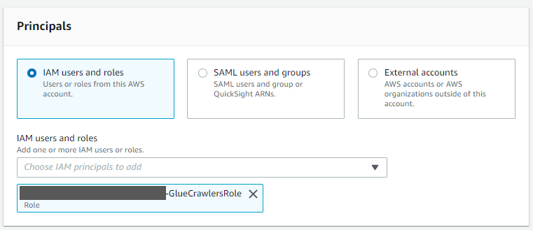
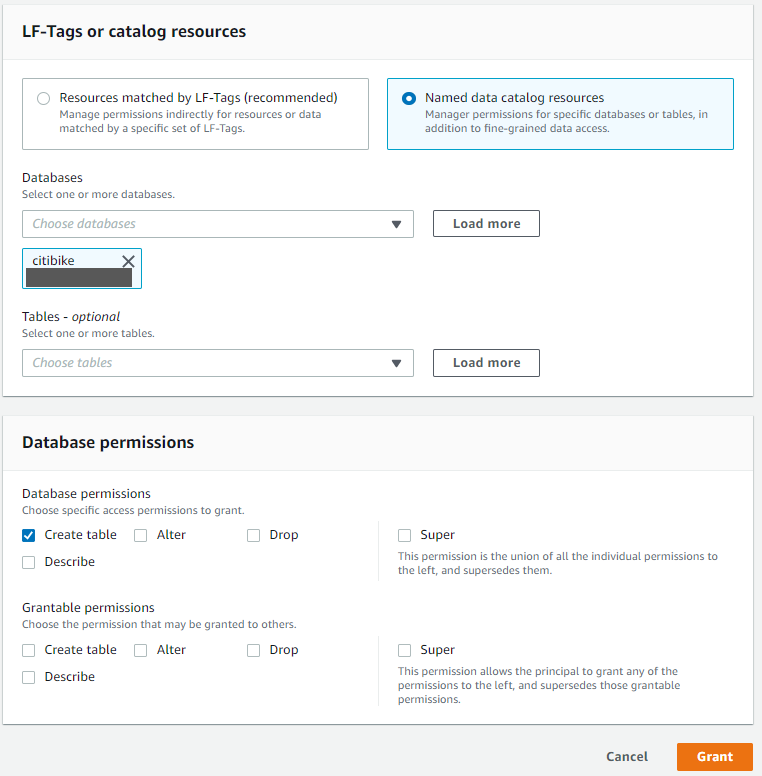
Please provide create table permission in GlueDatabase (citibike) to GlueCrawlersRole (find the ARN from the Cloud Formation Resource section) for the crawler to create required table.

Appendix D

If you have AWS Lake Formation enabled in the Region in which you’re implementing this solution, you may get error similar to below error in running queries on tables in citibike database.

Please provide “Select” permission to all tables in GlueDatabase (citibike) to logged in user in Lake formation to allow the select on tables created by the solution to logged in user.

About the Authors

Photo and bio go here Narendra Gupta is a solutions architect at AWS, helping customers on their cloud journey with focus on AWS analytics services. Outside of work, Narendra enjoys learning new technologies, watching movies, and visiting new places.

Photo and bio go hereDurga Mishra is a solutions architect at AWS. Outside of work, Durga enjoys spending time with family and loves to hike on Appalachian trails and spend time in nature.

Photo and bio go hereJay Palaniappan is a Sr. Analytics Specialist Solutions architect at AWS, helping media & entertainment customers adopt and run AWS Analytics services.

Stable kernels 5.14.10 and 4.4.287

2021-10-07

Post Syndicated from original https://lwn.net/Articles/872194/rss

Stable kernels 5.14.10 and 4.4.287 have been released. 5.14.10 is a
standard stable release, with fixes throughout the kernel tree, while
4.4.287 is fixing a build problem: “You only need this release if you
are building for ARM64 and had build failures
with 4.4.286.”

How to Be Self-Aware – How To Build a Happy Life, Ep. 1, with Dan Harris

2021-10-07 The Atlantic

Post Syndicated from The Atlantic original https://www.youtube.com/watch?v=2_16NNKZFuI

Safe Updates of Client Applications at Netflix

2021-10-07 Netflix Technology Blog

Post Syndicated from Netflix Technology Blog original https://netflixtechblog.com/safe-updates-of-client-applications-at-netflix-1d01c71a930c

By Minal Mishra

Quality of a client application is of paramount importance to global digital products, as it is the primary way customers interact with a brand. At Netflix, we have significant investments in ensuring new versions of our applications are well tested. However, Netflix is available for streaming on thousands of types of devices and it is powered by hundreds of micro-services which are deployed independently, making it extremely challenging to comprehensively test internally. Hence, it became important to supplement our release decisions with strong evidence received from the field during the update process.

Our team was formed to mine health signals from the field to quickly evaluate new versions of the client applications. As we invested in systems to enable this vision, it led to increased development velocity, which arguably led to better development practices and quality of the applications. The goal of this blog post is to highlight the investment areas for this vision and the challenges we are facing today.

Client Applications

We deal with two classes of client application updates. The first is where an application package is downloaded from the service or a CDN. An example of this is Netflix’s video player or the TV UI javascript package. The second is one where an application is hosted behind an app store, for example mobile phones or even game consoles. We have more flexibility to control the distribution of the application in the former than in the latter case.

Deployment Strategies

We are all familiar with the advantages of releasing frequently and in smaller chunks. It helps bring a healthy balance to the velocity and quality equation. The challenge for clients is that each instance of the application runs on a Netflix member’s device and signals are derived from a firehose of events being sent by devices across the globe. Depending on the type of client, we need to determine the right strategy to sample consumer devices, and provide a system that can enable various client engineering teams to look for their signals. Hence, the sampling strategy is different if it is a mobile application versus a smart TV. In contrast, a server application runs on servers which are typically identical and a routing abstraction can serve sampled traffic to new versions. And the signals to evaluate a new version are derived from comparatively few thousands of homogenous servers instead of millions of heterogeneous devices.

**Staged rollouts** of apps mimic the different phases of moon

A widely adopted technique for client applications is gradually rolling out a new version of software rather than making the release available to all users instantly, also known as staged or phased rollout. There are two main benefits to this approach.

First, if something were to fail catastrophically, the release can be paused for triage, limiting the number of customers impacted.
Second, backend services or infrastructure can be scaled intelligently as adoption ramps up.

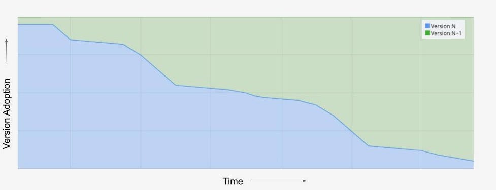
Application version adoption over time for a **staged rollout**

This chart represents a counter metric, which exhibits version adoption over the duration of a staged rollout. There is a gradual increase in the percentage of devices switching to N+1 version. In the past, during this period client engineering teams would visually monitor their metric dashboards to evaluate signals as more consumers migrated to a new version of their application.

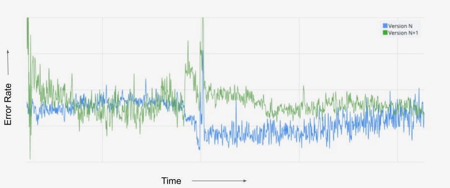
Client-side error rate during the **staged rollout**

The chart of client-side error rate during the same time period as the version migration is shown here. We observe that the metric for the new version N+1 stabilizes as the rollout ramps up and reaches closer to 100%, whereas the metric for the current version N becomes noisy over the same time duration. Trying to compare any metric during this time period can be a futile effort, as obvious in this case where there was no customer impacting shift in the error rate but we cannot interpret that from the chart. Typically, teams time-shift one metric over the other to visually detect metric deviations, but time can still be a confounder. Staged rollouts have a lot of benefits, but there is a significant opportunity cost to wait before the new version reaches a critical level of adoption.

AB Tests/Client Canaries

So we brought the science of controlled testing into this decision framework by using what has been utilized for feature evaluations. The main goal of A/B testing is to design a robust experiment that is going to yield repeatable results and enable us to make sound decisions about whether or not to launch a product feature (read more about A/B tests at Netflix here). In the application update use case, we recommend an extreme version of A/B testing: we test the entire application. The new version may include a user facing feature which is designed to be A/B tested and resides behind a feature flag. However, most times it is adding new obvious improvements, simple bug fixes, performance enhancements, productizing outcomes from previous A/B tests, logging etc that are being shipped in the application. If we apply A/B tests methodology (or client canaries as we like to call them to differentiate from traditional feature based A/B tests) the allocation would look identical for both the versions at any time.

Client Canary and Control allocation along with the client-side error rate metric

This chart is showing the new and the baseline version allocations growing over time. Although, majority of users are already on the baseline version we are randomly “allocating” a fraction of those users to be the control group of our experiment. This ensures there is no sampling mismatch between the treatment and the control group. It is easier to visually compare the client side error rate for both versions and even apply statistical inference to change the conversation from “we think” there is a shift in metrics to “we know”.

But there are differences between feature related A/B tests at Netflix and the incremental product changes used for Client Canaries. The main distinctions are: a shorter runtime, multiple executions of analysis sometimes concurrent with allocation, and use of data to support the null hypothesis. The runtime is predetermined, which in a way, is the stopping rule for client canaries. Unlike feature A/B tests at Netflix, we limit our evidence collection to a few hours, so we can release updates within a working day. We continuously analyze metrics to find egregious regressions sooner rather than once all the evidence has been collected.

The three key phases of any A/B tests can be split into Allocation, Metric Collection and Analysis. We use orchestration to connect and manage client applications through the A/B test lifecycle, thereby reducing the cognitive load of deploying them frequently.

Allocation

Sampling is the first stage once your new application has been packaged, tested and published. As time is of the essence here, we rely on dynamic allocation and allocate devices which come to the service during the canary time period based on pre-configured rules. We leverage the allocation service used for all experimentation at Netflix for this purpose.

However, for applications gated behind an external app store (example mobile apps), we only have access to staged rollout solutions provided by the app stores. We can control the percentage of users receiving updated apps, which can increase over time. In order to mimic the client canary solution, we built a synthetic allocation service to perform sampling post-installation of the app updates. This service tries to allocate a device to the control group that typically matches the profile of a device seen in the treatment group, which was allocated by the app store’s staged rollout solution. This ensures we are controlling for key variables which have the potential to impact the analysis.

Metrics

Metrics are a foundational component for client canaries and A/B tests as they give us the necessary insight required to make decisions. And for our use case, metrics need to be computed in real time from millions of user events being sent to our service. Operating at Netflix’s scale, we have to process the event streams on a scalable platform like Mantis and store the time-series data in Apache Druid. To be further cost-efficient with the time-series data we store the metrics for a sliding time window of a few weeks and compress it to a 1 minute time granularity.

The other challenge is to enable client application engineers to contribute to metrics and dimensions as they are aware of what can be a valuable insight. To do this, our real-time metric data pipeline provides the right abstractions to remove the complexity of a distributed stream processing system and also enables these contributions to be used in offline computations for feature A/B test evaluations.The former reduces the barrier to entry and the latter provides additional motivation for client engineers to contribute. Additionally, this gets us closer to consistent metric definitions in both realtime and offline systems.

As we accept contributions, we have to have the right checks in place to ensure the data pipeline is reliable and robust. Changes in user events, stream processing jobs or even in the platform can impact metrics, and so it is imperative that we actively monitor the data pipeline and ingestion.

Analysis

Historically, we have relied on conventional statistical tests built into Kayenta to detect metric shifts for the release of new versions of applications. It has served us well over the last few years, however at Netflix we are always looking to improve. Some reasons to explore alternate solutions:

Under the hood ACA uses a fixed horizon statistical hypothesis test which is subject to peeking due to frequent analysis execution during the canary time period. And without a correction, this can erode our false positive guarantees, and the correction itself is a function of the number of peeks — which is not known in advance. This often leads to more false errors in the outcomes.
Due to limited time for the canary, rare event metrics such as errors can often be missing from control or treatment and hence might not get evaluated.
Our intuition suggests any form of metric compression, like aggregating to 1 minute granularity, leads to a loss in power for the analysis, and the tradeoff is that we need more time to confidently detect the metric shifts.

We are actively working on a promising solution to tackle some of these limitations and hope to share more in future.

Orchestration

Orchestration reduces the cognitive load of frequently setting up, executing, analyzing and making decisions for client application canaries. To manage A/B test lifecycle, we decided to build a node.js powered extensible backend service to serve the javascript competency of client engineers while complementing the continuous deployment platform Spinnaker. The drawbacks of most orchestration solutions is the lack of version control and testing. So the main design tenets for this service along with reusability and extensibility are testability and traceability.

Conclusion

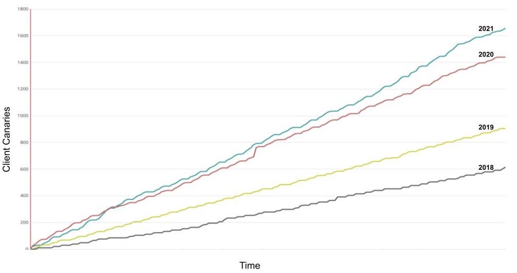
Today, most client applications at Netflix use the client canary model to continuously update their applications. We have seen a significant increase in adoption of this methodology over the past 4 years as shown in this cumulative graph of client canary counts.

Year-over-year increase in Client Canaries at Netflix

Time constraints, the need for speed and quality have created several challenges in the client application’s frequent update domain that our team at Netflix aims to solve. We covered some metric related ones in a previous post describing “How Netflix uses Druid for Real-time Insights to Ensure a High-Quality Experience”. We intend to share more in the future diving into the challenges and solutions in the Allocation, Analysis and Orchestration space.

Safe Updates of Client Applications at Netflix was originally published in Netflix TechBlog on Medium, where people are continuing the conversation by highlighting and responding to this story.

In a win for the Internet, federal court rejects copyright infringement claim against Cloudflare

2021-10-07 Patrick Nemeroff

Post Syndicated from Patrick Nemeroff original https://blog.cloudflare.com/in-a-win-for-the-internet-federal-court-rejects-copyright-infringement-claim-against-cloudflare/

In a win for the Internet, federal court rejects copyright infringement claim against Cloudflare

Since the founding of the Internet, online copyright infringement has been a real concern for policy makers, copyright holders, and service providers, and there have been considerable efforts to find effective ways to combat it. Many of the most significant legal questions around what is called “intermediary liability” — the extent to which different links in the chain of an Internet transmission can be held liable for problematic online content — have been pressed on lawmakers and regulators, and played out in courts around issues of copyright.

Although section 230 of the Communications Decency Act in the United States provides important protections from liability for intermediaries, copyright and other intellectual property claims are one of the very few areas carved out of that immunity.

A Novel Theory of Liability

Over the years, copyright holders have sometimes sought to hold Cloudflare liable for infringing content on websites using our services. This never made much sense to us. We don’t host the content of the websites at issue, we don’t aggregate or promote the content or in any way help end users find it, and our services are not even necessary for the content’s availability online. Infrastructure service providers like Cloudflare are not well positioned to solve problems like online infringement.

Also, while we cannot prevent online infringement, we’ve set up abuse processes to assist copyright holders address the issue by connecting them with the hosting providers and website operators actually able to take such content off the Internet.

But the combination of decades-old copyright statutes and rapidly innovating Internet services has left some copyright holders believing they might have a viable claim against us. Add in the fact that statutory damage provisions in the United States copyright law were not written with the Internet in mind and seemingly allow for the possibility of astronomical damage awards when content is transmitted online at scale. So it’s not altogether surprising that plaintiffs are sometimes tempted to try their luck suing Cloudflare.

A Novel Theory Rejected

Yesterday, in Mon Cheri Bridals, LLC v. Cloudflare, Inc., the United States District Court for the Northern District of California rejected one such lawsuit, granting Cloudflare’s motion for summary judgment and concluding that no reasonable jury could find Cloudflare liable for the alleged copyright infringement at issue.

The plaintiffs in the case sell wedding dresses online, and they asserted that other websites illegally used their copyrighted pictures of the dresses while selling knockoff dresses. In a quirk of US copyright law, most fashion designs are not copyright protected, while pictures of those designs can be protected. Rather than pursue their claims against the website operators, their hosting providers, or any of the numerous other service providers necessary to their business, the plaintiffs targeted Cloudflare, seeking to hold us liable for contributory copyright infringement on the grounds that the websites at issue used our CDN and pass-through security services, most of them for free.

The district court rejected that claim, holding that merely providing CDN and pass-through security services to the websites did not make Cloudflare responsible for their alleged infringement. The court explained that Cloudflare’s services were not necessary to and did not “significantly magnify” any infringement. It also recognized that Cloudflare cannot eliminate infringement by websites using its CDN services, because “removing material from a cache without removing it from the hosting service would not prevent the direct infringement from occurring.” Finally, the court observed that Cloudflare’s abuse reporting system is designed to put copyright holders in the same position they would be if the websites at issue were not using our services, by connecting copyright holders with the hosting providers and website operators actually able to effectively address the issue. Notably, the court decided the case solely on the contributory infringement issue, and it did not even reach our independent arguments that we are protected from any liability by the Digital Millennium Copyright Act’s safe harbors.

Moving forward with clarity

Obviously, we agree with the district court’s reasoning, and we hope it goes a long way towards discouraging these types of claims in the future. Throughout this case, we’ve worked closely with our attorneys at Fenwick & West who have demonstrated great skill and diligence. We plan to continue to fight other lawsuits of this nature. We have long understood that different types of services have different abilities and responsibilities to address online infringement, and we designed our abuse process with that in mind. Broader recognition of those principles will allow us to “help build a better Internet” by providing security and reliability services without being dragged into every dispute between third parties and someone who uses our services. We think that will be better for the Internet.

Update the alternate security contact across your AWS accounts for timely security notifications

2021-10-07 Steven Bedeker

Post Syndicated from Steven Bedeker original https://aws.amazon.com/blogs/security/update-the-alternate-security-contact-across-your-aws-accounts-for-timely-security-notifications/

Amazon Web Services (AWS) will send you important security notifications from time to time related to your account. From a security perspective, the ability for AWS Security to reach you in a timely manner is important whether you have one AWS account or thousands. These notifications could include alerts from AWS Security for potentially fraudulent activity on your AWS account or other messages from AWS Support and service teams regarding security-related topics associated with AWS account usage. This is why we added the alternate security contact—an additional contact field within AWS accounts that you can use to ensure that the right people are notified at the right time.

Make sure you get these notifications in a timely manner by confirming that the contact details on your accounts—especially the security contacts—are accurate and routed to an email account that is regularly monitored. If you have multiple accounts, several teams might need to be notified in the event of a security issue. This could be the account owner, platform teams, and security teams who need to work together to investigate the issue. Contacting only the primary account holder email isn’t always sufficient, particularly in time-sensitive situations. Larger organizations with decentralized development teams—but with a centralized security or governance function—may need to notify a non-technical primary account holder, who might be a business owner with little insight into the workloads within the account. Using a centralized security contact email address for multiple accounts that points to a shared inbox or a distribution list is typically the best practice. Providing additional contact details so that AWS can alert multiple contacts gives centralized teams a better view of decentralized environments, while also reducing the risk of a bottleneck in communications from AWS.

Note: Although AWS Organizations enables many aspects of account management to be done centrally, notifications typically are performed on a per-account basis. To update your account details across multiple accounts, try the new API for programmatically managing alternate contacts on member accounts with AWS Organizations.

Consider the challenges faced by a central security team for a large, diversified corporation; or for a large government agency with a wide range of sub-agencies, contractors, or resellers running workloads on their behalf. The primary account holder might be several steps removed from the central security team. In these cases, and particularly with contractors or resellers, these groups might not be part of the same AWS Organizations account. Having a single security contact email address in all the relevant AWS accounts gives the central security team a way to be notified of issues in these accounts.

To create better security communications with our customers, AWS has modified our internal systems and practices to send security-related email notifications to both the primary account holder as well as the alternate security contact (if provided). In some cases, what you have entered in the alternate security contact full name field will also be included in this email outreach. You can use the full name field to provide useful context regarding the account to help expedite investigation and remediation by a central security team. As a best practice, don’t include sensitive information in the full name field.

Conclusion

Make sure that the primary and alternate account contact details are set up for the workload owners and any additional teams that need to see security notifications. Pay special attention to accurate information for the security contact because AWS will use that email address for security-related outbound notifications. Centralize those security notifications where appropriate by using a common shared inbox or distribution list across multiple AWS accounts. Account management information can be found at Managing an AWS account. You can use the newly launched account management API for programmatically monitoring and updating as appropriate the alternate contacts on individual accounts or on member accounts with AWS Organizations.

If you have feedback about this post, submit comments in the Comments section below.

Using Okta as an identity provider with Amazon MWAA

2021-10-07 James Beswick

Post Syndicated from James Beswick original https://aws.amazon.com/blogs/compute/using-okta-as-an-identity-provider-with-amazon-mwaa/

This post is written by Henry Robalino, Solutions Architect.

Amazon Managed Workflows for Apache Airflow (Amazon MWAA), is a fully managed service that allows data engineers and data scientists to run data processing workflows in the cloud. Okta is a third-party identity provider (IdP) that allows customers to use AWS Single Sign-On (AWS SSO) for their employees to be able to log in quickly and securely.

This blog post shows how to integrate Okta with AWS SSO to access Amazon MWAA using single sign-on.

Overview

Customers use Amazon MWAA to run workflows at scale on the cloud. They want to use their existing login solutions and investments the business made on their current IdP, in this case Okta.

AWS SSO does not yet provide APIs to automate creation and configuration of custom SAML 2.0 applications. As a result, many of the steps in this blog are manual and require using the AWS Management Console.

Prerequisites

Deploying this solution requires:

Okta:
- Okta account
- Okta user account to be used with Amazon MWAA
AWS Identity and Access Management (IAM):
- IAM account with proper permissions to edit AWS SSO
AWS SSO:
Amazon MWAA:
- Amazon MWAA environment deployed
- Amazon MWAA web UI URL

Creating an Amazon MWAA application in AWS SSO

Create a custom SAML 2.0 application for Amazon MWAA

Sign into the AWS Management Console, using an account with the appropriate permissions to modify AWS SSO.
In the AWS SSO console, navigate to Applications. Select “Add a new application”.
On the Add New Application page, select “Add a custom SAML 2.0 application”:
On the Configure Custom SAML 2.0 application:
1. For Display name, enter AWS_SSO_Amazon_MWAA.
2. For Description, enter AWS SSO Application for Amazon MWAA.
In the Application metadata section, select the option to manually type in the metadata values.
Before:

After:
Enter the Application properties and Application metadata sections:
- Application start URL: This is the Amazon MWAA WebLogin URL, which you can locate in the Amazon MWAA console.
  - For example: https://123456a0-0101-2020-9e11-1b159eec9000.c2.us-east-1.airflow.amazonaws.com
- Application ACS URL: This is the Assertion Consumer Service (ACS) URL that AWS SSO provides.
  - For example: https://us-east-1.signin.aws.amazon.com/platform/saml/acs/012345678-0102-0304-0506-EXAMPLE01
- Application SAML audience: This is the SAML audience that AWS SSO provides.
  - For example: https://us-east-1.signin.aws.amazon.com/platform/saml/d-012345678E
The Application properties and Application metadata now look like this:
Choose Save changes. A custom SAML 2.0 application for Amazon MWAA is created. You are now redirected to the AWS_SSO_Amazon_MWAA application page.
On the Attribute mappings tab, modify the existing Subject attribute to “${user:subject}” and a Format of “unspecified.” Choose Save changes.
On the Assigned users tab, add the previously created Amazon MWAA Okta user. Select Assign users and the user. Choose Save changes.

You have now created a custom application for Amazon MWAA in AWS SSO. You have added a user and configured the attribute mappings.

Configuring an Amazon MWAA Permission Sets in AWS SSO

Assign IAM permissions to the newly created Amazon MWAA application by using a permissions set. A permission set is a collection of administrator-defined policies that AWS SSO uses to determine a user’s effective permissions to access a given AWS account.

Navigate to the AWS SSO console. Select on AWS accounts on the left-hand side. Select the Permission sets tab and choose the Create permission set button.
Select the Create a custom permission set option.
Provide a name for the Custom Permission Set and an optional description. Choose the Create a custom permissions policy check box.

In the new text field, add the IAM policy below. This set of permissions is associated with the AWS_SSO_Amazon_MWAA application. Make sure to use the correct Amazon Resource Names (ARN) for your Amazon MWAA environment in the below sample text.Sample IAM policy:

{
    "Version": "2012-10-17",
    "Statement": [
        {
            "Effect": "Allow",
            "Action": [
                "airflow:GetEnvironment",
                "airflow:CreateCliToken"
            ],
            "Resource": "arn:aws:airflow:us-east-1:111222333444:environment/MY-MWAA-ENV"
        },
        {
            "Effect": "Allow",
            "Action": "airflow:CreateWebLoginToken",
            "Resource": "arn:aws:airflow:us-east-1:111222333444:role/MY-MWAA-ENV/viewer"
        }
    ]
}

The policy enables the following permissions:

- GetEnvironment – retrieves the details of an Amazon MWAA environment
- CreateCLIToken – creates a CLI token request for an MWAA environment.
- CreateWebLoginToken – creates an Airflow web UI login token request for the Amazon MWAA environment.
  - /viewer – level of access for the user of the web token, see Apache Airflow roles.

5. Follow the prompts to fill out tags as necessary. Choose Proceed to AWS accounts.

You have now finished configuring the Amazon MWAA application inside of AWS SSO.

Testing and validation

To test and validate the configuration:

Navigate to your Okta SSO portal. Sign in with the appropriate account that is assigned to the Amazon MWAA application.
To access Amazon MWAA, select the AWS Account application. This opens up the AWS Management Console in another window. Once this window opens, close it. As of this writing Amazon MWAA does not support “Auth Mode: SSO”, hence this workaround.
Next, select the AWS_SSO_Amazon_MWAA application. You are redirected to the Amazon MWAA SSO Page.
Choose the Sign in with AWS Management Console SSO.
You are redirected to the Amazon MWAA web server UI.

In this page, you can see all the DAGs available to you and view the DAG history. In the top-right corner, you can see that you are logged in using the AWS SSO assumed role.

Conclusion

This blog post shows you how to integrate Amazon MWAA with Okta as your managed AWS SSO implementation. You can use this solution for your own use cases and enable Okta SSO and Amazon MWAA.

To stay up to date with AWS Identity launches, see: https://aws.amazon.com/blogs/security/highlights-from-the-latest-aws-identity-launches/.

For more serverless learning resources, visit Serverless Land.

Interpreting A/B test results: false positives and statistical significance

2021-10-07 Netflix Technology Blog

Post Syndicated from Netflix Technology Blog original https://netflixtechblog.com/interpreting-a-b-test-results-false-positives-and-statistical-significance-c1522d0db27a

Martin Tingley with Wenjing Zheng, Simon Ejdemyr, Stephanie Lane, and Colin McFarland

This is the third post in a multi-part series on how Netflix uses A/B tests to inform decisions and continuously innovate on our products. Need to catch up? Have a look at Part 1 (Decision Making at Netflix) and Part 2 (What is an A/B Test?). Subsequent posts will go into more details on experimentation across Netflix, how Netflix has invested in infrastructure to support and scale experimentation, and the importance of the culture of experimentation within Netflix.

In Part 2: What is an A/B Test we talked about testing the Top 10 lists on Netflix, and how the primary decision metric for this test was a measure of member satisfaction with Netflix. If a test like this shows a statistically significant improvement in the primary decision metric, the feature is a strong candidate for a roll out to all of our members. But how do we know if we’ve made the right decision, given the results of the test? It’s important to acknowledge that no approach to decision making can entirely eliminate uncertainty and the possibility of making mistakes. Using a framework based on hypothesis generation, A/B testing, and statistical analysis allows us to carefully quantify uncertainties, and understand the probabilities of making different types of mistakes.

There are two types of mistakes we can make in acting on test results. A false positive (also called a Type I error) occurs when the data from the test indicates a meaningful difference between the control and treatment experiences, but in truth there is no difference. This scenario is like having a medical test come back as positive for a disease when you are healthy. The other error we can make in deciding on a test is a false negative (also called a Type II error), which occurs when the data do not indicate a meaningful difference between treatment and control, but in truth there is a difference. This scenario is like having a medical test come back negative — when you do indeed have the disease you are being tested for.

As another way to build intuition, consider the real reason that the internet and machine learning exist: to label if images show cats. For a given image, there are two possible decisions (apply the label “cat” or “not cat”), and likewise there are two possible truths (the image either features a cat or it does not). This leads to a total of four possible outcomes, shown in Figure 1. The same is true with A/B tests: we make one of two decisions based on the data (“sufficient evidence to conclude that the Top 10 list affects member satisfaction” or “insufficient evidence”), and there are two possible truths, that we never get to know with complete uncertainty (“Top 10 list truly affects member satisfaction” or “it does not”).

Figure 1: The four possible outcomes when labeling an image as either showing a cat or not.

The uncomfortable truth about false positives and false negatives is that we can’t make them both go away. In fact, they trade off with one another. Designing experiments so that the rate of false positives is minuscule necessarily increases the false negative rate, and vice versa. In practice, we aim to quantify, understand, and control these two sources of error.

In the remainder of this post, we’ll use simple examples to build up intuition around false positives and related statistical concepts; in the next post in this series, we’ll do the same for false negatives.

False positives and statistical significance

With a great hypothesis and a clear understanding of the primary decision metric, it’s time to turn to the statistical aspects of designing an A/B test. This process generally starts by fixing the acceptable false positive rate. By convention, this false positive rate is usually set to 5%: for tests where there is not a meaningful difference between treatment and control, we’ll falsely conclude that there is a “statistically significant” difference 5% of the time. Tests that are conducted with this 5% false positive rate are said to be run at the 5% significance level.

Using the 5% significance level convention can feel uncomfortable. By following this convention, we are accepting that, in instances when the treatment and control experience are not meaningfully different for our members, we’ll make a mistake 5% of the time. We’ll label 5% of the non-cat photos as displaying cats.

The false positive rate is closely associated with the “statistical significance” of the observed difference in metric values between the treatment and control groups, which we measure using the p-value. The p-value is the probability of seeing an outcome at least as extreme as our A/B test result, had there truly been no difference between the treatment and control experiences. An intuitive way to understand statistical significance and p-values, which have been confusing students of statistics for over a century (your authors included!), is in terms of simple games of chance where we can calculate and visualize all the relevant probabilities.

Figure 2: Thinking about simple games of chance, such as flipping coins like this one displaying Julius Caesar, is a great way to build up intuition about statistics.

Say we want to know if a coin is unfair, in the sense that the probability of heads is not 0.5 (or 50%). It may sound like a simple scenario, but it is directly relevant to many businesses, Netflix included, where the goal is to understand if a new product experience results in a different rate for some binary user activity, from clicking on a UI feature to retaining the Netflix service for another month. So any intuition we can build through simple games with coins maps directly to interpreting A/B tests.

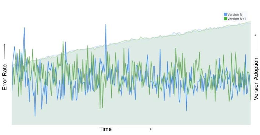
To decide if the coin is unfair, let’s run the following experiment: we’ll flip the coin 100 times and calculate the fraction of outcomes that are heads. Because of randomness, or “noise,” even if the coin were perfectly fair we wouldn’t expect exactly 50 heads and 50 tails — but how much of a deviation from 50 is “too much”? When do we have sufficient evidence to reject the baseline assertion that the coin is in fact fair? Would you be willing to conclude that the coin is unfair if 60 out of 100 flips were heads? 70? We need a way to align on a decision framework and understand the associated false positive rate.

To build intuition, let’s run through a thought exercise. First, we’ll assume the coin is fair — this is our “null hypothesis,” which is always a statement of status quo or equality. We then seek compelling evidence against this null hypothesis from the data. To make a decision on what constitutes compelling evidence, we calculate the probability of every possible outcome, assuming that the null hypothesis is true. For the coin flipping example, that’s the probability of 100 flips yielding zero heads, one head, two heads, and so forth up to 100 heads — assuming that the coin is fair. Skipping over the math, each of these possible outcomes and their associated probabilities are shown with the black and blue bars in Figure 3 (ignore the colors for now).

We can then compare this probability distribution of outcomes, calculated under the assumption that the coin is fair, to the data we’ve collected. Say we observe that 55% of 100 flips are heads (the solid red line in Figure 3). To quantify if this observation is compelling evidence that the coin is not fair, we count up the probabilities associated with every outcome that is less likely than our observation. Here, because we’ve made no assumptions about heads or tails being more likely, we sum up the probabilities of 55% or more of the flips coming up heads (the bars to the right of the solid red line) and the probabilities of 55% or more of the flips coming up tails (the bars to the left of the dashed red line).

This is the mythical p-value: the probability of seeing a result as extreme as our observation, if the null hypothesis were true. In our case, the null hypothesis is that the coin is fair, the observation is 55% heads in 100 flips, and the p-value is about 0.32. The interpretation is as follows: were we to repeat, many times, the experiment of flipping a coin 100 times and calculating the fraction of heads, with a fair coin (the null hypothesis is true), in 32% of those experiments the outcome would feature at least 55% heads or at least 55% tails (results at least as unlikely as our actual observation).

Figure 3: Flipping a fair coin 100 times, the probability of each outcome expressed as the fraction of heads.

How do we use the p-value to decide if there is statistically significant evidence that the coin is unfair — or that our new product experience is an improvement on the status quo? It comes back to that 5% false positive rate that we agreed to accept at the beginning: we conclude that there is a statistically significant effect if the p-value is less than 0.05. This formalizes the intuition that we should reject the null hypothesis that the coin is fair if our result is sufficiently unlikely to occur under the assumption of a fair coin. In the example of observing 55 heads in 100 coin flips, we calculated a p-value of 0.32. Because the p-value is larger than the 0.05 significance level, we conclude that there is not statistically significant evidence that the coin is unfair.

There are two conclusions that we can make from an experiment or A/B test: we either conclude there is an effect (“the coin is unfair”, “the Top 10 feature increases member satisfaction”) or we conclude that there is insufficient evidence to conclude there is an effect (“cannot conclude the coin is unfair,” “cannot conclude that the Top 10 row increases member satisfaction”). It’s a lot like a jury trial, where the two possible outcomes are “guilty” or “not guilty” — and “not guilty” is very different from “innocent.” Likewise, this (frequentist) approach to A/B testing does not allow us to make the conclusion that there is no effect — we never conclude the coin is fair, or that the new product feature has no impact on our members. We just conclude we’ve not collected enough evidence to reject the null assumption that there is no difference. In the coin example above, we observed 55% heads in 100 flips, and concluded we had insufficient evidence to label the coin as unfair. Critically, we did not conclude that the coin was fair — after all, if we gathered more evidence, say by flipping that same coin 1000 times, we might find sufficiently compelling evidence to reject the null hypothesis of fairness.

Rejection Regions and Confidence Intervals

There are two other concepts in A/B testing that are closely related to p-values: the rejection region for a test, and the confidence interval for an observation. We cover them both in this section, building on the coin example from above.

Rejection Regions. Another way to build a decision rule for a test is in terms of what’s called a “rejection region” — the set of values for which we’d conclude that the coin is unfair. To calculate the rejection region, we once more assume the null hypothesis is true (the coin is fair), and then define the rejection region as the set of least likely outcomes with probabilities that sum to no more than 0.05. The rejection region consists of the outcomes that are the most extreme, provided the null hypothesis is correct — the outcomes where the evidence against the null hypothesis is strongest. If an observation falls in the rejection region, we conclude that there is statistically significant evidence that the coin is not fair, and “reject” the null. In the case of the simple coin experiment, the rejection region corresponds to observing fewer than 40% or more than 60% heads (shown with blue shaded bars in Figure 3). We call the boundaries of the rejection region, here 40% and 60% heads, the critical values of the test.

There is an equivalence between the rejection region and the p-value, and both lead to the same decision: the p-value is less than 0.05 if and only if the observation lies in the rejection region.

Confidence Intervals. So far, we’ve approached building a decision rule by first starting with the null hypothesis, which is always a statement of no change or equivalence (“the coin is fair” or “the product innovation does not impact member satisfaction”). We then define possible outcomes under this null hypothesis and compare our observation to that distribution. To understand confidence intervals, it helps to flip the problem around to focus on the observation. We then go through a thought exercise: given the observation, what values of the null hypothesis would lead to a decision not to reject, assuming we specify a 5% false positive rate? For our coin flipping example, the observation is 55% heads in 100 flips and we do not reject the null of a fair coin. Nor would we reject the null hypothesis that the probability of heads was 47.5%, 50%, or 60%. There’s a whole range of values for which we would not reject the null, from about 45% to 65% probability of heads (Figure 4).

This range of values is a confidence interval: the set of values under the null hypothesis that would not result in a rejection, given the data from the test. Because we’ve mapped out the interval using tests at the 5% significance level, we’ve created a 95% confidence interval. The interpretation is that, under repeated experiments, the confidence intervals will cover the true value (here, the actual probability of heads) 95% of the time.

There is an equivalence between the confidence interval and the p-value, and both lead to the same decision: the 95% confidence interval does not cover the null value if and only if the p-value is less than 0.05, and in both cases we reject the null hypothesis of no effect.

Figure 4: Building the confidence interval by mapping out the set of values that, when used to define a null hypothesis, would not result in rejection for a given observation.

Summary

Using a series of thought exercises based on flipping coins, we’ve built up intuition about false positives, statistical significance and p-values, rejection regions, confidence intervals, and the two decisions we can make based on test data. These core concepts and intuition map directly to comparing treatment and control experiences in an A/B test. We define a “null hypothesis” of no difference: the “B” experience does not alter affect member satisfaction. We then play the same thought experiment: what are the possible outcomes and their associated probabilities for the difference in metric values between the treatment and control groups, assuming there is no difference in member satisfaction? We can then compare the observation from the experiment to this distribution, just like with the coin example, calculate a p-value and make a conclusion about the test. And just like with the coin example, we can define rejection regions and calculate confidence intervals.

But false positives are only of the two mistakes we can make when acting on test results. In the next post in this series, we’ll cover the other type of mistake, false negatives, and the closely related concept of statistical power. Follow the Netflix Tech Blog to stay up to date.

Interpreting A/B test results: false positives and statistical significance was originally published in Netflix TechBlog on Medium, where people are continuing the conversation by highlighting and responding to this story.

1.1.1.1

Impact on other sites

Attacks

Network Error Logs

WARP

Our own traffic

Core Web Vitals

Conclusion

Apple Silicon support on the Insight Agent

Asset and Vulnerability Details reports

Snyk integration for reporting vulnerabilities

Emergent threat coverage recap

Stay tuned!

NEVER MISS A BLOG

How the vulnerability works

Exploit Attempts

Conclusion

CDK Aspects

How to align with or check configuration compliance using CDK Aspects

Conclusion

About the Authors

Solution Overview

Prerequisites

Create the Artifacts S3 Bucket

Create the AWS CodeBuild Project

Run the Artifacts

Cleaning up

Conclusion

Overview of solution

Architecture overview

Prerequisites

Create the required infrastructure using AWS CloudFormation

Source data and script files S3 bucket

DataBrew dataset, project, recipe, and job

AWS Glue ETL job

Start the Step Function state machine

Run an AWS Glue crawler to create tables in the Data Catalog

Use Athena to run analytics queries

Visualize the processed data on a QuickSight dashboard

Clean up

Conclusion

Appendix A

Appendix B

Appendix C

Appendix D

About the Authors

Client Applications

Deployment Strategies

AB Tests/Client Canaries

Allocation

Metrics

Analysis

Orchestration

Conclusion

A Novel Theory of Liability

A Novel Theory Rejected

Moving forward with clarity

Conclusion

Overview

Prerequisites

Creating an Amazon MWAA application in AWS SSO

Create a custom SAML 2.0 application for Amazon MWAA

Configuring an Amazon MWAA Permission Sets in AWS SSO

Testing and validation

Conclusion

False positives and statistical significance

​​Rejection Regions and Confidence Intervals

Summary

The collective thoughts of the interwebz

Rejection Regions and Confidence Intervals