Waiting Room: Random Queueing and Custom Web/Mobile Apps

Post Syndicated from Tyler Caslin original https://blog.cloudflare.com/waiting-room-random-queueing-and-custom-web-mobile-apps/


Waiting Room: Random Queueing and Custom Web/Mobile Apps

Waiting Room: Random Queueing and Custom Web/Mobile Apps

Today, we are announcing the general availability of Cloudflare Waiting Room to customers on our Enterprise plans, making it easier than ever to protect your website against traffic spikes. We are also excited to present several new features that have user experience in mind — an alternative queueing method and support for custom web/mobile applications.

First-In-First-Out (FIFO) Queueing
Waiting Room: Random Queueing and Custom Web/Mobile Apps

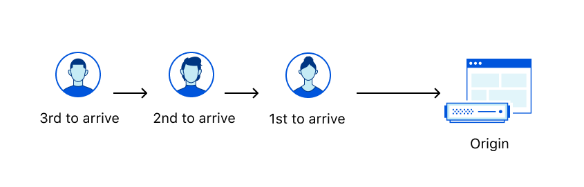
Whether you’ve waited to check out at a supermarket or stood in line at a bank, you’ve undoubtedly experienced FIFO queueing. FIFO stands for First-In-First-Out, which simply means that people are seen in the order they arrive — i.e., those who arrive first are processed before those who arrive later.

When Waiting Room was introduced earlier this year, it was first deployed to protect COVID-19 vaccine distributors from overwhelming demand — a service we offer free of charge under Project Fair Shot. At the time, FIFO queueing was the natural option due to its wide acceptance in day-to-day life and accurate estimated wait times. One problem with FIFO is that users who arrive later could see long estimated wait times and decide to abandon the website.

We take customer feedback seriously and improve products based on it. A frequent request was to handle users irrespective of the time they arrive in the Waiting Room. In response, we developed an additional approach: random queueing.

A New Approach to Fairness: Random Queueing
Waiting Room: Random Queueing and Custom Web/Mobile Apps

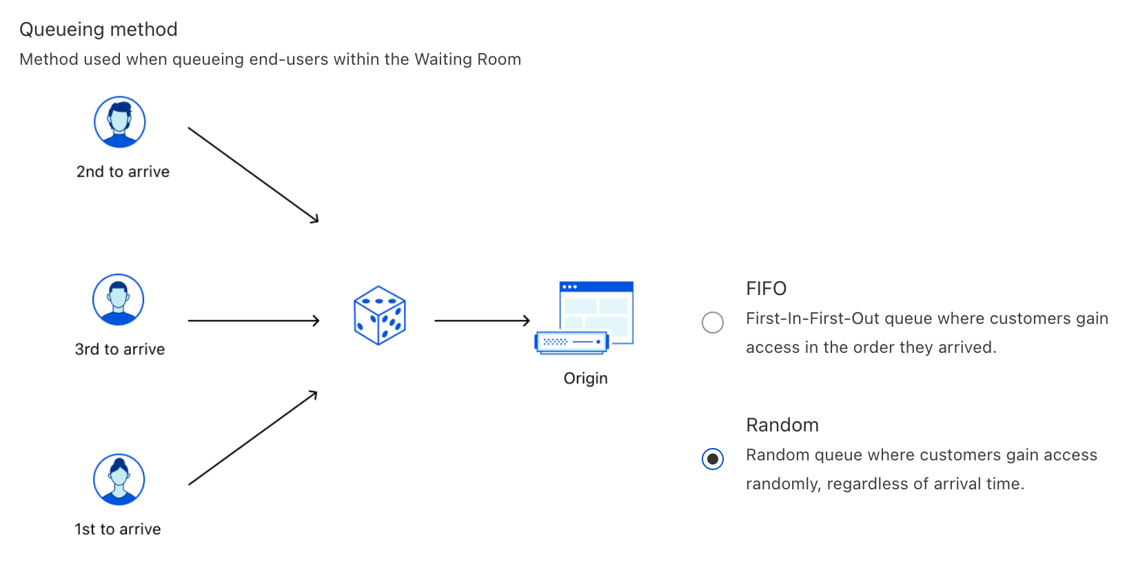
You can think of random queueing as participating in a raffle for a prize. In a raffle, people obtain tickets and put them into a big container. Later, tickets are drawn at random to determine the winners. The more time you spend in the raffle, the better your chances of winning at least once, since there will be fewer tickets in the container. No matter what, everyone participating in the raffle has an opportunity to win.

Similarly, in a random queue, users are selected from the Waiting Room at random, regardless of their initial arrival time. This means that you could be let into the application before someone who arrived earlier than you, or vice versa. Just like how you can buy more tickets in a raffle, joining a random queue earlier than someone else will give you more attempts to be accepted, but does not guarantee you will be let in. However, at any particular time, you will have the same chance to be let into the website as anyone else. This is different from a raffle, where you could have more tickets than someone else at a given time, providing you with an advantage.

Random queueing is designed to give everyone a fair chance. Imagine waking up excited to purchase new limited-edition sneakers only to find that the FIFO queue is five hours long and full of users that either woke up in the middle of the night to get in line or joined from earlier time zones. Even if you waited five hours, those sneakers would likely be sold out by the time you reach the website. In this case, you’d probably abandon the Waiting Room completely and do something else. On the other hand, if you were aware that the queue was random, you’d likely stick around. After all, you have a chance to be accepted and make a purchase!

As a result, random queueing is perfect for short-lived scenarios with lots of hype, such as product launches, holiday traffic, special events, and limited-time sales.

By contrast, when the event ends and traffic returns to normal, a FIFO queue is likely more suitable, since its widely accepted structure and accurate estimated wait times provide a consistent user experience.

How Does Random Queueing Work?
Waiting Room: Random Queueing and Custom Web/Mobile Apps

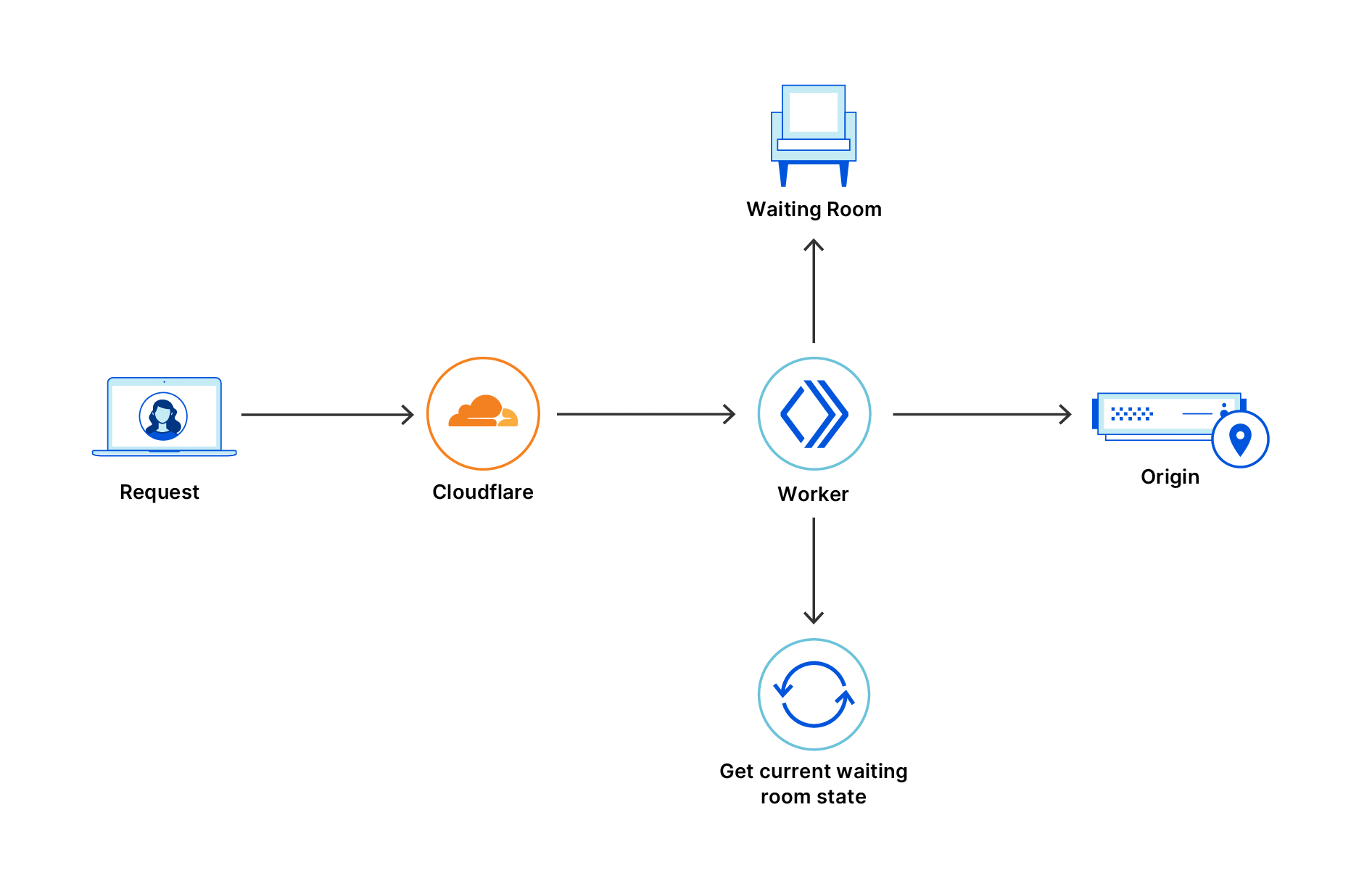
Perhaps the best part about random queueing is that it maintains the same internal structure that powers FIFO. As a result, if you change the queueing method in the dashboard — even when you may be actively queueing users — the transition to the new method is seamless. Imagine you have users 1, 2, 3, 4, and 5 waiting in a FIFO queue in the order 5 →  4 → 3 → 2 → 1, where user 1 will be the next user to access the application. Let’s assume you switch to random queueing. Now, any user can be accepted next. Let’s assume user 4 is accepted. If you decide to immediately switch back to FIFO queueing, the queue will reflect the order 5 → 3 → 2 → 1. In other words, transitioning from FIFO to random and back to FIFO will respect the initial queue positions of the users! But how does this work? To understand, we first need to remember how we built Waiting Room for FIFO.

Recall the Waiting Room configurations:

  • Total Active Users. The total number of active users that can be using the application at any given time.
  • New Users Per Minute. The maximum number of new users per minute that can be accepted to the application.

Next, remember that Waiting Room is powered by cookies. When you join the Waiting Room for the first time, you are assigned an encrypted cookie. You bring this cookie back to the Waiting Room and update it with every request, using it to prove your initial arrival time and status.

Properties in the Waiting Room cookie include:

  • bucketId. The timestamp rounded down to the nearest minute of the user’s first request to the Waiting Room. If you arrive at 10:23:45, you will be grouped into a bucket for 10:23:00.
  • acceptedAt. The timestamp when the user got accepted to the origin website for the first time.
  • refreshIntervalSeconds. When queueing, this is the number of seconds the user must wait before sending another request to the Waiting Room.
  • lastCheckInTime. The last time each user checked into the Waiting Room or origin website. When queueing, this is only updated for requests every refreshIntervalSeconds.

For any given minute, we can calculate the number of users we can let into the origin website. Let’s say we deploy a Waiting Room on “https://example.com/waitingroom” that can support 10,000 Total Active Users, and we allow up to 2,000 New Users Per Minute. If there are currently 7,000 active users on the website, we have 10,000 – 7,000 = 3,000 open slots. However, we need to take the minimum (3,000, 2,000) = 2,000 since we need to respect the New Users Per Minute limit. Thus, we have 2,000 available slots we can give out.

Let’s assume there are 2,500 queued users that joined over the last three minutes in groups of 500, 1,000, and 1,000, respectively for the timestamps 15:54, 15:55, and 15:56. To respect FIFO queueing, we will take our 2,000 available slots and try to reserve them for users who joined first. Thus, we will reserve 500 available slots for the users who joined at 15:54 and then reserve 1000 available slots for the users who joined at 15:55. When we get to the users for 15:56, we see that we only have 500 slots left, which is not enough for the 1,000 queued users for this minute:

{
	"activeUsers": 7000,
	"buckets": [{
			"key": "Thu, 27 May 2021 15:54:00 GMT",
			"data": {
				"waiting": 500,
				"reservedSlots": 500
			}
		},
		{
			"key": "Thu, 27 May 2021 15:55:00 GMT",
			"data": {
				"waiting": 1000,
				"reservedSlots": 1000
			}
		},
		{
			"key": "Thu, 27 May 2021 15:56:00 GMT",
			"data": {
				"waiting": 1000,
				"reservedSlots": 500
			}
		}
	]
}

Since we have reserved slots for all users with bucketIds of 15:54 and 15:55, they can be let into the origin website from any data center. However, we can only let in a subset of the users who initially arrived at 15:56.

Timestamp (bucketId) Queued Users Reserved Slots Strategy
15:54 500 500 Accept all users
15:55 1,000 1,000 Accept all users
15:56 1,000 500 Accept subset of users

These 500 slots for 15:56 are allocated to each Cloudflare edge data center based on its respective historical traffic data, and further divided for each Cloudflare Worker within the data center. For example, let’s assume there are two data centers — Nairobi and Dublin — which share 60% and 40% of the traffic, respectively, for this minute. In this case, we will allocate 500 * .6 = 300 slots for Nairobi and 500 * .4 = 200 slots for Dublin. In Nairobi, let’s say there are 3 active workers, so we will grant each of them 300 / 3 = 100 slots. If you make a request to a worker in Nairobi and your bucketId is 15:56, you will be allowed in and consume a slot if the worker still has at least one of its 100 slots available. Since we have reserved all 2,000 available slots, users with bucketIds after 15:56 will have to continue queueing.

Let’s modify this case and assume we only have 200 queued users, all of which are in the 15:54 bucket. First, we reserve 200 slots for these queued users, leaving us 2,000 – 200 = 1,800 remaining slots. Since we have reserved slots for all queued users, we can use the remaining 1,800 slots on new users — people who have just made their first request to the Waiting Room and don’t have a cookie or bucketId yet. Similar to how we handle buckets with fewer slots than queued users, we will distribute these 1,800 slots to each data center, allocating 1,800 * .6 = 1,080 to Nairobi and 1,800 * .4 = 720 to Dublin. In Nairobi, we will split these equally across the 3 workers, giving them 1,080 / 3 = 360 slots each. If you are a new user making a request to a worker in Nairobi, you will be accepted and take a slot if the worker has at least one of its 360 slots available, otherwise you will be marked as a queued user and enter the Waiting Room.

Now that we have outlined the concepts for FIFO, we can understand how random queueing operates. Simply put, random queueing functions the same way as FIFO, except we pretend that every user is new. In other words, we will not look at reserved slots when making the decision if the user should be let in. Let’s revisit the last case with 200 queued users in the 15:54 bucket and 2,000 available slots. When random queueing, we allocate the full 2,000 slots to new users, meaning Nairobi gets 2,000 * .6 = 1,200 slots and each of its 3 workers gets 1,200 / 3 = 400 slots. No matter how many users are queued or freshly joining the Waiting Room, all of them will have a chance at taking these slots.

Finally, let’s reiterate that we are only pretending that all users are new — we still assign them to bucketIds and reserve slots as if we were FIFO queueing, but simply don’t make any use of this logic while random queueing is active. That way, we can maintain the same FIFO structure while we are random queueing so that if necessary, we can smoothly transition back to FIFO queueing and respect initial user arrival times.

How “Random” is Random Queueing?

Since random queueing is basically a race for available slots, we were concerned that it could be exploited if the available user slots and the queued user check-ins did not occur randomly.

To ensure all queued users can attempt to get into the website at the same rate, we store (in the encrypted cookie) the last time each user checked into the Waiting Room (lastCheckInTime) to prevent them from attempting to gain access to the website until a number of seconds have passed (refreshIntervalSeconds). This means that spamming the page refresh button will not give you an advantage over other queued users! Be patient — the browser will refresh automatically the moment you are eligible for another chance.

Next, let’s imagine five queued users checking into the Waiting Room every refreshIntervalSeconds=30 at approximately the :00 and :30 minute marks. A new queued user joins the Waiting Room and checks in at approximately :15 and :45. If new slots are randomly released, this new user will have about a 50% chance of being selected next, since it monopolizes over the :00-15 and :30-45 ranges. On the other hand, the other five queued users share the :15-30 and :45-00 ranges, giving them about a 50% / 5 = 10% chance each. Let’s consider that new slots are not randomly released and assume they are always released at :59. In this case, the new queued user will have virtually no chance to be selected before the other five queued users because these users will always check in one second later at :00, immediately consuming any newly released slots.

To address this vulnerability, we changed our implementation to ensure that slots are released randomly and encouraged users to check in at random offsets from each other. To help split up users that are checking in at similar times, we vary each user’s refreshIntervalSeconds by a small, pseudo-randomly generated offset for each check-in and store this new refresh interval in the encrypted Waiting Room cookie for validation on the next request. Thus, a user who previously checked in every 30 seconds might now check in after 29 seconds, then 31 seconds, then 27 seconds, and so on — but still averaging a 30-second refresh interval. Over time, these slight check-in variations become significant, spreading out user check-in times and strengthening the randomness of the queue. If you are curious to learn more about the apparent “randomness” behind mixing user check-in intervals, you can think of it as a chaotic system subjected to the butterfly effect.

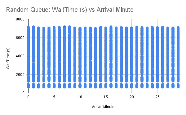
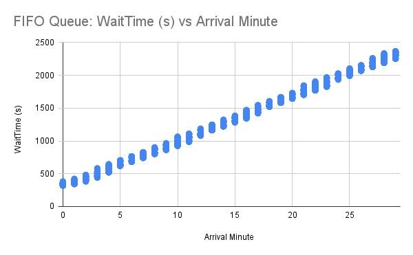
Nevertheless, we weren’t convinced our efforts were enough and wanted to test random queueing empirically to validate its integrity. We conducted a simulation of 10,000 users joining a Waiting Room uniformly across 30 minutes. When let into the application, users spent approximately 1 minute “browsing” before they stopped checking in. We ran this experiment for both FIFO and random queueing and graphed each user’s observed wait time in seconds in the Waiting Room against the minute they initially arrived (starting from 0). Recall that users are grouped by minute using bucketIds, so each user’s arrival minute is truncated down to the current minute.
Waiting Room: Random Queueing and Custom Web/Mobile Apps

Based on our data, we can see immediately for FIFO queueing that, as the arrival minute increases, the observed wait time increases linearly. This makes sense for a FIFO queue, since the “line” will just get longer if there are more users entering the queue than leaving it. For each arrival minute, there is very little variation among user wait times, meaning that if you and your friend join a Waiting Room at approximately the same time, you will both be accepted around the same time. If you join a couple of minutes before your friend, you will almost always be accepted first.

When looking at the results for random queueing, we observe users experiencing varied wait times regardless of the arrival minute. This is expected, and helps prove the “randomness” of the random queue! We can see that, if you join five minutes after your friend, although your friend will have more chances to get in, you may still be accepted first! However, there are so many data points overlapping with each other in the plot that it is hard to tell how they are distributed. For instance, it could be possible that most of these data points experience extreme wait times, but as humans we aren’t able to tell.

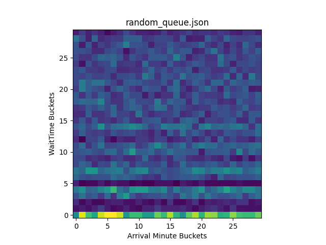
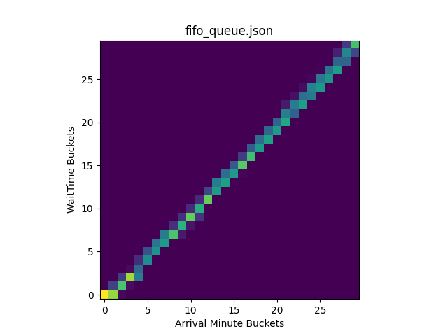
As a result, we created heatmaps of these plots in Python using numpy.histogram2d and displayed them with matplotlib.pyplot:

import json
import numpy as np
import matplotlib.pyplot as plt
import sys
 
filename = sys.argv[1]
 
with open(filename) as file:
   data = json.load(file)
 
   x = data["ArrivalMinutes"]
   y = data["WaitTimeSeconds"]
 
   heatmap, _, _ = np.histogram2d(x, y, bins=(30, 30))
 
   plt.clf()
   plt.title(filename)
   plt.xlabel('Arrival Minute Buckets')
   plt.ylabel('WaitTime Buckets')
   plt.imshow(heatmap.T, origin='lower')
   plt.show()

The heatmaps display where the data points are concentrated in the original plot, using brighter (hotter) colors to represent areas containing more points:
Waiting Room: Random Queueing and Custom Web/Mobile Apps

By inspecting the generated heatmaps, we can conclude that FIFO and random queueing are working properly. For FIFO queueing, users are being accepted in the order they arrive. For random queueing, we can see that users are accepted to the origin regardless of arrival time. Overall, we can see the heatmap for random queueing is well distributed, indicating it is sufficiently random!

If you are curious why random queueing has very hot colors along the lowest wait times followed by very dark colors afterward, it is actually because of how we are simulating the queue. For the simulation, we spoofed the bucketIds of the users and let them all join the Waiting Room at once to see who would be let in first. In the random queueing heatmap, the bright colors along the lowest wait time buckets indicate that many users were accepted quickly after joining the queue across all bucketIds. This is expected, demonstrating that random queueing does not give an edge to users who join earlier, giving each user a fair chance regardless of its bucketId. The reason why these users were almost immediately accepted in WaitTime Bucket 0 is because this simulation started with no users on the origin, meaning new users would be accepted until the Waiting Room limits were reached. Since this first wave of accepted users “browsed” on the origin for a minute before leaving, no additional users during this time were let in. Thus, the colors are very dark for WaitTime Buckets 1 and 2. Similarly, the second wave of users is randomly selected afterward, followed by another period of time when no users were accepted in WaitTime Bucket 5. As the wait time increases, the more attempts a particular user will have to be let in, meaning it is unlikely for users to have extreme wait times. We can see this by observing the colors grow darker as the WaitTime Bucket approaches 29.

How Is Estimated Time Calculated for Random Queueing?

Waiting Room: Random Queueing and Custom Web/Mobile Apps

In a random queue, you can be accepted at any moment… so how can you display an estimated wait time? For a particular user, this is an impossible task, but when you observe all the users together, you can accurately account for most user experiences using a probabilistic estimated wait time range.

At any given moment, we know:

  • letInPerMinute. The current average users per minute being let into the origin.
  • currentlyWaiting. The current number of users waiting in the queue.

Therefore, we can calculate the probability of a user being let into the origin in the next minute:

P(LetInOverMinute) = letInPerMinute / currentlyWaiting

If there are 100 users waiting in the queue, and we are currently letting in 10 users per minute, the probability a user will be let in over the next minute is 10 / 100 = .1 (10%).

Using P(LetInOverMinute), we can determine the n minutes needed for a p chance of being let into the origin:

p = 1 – (1 – P(LetInOverMinute))n

Recall that the probability of getting in at least once is the complement of not getting in at all. The probability of not being let into the origin over n minutes is (1 – P(LetInOverMinutes))n. Therefore, the probability of getting in at least once is 1 – (1 – P(LetInOverMinute))n. This equation can be simplified further:

n = log(1 – p) / log(1 – P(LetInOverMinute))

Thus, if we want to calculate the estimated wait time to have a p = .5 (50%) chance of getting into the origin with the probability of getting let in during a particular minute P(LetInOverMinute) = .1 (10%), we calculate:

n = log(1 – .5) / log(1 – .1) ≈ 6.58 minutes or 6 minutes and 35 seconds

In this case, we estimate that 50% of users will wait less than 6 minutes and 35 seconds and the remaining 50% of users will wait longer than this.

So, which estimated wait times are displayed to the user? It is up to you! If you create a Mustache HTML template for a Waiting Room, you will now be able to use the variables waitTime25Percentile, waitTime50Percentile, and waitTime75Percentile to display the estimated wait times in minutes when p = .25, p = .5, and p = .75, respectively. There are also new variables that are used to display and determine the queueing method, such as queueingMethod, isFIFOQueue, and isRandomQueue. If you want to display something more dynamic like a custom view in a mobile app, keep reading to learn about our new JSON response, which provides a REST API for the same set of variables.

Supporting Dynamic Applications with a JSON Response
Waiting Room: Random Queueing and Custom Web/Mobile Apps

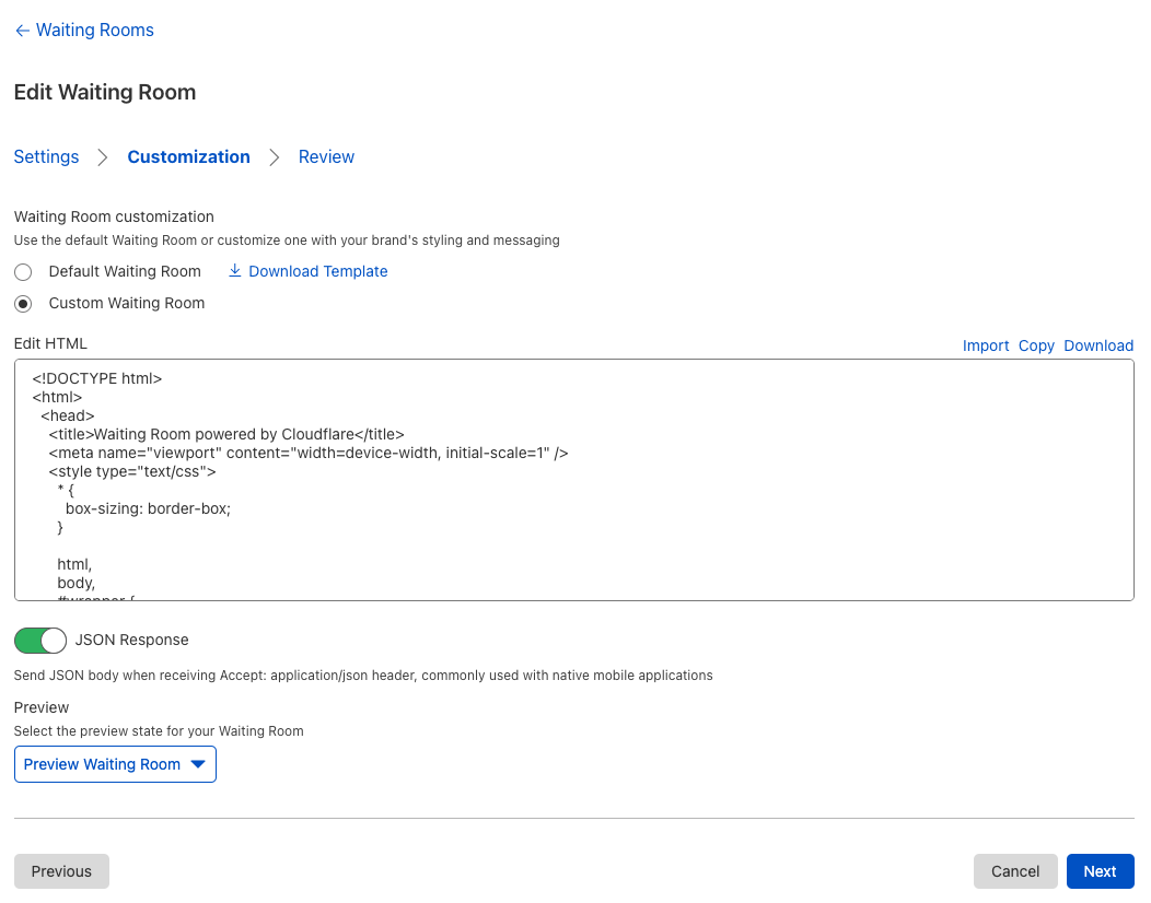
Before, customers could only deploy static Mustache HTML templates to customize the style of their Waiting Rooms. These templates work well for most use cases, but fall short if you want to display anything that requires state. Let’s imagine you’re queueing to buy concert tickets on your mobile device, and you see an embedded video of your favorite song. Naturally, you click on it and start singing along! A couple seconds later, the browser refreshes the page automatically to update your status in the Waiting Room, resetting your video to the start.

The purpose of the new JSON response is to give full control to a custom application, allowing it to determine what to display to the user and when to refresh. As a result, the application can maintain state and make sure your videos are never interrupted again!

Once the JSON response is enabled for a Waiting Room, any request to the Waiting Room with the header Accept: application/json will receive a JSON object with all the fields from the Mustache template.

An example request when the queueing method is FIFO:

curl -X GET "https://example.com/waitingroom" \
    -H "Accept: application/json"
{
    "cfWaitingRoom": {
        "inWaitingRoom": true,
        "waitTimeKnown": true,
        "waitTime": 10,
        "waitTime25Percentile": 0,
        "waitTime50Percentile": 0,
        "waitTime75Percentile": 0,
        "waitTimeFormatted": "10 minutes",
        "queueIsFull": false,
        "queueAll": false,
        "lastUpdated": "2020-08-03T23:46:00.000Z",
        "refreshIntervalSeconds": 20,
        "queueingMethod": "fifo",
        "isFIFOQueue": true,
        "isRandomQueue": false
    }
}

An example request when the queueing method is random:

curl -X GET "https://example.com/waitingroom" \
    -H "Accept: application/json"
{
    "cfWaitingRoom": {
        "inWaitingRoom": true,
        "waitTimeKnown": true,
        "waitTime": 10,
        "waitTime25Percentile": 5,
        "waitTime50Percentile": 10,
        "waitTime75Percentile": 15,
        "waitTimeFormatted": "5 minutes to 15 minutes",
        "queueIsFull": false,
        "queueAll": false,
        "lastUpdated": "2020-08-03T23:46:00.000Z",
        "refreshIntervalSeconds": 20,
        "queueingMethod": "random",
        "isFIFOQueue": false,
        "isRandomQueue": true
    }
}

A few important reminders before you get started:

  1. Don’t forget that Waiting Room uses a cookie to maintain a user’s status! Without a cookie in the request, the Waiting Room will think the user has just joined the queue.
  2. Don’t forget to refresh! Inspect the ‘Refresh’ HTTP response header or the refreshIntervalSeconds property and send another request to the Waiting Room after that number of seconds.
  3. Keep in mind that if the user’s request is let into the origin, JSON may not necessarily be returned. To gracefully parse all responses, send JSON from the origin website if the header Accept: application/json is present. For example, the origin could return:

{
	"cfWaitingRoom": {
		"inWaitingRoom": false
	},
	"authToken": "abcd"
}

Embedding a Waiting Room in a Webpage: SameSite Cookies and IFrames

What are SameSite cookies and IFrames?

SameSite and Secure are attributes in the HTTP response Set-Cookie header. SameSite is used to determine when cookies are sent to a website while Secure indicates if there must be a secure context (HTTPS).

There are three different values of SameSite:

  • SameSite=Lax. This is the default value when the SameSite attribute is not present. Cookies are not sent on cross-site sub-requests unless the user is following a link to the third-party site. If you are on example1.com, cookies will not be sent to example2.com unless you click a link that navigates to example2.com.
  • SameSite=Strict. Cookies are sent only in first-party contexts. If you are on example1.com, cookies will never be sent to example2.com even if you click a link that navigates to example2.com.
  • SameSite=None. Cookies are sent for all contexts, but the Secure attribute must be set. If you are on example1.com, cookies will be sent to example2.com for all sub-requests. If Secure is not set, the browser will block the cookie.

IFrames (Inline Frames) allow HTML documents to embed other HTML documents, such as an advertisement, video, or webpage. When an application from a third-party website is rendered inside an IFrame, cookies will only be sent to it if SameSite=None is set.

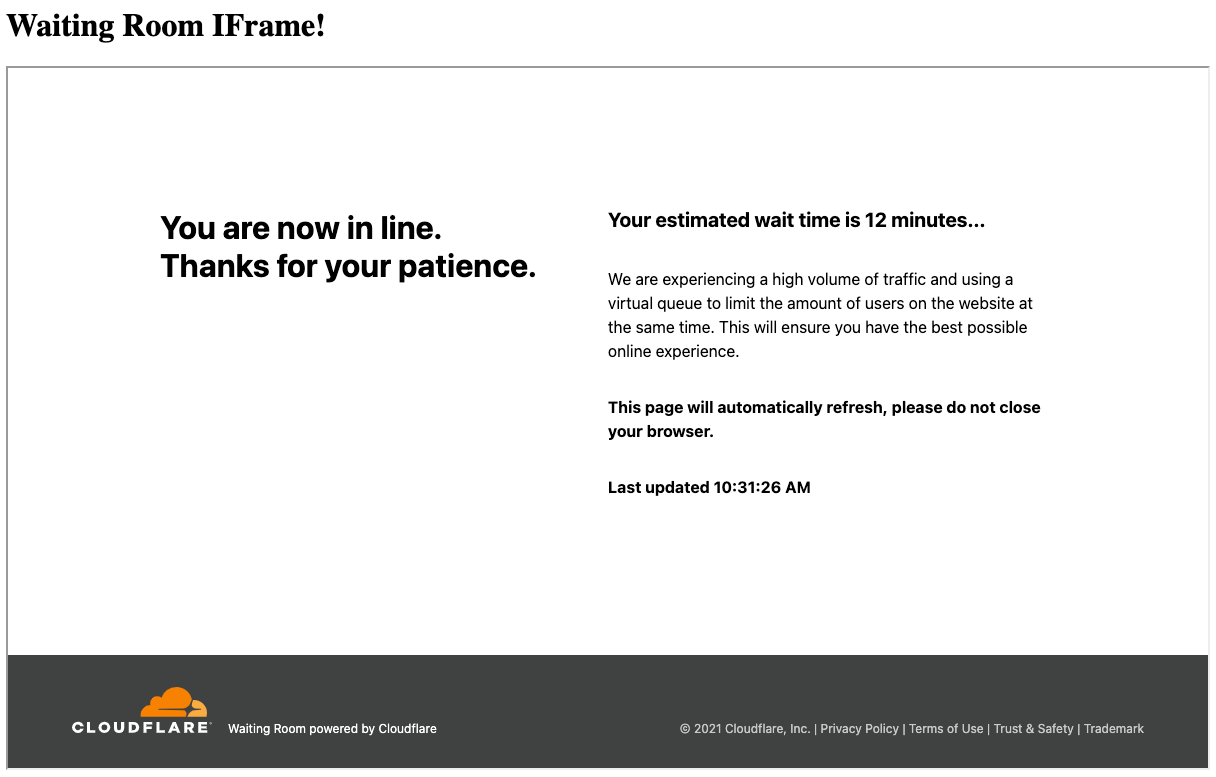
Why is this all important? In the past, we did not set SameSite, meaning it defaulted to SameSite=Lax for all responses. As a result, a user queueing through an IFrame would never have its cookie updated and appear to the Waiting Room as joining for the first time on every request. Today, we are introducing customization for both the SameSite and Secure attributes, which will allow Waiting Rooms to be displayed in IFrames!

At the moment, this is only configurable through the Cloudflare API. By default, the configuration for SameSite and Secure will be set to “auto”, automatically selecting the most flexible option. In this case, SameSite will be set to None if Always Use HTTPS is enabled, otherwise it will be set to Lax. Similarly, Secure will only be set if Always Use HTTPS is enabled. In other words, Waiting Room IFrames will work properly by default as long as Always Use HTTPS is toggled. If you are wondering why Always Use HTTPS is used here, remember that SameSite=None requires that Secure is also set, or else the browser will block the Waiting Room cookie.

If you decide to manually configure the behavior of SameSite and Secure through the API, be careful! We do guard against setting SameSite=None without Secure, but if you decide to set Secure on every request (secure=”always”) and don’t have Always Use HTTPS enabled, this means that a user who sends an insecure (HTTP) request to the Waiting Room will have its cookie blocked by its browser!

If you want to explore using IFrames with Waiting Room yourself, here is a simple example of a Cloudflare Worker that renders the Waiting Room on “https://example.com/waitingroom” in an IFrame:

const html = `<!DOCTYPE html>
<html>
 <head>
   <meta charset="UTF-8" />
   <meta name="viewport" content="width=device-width,initial-scale=1" />
   <title>Waiting Room IFrame Example</title>
 </head>
 <body>
   <h1>Waiting Room IFrame!</h1>
   <iframe src="https://example.com/waitingroom" width="1200" height="700"></iframe>
 </body>
</html>
`
 
addEventListener('fetch', event => {
 event.respondWith(handleRequest(event.request))
})
 
async function handleRequest(request) {
 return new Response(html, {
   headers: { "Content-Type": "text/html" },
 })
}
Waiting Room: Random Queueing and Custom Web/Mobile Apps

Looking Forward

Waiting Room still has plenty of room to grow! Every day, we are seeing more Waiting Rooms deployed to protect websites from traffic spikes. As Waiting Room continues to be used for new purposes, we will keep adding features to make it as customizable and user-friendly as possible.

Stay tuned — what we have announced today is just the tip of the iceberg of what we have planned for Waiting Room!
[$] A rough start for ksmbd

Post Syndicated from original https://lwn.net/Articles/871866/rss

Among the many new features pulled into the mainline during the 5.15 merge
window is the ksmbd
network filesystem server. Ksmbd implements the SMB protocol
(also known as CIFS, though that name has gone out of favor) that is
heavily used in the Windows world. The creation of an in-kernel SMB server
is a bit surprising, given that Linux has benefited greatly from the
user-space Samba solution since
shortly after the
beginning. There are reasons for this move but, in the short term at
least, they risk being overshadowed by a worrisome stream of
security-related problems in ksmbd.

Field Notes: How to Build an AWS Glue Workflow using the AWS Cloud Development Kit

Post Syndicated from Michael Hamilton original https://aws.amazon.com/blogs/architecture/field-notes-how-to-build-an-aws-glue-workflow-using-the-aws-cloud-development-kit/

Many customers use AWS Glue workflows to build and orchestrate their ETL (extract-transform-load) pipelines directly in the AWS Glue console using the visual tool to author workflows. This can be time consuming, harder to version control, and error prone due to manual configurations, when compared to managing your workflows as code. To improve your operational excellence, consider deploying the entire AWS Glue ETL pipeline using the AWS Cloud Development Kit (AWS CDK).

In this blog post, you will learn how to build an AWS Glue workflow using Amazon Simple Storage Service (Amazon S3), various components of AWS Glue, AWS Secrets Manager, Amazon Redshift, and the AWS CDK.

Architecture overview

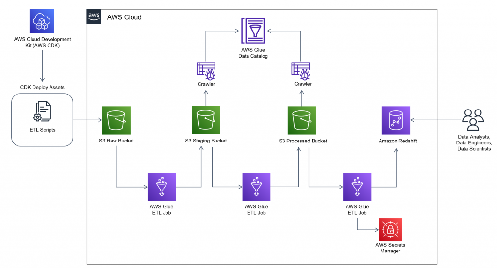
In this architecture, you will use the AWS CDK to deploy your data sources, ETL scripts, AWS Glue workflow components, and an Amazon Redshift cluster for analyzing the transformed data.

AWS Glue workflow architecture

Figure 1. AWS Glue workflow architecture

It is common for customers to pre-aggregate data before sending it downstream to analytical engines, like Amazon Redshift, because table joins and aggregations are computationally expensive. The AWS Glue workflow will join COVID-19 case data, and COVID-19 hiring data together on their date columns in order to run correlation analysis on the final dataset. The datasets may seem arbitrary, but we wanted to offer a way to better understand the impacts COVID-19 had on jobs in the United States. The takeaway here is to use this as a blueprint for automating the deployment of data analytic pipelines for the data of interest to your business.

After the AWS CDK application is deployed, it will begin creating all of the resources required to build the complete workflow. When it completes, the components in the architecture will be created, and the AWS Glue workflow will be ready to start. In this blog post, you start workflows manually, but they can be configured to start on a scheduled time or from a workflow trigger.

The workflow is programmed to dynamically pull the raw data from the Registry of Open Data on AWS where you can find the Covid-19 case data and the Hiring Data respectively.

Prerequisites

This blog post uses an AWS CDK stack written in TypeScript and AWS Glue jobs written in Python. Follow the instructions in the AWS CDK Getting Started guide to set up your environment, before you proceed to deployment.

In addition to setting up your environment, you need to clone the Git repository, which contains the AWS CDK scripts and Python ETL scripts used by AWS Glue. The ETL scripts will be deployed to Amazon S3 by the AWS CDK stack as assets, and referenced by the AWS Glue jobs as part of the AWS Glue Workflow.

You should have the following prerequisites:

Deployment

After you have cloned the repository, navigate to the glue-cdk-blog/lib folder and open the blog-glue-workflow-stack.ts file. This is the AWS CDK script used to deploy all necessary resources to build your AWS Glue workflow. The blog-redshift-vpc-stack.ts contains the necessary resources to deploy the Amazon Redshift cluster, connections, and permissions. The glue-cdk-blog/lib/assets folder also contains the AWS Glue job scripts. These files are uploaded to Amazon S3 by the AWS CDK when you bootstrap.

You won’t review the individual lines of code in the script in this blog post, but if you are unfamiliar with any of the AWS CDK level 1 or level 2 constructs used in the sample, you can review what each construct does with the AWS CDK documentation. Familiarize yourself with the script you cloned and anticipate what resources will be deployed. Then, deploy both stacks and verify your initial findings.

After your environment is configured, and the packages and modules installed, deploy the AWS CDK stack and assets in two commands.

  1. Bootstrap the AWS CDK stack to create an S3 bucket in the predefined account that will contain the assets.

cdk bootstrap

  1. Deploy the AWS CDK stacks.

cdk deploy --all

Verify that both of these commands have completed successfully, and remediate any failures returned. Upon successful completion, you’re ready to start the AWS Glue workflow that was just created. You can find the AWS CDK commands reference in the AWS CDK Toolkit commands documentation, and help with Troubleshooting common AWS CDK issues you may encounter.

Walkthrough

Prior to initiating the AWS Glue workflow, explore the resources the AWS CDK stacks just deployed to your account.

  1. Log in to the AWS Management Console and the AWS CDK account.
  2. Navigate to Amazon S3 in the AWS console (you should see an S3 bucket with the name prefix of cdktoolkit-stagingbucket-xxxxxxxxxxxx).
  3. Review the objects stored in the bucket in the assets folder. These are the .py files used by your AWS Glue jobs. They were uploaded to the bucket when you issued the AWS CDK bootstrap command, and referenced within the AWS CDK script as the scripts to use for the AWS Glue jobs. When retrieving data from multiple sources, you cannot always control the naming convention of the sourced files. To solve this and create better standardization, you will use a job within the AWS Glue workflow to copy these scripts to another folder and rename them with a more meaningful name.
  4. Navigate to Amazon Redshift in the AWS console and verify your new cluster. You can use the Amazon Redshift Query Editor within the console to connect to the cluster and see that you have an empty database called db-covid-hiring. The Amazon Redshift cluster and networking resources were created by the redshift_vpc_stack which are listed here:
    • VPC, subnet and security group for Amazon Redshift
    • Secrets Manager secret
    • AWS Glue connection and S3 endpoint
    • Amazon Redshift cluster
  1. Navigate to AWS Glue in the AWS console and review the following new resources created by the workflow_stack CDK stack:
    • Two crawlers to crawl the data in S3
    • Three AWS Glue jobs used within the AWS Glue workflow
    • Five triggers to initiate AWS Glue jobs and crawlers
    • One AWS Glue workflow to manage the ETL orchestration
  1. All of these resources could have been deployed within a single stack, but this is intended to be a simple example on how to share resources across multiple stacks. The AWS Identity and Access Management (IAM) role that AWS Glue uses to run the ETL jobs in the workflow_stack, is also used by Secrets Manager for Amazon Redshift in the redshift_vpc_stack. Inspect the /bin/blog-glue-workflow-stack.ts file to further understand cross stack resource sharing.

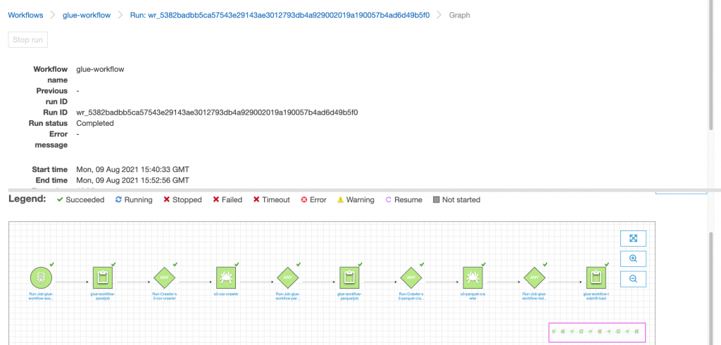
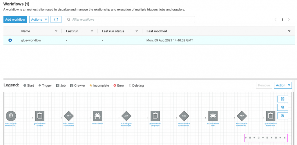
By performing these steps, you have deployed all of the AWS Glue resources necessary to perform common ETL tasks. You then combined the resources to create an orchestration of tasks using an AWS Glue workflow. All of this was done using IaC with AWS CDK. Your workflow should look like Figure 2.

AWS Glue console showing the workflow created by the CDK

Figure 2. AWS Glue console showing the workflow created by the CDK

As mentioned earlier, you could have started your workflow using a scheduled cron trigger, but you initiated the workflow manually so you had time to review the resources the workflow_stack CDK deployed, prior to initiation of the workflow. Now that you have reviewed the resources, validate your workflow by initiating it and verifying it runs successfully.

  1. From within the AWS Glue console, select Workflows under ETL.
  2. Select the workflow named glue-workflow, and then select Run from the actions listbox.
  3. You can verify the status of the workflow by viewing the run details under the History tab.
  4. Your job will take approximately 15 minutes to successfully complete, and your history should look like Figure 3.
AWS Glue console showing the workflow as completed after the run

Figure 3. AWS Glue console showing the workflow as completed after the run

The workflow performs the following tasks:

  1. Prepares the ETL scripts by copying the files in the S3 asset bucket to a new folder and renames them with a more relevant name.
  2. Initiates a crawler to crawl the raw source data as csv files and adds tables to the Glue Data Catalog.
  3. Runs a Python script to perform some ETL tasks on the .csv files and converts them to parquet files.
  4. Crawls the parquet files and adds them to the Glue Data Catalog.
  5. Loads the parquet files into a DynamicFrame and runs an Amazon Redshift COPY command to load the data into the Amazon Redshift database.

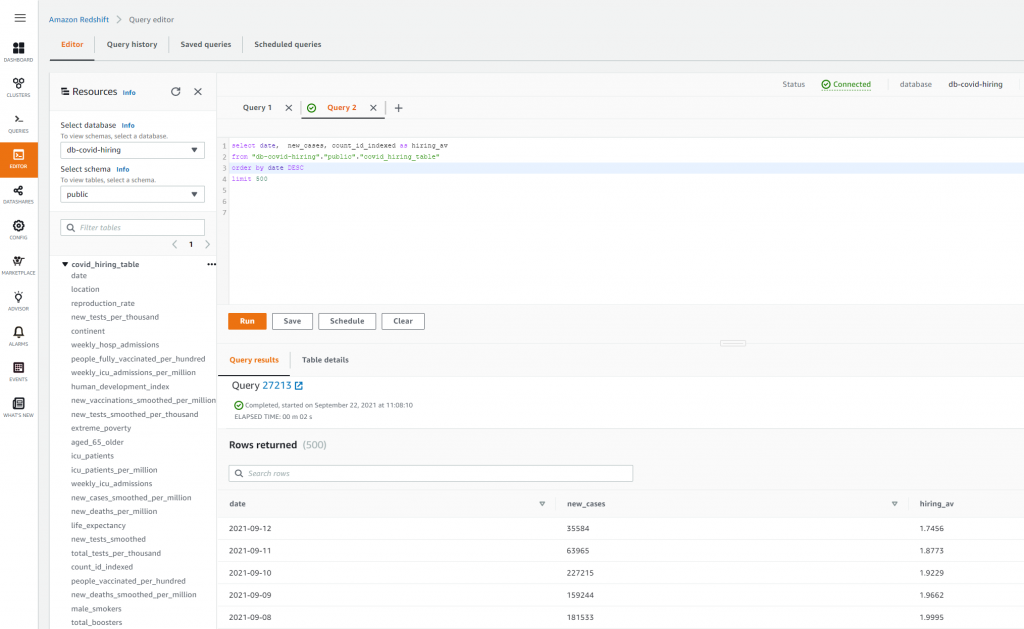
After the workflow completes, you can query and perform analytics on the data that was populated in Amazon Redshift. Open the Amazon Redshift Query Editor and run a simple SELECT statement to query the covid_hiring_table which is the joined Covid-19 case data and hiring data (see Figure 4).

Amazon Redshift query editor showing the data that the workflow loaded into the Redshift tables

Figure 4. Amazon Redshift query editor showing the data that the workflow loaded into the Redshift tables

Cleaning up

Some resources, like S3 buckets and Amazon DynamoDB tables, must be manually emptied and deleted through the console to be fully removed. To clean up the deployment, delete all objects in the AWS CDK asset bucket in Amazon S3 by using the AWS console to empty the bucket, and then run cdk destroy –all to delete the resources the AWS CDK stacks created in your account. Finally, if you don’t plan on using AWS CloudFormation assets in this account in the future, you will need to delete the AWS CDK asset stack within the CloudFormation console to remove the AWS CDK asset bucket.

Conclusion

In this blog post, you learned how to automate the deployment of AWS Glue workflows using the AWS CDK. This further enhances your continuous integration and delivery (CI/CD) data pipelines by automating the deployment of the ETL jobs and AWS Glue workflow orchestration, providing an efficient, fast, and repeatable way to build and deploy AWS Glue workflows at scale.

Although AWS CDK primarily supports level 1 constructs for most AWS Glue resources, new constructs are added continually. See the AWS CDK API Reference for updates, prior to authoring your stacks, for AWS Glue level 2 construct support. You can find the code used in this blog post in this GitHub repository, and the AWS CDK in TypeScript reference to the AWS CDK namespace.

We hope this blog post helps enrich your work through the skills gained of automating the creation of Glue Workflows, enabling you to quickly build and deploy your own ETL pipelines and run analytical models that power your business.

Field Notes provides hands-on technical guidance from AWS Solutions Architects, consultants, and technical account managers, based on their experiences in the field solving real-world business problems for customers.

Security updates for Thursday

Post Syndicated from original https://lwn.net/Articles/872154/rss

Security updates have been issued by Debian (firefox-esr), Mageia (cockpit, fail2ban, libcryptopp, libss7, nodejs, opendmarc, and weechat), openSUSE (curl, ffmpeg, git, glibc, go1.16, libcryptopp, and nodejs8), SUSE (apache2, curl, ffmpeg, git, glibc, go1.16, grilo, libcryptopp, nodejs8, transfig, and webkit2gtk3), and Ubuntu (linux-oem-5.10 and python-bottle).

Velociraptor to Announce Winners of Its 2021 Contributor Competition

Post Syndicated from Carlos Canto original https://blog.rapid7.com/2021/10/07/velociraptor-to-announce-winners-of-its-2021-contributor-competition/

Velociraptor to Announce Winners of Its 2021 Contributor Competition

Velociraptor and Rapid7 are excited to announce the winners of our 2021 Velociraptor Contributor Competition on Friday, October 8. This competition encourages development of useful content and extensions to the Velociraptor platform. Submissions include new functionality in the form of VQL artifacts, Velociraptor plugins, or new Velociraptor code and integrations. Judging will be done by a panel of various digital forensics and incident response (DFIR) industry leaders and security experts.

You can watch the announcement of the winners LIVE at the SANS Threat Hunting Summit on Friday, October 8th at 1 pm ET. To register for the summit, head to this page and click on the “Register for Summit” link. Registration is completely free.

Velociraptor to Announce Winners of Its 2021 Contributor Competition

The competition carries 3 prize levels: First prize is $5,000 USD, second prize is $3,000 USD, and third prize is $2,000 USD. The winning submissions will also be published on the Velociraptor website.

Velociraptor is an advanced DFIR tool that enhances visibility into all of your endpoints. To learn more about Velociraptor, visit our website or follow us on Twitter @velocidex.

Perspectives on supporting young people in low-income areas to access and engage with computing

Post Syndicated from Hayley Leonard original https://www.raspberrypi.org/blog/young-people-low-income-areas-computing-uk-usa-guyana/

The Raspberry Pi Foundation’s mission is to make computing and digital making accessible to all. To support young people at risk of educational disadvantage because they don’t have access to computing devices outside of school, we’ve set up the Learn at Home campaign. But access is only one part of the story. To learn more about what support these young people need across organisations and countries, we set up a panel discussion at the Tapia Celebration of Diversity in Computing conference.

Two young African women work at desktop computers.

The three panelists provided a stimulating discussion of some key issues in supporting young people in low-income areas in the UK, USA, and Guyana to engage with computing, and we hope their insights are of use to educators, youth workers, and organisations around the world.

The panellists and their perspectives

Our panellists represent three different countries, and all have experience of teaching in schools and/or working with young people outside of the formal education system. Because of the differences between countries in terms of access to computing, having this spread of expertise and contexts allowed the panelists to compare lessons learned in different sectors and locations.

Lenlandlar Singh

Panelist Lenandlar Singh is a Senior Lecturer in the Department of Computer Science at the University of Guyana. In Guyana, there is a range of computing-related courses for high school students, and access to optional qualifications in computer science at A level (age 17–18).

Yolanda Payne.

Panelist Yolanda Payne is a Research Associate at the Constellations Center at Georgia Tech, USA. In the US, computing curricula differ across states, although there is some national leadership through associations, centres, and corporations.

Christina Watson.

Christina Watson is Assistant Director of Design at UK Youth*, UK. The UK has a mandatory computing curriculum for learners aged 5–18, although curricula vary across the four home nations (England, Scotland, Wales, Northern Ireland).

As the moderator, I posed the following three questions, which the panelists answered from their own perspectives and experiences:

  • What are the key challenges for young people to engage with computing in or out of school, and what have you done to overcome these challenges?
  • What do you see as the role of formal and non-formal learning opportunities in computing for these young people?
  • What have you learned that could help other people working with these young people and their communities in the future?

Similarities across contexts

One of the aspects of the discussion that really stood out was the number of similarities across the panellists’ different contexts. 

The first of these similarities was the lack of access to computing amongst young people from low-income families, particularly in more rural areas, across all three countries. These access issues concerned devices and digital infrastructure, but also the types of opportunities in and out of school that young people were able to engage with.

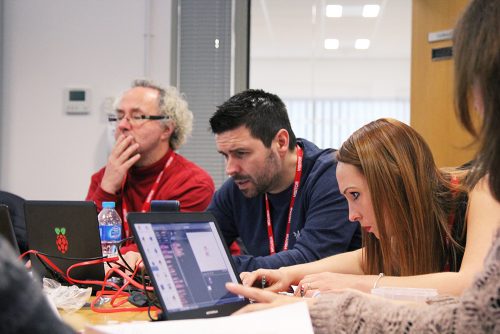
Two girls code at a desktop computer while a female mentor observes them.

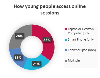
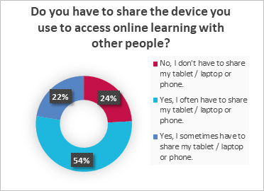
Christina (UK) shared results from a survey conducted with Aik Saath, a youth organisation in the UK Youth network (see graphs below). The results highlighted that very few young people in low-income areas had access to their own device for online learning, and mostly their access was to a smartphone or tablet rather than a computer. She pointed out that youth organisations can struggle to provide access to computing not only due to lack of funding, but also because they don’t have secure spaces in which to store equipment.

Lenandlar (Guyana) and Christina (UK) also discussed the need to improve the digital skills and confidence of teachers and youth workers so they can support young people with their computing education. While Lenandlar spoke about recruitment and training of qualified computing teachers in Guyana, Christina suggested that it was less important for youth workers in the UK to become experts in the field and more important for them to feel empowered and confident in supporting young people to explore computing and understand different career paths. UK Youth found that partnering with organisations that provided technical expertise (such as us at the Raspberry Pi Foundation) allowed youth workers to focus on the broader support that the young people needed.

Both Yolanda (US) and Lenandlar (Guyana) discussed the restrictive nature of the computing curriculum in schools, agreeing with Christina (UK) that outside of the classroom, there was more freedom for young people to explore different aspects of computing. All three agreed that introducing more fun and relevant activities into the curriculum made young people excited about computing and reduced stereotypes and misconceptions about the discipline and career. Yolanda explained that using modern, real-life examples and role models was a key part of connecting with young people and engaging them in computing.

What can teachers do to support young people and their families?

Yolanda (US) advocated strongly for listening to students and their communities to help understand what is meaningful and relevant to them. One example of this approach is to help young people and their families understand the economics of technology, and how computing can be used to support, develop, and sustain businesses and employment in their community. As society has become more reliant on computing and technology, this can translate into real economic impact.

A CoderDojo coding session for young people.

Both Yolanda (US) and Lenandlar (Guyana) emphasised the importance of providing opportunities for digital making, allowing students opportunities to become creators rather than just consumers of technology. They also highly recommended providing relevant contexts for computing and identifying links with different careers.

The panellists also discussed the importance of partnering with other education settings, with tech companies, and with non-profit organisations to provide access to equipment and opportunities for students in schools that have limited budgets and capacity for computing. These links can also highlight key role models and help to build strong relationships in the community between businesses and schools.

What is the role of non-formal settings in low-income areas?

All of the panellists agreed that non-formal settings provided opportunities for further exploration and skill development outside of a strict curriculum. Christina (UK) particularly highlighted that these settings helped support young people and families who feel left behind by the education system, allowing them to develop practical skills and knowledge that can help their whole family. She emphasised the strong relationships that can be developed in these settings and how these can provide relatable role models for young people in low-income areas.

A young girl uses a computer.

Tips and suggestions

After the presentation, the panelists responded to the audience’s questions with some practical tips and suggestions for engaging young people in low-income communities with computing:

How do you engage young people who are non-native English speakers with mainly English computing materials?

  • For curriculum materials, it’s possible to use Google Translate to allow students to access them. The software is not always totally accurate but goes some way to supporting these students. You can also try to use videos that have captioning and options for non-English subtitles.
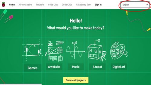
  • We offer translated versions of our free online projects, thanks to a community of dedicated volunteer translators from around the world. Learners can choose from up to 30 languages (as shown in the picture below).
The Raspberry Pi Foundation's projects website, with the drop-down menu to choose a human language highlighted.
Young people can learn about computing in their first language by using the menu on our projects site.

How do you set up partnerships with other organisations?

  • Follow companies on social media and share how you are using their products or tools, and how you are aligned with their goals. This can form the basis of future partnerships.
  • When you are actively applying for partnerships, consider the following points:
    • What evidence do you have that you need support from the potential partner?
    • What support are you asking for? This may differ across potential partners, so make sure your pitch is relevant and tailored to a specific partner.
    • What evidence could you use to show the impact you are already having or previous successful projects or partnerships?

Make use of our free training resources and guides

For anyone wishing to learn computing knowledge and skills, and the skills you need to teach young people in and out of school about these topics, we provide a wide range of free online training courses to cover all your needs. Educators in England can also access the free CPD that we and our consortium partners offer through the National Centre for Computing Education.

To help you support your learners in and out of school to engage with computing in ways that are meaningful and relevant for them, we recently published a guide on culturally relevant teaching.

We also support a worldwide network of volunteers to run CoderDojos, which are coding clubs for young people in local community spaces. Head over to the CoderDojo website to discover more about the free materials and help we’ve got for you.

We would like to thank our panellists Lenandlar Singh, Yolanda Payne, and Christina Watson for sharing their time and expertise, and the Tapia conference organisers for providing a great platform to discuss issues of diversity, equality, and inclusion in computing.


*UK Youth is a leading charity working across the UK with an open network of over 8000 youth organisations. The charity has influence as a sector-supporting infrastructure body, a direct delivery partner, and a campaigner for social change.

The post Perspectives on supporting young people in low-income areas to access and engage with computing appeared first on Raspberry Pi.

Simulated location data with Amazon Location Service

Post Syndicated from Aaron Sempf original https://aws.amazon.com/blogs/devops/simulated-location-data-with-amazon-location-service/

Modern location-based applications require the processing and storage of real-world assets in real-time. The recent release of Amazon Location Service and its Tracker feature makes it possible to quickly and easily build these applications on the AWS platform. Tracking real-world assets is important, but at some point when working with Location Services you will need to demo or test location-based applications without real-world assets.

Applications that track real-world assets are difficult to test and demo in a realistic setting, and it can be hard to get your hands on large amounts of real-world location data. Furthermore, not every company or individual in the early stages of developing a tracking application has access to a large fleet of test vehicles from which to derive this data.

Location data can also be considered highly sensitive, because it can be easily de-anonymized to identify individuals and movement patterns. Therefore, only a few openly accessible datasets exist and are unlikely to exhibit the characteristics required for your particular use-case.

To overcome this problem, the location-based services community has developed multiple openly available location data simulators. This blog will demonstrate how to connect one of those simulators to Amazon Location Service Tracker to test and demo your location-based services on AWS.

Walk-through

Part 1: Create a tracker in Amazon Location Service

This walkthrough will demonstrate how to get started setting up simulated data into your tracker.

Amazon location Service console
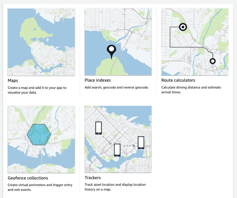
Step 1: Navigate to Amazon Location Service in the AWS Console and select “Trackers“.

Step 2: On the “Trackers” screen click the orange “Create tracker“ button.

Select Create Tracker

Create a Tracker form

Step 3: On the “Create tracker” screen, name your tracker and make sure to reply “Yes” to the question asking you if you will only use simulated or sample data. This allows you to use the free-tier of the service.

Next, click “Create tracker” to create you tracker.

Confirm create tracker

Done. You’ve created a tracker. Note the “Name” of your tracker.

Generate trips with the SharedStreets Trip-simulator

A common option for simulating trip data is the shared-steets/trip-simulator project.

SharedStreets maintains an open-source project on GitHub – it is a probabilistic, multi-agent GPS trajectory simulator. It even creates realistic noise, and thus can be used for testing algorithms that must work under real-world conditions. Of course, the generated data is fake, so privacy is not a concern.

The trip-simulator generates files with a single GPS measurement per line. To playback those files to the Amazon Location Service Tracker, you must use a tool to parse the file; extract the GPS measurements, time measurements, and device IDs of the simulated vehicles; and send them to the tracker at the right time.

Before you start working with the playback program, the trip-simulator requires a map to simulate realistic trips. Therefore, you must download a part of OpenStreetMap (OSM). Using GeoFabrik you can download extracts at the size of states or selected cities based on the area within which you want to simulate your data.

This blog will demonstrate how to simulate a small fleet of cars in the greater Munich area. The example will be written for OS-X, but it generalizes to Linux operating systems. If you have a Windows operating system, I recommend using Windows Subsystem for Linux (WSL). Alternatively, you can run this from a Cloud9 IDE in your AWS account.

Step 1: Download the Oberbayern region from download.geofabrik.de

Prerequisites:

curl https://download.geofabrik.de/europe/germany/bayern/oberbayern-latest.osm.pbf -o oberbayern-latest.osm.pbf

Step 2: Install osmium-tool

Prerequisites:

brew install osmium-tool

Step 3: Extract Munich from the Oberbayern map

osmium extract -b "11.5137,48.1830,11.6489,48.0891" oberbayern-latest.osm.pbf -o ./munich.osm.pbf -s "complete_ways" --overwrite

Step 4: Pre-process the OSM map for the vehicle routing

Prerequisites:

docker run -t -v $(pwd):/data osrm/osrm-backend:v5.25.0 osrm-extract -p /opt/car.lua /data/munich.osm.pbf
docker run -t -v $(pwd):/data osrm/osrm-backend:v5.25.0 osrm-contract /data/munich.osrm

Step 5: Install the trip-simulator

Prerequisites:

npm install -g trip-simulator

Step 6: Run a 10 car, 30 minute car simulation

trip-simulator \
  --config car \
  --pbf munich.osm.pbf \
  --graph munich.osrm \
  --agents 10 \
  --start 1563122921000 \
  --seconds 1800 \
  --traces ./traces.json \
  --probes ./probes.json \
  --changes ./changes.json \
  --trips ./trips.json

The probes.json file is the file containing the GPS probes we will playback to Amazon Location Service.

Part 2: Playback trips to Amazon Location Service

Now that you have simulated trips in the probes.json file, you can play them back in the tracker created earlier. For this, you must write only a few lines of Python code. The following steps have been neatly separated into a series of functions that yield an iterator.

Prerequisites:

Step 1: Load the probes.json file and yield each line

import json
import time
import datetime
import boto3

def iter_probes_file(probes_file_name="probes.json"):
    """Iterates a file line by line and yields each individual line."""
    with open(probes_file_name) as probes_file:
        while True:
            line = probes_file.readline()
            if not line:
                break
            yield line

Step 2: Parse the probe on each line
To process the probes, you parse the JSON on each line and extract the data relevant for the playback. Note that the coordinates order is longitude, latitude in the probes.json file. This is the same order that the Location Service expects.

def parse_probes_trip_simulator(probes_iter):
    """Parses a file witch contains JSON document, one per line.
    Each line contains exactly one GPS probe. Example:
    {"properties":{"id":"RQQ-7869","time":1563123002000,"status":"idling"},"geometry":{"type":"Point","coordinates":[-86.73903753135207,36.20418779626351]}}
    The function returns the tuple (id,time,status,coordinates=(lon,lat))
    """
    for line in probes_iter:
        probe = json.loads(line)
        props = probe["properties"]
        geometry = probe["geometry"]
        yield props["id"], props["time"], props["status"], geometry["coordinates"]

Step 3: Update probe record time

The probes represent historical data. Therefore, when you playback you will need to normalize the probes recorded time to sync with the time you send the request in order to achieve the effect of vehicles moving in real-time.

This example is a single threaded playback. If the simulated playback lags behind the probe data timing, then you will be provided a warning through the code detecting the lag and outputting a warning.

The SharedStreets trip-simulator generates one probe per second. This frequency is too high for most applications, and in real-world applications you will often see frequencies of 15 to 60 seconds or even less. You must decide if you want to add another iterator for sub-sampling the data.

def update_probe_record_time(probes_iter):
    """
    Modify all timestamps to be relative to the time this function was called.
    I.e. all timestamps will be equally spaced from each other but in the future.
    """
    new_simulation_start_time_utc_ms = datetime.datetime.now().timestamp() * 1000
    simulation_start_time_ms = None
    time_delta_recording_ms = None
    for i, (_id, time_ms, status, coordinates) in enumerate(probes_iter):
        if time_delta_recording_ms is None:
            time_delta_recording_ms = new_simulation_start_time_utc_ms - time_ms
            simulation_start_time_ms = time_ms
        simulation_lag_sec = (
            (
                datetime.datetime.now().timestamp() * 1000
                - new_simulation_start_time_utc_ms
            )
            - (simulation_start_time_ms - time_ms)
        ) / 1000
        if simulation_lag_sec > 2.0 and i % 10 == 0:
            print(f"Playback lags behind by {simulation_lag_sec} seconds.")
        time_ms += time_delta_recording_ms
        yield _id, time_ms, status, coordinates

Step 4: Playback probes
In this step, pack the probes into small batches and introduce the timing element into the simulation playback. The reason for placing them in batches is explained below in step 6.

def sleep(time_elapsed_in_batch_sec, last_sleep_time_sec):
    sleep_time = max(
        0.0,
        time_elapsed_in_batch_sec
        - (datetime.datetime.now().timestamp() - last_sleep_time_sec),
    )
    time.sleep(sleep_time)
    if sleep_time > 0.0:
        last_sleep_time_sec = datetime.datetime.now().timestamp()
    return last_sleep_time_sec


def playback_probes(
    probes_iter,
    batch_size=10,
    batch_window_size_sec=2.0,
):
    """
    Replays the probes in live mode.
    The function assumes, that the probes returned by probes_iter are sorted
    in ascending order with respect to the probe timestamp.
    It will either yield batches of size 10 or smaller batches if the timeout is reached.
    """
    last_probe_record_time_sec = None
    time_elapsed_in_batch_sec = 0
    last_sleep_time_sec = datetime.datetime.now().timestamp()
    batch = []
    # Creates two second windows and puts all the probes falling into
    # those windows into a batch. If the max. batch size is reached it will yield early.
    for _id, time_ms, status, coordinates in probes_iter:
        probe_record_time_sec = time_ms / 1000
        if last_probe_record_time_sec is None:
            last_probe_record_time_sec = probe_record_time_sec
        time_to_next_probe_sec = probe_record_time_sec - last_probe_record_time_sec
        if (time_elapsed_in_batch_sec + time_to_next_probe_sec) > batch_window_size_sec:
            last_sleep_time_sec = sleep(time_elapsed_in_batch_sec, last_sleep_time_sec)
            yield batch
            batch = []
            time_elapsed_in_batch_sec = 0
        time_elapsed_in_batch_sec += time_to_next_probe_sec
        batch.append((_id, time_ms, status, coordinates))
        if len(batch) == batch_size:
            last_sleep_time_sec = sleep(time_elapsed_in_batch_sec, last_sleep_time_sec)
            yield batch
            batch = []
            time_elapsed_in_batch_sec = 0
        last_probe_record_time_sec = probe_record_time_sec
    if len(batch) > 0:
        last_sleep_time_sec = sleep(time_elapsed_in_batch_sec, last_sleep_time_sec)
        yield batch

Step 5: Create the updates for the tracker

LOCAL_TIMEZONE = (
    datetime.datetime.now(datetime.timezone(datetime.timedelta(0))).astimezone().tzinfo
)

def convert_to_tracker_updates(probes_batch_iter):
    """
    Converts batches of probes in the format (id,time_ms,state,coordinates=(lon,lat))
    into batches ready for upload to the tracker.
    """
    for batch in probes_batch_iter:
        updates = []
        for _id, time_ms, _, coordinates in batch:
            # The boto3 location service client expects a datetime object for sample time
            dt = datetime.datetime.fromtimestamp(time_ms / 1000, LOCAL_TIMEZONE)
            updates.append({"DeviceId": _id, "Position": coordinates, "SampleTime": dt})
        yield updates

Step 6: Send the updates to the tracker
In the update_tracker function, you use the batch_update_device_position function of the Amazon Location Service Tracker API. This lets you send batches of up to 10 location updates to the tracker in one request. Batching updates is much more cost-effective than sending one-by-one. You pay for each call to batch_update_device_position. Therefore, batching can lead to a 10x cost reduction.

def update_tracker(batch_iter, location_client, tracker_name):
    """
    Reads tracker updates from an iterator and uploads them to the tracker.
    """
    for update in batch_iter:
        response = location_client.batch_update_device_position(
            TrackerName=tracker_name, Updates=update
        )
        if "Errors" in response and response["Errors"]:
            for error in response["Errors"]:
                print(error["Error"]["Message"])

Step 7: Putting it all together
The follow code is the main section that glues every part together. When using this, make sure to replace the variables probes_file_name and tracker_name with the actual probes file location and the name of the tracker created earlier.

if __name__ == "__main__":
    location_client = boto3.client("location")
    probes_file_name = "probes.json"
    tracker_name = "my-tracker"
    iterator = iter_probes_file(probes_file_name)
    iterator = parse_probes_trip_simulator(iterator)
    iterator = update_probe_record_time(iterator)
    iterator = playback_probes(iterator)
    iterator = convert_to_tracker_updates(iterator)
    update_tracker(
        iterator, location_client=location_client, tracker_name=tracker_name
    )

Paste all of the code listed in steps 1 to 7 into a file called trip_playback.py, then execute

python3 trip_playback.py

This will start the playback process.

Step 8: (Optional) Tracking a device’s position updates
Once the playback is running, verify that the updates are actually written to the tracker repeatedly querying the tracker for updates for a single device. Here, you will use the get_device_position function of the Amazon Location Service Tracker API to receive the last known device position.

import boto3
import time

def get_last_vehicle_position_from_tracker(
    device_id, tracker_name="your-tracker", client=boto3.client("location")
):
    response = client.get_device_position(DeviceId=device_id, TrackerName=tracker_name)
    if response["ResponseMetadata"]["HTTPStatusCode"] != 200:
        print(str(response))
    else:
        lon = response["Position"][0]
        lat = response["Position"][1]
        return lon, lat, response["SampleTime"]
        
if __name__ == "__main__":   
    device_id = "my-device"     
    tracker_name = "my-tracker"
    while True:
        lon, lat, sample_time = get_last_vehicle_position_from_tracker(
            device_id=device_id, tracker_name=tracker_name
        )
        print(f"{lon}, {lat}, {sample_time}")
        time.sleep(10)

In the example above, you must replace the tracker_name with the name of the tracker created earlier and the device_id with the ID of one of the simulation vehicles. You can find the vehicle IDs in the probes.json file created by the SharedStreets trip-simulator. If you run the above code, then you should see the following output.

location probes data

AWS IoT Device Simulator

As an alternative, if you are familiar with AWS IoT, AWS has its own vehicle simulator that is part of the IoT Device Simulator solution. It lets you simulate a vehicle fleet moving on a road network. This has been described here. The simulator sends the location data to an Amazon IoT endpoint. The Amazon Location Service Developer Guide shows how to write and set-up a Lambda function to connect the IoT topic to the tracker.

The AWS IoT Device Simulator has a GUI and is a good choice for simulating a small number of vehicles. The drawback is that only a few trips are pre-packaged with the simulator and changing them is somewhat complicated. The SharedStreets Trip-simulator has much more flexibility, allowing simulations of fleets made up of a larger number of vehicles, but it has no GUI for controlling the playback or simulation.

Cleanup

You’ve created a Location Service Tracker resource. It does not incur any charges if it isn’t used. If you want to delete it, you can do so on the Amazon Location Service Tracker console.

Conclusion

This blog showed you how to use an open-source project and open-source data to generate simulated trips, as well as how to play those trips back to the Amazon Location Service Tracker. Furthermore, you have access to the AWS IoT Device Simulator, which can also be used for simulating vehicles.

Give it a try and tell us how you test your location-based applications in the comments.

About the authors

Florian Seidel

Florian is a Solutions Architect in the EMEA Automotive Team at AWS. He has worked on location based services in the automotive industry for the last three years and has many years of experience in software engineering and software architecture.

Aaron Sempf

Aaron is a Senior Partner Solutions Architect, in the Global Systems Integrators team. When not working with AWS GSI partners, he can be found coding prototypes for autonomous robots, IoT devices, and distributed solutions.

Building an InnerSource ecosystem using AWS DevOps tools

Post Syndicated from Debashish Chakrabarty original https://aws.amazon.com/blogs/devops/building-an-innersource-ecosystem-using-aws-devops-tools/

InnerSource is the term for the emerging practice of organizations adopting the open source methodology, albeit to develop proprietary software. This blog discusses the building of a model InnerSource ecosystem that leverages multiple AWS services, such as CodeBuild, CodeCommit, CodePipeline, CodeArtifact, and CodeGuru, along with other AWS services and open source tools.

What is InnerSource and why is it gaining traction?

Most software companies leverage open source software (OSS) in their products, as it is a great mechanism for standardizing software and bringing in cost effectiveness via the re-use of high quality, time-tested code. Some organizations may allow its use as-is, while others may utilize a vetting mechanism to ensure that the OSS adheres to the organization standards of security, quality, etc. This confidence in OSS stems from how these community projects are managed and sustained, as well as the culture of openness, collaboration, and creativity that they nurture.

Many organizations building closed source software are now trying to imitate these development principles and practices. This approach, which has been perhaps more discussed than adopted, is popularly called “InnerSource”. InnerSource serves as a great tool for collaborative software development within the organization perimeter, while keeping its concerns for IP & Legality in check. It provides collaboration and innovation avenues beyond the confines of organizational silos through knowledge and talent sharing. Organizations reap the benefits of better code quality and faster time-to-market, yet at only a fraction of the cost.

What constitutes an InnerSource ecosystem?

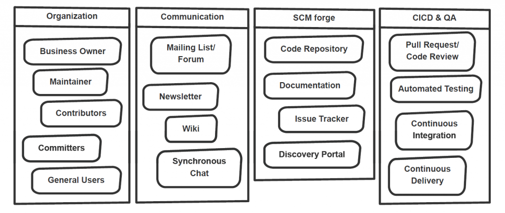
Infrastructure and processes that harbor collaboration stand at the heart of InnerSource ecology. These systems (refer Figure 1) would typically include tools supporting features such as code hosting, peer reviews, Pull Request (PR) approval flow, issue tracking, documentation, communication & collaboration, continuous integration, and automated testing, among others. Another major component of this system is an entry portal that enables the employees to discover the InnerSource projects and join the community, beginning as ordinary users of the reusable code and later graduating to contributors and committers.

A typical InnerSource ecosystem

Figure 1: A typical InnerSource ecosystem

More to InnerSource than meets the eye

This blog focuses on detailing a technical solution for establishing the required tools for an InnerSource system primarily to enable a development workflow and infrastructure. But the secret sauce of an InnerSource initiative in an enterprise necessitates many other ingredients.

InnerSource Roles & Use Cases

Figure 2: InnerSource Roles & Use Cases

InnerSource thrives on community collaboration and a low entry barrier to enable adoptability. In turn, that demands a cultural makeover. While strategically deciding on the projects that can be inner sourced as well as the appropriate licensing model, enterprises should bootstrap the initiative with a seed product that draws the community, with maintainers and the first set of contributors. Many of these users would eventually be promoted, through a meritocracy-based system, to become the trusted committers.

Over a set period, the organization should plan to move from an infra specific model to a project specific model. In a Project-specific InnerSource model, the responsibility for a particular software asset is owned by a dedicated team funded by other business units. Whereas in the Infrastructure-based InnerSource model, the organization provides the necessary infrastructure to create the ecosystem with code & document repositories, communication tools, etc. This enables anybody in the organization to create a new InnerSource project, although each project initiator maintains their own projects. They could begin by establishing a community of practice, and designating a core team that would provide continuing support to the InnerSource projects’ internal customers. Having a team of dedicated resources would clearly indicate the organization’s long-term commitment to sustaining the initiative. The organization should promote this culture through regular boot camps, trainings, and a recognition program.

Lastly, the significance of having a modular architecture in the InnerSource projects cannot be understated. This architecture helps developers understand the code better, as well as aids code reuse and parallel development, where multiple contributors could work on different code modules while avoiding conflicts during code merges.

A model InnerSource solution using AWS services

This blog discusses a solution that weaves various services together to create the necessary infrastructure for an InnerSource system. While it is not a full-blown solution, and it may lack some other components that an organization may desire in its own system, it can provide you with a good head start.

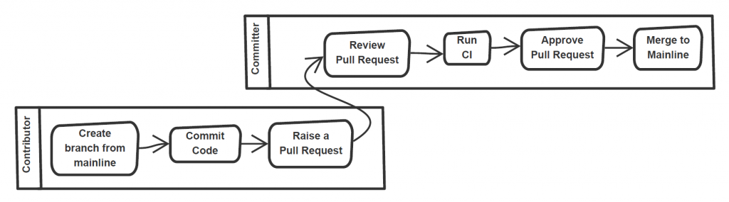
The ultimate goal of the model solution is to enable a developer workflow as depicted in Figure 3.

Typical developer workflow at InnerSource

Figure 3: Typical developer workflow at InnerSource

At the core of the InnerSource-verse is the distributed version control (AWS CodeCommit in our case). To maintain system transparency, openness, and participation, we must have a discovery mechanism where users could search for the projects and receive encouragement to contribute to the one they prefer (Step 1 in Figure 4).

Architecture diagram for the model InnerSource system

Figure 4: Architecture diagram for the model InnerSource system

For this purpose, the model solution utilizes an open source reference implantation of InnerSource Portal. The portal indexes data from AWS CodeCommit by using a crawler, and it lists available projects with associated metadata, such as the skills required, number of active branches, and average number of commits. For CodeCommit, you can use the crawler implementation that we created in the open source code repo at https://github.com/aws-samples/codecommit-crawler-innersource.

The major portal feature is providing an option to contribute to a project by using a “Contribute” link. This can present a pop-up form to “apply as a contributor” (Step 2 in Figure 4), which when submitted sends an email (or creates a ticket) to the project maintainer/committer who can create an IAM (Step 3 in Figure 4) user with access to the particular repository. Note that the pop-up form functionality is built into the open source version of the portal. However, it would be trivial to add one with an associated action (send an email, cut a ticket, etc.).

InnerSource portal indexes CodeCommit repos and provides a bird’s eye view

Figure 5: InnerSource portal indexes CodeCommit repos and provides a bird’s eye view

The contributor, upon receiving access, logs in to CodeCommit, clones the mainline branch of the InnerSource project (Step 4 in Figure 4) into a fix or feature branch, and starts altering/adding the code. Once completed, the contributor commits the code to the branch and raises a PR (Step 5 in Figure 4). A Pull Request is a mechanism to offer code to an existing repository, which is then peer-reviewed and tested before acceptance for inclusion.

The PR triggers a CodeGuru review (Step 6 in Figure 4) that adds the recommendations as comments on the PR. Furthermore, it triggers a CodeBuild process (Steps 7 to 10 in Figure 4) and logs the build result in the PR. At this point, the code can be peer reviewed by Trusted Committers or Owners of the project repository. The number of approvals would depend on the approval template rule configured in CodeCommit. The Committer(s) can approve the PR (Step 12 in Figure 4) and merge the code to the mainline branch – that is once they verify that the code serves its purpose, has passed the required tests, and doesn’t break the build. They could also rely on the approval vote from a sanity test conducted by a CodeBuild process. Optionally, a build process could deploy the latest mainline code (Step 14 in Figure 4) on the PR merge commit.

To maintain transparency in all communications related to progress, bugs, and feature requests to downstream users and contributors, a communication tool may be needed. This solution does not show integration with any Issue/Bug tracking tool out of the box. However, multiple of these tools are available at the AWS marketplace, with some offering forum and Wiki add-ons in order to elicit discussions. Standard project documentation can be kept within the repository by using the constructs of the README.md file to provide project mission details and the CONTRIBUTING.md file to guide the potential code contributors.

An overview of the AWS services used in the model solution

The model solution employs the following AWS services:

  • Amazon CodeCommit: a fully managed source control service to host secure and highly scalable private Git repositories.
  • Amazon CodeBuild: a fully managed build service that compiles source code, runs tests, and produces software packages that are ready to deploy.
  • Amazon CodeDeploy: a service that automates code deployments to any instance, including EC2 instances and instances running on-premises.
  • Amazon CodeGuru: a developer tool providing intelligent recommendations to improve code quality and identify an application’s most expensive lines of code.
  • Amazon CodePipeline: a fully managed continuous delivery service that helps automate release pipelines for fast and reliable application and infrastructure updates.
  • Amazon CodeArtifact: a fully managed artifact repository service that makes it easy to securely store, publish, and share software packages utilized in their software development process.
  • Amazon S3: an object storage service that offers industry-leading scalability, data availability, security, and performance.
  • Amazon EC2: a web service providing secure, resizable compute capacity in the cloud. It is designed to ease web-scale computing for developers.
  • Amazon EventBridge: a serverless event bus that eases the building of event-driven applications at scale by using events generated from applications and AWS services.
  • Amazon Lambda: a serverless compute service that lets you run code without provisioning or managing servers.

The journey of a thousand miles begins with a single step

InnerSource might not be the right fit for every organization, but is a great step for those wanting to encourage a culture of quality and innovation, as well as purge silos through enhanced collaboration. It requires backing from leadership to sponsor the engineering initiatives, as well as champion the establishment of an open and transparent culture granting autonomy to the developers across the org to contribute to projects outside of their teams. The organizations best-suited for InnerSource have already participated in open source initiatives, have engineering teams that are adept with CI/CD tools, and are willing to adopt OSS practices. They should start small with a pilot and build upon their successes.

Conclusion

Ever more enterprises are adopting the open source culture to develop proprietary software by establishing an InnerSource. This instills innovation, transparency, and collaboration that result in cost effective and quality software development. This blog discussed a model solution to build the developer workflow inside an InnerSource ecosystem, from project discovery to PR approval and deployment. Additional features, like an integrated Issue Tracker, Real time chat, and Wiki/Forum, can further enrich this solution.

If you need helping hands, AWS Professional Services can help adapt and implement this model InnerSource solution in your enterprise. Moreover, our Advisory services can help establish the governance model to accelerate OSS culture adoption through Experience Based Acceleration (EBA) parties.

References

About the authors

Debashish Chakrabarty

Debashish Chakrabarty

Debashish is a Senior Engagement Manager at AWS Professional Services, India managing complex projects on DevOps, Security and Modernization and help ProServe customers accelerate their adoption of AWS Services. He loves to keep connected to his technical roots. Outside of work, Debashish is a Hindi Podcaster and Blogger. He also loves binge-watching on Amazon Prime, and spending time with family.

Akash Verma

Akash Verma

Akash works as a Cloud Consultant for AWS Professional Services, India. He enjoys learning new technologies and helping customers solve complex technical problems and drive business outcomes by providing solutions using AWS products and services. Outside of work, Akash loves to travel, interact with new people and try different cuisines. He also enjoy gardening, watching Stand-up comedy, and listening to poetry.

Update on recent VoIP attacks: What should I do if I’m attacked?

Post Syndicated from Omer Yoachimik original https://blog.cloudflare.com/update-on-voip-attacks/

Update on recent VoIP attacks: What should I do if I’m attacked?

Update on recent VoIP attacks: What should I do if I’m attacked?

Attackers continue targeting VoIP infrastructure around the world. In our blog from last week, May I ask who’s calling, please? A recent rise in VoIP DDoS attacks, we reviewed how the SIP protocol works, ways it can be abused, and how Cloudflare can help protect against attacks on VoIP infrastructure without impacting performance.

Cloudflare’s network stands in front of some of the largest, most performance-sensitive voice and video providers in the world, and is uniquely well suited to mitigating attacks on VoIP providers.

Because of the sustained attacks we are observing, we are sharing details on recent attack patterns, what steps they should take before an attack, and what to do after an attack has taken place.

Below are three of the most common questions we’ve received from companies concerned about attacks on their VoIP systems, and Cloudflare’s answers.

Question #1: How is VoIP infrastructure being attacked?

The attackers primarily use off-the-shelf booter services to launch attacks against VoIP infrastructure. The attack methods being used are not novel, but the persistence of the attacker and their attempts to understand the target’s infrastructure are.

Attackers have used various attack vectors to probe the existing defenses of targets and try to infiltrate any existing defenses to disrupt VoIP services offered by certain providers. In some cases, they have been successful. HTTP attacks against API gateways and the corporate websites of the providers have been combined with network-layer and transport-layer attack against VoIP infrastructures. Examples:

  1. TCP floods targeting stateful firewalls
    These are being used in “trial-and-error” type attacks. They are not very effective against telephony infrastructure specifically (because it’s mostly UDP) but very effective at overwhelming stateful firewalls.
  2. UDP floods targeting SIP infrastructure
    Floods of UDP traffic that have no well-known fingerprint, aimed at critical VoIP services. Generic floods like this may look like legitimate traffic to unsophisticated filtering systems.
  3. UDP reflection targeting SIP infrastructure
    These methods, when targeted at SIP or RTP services, can easily overwhelm Session Border Controllers (SBCs) and other telephony infrastructure. The attacker seems to learn enough about the target’s infrastructure to target such services with high precision.
  4. SIP protocol-specific attacks
    Attacks at the application layer are of particular concern because of the higher resource cost of generating application errors vs filtering on network devices.

Question #2: How should I prepare my organization in case our VoIP infrastructure is targeted?

  1. Deploy an always-on DDoS mitigation service
    Cloudflare recommends the deployment of always-on network level protection, like Cloudflare Magic Transit, prior to your organization being attacked.

    Do not rely on reactive on-demand SOC-based DDoS Protection services that require humans to analyze attack traffic — they take too long to respond. Instead, onboard to a cloud service that has sufficient network capacity and automated DDoS mitigation systems.

    Cloudflare has effective mitigations in place for the attacks seen against VoIP infrastructure, including for sophisticated TCP floods and SIP specific attacks.

  2. Enforce a positive security model
    Block TCP on IP/port ranges that are not expected to receive TCP, instead of relying on on-premise firewalls that can be overwhelmed. Block network probing attempts (e.g. ICMP) and other packets that you don’t normally expect to see.
  3. Build custom mitigation strategies
    Work together with your DDoS protection vendor to tailor mitigation strategies to your workload. Every network is different, and each poses unique challenges when integrating with DDoS mitigation systems.
  4. Educate your employees
    Train all of your employees to be on the lookout for ransom demands. Check email, support tickets, form submissions, and even server access logs. Ensure employees know to immediately report ransom demands to your Security Incident Response team.

Question #3: What should I do if I receive a ransom/threat?

  1. Do not to pay the ransom
    Paying the ransom only encourages bad actors—and there’s no guarantee that they won’t attack your network now or later.
  2. Notify Cloudflare
    We can help ensure your website and network infrastructure are safeguarded against these attacks.
  3. Notify local law enforcement
    They will also likely request a copy of the ransom letter that you received.

Cloudflare is here to help

With over 100 Tbps of network capacity, a network architecture that efficiently filters traffic close to the source, and a physical presence in over 250 cities, Cloudflare can help protect critical VoIP infrastructure without impacting latency, jitter, and call quality. Test results demonstrate a performance improvement of 36% on average across the globe for a real customer network using Cloudflare Magic Transit.

Some of the largest voice and video providers in the world rely on Cloudflare to protect their networks and ensure their services remain online and fast. We stand ready to help.

Talk to a Cloudflare specialist to learn more.
Under attack? Contact our hotline to speak with someone immediately.

[$] Rolling stable kernels

Post Syndicated from original https://lwn.net/Articles/871989/rss

Sasha Levin, one of the maintainers of the stable kernels, gave a
presentation at
Open
Source Summit North America
2021 on a proposal for a different way to
handle the stable tree. He noted that throughout most of the kernel’s history,
version numbers did not really mean anything, but that the versioning
scheme suggests that they do, which leads to a disconnect between how the
kernels are seen versus how they are actually maintained. He proposed
making a “rolling stable” release that
provides users what they need—timely fixes to their kernel—without forcing
them to choose to switch to a new version number.

WeatherBug reduced ETL latency to 30 times faster using Amazon Redshift Spectrum

Post Syndicated from Anton Morozov original https://aws.amazon.com/blogs/big-data/weatherbug-reduced-etl-latency-to-30-times-faster-using-amazon-redshift-spectrum/

This post is co-written with data engineers, Anton Morozov and James Phillips, from Weatherbug.

WeatherBug is a brand owned by GroundTruth, based in New York City, that provides location-based advertising solutions to businesses. WeatherBug consists of a mobile app reporting live and forecast data on hyperlocal weather to consumer users. The WeatherBug Data Engineering team has built a modern analytics platform to serve multiple use cases, including weather forecasting and location-based advertising, that is completely built on AWS. They use an Amazon Simple Storage Service (Amazon S3) data lake to store clickstream data and use Amazon Redshift as their cloud data warehouse platform.

In this post, we share how WeatherBug reduced their extract, transform, and load (ETL) latency using Amazon Redshift Spectrum.

Amazon Redshift Spectrum overview

Amazon Redshift is the most widely used cloud data warehouse. It makes it fast, simple, and cost-effective to analyze all your data using standard SQL and your existing business intelligence (BI) tools. It allows you to run complex analytic queries against terabytes to petabytes of structured and semi-structured data, using sophisticated query optimization, columnar storage on high-performance storage, and massively parallel query execution.

Redshift Spectrum allows you to query open format data directly in the S3 data lake without having to load the data or duplicate your infrastructure. With Redshift Spectrum, you can query open file formats such as Apache Parquet, ORC, JSON, Avro, and CSV. For more information, see Amazon Redshift Spectrum overview and Amazon Redshift Spectrum Extends Data Warehousing Out to Exabytes—No Loading Required.

Redshift Spectrum runs on a massive compute fleet independent of your Amazon Redshift cluster. Redshift Spectrum pushes many compute-intensive tasks, such as predicate filtering and aggregation, down to the Redshift Spectrum layer. Therefore, Redshift Spectrum queries use much less of your cluster’s processing capacity than other queries. With Redshift Spectrum, you can efficiently query and retrieve structured and semi-structured data from files in Amazon S3 without having to load the data into Amazon Redshift tables. Redshift Spectrum queries employ massive parallelism to run very fast against large datasets. Much of the processing occurs in the Redshift Spectrum layer, and most of the data remains in Amazon S3. Multiple clusters can concurrently query the same dataset in Amazon S3 without the need to make copies of the data for each cluster.

Previous solution

To summarize performance metrics for internal BI needs, WeatherBug has to move a lot of data between their S3 data lake and Amazon Redshift cluster using complex ETL processings. They used Apache Airflow to orchestrate their pipeline during the ETL process and used Apache Hive for large-scale ETL jobs in order to offload the data from the Amazon Redshift cluster. The Apache Hive data warehouse software facilitates reading, writing, and managing large datasets residing in distributed storage using SQL. You can project this structure onto data already in storage. A command line tool and JDBC driver are provided to connect users to Hive.

WeatherBug chose Hive as a solution because it was easy to use with their Python/Airflow pipeline and they were able to launch multiple jobs in parallel. This solution was working well for WeatherBug but it needed more engineering effort to build the ETL processes along with operational overheads on the current solution because it involved multiple technologies.

The following diagram illustrates this previous architecture.

New Amazon Redshift Spectrum-based solution

To optimize the current Hadoop-based solution to move data between their Amazon Redshift cluster and S3 buckets, the WeatherBug team considered Redshift Spectrum as an alternative solution. The following diagram shows their updated architecture.

WeatherBug created Redshift Spectrum external tables that pointed to the data stored in their S3 buckets. This helped them perform the data movement and transformations from Amazon Redshift to Amazon S3 using Insert into <external table> select from <Redshift table> and from Amazon S3 to Amazon Redshift using Insert into <Redshift table> select from <external table> along with the data transformations in the inline SQL queries.

During the pilot implementation on a few sample tables with this current solution, WeatherBug found it very easy to learn how to use the Amazon Redshift Spectrum features, and not long after they had a proof of concept far superior to their existing Hadoop-based solution. They reduced the targeted pipeline’s runtime from 17 minutes to 30 seconds, a 3300% improvement, with the additional benefit of eliminating the cost and management of Hadoop cluster. They were excited to apply this approach to additional pipelines that support their Amazon Redshift clusters. This was a nice win for them to be able to improve processing times and reduce cost and overhead with low engineering effort.

In addition to these improvements, they replaced some of their jobs that use Apache Hive to query tables with Amazon Redshift Spectrum.

In their initial testing, WeatherBug is seeing costs for Amazon Redshift Spectrum of $0.14 per day instead of $16.12 per day on Hive for a selected sample job, which is a 115 times reduction in cost.

Conclusion

When you have a data lake and cloud data warehouse built in Amazon S3 and Amazon Redshift, you may need frequent ETL jobs between the two systems for different use cases. Amazon Redshift Spectrum provides an easy-to-implement, cost-effective, and high-performance solution to interact between Amazon Redshift and Amazon S3 to query the Amazon S3 data from Amazon Redshift, join Amazon Redshift tables with S3 objects, and transform using simple SQL queries. Many Data Engineering use cases similar to the WeatherBug example discussed here can be optimized using Amazon Redshift Spectrum.


About the Authors

Anton Morozov is a WeatherBug data engineer working on analytics pipelines. He considers AWS Redshift an essential technology to understanding data for business intelligence needs.

James Phillips is a WeatherBug data engineer who uses many AWS technologies on a daily basis. Some of these include Amazon Redshift, Amazon EMR, and Amazon SageMaker.

Avijit Goswami is a Principal Solutions Architect at AWS, helping his digital native and startup customers become tomorrow’s enterprises using AWS services. He is part of the analytics specialists field community in AWS and works closely with the WeatherBug Data Engineering team.

Automate your Amazon Redshift performance tuning with automatic table optimization

Post Syndicated from Adam Gatt original https://aws.amazon.com/blogs/big-data/automate-your-amazon-redshift-performance-tuning-with-automatic-table-optimization/

Amazon Redshift is a cloud data warehouse database that provides fast, consistent performance running complex analytical queries on huge datasets scaling into petabytes and even exabytes with Amazon Redshift Spectrum. Although Amazon Redshift has excellent query performance out of the box, with up to three times better price performance than other cloud data warehouses, you can further improve its performance by physically tuning tables in a data model. You do so by sorting table rows and rearranging rows across a cluster’s nodes. In Amazon Redshift, you implement this by setting sort and distribution key table attributes.

In the past, setting sort and distribution keys was an involved manual process that required a skilled resource to analyze a cluster’s workload and choose and implement the right keys for every table in the data model. More recently, Amazon Redshift Advisor provided suggestions, but these still had to be manually implemented. At AWS re:Invent 2020, Amazon Redshift announced a new feature to automate this process: automatic table optimization (ATO). ATO automatically monitors a cluster’s workload and table metadata, runs artificial intelligence algorithms over the observations, and implements sort and distribution keys online in the background, without requiring any manual intervention, and without interrupting any running queries.

In this post, I explain what sort and distribution keys are and how they improve query performance. I also explain how ATO works and how to enable and disable it. Then I outline the steps to set up and run a test of ATO on the Cloud DW benchmark derived from TPC-H using a 30 TB dataset. Finally, I present the results of a test that show ATO improved performance on this benchmark, without requiring any manual tuning.

Distribution and sort keys

In this section, I give a high-level overview of distribution and sort keys, then I explain how they’re automatically set by ATO.

Distribution keys

Amazon Redshift has a massively parallel processing (MPP) architecture, where data is distributed across multiple compute nodes (see the following diagram). This allows Amazon Redshift to run queries against each compute node in parallel, dramatically increasing query performance.

To achieve the best possible query performance, data needs to be distributed across the compute nodes in a way that is optimal to the specific workload that is being run on the cluster. For example, the optimal way to distribute data for tables that are commonly joined is to store rows with matching join keys on the same nodes. This enables Amazon Redshift to join the rows locally on each node without having to move data around the nodes. Data distribution also affects the performance of GROUP BY operations.

In Amazon Redshift, the data distribution pattern is determined by two physical table settings: distribution style (DISTSTYLE) and distribution key (DISTKEY).

Amazon Redshift has three distribution styles:

  • All – A copy of the entire table is replicated to every node
  • Even – The data in the table is spread evenly across the nodes in a cluster in a round-robin distribution
  • Key – The data is distributed across the nodes by the values in the column defined as the DISTKEY

If a table’s distribution style is key, then a single column in the table can be set as the DISTKEY.

Sort keys

Sort keys determine how rows are physically sorted in a table. Having table rows sorted improves the performance of queries with range-bound filters. Amazon Redshift stores the minimum and maximum values of each of its data blocks in metadata. When a query filters on a column (or multiple columns), the execution engine can use the metadata to skip blocks that are out of the filter’s range. For example, if a table has a sort key on the column created_date and a query has a filter WHERE created_date BETWEEN '2020-02-01' AND '2020-02-02', the execution engine can identify which blocks don’t contain data for February 1 and 2 given their metadata. The execution engine can then skip over these blocks, reducing the amount of data read and the number of rows that need to be materialized and processed, which improves the query performance.

Sort keys can be set on a single column in a table, or multiple columns (known as a compound sort key). They can also be interleaved.

Manually set distribution and sort keys

When you create a table in Amazon Redshift, you can manually set the distribution style and key, and the sort key in the CREATE TABLE DDL.

The following code shows two simplified example DDL statements for creating a dimension and fact table in a typical star schema model that manually set distribution and sort keys:

CREATE TABLE customer_dim (
   customer_key INT  
  ,customer_id INT
  ,first_name VARCHAR(100)
  ,last_name VARCHAR(100)
  ,join_date DATE) 
DISTKEY ( customer_key );

CREATE TABLE sale_fact (
   date_key DATE SORTKEY
  ,customer_key INT  
  ,product_key INT
  ,sale_amount DECIMAL(7,2))
DISTKEY ( customer_key );

Both tables have the customer_key column set as the distribution key (DISTKEY). When rows are inserted into these tables, Amazon Redshift distributes them across the cluster based on the values of the customer_key column. For example, all rows with a customer_key of 100 are moved to the same node, and likewise all rows with a customer_key of 101 are also moved to the same node (this may not be the same node as the key of 100), and so on for every row in the table.

In the sale_fact table, the date_key column has been set as the sort key (SORTKEY). When rows are inserted into this table, they’re physically sorted on the disk in the order of dates in the date_key column.

After data has been loaded into the tables, we can use the svv_table_info system view to see what keys have been set:

INSERT INTO customer_dim (customer_key, customer_id, first_name, last_name, join_date)
VALUES (100, 1001, 'John', 'Smith', SYSDATE);

INSERT INTO sale_fact (date_key, customer_key, product_key, sale_amount)
VALUES (SYSDATE, 100, 203, 98.76);

SELECT ti."table"      
      ,ti.diststyle      
      ,ti.sortkey1
FROM svv_table_info ti
WHERE ti.database = 'dev'
AND ti.schema = 'public'
AND ti."table" IN ('customer_dim', 'sale_fact')
ORDER BY 1;

The following table shows our results.

table diststyle sortkey1
customer_dim KEY(customer_key) AUTO(SORTKEY)
sale_fact KEY(customer_key) date_key

The sort key for customer_dim has been set to AUTO(SORTKEY), which I explain in the next section.

Now, if we populate these tables and run a business analytics query on them, like the following simplified query, we can see how the distribution and sort keys improve the performance of the query:

SELECT cd.customer_id      
     ,SUM(sf.sale_amount) AS sale_amount
FROM sale_fact sf
INNER JOIN customer_dim cd   
   ON sf.customer_key = cd.customer_key
WHERE sf.date_key BETWEEN '2021-03-01' AND '2021-03-07'
GROUP BY cd.customer_id;

The customer_dim table is joined to the sale_fact table on the customer_key column. Because both the table’s rows are distributed on the customer_key column, this means the related rows (such as customer_key of 100) are co-located on the same node, so when Amazon Redshift runs the query on this node, it doesn’t need to move related rows across the cluster from other nodes (a process known as redistribution) for the join. Also, there is a range bound filter on the date_key column (WHERE sf.date_key BETWEEN '2021-03-01' AND '2021-03-07'). Because there is a sort key on this column, the Amazon Redshift execution engine can more efficiently skip blocks that are out of the filter’s range.

Automatically set distribution and sort keys

Amazon Redshift ATO is enabled by default. When you create a table and don’t explicitly set distribution or sort keys in the CREATE TABLE DDL (as in the previous example), the following happens:

  • The distribution style is set to AUTO(ALL) for small tables and AUTO(EVEN) for large tables.
  • The sort key is set to AUTO(SORTKEY). This means no sort key is currently set on the table.

The AUTO keyword indicates the style and key are being managed by ATO.

For example, we can create a table with no keys explicitly defined:

CREATE TABLE customer_dim (
   customer_key INT  
  ,customer_id INT  
  ,first_name VARCHAR(100)
  ,last_name VARCHAR(100)
  ,join_date DATE);

Then we insert some data and look at the results from svv_table_info:

INSERT INTO customer_dim (customer_key, customer_id, first_name, last_name, join_date)
VALUES (100, 1001, 'John', 'Smith', SYSDATE);

SELECT ti."table"      
      ,ti.diststyle      
      ,ti.sortkey1
FROM svv_table_info ti
WHERE ti.database = 'dev'
AND ti.schema = 'public'
AND ti."table" IN ('customer_dim', 'sale_fact')
ORDER BY 1;

The following table shows our results.

table diststyle sortkey1
customer_dim AUTO(ALL) AUTO(SORTKEY)

The distribution and sort key are being managed by ATO, and the distribution style has already been set to ALL.

ATO now monitors queries that access customer_dim and analyzes the table’s metadata, and makes several observations. An example of an observation is the amount of data that is moved across nodes to perform a join, or the number of times a column was used in a range-scan filter that would have benefited from sorted data.

ATO then analyzes the observations using AI algorithms to determine if the introduction or change of a distribution or sort key will improve the workload’s performance.

For distribution keys, Amazon Redshift constructs a graph representation of the SQL join history, and uses this graph to calculate the optimal table distribution to reduce data transfer across nodes when joining tables (see the following diagram). You can find more details of this process in the scientific paper Fast and Effective Distribution-Key Recommendation for Amazon Redshift.

For sort keys, a table’s queries are monitored for columns that are frequently used in filter and join predicates. A column is then chosen based on the frequency and selectivity of those predicates.

When an optimal configuration is found, ATO implements the new keys in the background, redistributing rows across the cluster and sorting tables. For sort keys, another Amazon Redshift feature, automatic table sort, handles physically sorting the rows in the table, and maintains the sort order over time.

This whole process, from monitoring to implementation, completes in hours to days, depending on the number of queries that are run.

Convert existing tables to automatic optimization

You can enable ATO on existing tables by setting the distribution style and sort key to AUTO with the ALTER TABLE statement. For example:

ALTER TABLE customer_dim ALTER DISTSTYLE AUTO;

ALTER TABLE customer_dim ALTER SORTKEY AUTO;

If the table has existing sort and/or distribution keys that were explicitly set, then currently they will be preserved and won’t be changed by ATO.

Disable automatic table optimization

To disable ATO on a table, you can explicitly set a distribution style or key. For example:

ALTER TABLE customer_dim ALTER DISTSTYLE ALL;

ALTER TABLE customer_dim ALTER DISTSTYLE EVEN;

ALTER TABLE customer_dim ALTER DISTKEY customer_id;

You can then explicitly set a sort key or set the sort key to NONE:

ALTER TABLE customer_dim ALTER SORTKEY (join_date);

ALTER TABLE customer_dim ALTER SORTKEY NONE;

Performance test and results

Cloud DW benchmark derived from TPC-H

TPC-H is an industry standard benchmark designed to measure ad hoc query performance for business analytics workloads. It consists of 8 tables and 22 queries designed to simulate a real-world decision support system. For full details of TPC-H, see TPC BENCHMARK H.

The following diagram shows the eight tables in the TPC-H data model.

The Cloud DW Benchmark is derived from TPC-H and uses the same set of tables, queries, and a 30 TB dataset in Amazon Simple Storage Service (Amazon S3), which was generated using the official TPC-H data generator. This provides an easy way to set up and run the test on your own Amazon Redshift cluster.

Because the Cloud DW benchmark is derived from the TPC-H benchmark, it isn’t comparable to published TPC-H results, because the results of our tests don’t fully comply with the specification. This post uses the Cloud DW benchmark.

Set up the test

The following steps outline how to set up the TPC-H tables on an Amazon Redshift cluster, import the data, and set up the Amazon Redshift scheduler to run the queries.

Create an Amazon Redshift cluster

We recommend running this test on a five-node ra3.16xlarge cluster. You can run the test on a smaller cluster, but the query run times will be slower, and you may need to adjust the frequency the test queries are run at, such as every 4 hours instead of every 3 hours. For more information about creating a cluster, see Step 2: Create a sample Amazon Redshift cluster. We also recommend creating the cluster in the us-east-1 Region to reduce the amount of time required to copy the test data.

Set up permissions

For this test, you require permissions to run the COPY command on Amazon Redshift to load the test data, and permissions on the Amazon Redshift scheduler to run the test queries.

AWS Identity and Access Management (IAM) roles grant permissions to AWS services. The following steps describe how to create and set up two separate roles with the required permissions.

The RedshiftCopyRole role grants Amazon Redshift read-only access on Amazon S3 so it can copy the test data.

  1. On the IAM console, on the Role page, create a new role called RedshiftCopyRole using Redshift – Customizable as the trusted entity use case.
  2. Attach the policyamazonS3ReadOnlyAccess.

The RedshiftATOTestingRole role grants the required permissions for setting up and running the Amazon Redshift scheduler.

  1. On the IAM console, create a new role called RedshiftATOTestingRole using Redshift – Customizable as the trusted entity use case.
  2. Attach the following policies:
    1. amazonRedshiftDataFullAccess
    2. amazonEventBridgeFullAccess
  3. Create a new policy called RedshiftTempCredPolicy with the following JSON and attach it to the role. Replace {DB_USER_NAME} with the name of the Amazon Redshift database user that runs the query.
{
	"Version": "2012-10-17",
	"Statement": [
		{
			"Sid": "UseTemporaryCredentials",
			"Effect": "Allow",
			"Action": "redshift:GetClusterCredentials",
			"Resource": [
			"arn:aws:redshift:*:*:dbuser:*/{DB_USER_NAME}"
			]
		}
	]
}

This policy assigns temporary credentials to allow the scheduler to log in to Amazon Redshift.

  1. Check the role has the policies RedshiftTempCredPolicy, amazonEventBridgeFullAccess, and amazonEventBridgeFullAccess attached.
  2. Now edit the role’s trust relationships and add the following policy:
   {
      "Sid": "S1",
      "Effect": "Allow",
      "Principal": {
        "Service": "events.amazonaws.com"
      },
      "Action": "sts:AssumeRole"
    }

The role should now have the trusted entities as shown in the following screenshot.

Now you can attach the role to your cluster.

  1. On the Amazon Redshift console, choose your test cluster.
  2. On the Properties tab, choose Cluster permissions.
  3. Select Manage IAM roles and attach RedshiftCopyRole.

It may take a few minutes for the roles to be applied.

The IAM user that sets up and runs the Amazon Redshift scheduler also needs to have the right permissions. The following steps describe how to assign the required permissions to the user.

  1. On the IAM console, on the Users page, choose the user to define the schedule.
  2. Attach the policy amazonEventBridgeFullAccess directly to the user.
  3. Create a new policy called AssumeATOTestingRolePolicy with the following JSON and attach it to the user. Replace {AWS ACCOUNT_NUMBER} with your AWS account number.
{
	"Version": "2012-10-17",
	"Statement": [
		{
		"Sid": "AssumeIAMRole",
		"Effect": "Allow",
		"Action": "sts:AssumeRole",
		"Resource": "arn:aws:iam::{AWS ACCOUNT_NUMBER}:role/RedshiftATOTestingRole"
		}
	]
}

This policy allows the user to assume the role RedshiftATOTestingRole, which has required permissions for the scheduler.

The user should now have the AssumeATOTestingRolePolicy and amazonEventBridgeFullAccess policies directly attached.

Create the database tables and copy the test data

The following script is an untuned version of the TPC-H ddl.sql file that creates all required tables for the test and loads them with the COPY command. To untune the tables, all the sort and distribution keys have been removed. The original tuned version is available on the amazon-redshift-utils GitHub repo.

Copy the script into your Amazon Redshift SQL client of choice, replace the <AWS ACCOUNT_NUMBER> string with your AWS account number, and run the script. On a five-node ra3.16xlarge cluster in the us-east-1 Region, the copy should take approximately 3 hours.

The script creates tables in the default schema public. For this test, I have created a database called tpch_30tb, which the script is run on.

ddl_untuned.sql

When the copy commands have finished, run the following queries to see the table’s physical settings:

SELECT ti."table"      
      ,ti.tbl_rows      
      ,ti.size      
      ,ti.diststyle      
      ,ti.sortkey1      
      ,ti.sortkey_num      
      ,ti.encoded
FROM svv_table_info ti
WHERE ti.database = 'tpch_30tb'
AND ti.schema = 'public'
ORDER BY ti.size;

The output of this query shows some optimizations have already been implemented by the COPY command. The smaller tables have the diststyle set to ALL (replicating all rows across all data nodes), and the larger tables are set to EVEN (a round-robin distribution of rows across the data nodes). Also, the encoding (compression) has been set for all the tables.

table tbl_rows size diststyle sortkey1 sortkey_num encoded
region 5 30 AUTO(ALL) AUTO(SORTKEY) 0 Y, AUTO(ENCODE)
nation 25 35 AUTO(ALL) AUTO(SORTKEY) 0 Y, AUTO(ENCODE)
supplier 300000000 25040 AUTO(EVEN) AUTO(SORTKEY) 0 Y, AUTO(ENCODE)
part 6000000000 316518 AUTO(EVEN) AUTO(SORTKEY) 0 Y, AUTO(ENCODE)
customer 4500000000 399093 AUTO(EVEN) AUTO(SORTKEY) 0 Y, AUTO(ENCODE)
partsupp 24000000000 1521893 AUTO(EVEN) AUTO(SORTKEY) 0 Y, AUTO(ENCODE)
orders 45000000000 2313421 AUTO(EVEN) AUTO(SORTKEY) 0 Y, AUTO(ENCODE)
lineitem 179997535081 8736977 AUTO(EVEN) AUTO(SORTKEY) 0 Y, AUTO(ENCODE)
SELECT td.tablename      
      ,td."column"      
      ,td.encoding
FROM pg_table_def td
WHERE td.tablename = 'customer'
AND   td.schemaname = 'public';

This output shows the encoding type set for each column of the customer table. Because Amazon Redshift is a columnar database, the compression can be set differently for each column, as opposed to a row-based database, which can only set compression at the row level.

tablename column encoding
customer c_custkey az64
customer c_name lzo
customer c_address lzo
customer c_nationkey az64
customer c_phone lzo
customer c_acctbal az64
customer c_mktsegment lzo
customer c_comment lzo

Schedule the test queries

The TPC-H benchmark uses a set of 22 queries that have a wide variation of complexity, amount of data scanned, answer set size, and elapsed time. For this test, the queries are run in serial from a single script file query0.sql. Because Query 11 (Q11) returns a large number of rows and the goal of this test was to measure execution time, this benchmark included a limit 1000 statement on the query to ensure the time being measured was predominantly execution time, rather than return time. This script is available on the amazon-redshift-utils GitHub repo under the src/BlogContent/ATO directory.

At the top of the script, enable_result_cache_for_session is set to off. This forces Amazon Redshift to rerun the queries on each test run, and not just return the query results from the results cache.

Use the following steps to schedule the test script:

  1. Download query0.sql from GitHub.
  2. Make sure the IAM user has been granted the necessary permissions (set in a previous step).
  3. On the Amazon Redshift console, open the query editor.
  4. If the current tab is blank, enter any text to enable the Schedule button.
  5. Choose Schedule.
  6. Under Scheduler permissions for IAM role, specify the IAM role you created in a previous step (RedshiftATOTestingRole).
  7. For Cluster, choose your cluster.
  8. Enter values for Database name and Database user.
  9. Under Query information, for Scheduled query name, enter tpch-30tb-test.
  10. Choose Upload Query and choose the query0.sql file you downloaded in a previous step.
  11. Under Scheduling options, change Repeat every: to 3 hours.

If you have a smaller cluster, each test run requires more time. To determine the amount of time needed, run query0.sql once to determine the runtime and add an hour for ATO to perform its processing.

  1. For Repeat on:, select Everyday.
  2. Choose Save changes.

The test queries are now set to run in the background at the given schedule. Leave the schedule running for approximately 48 hours to run a full test.

Check the table changes

Amazon Redshift automatically monitors the workload on the cluster and uses AI algorithms to calculate the optimal sort and distribution keys. Then ATO implements the table changes online, without disrupting running queries.

The following queries show the changes ATO has made and when they were made:

SELECT ti."table"      
      ,ti.diststyle      
      ,ti.sortkey1
FROM svv_table_info ti
WHERE ti.database = 'tpch_30tb'
AND ti.schema = 'public'
ORDER BY ti."table";

The following table shows our output.

table diststyle sortkey1
customer AUTO(KEY(c_custkey)) AUTO(SORTKEY)
lineitem AUTO(KEY(l_orderkey)) AUTO(SORTKEY(l_shipdate))
nation AUTO(ALL) AUTO(SORTKEY)
orders AUTO(KEY(o_orderkey)) AUTO(SORTKEY(o_orderdate))
part AUTO(KEY(p_partkey)) AUTO(SORTKEY(p_type))
partsupp AUTO(KEY(ps_partkey)) AUTO(SORTKEY)
region AUTO(ALL) AUTO(SORTKEY)
supplier AUTO(KEY(s_suppkey)) AUTO(SORTKEY(s_nationkey))

Now we can see all the distribution and sort keys that have been set by ATO.

svl_auto_worker_action is an Amazon Redshift system view that allows us to see a log of the changes made by ATO:

SELECT st."table"      
      ,wa.type      
      ,wa.status      
      ,wa.eventtime         
      ,wa.previous_state
FROM svl_auto_worker_action wa
INNER JOIN svv_table_info st   
   ON wa.table_id = st.table_id
ORDER BY eventtime;

Data in the following table has been abbreviated to save space.

table type status eventtime previous_state
supplier distkey Start 2021-06-25 04:16:54.628556
supplier distkey Complete: 100% 2021-06-25 04:17:13.083246 DIST STYLE: diststyle even;
part distkey Start 2021-06-25 04:20:13.087554
part distkey Checkpoint: progress 11.400000% 2021-06-25 04:20:36.626592
part distkey Start 2021-06-25 04:20:46.627278
part distkey Checkpoint: progress 22.829400% 2021-06-25 04:21:06.137430
… … … … …
part distkey Start 2021-06-25 04:23:17.421084
part distkey Checkpoint: progress 80.055012% 2021-06-25 04:23:36.653153
part distkey Start 2021-06-25 04:23:46.653869
part distkey Complete: 100% 2021-06-25 04:24:47.052317 DIST STYLE: diststyle even;
orders distkey Start 2021-06-25 04:27:47.057053
orders distkey Checkpoint: progress 1.500000% 2021-06-25 04:28:03.040231
orders distkey Start 2021-06-25 04:28:13.041467
orders distkey Checkpoint: progress 2.977499% 2021-06-25 04:28:28.049088
… … … … …
orders distkey Start 2021-06-25 04:57:46.254614
orders distkey Checkpoint: progress 97.512168% 2021-06-25 04:58:07.643284
orders distkey Start 2021-06-25 04:58:17.644326
orders distkey Complete: 100% 2021-06-25 05:01:44.110385 DIST STYLE: diststyle even;
customer distkey Start 2021-06-25 05:04:44.115405
customer distkey Checkpoint: progress 9.000000% 2021-06-25 05:04:56.730455
customer distkey Start 2021-06-25 05:05:06.731523
customer distkey Checkpoint: progress 18.008868% 2021-06-25 05:05:19.295817
… … … … …
customer distkey Start 2021-06-25 05:08:03.054506
customer distkey Checkpoint: progress 90.127292% 2021-06-25 05:08:14.604731
customer distkey Start 2021-06-25 05:08:24.605273
customer distkey Complete: 100% 2021-06-25 05:09:19.532081 DIST STYLE: diststyle even;
partsupp distkey Start 2021-06-26 04:34:14.548875
partsupp distkey Checkpoint: progress 2.300000% 2021-06-26 04:34:33.730693
partsupp distkey Start 2021-06-26 04:34:43.731784
partsupp distkey Checkpoint: progress 4.644800% 2021-06-26 04:34:59.185233
… … … … …
partsupp distkey Start 2021-06-26 04:52:42.980895
partsupp distkey Checkpoint: progress 95.985631% 2021-06-26 04:52:59.498615
partsupp distkey Start 2021-06-26 04:53:09.499277
partsupp distkey Complete: 100% 2021-06-26 04:55:55.539695 DIST STYLE: diststyle even;
lineitem distkey Start 2021-06-26 04:58:55.544631
lineitem distkey Checkpoint: progress 0.400000% 2021-06-26 04:59:18.864780
lineitem distkey Start 2021-06-26 04:59:28.865949
lineitem distkey Checkpoint: progress 0.798400% 2021-06-26 04:59:46.540671
… … … … …
lineitem distkey Start 2021-06-26 08:31:43.484178
lineitem distkey Checkpoint: progress 99.525163% 2021-06-26 08:32:05.838456
lineitem distkey Start 2021-06-26 08:32:15.839239
lineitem distkey Complete: 100% 2021-06-26 08:41:17.083716 DIST STYLE: diststyle even;
supplier sortkey Start 2021-06-26 16:17:50.458629
supplier sortkey Complete: 100% 2021-06-26 16:17:51.381247 SORTKEY: None;
part sortkey Start 2021-06-26 16:17:51.381595
part sortkey Complete: 100% 2021-06-26 16:17:52.253288 SORTKEY: None;
orders sortkey Start 2021-06-26 16:17:52.253648
orders sortkey Complete: 100% 2021-06-26 16:17:53.164057 SORTKEY: None;
lineitem sortkey Start 2021-06-26 16:17:53.164408
lineitem sortkey Complete: 100% 2021-06-26 16:17:54.289620 SORTKEY: None;

We can see when each change was implemented by ATO. First, a DISTKEY was added to the supplier table at 4:17 AM on June 25. Because this table is relatively small (300 million rows), ATO was able to apply the DISTKEY in one step.

Next, ATO started implementing a DISTKEY on the part table at 4:20 AM. For DISTKEY changes on large tables (part has 6 billion rows), ATO creates a copy of the source table in the background (a shadow table) and then copies data from the source table into the shadow table, redistributing the data according to the new DISTKEY. This process is done in batches known as checkpoints. After all the data has been copied, the metadata is updated, swapping the shadow table with the source table. There were seven checkpoints for part, and the full conversion was completed at 4:24 AM.

Then from 4:27 AM on June 25 until 4:55 AM on June 26, distribution keys were implemented on orders, customer, and partsupp. The last DISTKEY was then implemented on largest table in the model lineitem (179 billion rows), finishing at 8:41 AM. Because this table was so large, there were 261 checkpoints.

Finally, sort keys on supplier, part, orders and lineitem were created at 4:17 PM on June 26.

View the test results

Now we look at the output of the test and see what impact ATO’s changes had on the overall performance.

The following line graph shows the runtime of the query0.sql script over time. The vertical reference lines show when ATO changed a DISTKEY or SORTKEY. The first distribution keys were created before the test had actually started. This is because ATO was able to use table properties such as constraints to determine appropriate distribution keys. Over time, ATO may change these distribution keys based on workload observations.

The rest of the distribution keys were then added, and lastly the sort keys, reducing the runtime from approximately 4,750 seconds to 3,597.

The data for this graph is taken from the following query:

SELECT q.pid     
      ,COUNT(DISTINCT q.query) num_queries     
      ,MIN(q.starttime) starttime     
      ,MAX(q.endtime) endtime     
      ,DATEDIFF(SECOND, MIN(q.starttime), MAX(q.endtime)) elapsed_sec     
      ,SUM(DATEDIFF(SECOND, c.starttime, c.endtime)) compile_time     
      ,DATEDIFF(SECOND, MIN(q.starttime), MAX(q.endtime)) - SUM(DATEDIFF(SECOND, c.starttime, c.endtime)) exec_time
FROM stl_query q
INNER JOIN svl_compile c   
   ON q.query = c.query
WHERE q.userid > 1  
AND q.label LIKE 'RSPERF TPC-H%'
GROUP BY q.pid
ORDER BY starttime ASC;

The following table shows our results.

pid num_queries starttime endtime elapsed_sec elapsed_hour compile_time_sec exec_time_sec % improvement
1758 32 2021-06-25 12:00:02.475253 2021-06-25 13:39:58.554643 5996 1.67 35 5961
25569 32 2021-06-25 15:00:02.699906 2021-06-25 16:18:54.603617 4732 1.31 5 4727
4226 32 2021-06-25 18:00:02.113902 2021-06-25 19:19:12.088981 4750 1.32 0 4750 BASELINE
35145 32 2021-06-25 21:00:02.625849 2021-06-25 22:19:28.852209 4766 1.32 0 4766 0.34%
12862 32 2021-06-26 00:00:02.226747 2021-06-26 01:19:20.345285 4758 1.32 0 4758 0.17%
36919 32 2021-06-26 03:00:01.794476 2021-06-26 04:18:54.110546 4733 1.31 0 4733 -0.36%
11631 32 2021-06-26 06:00:02.300287 2021-06-26 07:19:52.082589 4790 1.33 21 4769 0.40%
33833 32 2021-06-26 09:00:02.281647 2021-06-26 10:05:40.694966 3938 1.09 27 3911 -17.66%
3830 32 2021-06-26 12:00:01.873699 2021-06-26 13:06:37.702817 3996 1.11 0 3996 -15.87%
24134 32 2021-06-26 15:00:02.203329 2021-06-26 16:06:24.548732 3982 1.11 0 3982 -16.17%
48465 32 2021-06-26 18:00:02.215612 2021-06-26 19:13:07.665636 4385 1.22 6 4379 -7.81%
26016 32 2021-06-26 21:00:02.298997 2021-06-26 22:05:38.413672 3936 1.09 0 3936 -17.14%
2076 32 2021-06-27 00:00:02.297759 2021-06-27 01:01:09.826855 3667 1.02 0 3667 -22.80%
26222 32 2021-06-27 03:00:02.485152 2021-06-27 04:00:39.922720 3637 1.01 0 3637 -23.43%
1518 32 2021-06-27 06:00:02.075845 2021-06-27 07:00:33.151602 3631 1.01 0 3631 -23.56%
23629 32 2021-06-27 09:00:01.776684 2021-06-27 10:00:08.432630 3607 1 0 3607 -24.06%
42169 32 2021-06-27 12:00:02.341020 2021-06-27 13:00:13.290535 3611 1 0 3611 -23.98%
13299 32 2021-06-27 15:00:02.394744 2021-06-27 16:00:00.383514 3598 1 1 3597 -24.27%

We take a baseline measurement of the runtime on the third run, which ensures any additional compile time is excluded from the test. When we look at the test runs from midnight on June 26 (after ATO had made its changes), we can see the performance improvement.

Clean up

After you have viewed the test results and ATO changes, be sure to decommission your cluster to avoid having to pay for unused resources. Also, delete the IAM policy RedshiftTempCredPolicy and the IAM roles RedshiftCopyRole and RedshiftATOTestingRole.

Cloud DW benchmark derived from TPC-H 3 TB results

We ran the same test using the 3 TB version of the Cloud DW benchmark derived from TPC-H. It ran on a 10-node ra3.4xlarge cluster with query0.sql run every 30 minutes. The results of the test showed ATO achieved a significant increase in performance of up to 25%.

Summary

With automatic table optimization, Amazon Redshift has further increased its automation capabilities to cover query performance tuning in addition to administration tasks.

In this post, I explained how distribution and sort keys improve performance and how they’re automatically set by ATO. I showed how ATO increased performance by up to 24% on a 30 TB industry-standard benchmark with no manual tuning required. I also outlined the steps for setting up the same test yourself.

I encourage you to try out ATO by setting up an Amazon Redshift cluster and running the test, or enabling ATO on existing and new tables on your current cluster and monitoring the results.


About the Author

Adam Gatt is a Senior Specialist Solution Architect for Analytics at AWS. He has over 20 years of experience in data and data warehousing and helps customers build robust, scalable and high-performance analytics solutions in the cloud.

Apache HTTP Server CVE-2021-41773 Exploited in the Wild

Post Syndicated from Caitlin Condon original https://blog.rapid7.com/2021/10/06/apache-http-server-cve-2021-41773-exploited-in-the-wild/

Apache HTTP Server CVE-2021-41773 Exploited in the Wild

On Monday, October 4, 2021, Apache published an advisory on CVE-2021-41773, an unauthenticated remote file disclosure vulnerability in HTTP Server version 2.4.49 (and only in 2.4.49). The vulnerability arises from the mishandling of URL-encoded path traversal characters in the HTTP GET request. Public proof-of-concept exploit code is widely available, and Apache and others have noted that this vulnerability is being exploited in the wild.

While the original advisory indicated that CVE-2021-41773 was merely an information disclosure bug, both Rapid7 and community researchers have verified that the vulnerability can be used for remote code execution when mod_cgi is enabled. While mod_cgi is not enabled in the default Apache Server HTTP configuration, it’s also not an uncommon feature to enable. With mod_cgi enabled, an attacker can execute arbitrary programs via HTTP POST requests. The initial RCE proof of concept resulted in blind command execution, and there have been multiple proofs of concept that coerce the HTTP server into sending the program’s output back to the attacker. Rapid7’s research team has a full root cause analysis of CVE-2021-41773 here along with proofs of concept.

Rapid7 Labs has identified roughly 65,000 potentially vulnerable versions of Apache httpd exposed to the public internet. Our exposure estimate intentionally does not count multiple Apache servers on the same IP as different instances (this would substantially increase the number of exposed instances identified as vulnerable).

Apache HTTP Server CVE-2021-41773 Exploited in the Wild

Mitigation guidance

Organizations that are using Apache HTTP Server 2.4.49 should determine whether they are using vulnerable configurations. If a vulnerable server is discovered, the server’s configuration file should be updated to include the filesystem directory directive with require all denied:

<Directory />
    Require all denied
</Directory>

Apache HTTP Server users should update to 2.4.50 or later as soon as is practical. For more information, see Apache’s advisory here.

Rapid7 customers

A remote vulnerability check is scheduled to be released to InsightVM and Nexpose customers in today’s (October 6, 2021) content update.

NEVER MISS A BLOG

Get the latest stories, expertise, and news about security today.

Operating serverless at scale: Implementing governance – Part 1

Post Syndicated from James Beswick original https://aws.amazon.com/blogs/compute/operating-serverless-at-scale-implementing-governance-part-1/

This post is written by Jerome Van Der Linden, Solutions Architect.

With serverless services, infrastructure management tasks like capacity provisioning and patching are handled by AWS, so you can focus on writing code and deliver value to your customers. By reducing operational overhead, developers can iterate faster and release new features more often.

But with increased agility and productivity, you must also keep control. When scaling to thousands of AWS Lambda functions, hundreds of AWS Step Functions workflows, and millions of Amazon EventBridge events sent throughout the company, you must maintain visibility. What is provisioned, what is running, and how does everything work as a whole?

This three-part series covers important topics to help you maintain control over a growing set of serverless resources.

Maintaining visibility on resources and workloads

For governance, the first recommendation is to have clear visibility of your environment:

  • Visibility on resources: APIs, Lambda functions, state machines, event buses, queues, or topics. It is essential to have an up-to-date inventory of all your resources together with metadata such as the application it belongs to, the environment where it is deployed, and the owner. This is needed to track cost, manage compliance and evaluate risks.
  • Visibility on how these resources are linked together. They may be components of the same application. You must track who is calling who (in synchronous calls) or who is consuming what message or event from whom (in asynchronous calls). This dynamic view is as necessary as the inventory. It gives you important insight on the architecture and potential security and compliance issues.

This visibility into your AWS environment is essential to understand what you do with it and be able to operate it. It allows you to understand your workloads and make sure they follow your compliance rules. It allows you to track your usage of AWS and potentially optimize and reduce your costs. This is a best practice for building and growing on AWS.

Tagging your resources

For all resources on AWS, assign tags to your resources. A tag consists in a label (the key) and an optional value. It makes it easier to organize, search for, and filter resources by application, environment, or other criteria. Tags can serve different purposes: automation, access control, cost allocation, risk management. Above all, they provide an additional layer of information you can use to understand why each resource exists.

Assigning tags during provisioning is the preferred method. Using the AWS Serverless Application Model (AWS SAM), you can define tags. For example, for a Lambda function:

AWSTemplateFormatVersion: '2010-09-09'
Transform: AWS::Serverless-2016-10-31

Resources:
  MyFunction:
    Type: AWS::Serverless::Function
    Properties:
      CodeUri: function/
      Handler: app.lambda_handler
      Runtime: python3.8
      Tags:
        mycompany:environment: "dev"
        mycompany:application-id: "ecommerce"
        mycompany:service-id: "products"
        mycompany:business-owner: "[email protected]"

As the number of resources increases in a template, you can use the --tags option of the sam deploy command. This applies a set of tags to all compatible resources declared in the template:

sam deploy \
--tags mycompany:environment=dev \
mycompany:application-id=ecommerce \
mycompany:service-id=products \
mycompany:[email protected]

You can also add these tags in the samconfig.toml file so you don’t need to specify them each time on the command line:

tags = "mycompany:environment=dev mycompany:application-id=ecommerce mycompany:service-id=products mycompany:[email protected]"

Enforcing consistency in tags

To maintain organization, tags must be consistent. For example, do you use “environment“, ”Environment“ or ”env“? And is the value ”dev“, ”Dev“ or ”Development“?

  1. Define which tags are necessary and what do you need to identify: the owner, the application, the environment, the business line, etc. You can have up to 50 tags per resource but you should restrict yourself to a set of needed tags and iterate. Apply the YAGNI principle to minimize maintenance.
  2. Agree on the syntax. You may use spinal-case (lower case with hyphens to separate words) and a prefix to identify your company. For example, mycompany:application-id. Having a tag dictionary shared with developers and administrators may be useful. See this guide for best practices.
  3. Enforce the “rules” that are established:
    • At the Organization level, use Service Control Policies to block the creation of a resource if not correctly tagged. The following example denies the creation of Lambda functions when the environment tag is absent. You can find more examples here. Before applying, test policies in a sandbox:
      {
         "Sid": "DenyCreateLambdaWithNoEnvironmentTag",
         "Effect": "Deny",
         "Action": "lambda:CreateFunction",
         "Resource": [
            "arn:aws:lambda:*:*:function/*"
         ],
         "Condition": {
            "Null": {
                "aws:RequestTag/environment": "true"
             }
          }
      }
      
    • Use Config Rules in AWS Config to verify that resources have the appropriate tags (see this example for Lambda). You can also perform remediation if necessary.
    • Use Tag Policies to enforce consistency across your accounts and resources. Tag Policies verify the syntax and values set on your resources. They mark as non-compliant all the resources that do not match the policies. For example, the following policy defines the tag “environment“ and its possible values:
      {
          "tags": {
              "mycompany:environment": {
                  "tag_value": {
                      "@@assign": [
                          "dev",
                          "test",
                          "qa",
                          "prod"
                      ]
                  }
              }
          }
      }
      

4. Monitor the percentage of resources untagged or badly tagged and try to improve. Also iterate on your tag dictionary as your requirements evolve by adding new tags or removing unused ones.

Applying tags on serverless resources

For serverless resources, there are additional tags you may add:

  • For an API or a microservice, you may want to know if it is public (B2C), semi-public (B2B) or private (internal). This can help you adjust the RTO and the level of support. You can add a tag “exposition” with a value “public” or “private” to your API Gateway and Lambda functions.
  • For an API or a microservice again, you may want to know the route from where traffic is coming. For a Lambda function, use the tag “route” with a value like “POST /products”, “GET /products/_id_” (“{}” are not valid characters for tags).
  • For Lambda functions, add sources (triggers) and destinations within tags. For example, add the SNS topic name or SQS queue name to a “trigger” or “destination” tag. This helps document the dependencies between resources and have a better view of the architecture.

Adding more tags increases maintenance, and unmaintained tags can be misleading. Add tags if you really need them and if you can automate their maintenance. For example with AWS CloudFormation or AWS SAM, or using scripts or scheduled Lambda functions (using propagate-cfn-tags for example).

Grouping related resources

In addition to tags, use resource groups to better organize resources, by creating groups of related resources. For example, you can consolidate a set of Lambda functions and APIs for a microservice, or more globally a set of components related to the same application.

If you already created tagged resources, you can create a resource group based on these tags, using the following command. This example groups all supported resources that are tagged with the tag “mycompany:service-id” and value “products”:

aws resource-groups create-group \
--name products-service \
--resource-query '{"Type":"TAG_FILTERS_1_0","Query":"{\"ResourceTypeFilters\":[\"AWS::AllSupported\"],\"TagFilters\":[{\"Key\":\"mycompany:service-id\",\"Values\":[\"products\"]}]}"}'

If you use infrastructure as code (AWS CloudFormation or AWS SAM), which is the recommended approach, you can have a resource group created for a complete stack. This is convenient for serverless applications with a reasonable number of related resources:

Resources:
  ResourceGroup:
    Type: AWS::ResourceGroups::Group
    Properties:
      Name: products-service

With a group defined, visualize the list of its resources in the AWS Management Console or using the following CLI command:

aws resource-groups list-group-resources --group products-service

For more details on resource groups, read this blog post.

Getting a dynamic view of your resources

Tags and resource groups give you a static and declarative view of your resources and their relations. To know what is running, and how everything is linked, it is also important to have a dynamic view. It is the best representation of your environment but since it is often documentation-based and rarely automated, it quickly becomes inaccurate and outdated.

Using AWS X-Ray, you can trace requests made from one resource to another, and thus have a complete map of interactions between components of your application. Combine it with Amazon CloudWatch Logs and metrics and you have Amazon CloudWatch ServiceLens.

The primary use case for ServiceLens is to help you debug and troubleshoot performance issues. But you can also use the Service Map to gain visibility into your applications. What are the components that make up your application? What are the transactions and dependencies between those components?

AWS X-Ray ServiceLens

To obtain such a map, you must enable X-Ray tracing in your application for all supported resources. This can be done in the AWS SAM template by enabling “tracing”:

Resources:
  MyFunction:
    Type: AWS::Serverless::Function
    Properties:
      CodeUri: function/
      Handler: app.lambda_handler
      Runtime:python3.8
      Tracing: Active
      
  MyApi:
    Type: AWS::Serverless::Api
    Properties:
      DefinitionBody:
        Fn::Transform:
          Name: "AWS::Include"
          Parameters:
            Location: "resources/openapi.yaml"
      EndpointConfiguration: REGIONAL
      StageName: prod
      TracingEnabled: true
      
  MyStateMachine:
    Type: AWS::Serverless::StateMachine
    Properties:
      DefinitionUri: statemachine/my_state_machine.asl.json
      Role: arn:aws:iam::123456123456:role/service-role/my-sample-role
      Tracing:
        Enabled: True

You may also need to instrument your Lambda function code using the X-Ray SDK, to retrieve and propagate traces when using services like Amazon SNS, Amazon SQS or Amazon EventBridge.

When this is done, open the CloudWatch ServiceLens console to get the dynamic view of all your components. See their respective size (based on the number of requests they handle), their relations, and the services they use. As it is based on the real execution of your application, it is always up to date.

Conclusion

Having visibility on your AWS resources is the key to operating and growing successfully. In this first part of this series on serverless governance, I describe how you can get this visibility by using tags to organize and group your resources, and ease the search and management of related resources. I also describe how AWS X-Ray, combined with CloudWatch ServiceLens, can provide a dynamic view of workloads and help you understand how serverless resources are acting together.

The second part will focus on provisioning and how to standardize deployments to improve consistency and compliance.

Read this whitepaper on tagging best practices to get more details on tags.

For more serverless learning resources, visit Serverless Land.

The collective thoughts of the interwebz