Top 10 best practices for Amazon EMR Serverless

Post Syndicated from Karthik Prabhakar original https://aws.amazon.com/blogs/big-data/top-10-best-practices-for-amazon-emr-serverless/

Amazon EMR Serverless is a deployment option for Amazon EMR that you can use to run open source big data analytics frameworks such as Apache Spark and Apache Hive without having to configure, manage, or scale clusters and servers. EMR Serverless integrates with Amazon Web Services (AWS) services across data storage, streaming, orchestration, monitoring, and governance to provide a comprehensive serverless analytics solution.

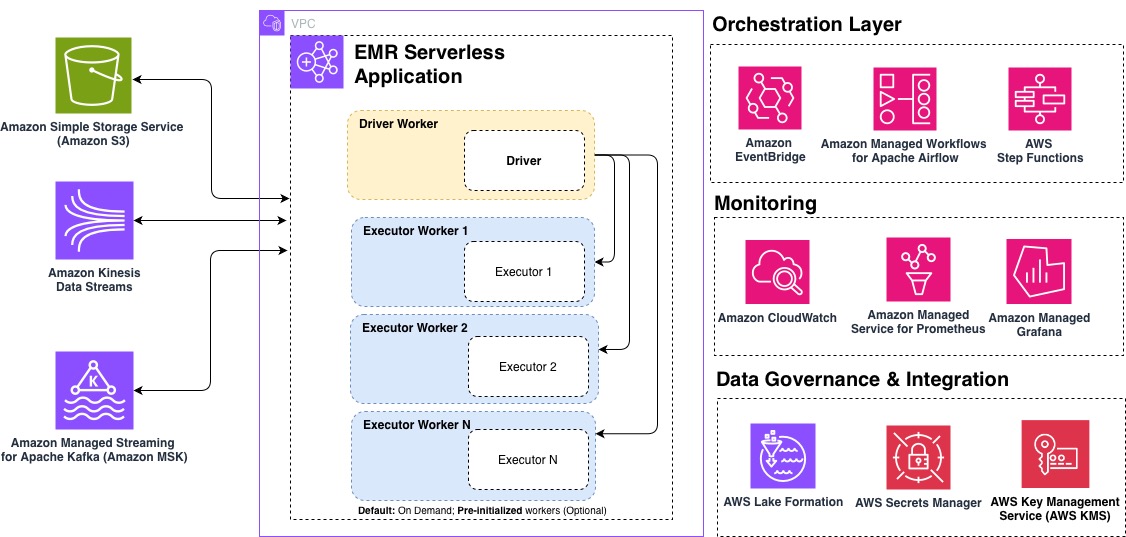
In this post, we share the top 10 best practices for optimizing your EMR Serverless workloads for performance, cost, and scalability. Whether you’re getting started with EMR Serverless or looking to fine-tune existing production workloads, these recommendations will help you build efficient, cost-effective data processing pipelines. The following diagram illustrates an end-to-end EMR Serverless architecture, showing how it integrates into your analytics pipelines.
1. Define applications one time, reuse multiple times

EMR Serverless applications function as cluster templates that instantiate when jobs are submitted and can process multiple jobs without being recreated. This design significantly reduces startup latency for recurring workloads and simplifies operational management.

Typical workflow for EMR on EC2 transient cluster:

Typical workflow for EMR Serverless:

Applications feature a self-managing lifecycle that provisions resources to be available when needed without manual intervention. They automatically provision capacity when a job is submitted. For applications without pre-initialized capacity, resources are released immediately after job completion. For applications with pre-initialized capacity configured, those pre-initialized workers will stop after exceeding the configured idle timeout (15 minutes by default). You can adjust this timeout at the application level using AutoStopConfig configuration in the CreateApplication or UpdateApplication API. For example, if your jobs run every 30 minutes, increasing the idle timeout can eliminate startup delays between executions.

Most workloads are suited for on-demand capacity provisioning, which automatically scales resources based on your job requirements without incurring charges when idle. This approach is cost-effective and suitable for typical use cases including extract, transform, and load (ETL) workloads, batch processing jobs, and scenarios requiring maximum job resiliency.

For specific workloads with strict instant-start requirements, you can optionally configure pre-initialized capacity. Pre-initialized capacity creates a warm pool of drivers and executors that are ready to run jobs within seconds. However, this performance advantage comes with a tradeoff of added cost because pre-initialized workers incur continuous charges even when idle until the application reaches the Stopped state. Additionally, pre-initialized capacity restricts jobs to a single Availability Zone, which reduces resiliency.

Pre-initialized capacity should only be considered for:

  • Time-sensitive jobs with sub second service level agreement (SLA) requirements where startup latency is unacceptable
  • Interactive analytics where user experience depends on instant response
  • High-frequency production pipelines running every few minutes

In most other cases, on-demand capacity provides the best balance of cost, performance, and resiliency.

Beyond optimizing your applications’ use of resources, consider how you organize them across your workloads. For production workloads, use separate applications for different business domains or data sensitivity levels. This isolation improves governance and prevents resource contention between critical and noncritical jobs.

2. Choose AWS Graviton Processors for better price performance

Selecting the right underlying processor architecture can significantly impact both performance and cost. Graviton ARM-based processors offer significant performance improvement compared to x86_64.

EMR Serverless automatically updates to the latest instance generations as they become available, which means your applications benefit from the newest hardware improvements without requiring additional configuration.

To use Graviton with EMR Serverless, specify ARM64 with the architecture parameter during application creation using the CreateApplication or with the UpdateApplication API for existing applications:

aws emr-serverless create-application \
  --name my-spark-app \
  -- SPARK \
  --architecture ARM64 \
  --release-label emr-7.12.0

Considerations when using Graviton:

  • Resource availability – For large-scale workloads, consider engaging with your AWS account team to discuss capacity planning for Graviton workers.
  • Compatibility – Although many commonly used and standard libraries are compatible with Graviton (arm64) architecture, you will need to validate that third-party packages and libraries used are compatible.
  • Migration planning – Take a strategic approach to Graviton adoption. Build new applications on ARM64 architecture by default and migrate existing workloads through a phased transition plan that minimizes disruption. This structured approach will help optimize cost and performance without compromising reliability.
  • Perform benchmarks – It’s important to note that exact price performance will vary by workload. We recommend performing your own benchmarks to gauge specific results for your workload. For more details, refer to Achieve up to 27% better price-performance for Spark workloads with AWS Graviton2 on Amazon EMR Serverless.

3. Use defaults, right-size workers if needed

Workers are used to execute the tasks for your workload. While EMR Serverless defaults are optimized out of the box for a majority of use cases, you may need to right-size your workers to improve processing time and optimize cost efficiency. When submitting EMR Serverless jobs, it’s recommended to define Spark properties to configure workers, including memory size (in GB) and number of cores.

EMR Serverless configures the default worker size of 4 vCPUs, 16 GB memory, and 20 GB disk. Although this generally provides a balanced configuration for most jobs, you might want to adjust the size based on your performance requirements. Even when configuring pre-initialized workers with specific sizing, always set your Spark properties at job submission. This allows your job to use the specified worker sizing rather than default properties when it scales beyond pre-initialized capacity. When right-sizing your Spark workload, it’s important to identify the vCPU:memory ratio for your job. This ratio determines how much memory you allocate per virtual CPU core in your executors. Spark executors need both CPU and memory to process data effectively, and the optimal ratio varies based on your workload characteristics.

To get started, use the following guidance, then refine your configuration based on your specific workload requirements.

Executor configuration

The following table provides recommended executor configurations based on common workload patterns:

Workload type Ratio CPU Memory Configuration
Compute intensive 1:2 16 vCPU 32 GB spark.emr-serverless.executor.cores=16spark.emr-serverless.executor.memory=32G
General purpose 1:4 16 vCPU 64 GB spark.emr-serverless.executor.cores=16spark.emr-serverless.executor.memory=64G
Memory intensive 1:8 16 vCPU 108 GB spark.emr-serverless.executor.cores=16spark.emr-serverless.executor.memory=108G

Driver configuration

The following table provides recommended driver configurations based on common workload patterns:

Workload type Ratio CPU Memory Configuration
General purpose 1:4 4 vCPU 16 GB spark.emr-serverless.driver.cores=4spark.emr-serverless.driver.memory=16G
Apache Iceberg workloads 1:8(Large driver for metadata lookups) 8 vCPU 60 GB spark.emr-serverless.driver.cores=8spark.emr-serverless.driver.memory=60G

To further monitor and tune your configuration, monitor your workload’s resource consumption using Amazon CloudWatch job worker-level metrics to identify constraints. Track CPU utilization, memory usage, and disk utilization metrics, then use the following table to fine-tune your configuration based on observed bottlenecks.

Metrics observed Workload type Suggested action
1 High memory (>90%), Low CPU (<50%) Memory-bound workload Increase vCPU:memory ratio
2 High CPU (>85%), low memory (<60%) CPU-bound workload Increase vCPU count, maintain 1:4 ratio (For example, if using 8 vCPU, use 32 GB memory)
3 High storage I/O, normal CPU or memory with long shuffle operations Shuffle-intensive Enable serverless storage or shuffle-optimized disks
4 Low utilization across metrics Over-provisioned Reduce worker size or count
5 Consistent high utilization (>90%) Under-provisioned Scale up worker specifications
6 Frequent GC pauses** Memory pressure Increase memory overhead (10 –15%)

**You can identify frequent garbage collect (GC) pauses using the Spark UI under the Executors tab. There will be a GC time column that should generally be less than 10% of task time. Alternatively, the driver logs might frequently contain GC (Allocation Failure)] messages.

4. Control scaling boundary with T-shirt sizing

By default, EMR Serverless uses dynamic resource allocation (DRA), which automatically scales resources based on workload demand. EMR Serverless continuously evaluates metrics from the job to optimize for cost and speed, removing the need for you to estimate the exact number of workers required.

For cost optimization and predictable performance, you can configure an upper scaling boundary using one of the following approaches:

  1. Setting the spark.dynamicAllocation.maxExecutors parameter at the job level
  2. Setting the application-level maximum capacity

Rather than trying to fine-tune spark.dynamicAllocation.maxExecutors to an arbitrary value for each job, you can think about setting this configuration as t-shirt sizes that represent different workload profiles:

Workload size Use cases spark.dynamicAllocation.maxExecutors
Small Exploratory queries, development 50
Medium Regular ETL jobs, reports 200
Large Complex transformations, large-scale processing 500

This t-shirt sizing approach simplifies capacity planning and helps you balance performance with cost efficiency based on your workload category, rather than attempting to optimize each individual job.

For EMR Serverless releases 6.10 and above, the default value for spark.dynamicAllocation.maxExecutors is infinity, but for earlier releases, it’s 100.

EMR Serverless automatically scales workers up or down based on the workload and parallelism required at every stage of the job. This automatic scaling is continuously evaluating metrics from the job to optimize for cost and speed, which removes the need for you to estimate the number of workers that the application needs to run your workloads.

However, in some cases, if you have a predictable workload, you might want to statically set the number of executors. To do so, you can disable DRA and specify the number of executors manually:

spark.dynamicAllocation.=false
spark.executor.instances=10

5. Provision appropriate storage for EMR Serverless jobs

Understanding your storage options and sizing them appropriately can prevent job failures and optimize execution times. EMR Serverless offers multiple storage options to handle intermediate data during job execution. The storage option selected will depend on the EMR release and use case. The storage options available in EMR Serverless are:

Storage type EMR release Disk size range Use case Benefits
Serverless Storage (recommended) 7.12+ N/A (auto-scaling) Most Spark workloads, especially data-intensive workloads
  • No storage costs
  • auto-scaling
  • Reduces disk failures
  • Up to 20% cost reduction
Standard Disks 7.11 and lower 20–200 GB per worker Small to medium workloads processing datasets under 10 TB
  • Simple configuration
  • 20 GB default suitable for most workloads,
  • 200 GB max for optimal throughput
Shuffle-Optimized Disks 7.1.0+ 20–2,000 GB per worker Large-scale ETL workloads processing multi-TB
  • High IOPS and throughput
  • Up to 2 TB capacity per worker

By matching your storage configuration to your workload characteristics, you’ll enable EMR Serverless jobs to run efficiently and reliably at scale.

6. Multi-AZ out-of-the-box with built-in resiliency

EMR Serverless applications are multi-AZ from the start when pre-initialized capacity isn’t enabled. This built-in failover capability provides resilience against Availability Zone disruptions without manual intervention. A single job will operate within a single Availability Zone to prevent cross-AZ data transfer costs and subsequent jobs will be intelligently distributed across multiple AZs. If EMR Serverless determines that an AZ is impaired, it will submit new jobs to a healthy AZ, enabling your workloads to continue running despite AZ impairment.

To fully benefit from EMR Serverless multi-AZ functionality verify the following:

  • Configure a network connection to your VPC with multiple subnets across Availability Zones selected
  • Avoid pre-initialized capacity which restricts applications to a single AZ
  • Make sure there are sufficient IP addresses available in each subnet to support the scaling of workers

In addition to multi-AZ, with Amazon EMR 7.1 and higher, you can enable job resiliency, which allows your jobs to be automatically retried in case errors are encountered. If there are multiple Availability Zones configured, it will also be retried in a different AZ. You can enable this feature for both batch and streaming jobs, though retry behavior differs between the two.

Configure job resiliency by specifying a retry policy that defines the maximum number of retry attempts. For batch jobs, the default is no automatic retries (maxAttempts=1). For streaming jobs, EMR Serverless retries indefinitely with built-in thrash prevention that stops retries after five failed attempts within 1 hour. You can configure this threshold between 1–10 attempts. For more information, refer to Job resiliency.

In the event that you need to cancel your job, you can specify a grace period to allow your jobs to shut down cleanly rather than the default behavior of immediate termination. This can also include custom shutdown hooks if you need to perform custom cleanup actions.

By combining multi-AZ support, automatic job retries, and graceful shutdown periods, you create a robust foundation for EMR Serverless workloads that can tolerate interruptions and maintain data integrity without manual intervention.

7. Secure and extend connectivity with VPC integration

By default, EMR Serverless can access AWS services such as Amazon Simple Storage Service (Amazon S3), AWS Glue, Amazon CloudWatch Logs, AWS Key Management Service (AWS KMS), AWS Security Token Service (AWS STS), Amazon DynamoDB, and AWS Secrets Manager. If you want to connect to data stores within your VPC, such as Amazon Redshift or Amazon Relational Database Service (Amazon RDS), you must configure VPC access for the EMR Serverless application.

When configuring VPC access for your EMR Serverless application, keep these key considerations in mind to gain optimal performance and cost efficiency:

  • Plan for sufficient IP addresses – Each worker uses one IP address within a subnet. This includes the workers that will be launched when your job is scaling out. If there aren’t enough IP addresses, your job might not be able to scale, which could result in job failure. Verify you have adhered to best practices for subnet planning for optimal performance.
  • Set up Gateway endpoints for Amazon S3 for applications in a private subnets – Running EMR Serverless in a private subnet without VPC endpoints for Amazon S3 will route your Amazon S3 traffic through NAT gateways, resulting in additional data transfer charges. VPC endpoints for S3 will keep this traffic within your VPC, reducing costs and improving performance for Amazon S3 operations.
  • Manage AWS Config costs for network interfaces – EMR Serverless generates an elastic network interface record in AWS Config for each worker, which can accumulate costs as your workloads scale. If you don’t require AWS Config tracking for EMR Serverless network interfaces, consider using resource-based exclusions or tagging strategies to filter them out while maintaining AWS Config coverage for other resources.

For more details, refer Configuring VPC access for EMR Serverless applications.

8. Simplify job submission and dependency management

EMR Serverless supports flexible job submission through the StartJobRun API, which accepts the full spark-submit syntax. For runtime environment configuration, use the spark.emr-serverless.driverEnv and spark.executorEnv prefixes to set environment variables for driver and executor processes. This is particularly useful for passing sensitive configuration or runtime-specific settings.

For Python applications, package dependencies using virtual environments by creating a venv, packaging it as a tar.gz archive, or uploading to Amazon S3 using spark.archives with the appropriate PYSPARK_PYTHON environment variable. This allows Python dependencies to be available across driver and executor workers.

For improved control under high load, enable job concurrency and queuing (available in EMR 7.0.0+) to limit the number of jobs that can be executed concurrently. With this feature, jobs submitted that exceed the concurrency limit are queued until resources become available.

You can configure Job concurrency and queue settings using the SchedulerConfiguration property using the CreateApplication or UpdateApplication API.

--scheduler-configuration '{"maxConcurrentRuns": 5, "queueTimeoutMinutes": 30}'

9. Use EMR Serverless configurations to enforce limits

EMR Serverless automatically scales resources based on workload demand, providing optimized defaults that work well for most use cases without requiring Spark configuration tuning. To manage costs effectively, you can configure resource limits that align with your budget and performance requirements. For advanced use cases, EMR Serverless also provides configuration options so you can fine-tune resource consumption and achieve the same efficiency as cluster-based deployments. Understanding these limits helps you balance performance with cost efficiency for your jobs.

Limit type Purpose How to configure
Job-level Control resources for individual jobs spark.dynamicAllocation.maxExecutors or spark.executor.instances
Application-level Limit resources per application or business domain Set maximum capacity when creating the application or while updating.
Account-level Prevent abnormal resource spikes across all applications Auto-adjustable service quota Max concurrent vCPUs per account; request increases via Service Quotas console

These three layers of limits work together to provide flexible resource management at different scopes. For most use cases, configuring job-level limits using the t-shirt sizing approach is sufficient, while application and account-level limits provide additional guardrails for cost control.

10. Monitor with CloudWatch, Prometheus, and Grafana

Monitoring EMR Serverless workloads simplifies the process of debugging, performing cost optimization, and performance tracking. EMR Serverless offers three tiers of monitoring that work together: Amazon CloudWatch, Amazon Managed Service for Prometheus, and Amazon Managed Grafana.

  1. Amazon CloudWatch – CloudWatch integration is enabled by default and publishes metrics to the AWS/EMRServerless namespace. EMR Serverless sends metrics to CloudWatch every minute at the application level, as well as job, worker-type, and capacity-allocation-type levels. Using CloudWatch, you can configure dashboards for enhanced observability into workloads or configure alarms to alert for job failures, scaling anomalies, and SLA breaches. Using CloudWatch with EMR Serverless provides insights to your workloads so you can catch issues before they impact users.
  2. Amazon Managed Service for Prometheus – With EMR Serverless release 7.1+, you can enable Prometheus for detailed Spark engine metrics to push metrics to Amazon Managed Service for Prometheus. This unlocks executor-level visibility, including memory usage, shuffle volumes, and GC pressure. You can use this to identify memory-constrained executors, detect shuffle-heavy stages, and find data skew.
  3. Amazon Managed Grafana – Grafana connects to both CloudWatch and Prometheus data sources, providing a single pane of glass for unified observability and correlation analysis. This layered approach helps you correlate infrastructure issues with application-level performance problems.

Key metrics to track:

  • Job completion times and success rates
  • Worker utilization and scaling events
  • Shuffle read/write volumes
  • Memory usage patterns

For more details, refer to Monitor Amazon EMR Serverless workers in near real time using Amazon CloudWatch.

Conclusion

In this post, we shared 10 best practices to help you maximize the value of Amazon EMR Serverless by optimizing performance, controlling costs, and maintaining reliable operations at scale. By focusing on application design, right-sized workloads, and architectural choices, you can build data processing pipelines that are both efficient and resilient.

To learn more, refer to the Getting started with EMR Serverless guide.

About the Authors

Karthik Prabhakar

Karthik Prabhakar

Karthik is a Data Processing Engines Architect for Amazon EMR at Amazon Web Services (AWS). He specializes in distributed systems architecture and query optimization, working with customers to solve complex performance challenges in large-scale data processing workloads. His focus spans engine internals, cost-optimization strategies, and architectural patterns that enable customers to run petabyte-scale analytics efficiently.

Neil Mukerje

Neil Mukerje

Neil is a Principal Product Manager at Amazon Web Services.

Amber Runnels

Amber Runnels

Amber is a Senior Analytics Specialist Solutions Architect at Amazon Web Services (AWS) specializing in big data and distributed systems. She helps customers optimize workloads within AWS data offerings to achieve a scalable, high-performing, and cost-effective architecture. Aside from technology, she’s passionate about exploring the many places and cultures this world has to offer, reading novels, and building terrariums.

Parul Saxena

Parul Saxena

Parul is a Senior Big Data Specialist Solutions Architect at Amazon Web Services (AWS). She helps customers and partners build highly optimized, scalable, and secure solutions. She specializes in Amazon EMR, Amazon Athena, and AWS Lake Formation, providing architectural guidance for complex big data workloads and assisting organizations in modernizing their architectures and migrating analytics workloads to AWS.

Access a VPC-hosted Amazon OpenSearch Service domain with SAML authentication using AWS Client VPN

Post Syndicated from Jan Michael Go Tan original https://aws.amazon.com/blogs/big-data/access-a-vpc-hosted-amazon-opensearch-service-domain-with-saml-authentication-using-aws-client-vpn/

Customers often want to deploy Amazon OpenSearch Service domains in virtual private clouds (VPC) and use single sign-on (SSO) with SAML for access control to enhance security. However, setting this up can be challenging.

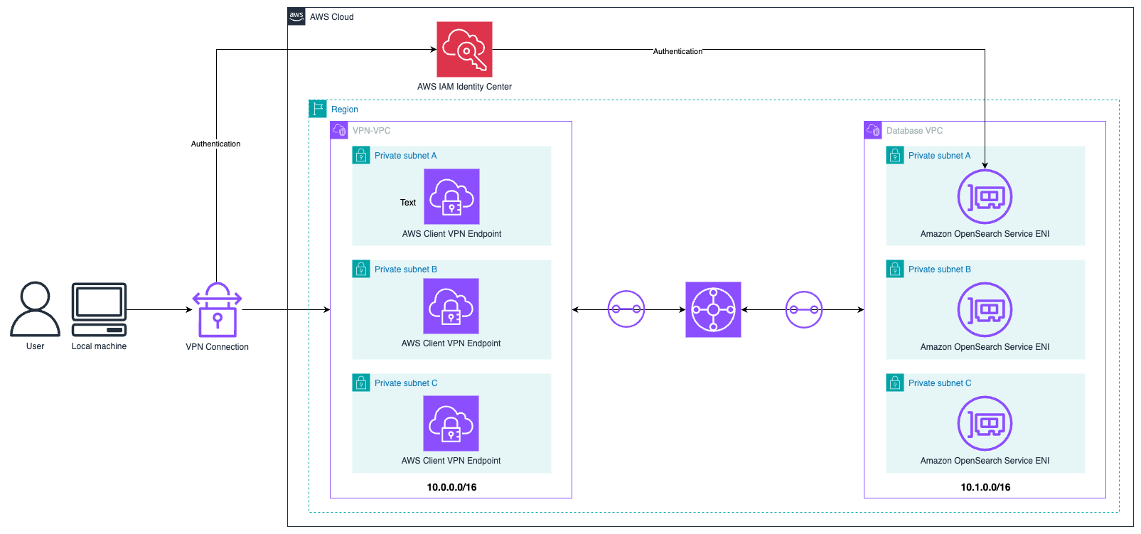
In this post, we explore different OpenSearch Service authentication methods and network topology considerations. Then we show how to build an architecture to access an OpenSearch Service domain hosted in a VPC using AWS Client VPN, AWS Transit Gateway, and AWS IAM Identity Center.

Solution overview

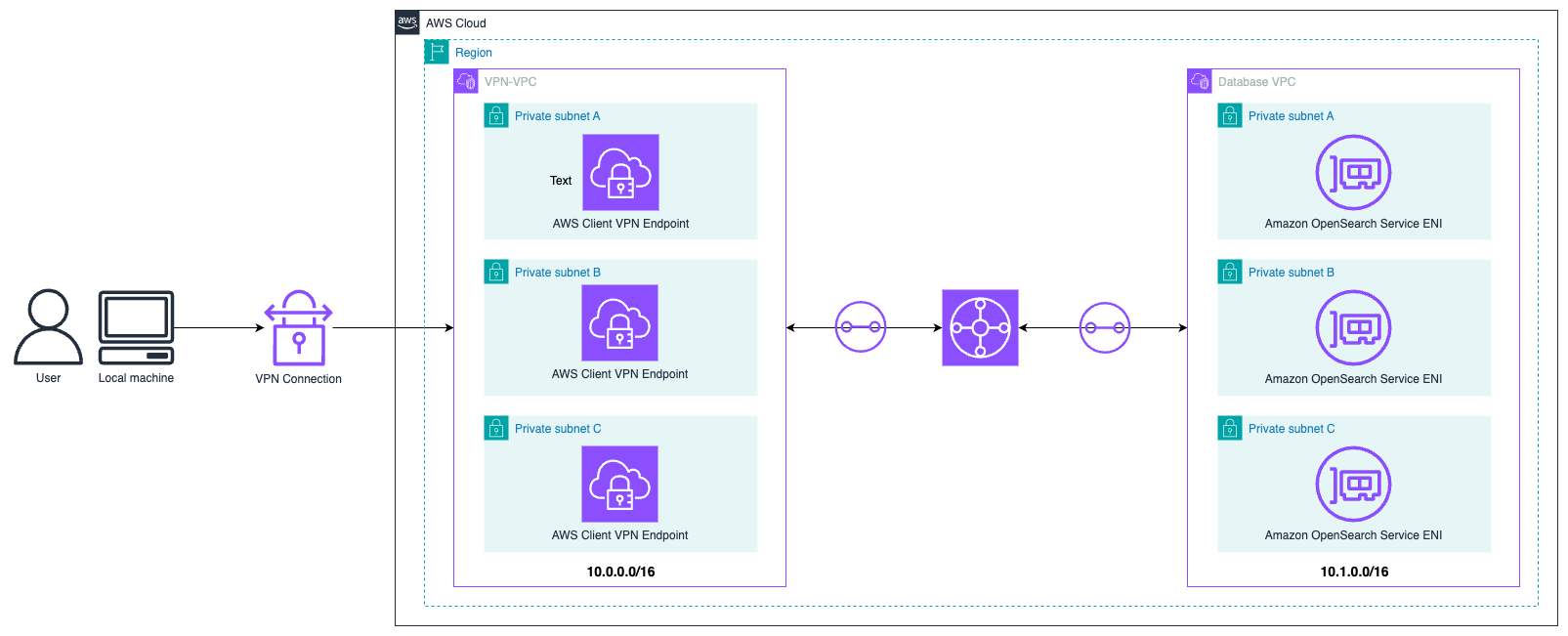
The following diagram illustrates the solution architecture.

High-level network diagram

The end-user authenticates with IAM Identity Center and connects to the AWS environment from their browser through Client VPN. The traffic is routed from the VPN VPC to the database VPC where the OpenSearch service endpoints are deployed. The user then authenticates to OpenSearch Service through IAM Identity Center. This architecture provides a scalable, enterprise-grade solution that avoids using bastion hosts while making sure only authorized users can access your OpenSearch Service domains through a secure VPN connection. In the following sections, we walk through the steps to set up IAM Identity Center, configure Transit Gateway to facilitate communication between VPCs, and configure SAML-based authentication using IAM Identity Center for both OpenSearch Service and VPN access. Prior experience setting up Client VPN, IAM Identity Center, and Transit Gateway would be beneficial but is not necessary to follow along with this post.

OpenSearch Service authentication methods and SAML

OpenSearch Service supports multiple authentication methods. You can use AWS Identity and Access Management (IAM) to call the OpenSearch Service configuration API (for details, see Making and signing OpenSearch Service requests). However, this doesn’t give you access to the visual dashboard. To access the visual dashboard and call the OpenSearch Service configuration API, you can use the OpenSearch Service built-in internal user database or Amazon Cognito for authentication and user management features. However, these options use separate user pools, which adds additional security and management overhead when adding and removing users.

Therefore, many customers choose to use SAML federation to integrate OpenSearch Service authentication with their existing identity providers like Entra ID, Okta, or JumpCloud. For this post, we use the IAM Identity Center directory as our identity source. One limitation of this approach is that it only supports identity provider-initiated authentication. This means that users must log in through the IAM Identity Center portal and then access their OpenSearch Service dashboard from there.

Private network topology options for OpenSearch Service

When deploying OpenSearch Service domains in a private VPC, organizations must establish secure and reliable network connectivity to access their OpenSearch Service domains. AWS offers several networking solutions that can be implemented individually or in combination to meet specific access requirements. These options include Transit Gateway for centralized network management, AWS Direct Connect or AWS Site-to-Site VPN for on-premises connectivity, and Client VPN for secure remote access. Each solution provides unique benefits and can be combined to meet different organizational needs, security requirements, and performance expectations.

AWS Transit Gateway

Transit Gateway functions as a cloud router that simplifies network connectivity by acting as a central hub for connecting VPCs and on-premises networks. Implementing Transit Gateway with OpenSearch Service enables consolidated access to your OpenSearch Service domain across multiple VPCs and AWS accounts. Through Transit Gateway route tables, you can precisely control traffic flow between attached networks. It supports transitive routing between VPCs and on-premises networks, significantly reducing the number of peering connections needed to access your OpenSearch Service domain. This centralized approach is a common pattern used by customers, which makes network management scalable as your infrastructure grows.

AWS Client VPN

With Client VPN, you can securely access your private OpenSearch Service domain through a managed OpenVPN-based solution. Using Client VPN removes the need to use a bastion host or proxy server to access an OpenSearch Service domain, reducing your management burden and improving security. Client VPN supports both certificate-based and SAML-based authentication. Client VPN endpoints can be associated with multiple subnets to provide high availability. The service includes comprehensive security features such as connection logging and security group controls.

For more information on VPC connectivity options, refer to the AWS Direct Connect whitepaper.

Combining Client VPN with Transit Gateway provides a scalable and flexible way to access an OpenSearch Service domain in a private VPC. In the subsequent sections, we walk you through how to integrate the various services.

Prerequisites

If you haven’t yet set up IAM Identity Center, refer to Enable IAM Identity Center to enable it. Both organization instances and account instances will work. The Identity Center instance must be deployed in the same AWS Region as your OpenSearch Service domain.

After you set up IAM Identity Center, complete the following steps to create an IAM Identity Center group:

  1. On the IAM Identity Center console, choose Groups in the navigation pane.
  2. Choose Create group and create a group (for this example, we name the group vpn_users.
  3. After you create the group, choose the group name to open its details page.
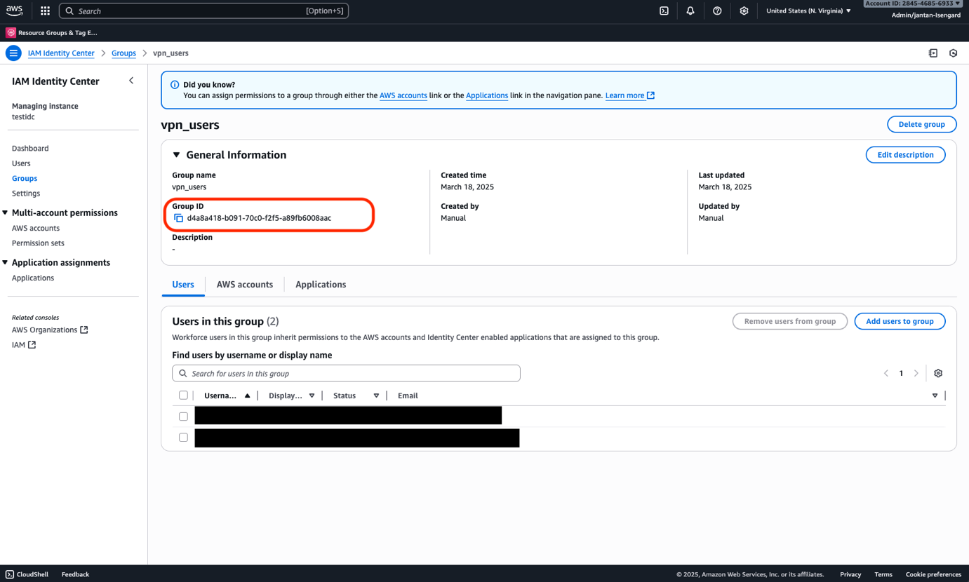
  4. Locate the group ID under General information. Save this in a text editor.
    IAM Identity Center Group ID
  5. Create a user (or multiple users) and assign them to the vpn_users group. This can be done directly through the user creation flow or after creating the user.

Set up the initial network topology

For this post, we use the network topology shown in the following diagram. One VPC hosts the client VPN endpoint with CIDR range 10.0.0.0/16 and a separate VPC with CIDR range 10.1.0.0/16 that hosts our OpenSearch Service nodes. The two VPCs are connected with Transit Gateway. The CIDR ranges in your environment may vary. The only requirement is that they can’t overlap.

Network topology

Complete the following steps to create the two VPCs using Amazon Virtual Private Cloud (Amazon VPC):

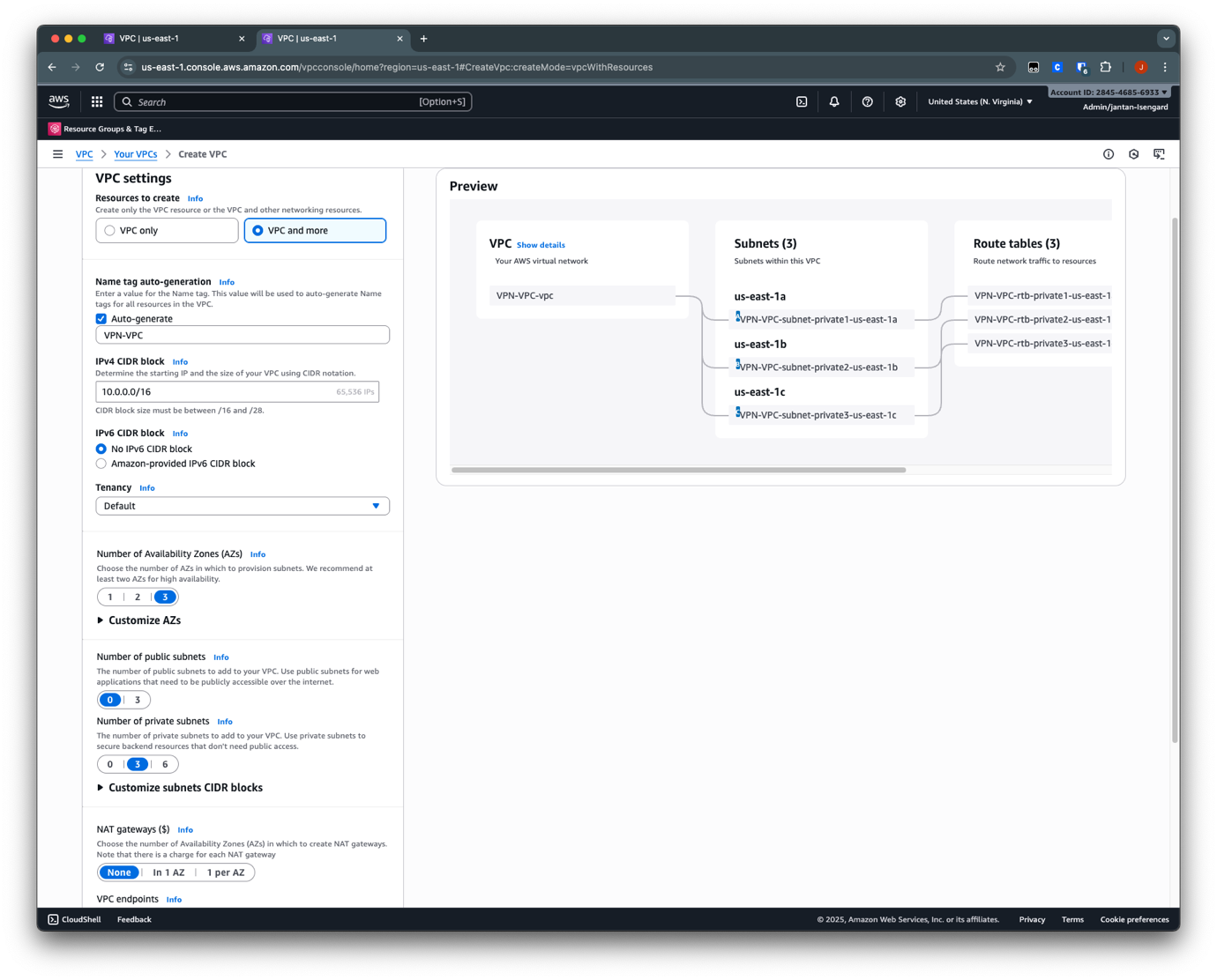
  1. On the Amazon VPC console, choose Create VPC.
  2. Choose VPC and more.
  3. For this post, name the VPC VPN-VPC and use 10.0.0.0/16 for the IPv4 CIDR block.
  4. Choose 3 for the number of Availability Zones.
  5. Choose 0 for the number of public subnets.
  6. Choose 3 for the number of private subnets.
  7. Choose None for the number of NAT gateways.
  8. Choose None for the number of VPC endpoints.
    Initial VPC configuration
  9. Repeat these steps to create the second VPC for the OpenSearch Service domain. Keep the same configuration settings except for the following:
    1. Name: Database-VPC
    2. IPv4 CIDR Block: 10.1.0.0/16

Configure Transit Gateway

Follow the instructions in Create an AWS Transit Gateway using the Amazon VPC Console to create a transit gateway and attach your VPCs to it.

Next, you must update each VPC route table to facilitate connectivity to the OpenSearch Service domain.

  1. On the Amazon VPC console, choose Route tables in the navigation pane.
  2. For VPN-VPC, add routes on the subnets where the Client VPN endpoints are attached. The route is 10.1.0.0/16 using Transit Gateway. This route allows VPN users to reach Database-VPC.
    Route table
  3. For Database-VPC, add routes on the subnets of the OpenSearch Service domain endpoint. The route is 10.0.0.0/16 using Transit Gateway. This route allows responses from Database-VPC back to reach the VPN users.
    OpenSearch Route Table

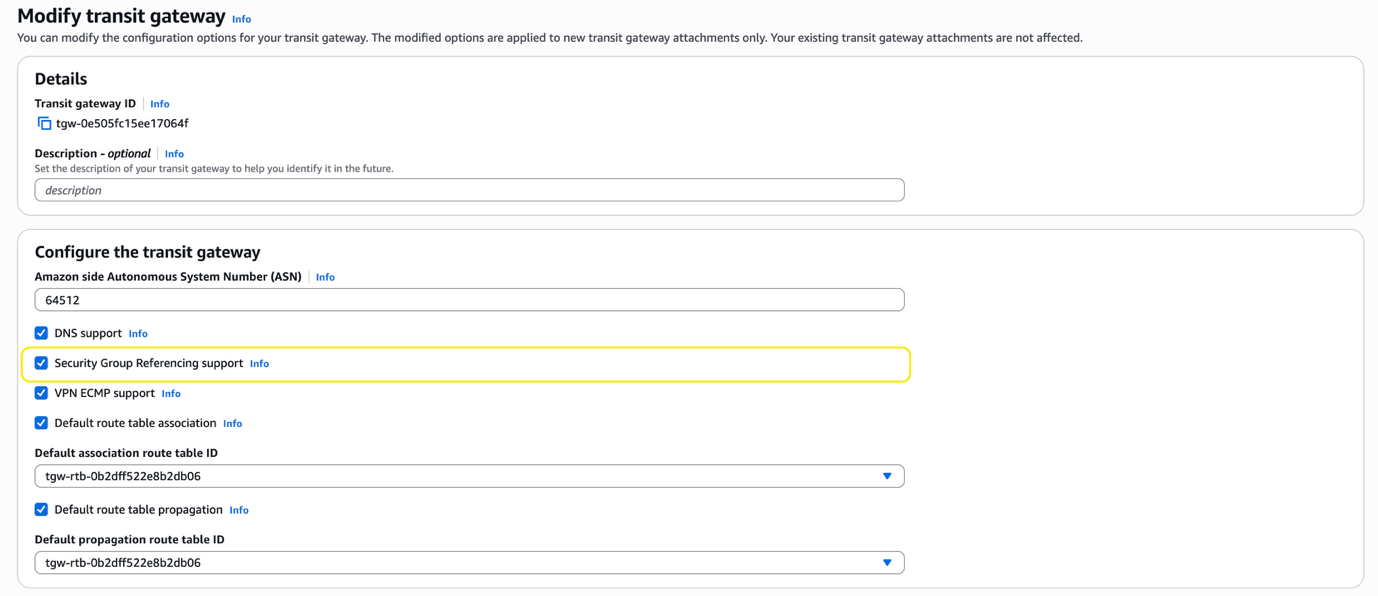
    Next, you must update the Transit Gateway Security Group Referencing support configuration. This allows the OpenSearch Service domain’s security group to open port 443 to only the Client VPN security group. This makes applying least privilege simpler.

  4. On the Transit Gateway console, select the transit gateway you’re using.
  5. On the Actions menu, choose Modify transit gateway.
    Modify TGW
  6. Select Security Group Referencing support and choose Modify transit gateway.
    TGW Security Group Configuration

Configure Client VPN authentication

Client VPN can be associated to multiple VPC subnets for high availability. Client VPN supports multiple client authentication methods. For this post, we use SAML-based authentication with IAM Identity Center.

To set up SAML-based authentication with IAM Identity Center, follow the instructions in the following sections. For more details, refer to Authenticate AWS Client VPN users with AWS IAM Identity Center. Deploy and associate the Client VPN endpoint with VPN-VPC.

Configure Client VPN access to database VPC

During the initial setup of the Client VPN endpoint, you defined authorization rules that authorized the VPN_users group to access the VPN-VPC network, which is 10.0.0.0/16.Complete the following steps to add connectivity to database-VPC:

  1. On the Amazon VPC console, choose Client VPC endpoints in the navigation pane.
  2. Select the endpoint you created.
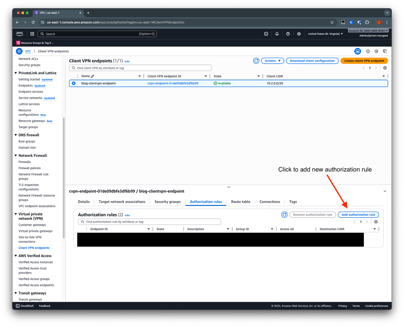
  3. In the Authorization rules section, choose Add authorization rules.
    ClientVPN Auth Rules
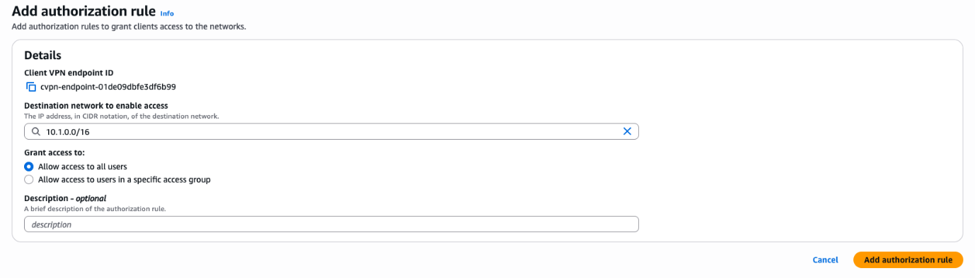
  4. For Destination network to enable access, enter 10.1.0.0/16 (this is the database VPC).
  5. For Grant access to, select Allow access to all users.
  6. Choose Add authorization rule.
    ClientVPN Add Auth Rule

    After you create the authorization rule, the user now has access to that CIDR range. Next, you add an entry in the Client VPN endpoint’s route table to provide reachability from a network perspective.

  7. On the Client VPN endpoints page, select the endpoint you just created.
  8. In the Route table section, choose Create route.
    ClientVPN Route
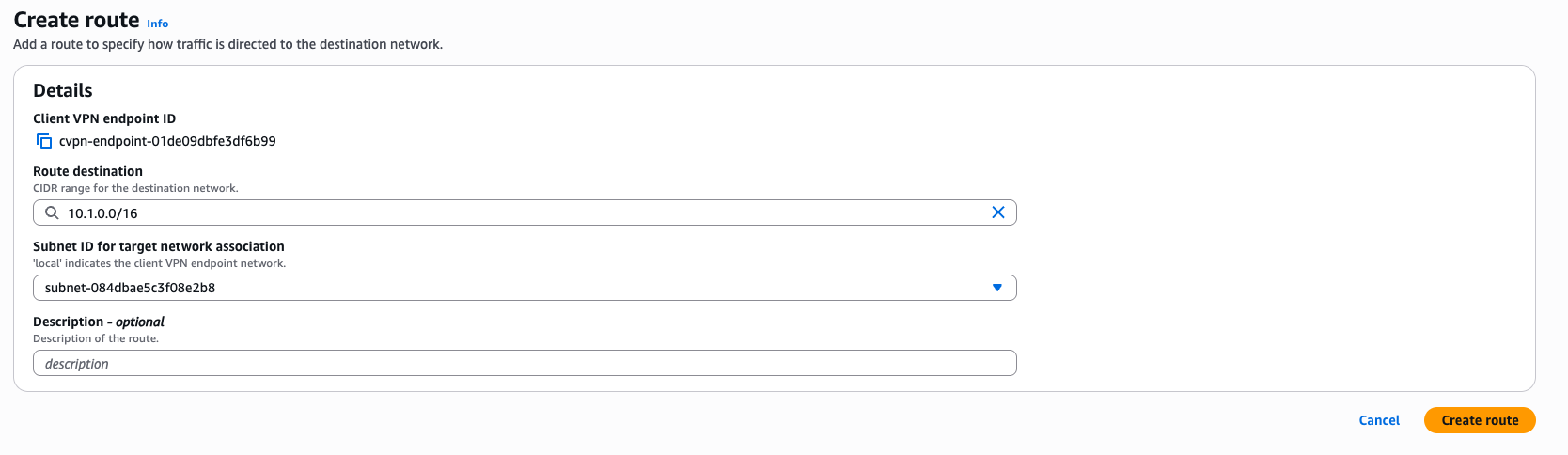
  9. For Route destination, enter the CIDR range for Database-VPC (10.1.0.0/16).
  10. For Subnet ID for target network association, choose a subnet ID.
  11. Choose Create route.
    ClientVPN Create Route

You should see the new route in the “Creating” state. After it has reached the “Active” state, VPN users will have a network path to the database VPC to be able to reach the OpenSearch Service domain.

ClientVPN Route Creating State

Configure Client VPN application on your client

Complete the following steps to configure the Client VPN application to your client:

  1. Download the relevant installer for Client VPN for Desktop and install Client VPN.
  2. Download and prepare the Client VPN endpoint file.
  3. Open the Client VPN application.
  4. Choose Manage Profile, then choose Add Profile.
  5. Enter a display name and upload the VPN configuration file.
  6. Choose Add Profile.

Set up federation with IAM Identity Center with OpenSearch Service

Complete the following steps to set up federation with IAM Identity Center with OpenSearch Service:

  1. Create an OpenSearch Service domain in the database VPC.
  2. Set up the SAML integration between OpenSearch Service and IAM Identity Center. Assign the same groups that you assigned to the VPN custom application to the OpenSearch Service custom application.
  3. Modify the security group associated with the OpenSearch Service domain to allow access from the Client VPN subnet.
  4. Modify the security group of Client VPN and add the following entry:
    1. Type: HTTPS
    2. Source: Use Custom and reference the security group of the OpenSearch Service domain

Test the end-to-end flow

Now you can test the entire flow end-to-end:

  1. Run Client VPN on your local machine. Use the profile that you previously configured.
    The client will prompt you to authenticate with IAM Identity Center. After authentication, you will see the message “Authentication details received, processing details. You may close this window at any time.”
  2. Access your IAM Identity Center access portal URL (this can be found on the IAM Identity Center console, under Dashboard). Sign in as a user that has been assigned to the OpenSearch Service custom application in the previous step.
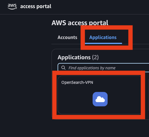
  3. After authentication, choose the Applications tab in AWS Access Portal and choose the OpenSearch Service application.

This should redirect you to the OpenSearch Service Dashboards page with the role that you assigned.

IAM Identity Center - App List

Clean up

After you test the solution, delete the resources you created to avoid incurring future charges:

  1. Delete the OpenSearch Service domain and the SAML application, users, and groups in IAM Identity Center.
  2. Delete the client VPN endpoints that you created and remove the routing rules from Transit Gateway.

Conclusion

In this post, we discussed the networking options for securely accessing an OpenSearch Service domain deployed in a private VPC through services like Transit Gateway, Client VPN, and Site-to-Site VPN. We also discussed how to use IAM Identity Center for authentication and authorization, helping you simplify identity management for OpenSearch Service. If you have feedback about this post, provide it in the comments section.


About the authors

Jan Michael Go Tan

Jan Michael Go Tan

Jan Michael is a Principal Solutions Architect for Amazon Web Services. He helps customers design scalable and innovative solutions with the AWS Cloud.

Kevin Low

Kevin Low

Kevin is a Security Solutions Architect at AWS who helps the largest customers across ASEAN build securely. He specializes in threat detection and incident response and is passionate about integrating resilience and security. Outside of work, he loves spending time with his wife and dog, a poodle called Noodle.

Enable strategic data quality management with AWS Glue DQDL labels

Post Syndicated from Arun A K original https://aws.amazon.com/blogs/big-data/enable-strategic-data-quality-management-with-aws-glue-dqdl-labels/

Organizations increasingly depend on trusted, high-quality data to drive analytics, regulatory reporting, and operational decision-making. When data quality issues go undetected, they can lead to inaccurate insights, stalled initiatives, and compliance gaps that directly affect business outcomes. As data volumes grow and pipelines become more distributed, maintaining consistent data quality across teams and data domains becomes progressively more challenging.

You can address these challenges with AWS Glue Data Quality by providing automated, rule-based data validation across datasets in the AWS Glue Data Catalog and within AWS Glue ETL pipelines. With the Data Quality Definition Language (DQDL), you can author both straightforward and advanced validation rules to detect data quality issues early in the lifecycle, before they reach downstream applications or analytics environments.

In this post, we highlight the new DQDL labels feature, which enhances how you organize, prioritize, and operationalize your data quality efforts at scale. We show how labels such as business criticality, compliance requirements, team ownership, or data domain can be attached to data quality rules to streamline triage and analysis. You’ll learn how to quickly surface targeted insights (for example, “all high-priority customer data failures owned by marketing” or “GDPR-related issues from our Salesforce ingestion pipeline”) and how DQDL labels can help teams improve accountability and accelerate remediation workflows.

Managing complex data quality rules across teams and use cases

As organizations advance in their data quality programs, a few rules often grow into hundreds or thousands maintained across many teams and business domains. Take the example of AnyCompany, a large retail organization with multiple data teams managing customer, product, and sales data across different business units. These teams run a variety of data quality rules, including weekly customer checks, daily product validations, frequent sales checks, and monthly compliance reviews, with different naming patterns, schedules, and response processes. This creates a fragmented, hard-to-navigate system where teams operate in isolation and data quality practices become inconsistent.

The challenge lies in the volume of rules and the lack of organizational context around them. When dozens of data quality rules pass or fail, teams still lack clarity on ownership, urgency, or business impact. This slows incident response, limits executive insight, and complicates resource planning. To move from technical monitoring to strategic value, organizations need a unified structure that connects data quality rules to teams, domains, and priorities, bringing essential business context to data quality operations.

Metadata-driven rule organization

AWS Glue DQDL labels address organizational challenges because you can attach custom metadata to data quality rules, transforming anonymous validations into contextually rich, business-aware checks. Labels work as key-value pairs attached to individual rules or entire rule sets, and you can organize quality operations around business dimensions such as team ownership, criticality, frequency, and regulatory requirements, as in the case of the AnyCompany example. When a rule fails, you immediately identify what failed, who should respond, how urgent it is, and which business area is affected, whether it’s the marketing department tracking email completeness with daily frequency tags, compliance teams monitoring age verification with regulation labels, or the finance team validating payment data with high-criticality markers.

Labels integrate with existing DQDL syntax without requiring changes to current rule definitions, working consistently across AWS Glue Data Quality execution contexts. The feature’s flexibility supports organizational taxonomies from cost centers and geographic regions to data sensitivity levels and service-level agreement (SLA) requirements with single rules carrying multiple labels simultaneously for sophisticated filtering and analysis. Labels appear in the outputs, including rule outcomes, row-level results, and API responses, so organizational context travels with quality results whether you’re troubleshooting failures, analyzing trends in Amazon Athena, or building executive dashboards in Amazon Quick Sight.

Getting started: Writing your first labeled data quality rules

Let’s walk through creating your first labeled data quality rules using AnyCompany’s customer data scenario. We’ll use their customer demographics dataset, which contains customer information that multiple teams need to validate with different priorities and frequencies.

DQDL labels follow a straightforward key-value pair syntax that integrates naturally with existing rule definitions. The basic syntax supports two approaches: default labels that apply to the rules in a rule set, and rule-specific labels that apply to individual rules. Rule-specific labels can override default labels when using the same key, providing fine-grained control over your labeling strategy.

When implementing DQDL labels, keep the following constraints in mind:

  • Maximum of 10 labels per rule
  • Label keys are limited to 128 characters and can’t be empty
  • Label values are limited to 256 characters and can’t be empty
  • Both keys and values are case-sensitive
  • Rule-specific labels override default labels when using the same key

Using this labeling approach, you can organize and manage data quality rules efficiently across different teams and validation requirements.

Best practices for label naming conventions

Here are some proven labeling strategies that scale across enterprise environments:

  • Establish a complete standardized taxonomy upfront – Define label keys in DefaultLabels with sensible defaults such as regulation=none or sla=24h to provide rules with identical keys for cross-team queries.
  • Use consistent key naming patterns – Establish standard keys such as team, criticality, sla, impact, and regulation across rule sets to maintain query consistency.
  • Implement hierarchical values – Use formats such as team=marketing-analytics to support both broad and specific filtering while keeping key structure consistent.
  • Include operational metadata in defaults – Define labels such as sla, escalation-level, or notification-channel as defaults to drive automated response workflows.
  • Plan for reporting dimensions – Include keys such as cost-center, region, or business-unit in your default taxonomy to support meaningful business analytics.
  • Use standardized value patterns – Establish consistent formats such as criticality=high/medium/low or sla=15m/1h/1d for predictable filtering and sorting.

These are guidelines rather than requirements but following them from the start enables powerful cross-team analytics and reduces future refactoring effort.

Customer data validation hands-on example

This post assumes you’re familiar with AWS Glue Data Quality and ETL operations. Using the following hands-on walkthrough, you’ll learn how to implement DQDL labels for organizational data quality management.

Start by establishing default labels that automatically apply to every rule in the rule set, providing consistent organizational context:

DefaultLabels = ["team"="data-team", "criticality"="medium", "regulation"="none", "sla"="24h", "impact"="medium"]

DefaultLabels provide a foundational taxonomy that automatically propagates across your entire rule set, creating uniformity and reducing configuration overhead. By defining default values at the organizational level, such as team=data-team, criticality=medium, regulation=none, sla=24h, and impact=medium, every rule inherits these standardized attributes without requiring explicit declaration. This inheritance model promotes consistency while maintaining the flexibility individual teams need to address their unique operational contexts.

Individual teams can selectively override inherited defaults to reflect their specific requirements. For example, examine the following complete rule set:

DefaultLabels = ["team"="data-team", "criticality"="medium", "regulation"="none", "sla"="24h", "impact"="medium"]

Rules = [
    IsComplete "c_customer_id" labels=["team"="analytics", "criticality"="high", "sla"="15m", "impact"="high"],
    ColumnValues "c_customer_id" matches "e.*" labels=["team"="analytics", "criticality"="medium", "impact"="low"],
    ColumnLength "c_city" > 6 labels=["team"="marketing", "criticality"="medium", "sla"="4h", "impact"="medium"],
    IsComplete "c_name" labels=["team"="marketing", "sla"="4h"],
    ColumnValues "c_age" >= 21 labels=["team"="compliance", "criticality"="high", "regulation"="age21", "impact"="high"] with threshold > 0.99,
    IsComplete "c_birth_date" labels=["team"="compliance", "criticality"="medium", "regulation"="gdpr", "impact"="medium"],
    IsComplete "c_creditissuer" labels=["team"="finance", "impact"="high"],
    ColumnValues "c_creditcardnumber" > 100000000000 labels=["team"="finance", "criticality"="high", "regulation"="payment", "impact"="high"] with threshold > 0.95
]

Notice how the compliance team changes regulation from 'none' to 'age21' for age verification rules and analytics elevates criticality to 'high' for business-critical checks. Unspecified labels automatically inherit the default values, providing consistency while maintaining team-level flexibility.

Applying labeled rules against the dataset

Now let’s see DQDL labels in action by applying AnyCompany’s rule set to actual data through an AWS Glue ETL pipeline. This section assumes you’re familiar with AWS Glue EvaluateDataQuality transform and basic extract, transform, and load (ETL) job creation.

We use AWS Glue EvaluateDataQuality transform within an ETL job to process our customer dataset and apply our labeled rule set. The transform generates two types of outputs: rule-level outcomes that show which rules passed or failed with their associated labels and row-level results that identify specific records and the labeled rules they violated.

By default, labels are excluded from row-level results. However, by enabling them you can analyze data quality results at both the individual record level and across organizational dimensions such as teams and criticality levels.

To enable labels in row-level results, you must configure the additionalOptions parameter in your EvaluateDataQuality transform. The key setting is "rowLevelConfiguration.ruleWithLabels":"ENABLED", which instructs AWS Glue to include label metadata for each rule evaluation at the individual record level.

Here’s how to implement an ETL pipeline that applies our AnyCompany’s rule set with labels enabled:

import sys
from awsglue.transforms import *
from awsglue.utils import getResolvedOptions
from pyspark.context import SparkContext
from awsglue.context import GlueContext
from awsglue.job import Job
from awsgluedq.transforms import EvaluateDataQuality
from awsglue.dynamicframe import DynamicFrame
import boto3

def create_table(athena,s3_bucket,df,db_name,table_name):
    ddl = spark.sparkContext._jvm.org.apache.spark.sql.types.DataType.fromJson(df.schema.json()).toDDL()
    ddl_stmt_string=f"""CREATE EXTERNAL TABLE IF NOT EXISTS {db_name}.{table_name} ({str(ddl)}) ROW FORMAT SERDE 'org.apache.hadoop.hive.ql.io.parquet.serde.ParquetHiveSerDe' STORED AS INPUTFORMAT 'org.apache.hadoop.hive.ql.io.parquet.MapredParquetInputFormat' OUTPUTFORMAT 'org.apache.hadoop.hive.ql.io.parquet.MapredParquetOutputFormat' LOCATION 's3://{s3_bucket}/label/{table_name}/'"""
    athena.start_query_execution(QueryString=ddl_stmt_string,ResultConfiguration={'OutputLocation': f"s3://{s3_bucket}/athena_results/"})

args = getResolvedOptions(sys.argv, ['JOB_NAME'])

sc = SparkContext()
glueContext = GlueContext(sc)
spark = glueContext.spark_session
job = Job(glueContext)
job.init(args['JOB_NAME'], args)

rules="""
DefaultLabels = ["team"="data-team", "criticality"="medium", "regulation"="none", "sla"="24h", "impact"="medium"] 
Rules = [ 
        IsComplete "c_customer_id" labels=["team"="analytics", "criticality"="high", "sla"="15m", "impact"="high"], 
        ColumnValues "c_customer_id" matches "e.*" labels=["team"="analytics", "criticality"="medium", "impact"="low"], 
        ColumnLength "c_city" > 6 labels=["team"="marketing", "criticality"="medium", "sla"="4h", "impact"="medium"], 
        IsComplete "c_name" labels=["team"="marketing", "sla"="4h"], 
        ColumnValues "c_age" >= 21 labels=["team"="compliance", "criticality"="high", "regulation"="age21", "impact"="high"] with threshold > 0.99, 
        IsComplete "c_birth_date" labels=["team"="compliance", "criticality"="medium", "regulation"="gdpr", "impact"="medium"], 
        IsComplete "c_creditissuer" labels=["team"="finance", "impact"="high"], 
        ColumnValues "c_creditcardnumber" > 100000000000 labels=["team"="finance", "criticality"="high", "regulation"="payment", "impact"="high"] with threshold > 0.95 
        ]
"""

s3_bucket="REPLACE"

row_level_table="dqrowlevel"
rule_level_table="dqrulelevel"
db_name="default"

additional_options={}
additional_options["observations.scope"]="ALL"
additional_options["performanceTuning.caching"]="CACHE_INPUT"

additional_options["rowLevelConfiguration.ruleWithLabels"]="ENABLED"

df = spark.read.option("header", "true").option("inferSchema", "true").csv("s3://aws-data-analytics-workshops/aws_glue/aws_glue_data_quality/data/customers/")

anycompany_customers=DynamicFrame.fromDF(df, glueContext, "anycompany_customers")

dq_check = EvaluateDataQuality().process_rows(frame=anycompany_customers, ruleset=rules, publishing_options={"dataQualityEvaluationContext": "dq_check","enableDataQualityCloudWatchMetrics": True, "enableDataQualityResultsPublishing": True}, additional_options=additional_options)

rowlevel = SelectFromCollection.apply(dfc=dq_check, key="rowLevelOutcomes", transformation_ctx="rowlevel")
rulelevel = SelectFromCollection.apply(dfc=dq_check, key="ruleOutcomes", transformation_ctx="rulelevel")

rowlevel_df=rowlevel.toDF()
rulelevel_df=rulelevel.toDF()

rowlevel_df.write.mode("overwrite").parquet(f"s3://{s3_bucket}/label/{row_level_table}/")
rulelevel_df.write.mode("overwrite").parquet(f"s3://{s3_bucket}/label/{rule_level_table}/")

athena = boto3.client('athena')
create_table(athena,s3_bucket,rowlevel_df,db_name,row_level_table)
create_table(athena,s3_bucket,rulelevel_df,db_name,rule_level_table)

job.commit()

To run this example, update the s3_bucket variable with your own Amazon Simple Storage Service (Amazon S3) bucket name, then create and execute the ETL job in AWS Glue.

After the job is completed, you’ll find:

  • Rule-level and row-level results stored in your S3 bucket
  • Two new tables automatically created in your default database: dqrulelevel and dqrowlevel

In the next section, we query these tables using Amazon Athena to analyze the labeled data quality outcomes and extract actionable insights.

Analyzing data quality results by labels using Amazon Athena

We’ve stored our labeled data quality results in Amazon S3 and as a table in the AWS Glue data catalog. Now, we can use Amazon Athena to analyze these results across the organizational dimensions captured in your labels. The labeled metadata transforms raw data quality outcomes into actionable business intelligence that drives targeted remediation and strategic decision-making.

Querying row-level results

With labels stored alongside row-level outcome, you can query specific records that failed data quality checks based on label criteria. For example, the following query identifies individual customer records that failed high criticality compliance rules. You can use it to quickly locate and remediate problematic data for regulatory or business-critical use cases:

SELECT
c_customer_id,
c_age,
failed_rule
FROM (
SELECT *
FROM dqrowlevel
WHERE dataqualityevaluationresult = 'Failed'
)
CROSS JOIN UNNEST(dataqualityrulesfail) AS t(failed_rule)
WHERE failed_rule LIKE '%criticality"="high"%'
AND failed_rule LIKE '%team"="compliance"%'
LIMIT 5;

You can see the query results above showing failed records filtered by 'high' criticality and 'compliance' team labels.

Querying rule-level results

Now that we have stored rule-level outcomes with labels, we can run aggregation queries to analyze failures across different dimensions. For example, the following query groups failed rules by criticality and team to identify which teams have the most high-severity failures. You can use it to prioritize remediation efforts and allocate resources effectively:

SELECT 
    labels['team'] AS team,
    labels['criticality'] AS criticality,
    COUNT(*) AS failed_count
FROM dqrulelevel
WHERE outcome = 'Failed'
GROUP BY labels['criticality'], labels['team']
ORDER BY failed_count DESC;

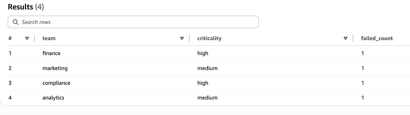
The following screenshot shows aggregated failure counts grouped by team and criticality level.

Viewing data quality results using AWS CLI

Beyond querying results in Athena, you can also retrieve data quality outcomes directly using the AWS Command Line Interface (AWS CLI). This is useful for automation, scripting, and integrating data quality checks into continuous integration and continuous delivery (CI/CD) pipelines.

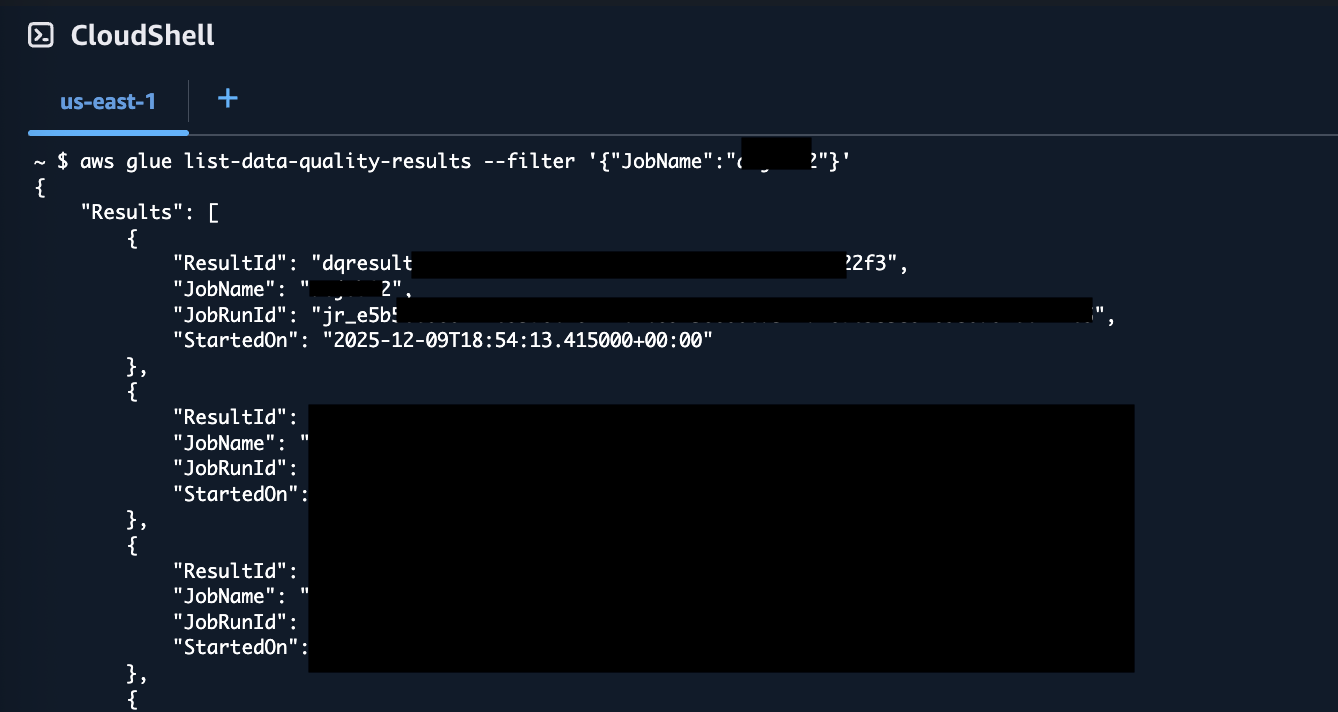
To list data quality results for your ETL job, enter the following:

aws glue list-data-quality-results --filter '{"JobName":"<your-job-name>"}'

You can see in the above screenshot that the resultant JSON includes a ResultId for each data quality run.

To retrieve details of a specific result, enter the following:

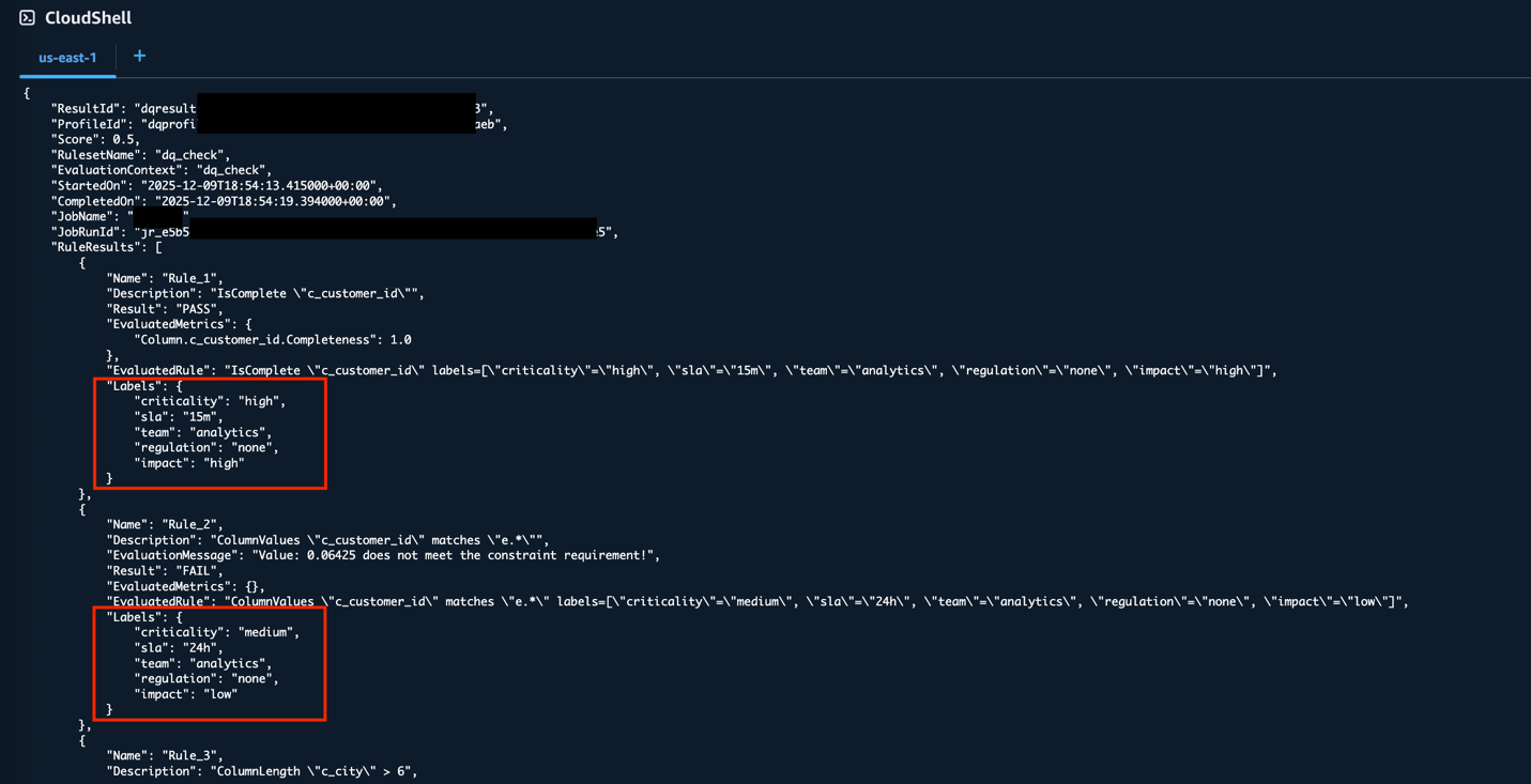
aws glue get-data-quality-result --result-id <result-id>

The output includes a Labels object for each rule in the RuleResults array, containing the label key-value pairs you defined. This provides programmatic access to the same labeled data quality results, which can be useful for automation and scripting workflows.

Cleanup

To avoid incurring ongoing charges, delete the resources created in this post:

  • To delete the S3 folders containing the data quality results, follow the directions at Deleting Amazon S3 objects.
  • To delete the ETL job you created for the test, follow the directions at Delete jobs in the AWS Glue User Guide.
  • To delete the AWS Glue Data Catalog dqrulelevel and dqrowlevel tables, follow the directions at DeleteTable in the AWS Glue Web API Reference.

Conclusion

AWS Glue DQDL labels add organizational context to data quality management by attaching business metadata directly to validation rules. This helps teams identify rule ownership, prioritize failures, and coordinate remediation efforts more effectively.Throughout this post, we’ve seen how AnyCompany moved from managing hundreds of generic rules to implementing a labeled system where data quality results include team ownership and business context. Marketing teams can identify their email validation failures, compliance teams can focus on regulatory violations, and finance teams can address payment-related issues without manual coordination.To implement DQDL Labels in your organization:

  • Start simple – Begin with basic organizational dimensions such as team ownership, criticality levels, and SLA requirements. Expand your labeling approach as needed.
  • Establish standards – Define your label taxonomy up front, including default values for unused dimensions. This consistency supports analytics across teams.
  • Integrate gradually – Add labels to existing rule sets during routine maintenance.
  • Use analytics – Apply the Athena query patterns from this post to build tools such as dashboards and alerting workflows.
  • Build smart automation – Explore creating alerts and notifications tailored to your business criticality and SLA definitions. For example, configure immediate notifications for high-criticality compliance failures while batching low-priority marketing issues into daily reports.

We look forward to seeing how you implement DQDL labels in your organization and expand beyond the examples we’ve covered here. To dive into the AWS Glue Data Quality APIs, refer to Data Quality API documentation. To learn more about AWS Glue Data Quality, check out AWS Glue Data Quality.


About the authors

Arun A K

Arun A K

Arun is a Senior Big Data Specialist Solutions Architect at Amazon Web Services (AWS). He helps customers design and scale data platforms that power innovation through analytics and AI. Arun is passionate about exploring how data and emerging technologies can solve real-world problems. Outside of work, he enjoys sharing knowledge with the tech community and spending time with his family.

Annie Wang

Annie Wang

Annie is a Software Development Engineer at AWS Glue. She focuses on building data quality features, including DQDL, that help customers define, monitor, and validate data quality across their pipelines. She is passionate about making data reliability easier for customers.

Roshin Babu

Roshin Babu

Roshin is a Sr. Specialist Solutions Architect at AWS, where he collaborates with the sales team to support public sector clients. When he’s not working, Roshin is passionate about exploring new destinations, discovering great food, and enjoying soccer both as a player and fan.

Apache Spark 4.0.1 preview now available on Amazon EMR Serverless

Post Syndicated from Al MS original https://aws.amazon.com/blogs/big-data/apache-spark-4-0-1-preview-now-available-on-amazon-emr-serverless/

Amazon EMR Serverless now supports Apache Spark 4.0.1 in preview, making analytics accessible to more users, simplifying data engineering workflows, and strengthening governance capabilities. The release introduces ANSI SQL compliance, VARIANT data types support for JSON handling, Apache Iceberg v3 table format support, and enhanced streaming capabilities. This preview is available in all regions where EMR Serverless is available.

In this post, we explore key benefits, technical capabilities, and considerations for getting started with Spark 4.0.1 on Amazon EMR Serverless—a serverless deployment option that simplifies running open-source big data frameworks, without requiring managing clusters. With the emr-spark-8.0-preview release label, you can evaluate new SQL capabilities, Python API improvements, and streaming enhancements in your existing EMR Serverless environment.

Benefits

Spark 4.0.1 helps you solve data engineering problems with specific improvements. This section shows how new capabilities help with real-world scenarios.

Make analytics accessible to more users

Simplify Extract Transform Load (ETL) development with SQL scripting. Data engineers often switch between SQL and Python to build complex ETL logic with control flow. SQL scripting in Spark 4.0.1 enables loops, conditionals, and session variables directly in SQL, reducing context-switching and simplifying pipeline development. Use pipe syntax (|>) to chain operations for more readable, maintainable queries.

Improve data quality with ANSI SQL mode. Silent type conversion failures can introduce data quality issues. ANSI SQL mode (now default) enforces standard SQL behavior, raising errors for invalid operations instead of producing unexpected results. Important: ANSI SQL mode is now enabled by default. Test your queries thoroughly during this preview evaluation.

Simplify data engineering workflows

Process JSON data efficiently with VARIANT. Teams working with semi-structured data often see slow performance from repeated JSON parsing. The VARIANT data type stores JSON in an optimized binary format, eliminating parsing overhead. You can efficiently store and query JSON data in data lakes without schema rigidity.

Build Python data sources without Scala. Integrating custom data sources previously required Scala expertise. The Python data Source API lets you build connectors entirely in Python, using existing Python skills and libraries without learning a new language.

Debug streaming applications with queryable state. Troubleshooting stateful streaming applications has historically required indirect methods. The new state data source reader shows streaming state as queryable DataFrames. You can inspect state during debugging, test state values in unit tests, and diagnose production incidents.

Strengthen governance capabilities

Establish comprehensive audit trails with Apache Iceberg v3. The Apache Iceberg v3 table format provides transaction guarantees and tracks data changes over time, giving you the audit trails needed for regulatory compliance. When combined with VARIANT data type support, you can maintain governance controls while handling semi-structured data efficiently in data lakes.

Key capabilities

Spark 4.0.1 Preview on EMR Serverless introduces four major capability areas:

  1. SQL enhancements – ANSI mode, pipe syntax, VARIANT type, SQL scripting, user-defined functions (UDFs)
  2. Python API advances – custom data sources, UDF profiling
  3. Streaming improvements – stateful processing API v2, queryable state
  4. Table format support – Amazon S3 Tables, AWS Lake Formation integration

The following sections provide technical details and code examples for each capability.

SQL enhancements

Spark 4.0.1 introduces new SQL capabilities including ANSI mode compliance, SQL UDFs, pipe syntax for readable queries, VARIANT type for JSON handling, and SQL scripting with control flow.

ANSI SQL mode by default

ANSI SQL mode is now enabled by default, enforcing standard SQL behavior for data integrity. Silent casting of out-of-range values now raises errors rather than producing unexpected results. Existing queries may behave differently, particularly around null handling, string casting, and timestamp operations. Use spark.sql.ansi.enabled=false if you need legacy behavior during migration.

SQL pipe syntax

You can now chain SQL operations using the |> operator for improved readability. The following example shows how you can replace nested subqueries with a more maintainable pipeline:

FROM customer
|> LEFT OUTER JOIN orders ON c_custkey = o_custkey
|> AGGREGATE COUNT(o_orderkey) c_count GROUP BY c_custkey
|> AGGREGATE COUNT(*) AS custdist GROUP BY c_count
|> ORDER BY custdist DESC

This replaces nested subqueries, making complex transformations easier to understand and maintain.

VARIANT data type

The VARIANT type handles semi-structured JSON/XML data efficiently without repeated parsing. It uses an optimized binary representation internally while maintaining schema-less flexibility. Previously, JSON expressions required repeated parsing, degrading performance. VARIANT eliminates this overhead. The following snippet shows how to parse JSON into the VARIANT type:

df = spark.sql("SELECT parse_json('{\"name\":\"Alice\",\"age\":30}') as data")

Spark 4.0.1 on EMR Serverless supports Apache Iceberg v3, enabling the VARIANT data type with Iceberg tables. This combination provides efficient storage and querying of semi-structured JSON data in your data lake. Store VARIANT columns in Iceberg tables and use Iceberg’s schema evolution and time travel capabilities alongside Spark’s optimized JSON processing. The following example shows how to create an Iceberg table with a VARIANT column:

CREATE TABLE catalog.db.events (
  event_id BIGINT,
  event_data VARIANT,
  timestamp TIMESTAMP
) USING iceberg;

INSERT INTO catalog.db.events SELECT 1, parse_json('{"user":"alice","action":"login"}'), current_timestamp();

SQL scripting with session variables

Manage state and control flow directly in SQL using session variables, and IF/WHILE/FOR statements. The following example demonstrates a loop that populates a results table:

BEGIN
  DECLARE counter INT = 10;
  WHILE counter > 0 DO
    INSERT INTO results VALUES (counter);
    SET counter = counter - 1;
  END WHILE;
END

This enables complex ETL logic entirely in SQL without switching to Python.

SQL user-defined functions

Define custom functions directly in SQL. Functions can be temporary (session-scoped) or permanent (catalog-stored). The following example shows how to register and use a simple UDF:

CREATE FUNCTION plusOne(x INT) RETURNS INT RETURN x + 1;
SELECT plusOne(5);

Python API advances

This section covers new Python capabilities including custom data sources and UDF profiling tools.

Python data source API

You can now build custom data sources in Python without Scala knowledge. The following example shows how to create a simple data source that returns sample data:

from pyspark.sql.datasource import DataSource, DataSourceReader
from pyspark.sql.types import StructType, StructField, StringType, IntegerType

class SampleDataSource(DataSource):
    def schema(self):
        return StructType([
            StructField("name", StringType()),
            StructField("age", IntegerType())
        ])
    
    def reader(self, schema):
        return SampleReader()

class SampleReader(DataSourceReader):
    def read(self, partition):
        yield ("Alice", 30)
        yield ("Bob", 25)

# Register and use
spark.dataSource.register(SampleDataSource)
spark.read.format("SampleDataSource").load().show()

Unified UDF profiling

Profile Python and Pandas UDFs for performance and memory insights. The following code enables performance profiling:spark.conf.set("spark.sql.pyspark.udf.profiler", "perf") # or "memory"

Structured streaming enhancements

This section covers improvements to stateful stream processing, including queryable state and enhanced state management APIs.

Arbitrary stateful processing API v2

The transformWithState operator provides robust state management with timer and TTL support for automatic cleanup, schema evolution capabilities, and initial state support for pre-populating state from batch DataFrames.

State data source reader

Query streaming state as a DataFrame for debugging and monitoring. Previously, state data was internal to streaming queries. Now you can verify state values in unit tests, diagnose production incidents, detect state corruption, and optimize performance. Note: This feature is experimental. Source options and behavior may change in future releases.

State store improvements

Upgraded changelog checkpointing for RocksDB removes performance bottlenecks. Enhanced checkpoint coordination and improved sorted string table (SST) file reuse management optimizes streaming operations.

Table format support

This section covers support for AWS S3 Tables and full table access (FTA) with AWS Lake Formation.

AWS S3 Tables

Use Spark 4.0.1 with AWS S3 Tables, a storage solution that provides managed Apache Iceberg tables with automatic optimization and maintenance. S3 Tables simplify data lake operations by handling compaction, snapshot management, and metadata cleanup automatically.

Full table access with Lake Formation

FTA is supported for Apache Iceberg, Delta Lake, and Apache Hive tables when using AWS Lake Formation, a managed service that simplifies data access control. FTA provides coarse-grained access control at the table level. Note that fine-grained access control (FGAC) with column-level or row-level permissions is not available in this preview.

Getting started

Follow these steps to create an EMR Serverless application, run sample code to test new features, and provide feedback on the preview.

Prerequisites

Before you begin, confirm you have the following:

Note: EMR Studio Notebooks and SageMaker Unified Studio are not supported during this preview. Use the AWS CLI or AWS SDK to submit jobs.

Step 1: Create your EMR Serverless application

Create or update your application with the emr-spark-8.0-preview release label. The following command creates a new application:

aws emr-serverless create-application --type spark \
  --release-label emr-spark-8.0-preview \
  --region us-east-1 --name spark4-test

Step 2: Test sample code

Run this PySpark job to verify setup and test Spark 4.0.1 features:

from pyspark.sql import SparkSession

spark = SparkSession.builder.appName("Spark 4.0.1 Test").getOrCreate()
print(f"Spark Version: {spark.version}")

# Create sample data
data = [("Alice", 34, "Engineering"), ("Bob", 45, "Sales"),
        ("Charlie", 28, "Engineering"), ("Diana", 52, "Marketing")]
df = spark.createDataFrame(data, ["name", "age", "department"])
df.createOrReplaceTempView("employees")

# Test SQL PIPE syntax
try:
    result = spark.sql("""
        FROM employees
        |> WHERE age > 30
        |> SELECT name, age, department
        |> ORDER BY age DESC
    """)
    result.show()
    print("✓ SQL pipe syntax test passed")
except Exception as e:
    print(f"✗ SQL pipe syntax test failed: {e}")

# Test VARIANT data type
try:
    json_data = spark.sql("""
        SELECT parse_json('{"name":"Alice","skills":["Python","Spark","SQL"]}') as data
    """)
    json_data.show(truncate=False)
    print("✓ VARIANT data type test passed")
except Exception as e:
    print(f"✗ VARIANT data type test failed: {e}")

Submit the job with the following command:

aws emr-serverless start-job-run \
    --application-id <your-application-id> \
    --execution-role-arn <your-execution-role-arn> \
    --job-driver '{
        "sparkSubmit": {
            "entryPoint": "s3://<your-bucket>/spark_4_test.py",
            "sparkSubmitParameters": "--conf spark.executor.cores=4 --conf spark.executor.memory=16g"
        }
    }'

Step 3: Test your workloads

Review the Spark SQL Migration Guide and PySpark Migration Guide, then test production workloads in non-production environments. Focus on queries affected by ANSI SQL mode and benchmark performance.

Step 4: Clean up resources

After testing, delete all resources created during this evaluation to avoid ongoing charges:

# Delete the EMR Serverless application
aws emr-serverless delete-application \
    --application-id spark4-test \
    --region us-east-1
# Remove the test script from S3
aws s3 rm s3://<your-bucket>/spark_4_test.py

Migration considerations

Before evaluating Spark 4.0.1, review the updated runtime requirements and behavioral changes that may affect your existing code.

Runtime requirements

  • Scala: Version 2.13.16 required (2.12 support dropped)
  • Java: JDK 17 or higher required (JDK 8 and 11 support removed)
  • Python: Version 3.9+ required, continued support for 3.11 and newly added 3.12 (3.8 support removed)
  • Pandas: Minimum version 2.0.0 (previously 1.0.5)
  • SparkR: Deprecated; migrate to PySpark

Behavioral changes

With ANSI SQL mode enforcement, you may see different behavior in:

  • Null handling: Stricter null propagation in expressions
  • String casting: Invalid casts now raise errors instead of returning null
  • Map key operations: Duplicate keys now raise errors
  • Timestamp conversions: Overflow returns null instead of wrapped values
  • CREATE TABLE statements: Now respect the spark.sql.sources.defaultconfiguration instead of defaulting to Hive format when USING or STORED AS clauses are omitted

You can control many of these behaviors via legacy configuration flags. Consult the official migration guides for details refer: Spark SQL Migration Guide: 3.5 to 4.0 and PySpark Migration Guide: 3.5 to 4.0.

Preview limitations

The following capabilities are not available in this preview:

  • Fine-grained access control: Fine-grained access control (FGAC) with row-level or column-level filtering is not supported in this preview. Jobs with spark.emr-serverless.lakeformation.enabled=true will fail.
  • Spark Connect: Not supported in this preview. Use standard Spark job submission with the StartJobRun API.
  • Open Table Format limitations: Hudi is not supported in this preview. Delta 4.0.0 does not support Flink connectors (deprecated in Delta 4.0.0). Delta Universal Format is not supported in this preview.
  • Connectors: spark-sql-kinesis, emr-dynamodb, and spark-redshift are unavailable.
  • Interactive applications: Livy and JupyterEnterpriseGateway are not included. Also, SageMaker Unified Studio and EMR Studio are not supported.
  • EMR features: Serverless Storage and Materialized Views are not supported.

This preview lets you evaluate Spark 4.0.1’s core capabilities on EMR Serverless, including SQL enhancements, Python API improvements, and streaming state management. Test your migration path, assess performance improvements, and provide feedback to shape the general availability release.

Conclusion

This post showed you how to get started with the Apache Spark 4.0.1 preview release on Amazon EMR Serverless. You explored how the VARIANT data type works with Iceberg v3 to process JSON data efficiently, how SQL scripting and pipe syntax eliminate context-switching for ETL development, and how queryable streaming state simplifies debugging stateful applications. You also learned about the preview limitations, runtime requirements, and behavioral changes to consider during evaluation.

Test the Spark 4.0.1 preview on EMR Serverless and provide feedback through AWS Support to help shape the general availability release.

To learn more about Apache Spark 4.0.1 features, see the Spark 4.0.1 Release Notes. For EMR Serverless documentation, see the EMR Release Guide.

Resources

Apache Spark Documentation

Amazon EMR Resources


About the authors

Al MS

Al MS

Al is a product manager for Amazon EMR at Amazon Web Services.

Emilie Faracci

Emilie Faracci

Emilie is a Software Development Engineer Amazon Web Services, working on Amazon EMR. She focuses on Spark development and has contributed to open-source Apache Spark v4.0.1.

Karthik Prabhakar

Karthik Prabhakar

Karthik is a Data Processing Engines Architect for Amazon EMR at AWS. He specializes in distributed systems architecture and query optimization, working with customers to solve complex performance challenges in large-scale data processing workloads. His focus spans engine internals, cost optimization strategies, and architectural patterns that enable customers to run petabyte-scale analytics efficiently.

[$] Fedora and GPG 2.5

Post Syndicated from jzb original https://lwn.net/Articles/1055053/

The GNU Privacy Guard (GPG)
project decided to break from the OpenPGP standard for email
encryption in 2023, and instead adopted its own homegrown LibrePGP specification. The GPG 2.4
branch, the last one to adhere to OpenPGP, will be reaching the end of
life in mid-2026. The Fedora project is currently having a discussion
about how that affects the distribution, its users, and what to offer
once 2.4 is no longer receiving updates.

Stenberg: The end of the curl bug-bounty program

Post Syndicated from jzb original https://lwn.net/Articles/1055996/

Curl creator Daniel Stenberg has written a blog
post
explaining why the project is ending its bug-bounty
program, which started in April 2019:

The never-ending slop submissions take a serious mental toll to
manage and sometimes also a long time to debunk. Time and energy that
is completely wasted while also hampering our will to live.

I have also started to get the feeling that a lot of the security
reporters submit reports with a bad faith attitude. These “helpers”
try too hard to twist whatever they find into something horribly bad
and a critical vulnerability, but they rarely actively contribute to
actually improve curl. They can go to extreme efforts to argue and
insist on their specific current finding, but not to write a fix or
work with the team on improving curl long-term etc. I don’t think we
need more of that.

There are these three bad trends combined that makes us take this
step: the mind-numbing AI slop, humans doing worse than ever and the
apparent will to poke holes rather than to help.

Stenberg writes that he still expects “the best and our most
valued security reporters
” to continue informing the project when
security vulnerabilities are discovered. The program will officially
end on January 31, 2026.

AWS Weekly Roundup: Amazon EC2 G7e instances with NVIDIA Blackwell GPUs (January 26, 2026)

Post Syndicated from Micah Walter original https://aws.amazon.com/blogs/aws/aws-weekly-roundup-amazon-ec2-g7e-instances-with-nvidia-blackwell-gpus-january-26-2026/

Hey! It’s my first post for 2026, and I’m writing to you while watching our driveway getting dug out. I hope wherever you are you are safe and warm and your data is still flowing!

Our driveway getting snow plowed

This week brings exciting news for customers running GPU-intensive workloads, with the launch of our newest graphics and AI inference instances powered by NVIDIA’s latest Blackwell architecture. Along with several service enhancements and regional expansions, this week’s updates continue to expand the capabilities available to AWS customers.

Last week’s launches

Amazon EC2 G7e instances are now generally available — The new G7e instances accelerated by NVIDIA RTX PRO 6000 Blackwell Server Edition GPUs deliver up to 2.3 times better inference performance compared to G6e instances. With two times the GPU memory and support for up to 8 GPUs providing 768 GB of total GPU memory, these instances enable running medium-sized models of up to 70B parameters with FP8 precision on a single GPU. G7e instances are ideal for generative AI inference, spatial computing, and scientific computing workloads. Available now in US East (N. Virginia) and US East (Ohio).

Additional updates

I thought these projects, blog posts, and news items were also interesting:

Amazon Corretto January 2026 Quarterly Updates — AWS released quarterly security and critical updates for Amazon Corretto Long-Term Supported (LTS) versions of OpenJDK. Corretto 25.0.2, 21.0.10, 17.0.18, 11.0.30, and 8u482 are now available, ensuring Java developers have access to the latest security patches and performance improvements.

Amazon ECR now supports cross-repository layer sharing — Amazon Elastic Container Registry now enables you to share common image layers across repositories through blob mounting. This feature helps you achieve faster image pushes by reusing existing layers and reduce storage costs by storing common layers once and referencing them across repositories.

Amazon CloudWatch Database Insights expands to four additional regions — CloudWatch Database Insights on-demand analysis is now available in Asia Pacific (New Zealand), Asia Pacific (Taipei), Asia Pacific (Thailand), and Mexico (Central). This feature uses machine learning to help identify performance bottlenecks and provides specific remediation advice.

Amazon Connect adds conditional logic and real-time updates to Step-by-Step Guides — Amazon Connect Step-by-Step Guides now enables managers to build dynamic guided experiences that adapt based on user interactions. Managers can configure conditional user interfaces with dropdown menus that show or hide fields, change default values, or adjust required fields based on prior inputs. The feature also supports automatic data refresh from Connect resources, ensuring agents always work with current information.

Upcoming AWS events

Keep a look out and be sure to sign up for these upcoming events:

Best of AWS re:Invent (January 28-29, Virtual) — Join us for this free virtual event bringing you the most impactful announcements and top sessions from AWS re:Invent. AWS VP and Chief Evangelist Jeff Barr will share highlights during the opening session. Sessions run January 28 at 9:00 AM PT for AMER, and January 29 at 9:00 AM SGT for APJ and 9:00 AM CET for EMEA. Register to access curated technical learning, strategic insights from AWS leaders, and live Q&A with AWS experts.

AWS Community Day Ahmedabad (February 28, 2026, Ahmedabad, India) — The 11th edition of this community-driven AWS conference brings together cloud professionals, developers, architects, and students for expert-led technical sessions, real-world use cases, tech expo booths with live demos, and networking opportunities. This free event includes breakfast, lunch, and exclusive swag.

Join the AWS Builder Center to learn, build, and connect with builders in the AWS community. Browse for upcoming in-person and virtual developer-focused events in your area.


That’s all for this week. Check back next Monday for another Weekly Roundup!

~ micah

Security updates for Monday

Post Syndicated from jzb original https://lwn.net/Articles/1055958/

Security updates have been issued by AlmaLinux (gimp, glib2, go-toolset:rhel8, golang, java-17-openjdk, java-21-openjdk, kernel, net-snmp, pcs, and thunderbird), Debian (apache2, imagemagick, incus, inetutils, libuev, openjdk-17, php7.4, python3.9, shapelib, taglib, and zvbi), Fedora (mingw-glib2, mingw-harfbuzz, mingw-libsoup, mingw-openexr, pgadmin4, python3.11, python3.12, python3.9, and wireshark), Gentoo (Asterisk, Commons-BeanUtils, GIMP, inetutils, and Vim, gVim), Mageia (kernel), Oracle (glib2, java-17-openjdk, java-21-openjdk, and libpng), Red Hat (java-17-openjdk, java-21-openjdk, kernel, and kernel-rt), SUSE (azure-cli-core, bind, buildah, chromium, coredns, glib2, harfbuzz, kernel, kernel-firmware, libheif, libvirt, openCryptoki, openvswitch, podman, python, python-urllib3, rabbitmq-server, and vlang), and Ubuntu (cjson).

Cable cuts, storms, and DNS: a look at Internet disruptions in Q4 2025

Post Syndicated from David Belson original https://blog.cloudflare.com/q4-2025-internet-disruption-summary/

In 2025, we observed over 180 Internet disruptions spurred by a variety of causes – some were brief and partial, while others were complete outages lasting for days. In the fourth quarter, we tracked only a single government-directed Internet shutdown, but multiple cable cuts wreaked havoc on connectivity in several countries. Power outages and extreme weather disrupted Internet services in multiple places, and the ongoing conflict in Ukraine impacted connectivity there as well. As always, a number of the disruptions we observed were due to technical problems – with some acknowledged by the relevant providers, while others had unknown causes. In addition, incidents at several hyperscaler cloud platforms and Cloudflare impacted the availability of websites and applications. 

This post is intended as a summary overview of observed and confirmed disruptions and is not an exhaustive or complete list of issues that have occurred during the quarter. These anomalies are detected through significant deviations from expected traffic patterns observed across our network. Check out the Cloudflare Radar Outage Center for a full list of verified anomalies and confirmed outages. 

Government-directed

Tanzania

The Internet was shut down in Tanzania on October 29 as violent protests took place during the country’s presidential election. Traffic initially fell around 12:30 local time (09:30 UTC), dropping more than 90% lower than the previous week. The disruption lasted approximately 26 hours, with traffic beginning to return around 14:30 local time (11:30 UTC) on October 30. However, that restoration proved to be quite brief, with a significant decrease in traffic occurring around 16:15 local time (13:15 UTC), approximately two hours after it returned. This second near-complete outage lasted until November 3, when traffic aggressively returned after 17:00 local time (14:00 UTC). Nominal drops in announced IPv4 and IPv6 address space were also observed during the shutdown, but there was never a complete loss of announcements, which would have signified a total disconnection of the country from the Internet. (Autonomous systems announce IP address space to other Internet providers, letting them know what blocks of IP addresses they are responsible for.)

Tanzania’s president later expressed sympathy for the members of the diplomatic community and foreigners residing in the country regarding the impact of the Internet shutdown. Internet and social media services were also restricted in 2020 ahead of the country’s general elections.

Cable cuts

Digicel Haiti

Digicel Haiti is unfortunately no stranger to Internet disruptions caused by cable cuts, and the network experienced two more such incidents during the fourth quarter. On October 16, traffic from Digicel Haiti (AS27653) began to fall at 14:30 local time (18:30 UTC), reaching near zero at 16:00 local time (20:00 UTC). A translated X post from the company’s Director General noted: “We advise our clientele that @DigicelHT is experiencing 2 cuts on its international fiber optic infrastructure.” Traffic began to recover after 17:00 local time (21:00 UTC), and reached expected levels within the following hour. At 17:33 local time (21:34 UTC), the Director General posted that “the first fiber on the international infrastructure has been repaired” and service had been restored. 

On November 25, another translated X post from the provider’s Director General stated that its “international optical fiber infrastructure on National Road 1” had been cut. We observed traffic dropping on Digicel’s network approximately an hour earlier, with a complete outage observed between 02:00 – 08:00 local time (07:00 – 13:00 UTC). A follow-on X post at 08:22 local time (13:22 UTC) stated that all services had been restored.

Cybernet/StormFiber (Pakistan)

At 17:30 local time (12:30 UTC) on October 20, Internet traffic for Cybernet/StormFiber (AS9541) dropped sharply, falling to a level approximately 50% the same time a week prior. At the same time, the network’s announced IPv4 address space dropped by over a third. The cause of these shifts was damage to the PEACE submarine cable, which suffered a cut in the Red Sea near Sudan. 

PEACE is one of several submarine cable systems (including IMEWE and SEA-ME-WE-4) that carry international Internet traffic for Pakistani providers. The provider pledged to fully restore service by October 27, but traffic and announced IPv4 address space had recovered to near expected levels by around 02:00 local time on October 21 (21:00 UTC on October 20).

Camtel, MTN Cameroon, Orange Cameroun

Unusual traffic patterns observed across multiple Internet providers in Cameroon on October 23 were reportedly caused by problems on the WACS (West Africa Cable System) submarine cable, which connects countries along the west coast of Africa to Portugal. 

A (translated) published report stated that MTN informed subscribers that “following an incident on the WACS fiber optic cable, Internet service is temporarily disrupted” and Orange Cameroun informed subscribers that “due to an incident on the international access fiber, Internet service is disrupted.” An X post from Camtel stated “Cameroon Telecommunications (CAMTEL) wishes to inform the public that a technical incident involving WACS cable equipment in Batoke (LIMBE) occurred in the early hours of 23 October 2025, causing Internet connectivity disruptions throughout the country.” 

Traffic across the impacted providers originally fell just at around  05:00 local time (04:00 UTC) before recovering to expected levels around 22:00 local time (21:00 UTC). Traffic across these networks was quite volatile during the day, dropping 90-99% at times. It isn’t clear what caused the visible spikiness in the traffic pattern—possibly attempts to shift Internet traffic to other submarine cable systems that connect to Cameroon. Announced IP address space from MTN Cameroon and Orange Cameroon dropped during this period as well, although Camtel’s announced IP address space did not change.

Connectivity in the Central African Republic and Republic of Congo was also reportedly impacted by the WACS issues.

Claro Dominicana

On December 9, we saw traffic from Claro Dominicana (AS6400), an Internet provider in the Dominican Republic, drop sharply around 12:15 local time (16:15 UTC). Traffic levels fell again around 14:15 local time (18:15 UTC), bottoming out 77% lower than the previous week before quickly returning to expected levels. The connectivity disruption was likely caused by two fiber optic outages, as an X post from the provider during the outage noted that they were “causing intermittency and slowness in some services.” A subsequent post on X from Claro stated that technicians had restored Internet services nationwide by repairing the severed fiber optic cables.

Power outages

Dominican Republic

According to a (translated) X post from the Empresa de Transmisión Eléctrica Dominicana (ETED), a transmission line outage caused an interruption in electrical service in the Dominican Republic on November 11. This power outage impacted Internet traffic from the country, resulting in a nearly 50% drop in traffic compared to the prior week, starting at 13:15 local time (17:15 UTC). Traffic levels remained lower until approximately 02:00 local time (06:00 UTC) on December 12, with a later (translated) X post from ETED noting “At 2:20 a.m. we have completed the recovery of the national electrical system, supplying 96% of the demand…”

A subsequent technical report found that “the blackout began at the 138 kV San Pedro de Macorís I substation, where a live line was manually disconnected, triggering a high-intensity short circuit. Protection systems responded immediately, but the fault caused several nearby lines to disconnect, separating 575 MW of generation in the eastern region from the rest of the grid. The imbalance caused major power plants to trip automatically as part of their built-in safety mechanisms.”

Kenya

On December 9, a major power outage impacted multiple regions across Kenya. Kenya Power explained that the outage “was triggered by an incident on the regional Kenya-Uganda interconnected power network, which caused a disturbance on the Kenyan side of the system” and claimed that “[p]ower was restored to most of the affected areas within approximately 30 minutes.” However, impacts to Internet connectivity lasted for nearly four hours, between 19:15 – 23:00 local time (16:15 – 20:00 UTC). The power outage caused traffic to drop as much as 18% at a national level, with the traffic shifts most visible in Nakuru County and Kaimbu County.

Military action

Odesa, Ukraine

Russian drone strikes on the Odesa region in Ukraine on December 12 damaged warehouses and energy infrastructure, with the latter causing power outages in parts of the region. Those outages disrupted Internet connectivity, resulting in traffic dropping by as much as 57% as compared to the prior week. After the initial drop at midnight on December 13 (22:00 UTC on December 12), traffic gradually recovered over the following several days, returning to expected levels around 14:30 local time (12:30 UTC) on December 16.

Weather

Jamaica

Hurricane Melissa made landfall on Jamaica on October 28 and left a trail of damage and destruction in its path. Associated power outages and infrastructure damage impacted Internet connectivity, causing traffic to initially drop by approximately half, starting around 06:15 local time (11:15 UTC), ultimately reaching as much as 70% lower than the previous week. Internet traffic from Jamaica remained well below pre-hurricane levels for several days, and ultimately started to make greater progress towards expected levels during the morning of November 4. It can often take weeks or months for Internet traffic from a country to return to “normal” levels following storms that cause massive and widespread damage – while power may be largely restored within several days, damage to physical infrastructure takes significantly longer to address.

Sri Lanka & Indonesia

On November 26, Cyclone Senyar caused catastrophic floods and landslides in Sri Lanka and Indonesia, killing over 1,000 people and damaging telecommunications and power infrastructure across these countries. The infrastructure damage resulted in disruptions to Internet connectivity, and resultant lower traffic levels, across multiple regions.

In Sri Lanka, regions outside the main Western Province were the most affected, and several provinces saw traffic drop between 80% and 95% as compared to the prior week, including North Western, Southern, Uva, Eastern, Northern, North Central, and Sabaragamuwa.

In Indonesia, Aceh and the Sumatra regions saw the biggest Internet disruptions. In Aceh, traffic initially dropped over 75% as compared to the previous week. In Sumatra, North Sumatra was the most affected, with an early 30% drop as compared to the previous week, before starting to recover more actively the following week.

Known or unspecified technical problems

Smartfren (Indonesia)

On October 3, subscribers to Indonesian Internet provider Smartfren (AS18004) experienced a service disruption. The issues were acknowledged by the provider in an X post, which stated (in translation), “Currently, telephone, SMS and data services are experiencing problems in several areas.” Traffic from the provider fell as much as 84%, starting around 09:00 local time (02:00 UTC). The disruption lasted for approximately eight hours, as traffic returned to expected levels around 17:00 local time (10:00 UTC). Smartfren did not provide any additional information on what caused the service problems.

Vodafone UK

Major British Internet provider Vodafone UK (AS5378 & AS25135) experienced a brief service outage on October 23. At 15:00 local time (14:00 UTC), traffic on both Vodafone ASNs dropped to zero. Announced IPv4 address space from AS5378 fell by 75%, while announced IPv4 address space from AS25135 disappeared entirely. Both Internet traffic and address space recovered two hours later, returning to expected levels around 17:00 local time (16:00 UTC). Vodafone did not provide any information on their social media channels about the cause of the outage, and their network status checker page was also unavailable during the outage.

Fastweb (Italy)

According to a published report, a DNS resolution issue disrupted Internet services for customers of Italian provider Fastweb (AS12874) on October 22, causing observed traffic volumes to drop by over 75%. Fastweb acknowledged the issue, which impacted wired Internet customers between 09:30 – 13:00 local time (08:30 – 12:00 UTC).

Although not an Internet outage caused by connectivity failure, the impact of DNS resolution issues on Internet traffic is very similar. When a provider’s DNS resolver is experiencing problems, switching to a service like Cloudflare’s 1.1.1.1 public DNS resolver will often restore connectivity.

SBIN, MTN Benin, Etisalat Benin

On December 7, a concurrent drop in traffic was observed across SBIN (AS28683), MTN Benin (AS37424), and Etisalat Benin (AS37136). Between 18:30 – 19:30 local time (17:30 – 18:30 UTC), traffic dropped as much as 80% as compared to the prior week at a country level, nearly 100% at Etisalat and MTN, and over 80% at SBIN.

While an attempted coup had taken place earlier in the day, it is unclear whether the observed Internet disruption was related in any way. From a routing perspective, all three impacted networks share Cogent (AS174) as an upstream provider, so a localized issue at Cogent may have contributed to the brief outage.  

Cellcom Israel

According to a reported announcement from Israeli provider Cellcom (AS1680), on December 18, there was “a malfunction affecting Internet connectivity that is impacting some of our customers.” This malfunction dropped traffic nearly 70% as compared to the prior week, and occurred between 09:30 – 11:00 local time (07:30 – 09:00 UTC). The “malfunction” may have been a DNS failure, according to a published report.

Partner Communications (Israel)

Closing out 2025, on December 30, a major technical failure at Israeli provider Partner Communications (AS12400) disrupted mobile, TV, and Internet services across the country. Internet traffic from Partner fell by two-thirds as compared to the previous week between 14:00 – 15:00 local time (12:00 – 13:00 UTC). During the outage, queries to Cloudflare’s 1.1.1.1 public DNS resolver spiked, suggesting that the problem may have been related to Partner’s DNS infrastructure. However, the provider did not publicly confirm what caused the outage.

Cloud Platforms

During the fourth quarter, we launched a new Cloud Observatory page on Radar that tracks availability and performance issues at a region level across hyperscaler cloud platforms, including Amazon Web Services, Microsoft Azure, Google Cloud Platform, and Oracle Cloud Infrastructure.

Amazon Web Services

On October 20, the Amazon Web Services us-east-1 region in Northern Virginia experienced “increased error rates and latencies” that affected multiple services within the region. The issues impacted not only customers with public-facing Web sites and applications that rely on infrastructure within the region, but also Cloudflare customers that have origin resources hosted in us-east-1.

We began to see the impact of the problems around 06:30 UTC, as the share of error (5xx-class) responses began to climb, reaching as high as 17% around 08:00 UTC. The number of failures encountered when attempting to connect to origins in us-east-1 climbed as well, peaking around 12:00 UTC.

The impact could also be clearly seen in key network performance metrics, which remained elevated throughout the incident, returning to normal levels just before the end of the incident, around 23:00 UTC. Both TCP and TLS handshake durations got progressively worse throughout the incident—these metrics measure the amount of time needed for Cloudflare to establish TCP and TLS connections respectively with customer origin servers in us-east-1. In addition, the amount of time elapsed before Cloudflare received response headers from the origin increased significantly during the first several hours of the incident, before gradually returning to expected levels.

Microsoft Azure

On October 29, Microsoft Azure experienced an incident impacting Azure Front Door, its content delivery network service. According to Azure’s report on the incident, “A specific sequence of customer configuration changes, performed across two different control plane build versions, resulted in incompatible customer configuration metadata being generated. These customer configuration changes themselves were valid and non-malicious – however they produced metadata that, when deployed to edge site servers, exposed a latent bug in the data plane. This incompatibility triggered a crash during asynchronous processing within the data plane service.”

The incident report marked the start time at 15:41 UTC, although we observed the volume of failed connection attempts to Azure-hosted origins begin to climb about 45 minutes prior. The TCP and TLS handshake metrics also became more volatile during the incident period, with TCP handshakes taking over 50% longer at times, and TLS handshakes taking nearly 200% longer at peak. The impacted metrics began to improve after 20:00 UTC, and according to Microsoft, the incident ended at 00:05 UTC on October 30.

Cloudflare

In addition to the outages discussed above, Cloudflare also experienced two disruptions during the fourth quarter. While these were not Internet outages in the classic sense, they did prevent users from accessing Web sites and applications delivered and protected by Cloudflare when they occurred.

The first incident took place on November 18, and was caused by a software failure triggered by a change to one of our database systems’ permissions, which caused the database to output multiple entries into a “feature file” used by our Bot Management system. Additional details, including a root cause analysis and timeline, can be found in the associated blog post.

The second incident occurred on December 5, and impacted a subset of customers, accounting for approximately 28% of all HTTP traffic served by Cloudflare. It was triggered by changes being made to our request body parsing logic while attempting to detect and mitigate a newly disclosed industry-wide React Server Components vulnerability. A post-mortem blog post contains additional details, including a root cause analysis and timeline.

For more information about the work underway at Cloudflare to prevent outages like these from happening again, check out our blog post detailing “Code Orange: Fail Small.”

Conclusion

The disruptions observed in the fourth quarter underscore the importance of real-time data in maintaining global connectivity. Whether it’s a government-ordered shutdown or a minor technical issue, transparency allows the technical community to respond faster and more effectively. We will continue to track these shifts on Cloudflare Radar, providing the insights needed to navigate the complexities of modern networking. We share our observations on the Cloudflare Radar Outage Center, via social media, and in posts on blog.cloudflare.com. Follow us on social media at @CloudflareRadar (X), noc.social/@cloudflareradar (Mastodon), and radar.cloudflare.com (Bluesky), or contact us via email.

As a reminder, while these blog posts feature graphs from Radar and the Radar Data Explorer, the underlying data is available from our API. You can use the API to retrieve data to do your own local monitoring or analysis, or you can use the Radar MCP server to incorporate Radar data into your AI tools.

Kernel prepatch 6.19-rc7

Post Syndicated from corbet original https://lwn.net/Articles/1055796/

The 6.19-rc7 kernel prepatch is out for
testing.

So normally this would be the last rc of the release, but as I’ve
mentioned every rc (because I really want people to be aware and be
able to plan for things) this release we’ll have an rc8 due to the
holiday season.

And while some of the early rc’s were smaller than usual and it
didn’t seem necessary, right now I’m quite happy I made that
call. Not because there’s anything particularly scary here – the
release seems to be going fairly smoothly – but because this rc7
really is larger than things normally are and should be at this
point.


Along with the usual fixes, this -rc also includes a new
document
describing the process to replace the kernel project
leadership should that become necessary in the absence of an arranged
transition. The plan largely follows what was decided at the Maintainers Summit in December.

The collective thoughts of the interwebz