Post Syndicated from Oglaf! -- Comics. Often dirty. original https://www.oglaf.com/hook/


Post Syndicated from Oglaf! -- Comics. Often dirty. original https://www.oglaf.com/hook/
Post Syndicated from Cliff Robinson original https://www.servethehome.com/phison-pascari-d205v-122-88tb-nvme-ssd-at-fms-2025/
We saw the Phison Pascari D205V 122.88TB NVMe SSDs at FMS 2025 in both U.2 and E3.L PCIe Gen5 form factors
The post Phison Pascari D205V 122.88TB NVMe SSD at FMS 2025 appeared first on ServeTheHome.
Post Syndicated from Geographics original https://www.youtube.com/watch?v=85bZWxTmdy0
Post Syndicated from Techmoan original https://www.youtube.com/watch?v=PC94KQtNPWs
Post Syndicated from Patrick Kennedy original https://www.servethehome.com/asrock-rack-amponed8-2t-bcm-ampereone-motherboard-at-fms-2025/
The ASRock Rack AMPONED8-2T/BCM is a standard format motherboard that uses the Arm-based Ampere AmpereOne processors along with lots of I/O
The post ASRock Rack AMPONED8-2T BCM AmpereOne Motherboard at FMS 2025 appeared first on ServeTheHome.
Post Syndicated from The History Guy: History Deserves to Be Remembered original https://www.youtube.com/shorts/tBrd62Rl5eo
Post Syndicated from Explosm.net original https://explosm.net/comics/nobody-listens
New Cyanide and Happiness Comic
Post Syndicated from Bruce Schneier original https://www.schneier.com/blog/archives/2025/08/friday-squid-blogging-squid-shaped-ufo-spotted-over-texas.html
Here’s the story. The commenters on X (formerly Twitter) are unimpressed.
As usual, you can also use this squid post to talk about the security stories in the news that I haven’t covered.
Post Syndicated from Pathik Shah original https://aws.amazon.com/blogs/big-data/transform-your-data-to-amazon-s3-tables-with-amazon-athena/
Organizations today manage vast amounts of data, with much of it stored based on initial use cases and business needs. As requirements for this data evolve—whether for real-time reporting, advanced machine learning (ML), or cross-team data sharing—the original storage formats and structures often become a bottleneck. When this happens, data teams frequently find that datasets that worked well for their original purpose now require complex transformations; custom extract, transform, and load (ETL) pipelines; and extensive redesign to unblock new analytical workflows. This creates a significant barrier between valuable data and actionable insights.
Amazon Athena offers a solution through its serverless, SQL-based approach to data transformation. With the CREATE TABLE AS SELECT (CTAS) functionality in Athena, you can transform existing data and create new tables in the process, using standard SQL statements to help reduce the need for custom ETL pipeline development.
This CTAS experience now supports Amazon S3 Tables, which provide built-in optimization, Apache Iceberg support, automatic table maintenance, and ACID transaction capabilities. This combination can help organizations modernize their data infrastructure, achieve improved performance, and reduce operational overhead.
You can use this approach to transform data from commonly used tabular formats, including CSV, TSV, JSON, Avro, Parquet, and ORC. The resulting tables are immediately accessible for querying across Athena, Amazon Redshift, Amazon EMR, and supported third-party applications, including Apache Spark, Trino, DuckDB, and PyIceberg.
This post demonstrates how Athena CTAS simplifies the data transformation process through a practical example: migrating an existing Parquet dataset into S3 Tables.
Consider a global apparel ecommerce retailer processing thousands of daily customer reviews across marketplaces. Their dataset, currently stored in Parquet format in Amazon Simple Storage Service (Amazon S3), requires updates whenever customers modify ratings and review content. The business needs a solution that supports ACID transactions—the ability to atomically insert, update, and delete records while maintaining data consistency—because review data changes frequently as customers edit their feedback.
Additionally, the data team faces operational challenges: manual table maintenance tasks like compaction and metadata management, no built-in support for time travel queries to analyze historical changes, and the need for custom processes to handle concurrent data modifications safely.
These requirements point to a need for an analytics-friendly solution that can handle transactional workloads while providing automated table maintenance, reducing the operational overhead that currently burdens their analysts and engineers.
S3 Tables and Athena provide an ideal solution for these requirements. S3 Tables provide storage optimized for analytics workloads, offering Iceberg support with automatic table maintenance and continuous optimization. Athena is a serverless, interactive query service you can use to analyze data using standard SQL without managing infrastructure. When combined, S3 Tables handle the storage optimization and maintenance automatically, and Athena provides the SQL interface for data transformation and querying. This can help reduce the operational overhead of manual table maintenance while providing efficient data management and optimal performance across supported data processing and query engines.
In the following sections, we show how to use the CTAS functionality in Athena to transform the Parquet-formatted review data into S3 Tables with a single SQL statement. We then demonstrate how to manage dynamic data using INSERT, UPDATE, and DELETE operations, showcasing the ACID transaction capabilities and metadata query features in S3 Tables.
In this walkthrough, we will be working with synthetic customer review data that we’ve made publicly available at s3://aws-bigdata-blog/generated_synthetic_reviews/data/. To follow along, you must have the following prerequisites:
AmazonAthenaFullAccess managed policys3://aws-bigdata-blog/generated_synthetic_reviews/data/You will create an S3 table bucket named athena-ctas-s3table-demo as part of this walkthrough. Make sure this name is available in your chosen AWS Region.
Let’s start by creating a database and source table to hold our Parquet data. This table will serve as the data source for our CTAS operation.
Navigate to the Athena query editor to run the following queries:
Because the data is partitioned by product category, you must add the partition information to the table metadata using MSCK REPAIR TABLE:
The preview query should return sample review data, confirming the table is ready for transformation:
Table buckets are designed to store tabular data and metadata as objects for analytics workloads. Follow these steps to create a table bucket:
athena-ctas-s3table-demo.You can now see athena-ctas-s3table-demo listed under Table buckets.
Namespaces provide logical organization for tables within your S3 table bucket, facilitating scalable table management. In this step, we create a reviews_namespace to organize our customer review tables. Follow these steps to create the table namespace:
athena-ctas-s3table-demo.reviews_namespace for Namespace name.You should now see your S3 Tables configuration automatically selected under Data, as shown in the following screenshot.
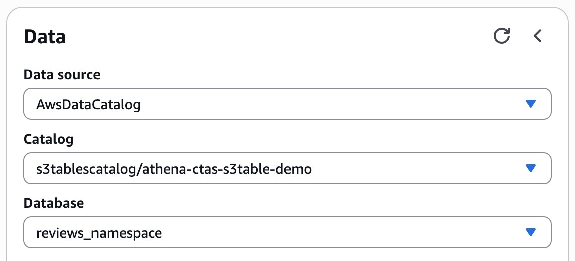
When you enable Integration with AWS analytics services, when creating an S3 table bucket, AWS Glue creates a new catalog called s3tablescatalog in your account’s default Data Catalog specific to your Region. The integration maps the S3 table bucket resources in your account and Region in this catalog.
This configuration makes sure subsequent queries will target your S3 Tables namespace. You’re now ready to create tables using the CTAS functionality.
A table represents a structured dataset consisting of underlying table data and related metadata stored in the Iceberg table format. In the following steps, we transform the customer_reviews table that we created earlier on the Parquet dataset into an S3 table using the Athena CTAS statement. We partition by date using the day() partition transforms from Iceberg.
Run the following CTAS query:
This query creates as S3 table with the following optimizations:
day() transform on review_date for fast queries when filtering on datesYou have successfully transformed your Parquet dataset to S3 Tables using a single CTAS statement.
After you create the table, customer_reviews_s3table will appear under Tables in the Athena console. You can also view the table on the Amazon S3 console by choosing the options menu (three vertical dots) next to the table name and choosing View in S3.
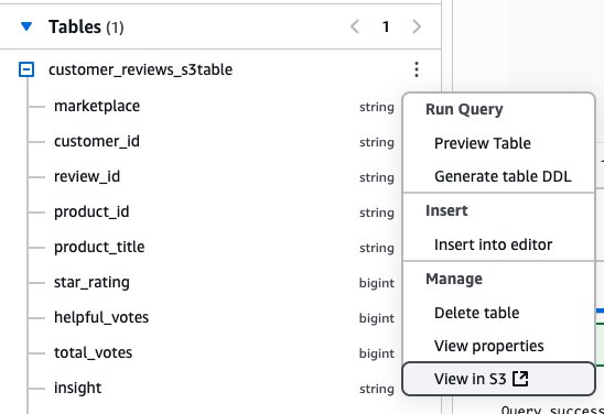
Run a preview query to confirm the data transformation:
Next, let’s analyze monthly review trends:
The following screenshot shows our output.
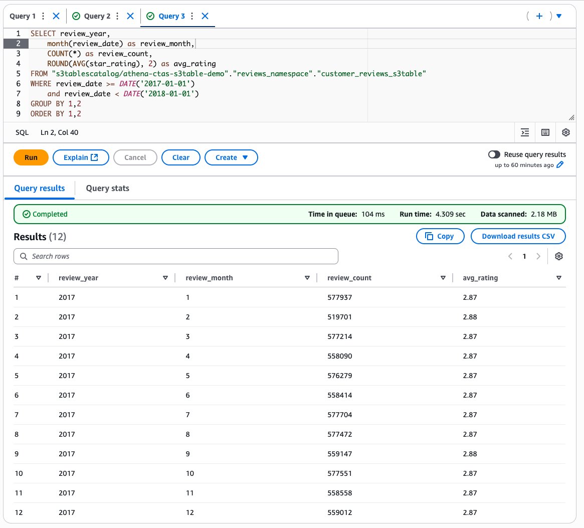
Athena supports standard SQL DML operations (INSERT, UPDATE, DELETE and MERGE INTO) on S3 Tables with full ACID transaction guarantees. Let’s demonstrate these capabilities by adding historical data and performing data quality checks.
Use the following query to insert review data from 2014 and 2015 that wasn’t included in the initial CTAS operation:
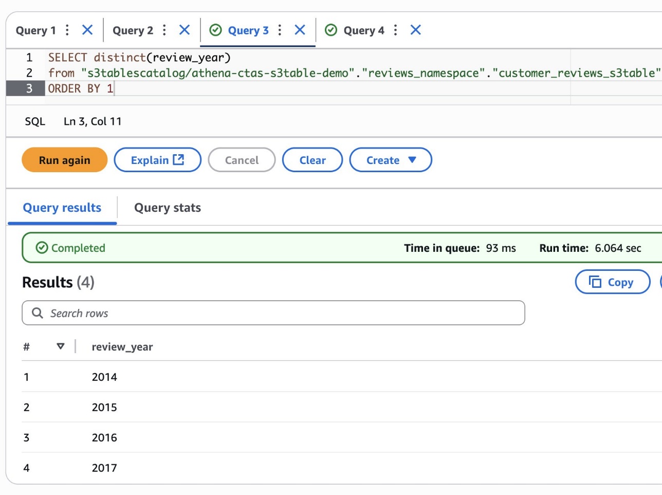
Check which years are now present in the table:
The following screenshot shows our output.
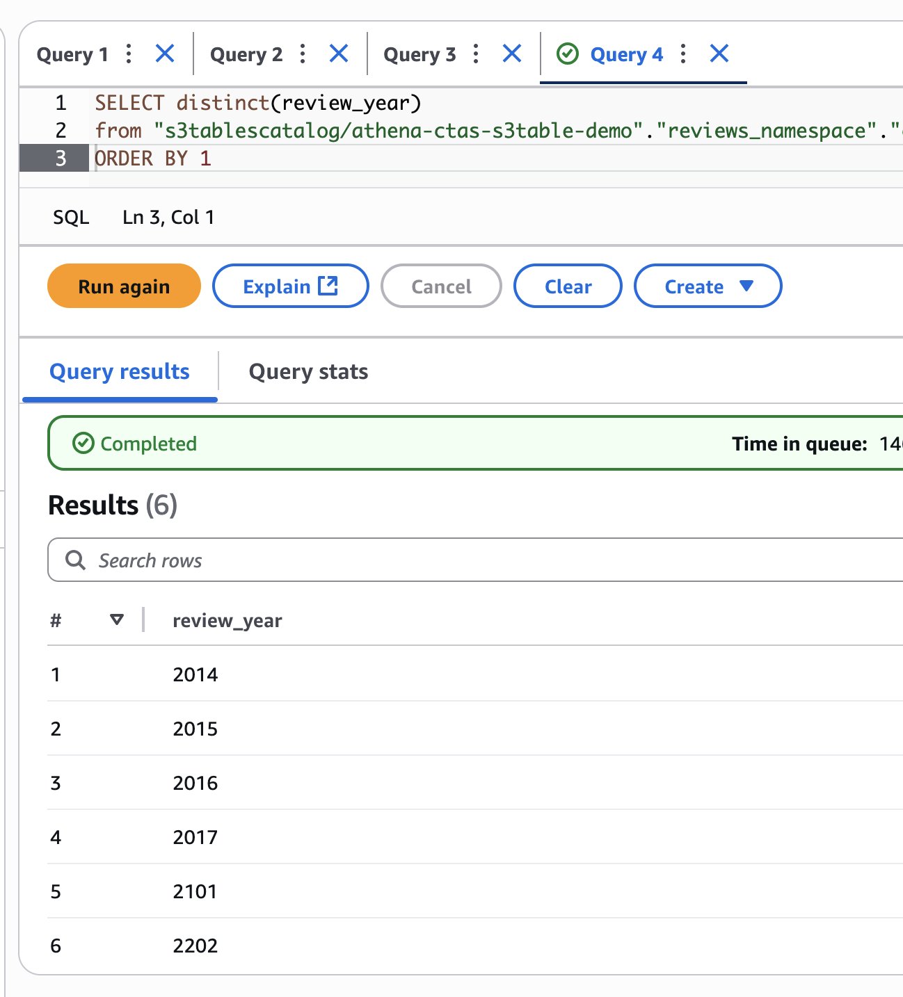
The results show that you have successfully added 2014 and 2015 data. However, you might also notice some invalid years like 2101 and 2202, which appear to be data quality issues in the source dataset.
Remove the records with incorrect years using the S3 Tables DELETE capability:
Confirm the invalid records have been removed.
Let’s demonstrate the UPDATE operation with a business scenario. Imagine the company decides to rebrand the Movies_TV product category to Entertainment_Media to better reflect customer preferences.
First, examine the current product categories and their record counts:
You should see a record with product_category as Movies_TV with approximately 5,690,101 reviews. Use the following query to update all Movies_TV records to the new category name:
Verify the category name change while confirming the record count remains the same:
The results now show Entertainment_Media with the same record count (5,690,101), confirming that the UPDATE operation successfully modified the category name while preserving data integrity.
These examples demonstrate transactional support in S3 Tables through Athena. Combined with automated table maintenance, this helps you build scalable, transactional data lakes more efficiently with minimal operational overhead.
The Athena CTAS functionality supports multiple transformation paths to S3 Tables. The following scenarios demonstrate how organizations can use this capability for various data modernization needs:
These scenarios demonstrate the flexibility of Athena CTAS for various data modernization needs, from simple format conversions to complex data consolidation projects.
To avoid ongoing charges, clean up the resources created during this walkthrough. Complete these steps in the specified order to facilitate proper resource deletion. You might need to add respective delete permissions for databases, table buckets, and tables if your IAM user or role doesn’t already have them.
This post demonstrated how the CTAS functionality in Athena simplifies data transformation to S3 Tables using standard SQL statements. We covered the complete transformation process, including format conversions, ACID operations, and various data transformation scenarios. The solution delivers simplified data transformation through single SQL statements, automatic maintenance, and seamless integration of S3 Tables with AWS analytics services and third-party tools. Organizations can modernize their data infrastructure while achieving enterprise-grade performance.
To get started, begin by identifying datasets that could benefit from optimization or transformation, then refer to Working with Amazon S3 Tables and table buckets and Register S3 table bucket catalogs and query Tables from Athena to implement the transformation patterns demonstrated in this walkthrough. The combination of the serverless capabilities of Athena with the automatic optimizations in S3 Tables can provide a powerful foundation for modern data analytics.
 Pathik Shah is a Sr. Analytics Architect on Amazon Athena. He joined AWS in 2015 and has been focusing in the big data analytics space since then, helping customers build scalable and robust solutions using AWS Analytics services.
 Aritra Gupta is a Senior Technical Product Manager on the Amazon S3 team at Amazon Web Services. He helps customers build and scale data lakes. Based in Seattle, he likes to play chess and badminton in his spare time.
Post Syndicated from jzb original https://lwn.net/Articles/1033954/
Mitchell Hashimoto has written a blog
post about “fully embracing the GObject type system
” with a
rewrite of the GTK version of Ghostty:
In addition to memory management [improvements], we can now more
easily create custom GTK widgets. This let us fully embrace modern GTK
UI technologies such as Blueprint. For example, here is our terminal
window Blueprint file. This has already led to more easily introducing
GUI features like a new GTK titlebar tabs option, an animated border
on bell, etc.
The rewrite is now the default if one builds Ghostty from source,
and will be included in the 1.2 release that is expected in the next
few weeks. LWN covered
Ghostty in January.
Post Syndicated from Explosm.net original https://explosm.net/comics/ziiiiiiiiip
New Cyanide and Happiness Comic
Post Syndicated from Crosstalk Solutions original https://www.youtube.com/watch?v=E1pFWyIzPsE
Post Syndicated from Channy Yun (윤석찬) original https://aws.amazon.com/blogs/aws/aws-named-as-a-leader-in-2025-gartner-magic-quadrant-for-strategic-cloud-platform-services-for-15-years-in-a-row/
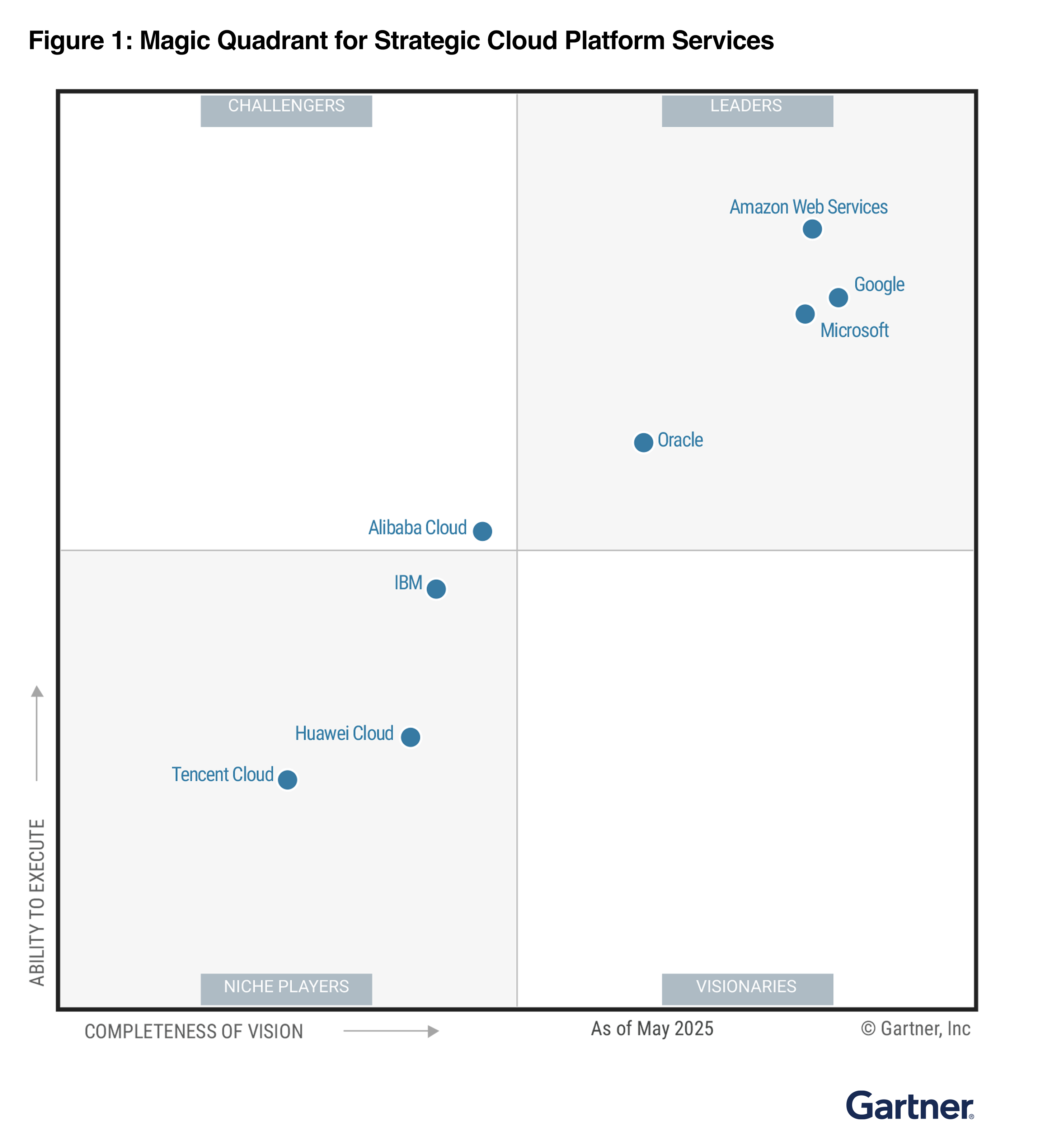
On August 4, 2025, Gartner published its Gartner Magic Quadrant for Strategic Cloud Platform Services (SCPS). Amazon Web Services (AWS) is the longest-running Magic Quadrant Leader, with Gartner naming AWS a Leader for the fifteenth consecutive year.
In the report, Gartner once again placed AWS highest on the “Ability to Execute” axis. We believe this reflects our ongoing commitment to giving customers the broadest and deepest set of capabilities to accelerate innovation as well as unparalleled security, reliability, and performance they can trust for their most critical applications.
Here is the graphical representation of the 2025 Magic Quadrant for Strategic Cloud Platform Services.
Gartner recognized AWS strengths as:
The most common feedback I hear from customers is that AWS has the largest and most dynamic cloud community, making it easy to ask questions and learn from millions of active customers and tens of thousands of partners globally. We recently launched our community hub, AWS Builder Center to connect directly with AWS Heroes and AWS Community Builders. You can also explore and join AWS User Groups and AWS Cloud Clubs in a city near you.
We have also focused on facilitating the digital transformation of enterprise customers through a number of enterprise programs, such as the AWS Migration Acceleration Program. Using generative AI on migration and modernization, we introduced AWS Transform, the first agentic AI service developed to accelerate enterprise modernization of mission-critical business workloads such as .NET, mainframe, and VMware.
Access the complete full Gartner report to learn more. It outlines the methodology and evaluation criteria used to develop their assessments of each cloud service provider included in the report. This report can serve as a guide when choosing a cloud provider that helps you innovate on behalf of your customers.
— Channy
Gartner does not endorse any vendor, product or service depicted in its research publications and does not advise technology users to select only those vendors with the highest ratings or other designation. Gartner research publications consist of the opinions of Gartner’s research organization and should not be construed as statements of fact. Gartner disclaims all warranties, expressed or implied, with respect to this research, including any warranties of merchantability or fitness for a particular purpose.
GARTNER is a registered trademark and service mark of Gartner and Magic Quadrant is a registered trademark of Gartner, Inc. and/or its affiliates in the U.S. and internationally and are used herein with permission. All rights reserved.
Post Syndicated from LastWeekTonight original https://www.youtube.com/shorts/VPtAWwRBHUc
Post Syndicated from Sébastien Stormacq original https://aws.amazon.com/blogs/aws/celebrating-10-years-of-amazon-aurora-innovation/
Ten years ago, we announced the general availability of Amazon Aurora, a database that combined the speed and availability of high-end commercial databases with the simplicity and cost-effectiveness of open source databases.
As Jeff described it in its launch blog post: “With storage replicated both within and across three Availability Zones, along with an update model driven by quorum writes, Amazon Aurora is designed to deliver high performance and 99.99% availability while easily and efficiently scaling to up to 64 TiB of storage.”
When we started developing Aurora over a decade ago, we made a fundamental architectural decision that would change the database landscape forever: we decoupled storage from compute. This novel approach enabled Aurora to deliver the performance and availability of commercial databases at one-tenth the cost.
This is one of the reasons why hundreds of thousands of AWS customers choose Aurora as their relational database.
Today, I’m excited to invite you to join us for a livestream event on August 21, 2025, to celebrate a decade of Aurora database innovation.
A brief look back at the past
Throughout the evolution of Aurora, we’ve focused on four core innovation themes: security as our top priority, scalability to meet growing workloads, predictable pricing for better cost management, and multi-Region capabilities for global applications. Let me walk you through some key milestones in the Aurora journey.
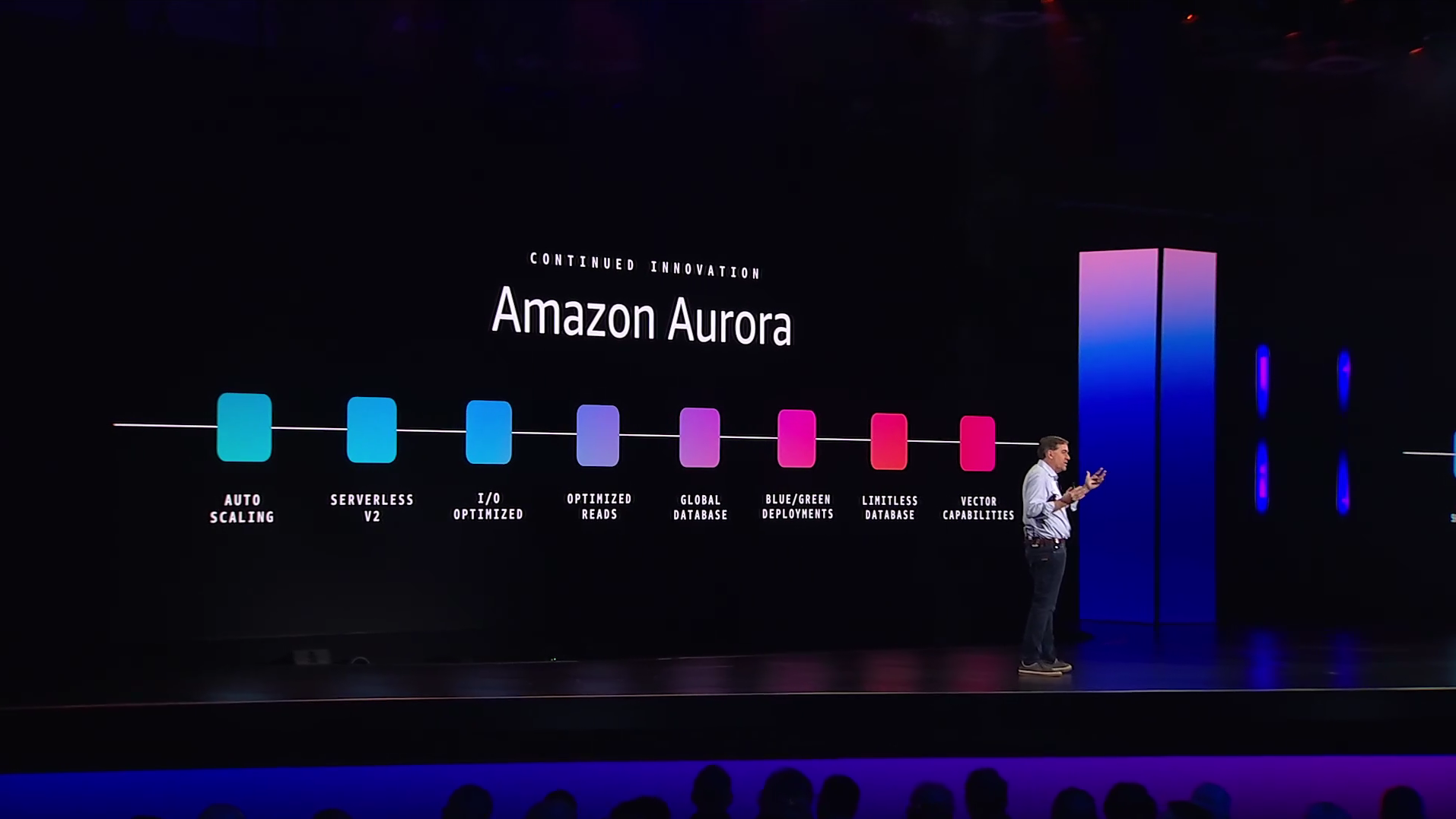
We previewed Aurora at re:Invent 2014, and made it generally available in July 2015. At launch, we presented Aurora as “a new cost-effective MySQL-compatible database engine.”
In June 2016, we introduced reader endpoints and cross-Region read replicas, followed by AWS Lambda integration and the ability to load tables directly from Amazon S3 in October. We added database cloning and export to Amazon S3 capabilities in June 2017 and full compatibility with PostgreSQL in October that year.
The journey continued with the serverless preview in November 2017, which became generally available in August 2018. Global Database launched in November 2018 for cross-Region disaster recovery. We introduced blue/green deployments to simplify database updates, and optimized read instances to improve query performance.
In 2023, we added vector capabilities with pgvector for similarity search for Aurora PostgreSQL, and Aurora I/O-Optimized to provide predictable pricing with up to 40 percent cost savings for I/O-intensive applications. We launched Aurora zero-ETL integration with Amazon Redshift which enables near real-time analytics and ML using Amazon Redshift on petabytes of transactional data from Aurora by removing the need for you to build and maintain complex data pipelines that perform extract, transform, and load (ETL) operations. This year we added Aurora MySQL zero-ETL integration with Amazon Sagemaker, enabling near real-time access of your data in the lakehouse architecture of SageMaker to run a broad range of analytics.
In 2024, we made it as effortless as just one click to select Aurora PostgreSQL as a vector store for Amazon Bedrock Knowledge Bases and launched Aurora PostgreSQL Limitless Database, a serverless horizontal scaling (sharding) capability.
To simplify scaling for customers, we also increased the maximum storage to 128 TiB in September 2020, allowing many applications to operate within a single instance. Last month, we’ve further simplified scaling by doubling the maximum storage to 256 TiB, with no upfront provisioning required and pay-as-you-go pricing based on actual storage used. This enables even more customers to run their growing workloads without the complexity of managing multiple instances while maintaining cost efficiency.
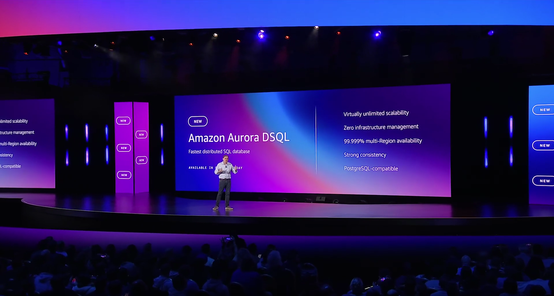
Most recently, at re:Invent 2024, we announced Amazon Aurora DSQL, which became generally available in May 2025. Aurora DSQL represents our latest innovation in distributed SQL databases, offering active-active high availability and multi-Region strong consistency. It’s the fastest serverless distributed SQL database for always available applications, effortlessly scaling to meet any workload demand with zero infrastructure management.
Aurora DSQL builds on our original architectural principles of separation of storage and compute, taking them further with independent scaling of reads, writes, compute, and storage. It provides 99.99% single-Region and 99.999% multi-Region availability, with strong consistency across all Regional endpoints.
And in June, we launched Model Context Protocol (MCP) servers for Aurora, so you can integrate your AI agents with your data sources and services.
Let’s celebrate 10 years of innovation
 By attending the August 21 livestream event, you’ll hear from Aurora technical leaders and founders, including Swami Sivasubramanian, Ganapathy (G2) Krishnamoorthy, Yan Leshinsky, Grant McAlister, and Raman Mittal. You’ll learn directly from the architects who pioneered the separation of compute and storage in cloud databases, with technical insights into Aurora architecture and scaling capabilities. You’ll also get a glimpse into the future of database technology as Aurora engineers share their vision and discuss the complex challenges they’re working to solve on behalf of customers.
The event also offers practical demonstrations that show you how to implement key features. You’ll see how to build AI-powered applications using pgvector, understand cost optimization with the new Aurora DSQL pricing model, and learn how to achieve multi-Region strong consistency for global applications.
The interactive format includes Q&A opportunities with Aurora experts, so you’ll be able to get your specific technical questions answered. You can also receive AWS credits to test new Aurora capabilities.
If you’re interested in agentic AI, you’ll particularly benefit from the sessions on MCP servers, Strands Agents, and how to integrate Strands Agents with Aurora DSQL, which demonstrate how to safely integrate AI capabilities with your Aurora databases while maintaining control over database access.
Whether you’re running mission-critical workloads or building new applications, these sessions will help you understand how to use the latest Aurora features.
Register today to secure your spot and be part of this celebration of database innovation.
To the next decade of Aurora innovation!
Post Syndicated from Matt Granger original https://www.youtube.com/watch?v=T-0P7VBxSrM
Post Syndicated from Jaydev Nath original https://aws.amazon.com/blogs/big-data/export-jmx-metrics-from-kafka-connectors-in-amazon-managed-streaming-for-apache-kafka-connect-with-a-custom-plugin/
Organizations use streaming applications to process and analyze data in real time and adopt the Amazon MSK Connect feature of Amazon Managed Streaming for Apache Kafka (Amazon MSK) to run fully managed Kafka Connect workloads on AWS. Message brokers like Apache Kafka allow applications to handle large volumes and diverse types of data efficiently and enable timely decision-making and instant insights. It’s crucial to monitor the performance and health of each component to help ensure the seamless operation of data streaming pipelines.
Amazon MSK is a fully managed service that simplifies the deployment and operation of Apache Kafka clusters on AWS. It simplifies building and running applications that use Apache Kafka to process streaming data. Amazon MSK Connect simplifies the deployment, monitoring, and automatic scaling of connectors that transfer data between Apache Kafka clusters and external systems such as databases, file systems, and search indices. Amazon MSK Connect is fully compatible with Kafka Connect and supports Amazon MSK, Apache Kafka, and Apache Kafka compatible clusters. Amazon MSK Connect uses a custom plugin as the container for connector implementation logic.
Custom MSK connect plugins use Java Management Extensions (JMX) to expose runtime metrics. While Amazon MSK Connect sends a set of connect metrics to Amazon CloudWatch, it currently does not support exporting the JMX metrics emitted by the connector plugins natively. These metrics can be exported by modifying the custom connect plugin code directly, but it requires maintenance overhead because the plugin code needs to be modified every time it’s updated. In this post, we demonstrate an optimal approach by extending a custom connect plugin with additional modules to export JMX metrics and publish them to CloudWatch as custom metrics. These additional JMX metrics emitted by the custom connectors provide rich insights into their performance and health of the connectors. In this post, we demonstrate how you can export the JMX metrics for Debezium connector when used with MSK Connect.
Before we dive deep into exporting JMX metrics, let’s understand how JMX works. JMX is a technology that you can use to monitor and manage Java applications. Key components involved in JMX monitoring are:
JMX monitoring involves the steps shown in the following figure:

JMX monitoring steps include:
This method of wrapping supported Kafka connectors with custom code that exposes connector-specific operational metrics enables teams to get better insights by correlating various connector metrics with cloud-centered metrics in monitoring systems such as Amazon CloudWatch. This approach enables consistent monitoring across different components of the change data capture (CDC) pipeline, ultimately feeding metrics into unified dashboards while respecting each connector’s architectural philosophy. The consolidated metrics can be delivered to CloudWatch or the monitoring tool of your choice including partner specific application performance management (APM) tools such as Datadog, New Relic, and so on.
We have the working implementation of this same approach with two popular connectors: Debezium source connector and MongoDB Sink Connector. You can find the Github sample and ready to use plugins built for each in the repository. Review the README file for this custom implementation for more details.
For example, our custom implementation for the MongoDB Sink Connector adds a metrics export layer that calculates critical performance indicators such as latest-kafka-time-difference-ms – which measures the latency between Kafka message timestamps and connector processing time by subtracting the connector’s current clock time from the last received record’s timestamp. This custom wrapper around the MongoDB Sink Connector enables exporting relevant JMX metrics and publishing them as custom metrics to CloudWatch. We’ve open sourced this solution on GitHub, along with a ready-to-use plugin and detailed configuration guidance in the README.
CDC is the process of identifying and capturing changes made in a database and delivering those changes in real time to a downstream system. Debezium is an open source distributed platform built on top of Apache Kafka that provides CDC functionality. It provides a set of connectors to track and stream changes from databases to Kafka.
In the next section, we dive deep into the implementation details of how to export JMX metrics from Debezium MySQL Connector deployed as a custom plugin in Amazon MSK Connect. The connector plugin takes care of creating and configuring the MBeans and registering them with the JMX registry.
The following diagram shows the workflow of using Debezium MySQL Connector as a custom plugin in Amazon MSK Connect for CDC from an Amazon Aurora MySQL-Compatible Edition data source.
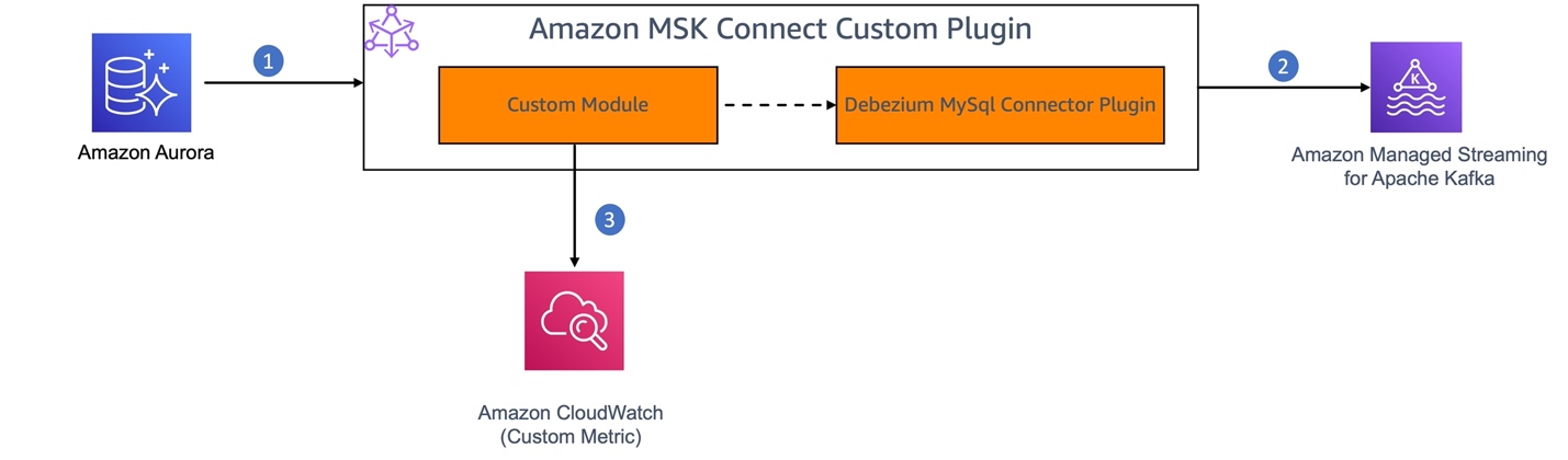
The Debezium connector provides three types of metrics in addition to the built-in support for default Kafka and Kafka Connect JMX metrics.
In this solution, we export the MilliSecondsBehindSource streaming metrics emitted by the Debezium MySQL connector. This metric provides the number of milliseconds that the connector is lagging behind the change events in the database.
Following are the prerequisites you need:
Creating a custom plugin for Amazon MSK Connect for the solution involves the following steps:
This custom module extends the connector functionality to export the JMX metrics without requiring any changes in the underlying connector implementation. This helps ensure that upgrading the custom plugin requires only upgrading the plugin version in the pom.xml of the custom module.
Let’s deep dive and understand the implementation of each step mentioned above.
Create a new Maven project with dependencies on Debezium MySQL Connector to enable JMX monitoring, Kafka Connect API for configuration, and CloudWatch AWS SDK to push the metrics to CloudWatch.
Set up a JMX connector server to enable JMX monitoring: To enable JMX monitoring, the JMX server needs to be started at the time of initializing the connector. This is usually done by setting the environment variables with JMX options as described in Monitoring Debezium. In the case of an Amazon MSK Connect custom plugin, JMX monitoring is enabled programmatically at the time of connector plugin initialization. To achieve this:
MySqlConnector class and override the start which is the connector’s entry point to execute custom code.start method of the custom connector class (DebeziumMySqlMetricsConnector) that we are creating, set the following parameters to allow customization of the JMX Server properties by retrieving connector configuration from a config file.connect.jmx.port – The port number on which the RMI registry needs to be created. JMXConnectorServer would listen to the incoming connections on this port.
database.server.name – Name of the database that is the source for the CDC.
It also retrieves the CloudWatch configuration related properties that will be used while pushing the JMX metrics to CloudWatch.
cloudwatch.namespace.name – CloudWatch NameSpace to which the metrics need to be pushed as custom metrics
cloudwatch.region – CloudWatch Region where the custom namespace is created in your AWS account
connectJMXPort). This registry is used by the JMXConnectorServer to store the RMI objects corresponding to the MBeans in the JMX registry. This allows the JMX clients to look up and access the MBeans on the PlatformMBeanServer.LocateRegistry.createRegistry(connectJMXPort);
PlatformMBeanServer and construct the JMXServiceURL which is in the format service:jmx:rmi://localhost/jndi/rmi://localhost:<<jmx.port>>/jmxrmi. Create a new JMXConnectorServer instance using the JMXConnectorServerFactory and the JMXServiceURL and start the JMXConnectorServer instance.Implement JMX metrics exporter: Create a JMX client to connect to the JMX server, query the MilliSecondBehindSource metric from the JMX server, convert it into the required format, and export it to CloudWatch.
JMXConnectorFactory and JMXServiceURLMilliSecondsBehindSource, and retrieve the metric value using sample code provided in msk-connect-custom-plugin-jmx. (you can choose one or more metrics).getScheduler().schedule(new JMXMetricsExporter(), SCHEDULER_INITIAL_DELAY, SCHEDULER_PERIOD);
Export metrics to CloudWatch: Implement the logic to push relevant JMX metrics to CloudWatch. You can use the AWS SDK for Java to interact with the CloudWatch PutMetricData API or use the CloudWatch Logs subscription filter to ingest the metrics from a dedicated Kafka topic.
For more information, see the sample implementation for the custom module in aws-samples in GitHub. This sample also provides custom plugins packaged with two different versions of Debezium MySQL connector (debezium-connector-mysql-2.5.2.Final-plugin and debezium-connector-mysql-2.7.3.Final-plugin) and the following steps would explain the steps to build a custom plugin using your custom code.
Build and package the Maven project with the custom code as a JAR file and include the JAR file in the debezium-connector-mysql-2.5.2.Final-plugin folder downloaded from maven repo. Package the updated debezium-connector-mysql-2.5.2.Final-plugin as a ZIP file (Amazon MSK Connect accepts custom plugins in ZIP or JAR format). Alternatively, you can use the prebuiltcustom-debezium-mysql-connector-plugin.zip available in GitHub.
Choose the Debezium connector version (2.5 or 2.7) that fits your requirement.
When you have to upgrade to a new version of the Debezium MySQL connector, you can update the version of the dependency and build the custom module and deploy it. By doing this, you can maintain the custom plugin without modifying the original connector code. The GitHub samples provide ready-to-use plugins for two Debezium connector versions. However, you can follow the same approach to upgrade to the latest connector version as well.
msk-lab-${ACCOUNT_ID}-plugins-bucket/debezium .custom-debezium-mysql-connector-plugin.zip to msk-lab-${ACCOUNT_ID}-plugins-bucket/debezium, as shown in the following figure.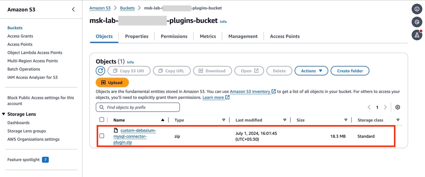
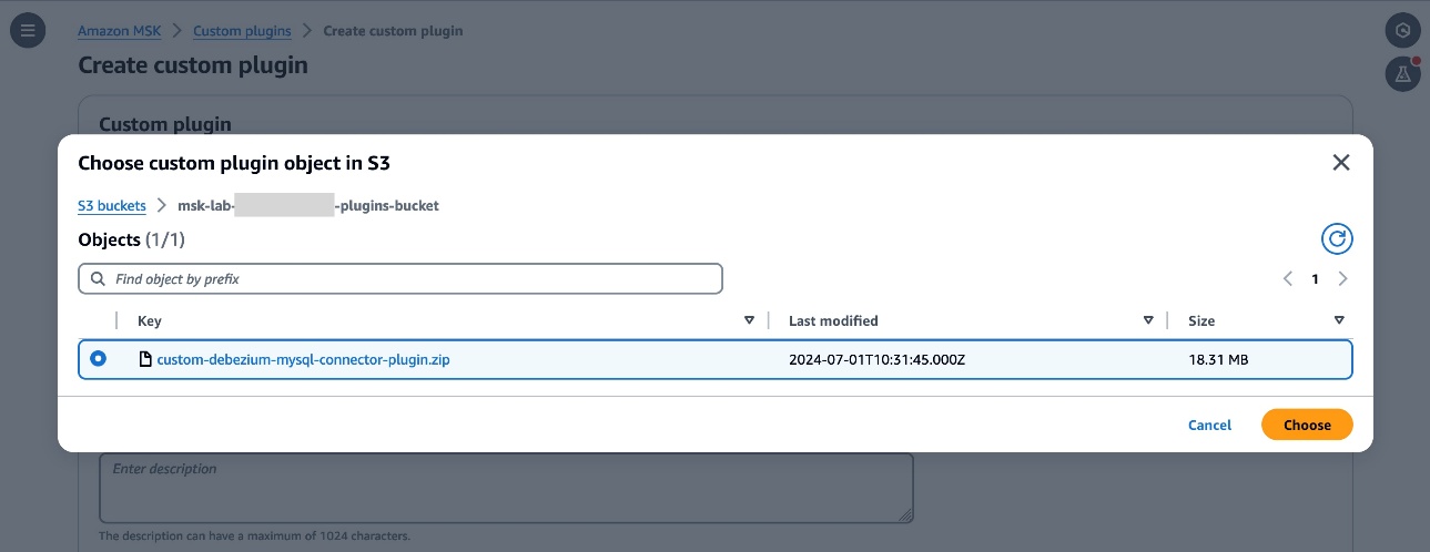
custom-debezium-mysql-connector-plugin for the plugin name. Optionally, enter a description and choose Create Custom Plugin.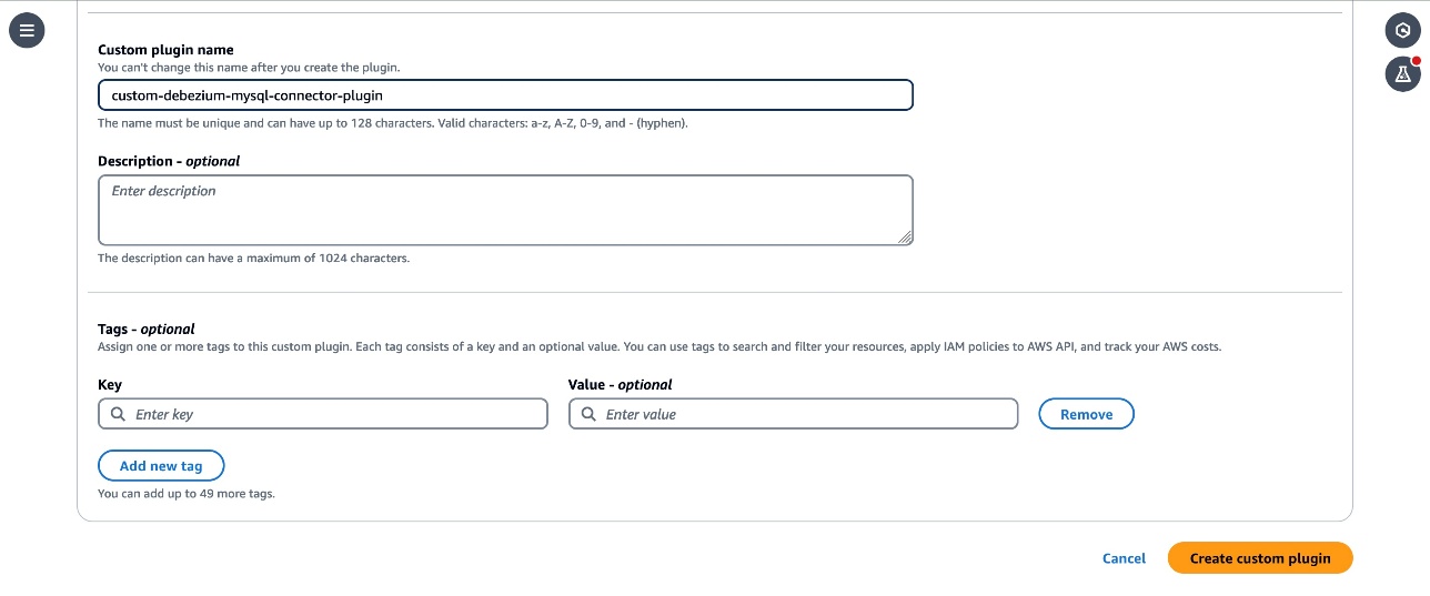
Active.The next step is to create an MSK connector.
custom-debezium-mysql-connector-plugin from the list of Custom plugins, then choose Next.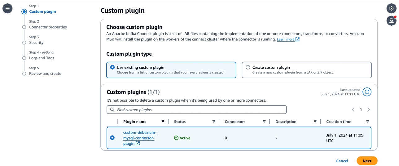
custom-debezium-mysql-connector in the Name textbox, and a description for the connector.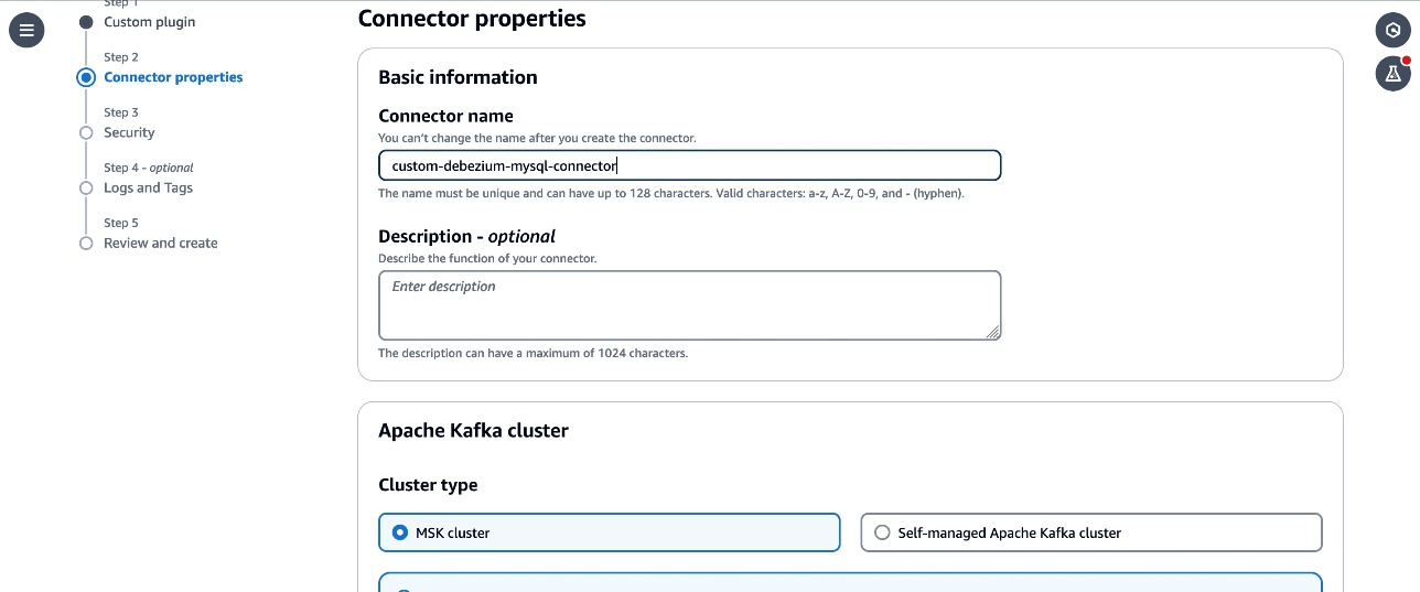
MSKCluster-msk-connect-lab from the listed MSK clusters. From the Authentication dropdown, select IAM.<Your Aurora MySQL database endpoint>, <Your Database Password>, <Your MSK Bootstrap Server Address>, and <Your CloudWatch Region>placeholders with the corresponding details for the resources in your account.topic.prefix, database.user, topic.prefix, database.server.id, database.server.name, database.port, database.include.listparameters in the configuration. These parameters are configured with the values used in the workshop. Update them with the details corresponding to your configuration if you have customized it in your account.connector.classparameter is updated with the qualified name of the subclass of MySqlConnector class that you created in the custom module.connect.jmx.portparameter specifies the default port to start the JMX server. You can configure this to any available port.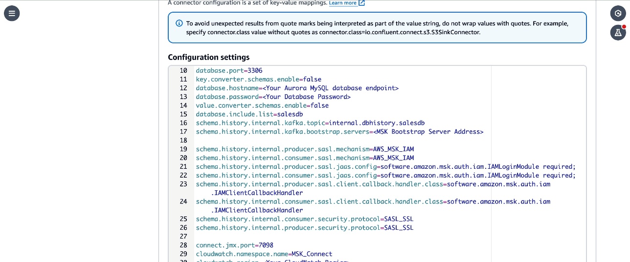
5. Follow the remaining instructions from the Create MSK Connector lab and create the connector. Verify that the connector status changes to Running.
Debezium MySQL custom connector version (2.7.3) provides additional flexibility to configure optional properties that can be added to your MSK connector configuration and selectively include and exclude metrics to emit to CloudWatch. The following are the example configuration properties that can be used with version 2.7.3 :
The following is a sample configuration excerpt.
Review the GitHub README file for more details on the use of these properties with MSK connector configurations.
Follow the instructions in the Verify the replication in the Kafka cluster lab to set up a client and make changes to the source DB and verify that the changes are captured and sent to Kafka topics by the connector.
To verify that the connector has published the JMX metrics to CloudWatch, go to the CloudWatch console and choose Metrics in the navigation pane, then choose All Metrics. Under Custom namespace, you can see MSK_Connect with database name as the dimension. Select the database name to view the metrics.
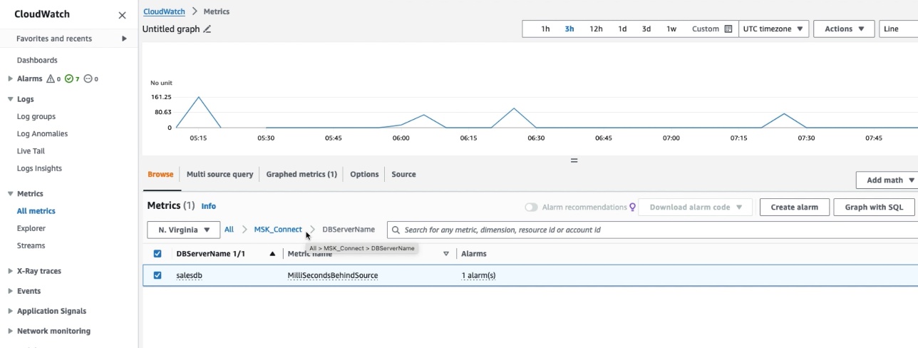
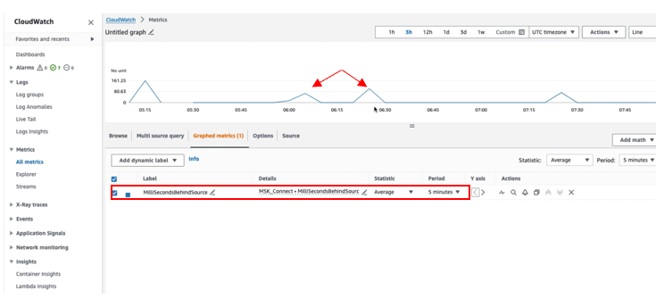
Select the MilliSecondBehindSource metric with statistic as Average in the Graphed Metric to plot the graph. You can verify that the MilliSecondBehindSource metric value is greater than zero whenever any operation is being performed on the source database and returns to zero during the idle time.
Delete the resources that you created such as the Aurora DB, Amazon MSK Cluster and connectors by following the instructions at Cleanup in the Amazon MSK Connect lab if you have been following along to set up the solution on your account.
In this post, we showed you how to extend the Debezium MySQL connector plugin with an additional module to export the JMX metrics to CloudWatch as custom metrics. As a next step, you can create a CloudWatch alarm to monitor the metrics and take remediation actions when the alarm is triggered. In addition to exporting the JMX metrics to CloudWatch, you can export these metrics to third-party applications such as Prometheus or DataDog using CloudWatch Metric Streams. You can follow a similar approach to export the JMX metrics of other connectors from MSK Connect. You can learn more about creating your own connectors by visiting the Connector Developer Guide and how to deploy them as custom plugins in the MSK Connect documentation.
 Jaydev Nath is a Solutions Architect at AWS, where he works with ISV customers to build secure, scalable, reliable, and cost-efficient cloud solutions. He brings strong expertise in building SaaS architecture on AWS with a focus on Generative AI and data analytics technologies to help deliver practical, valuable business outcomes for customers.
 David John Chakram is a Principal Solutions Architect at AWS. He specializes in building data platforms and architecting seamless data ecosystems. With a profound passion for databases, data analytics, and machine learning, he excels at transforming complex data challenges into innovative solutions and driving businesses forward with data-driven insights.
 Sharmila Shanmugam is a Solutions Architect at Amazon Web Services. She is passionate about solving the customers’ business challenges with technology and automation and reduce the operational overhead. In her current role, she helps customers across industries in their digital transformation journey and build secure, scalable, performant and optimized workloads on AWS.
Post Syndicated from jzb original https://lwn.net/Articles/1032947/
The purpose of the Filesystem
Hierarchy Standard (FHS) is to provide a specification for
filesystem layout; it specifies the location for files and directories
on a Linux system to simplify application development for multiple
distributions. In its heyday it had some success at this, but the
standard has been frozen in time since 2015, and much has changed
since then. There is a slow-moving effort
to revive the FHS and create a FHS 4.0, but a recent discussion
among Fedora developers also raised the possibility of standardizing
on the suggestions in systemd’s file-hierarchy
documentation, which has now been added to the Linux Userspace API
(UAPI) Group’s specifications.
Post Syndicated from daroc original https://lwn.net/Articles/1033901/
Security updates have been issued by AlmaLinux (kernel and webkit2gtk3), Debian (aide and postgresql-13), Fedora (libtiff, mupdf, and pandoc), SUSE (cairo, chromium, gstreamer-plugins-base, ImageMagick, iputils, kubernetes1.23, kubernetes1.26, matrix-synapse, Mesa, pgadmin4, python3, qemu, and rz-pm), and Ubuntu (aide).