Post Syndicated from Nicholas Tunney original https://aws.amazon.com/blogs/big-data/migrate-from-amazon-kinesis-data-analytics-for-sql-applications-to-amazon-kinesis-data-analytics-studio/

Amazon Kinesis Data Analytics makes it easy to transform and analyze streaming data in real time.

In this post, we discuss why AWS recommends moving from Kinesis Data Analytics for SQL Applications to Amazon Kinesis Data Analytics for Apache Flink to take advantage of Apache Flink’s advanced streaming capabilities. We also show how to use Kinesis Data Analytics Studio to test and tune your analysis before deploying your migrated applications. If you don’t have any Kinesis Data Analytics for SQL applications, this post still provides a background on many of the use cases you’ll see in your data analytics career and how Amazon Data Analytics services can help you achieve your objectives.

Kinesis Data Analytics for Apache Flink is a fully managed Apache Flink service. You only need to upload your application JAR or executable, and AWS will manage the infrastructure and Flink job orchestration. To make things simpler, Kinesis Data Analytics Studio is a notebook environment that uses Apache Flink and allows you to query data streams and develop SQL queries or proof of concept workloads before scaling your application to production in minutes.

We recommend that you use Kinesis Data Analytics for Apache Flink or Kinesis Data Analytics Studio over Kinesis Data Analytics for SQL. This is because Kinesis Data Analytics for Apache Flink and Kinesis Data Analytics Studio offer advanced data stream processing features, including exactly-once processing semantics, event time windows, extensibility using user-defined functions (UDFs) and custom integrations, imperative language support, durable application state, horizontal scaling, support for multiple data sources, and more. These are critical for ensuring accuracy, completeness, consistency, and reliability of data stream processing and are not available with Kinesis Data Analytics for SQL.

Solution overview

For our use case, we use several AWS services to stream, ingest, transform, and analyze sample automotive sensor data in real time using Kinesis Data Analytics Studio. Kinesis Data Analytics Studio allows us to create a notebook, which is a web-based development environment. With notebooks, you get a simple interactive development experience combined with the advanced capabilities provided by Apache Flink. Kinesis Data Analytics Studio uses Apache Zeppelin as the notebook, and uses Apache Flink as the stream processing engine. Kinesis Data Analytics Studio notebooks seamlessly combine these technologies to make advanced analytics on data streams accessible to developers of all skill sets. Notebooks are provisioned quickly and provide a way for you to instantly view and analyze your streaming data. Apache Zeppelin provides your Studio notebooks with a complete suite of analytics tools, including the following:

• Data visualization
• Exporting data to files
• Controlling the output format for easier analysis
• Ability to turn the notebook into a scalable, production application

Unlike Kinesis Data Analytics for SQL Applications, Kinesis Data Analytics for Apache Flink adds the following SQL support:

• Joining stream data between multiple Kinesis data streams, or between a Kinesis data stream and an Amazon Managed Streaming for Apache Kafka (Amazon MSK) topic
• Real-time visualization of transformed data in a data stream
• Using Python scripts or Scala programs within the same application
• Changing offsets of the streaming layer

Another benefit of Kinesis Data Analytics for Apache Flink is the improved scalability of the solution once deployed, because you can scale the underlying resources to meet demand. In Kinesis Data Analytics for SQL Applications, scaling is performed by adding more pumps to persuade the application into adding more resources.

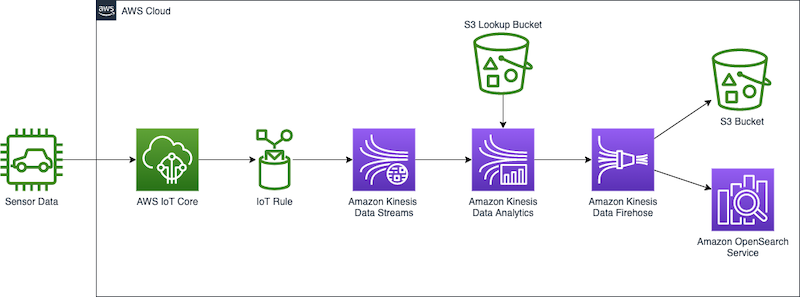
In our solution, we create a notebook to access automotive sensor data, enrich the data, and send the enriched output from the Kinesis Data Analytics Studio notebook to an Amazon Kinesis Data Firehose delivery stream for delivery to an Amazon Simple Storage Service (Amazon S3) data lake. This pipeline could further be used to send data to Amazon OpenSearch Service or other targets for additional processing and visualization.

Kinesis Data Analytics for SQL Applications vs. Kinesis Data Analytics for Apache Flink

In our example, we perform the following actions on the streaming data:

1. Connect to an Amazon Kinesis Data Streams data stream.
2. View the stream data.
3. Transform and enrich the data.
4. Manipulate the data with Python.
5. Restream the data to a Firehose delivery stream.

To compare Kinesis Data Analytics for SQL Applications with Kinesis Data Analytics for Apache Flink, let’s first discuss how Kinesis Data Analytics for SQL Applications works.

At the root of a Kinesis Data Analytics for SQL application is the concept of an in-application stream. You can think of the in-application stream as a table that holds the streaming data so you can perform actions on it. The in-application stream is mapped to a streaming source such as a Kinesis data stream. To get data into the in-application stream, first set up a source in the management console for your Kinesis Data Analytics for SQL application. Then, create a pump that reads data from the source stream and places it into the table. The pump query runs continuously and feeds the source data into the in-application stream. You can create multiple pumps from multiple sources to feed the in-application stream. Queries are then run on the in-application stream, and results can be interpreted or sent to other destinations for further processing or storage.

The following SQL demonstrates setting up an in-application stream and pump:

CREATE OR REPLACE STREAM "TEMPSTREAM" ( 
   "column1" BIGINT NOT NULL, 
   "column2" INTEGER, 
   "column3" VARCHAR(64));

CREATE OR REPLACE PUMP "SAMPLEPUMP" AS 
INSERT INTO "TEMPSTREAM" ("column1", 
                          "column2", 
                          "column3") 
SELECT STREAM inputcolumn1, 
      inputcolumn2, 
      inputcolumn3
FROM "INPUTSTREAM";

Data can be read from the in-application stream using a SQL SELECT query:

SELECT *
FROM "TEMPSTREAM"

When creating the same setup in Kinesis Data Analytics Studio, you use the underlying Apache Flink environment to connect to the streaming source, and create the data stream in one statement using a connector. The following example shows connecting to the same source we used before, but using Apache Flink:

CREATE TABLE `MY_TABLE` ( 
   "column1" BIGINT NOT NULL, 
   "column2" INTEGER, 
   "column3" VARCHAR(64)
) WITH (
   'connector' = 'kinesis',
   'stream' = sample-kinesis-stream',
   'aws.region' = 'aws-kinesis-region',
   'scan.stream.initpos' = 'LATEST',
   'format' = 'json'
 );

MY_TABLE is now a data stream that will continually receive the data from our sample Kinesis data stream. It can be queried using a SQL SELECT statement:

SELECT column1, 
       column2, 
       column3
FROM MY_TABLE;

Although Kinesis Data Analytics for SQL Applications use a subset of the SQL:2008 standard with extensions to enable operations on streaming data, Apache Flink’s SQL support is based on Apache Calcite, which implements the SQL standard.

It’s also important to mention that Kinesis Data Analytics Studio supports PyFlink and Scala alongside SQL within the same notebook. This allows you to perform complex, programmatic methods on your streaming data that aren’t possible with SQL.

Prerequisites

During this exercise, we set up various AWS resources and perform analytics queries. To follow along, you need an AWS account with administrator access. If you don’t already have an AWS account with administrator access, create one now. The services outlined in this post may incur charges to your AWS account. Make sure to follow the cleanup instructions at the end of this post.

Configure streaming data

In the streaming domain, we’re often tasked with exploring, transforming, and enriching data coming from Internet of Things (IoT) sensors. To generate the real-time sensor data, we employ the AWS IoT Device Simulator. This simulator runs within your AWS account and provides a web interface that lets users launch fleets of virtually connected devices from a user-defined template and then simulate them to publish data at regular intervals to AWS IoT Core. This means we can build a virtual fleet of devices to generate sample data for this exercise.

We deploy the IoT Device Simulator using the following Amazon CloudFront template. It handles creating all the necessary resources in your account.

1. On the Specify stack details page, assign a name to your solution stack.
2. Under Parameters, review the parameters for this solution template and modify them as necessary.
3. For User email, enter a valid email to receive a link and password to log in to the IoT Device Simulator UI.
4. Choose Next.
5. On the Configure stack options page, choose Next.
6. On the Review page, review and confirm the settings. Select the check boxes acknowledging that the template creates AWS Identity and Access Management (IAM) resources.
7. Choose Create stack.

The stack takes about 10 minutes to install.

8. When you receive your invitation email, choose the CloudFront link and log in to the IoT Device Simulator using the credentials provided in the email.

The solution contains a prebuilt automotive demo that we can use to begin delivering sensor data quickly to AWS.

9. On the Device Type page, choose Create Device Type.
10. Choose Automotive Demo.
11. The payload is auto populated. Enter a name for your device, and enter automotive-topic as the topic.
    
12. Choose Save.

Now we create a simulation.

13. On the Simulations page, choose Create Simulation.
14. For Simulation type, choose Automotive Demo.
15. For Select a device type, choose the demo device you created.
16. For Data transmission interval and Data transmission duration, enter your desired values.

You can enter any values you like, but use at least 10 devices transmitting every 10 seconds. You’ll want to set your data transmission duration to a few minutes, or you’ll need to restart your simulation several times during the lab.

17. Choose Save.
    

Now we can run the simulation.

18. On the Simulations page, select the desired simulation, and choose Start simulations.

Alternatively, choose View next to the simulation you want to run, then choose Start to run the simulation.

19. To view the simulation, choose View next to the simulation you want to view.

If the simulation is running, you can view a map with the locations of the devices, and up to 100 of the most recent messages sent to the IoT topic.

We can now check to ensure our simulator is sending the sensor data to AWS IoT Core.

20. Navigate to the AWS IoT Core console.

Make sure you’re in the same Region you deployed your IoT Device Simulator.

21. In the navigation pane, choose MQTT Test Client.
22. Enter the topic filter automotive-topic and choose Subscribe.

As long as you have your simulation running, the messages being sent to the IoT topic will be displayed.

Finally, we can set a rule to route the IoT messages to a Kinesis data stream. This stream will provide our source data for the Kinesis Data Analytics Studio notebook.

23. On the AWS IoT Core console, choose Message Routing and Rules.
24. Enter a name for the rule, such as automotive_route_kinesis, then choose Next.
    
25. Provide the following SQL statement. This SQL will select all message columns from the automotive-topic the IoT Device Simulator is publishing:

SELECT timestamp, trip_id, VIN, brake, steeringWheelAngle, torqueAtTransmission, engineSpeed, vehicleSpeed, acceleration, parkingBrakeStatus, brakePedalStatus, transmissionGearPosition, gearLeverPosition, odometer, ignitionStatus, fuelLevel, fuelConsumedSinceRestart, oilTemp, location 
FROM 'automotive-topic' WHERE 1=1

26. Choose Next.
27. Under Rule Actions, select Kinesis Stream as the source.
28. Choose Create New Kinesis Stream.

This opens a new window.

29. For Data stream name, enter automotive-data.

We use a provisioned stream for this exercise.

30. Choose Create Data Stream.

You may now close this window and return to the AWS IoT Core console.

31. Choose the refresh button next to Stream name, and choose the automotive-data stream.
    
32. Choose Create new role and name the role automotive-role.
33. Choose Next.
34. Review the rule properties, and choose Create.

The rule begins routing data immediately.

Set up Kinesis Data Analytics Studio

Now that we have our data streaming through AWS IoT Core and into a Kinesis data stream, we can create our Kinesis Data Analytics Studio notebook.

1. On the Amazon Kinesis console, choose Analytics applications in the navigation pane.
2. On the Studio tab, choose Create Studio notebook.
   
3. Leave Quick create with sample code selected.
4. Name the notebook automotive-data-notebook.
   
5. Choose Create to create a new AWS Glue database in a new window.
6. Choose Add database.
   
7. Name the database automotive-notebook-glue.
8. Choose Create.
   
9. Return to the Create Studio notebook section.
10. Choose refresh and choose your new AWS Glue database.
11. Choose Create Studio notebook.
    
12. To start the Studio notebook, choose Run and confirm.
    
13. Once the notebook is running, choose the notebook and choose Open in Apache Zeppelin.
14. Choose Import note.
15. Choose Add from URL.
    
16. Enter the following URL: https://aws-blogs-artifacts-public.s3.amazonaws.com/artifacts/BDB-2461/auto-notebook.ipynb.
17. Choose Import Note.
    
18. Open the new note.

Perform stream analysis

In a Kinesis Data Analytics for SQL application, we add our streaming course via the management console, and then define an in-application stream and pump to stream data from our Kinesis data stream. The in-application stream functions as a table to hold the data and make it available for us to query. The pump takes the data from our source and streams it to our in-application stream. Queries may then be run against the in-application stream using SQL, just as we’d query any SQL table. See the following code:

CREATE OR REPLACE STREAM "AUTOSTREAM" ( 
    `trip_id` CHAR(36),
    `VIN` CHAR(17),
    `brake` FLOAT,
    `steeringWheelAngle` FLOAT,
    `torqueAtTransmission` FLOAT,
    `engineSpeed` FLOAT,
    `vehicleSpeed` FLOAT,
    `acceleration` FLOAT,
    `parkingBrakeStatus` BOOLEAN,
    `brakePedalStatus` BOOLEAN,
    `transmissionGearPosition` VARCHAR(10),
    `gearLeverPosition` VARCHAR(10),
    `odometer` FLOAT,
    `ignitionStatus` VARCHAR(4),
    `fuelLevel` FLOAT,
    `fuelConsumedSinceRestart` FLOAT,
    `oilTemp` FLOAT,
    `location` VARCHAR(100),
    `timestamp` TIMESTAMP(3));

CREATE OR REPLACE PUMP "MYPUMP" AS 
INSERT INTO "AUTOSTREAM" ("trip_id",
    "VIN",
    "brake",
    "steeringWheelAngle",
    "torqueAtTransmission",
    "engineSpeed",
    "vehicleSpeed",
    "acceleration",
    "parkingBrakeStatus",
    "brakePedalStatus",
    "transmissionGearPosition",
    "gearLeverPosition",
    "odometer",
    "ignitionStatus",
    "fuelLevel",
    "fuelConsumedSinceRestart",
    "oilTemp",
    "location",
    "timestamp")
SELECT VIN,
    brake,
    steeringWheelAngle,
    torqueAtTransmission,
    engineSpeed,
    vehicleSpeed,
    acceleration,
    parkingBrakeStatus,
    brakePedalStatus,
    transmissionGearPosition,
    gearLeverPosition,
    odometer,
    ignitionStatus,
    fuelLevel,
    fuelConsumedSinceRestart,
    oilTemp,
    location,
    timestamp
FROM "INPUT_STREAM"

To migrate an in-application stream and pump from our Kinesis Data Analytics for SQL application to Kinesis Data Analytics Studio, we convert this into a single CREATE statement by removing the pump definition and defining a kinesis connector. The first paragraph in the Zeppelin notebook sets up a connector that is presented as a table. We can define columns for all items in the incoming message, or a subset.

Run the statement, and a success result is output in your notebook. We can now query this table using SQL, or we can perform programmatic operations with this data using PyFlink or Scala.

Before performing real-time analytics on the streaming data, let’s look at how the data is currently formatted. To do this, we run a simple Flink SQL query on the table we just created. The SQL used in our streaming application is identical to what is used in a SQL application.

Note that if you don’t see records after a few seconds, make sure that your IoT Device Simulator is still running.

If you’re also running the Kinesis Data Analytics for SQL code, you may see a slightly different result set. This is another key differentiator in Kinesis Data Analytics for Apache Flink, because the latter has the concept of exactly once delivery. If this application is deployed to production and is restarted or if scaling actions occur, Kinesis Data Analytics for Apache Flink ensures you only receive each message once, whereas in a Kinesis Data Analytics for SQL application, you need to further process the incoming stream to ensure you ignore repeat messages that could affect your results.

You can stop the current paragraph by choosing the pause icon. You may see an error displayed in your notebook when you stop the query, but it can be ignored. It’s just letting you know that the process was canceled.

Flink SQL implements the SQL standard, and provides an easy way to perform calculations on the stream data just like you would when querying a database table. A common task while enriching data is to create a new field to store a calculation or conversion (such as from Fahrenheit to Celsius), or create new data to provide simpler queries or improved visualizations downstream. Run the next paragraph to see how we can add a Boolean value named accelerating, which we can easily use in our sink to know if an automobile was currently accelerating at the time the sensor was read. The process here doesn’t differ between Kinesis Data Analytics for SQL and Kinesis Data Analytics for Apache Flink.

You can stop the paragraph from running when you have inspected the new column, comparing our new Boolean value to the FLOAT acceleration column.

Data being sent from a sensor is usually compact to improve latency and performance. Being able to enrich the data stream with external data and enrich the stream, such as additional vehicle information or current weather data, can be very useful. In this example, let’s assume we want to bring in data currently stored in a CSV in Amazon S3, and add a column named color that reflects the current engine speed band.

Apache Flink SQL provides several source connectors for AWS services and other sources. Creating a new table like we did in our first paragraph but instead using the filesystem connector permits Flink to directly connect to Amazon S3 and read our source data. Previously in Kinesis Data Analytics for SQL Applications, you couldn’t add new references inline. Instead, you defined S3 reference data and added it to your application configuration, which you could then use as a reference in a SQL JOIN.

NOTE: If you are not using the us-east-1 region, you can download the csv and place the object your own S3 bucket.  Reference the csv file as s3a://<bucket-name>/<key-name>

Building on the last query, the next paragraph performs a SQL JOIN on our current data and the new lookup source table we created.

Now that we have an enriched data stream, we restream this data. In a real-world scenario, we have many choices on what to do with our data, such as sending the data to an S3 data lake, another Kinesis data stream for further analysis, or storing the data in OpenSearch Service for visualization. For simplicity, we send the data to Kinesis Data Firehose, which streams the data into an S3 bucket acting as our data lake.

Kinesis Data Firehose can stream data to Amazon S3, OpenSearch Service, Amazon Redshift data warehouses, and Splunk in just a few clicks.

Create the Kinesis Data Firehose delivery stream

To create our delivery stream, complete the following steps:

1. On the Kinesis Data Firehose console, choose Create delivery stream.
2. Choose Direct PUT for the stream source and Amazon S3 as the target.
   
3. Name your delivery stream automotive-firehose.
   
4. Under Destination settings, create a new bucket or use an existing bucket.
5. Take note of the S3 bucket URL.
   
6. Choose Create delivery stream.

The stream takes a few seconds to create.

7. Return to the Kinesis Data Analytics console and choose Streaming applications.
8. On the Studio tab, and choose your Studio notebook.
   
9. Choose the link under IAM role.
   
10. In the IAM window, choose Add permissions and Attach policies.
    
11. Search for and select AmazonKinesisFullAccess and CloudWatchFullAccess, then choose Attach policy.
12. You may return to your Zeppelin notebook.

Stream data into Kinesis Data Firehose

As of Apache Flink v1.15, creating the connector to the Firehose delivery stream works similar to creating a connector to any Kinesis data stream. Note that there are two differences: the connector is firehose, and the stream attribute becomes delivery-stream.

After the connector is created, we can write to the connector like any SQL table.

To validate that we’re getting data through the delivery stream, open the Amazon S3 console and confirm you see files being created. Open the file to inspect the new data.

In Kinesis Data Analytics for SQL Applications, we would have created a new destination in the SQL application dashboard. To migrate an existing destination, you add a SQL statement to your notebook that defines the new destination right in the code. You can continue to write to the new destination as you would have with an INSERT while referencing the new table name.

Time data

Another common operation you can perform in Kinesis Data Analytics Studio notebooks is aggregation over a window of time. This sort of data can be used to send to another Kinesis data stream to identify anomalies, send alerts, or be stored for further processing. The next paragraph contains a SQL query that uses a tumbling window and aggregates total fuel consumed for the automotive fleet for 30-second periods. Like our last example, we could connect to another data stream and insert this data for further analysis.

Scala and PyFlink

There are times when a function you’d perform on your data stream is better written in a programming language instead of SQL, for both simplicity and maintenance. Some examples include complex calculations that SQL functions don’t support natively, certain string manipulations, the splitting of data into multiple streams, and interacting with other AWS services (such as text translation or sentiment analysis). Kinesis Data Analytics for Apache Flink has the ability to use multiple Flink interpreters within the Zeppelin notebook, which is not available in Kinesis Data Analytics for SQL Applications.

If you have been paying close attention to our data, you’ll see that the location field is a JSON string. In Kinesis Data Analytics for SQL, we could use string functions and define a SQL function and break apart the JSON string. This is a fragile approach depending on the stability of the message data, but this could be improved with several SQL functions. The syntax for creating a function in Kinesis Data Analytics for SQL follows this pattern:

CREATE FUNCTION ''<function_name>'' ( ''<parameter_list>'' )
    RETURNS ''<data type>''
    LANGUAGE SQL
    [ SPECIFIC ''<specific_function_name>''  | [NOT] DETERMINISTIC ]
    CONTAINS SQL
    [ READS SQL DATA ]
    [ MODIFIES SQL DATA ]
    [ RETURNS NULL ON NULL INPUT | CALLED ON NULL INPUT ]  
  RETURN ''<SQL-defined function body>''

In Kinesis Data Analytics for Apache Flink, AWS recently upgraded the Apache Flink environment to v1.15, which extends Apache Flink SQL’s table SQL to add JSON functions that are similar to JSON Path syntax. This allows us to query the JSON string directly in our SQL. See the following code:

%flink.ssql(type=update)
SELECT JSON_STRING(location, ‘$.latitude) AS latitude,
JSON_STRING(location, ‘$.longitude) AS longitude
FROM my_table

Alternatively, and required prior to Apache Flink v1.15, we can use Scala or PyFlink in our notebook to convert the field and restream the data. Both languages provide robust JSON string handling.

The following PyFlink code defines two user-defined functions, which extract the latitude and longitude from the location field of our message. These UDFs can then be invoked from using Flink SQL. We reference the environment variable st_env. PyFlink creates six variables for you in your Zeppelin notebook. Zeppelin also exposes a context for you as the variable z.

Errors can also happen when messages contain unexpected data. Kinesis Data Analytics for SQL Applications provides an in-application error stream. These errors can then be processed separately and restreamed or dropped. With PyFlink in Kinesis Data Analytics Streaming applications, you can write complex error-handling strategies and immediately recover and continue processing the data. When the JSON string is passed into the UDF, it may be malformed, incomplete, or empty. By catching the error in the UDF, Python will always return a value even if an error would have occurred.

The following sample code shows another PyFlink snippet that performs a division calculation on two fields. If a division-by-zero error is encountered, it provides a default value so the stream can continue processing the message.

%flink.pyflink
@udf(input_types=[DataTypes.BIGINT()], result_type=DataTypes.BIGINT())
def DivideByZero(price):    
	try:        
		price / 0        
	except:        
		return -1
st_env.register_function("DivideByZero", DivideByZero)

Next steps

Building a pipeline as we’ve done in this post gives us the base for testing additional services in AWS. I encourage you to continue your streaming analytics learning before tearing down the streams you created. Consider the following:

• Publish your Kinesis Data Analytics Studio notebook as an application with durable state.
• Use your Kinesis Data Firehose delivery stream to write directly to OpenSearch Service.
• Use OpenSearch Dashboards to visualize your streaming data.
• Review the Migrating to Kinesis Data Analytics for Apache Flink: Examples docs for side-by-side translations of common SQL-based Kinesis Data Analytics application queries to Kinesis Data Analytics Studio.

Clean up

To clean up the services created in this exercise, complete the following steps:

1. Navigate to the CloudFormation Console and delete the IoT Device Simulator stack.
2. On the AWS IoT Core console, choose Message Routing and Rules, and delete the rule automotive_route_kinesis.
3. Delete the Kinesis data stream automotive-data in the Kinesis Data Stream console.
4. Remove the IAM role automotive-role in the IAM Console.
5. In the AWS Glue console, delete the automotive-notebook-glue database.
6. Delete the Kinesis Data Analytics Studio notebook automotive-data-notebook.
7. Delete the Firehose delivery stream automotive-firehose.

Conclusion

Thanks for following along with this tutorial on Kinesis Data Analytics Studio. If you’re currently using a legacy Kinesis Data Analytics Studio SQL application, I recommend you reach out to your AWS technical account manager or Solutions Architect and discuss migrating to Kinesis Data Analytics Studio. You can continue your learning path in our Amazon Kinesis Data Streams Developer Guide, and access our code samples on GitHub.

About the Author

Nicholas Tunney is a Partner Solutions Architect for Worldwide Public Sector at AWS. He works with global SI partners to develop architectures on AWS for clients in the government, nonprofit healthcare, utility, and education sectors.