Post Syndicated from BeardedTinker original https://www.youtube.com/watch?v=C_xttj4wncQ
Center for Information Security (CIS) unveils Azure Foundations Benchmark v2.0.0
Post Syndicated from Marla Rosner original https://blog.rapid7.com/2023/03/23/center-for-information-security-cis-unveils-azure-foundations-benchmark-v2-0-0/

The Center for Information Security (CIS) recently unveiled the latest version of their Azure Foundations Benchmark—Version 2.0.0. This is the first major release since the benchmark was originally released more than 4 years ago, which could lead you to believe that this update would come with a bunch of significant changes. However, this release actually brings fewer impactful changes than the minor releases that preceded it.
Instead of sweeping changes, the update includes a number of reconciled and renumbered sections along with some refreshed language and branding.
Rapid7 is actively reviewing the new recommendations and evaluating the need and potential of them being made into insights within InsightCloudSec.
So the changes were minor, but what were they?
Of the 10 sections that make up the benchmark, four sections were expanded with new recommendations:
- Section 1 (Identity and Access Management)
- This was also the only section that had a recommendation removed.
- Section 4 (Database Services)
- Section 5 (Logging and Monitoring)
- Section 7 (Virtual Machines)
Five sections had no changes:
- Section 3 (Storage Accounts)
- Section 6 (Networking)
- Section 8 (Key Vault)
- Section 9 (AppService)
- Section 10 (Miscellaneous)
Section 2 (Microsoft Defender) did not have any additions or subtractions, but did have some alterations related to numbering and categorization.
Section 1 (Identity and Access Management)
This section covers a wide range of recommendations centered around identity and access policies. For 2.0.0, there was one addition:
Recommendation: 1.3 – Ensure that ‘Users can create Azure AD Tenants’ is set to ‘No’
Why it Matters: It is best practice to only allow an administrator to create new tenants. This prevents users from creating new Azure AD or Azure AD B2C tenants and ensures that only authorized users are able to do so.
As noted above, this was also the only section from which a recommendation was removed entirely:
Removed Recommendation: 1.5 – Ensure that ‘Restore multi-factor authentication on all remembered devices’ is enabled (this recommendation has been replaced in v2.0.0)
Why it Was Removed: This recommendation was likely removed, as it is somewhat redundant to what is now recommendation 1.1.4 (Ensure that ‘Allow users to remember multi-factor authentication on devices they trust’ is enabled). Essentially, the updated recommendation asserts you should not allow users to bypass MFA for any device.
Section 4 (Database Services)
This section focuses on securing database services within Azure environments—such as Azure SQL or Cosmos DB. CIS added a recommendation to this section, specifically for Cosmos DB, that guides users to leverage Active Directory and Azure RBAC whenever possible.
Recommendation: 4.5.3 – Use Azure Active Directory (AAD) Client Authentication and Azure RBAC where possible.
Why it Matters: Cosmos DB, Azure’s native NoSQL database service, can use tokens or AAD for client authentication which in turn will use Azure RBAC for authorization. Using AAD is significantly more secure because AAD handles the credentials and allows for MFA and centralized management, and Azure RBAC is better integrated with the rest of Azure.
Section 5 (Logging and Monitoring)
The two new recommendations within this section are targeted toward ensuring you’ve properly configured your environment for log management, including collecting the necessary logs (flow logs, audit logs, activity logs, etc.) and also ensuring that the storage location for those logs is secure.
Recommendation: 5.3.1 – Ensure Application Insights are Configured
Why it Matters: Application Insights within Azure act as an application performance monitoring solution providing valuable data into how well an application performs and additional information when performing incident response. The types of log data collected include application metrics, telemetry data, and application trace logging data, which provide organizations with detailed information about application activity and application transactions. Both data sets help organizations adopt a proactive and retroactive means to handle security and performance related metrics within their modern applications.
Recommendation: 5.5 – Ensure that SKU Basic/Consumption is not used on artifacts that need to be monitored
Why it Matters: Basic or Free SKUs in Azure, while cost effective, have significant limitations in terms of what can be monitored and what support can be realized from the team at Microsoft. Typically, these SKU’s do not have service SLAs, and Microsoft generally refuses to provide support for them. Because of this, Basic/Free SKUs are not recommended for production workloads. While upgrading to the Standard tier may be a bit more expensive, you’ll receive more support from Microsoft, as well as the ability to generate and consume more detailed information via native monitoring services such as Azure Monitor.
Section 7 (Virtual Machines)
Section 7 is focused on securing virtual machines within your Azure environment. Recommendations in this section include ensuring that your VMs are utilizing managed disks and that OS and Data disks are encrypted with Customer Managed Keys (CMK), just to name a few. There was one new recommendation in this section.
Recommendation: 7.1 – Ensure an Azure Bastion Host Exists
Why it Matters: The Azure Bastion service allows organizations a more secure means of accessing Azure Virtual Machines over the Internet without assigning public IP addresses to them. The Azure Bastion service provides Remote Desktop Protocol (RDP) and Secure Shell (SSH) access to Virtual Machines using TLS within a web browser. This is aimed at preventing organizations from opening up 3389/TCP and 22/TCP to the Internet on Azure Virtual Machines.
Using InsightCloudSec to Implement and Enforce CIS Azure Foundations Benchmark 2.0.0
InsightCloudSec continuously assesses your entire cloud environment—whether single cloud or hosted across multiple platforms—for compliance with organizational standards. It detects noncompliant resources and unapproved changes within minutes. The platform continuously monitors your environment to ensure you’ve properly implemented the necessary controls as recommended by CIS for securing your cloud workloads running in Azure environments.
InsightCloudSec can instantly detect whenever an account or resource drifts from compliance. The platform comes out of the box with 30+ compliance packs, including a dedicated pack for the CIS Azure Foundations Benchmark 2.0.0. A compliance pack within InsightCloudSec is a set of checks that can be used to continuously assess your cloud environments for compliance with a given regulatory framework, or industry or provider best practices.
As you can see in the screenshot below, InsightCloudSec has a host of checks and insights that directly align to recommendations within the CIS Azure Foundations Benchmark 2.0.0.

When you dive deeper into a given insight, you’re provided with detail into how many resources are in violation with a given check and a relative risk score to outline just how risky a given violation is.
Below is an example from CIS Azure Foundations Benchmark 2.0.0, specifically a set of resources that are in violation of the check ‘Storage Account Older than 90 Days Without Access Keys Rotated’. You’re provided with an overview of the insight, including why it’s important to implement and the risks associated with not doing so.

That platform doesn’t just stop there, however. You’re also provided with the necessary remediation steps as advised by CIS themselves, and if you so choose, the recommended automations that can be created using native bots within InsightCloudSec for folks that would prefer to completely remove the human effort involved in enforcing compliance with this policy.

If you’re interested in learning more about how InsightCloudSec helps continuously and automatically enforce cloud security standards, be sure to check out the demo!
Proxmox VE 7.4 Released with Dark Mode Support
Post Syndicated from Cliff Robinson original https://www.servethehome.com/proxmox-ve-7-4-released-with-dark-mode-support/
Proxmox VE 7.4 is out, now with Dark Mode support (FINALLY) and several other updates and features to the popular virtualization platform
The post Proxmox VE 7.4 Released with Dark Mode Support appeared first on ServeTheHome.
Object Storage for Film, Video, and Content Creation
Post Syndicated from James Flores original https://www.backblaze.com/blog/object-storage-for-film-video-and-content-creation/
Twenty years ago, who would have thought going to work would mean spending most of your time on a computer and running most of your applications through a web browser or a mobile app? Today, we can do everything remotely via the power of the internet—from email to gaming, from viewing our home security cameras to watching the latest and greatest movie trailers—and we all have opinions about the best browsers, too…
Along with that easy, remote access, a slew of new cloud technologies are fueling the tech we use day in and day out. To get to where we are today, the tech industry had to rethink some common understandings, especially around data storage and delivery. Gone are the days that you save a file on your laptop, then transport a copy of that file via USB drive or CD-ROM (or, dare we say, a floppy disk) so that you can keep working on it at the library or your office. And, those same common understandings are now being reckoned with in the world of film, video, and content creation.
In this post, I’ll dive into storage, specifically cloud object storage, and what it means for the future of content creation, not only for independent filmmakers and content creators, but also in post-production workflows.
The Evolution of File Management
If you are reading this blog you are probably familiar with a storage file system—think Windows Explorer, the Finder on Mac, or directory structures in Linux. You know how to create a folder, create files, move files, and delete folders. This same file structure has made its way into cloud services such as Google Drive, Box, and Dropbox. And many of these technologies have been adopted to store some of the largest content, namely media files like .mp4, .wav, or .r3d files.
But, as camera file outputs grow larger and larger and the amount of content generated by creative teams soars, folders structures get more and more complex. Why is this important?
Well, ask yourself: How much time have you spent searching for clips you know exist, but just can’t seem to find? Sure, you can use search tools to search your folder structure but as you have more and more content, that means searching for the proverbial needle in a haystack—naming conventions can only do so much, especially when you have dozens or hundreds of people adding raw footage, creating new versions, and so on.
Finding files in a complex file structure can take so much time that many of the aforementioned companies create system limits preventing long searches. In addition, they may limit uploads and downloads making it difficult to manage the terabytes of data a modern production creates. So, this all begs the question: Is a traditional file system really the best for scaling up, especially in data-heavy industries like filmmaking and video content creation? Enter: Cloud object storage.
Refresher: What is Object Storage?
You can think of object storage as simply a big pool of storage space filled with object data. In the past we’ve defined object data as “some assemblage of data with one unique identifier and an infinite amount of metadata.” The three components that comprise objects in object storage are key here. They include:
- Unique Identifier: Referred to as a universally unique identifier (UUID) or global unique identifier (GUID), this is simply a complex number identifier.
- Infinite Metadata: Data about the data with endless possibilities.
- Data: The actual data we are storing.
So what does that actually mean?
It means each object (this can be any type of file—a .jpg, .mp4, .wav, .r3d, etc.) has an automatically generated unique identifier which is just a number (e.g. 4_z6b84cf3535395) versus a folder structure path you must manually create and maintain (e.g. D:\Projects\JOB4548\Assets\RAW\A001\A001_3424OP.RDM\A001_34240KU.RDC\
A001_A001_1005ku_001.R3D).

It also means each object can have an infinite amount of metadata attached to it. Metadata, put simply, is a “tag” that identifies how the file is used or stored. There are several examples of metadata, but here are just a few:
- Descriptive metadata, like the title or author.
- Structural metadata, like how to order pages in a chapter.
- Administrative metadata, like when the file was created, who has permissions to it, and so on.
- Legal metadata, like who holds the copyright or if the file is in the public domain.
So, when you’re saying an image file is 400×400 pixels and in .jpg format, you’ve just identified two pieces of metadata about the file. In filmmaking, metadata can include things like reel numbers or descriptions. And, as artificial intelligence (AI) and machine learning tools continue to evolve, the amount of metadata about a given piece of footage or image only continues to grow. AI tools can add data around scene details, facial recognition, and other identifiers, and since those are coded as metadata, you will be able to store and search files using terms like “scenes with Bugs Bunny” or “scenes that are in a field of wildflowers”—and that means that you’ll spend less time trying to find the footage you need when you’re editing.
When you put it all together, you have one gigantic content pool that can grow infinitely. It uses no manually created complex folder structure and naming conventions. And it can hold an infinite amount of data about your data (metadata), making your files more discoverable.
Let’s Talk About Object Storage for Content Creation
You might be wondering: What does this have to do with the content I’m creating?
Consider this: When you’re editing a project, how much of your time is spent searching for files? A recent study by GISTICS found that the average creative person searches for media 83 times a week. Maybe you’re searching your local hard drive first, then your NAS, then those USB drives in your closet. Or, maybe you are restoring content off an LTO tape to search for that one clip you need. Or, maybe you moved some of your content to the cloud—is it in your Google Drive or in your Dropbox account? If so, which folder is it in? Or was it the corporate Box account? Do you have permissions to that folder? All of that complexity means that the average creative person fails to find the media they are looking for 35% of the time. But you probably don’t need a study to tell you we all spent huge amounts of time searching for content.

Here is where object storage can help. With object storage, you simply have buckets (object storage containers) where all your data can live, and you can access it from wherever you’re working. That means all of the data stored on those shuttle drives sitting around your office, your closet of LTO tapes, and even a replica of your online NAS are in a central, easily accessible location. You’re also working from the most recent file.
Once it’s in the cloud, it’s safe from the types of disasters that affect on-premises storage systems, and it’s easy to secure your files, create backups, and so on. It’s also readily available when you need it, and much easier to share with other team members. It’s no wonder many of the apps you use today take advantage of object storage as their primary storage mechanism.
The Benefits of Object Storage for Media Workflows
Object storage offers a number of benefits for creative teams when it comes to streamlining workflows, including:
- Instant access
- Integrations
- Workflow interoperability
- Easy distribution
- Off-site back up and archive
Instant Access
With cloud object storage, content is ready when you need it. You know inspiration can strike at any time. You could be knee deep in editing a project, in the middle of binge watching the latest limited series, or out for a walk. Whenever the inspiration decides to strike, having instant access to your library of content is a game changer. And that’s the great thing about object storage in the cloud: you gain access to massive amounts of data with a few clicks.
Integrations
Object storage is a key component of many of the content production tools in use today. For example, iconik is a cloud-native media asset management (MAM) tool that can gather and organize media from any storage location. You can point iconik to your Backblaze B2 Bucket and use its advanced search functions as well as its metadata tagging.
Workflow Interoperability
What if you don’t want to use iconik, specifically? What’s great about using cloud storage as a centralized repository is that no matter what application you use, your data is in a single place. Think of it like your external hard drive or NAS—you just connect that drive with a new tool, and you don’t have to worry about downloading everything to move to the latest and greatest. In essence, you are bringing your own storage (BYOS!).
Here’s an example: CuttingRoom is a cloud native video editing and collaboration tool. It runs entirely in your web browser and lets you create unique stories that can instantly be published to your destination of choice. What’s great about CuttingRoom is its ability to read an object storage bucket as a source. By simply pointing CuttingRoom to a Backblaze B2 Bucket, it has immediate access to the media source files and you can get to editing. On the other hand, if you prefer using a MAM, that same bucket can be indexed by a tool like iconik.
Easy Distribution
Now that your edit is done, it’s time to distribute your content to the world. Or, perhaps you are working with other teams to perfect your color and sound, and it’s time to share your picture lock version. Cloud storage is ready for you to distribute your files to the next team or an end user.
Here’s a recent, real-world example: If you have been following the behind-the-scenes articles about creating Avatar: The Way of Water, you know that not only was its creation the spark of new technology like the Sony Venice camera with removable sensors, but the distribution featured a cloud centric flow. Footage (the film) was placed in an object store (read: a cloud storage database), processed into different formats, languages were added with 3D captions, and then footage was distributed directly from a central location.
And, while not all of us have Jon Landau as our producer, a huge budget, and a decade to create our product, this same flexibility exists today with object storage—with the added bonus that it’s usually budget-friendly as well.
Off-Site Back Up and Archive
And last but certainly not least, let’s talk back up and archive. Once a project is done, you need space for the next project, but no one wants to risk losing the old project. Who out there is completely comfortable hitting the delete key as well as saying yes to the scary prompt, “Are you sure you want to delete?”
Well, that’s what you would have to do in the past. These days, object storage is a great place to store your terabytes and terabytes of archived footage without cluttering your home, office, or set with additional hardware. Compared with on-premises storage, cloud storage lets you add more capacity as you need it—just make sure you understand cloud storage pricing models so that you’re getting the best bang for your buck.
If you’re using a NAS device in your media workflow, you’ll find you need to free up your on-prem storage. Many NAS devices, like Synology and QNAP, have cloud storage integrations that allow you to automatically sync and archive data from your device to the cloud. In fact, you could start taking advantage of this today.
No delete key here—just a friendly archive button.
Getting Started With Object Storage for Media Workflows
Migrating to the cloud may seem daunting, but it doesn’t have to be. Especially with the acceleration of hybrid workflows in the film industry recently, cloud-based workflows are becoming more common and better integrated with the tools we use every day. You can test this out with Backblaze using your free 10GB that you get just for signing up for Backblaze B2. Sure, that may not seem like much when a single .r3d file is 4GB. But with that 10GB, you can test upload speeds and download speeds, try out integrations with your preferred workflow tools, and experiment with AI metadata. If your team is remote, you could try an integration with LucidLink. Or if you’re looking to power a video on-demand site, you could integrate with one of our content delivery network (CDN) partners to test out content distribution, like Backblaze customer Kanopy, a streaming service that delivers 25,000 videos to libraries worldwide.
Change is hard, but cloud storage can be easy. Check out all of our media workflow solutions and get started with your 10GB free today.
The post Object Storage for Film, Video, and Content Creation appeared first on Backblaze Blog | Cloud Storage & Cloud Backup.
Reduce Risk and Regain Control with Cloud Risk Complete
Post Syndicated from Marla Rosner original https://blog.rapid7.com/2023/03/23/reduce-risk-and-regain-control-with-cloud-risk-complete/

Over the last 10 to 15 years, organizations have been migrating to the cloud to take advantage of the speed and scale it enables. During that time, we’ve all had to learn that new cloud infrastructure means new security challenges, and that many legacy tools and processes are unable to keep up with the new pace of innovation.
The greater scale, complexity, and rate of change associated with modern cloud environments means security teams need more control to effectively manage organizational risk. Traditional vulnerability management (VM) tools are not designed to keep pace with highly dynamic cloud environments, creating coverage gaps that increase risk and erode confidence.
In the report “Forecast Analysis: Cloud Infrastructure and Platform Services, Worldwide” Gartner® estimates that “By 2025, more than 90% of enterprise cloud infrastructure and platform environments will be based on a CIPS [cloud infrastructure and platform services] offering from one of the top four public cloud hyperscale providers, up from 75% to 80% in 2021.”
In the face of all this rapid change, how do you keep up?
Rapid7’s Cloud Risk Complete Is Here
The future of risk management is seamless coverage across your entire environment. That’s why our new offer, Cloud Risk Complete, is the most comprehensive solution to detect and manage risk across cloud environments, endpoints, on-premises infrastructure, and web applications.
With Cloud Risk Complete, you can:
- Gain unlimited risk coverage with a unified solution purpose-built for hybrid environments, providing continuous visibility into your on-prem infrastructure, cloud, and apps, all in a single subscription.
- Make context-driven decisions by intelligently prioritizing risk based on context from every layer of your attack surface, driven by a real risk score that ties risk to business impact.
- Enable practitioner-first collaboration with native, no-code automation to help teams work more efficiently and executive-level dashboards that provide visibility into your risk posture.
Cloud Risk Complete
Analyze, respond to, and remediate risks without a patchwork of solutions or additional costs.
What makes this solution different is that we started with the outcome and worked backwards to bring to life a solution that meets the needs of your security program.
- While most solutions offer daily scans of your cloud environment, we deliver real-time visibility into everything running across your environment. So, you’re never working with stale data or running blind.
- While most solutions only provide insight into a small portion of your environment, we provide a unified view of risk across your entire estate, including your apps, both in the cloud and on-prem.
- While most solutions show you a risk signal and leave the analysis and remediation process up to you, we provide step-by-step guidance on how to remediate the issue, and can even take immediate action with automated workflows that remove manual effort and accelerate response times.
Risk Is Pervasive. Your Cloud Security Should Be Too
Cloud Risk Complete stands apart from the pack with best-in-class cloud vulnerability assessment and management, cloud security posture management, cloud detection and response, and automation—in a single subscription.
Unlimited ecosystem automation enables your team to collaborate more effectively, improve the efficiency of your risk management program, and save time. With all of this, you can eliminate multiple contracts and vendors that are stretching budgets and enjoy a higher return on investment.
Get comprehensive cloud risk coverage across your business—without compromise. Discover Cloud Risk Complete today.
[$] Free software during wartime
Post Syndicated from original https://lwn.net/Articles/926798/
Just over 27 years ago, John Perry Barlow’s declaration of the
independence of Cyberspace claimed that governments “have no
” over the networked world. In 2023, we have ample reason
sovereignty
to know better than that, but we still expect the free-software community
to be left alone by the affairs of governments much of the time. A couple
of recent episodes related to the war in Ukraine are making it clear that
there are limits to our independence.
Kubernetes monitoring with Zabbix – Part 3: Extracting Prometheus metrics with Zabbix preprocessing
Post Syndicated from Michaela DeForest original https://blog.zabbix.com/kubernetes-monitoring-with-zabbix-part-3-extracting-prometheus-metrics-with-zabbix-preprocessing/25639/
In the previous Kubernetes monitoring blog post, we explored the functionality provided by the Kubernetes integration in Zabbix and discussed use cases for monitoring and alerting to events in a cluster, such as changes in replicas or CPU pressure.
In the final part of this series on monitoring Kubernetes with Zabbix, we will show how the Kubernetes integration uses Prometheus to parse data from kube-state-metrics and how users can leverage this functionality to monitor the many cloud-native applications that expose Prometheus metrics by default.
Want to see Kubernetes monitoring in action? Watch Part 3 of our Kubernetes monitoring video guide.
Prometheus Data Model
Prometheus is an open-source toolkit for monitoring and alerting created by SoundCloud. Prometheus was the second hosted project to join the Cloud-native Computing Foundation in 2016, after Kubernetes. As such, users of Kubernetes have adopted Prometheus extensively.
Lines in the model begin with or without a pound sign. Lines beginning with a pound sign specify metadata that includes help text and type information. Additional lines follow where the first key is the metric name with optional labels specified, followed by the value, and optionally concluding with a timestamp. If a timestamp is absent, the assumption is that the timestamp is equal to the time of collection.
http_requests_total{job=”nginx”,instance=”10.0.0.1:443”} 15 1677507349983
Using Prometheus with Kubernetes Monitoring
Let’s start with an example from the kube-state-metrics endpoint, installed in the first part of this series. Below is the output for the /metrics endpoint used by the Kubernetes integration, showing the metric kube_job_created. Each metric has help text followed by a line starting with that metric name, labels describing each job, and creation time as the sample value.
# HELP kube_job_created Unix creation timestamp
# TYPE kube_job_created gauge
kube_job_created{namespace="jdoe",job_name="supportreport-supportreport-27956880"} 1.6774128e+09
kube_job_created{namespace="default",job_name="core-backup-data-default-0-27957840"} 1.6774704e+09
kube_job_created{namespace="default",job_name="core-backup-data-default-1-27956280"} 1.6773768e+09
kube_job_created{namespace="jdoe",job_name="activetrials-activetrials-27958380"} 1.6775028e+09
kube_job_created{namespace="default",job_name="core-cache-tags-27900015"} 1.6740009e+09
kube_job_created{namespace="default",job_name="core-cleanup-pipes-27954860"} 1.6772916e+09
kube_job_created{namespace="jdoe",job_name="salesreport-salesreport-27954060"} 1.6772436e+09
kube_job_created{namespace="default",job_name="core-correlation-cron-1671562914"} 1.671562914e+09
kube_job_created{namespace="jtroy",job_name="jtroy-clickhouse-default-0-maintenance-27613440"} 1.6568064e+09
kube_job_created{namespace="default",job_name="core-backup-data-default-0-27956880"} 1.6774128e+09
kube_job_created{namespace="default",job_name="core-cleanup-sessions-27896445"} 1.6737867e+09
kube_job_created{namespace="default",job_name="report-image-findings-report-27937095"} 1.6762257e+09
kube_job_created{namespace="jdoe",job_name="salesreport-salesreport-27933900"} 1.676034e+09
kube_job_created{namespace="default",job_name="core-cache-tags-27899775"} 1.6739865e+09
kube_job_created{namespace="ssmith",job_name="test-auto-merger"} 1.653574763e+09
kube_job_created{namespace="default",job_name="report-image-findings-report-1650569984"} 1.650569984e+09
kube_job_created{namespace="ssmith",job_name="auto-merger-and-mailer-auto-merger-and-mailer-27952200"} 1.677132e+09
kube_job_created{namespace="default",job_name="core-create-pipes-pxc-user"} 1.673279381e+09
kube_job_created{namespace="jdoe",job_name="activetrials-activetrials-1640610000"} 1.640610005e+09
kube_job_created{namespace="jdoe",job_name="salesreport-salesreport-27943980"} 1.6766388e+09
kube_job_created{namespace="default",job_name="core-cache-accounting-map-27958085"} 1.6774851e+09
Zabbix collects data from this endpoint in the “Get state metrics.” The item uses a script item type to get data from the /metrics endpoint. Dependent items that use a Prometheus pattern as a preprocessing step to obtain data relevant to the dependent item are created.
Prometheus and Out-Of-The-Box Templates
Zabbix also offers many templates for applications that expose Prometheus metrics, including etcd. Etcd is a distributed key-value store that uses a simple HTTP interface. Many cloud applications use etcd, including Kubernetes. Following is a description of how to set up an etcd “host” using the built-in etcd template.
A new host is created called “Etcd Application” with an agent interface specified that provides the location of the application API. The interface port does not matter because a macro sets the port. The “Etcd by HTTP” template is attached to the host.

The “Get node metrics” item is the master item that collects Prometheus metrics. Testing this item shows that it returns Prometheus formatted metrics. The master item creates many dependent items that parse the Prometheus metrics. In the dependent item, “Maximum open file descriptors,” the maximum number of open file descriptors is obtained by adding the “Prometheus pattern” preprocessing step. This metric is available with the metric name process_max_fds.

Custom Prometheus Templates
While it is convenient when Zabbix has a template for the application you want to monitor, creating a new template for an application that exposes a /metrics endpoint but does not have an associated template is easy.
One such application is Argo CD. Argo CD is a GitOps continuous delivery tool for Kubernetes. An “application” represents each deployment in Kubernetes. Argo CD uses Git to keep applications in sync.
Argo CD exposes a Prometheus metrics endpoint that we can be used to monitor the application. The Argo CD documentation site includes information about available metrics.
In Argo CD, the metrics service is available at the argocd-metrics service. Following is a demonstration of creating an Argo CD template that collects Prometheus metrics. Install Argo CD in a cluster with a Zabbix proxy installed before starting. To do this, follow the Argo CD “Getting Started” guide.
Create a new template called, “Argo CD by HTTP” in the “Templates/Applications” group. Add three macros to the template. Set {$ARGO.METRICS.SERVICE.PORT} to the default of 8082. Set {$ARGO.METRICS.API.PATH} to “/metrics.” Set the last macro, {$ARGO.METRICS.SCHEME} to the default of “http.”
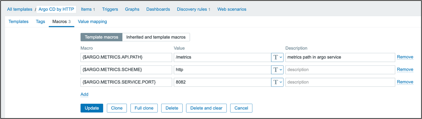
Open the template and click “Items -> Create item.” Name this item “Get Application Metrics” and give it the “HTTP agent” type. Set the key to argocd.get_metrics with a “Text” information type. Set the URL to {$ARGO.METRICS.SCHEME}://{HOST.CONN}:{$ARGO.METRICS.SERVICE.PORT}/metrics. Set the History storage period to “Do not keep history.”

Create a new host to represent Argo. Go to “Hosts -> Create host”. Name the host “Argo CD Application” and assign the newly created template. Define an interface and set the DNS name to the name of the metrics service, including the namespace, if the Argo CD deployment is not in the same namespace as the Zabbix proxy deployment. Connect to DNS and leave the port as the default because the template does not use this value. Like in the etcd template, a macro sets the port. Set the proxy to the proxy located in the cluster. In most cases, the macros do not need to be updated.
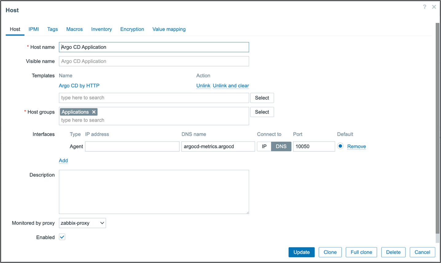
Click “Test -> Get value and test” to test the item. Prometheus metrics are returned, including a metric called argocd_app_info. This metric collects the status of the applications in Argo. We can collect all deployed applications with a discovery rule.

Navigate to the Argo CD template and click “Discovery rules -> Create discovery rule.” Call the rule “Discover Applications.” The type should be “Dependent item” because it depends on the metrics collection item. Set the master item to the “Get Application Metrics” item. The key will be argocd.applications.discovery. Go to the preprocessing tab and add a new step called, “Prometheus to JSON.” The preprocessing step will convert the application data to JSON, which will look like the one below.
[{"name":"argocd_app_info","value":"1","line_raw":"argocd_app_info{dest_namespace=\"monitoring\",dest_server=\"https://kubernetes.default.svc\",health_status=\"Healthy\",name=\"guestbook\",namespace=\"argocd\",operation=\"\",project=\"default\",repo=\"https://github.com/argoproj/argocd-example-apps\",sync_status=\"Synced\"} 1","labels":{"dest_namespace":"monitoring","dest_server":"https://kubernetes.default.svc","health_status":"Healthy","name":"guestbook","namespace":"argocd","operation":"","project":"default","repo":"https://github.com/argoproj/argocd-example-apps","sync_status":"Synced"},"type":"gauge","help":"Information about application."}]
Set the parameters to “argocd_app_info” to gather all metrics with that name. Under “LLD Macros”, set three macros. {#NAME} is set to the .labels.name key, {#NAMESPACE} is set to the .labels.dest_namespace key, and {#SERVER} is set to .labels.dest_server.

Let us create some item prototypes. Click “Create item prototype” and name it “{#NAME}: Health Status.” Set it as a dependent item with a key of argocd.applications[{#NAME}].health. The type of information will be “Character.” Set the master item to “Get Application Metrics.”
In preprocessing, add a Prometheus pattern step with parameters argocd_app_info{name=”{#NAME}”}. Use “label” and set the label to health_status. Add a second step to “Discard unchanged with heartbeat” with the heartbeat set to 2h.

Clone the prototype to create another item called “{#NAME}: Sync status.” Change the key to argocd.applications.sync[{#NAME}]. Under “Preprocessing” change the label to sync_status.
Now, when viewing “Latest Data” the sync and health status are available for each discovered application.

Conclusion
We have shown how Zabbix templates, such as the Kubernetes template, and the etcd template utilize Prometheus patterns to extract metric data. We have also created templates for new applications that expose Prometheus data. Because of the adoption of Prometheus in Kubernetes and cloud-native applications, Zabbix benefits by parsing this data so that Zabbix can monitor Kubernetes and cloud-native applications.
I hope you enjoyed this series on monitoring Kubernetes and cloud-native applications with Zabbix. Good luck on your monitoring journey as you learn to monitor with Zabbix in a containerized world.
About the Author
Michaela DeForest is a Platform Engineer for The ATS Group. She is a Zabbix Certified Specialist on Zabbix 6.0 with additional areas of expertise, including Terraform, Amazon Web Services (AWS), Ansible, and Kubernetes, to name a few. As ATS’s resident authority in DevOps, Michaela is critical in delivering cutting-edge solutions that help businesses improve efficiency, reduce errors, and achieve a faster ROI.
About ATS Group:
The ATS Group provides a fully inclusive set of technology services and tools designed to innovate and transform IT. Their systems integration, business resiliency, cloud enablement, infrastructure intelligence, and managed services help businesses of all sizes “get IT done.” With over 20 years in business, ATS has become the trusted advisor to nearly 500 customers across multiple industries. They have built their reputation around honesty, integrity, and technical expertise unrivaled by the competition.
The Ultimate Cheap Fanless 2.5GbE Switch Mega Round-Up
Post Syndicated from Patrick Kennedy original https://www.servethehome.com/the-ultimate-cheap-2-5gbe-switch-mega-round-up-qnap-netgear-hasivo-mokerlink-trendnet-zyxel-tp-link/
We test 15+ fanless 2.5GbE switches to see which are the top picks, which have cool features, and which ones are simply overpriced
The post The Ultimate Cheap Fanless 2.5GbE Switch Mega Round-Up appeared first on ServeTheHome.
Nikkor 85mm f1.2Z – Worth the price, size & weight??
Post Syndicated from Matt Granger original https://www.youtube.com/watch?v=9n9SIF74hks
Security updates for Thursday
Post Syndicated from original https://lwn.net/Articles/926972/
Security updates have been issued by CentOS (firefox, nss, and openssl), Fedora (firefox, liferea, python-cairosvg, and tar), Oracle (openssl and thunderbird), Scientific Linux (firefox, nss, and openssl), SUSE (container-suseconnect, grub2, libplist, and qemu), and Ubuntu (amanda, apache2, node-object-path, and python-git).
Out now! Auto-renew TLS certifications with DCV Delegation
Post Syndicated from Dina Kozlov original https://blog.cloudflare.com/introducing-dcv-delegation/


To get a TLS certificate issued, the requesting party must prove that they own the domain through a process called Domain Control Validation (DCV). As industry wide standards have evolved to enhance security measures, this process has become manual for Cloudflare customers that manage their DNS externally. Today, we’re excited to announce DCV Delegation — a feature that gives all customers the ability offload the DCV process to Cloudflare, so that all certificates can be auto-renewed without the management overhead.
Security is of utmost importance when it comes to managing web traffic, and one of the most critical aspects of security is ensuring that your application always has a TLS certificate that’s valid and up-to-date. Renewing TLS certificates can be an arduous and time-consuming task, especially as the recommended certificate lifecycle continues to gradually decrease, causing certificates to be renewed more frequently. Failure to get a certificate renewed can result in downtime or insecure connection which can lead to revenue decrease, mis-trust with your customers, and a management nightmare for your Ops team.
Every time a certificate is renewed with a Certificate Authority (CA), the certificate needs to pass a check called Domain Control Validation (DCV). This is a process that a CA goes through to verify that the party requesting the certificate does in fact own or control ownership over the domain for which the certificate is being requested. One of the benefits of using Cloudflare as your Authoritative DNS provider is that we can always prove ownership of your domain and therefore auto-renew your certificates. However, a big chunk of our customers manage their DNS externally. Before today, certificate renewals required these customers to make manual changes every time the certificate came up for renewal. Now, with DCV Delegation – you can let Cloudflare do all the heavy lifting.
DCV primer
Before we dive into how DCV Delegation works, let’s talk about it. DCV is the process of verifying that the party requesting a certificate owns or controls the domain for which they are requesting a certificate.

When a subscriber requests a certificate from a CA, the CA returns validation tokens that the domain owner needs to place. The token can be an HTTP file that the domain owner needs to serve from a specific endpoint or it can be a DNS TXT record that they can place at their Authoritative DNS provider. Once the tokens are placed, ownership has been proved, and the CA can proceed with the certificate issuance.
Better security practices for certificate issuance
Certificate issuance is a serious process. Any shortcomings can lead to a malicious actor issuing a certificate for a domain they do not own. What this means is that the actor could serve the certificate from a spoofed domain that looks exactly like yours and hijack and decrypt the incoming traffic. Because of this, over the last few years, changes have been put in place to ensure higher security standards for certificate issuances.
Shorter certificate lifetimes
The first change is the move to shorter lived certificates. Before 2011, a certificate could be valid for up to 96 months (about eight years). Over the last few years, the accepted validity period has been significantly shortened. In 2012, certificate validity went down to 60 months (5 years), in 2015 the lifespan was shortened to 39 months (about 3 years), in 2018 to 24 months (2 years), and in 2020, the lifetime was dropped to 13 months. Following the trend, we’re going to continue to see certificate lifetimes decrease even further to 3 month certificates as the standard. We’re already seeing this in action with Certificate Authorities like Let’s Encrypt and Google Trust Services offering a maximum validity period of 90 days (3 months). Shorter-lived certificates are aimed to reduce the compromise window in a situation where a malicious party has gained control over a TLS certificate or private key. The shorter the lifetime, the less time the bad actor can make use of the compromised material. At Cloudflare, we even give customers the ability to issue 2 week certificates to reduce the impact window even further.
While this provides a better security posture, it does require more overhead management for the domain owner, as they’ll now be responsible for completing the DCV process every time the certificate is up for renewal, which can be every 90 days. In the past, CAs would allow the re-use of validation tokens, meaning even if the certificate was renewed more frequently, the validation tokens could be re-used so that the domain owner wouldn’t need to complete DCV again. Now, more and more CAs are requiring unique tokens to be placed for every renewal, meaning shorter certificate lifetimes now result in additional management overhead.
Wildcard certificates now require DNS-based DCV
Aside from certificate lifetimes, the process required to get a certificate issued has developed stricter requirements over the last few years. The Certificate Authority/Browser Forum (CA/B Forum), the governing body that sets the rules and standards for certificates, has enforced or stricter requirements around certificate issuance to ensure that certificates are issued in a secure manner that prevents a malicious actor from obtaining certificates for domains they do not own.
In May 2021, the CA/B Forum voted to require DNS based validation for any certificate with a wildcard certificate on it. Meaning, that if you would like to get a TLS certificate that covers example.com and *.example.com, you can no longer use HTTP based validation, but instead, you will need to add TXT validation tokens to your DNS provider to get that certificate issued. This is because a wildcard certificate covers a large portion of the domain’s namespace. If a malicious actor receives a certificate for a wildcard hostname, they now have control over all of the subdomains under the domain. Since HTTP validation only proves ownership of a hostname and not the whole domain, it’s better to use DNS based validation for a certificate with broader coverage.
All of these changes are great from a security standpoint – we should be adopting these processes! However, this also requires domain owners to adapt to the changes. Failure to do so can lead to a certificate renewal failure and downtime for your application. If you’re managing more than 10 domains, these new processes become a management nightmare fairly quickly.
At Cloudflare, we’re here to help. We don’t think that security should come at the cost of reliability or the time that your team spends managing new standards and requirements. Instead, we want to make it as easy as possible for you to have the best security posture for your certificates, without the management overhead.
How Cloudflare helps customers auto-renew certificates

For years, Cloudflare has been managing TLS certificates for 10s of millions of domains. One of the reasons customers choose to manage their TLS certificates with Cloudflare is that we keep up with all the changes in standards, so you don’t have to.
One of the superpowers of having Cloudflare as your Authoritative DNS provider is that Cloudflare can add necessary DNS records on your behalf to ensure successful certificate issuances. If you’re using Cloudflare for your DNS, you probably haven’t thought about certificate renewals, because you never had to. We do all the work for you.
When the CA/B Forum announced that wildcard certificates would now require TXT based validation to be used, customers that use our Authoritative DNS didn’t even notice any difference – we continued to do the auto-renewals for them, without any additional work on their part.
While this provides a reliability and management boost to some customers, it still leaves out a large portion of our customer base — customers who use Cloudflare for certificate issuance with an external DNS provider.
There are two groups of customers that were impacted by the wildcard DCV change: customers with domains that host DNS externally – we call these “partial” zones – and SaaS providers that use Cloudflare’s SSL for SaaS product to provide wildcard certificates for their customers’ domains.
Customers with “partial” domains that use wildcard certificates on Cloudflare are now required to fetch the TXT DCV tokens every time the certificate is up for renewal and manually place those tokens at their DNS provider. With Cloudflare deprecating DigiCert as a Certificate Authority, certificates will now have a lifetime of 90 days, meaning this manual process will need to occur every 90 days for any certificate with a wildcard hostname.
Customers that use our SSL for SaaS product can request that Cloudflare issues a certificate for their customer’s domain – called a custom hostname. SaaS providers on the Enterprise plan have the ability to extend this support to wildcard custom hostnames, meaning we’ll issue a certificate for the domain (example.com) and for a wildcard (*.example.com). The issue with that is that SaaS providers will now be required to fetch the TXT DCV tokens, return them to their customers so that they can place them at their DNS provider, and do this process every 90 days. Supporting this requires a big change to our SaaS provider’s management system.
At Cloudflare, we want to help every customer choose security, reliability, and ease of use — all three! And that’s where DCV Delegation comes in.
Enter DCV Delegation: certificate auto-renewal for every Cloudflare customer
DCV Delegation is a new feature that allows customers who manage their DNS externally to delegate the DCV process to Cloudflare. DCV Delegation requires customers to place a one-time record that allows Cloudflare to auto-renew all future certificate orders, so that there’s no manual intervention from the customer at the time of the renewal.
How does it work?
Customers will now be able to place a CNAME record at their Authoritative DNS provider at their acme-challenge endpoint – where the DCV records are currently placed – to point to a domain on Cloudflare.
This record will have the the following syntax:
_acme-challenge.<domain.TLD> CNAME <domain.TLD>.<UUID>.dcv.cloudflare.com
Let’s say I own example.com and need to get a certificate issued for it that covers the apex and wildcard record. I would place the following record at my DNS provider: _acme-challenge.example.com CNAME example.com.<UUID>.dcv.cloudflare.com. Then, Cloudflare would place the two TXT DNS records required to issue the certificate at example.com.<UUID>.dcv.cloudflare.com.
As long as the partial zone or custom hostname remains Active on Cloudflare, Cloudflare will add the DCV tokens on every renewal. All you have to do is keep the CNAME record in place.
If you’re a “partial” zone customer or an SSL for SaaS customer, you will now see this card in the dashboard with more information on how to use DCV Delegation, or you can read our documentation to learn more.
DCV Delegation for Partial Zones:

DCV Delegation for Custom Hostnames:

The UUID in the CNAME target is a unique identifier. Each partial domain will have its own UUID that corresponds to all of the DCV delegation records created under that domain. Similarly, each SaaS zone will have one UUID that all custom hostnames under that domain will use. Keep in mind that if the same domain is moved to another account, the UUID value will change and the corresponding DCV delegation records will need to be updated.
If you’re using Cloudflare as your Authoritative DNS provider, you don’t need to worry about this! We already add the DCV tokens on your behalf to ensure successful certificate renewals.
What’s next?
Right now, DCV Delegation only allows delegation to one provider. That means that if you’re using multiple CDN providers or you’re using Cloudflare to manage your certificates but you’re also issuing certificates for the same hostname for your origin server then DCV Delegation won’t work for you. This is because once that CNAME record is pointed to Cloudflare, only Cloudflare will be able to add DCV tokens at that endpoint, blocking you or an external CDN provider from doing the same.
However, an RFC draft is in progress that will allow each provider to have a separate “acme-challenge” endpoint, based on the ACME account used to issue the certs. Once this becomes standardized and CAs and CDNs support it, customers will be able to use multiple providers for DCV delegation.
In conclusion, DCV delegation is a powerful feature that simplifies the process of managing certificate renewals for all Cloudflare customers. It eliminates the headache of managing certificate renewals, ensures that certificates are always up-to-date, and most importantly, ensures that your web traffic is always secure. Try DCV delegation today and see the difference it can make for your web traffic!
Node.js compatibility for Cloudflare Workers – starting with Async Context Tracking, EventEmitter, Buffer, assert, and util
Post Syndicated from James M Snell original https://blog.cloudflare.com/workers-node-js-asynclocalstorage/


Over the coming months, Cloudflare Workers will start to roll out built-in compatibility with Node.js core APIs as part of an effort to support increased compatibility across JavaScript runtimes.
We are happy to announce today that the first of these Node.js APIs – AsyncLocalStorage, EventEmitter, Buffer, assert, and parts of util – are now available for use. These APIs are provided directly by the open-source Cloudflare Workers runtime, with no need to bundle polyfill implementations into your own code.
These new APIs are available today — start using them by enabling the nodejs_compat compatibility flag in your Workers.
Async Context Tracking with the AsyncLocalStorage API
The AsyncLocalStorage API provides a way to track context across asynchronous operations. It allows you to pass a value through your program, even across multiple layers of asynchronous code, without having to pass a context value between operations.
Consider an example where we want to add debug logging that works through multiple layers of an application, where each log contains the ID of the current request. Without AsyncLocalStorage, it would be necessary to explicitly pass the request ID down through every function call that might invoke the logging function:
function logWithId(id, state) {
  console.log(`${id} - ${state}`);
}

function doSomething(id) {
  // We don't actually use id for anything in this function!
  // It's only here because logWithId needs it.
  logWithId(id, "doing something");
  setTimeout(() => doSomethingElse(id), 10);
}

function doSomethingElse(id) {
  logWithId(id, "doing something else");
}

let idSeq = 0;

export default {
  async fetch(req) {
    const id = idSeq++;
    doSomething(id);
    logWithId(id, 'complete');
    return new Response("ok");
  }
}
While this approach works, it can be cumbersome to coordinate correctly, especially as the complexity of an application grows. Using AsyncLocalStorage this becomes significantly easier by eliminating the need to explicitly pass the context around. Our application functions (doSomething and doSomethingElse in this case) never need to know about the request ID at all while the logWithId function does exactly what we need it to:
import { AsyncLocalStorage } from 'node:async_hooks';

const requestId = new AsyncLocalStorage();

function logWithId(state) {
  console.log(`${requestId.getStore()} - ${state}`);
}

function doSomething() {
  logWithId("doing something");
  setTimeout(() => doSomethingElse(), 10);
}

function doSomethingElse() {
  logWithId("doing something else");
}

let idSeq = 0;

export default {
  async fetch(req) {
    return requestId.run(idSeq++, () => {
      doSomething();
      logWithId('complete');
      return new Response("ok");
    });
  }
}
With the nodejs_compat compatibility flag enabled, import statements are used to access specific APIs. The Workers implementation of these APIs requires the use of the node: specifier prefix that was introduced recently in Node.js (e.g. node:async_hooks, node:events, etc)
We implement a subset of the AsyncLocalStorage API in order to keep things as simple as possible. Specifically, we’ve chosen not to support the enterWith() and disable() APIs that are found in Node.js implementation simply because they make async context tracking more brittle and error prone.
Conceptually, at any given moment within a worker, there is a current “Asynchronous Context Frame”, which consists of a map of storage cells, each holding a store value for a specific AsyncLocalStorage instance. Calling asyncLocalStorage.run(...) causes a new frame to be created, inheriting the storage cells of the current frame, but using the newly provided store value for the cell associated with asyncLocalStorage.
const als1 = new AsyncLocalStorage();
const als2 = new AsyncLocalStorage();

// Code here runs in the root frame. There are two storage cells,
// one for als1, and one for als2. The store value for each is
// undefined.

als1.run(123, () => {
  // als1.run(...) creates a new frame (1). The store value for als1
  // is set to 123, the store value for als2 is still undefined.
  // This new frame is set to "current".

  als2.run(321, () => {
    // als2.run(...) creates another new frame (2). The store value
    // for als1 is still 123, the store value for als2 is set to 321.
    // This new frame is set to "current".
    console.log(als1.getStore(), als2.getStore());
  });

  // Frame (1) is restored as the current. The store value for als1
  // is still 123, but the store value for als2 is undefined again.
});

// The root frame is restored as the current. The store values for
// both als1 and als2 are both undefined again.
Whenever an asynchronous operation is initiated in JavaScript, for example, creating a new JavaScript promise, scheduling a timer, etc, the current frame is captured and associated with that operation, allowing the store values at the moment the operation was initialized to be propagated and restored as needed.
const als = new AsyncLocalStorage();
const p1 = als.run(123, () => {
  return promise.resolve(1).then(() => console.log(als.getStore());
});

const p2 = promise.resolve(1);
const p3 = als.run(321, () => {
  return p2.then(() => console.log(als.getStore()); // prints 321
});

als.run('ABC', () => setInterval(() => {
  // prints "ABC" to the console once a second…
  setInterval(() => console.log(als.getStore(), 1000);
});

als.run('XYZ', () => queueMicrotask(() => {
  console.log(als.getStore());  // prints "XYZ"
}));
Note that for unhandled promise rejections, the “unhandledrejection” event will automatically propagate the context that is associated with the promise that was rejected. This behavior is different from other types of events emitted by EventTarget implementations, which will propagate whichever frame is current when the event is emitted.
const asyncLocalStorage = new AsyncLocalStorage();

asyncLocalStorage.run(123, () => Promise.reject('boom'));
asyncLocalStorage.run(321, () => Promise.reject('boom2'));

addEventListener('unhandledrejection', (event) => {
  // prints 123 for the first unhandled rejection ('boom'), and
  // 321 for the second unhandled rejection ('boom2')
  console.log(asyncLocalStorage.getStore());
});
Workers can use the AsyncLocalStorage.snapshot() method to create their own objects that capture and propagate the context:
const asyncLocalStorage = new AsyncLocalStorage();

class MyResource {
  #runInAsyncFrame = AsyncLocalStorage.snapshot();

  doSomething(...args) {
    return this.#runInAsyncFrame((...args) => {
      console.log(asyncLocalStorage.getStore());
    }, ...args);
  }
}

const resource1 = asyncLocalStorage.run(123, () => new MyResource());
const resource2 = asyncLocalStorage.run(321, () => new MyResource());

resource1.doSomething();  // prints 123
resource2.doSomething();  // prints 321
For more, refer to the Node.js documentation about the AsyncLocalStorage API.
There is currently an effort underway to add a new AsyncContext mechanism (inspired by AsyncLocalStorage) to the JavaScript language itself. While it is still early days for the TC-39 proposal, there is good reason to expect it to progress through the committee. Once it does, we look forward to being able to make it available in the Cloudflare Workers platform. We expect our implementation of AsyncLocalStorage to be compatible with this new API.
The proposal for AsyncContext provides an excellent set of examples and description of the motivation of why async context tracking is useful.
Events with EventEmitter
The EventEmitter API is one of the most fundamental Node.js APIs and is critical to supporting many other higher level APIs, including streams, crypto, net, and more. An EventEmitter is an object that emits named events that cause listeners to be called.
import { EventEmitter } from 'node:events';

const emitter = new EventEmitter();
emitter.on('hello', (...args) => {
  console.log(...args);
});

emitter.emit('hello', 1, 2, 3);
The implementation in the Workers runtime fully supports the entire Node.js EventEmitter API including the captureRejections option that allows improved handling of async functions as event handlers:
const emitter = new EventEmitter({ captureRejections: true });
emitter.on('hello', async (...args) => {
  throw new Error('boom');
});
emitter.on('error', (err) => {
  // the async promise rejection is emitted here!
});
Please refer to the Node.js documentation for more details on the use of the EventEmitter API: https://nodejs.org/dist/latest-v19.x/docs/api/events.html#events.
Buffer
The Buffer API in Node.js predates the introduction of the standard TypedArray and DataView APIs in JavaScript by many years and has persisted as one of the most commonly used Node.js APIs for manipulating binary data. Today, every Buffer instance extends from the standard Uint8Array class but adds a range of unique capabilities such as built-in base64 and hex encoding/decoding, byte-order manipulation, and encoding-aware substring searching.
import { Buffer } from 'node:buffer';

const buf = Buffer.from('hello world', 'utf8');

console.log(buf.toString('hex'));
// Prints: 68656c6c6f20776f726c64
console.log(buf.toString('base64'));
// Prints: aGVsbG8gd29ybGQ=
Because a Buffer extends from Uint8Array, it can be used in any workers API that currently accepts Uint8Array, such as creating a new Response:
const response = new Response(Buffer.from("hello world"));
Or interacting with streams:
const writable = getWritableStreamSomehow();
const writer = writable.getWriter();
writer.write(Buffer.from("hello world"));
Please refer to the Node.js documentation for more details on the use of the Buffer API: https://nodejs.org/dist/latest-v19.x/docs/api/buffer.html.
Assertions
The assert module in Node.js provides a number of useful assertions that are useful when building tests.
import {
  strictEqual,
  deepStrictEqual,
  ok,
  doesNotReject,
} from 'node:assert';

strictEqual(1, 1); // ok!
strictEqual(1, "1"); // fails! throws AssertionError

deepStrictEqual({ a: { b: 1 }}, { a: { b: 1 }});// ok!
deepStrictEqual({ a: { b: 1 }}, { a: { b: 2 }});// fails! throws AssertionError

ok(true); // ok!
ok(false); // fails! throws AssertionError

await doesNotReject(async () => {}); // ok!
await doesNotReject(async () => { throw new Error('boom') }); // fails! throws AssertionError
In the Workers implementation of assert, all assertions run in what Node.js calls the “strict assertion mode“, which means that non-strict methods behave like their corresponding strict methods. For instance, deepEqual() will behave like deepStrictEqual().
Please refer to the Node.js documentation for more details on the use of the assertion API: https://nodejs.org/dist/latest-v19.x/docs/api/assert.html.
Promisify/Callbackify
The promisify and callbackify APIs in Node.js provide a means of bridging between a Promise-based programming model and a callback-based model.
The promisify method allows taking a Node.js-style callback function and converting it into a Promise-returning async function:
import { promisify } from 'node:util';

function foo(args, callback) {
  try {
    callback(null, 1);
  } catch (err) {
    // Errors are emitted to the callback via the first argument.
    callback(err);
  }
}

const promisifiedFoo = promisify(foo);
await promisifiedFoo(args);
Similarly, callbackify converts a Promise-returning async function into a Node.js-style callback function:
import { callbackify } from 'node:util';

async function foo(args) {
  throw new Error('boom');
}

const callbackifiedFoo = callbackify(foo);

callbackifiedFoo(args, (err, value) => {
  if (err) throw err;
});
Together these utilities make it easy to properly handle all of the generally tricky nuances involved with properly bridging between callbacks and promises.
Please refer to the Node.js documentation for more information on how to use these APIs: https://nodejs.org/dist/latest-v19.x/docs/api/util.html#utilcallbackifyoriginal, https://nodejs.org/dist/latest-v19.x/docs/api/util.html#utilpromisifyoriginal.
Type brand-checking with util.types
The util.types API provides a reliable and generally more efficient way of checking that values are instances of various built-in types.
import { types } from 'node:util';

types.isAnyArrayBuffer(new ArrayBuffer());  // Returns true
types.isAnyArrayBuffer(new SharedArrayBuffer());  // Returns true
types.isArrayBufferView(new Int8Array());  // true
types.isArrayBufferView(Buffer.from('hello world')); // true
types.isArrayBufferView(new DataView(new ArrayBuffer(16)));  // true
types.isArrayBufferView(new ArrayBuffer());  // false
function foo() {
  types.isArgumentsObject(arguments);  // Returns true
}
types.isAsyncFunction(function foo() {});  // Returns false
types.isAsyncFunction(async function foo() {});  // Returns true
// .. and so on
Please refer to the Node.js documentation for more information on how to use the type check APIs: https://nodejs.org/dist/latest-v19.x/docs/api/util.html#utiltypes. The workers implementation currently does not provide implementations of the util.types.isExternal(), util.types.isProxy(), util.types.isKeyObject(), or util.type.isWebAssemblyCompiledModule() APIs.
What’s next
Keep your eyes open for more Node.js core APIs coming to Cloudflare Workers soon! We currently have implementations of the string decoder, streams and crypto APIs in active development. These will be introduced into the workers runtime incrementally over time and any worker using the nodejs_compat compatibility flag will automatically pick up the new modules as they are added.
Launching Ada Computer Science, the new platform for learning about computer science
Post Syndicated from Duncan Maidens original https://www.raspberrypi.org/blog/ada-computer-science/
We are excited to launch Ada Computer Science, the new online learning platform for teachers, students, and anyone interested in learning about computer science.

With the rapid advances being made in AI systems and chatbots built on large language models, such as ChatGPT, it’s more important than ever that all young people understand the fundamentals of computer science.
Our aim is to enable young people all over the world to learn about computer science through providing access to free, high-quality and engaging resources that can be used by both students and teachers.

A partnership between the Raspberry Pi Foundation and the University of Cambridge, Ada Computer Science offers comprehensive resources covering everything from algorithms and data structures to computational thinking and cybersecurity. It also has nearly 1000 rigorously researched and automatically marked interactive questions to test your understanding. Ada Computer Science is improving all the time, with new content developed in response to user feedback and the latest research. Whatever your interest in computer science, Ada is the place for you.

If you’re teaching or studying a computer science qualification at school, you can use Ada Computer Science for classwork, homework, and revision. Computer science teachers can select questions to set as assignments for their students and have the assignments marked directly. The assignment results help you and your students understand how well they have grasped the key concepts and highlights areas where they would benefit from further tuition. Students can learn with the help of written materials, concept illustrations, and videos, and they can test their knowledge and prepare for exams.
A comprehensive resource for computing education
Ada Computer Science builds on work we’ve done to support the English school system as part of the National Centre for Computing Education, funded by the Department for Education.
The topics on the website map to exam board specifications for England’s Computer Science GCSE and A level, and will map to other curricula in the future.

In addition, we want to make it easy for educators and learners across the globe to use Ada Computer Science. That’s why each topic is aligned to our own comprehensive taxonomy of computing content for education, which is independent of the English curriculum, and organises the content into 11 strands, including programming, computing systems, data and information, artificial intelligence, creating media, and societal impacts of digital technology.
If you are interested in how we can specifically adapt Ada Computer Science for your region, exam specification, or specialist area, please contact us.
Why use Ada Computer Science at school?
Ada Computer Science enables teachers to:
- Plan lessons around high-quality content
- Set self-marking homework questions
- Pinpoint areas to work on with students
- Manage students’ progress in a personal markbook
Students get:
- Free computer science resources, written by specialist teachers
- A huge bank of interactive questions, designed to support learning
- A powerful revision tool for exams
- Access wherever and whenever you want
In addition:
- The topics include real code examples in Python, Java, VB, and C#
- The live code editor features interactive coding tasks in Python
- Quizzes make it quick and easy to set work
Get started with Ada Computer Science today by visiting adacomputerscience.org.
The post Launching Ada Computer Science, the new platform for learning about computer science appeared first on Raspberry Pi Foundation.
За киното, физиката и вярата. Разговор с Кшищоф Зануси
Post Syndicated from Стефан Гончаров original https://www.toest.bg/za-kinoto-fizikata-i-vyarata/

Кшищоф Зануси беше в България, за да представи новия си филм „Идеалното число“ на 27-мото издание на „София Филм Фест”. Полският режисьор е един от малкото живи класици на т.нар. авторско кино (Cinéma d'auteur). Това е термин, наложен от критиците и режисьорите, положили основите на френската Нова вълна, но с него отдавна се асоциират и кинотворци като Тарковски, Бергман, Хичкок и много други. Подобно на тях, Зануси има мощна авторска визия, разпознаваем почерк и характерни теми, които непрестанно се оказват в центъра на неговите сюжети. В почти всеки филм на полския режисьор героите му си задават сходни екзистенциални въпроси за смисъла на живота и смъртта, за съществуването на Бог и природата на злото, за границите на свободния избор и т.н. От тази гледна точка „Идеалното число“ не се отличава от творческите му търсения и постижения до момента, но това може и да е кинотворбата, в която Зануси експлицира най-ясно и директно своя мироглед и теоретичните му предпоставки. Полякът разкрива, че твори и разсъждава от гледната точка на физиката и философията (дисциплини, които е следвал на университетско ниво), но и че рефлектира върху битието като страстен библиофил и нестандартен теолог. Многопластовите разсъждения на Зануси са поднесени на зрителя под формата на поредица от диалектически сблъсъци между възрастния, намиращ се в края на житейския си път либертин Йоаким и гениалния му братовчед – математика Дейвид, който се опитва да го убеди, че има нещо отвъд разлагащата се материалност на нашия преходен свят. Затова „Идеалното число“ на практика представлява поредица от диалози между Дон Жуан и Блез Паскал, докато на въпросния фон проблясват и фигури като Шекспир, Достоевски, Чехов и др. Именно за този изтъкан от концептуални препратки и философски спекулации филм, както и за киното като цяло имах възможността да разговарям със самия Кшищоф Зануси.
Отбелязвал сте неколкократно, че киното е в известен смисъл литература. Защо обаче никога не сте адаптирал някои от авторите, които най-често цитирате – Чехов, Достоевски, Томас Ман?
По принцип няма нужда да се адаптира нещо, което е успешно в оригиналната си форма. Има изключения, разбира се. Например най-вълнуващият филм на Висконти – „Гепардът“ (1963) е адаптация на един от най-добрите романи на века. Това обаче е изключение. По правило имаш по-скоро творба като „Отнесени от вихъра“, която като роман е посредствена, но от нея е излязъл доста качествен филм. Има адаптации на „Война и мир“ или на Томас Ман, но нито една от тях не е добра колкото оригинала. Впрочем същата логика важи и за операта на XIX век. Големи композитори като Верди са писали музика на базата на посредствени творби. „Травиата“ е по всяка вероятност по-стойностна опера, отколкото пиеса. Въпросът е, че винаги едната версия е по-стойностна от другата.
Затова и не съм се изкушавал особено да правя адаптации. Е, направил съм две или три в живота си, но не за друго, а защото обстоятелствата ме тласнаха в тази посока. След това си казах: добре де, направих тези филми професионално, но те не са съвсем мои, не са израз на собствения ми опит. Осъзнах, че ми се е наложило да се подчиня – да служа на един текст, който е бил написан от друг, с когото не съм имал желание да се боря. Може би едно време имах желание, но това е друг въпрос… Знаете ли, в това се състои луксът да правиш авторско кино. Не ти се налага да се бориш или да се подчиняваш. В някакъв смисъл това си е благословия и не смятам, че аз имам непременно правото да създавам такова кино. По-скоро се радвам, че просто имам възможността да го правя.
Между другото, в разговор с Трюфо, Хичкок отбелязва нещо подобно за изкуството на добрата адаптация.
Аз познавах Трюфо. Той беше част от една група много интелигентни критици, които извършиха преврат във френското кино. Те направиха комплот, заговор срещу т.нар. Cinéma de papa („Киното на татко“), тоест срещу режисьорите от по-старото поколение. Искаха да ги избутат, да заемат мястото им. Помисли например за Рене Клеман, той е много по-добър от Хичкок – в пъти по-интелигентен и по-оригинален, но младите режисьори не искаха да се идентифицират с някого на неговата възраст. Трябваше им идол и те си го създадоха. Сега, Хичкок е компетентен режисьор, но крайно сух, а и студен. До такава степен му липсва човещина, че дори напрежението във филмите му е някак механично. Не те докосва.
На практика казвате, че Трюфо и останалите са стъпили на него, за да подемат Новата вълна. Направи ми впечатление, че се завръщате към нея в „Идеалното число“.
Филмът определено е по-близо като форма и стил до 70-те години и експериментите на Жан-Люк Годар. Аз всъщност никога не съм харесвал филмите му като съдържание. Това, което винаги безкрайно съм ценил у него, е по-скоро изобретателността – хрумванията му. Е, понякога той злоупотребяваше със зрителя, така да се каже, но това е негов проблем, не мой (смее се).
По онова време, през 70-те, средата ни беше по-жива, кипеше обмен. Например Ален Рене, с когото се познавахме, призна, че е бил повлиян от мен, когато е правил някои от своите филми. Твърдеше, че „Моят американски чичо“ (1980) на практика бил коментар върху „Илюминация“ (1973). Тогава бях много поласкан, че е направил препратка към филма ми. Днес нещо подобно сякаш не би могло да се случи. Никой не финансира подобни филми.
Същевременно тогава имаше други битки. Когато бях студент във Филмовото училище в Лодз, ми се удаде възможност да замина за Франция и да интервюирам много от лицата на Новата вълна. Когато се прибрах, веднага ме изключиха от университета, защото се опитах да ги имитирам – да използвам ръчна камера, да импровизирам и т.н. Професорите ми казаха, че съм регресирал, че това е аматьорско кино, и ме изгониха. После ме приеха отново, но това беше голяма трагедия за мен по онова време.
Всъщност едно от Вашите хрумвания в „Идеалното число“ ми направи особено впечатление. Персонажите понякога говорят директно на публиката и дори коментират факта, че са фикционални образи. Стори ми се, че с подобен ход препращате към „Завръщане“ – един от по-експерименталните Ви проекти.
„Завръщане“ беше изключително вълнуващ проект за мен. В него оживяха отново няколко образа от три мои филма – „Семеен живот“, „Камуфлаж“ и „Константа“. Дадох възможност да разкажат какво се е случило с тях след края на историите им. Във филма се вижда ясно един от най-уникалните аспекти на киното – фактът, че то прави врeмето осезаемо. С други думи, хората просто остаряват, докато камерата, техниката, цветът и звукът си остават същите. Езикът на киното си остава същият, но виждаш как времето минава.
В „Идеалното число“ пък накарах персонажите да говорят директно на публиката, защото сметнах, че това е легитимен естетически ход. Защо да не опитам? Малко се притеснявах, тъй като по този начин образите представят повече моята гледна точка, отколкото своята. И все пак се опитах да имитирам техните мисли, за да ги накарам да се покажат такива, каквито са. Цялото нещо определено е малко изкуствено, но знаете ли, в оригиналния сценарий, който написах преди няколко години, това го нямаше. Тогава получих много интересно предложение от моите партньори. Когато им представих оригиналния сценарий, те казаха: „Виж, съобразяваш се твърде много със зрителите. Забрави ги. И без това няма да ги спечелиш, така че бъди радикален“. Когато чух „бъди радикален“, реших, че героите трябва да говорят директно на публиката.
А ако оставим настрана монолозите на персонажите Ви, какво ще кажете за техните страстни философски дискусии? Мислите ли, че сблъсъкът на различни гледни точки ни доближава до истината?
В театъра не може да има съмнение, че именно диалогът е това, което ни позволява да се докоснем до някаква истина. От друга страна, вижте „Вълшебната планина“ на Томас Ман, замисли се за Сетембрини и Нафта – за техния велик спор. Същевременно те са и персонажи. Има пасажи, които ги психологизират. Те са триизмерни, така да се каже. Не им се налага винаги да представят някаква идея или гледна точка. Струва ми се прекрасно, че в киното също можем да правим и двете. Да представяме и персонажи, и идеи. Е, поне се надявам, че можем. Споменахте Достоевски, той е добър пример. Аз лично не смятам, че персонажите му си говорят така само защото са в роман. Винаги съм очаквал хората да разговарят по този начин в реалния живот. Достоевски просто умело пресъздава онези социални контексти, в които автентичната човешка реч става „идеологическа“.
Интересно е, че използвахте думата „триизмерен“, защото тя играе важна роля във филма. Съгласен ли сте с Дейвид, че Бог обитава някакво по-високо измерение и се проявява в живота ни само посредством неясните закони на вероятността?
Смятам, че вероятността е привлекателна от теологична гледна точка. Да, мисля, че зад нея се крие Бог. Това е начин Бог да се намеси. Той е анонимен. Ние не го разпознаваме. Но в някакъв момент нещо се случва и две съдби внезапно се сблъскват. Например на червен светофар срещате някого. Но какво, ако светофарът е зелен? Оказва се, че една зелена светлина има силата да промени целия ви живот. Струва ми се, че понякога ни се дават знаци, които пренебрегваме. Същевременно е много опасно да се мисли по този начин, защото човек е на ръба на суеверието и псевдонауката. Не бива обаче да отхвърляме всичко с лесни определения като „суеверие“ и „случайност“.
Напоследък имам чувството, че всичко това е обвързано с начина, по който използваме думата „прогрес“. Кое е прогресивно? За мен повечето от прогресивните хора са реакционери. Фактът, че са толкова сигурни в себе си, ги прави реакционери, защото отвореността към мистерията, към непознатото е много важна човешка черта. Когато не се възползваме от нея, ние се затваряме. Сякаш ни покриват с асфалт. Трябва да вибрираме, да усещаме света около нас. Харесвам хора, които са отворени към всички тайни на света, но и които, колкото и да е парадоксално, не вярват, че е лош късмет черна котка да ти пресече пътя. Това е суеверие и ние трябва да разпознаваме разликата… Общо взето, смятам, че някой, който не е погледнал отвъд завесата, няма право да казва, че там няма нищо.
Вие опитвате ли се да дръпнете малко завесата? Да накарате зрителя да осъзнае, че може би има нещо повече и че както показва филмът, животът и страданието не са безсмислени?
Донякъде. Смятам, че подходът ми е по-модерен от теологична гледна точка, защото се опира на съвременната физика, а тя носи със себе си много парадоксални наблюдения, които вървят абсолютно против здравия разум. Знаем например, че фотонът може да е тук и там и може да е и да не е едновременно. Съответно трябва да използваме различни схеми на мислене, защото вече сме отвъд Нютоновата физика. Затова и използвах онзи цитат от Паскал, че Бог няма нужда да съществува, за да съществува.
А знаете ли, що се отнася до страданието, идеята, че можеш да се спасиш благодарение на него, е уникална за християнството. Дори юдейският мироглед не придава смисъл на страданието, докато ние сме християни точно заради цялата история на Христос, която се върти около кръстната му смърт. Тя ни дава някаква надежда, че не всяко страдание е безсмислено. Ако човек реши, че болката е безсмислена, това го отвежда до отчаяние и съответно бързо попада при някой психиатър, който идва и му казва да вземе болкоуспокояващо. Това също е решение, но не е много добро. Доста се притеснявам, когато виждам как психологията измества религията, защото тя следва много повърхностни правила и всичко в нея цели постигането на някаква хомеостаза. В днешно време всеки психиатър би могъл да излекува един Айнщайн например. Той веднага би станал по-щастлив, но едва ли би измислил нещо стойностно.
Теорията на Айнщайн за относителността играе важна роля във филма. Искам да Ви попитам, ако всичко зависи от перспективата и скоростта на светлината, означава ли това, че животът е в известен смисъл кино?
Да, но знаете ли, сега учените откриват, че във Вселената може да съществуват неща, които имат скорост, по-голяма от тази на светлината. Така че, ако се окаже вярно, ще можем да се върнем назад във времето. Това е много вълнуващо. Същевременно не мисля, че животът и киното се припокриват напълно. Киното има много други аспекти и някои от тях са по-важни. Например непрекъснато съществува конфликт по въпроса дали киното е култура, или просто продукт. От една страна, филмите наистина приличат на стока, но литургията се извършва по същия начин. В нея се използват свещи, а те струват пари. Почистването на църквата също се заплаща и т.н. Това обаче не е основното нито в литургията, нито в киното. От друга страна, инвеститорите искат културата да е просто стока, която човек си купува от „Амазон“.
Но смятате ли, че масовата култура може да се използва за по-висши цели – като свещите, които споменахте?
Ами да, но аз съм израснал с идеята, че има разлика между висока и ниска култура. Ако работиш в моята област, целта ти е да се изкачиш на върха, да достигнеш високата култура, защото искаш да работиш с най-доброто. Защо трябва да се интересувам от това, което е на дъното? Мъдри хора са ми обяснявали, че казваме „популярна култура“, защото сме учтиви. Тя всъщност е ниска култура.
Днес обаче нещата са се променили от икономическа гледна точка. Ако се върнем във времето на Хайдн и Моцарт, ще видим нещо съвсем различно. И двамата са били висококвалифицирани музиканти за стандартите на времето си, но и техните меценати също са разбирали от музика. Императорът и епископът например е трябвало да са култивирани, да имат вкус, за да плащат големи пари на Моцарт. По същото време хора са пеели и танцували за по няколко пфенига в местната кръчма. Разделението е било ясно – Моцарт е бил на върха, а певецът в кръчмата – на дъното. Днес, ако пееш на някоя престижна оперна сцена, пак печелиш много по-малко от Мадона, която понякога пее фалшиво. Е, в операта също пеят фалшиво от време на време (смее се). Въпросът е, че хората автоматично си казват, че щом за едното се плаща повече, значи трябва да е по-качествено. Затова смятам, че сме се объркали в начина си на мислене. Говорим за масовата култура с едно лицемерно уважение. Уважаваме я само защото в нея има големи пари.
За финал искам да попитам защо филмът завършва с толкова експлицитно чудо в стилистиката на Тарковски?
Исках да бъда по-внимателен, но има доказателства в различни култури за такива явления. Дали става дума за хипноза, или за количествено измерим факт? Не знам. Не искам обаче да изключвам възможността. Не мисля, че някой може да гарантира, че това е суеверие. Нищо не може да се докаже негативно. Не можете да докажете, че нещо не съществува. Само обратното е доказуемо. Затова исках да оставя възможността за чудо отворена. Зрителят може, разбира се, да реши, че момичето си въобразява как за миг е имало усещането, че Дейвид левитира. Но може би понякога наистина се случва да левитираме.
Mass Ransomware Attack
Post Syndicated from Bruce Schneier original https://www.schneier.com/blog/archives/2023/03/mass-ransomware-attack.html
A vulnerability in a popular data transfer tool has resulted in a mass ransomware attack:
TechCrunch has learned of dozens of organizations that used the affected GoAnywhere file transfer software at the time of the ransomware attack, suggesting more victims are likely to come forward.
However, while the number of victims of the mass-hack is widening, the known impact is murky at best.
Since the attack in late January or early February—the exact date is not known—Clop has disclosed less than half of the 130 organizations it claimed to have compromised via GoAnywhere, a system that can be hosted in the cloud or on an organization’s network that allows companies to securely transfer huge sets of data and other large files.
Геополитиката на Северно море
Post Syndicated from Александър Нуцов original https://www.toest.bg/geopolitikata-na-severno-more/

Влиянието на Северно море в сферата на енергетиката и иновациите рефлектира върху предизвикателствата пред енергийната сигурност на Европа и отношенията между Европейския съюз и ключови актьори, като Русия, Китай и САЩ. Няколко фактора обуславят динамиката на тези отношения – сигурността на доставките, маршрутите и преносната инфраструктура, както и сигурността на веригите за доставка на суровините, необходими за развитието на региона и плановете за декарбонизация.
За да разберем по-добре отношенията в този четириъгълник, ще изградим опростена верига от причинно-следствени връзки и събития от близкото минало. Войната в Украйна причини срив на износа на енергоизточници и основни суровини, като стомана и други метали, добивани в Русия и Украйна. Това постави в риск енергийната сигурност на ЕС и повиши зависимостта от вноса на китайски суровини.
Европейската комисия обаче счита веригите за доставка от азиатската държава за несигурни. Причините са търговските схватки между Китай и САЩ и нарастващото напрежение около Тайван, което застрашава китайския износ към Европа. В тази неспокойна международна ситуация ЕС често е зависим от един доставчик на определени суровини. Съвкупността от така създалите се обстоятелства принуди изпадналите в безвремие европейски държави да форсират политиките си по ограничаване на енергийната зависимост от Русия и Китай.
Русия
Руската инвазия в Украйна предефинира идеята за национална сигурност. Въпреки че традиционното гледище за отбранителните бойни способности запазва водещо присъствие в политическата реторика, енергийната сигурност придобива първостепенно значение от геополитическа гледна точка.
Още в годината преди войната руският доставчик „Газпром“ намали подаването на газ към Европа. Запълването на газохранилищата изостана от обичайния си график, което изостри чувствителността на газовите пазари. Така Путин подготви почвата за нахлуването в Украйна, използвайки енергийната зависимост на европейските държави като лост за влияние и шантаж, всяване на страх, покачване на инфлацията и създаване на обществени разделения.
В този контекст Северно море придоби съществено значение за диверсификацията. Като главен маршрут за доставка на втечнен природен газ то улесни диверсификацията на източниците. Същевременно саботажът на тръбопроводите „Северен поток “ 1 и 2 разкри уязвимостта на държавите, които получават огромни количества газ по един или няколко тръбопровода. Северно море създава условия за използване на по-гъвкавата газопреносна инфраструктура, която понижава риска от подривни дейности, целящи да прекъснат снабдяването на европейските държави с енергоизточници.
Северно море е и хъб за иновации и инвестиции в модерни технологии за производство и пренос на електроенергия и зелен водород. В дългосрочен план разнообразието от проекти и децентрализацията на инфраструктурата и производството чрез обособяване на множество вятърни паркове и енергийни острови ще затвърдят енергийната самостоятелност на континента.
За страните от Европейския съюз откъсването от руската енергийна орбита е безалтернативен процес, който поражда нови предизвикателства. Икономическото развитие на Северно море зависи от вноса на суровини за производството на офшорни вятърни турбини, електролизатори за генериране на зелен водород и други технологии, нужни за климатичния преход.
По данни на Евростат вносът на стомана и желязо от Русия е намалял от 16% през 2021 г. на 10% през 2022 г. от общия внос в резултат на санкциите, наложени на агресора. Делът на Украйна пък се срива от 8% през последното тримесечие на 2021 г. до 4% за съответния период на 2022 г. В същото време немалка част от производителите на стомана в Европа затвориха частично или изцяло мощностите си заради непосилните разходи за електроенергия и производствената нерентабилност. Това поставя ЕС пред необходимостта да осигури алтернативни доставчици на суровини, да улесни собствения си добив и да подобри процесите по преработка и рециклиране.
Китай
Развитието на офшорната вятърна енергия в Северно море зависи още по-силно от вноса на суровини от Китай. Това важи най-вече за използваните в производството на вятърни турбини редкоземни елементи, като неодим (Nd) и диспросий (Dy). Във втория задълбочен анализ на Европейската комисия от 2022 г. относно стратегическите зависимости се подчертава, че ЕС няма собствен добив на редки метали и е почти изцяло зависим от хегемона на глобалните пазари в този сегмент – Китай. В доклада се отчита, че потенциалът за намаляване на зависимостите чрез диверсификация на доставките на редкоземни елементи е ограничен.
В началото на тази година шведската добивна компания LKAB възроди надеждите за поне частично откъсване от китайската хватка, откривайки най-големите залежи на редкоземни елементи в Европа. Установените количества надхвърлят един милион тона и се намират в област Кируна (северните части на Швеция). Според шведския министър на енергетиката бъдещият добив ще даде сериозен тласък на зеления преход, повишавайки европейската автономия в производството на ключови технологични компоненти.
По думите на изпълнителния директор на LKAB обаче, същинският добив може да започне едва след 10–15 години. Компанията първо ще кандидатства за получаване на концесия, за да изследва подробно залежите, условията за добив и потенциалното въздействие върху околната среда. Чак след анализа ще се пристъпи към екологична оценка на въздействието и кандидатстване за разрешително.
Politico предупреждава, че процесът ще срещне сериозни препятствия, свързани с опазването на околната среда и правата на местните общности. Добивният процес ще засегне преди всичко коренното население – саамите, чийто основен поминък е животновъдството с характерното за тяхната култура специално отглеждане на северни елени. Представители на саамите се опасяват, че експлоатацията на новото находище в близост до вече съществуващата мина за желязна руда в Кируна ще застраши миграционните им маршрути, а с това и начина и условията им на живот.
Сложният ребус в търсенето на баланс между амбициите за декарбонизация на икономиката и опазването на околната среда и правата на засегнатите общностни не е единствената пречка. Според експерта Мари льо Муел Европа се нуждае от развитие на преработвателните си способности, за да предотврати изпращането на добитите редкоземни елементи към Китай за преработка и производство на основни компоненти за вятърните турбини и електрически двигатели за автомобили, като постоянни магнити. Към момента вносът им от азиатската държава възлиза на цели 98%.
Планът на Европейския съюз
На 14 септември 2022 г. председателката на Европейската комисия Урсула фон дер Лайен заяви, че търсенето на редкоземни елементи в ЕС ще се повиши петкратно до 2030 г. Тя обяви инициатива за разработване на европейско законодателство за намаляване на стратегическите зависимости по отношение на критичните суровини. На 16 март т.г. Европейската комисия представи готовите документи (регламент и съобщение), които създават нормативната база и очертават основните приоритети на европейско равнище. Европейският законодателен акт за суровините от изключителна важност предвижда мерки в две направления.
Чрез вътрешните мерки се определят приоритетите за действие и конкретните цели до 2030 г. за добива, производството и преработката на редкоземни елементи в ЕС като част от цялостната верига за доставки. Законодателният акт също цели да улесни достъпа до финансиране и да намали административното бреме за проекти за суровини от изключителна важност.
Планирано е скъсяване на периода за издаване на разрешително за добив до 24 месеца, а за преработка и рециклиране – до 12 месеца. Така установената времева рамка засяга пряко бъдещите политики относно новооткритите находища в Швеция. Други мерки предвиждат повишен надзор над веригите за доставка, засилена координация между европейските държави, инвестиции в научни изследвания и иновации, както и опазване на околната среда и човешките права. Мерките в международен план остават фокусирани върху диверсификацията на доставките и създаването на нови търговски партньорства с алтернативни производители. Така предложеният регламент подлежи на обсъждане и гласуване от Европейския парламент и Съвета на ЕС.
Спирала от причинно-следствени връзки
Руската инвазия в Украйна разкри дълбоките зависимости на ЕС от Русия и Китай в сферата на енергетиката. Това принуди Съюза да ускори политиките си за декарбонизация. В общия геополитически контекст Северно море ще изиграе съществена роля за гарантиране на енергийната сигурност на континента, тъй като е един от основните маршрути за диверсификация на газовите доставки от Русия.
Като хъб за иновации и нови технологии за производство и пренос на електроенергия и зелен водород Северно море създава условия за изграждане на по-сигурна, гъвкава и децентрализирана инфраструктура, която да обезпечи преноса на енергия при рискови и форсмажорни обстоятелства.
Зад ускореното развитие на региона обаче прозира тежката зависимост от китайския внос на важни суровини и редкоземни елементи, необходими за изграждането на зелени технологии. И тъй като предвидените от Европейската комисия мерки ще имат ефект едва на по-късен етап, ЕС рискува да загуби от обтегнатите отношения между САЩ и Китай във военната и търговската сфера. Евентуална ескалация на напрежението между двете суперсили в Тайван крие рискове за веригите на доставка от Китай към Европа, което може да нанесе тежък удар върху амбициите на Съюза да постигне въглеродна неутралност в желаните срокове.
Заглавна снимка: Залез над Северно море. Източник: Oliver Paaske / Unsplash
[$] LWN.net Weekly Edition for March 23, 2023
Post Syndicated from original https://lwn.net/Articles/926300/
The LWN.net Weekly Edition for March 23, 2023 is available.
Improving Resiliency and Reliability for Let’s Encrypt with ARI
Post Syndicated from Let's Encrypt original https://letsencrypt.org/2023/03/23/improving-resliiency-and-reliability-with-ari.html
The Let’s Encrypt team is excited to announce that ACME Renewal Information (ARI) is live in production! ARI makes it possible for our subscribers to handle certificate revocation and renewal as easily and automatically as the process of getting a certificate in the first place.
With ARI, Let’s Encrypt can signal to ACME clients when they should renew certificates. In the normal case of a certificate with a 90 day lifetime, ARI might signal for renewal at 60 days. If Let’s Encrypted needs to revoke a certificate for some reason, ARI can signal that renewal needs to happen prior to the revocation. This means that even in extenuating circumstances, renewal can happen in an entirely automated way without disrupting subscriber services.
Without ARI, an unexpected revocation event might mean that Let’s Encrypt would have to send emails to affected subscribers, maybe those emails are read in time to avoid a service disruption, maybe they aren’t, and engineers have to manually take action to trigger early renewals, possibly in the middle of the night. We can’t wait for ARI to make this scenario a thing of the past.
ARI has a couple of additional benefits for Let’s Encrypt and our subscribers. First, we can use ARI to help modulate renewals as needed to avoid load spikes on the Let’s Encrypt infrastructure (of course subscribers can still renew whenever they want or need, as ARI is merely a signal or suggestion). Second, ARI can be used to set subscribers up for success in terms of ideal renewal times in the event that Let’s Encrypt offers even shorter-lived certificates in the future.
ARI has been standardized in the IETF, a process that started with an email from Let’s Encrypt engineer Roland Shoemaker in March of 2020. In September of 2021 Let’s Encrypt engineer Aaron Gable submitted the first draft to the IETF’s ACME working group, and now ARI is in production. The next step is for ACME clients to start supporting ARI, a process we plan to help with as best we can in the coming months.
ARI is a huge step forward for agility and resiliency in the TLS certificate ecosystem and we’re excited to see it gain widespread adoption!
Supporting Let’s Encrypt
As a project of the Internet Security Research Group (ISRG), 100% of our funding comes from contributions from our community of users and supporters. We depend on their support in order to provide our public benefit services. If your company or organization would like to sponsor Let’s Encrypt please email us at [email protected]. If you can support us with a donation, we ask that you make an individual contribution.
[$] Jumping the licensing shark
Post Syndicated from original https://lwn.net/Articles/926788/
The concept of copyleft is
compelling in a lot of ways, at least for those who want to promote
software freedom in the world. Bradley Kuhn is certainly one of those
people and has long been working on various aspects of copyleft licensing
and compliance, along with software freedom. He came to Everything Open 2023 to talk
about copyleft, some of its history—and flaws—and to look toward the future
of copyleft.
Unit Testing AWS Lambda with Python and Mock AWS Services
Post Syndicated from Kevin Hakanson original https://aws.amazon.com/blogs/devops/unit-testing-aws-lambda-with-python-and-mock-aws-services/
When building serverless event-driven applications using AWS Lambda, it is best practice to validate individual components. Unit testing can quickly identify and isolate issues in AWS Lambda function code. The techniques outlined in this blog demonstrates unit test techniques for Python-based AWS Lambda functions and interactions with AWS Services.
The full code for this blog is available in the GitHub project as a demonstrative example.
Example use case
Let’s consider unit testing a serverless application which provides an API endpoint to generate a document. When the API endpoint is called with a customer identifier and document type, the Lambda function retrieves the customer’s name from DynamoDB, then retrieves the document text from DynamoDB for the given document type, finally generating and writing the resulting document to S3.
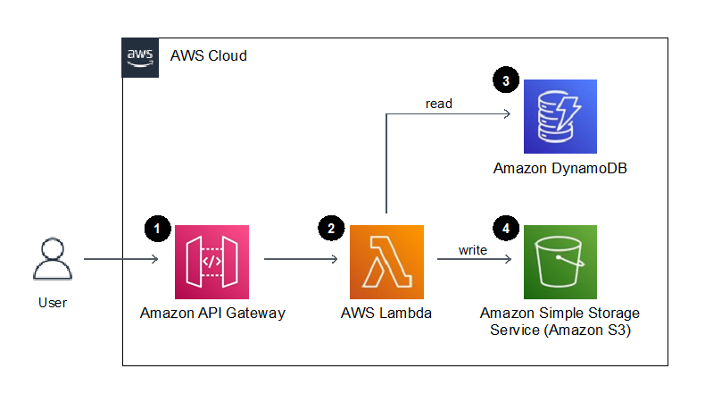
Figure 1. Example application architecture
- Amazon API Gateway provides an endpoint to request the generation of a document for a given customer. A document type and customer identifier are provided in this API call.
- The endpoint invokes an AWS Lambda function that generates a document using the customer identifier and the document type provided.
- An Amazon DynamoDB table stores the contents of the documents and the users name, which are retrieved by the Lambda function.
- The resulting text document is stored to Amazon S3.
Our testing goal is to determine if an isolated “unit” of code works as intended. In this blog, we will be writing tests to provide confidence that the logic written in the above AWS Lambda function behaves as we expect. We will mock the service integrations to Amazon DynamoDB and S3 to isolate and focus our tests on the Lambda function code, and not on the behavior of the AWS Services.
Define the AWS Service resources in the Lambda function
Before writing our first unit test, let’s look at the Lambda function that contains the behavior we wish to test. The full code for the Lambda function is available in the GitHub repository as src/sample_lambda/app.py.
As part of our Best practices for working AWS Lambda functions, we recommend initializing AWS service resource connections outside of the handler function and in the global scope. Additionally, we can retrieve any relevant environment variables in the global scope so that subsequent invocations of the Lambda function do not repeatedly need to retrieve them. For organization, we can put the resource and variables in a dictionary:
_LAMBDA_DYNAMODB_RESOURCE = { "resource" : resource('dynamodb'),
                              "table_name" : environ.get("DYNAMODB_TABLE_NAME","NONE") }
However, globally scoped code and global variables are challenging to test in Python, as global statements are executed on import, and outside of the controlled test flow. To facilitate testing, we define classes for supporting AWS resource connections that we can override (patch) during testing. These classes will accept a dictionary containing the boto3 resource and relevant environment variables.
For example, we create a DynamoDB resource class with a parameter “boto3_dynamodb_resource” that accepts a boto3 resource connected to DynamoDB:
class LambdaDynamoDBClass:
    def __init__(self, lambda_dynamodb_resource):
        self.resource = lambda_dynamodb_resource["resource"]
        self.table_name = lambda_dynamodb_resource["table_name"]
        self.table = self.resource.Table(self.table_name)
Build the Lambda Handler
The Lambda function handler is the method in the AWS Lambda function code that processes events. When the function is invoked, Lambda runs the handler method. When the handler exits or returns a response, it becomes available to process another event.
To facilitate unit test of the handler function, move as much of logic as possible to other functions that are then called by the Lambda hander entry point. Also, pass the AWS resource global variables to these subsequent function calls. This approach enables us to mock and intercept all resources and calls during test.
In our example, the handler references the global variables, and instantiates the resource classes to setup the connections to specific AWS resources. (We will be able to override and mock these connections during unit test.)
Then the handler calls the create_letter_in_s3 function to perform the steps of creating the document, passing the resource classes. This downstream function avoids directly referencing the global context or any AWS resource connections directly.
def lambda_handler(event: APIGatewayProxyEvent, context: LambdaContext) -> Dict[str, Any]:

    global _LAMBDA_DYNAMODB_RESOURCE
    global _LAMBDA_S3_RESOURCE

    dynamodb_resource_class = LambdaDynamoDBClass(_LAMBDA_DYNAMODB_RESOURCE)
    s3_resource_class = LambdaS3Class(_LAMBDA_S3_RESOURCE)

    return create_letter_in_s3(
            dynamo_db = dynamodb_resource_class,
            s3 = s3_resource_class,
            doc_type = event["pathParameters"]["docType"],
            cust_id = event["pathParameters"]["customerId"])
Unit testing with mock AWS services
Our Lambda function code has now been written and is ready to be tested, let’s take a look at the unit test code! The full code for the unit test is available in the GitHub repository as tests/unit/src/test_sample_lambda.py.
In production, our Lambda function code will directly access the AWS resources we defined in our function handler; however, in our unit tests we want to isolate our code and replace the AWS resources with simulations. This isolation facilitates running unit tests in an isolated environment to prevent accidental access to actual cloud resources.
Moto is a python library for Mocking AWS Services that we will be using to simulate AWS resource our tests. Moto supports many AWS resources, and it allows you to test your code with little or no modification by emulating functionality of these services.
Moto uses decorators to intercept and simulate responses to and from AWS resources. By adding a decorator for a given AWS service, subsequent calls from the module to that service will be re-directed to the mock.
@moto.mock_dynamodb
@moto.mock_s3
Configure Test Setup and Tear-down
The mocked AWS resources will be used during the unit test suite. Using the setUp() method allows you to define and configure the mocked global AWS Resources before the tests are run.
We define the test class and a setUp() method and initialize the mock AWS resource. This includes configuring the resource to prepare it for testing, such as defining a mock DynamoDB table or creating a mock S3 Bucket.
class TestSampleLambda(TestCase):
    def setUp(self) -> None:
        dynamodb = boto3.resource("dynamodb", region_name="us-east-1")
        dynamodb.create_table(
            TableName = self.test_ddb_table_name,
            KeySchema = [{"AttributeName": "PK", "KeyType": "HASH"}],
            AttributeDefinitions = [{"AttributeName": "PK",
                                     "AttributeType": "S"}],
            BillingMode = 'PAY_PER_REQUEST'

        s3_client = boto3.client('s3', region_name="us-east-1")
        s3_client.create_bucket(Bucket = self.test_s3_bucket_name )
After creating the mocked resources, the setup function creates resource class object referencing those mocked resources, which will be used during testing.
        mocked_dynamodb_resource = resource("dynamodb")
        mocked_s3_resource = resource("s3")
        mocked_dynamodb_resource = { "resource" : resource('dynamodb'),
                                     "table_name" : self.test_ddb_table_name  }
        mocked_s3_resource = { "resource" : resource('s3'),
                               "bucket_name" : self.test_s3_bucket_name }
        self.mocked_dynamodb_class = LambdaDynamoDBClass(mocked_dynamodb_resource)
        self.mocked_s3_class = LambdaS3Class(mocked_s3_resource)
Test #1: Verify the code writes the document to S3
Our first test will validate our Lambda function writes the customer letter to an S3 bucket in the correct manner. We will follow the standard test format of arrange, act, assert when writing this unit test.
Arrange the data we need in the DynamoDB table:
def test_create_letter_in_s3(self) -> None:

    self.mocked_dynamodb_class.table.put_item(Item={"PK":"D#UnitTestDoc",
                                                        "data":"Unit Test Doc Corpi"})
    self.mocked_dynamodb_class.table.put_item(Item={"PK":"C#UnitTestCust",
                                                        "data":"Unit Test Customer"})
Act by calling the create_letter_in_s3 function. During these act calls, the test passes the AWS resources as created in the setUp().
    test_return_value = create_letter_in_s3(
                        dynamo_db = self.mocked_dynamodb_class,
                        s3=self.mocked_s3_class,
                        doc_type = "UnitTestDoc",
                        cust_id = "UnitTestCust"
                        )
Assert by reading the data written to the mock S3 bucket, and testing conformity to what we are expecting:
bucket_key = "UnitTestCust/UnitTestDoc.txt"
    body = self.mocked_s3_class.bucket.Object(bucket_key).get()['Body'].read()

    self.assertEqual(test_return_value["statusCode"], 200)
    self.assertIn("UnitTestCust/UnitTestDoc.txt", test_return_value["body"])
    self.assertEqual(body.decode('ascii'),"Dear Unit Test Customer;\nUnit Test Doc Corpi")
Tests #2 and #3: Data not found error conditions
We can also test error conditions and handling, such as keys not found in the database. For example, if a customer identifier is submitted, but does not exist in the database lookup, does the logic handle this and return a “Not Found” code of 404?
To test this in test #2, we add data to the mocked DynamoDB table, but then submit a customer identifier that is not in the database.
This test, and a similar test #3 for “Document Types not found”, are implemented in the example test code on GitHub.
Test #4: Validate the handler interface
As the application logic resides in independently tested functions, the Lambda handler function provides only interface validation and function call orchestration. Therefore, the test for the handler validates that the event is parsed correctly, any functions are invoked as expected, and the return value is passed back.
To emulate the global resource variables and other functions, patch both the global resource classes and logic functions.
    @patch("src.sample_lambda.app.LambdaDynamoDBClass")
    @patch("src.sample_lambda.app.LambdaS3Class")
    @patch("src.sample_lambda.app.create_letter_in_s3")
    def test_lambda_handler_valid_event_returns_200(self,
                            patch_create_letter_in_s3 : MagicMock,
                            patch_lambda_s3_class : MagicMock,
                            patch_lambda_dynamodb_class : MagicMock
                            ):
Arrange for the test by setting return values for the patched objects.
patch_lambda_dynamodb_class.return_value = self.mocked_dynamodb_class
        patch_lambda_s3_class.return_value = self.mocked_s3_class

        return_value_200 = {"statusCode" : 200, "body":"OK"}
        patch_create_letter_in_s3.return_value = return_value_200
We need to provide event data when invoking the Lambda handler. A good practice is to save test events as separate JSON files, rather than placing them inline as code. In the example project, test events are located in the folder “tests/events/”. During test execution, the event object is created from the JSON file using the utility function named load_sample_event_from_file.
Act by calling the lambda_handler function.
test_return_value = lambda_handler(event=test_event, context=None)Assert by ensuring the create_letter_in_s3 function is called with the expected parameters based on the event, and a create_letter_in_s3 function return value is passed back to the caller. In our example, this value is simply passed with no alterations.
patch_create_letter_in_s3.assert_called_once_with(
                                        dynamo_db=self.mocked_dynamodb_class,
                                        s3=self.mocked_s3_class,
                                        doc_type=test_event["pathParameters"]["docType"],
                                        cust_id=test_event["pathParameters"]["customerId"])

       self.assertEqual(test_return_value, return_value_200)
Tear Down
The tearDown() method is called immediately after the test method has been run and the result is recorded. In our example tearDown() method, we clean up any data or state created so the next test won’t be impacted.
Running the unit tests
The unittest Unit testing framework can be run using the Python pytest utility. To ensure network isolation and verify the unit tests are not accidently connecting to AWS resources, the pytest-socket project provides the ability to disable network communication during a test.
The pytest command results in a PASSED or FAILED status for each test. A PASSED status verifies that your unit tests, as written, did not encounter errors or issues,
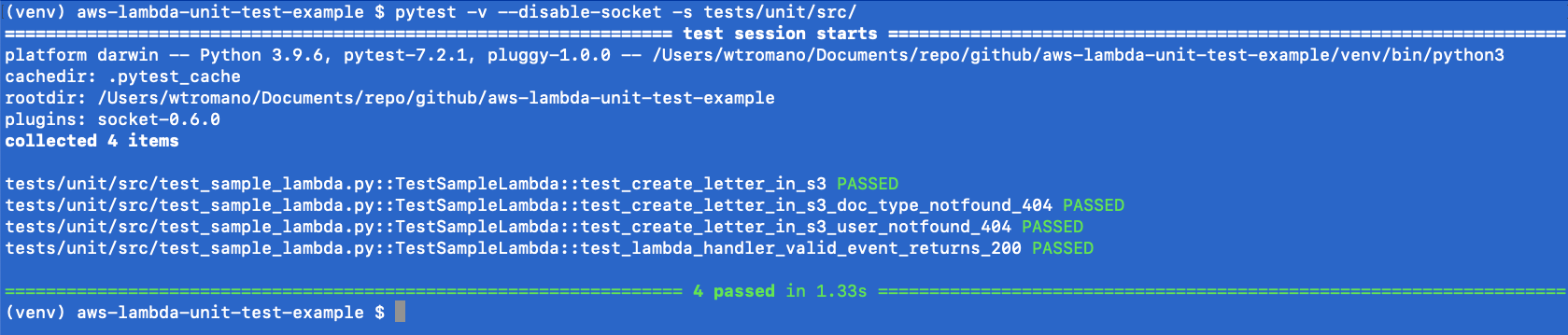
Conclusion
Unit testing is a software development process in which different parts of an application, called units, are individually and independently tested. Tests validate the quality of the code and confirm that it functions as expected. Other developers can gain familiarity with your code base by consulting the tests. Unit tests reduce future refactoring time, help engineers get up to speed on your code base more quickly, and provide confidence in the expected behaviour.
We’ve seen in this blog how to unit test AWS Lambda functions and mock AWS Services to isolate and test individual logic within our code.
AWS Lambda Powertools for Python has been used in the project to validate hander events. Powertools provide a suite of utilities for AWS Lambda functions to ease adopting best practices such as tracing, structured logging, custom metrics, idempotency, batching, and more.
Learn more about AWS Lambda testing in our prescriptive test guidance, and find additional test examples on GitHub. For more serverless learning resources, visit Serverless Land.
About the authors: