Amazon OpenSearch Service launches a modernized operational analytics experience that can provide comprehensive observability spanning multiple data sources, so that you can gain insights from OpenSearch and other integrated data sources in one place. The launch also introduces OpenSearch Workspaces that provides tailored experience for popular use cases and supports access control, so that you can create a private space for your use case and share it only to your collaborators. With the next-generation user interface (UI), the Discover experience has been improved to simplify interactive analysis, so that you can easily utilize features such as natural language query generation to gain insights from your data.
Multiple Data Source: You might have already used OpenSearch Dashboards to provide an operational analytics experience for your OpenSearch clusters. OpenSearch Dashboards is co-located with a cluster, so that each OpenSearch Dashboards can only work with one cluster. And as you scale up your workload across multiple clusters, there is not a unified experience to analyze your data in one place. In comparison, the next-generation OpenSearch UI is designed to work across multiple OpenSearch clusters to aggregate the comprehensive insights in one place. An OpenSearch application is an instance of the next-generation OpenSearch UI. Currently, OpenSearch applications can be associated with multiple OpenSearch clusters (above version 1.3), Amazon OpenSearch Service Serverless collections, and integrated data sources such as Amazon S3. Each OpenSearch cluster can be associated with multiple OpenSearch applications, in addition to its co-located OpenSearch Dashboards that will remain functional.
Workspace: With workspaces, you can easily create your use case specific contents in a private space and manage the permissions in team collaboration. Workspace provide curated experiences for popular use cases such as Observability, Security Analytics and Search, so that you can find it straightforward to build contents for your use case. Workspace supports collaborator management, so that you can share your workspace only to your intended collaborators, and manage the permissions for each collaborator.
Discover: The improved Discover feature now provides a unified log exploration experience that adds the support for SQL and Piped Processing Language (PPL), in addition to the existing support for DQL and Lucene. Discover features a new data selector to support multiple data sources, a new visual design, query autocomplete and natural language query generation for improved usability. With the enhanced Discover interface, you can now analyze data from multiple sources without switching tools, reducing complexity and improving efficiency.
Solution Overview
The following diagram illustrates architecture of the OpenSearch Dashboards.
The following diagram illustrates the next-generation OpenSearch UI architecture.
In the following sections, we discuss the following topics
The process of creating an application
Setting up and using the new Workspaces functionality
The enhanced Discover experience
We’ll demonstrate how these improvements streamline data analysis, foster collaboration, and empower you to extract insights more efficiently across various use cases.
Create an application:
To begin using the next-generation OpenSearch UI, you can first create an application. An application is an instance of the OpenSearch UI (Dashboards), and you have the flexibility to create multiple applications within a single account. To create a new application, complete the following steps:
On the Amazon OpenSearch Service console, choose OpenSearch UI (Dashboards)under Central management in the navigation panel.
Choose Create application.
For application name, enter a descriptive name for your new application.
AWS Identity and Access Management (IAM) is the default authentication mechanism. Optionally, you can select Authentication with IAM Identity Center (IDC), so that you can use credentials and access management from your existing identity providers to manage user access.
For OpenSearch application admins, specify the IAM principals or IDC users that will have permissions to update or delete the application configuration. You will automatically be set as the first admin.
This page lists all the existing applications under your account in the current AWS region. You can create new application from this page.
This page is the create application workflow. You can specify the application name, enable/disable IDC and define application admins to create an application.
After you configured these settings and created an application, your new OpenSearch application will be ready for you to associate data sources and start using the enhanced UI capabilities.
Associating data sources:
After you create your new OpenSearch application, the next step is to associate the relevant data sources. This allows you to connect the application to the necessary OpenSearch domains, collections, and other data sources.
On the application details page, choose Manage data sources.
You will be presented with a list of all the OpenSearch data sources you have access to, including managed domains and serverless collections.
Select the data sources you want to associate with this application.
OpenSearch domains below version v1.3 will not be compatible with the next-generation UI, and will be grayed out in the list. Additionally, if you need to connect to a domain within a virtual private cloud (VPC), you will need to authorize OpenSearch application as a new principal under its security configurations. If you need to connect to a collection within a VPC, you will need to configure its network policy to Private, enable AWS service private access with OpenSearch application.
Choose Save to finalize the data source association.
Your OpenSearch application is now ready to use, with access to the connected data.
Working with the OpenSearch application:
To access your new OpenSearch application, you can either choose the application URL or choose Launch application on the application details page. After you’ve successfully logged in either with IAM or IDC, you’ll be directed to the application’s homepage. From here, you can choose to create a new workspace or navigate to an existing one that you have access to.
Creating a new workspace:
A workspace is a tailored experience for your use case and team collaboration. There are five types of workspaces: Observability, Security Analytics, Search, Essentials, and Analytics. You can click on the info button to learn more about each workspace type. Existing workspaces will be listed on the homepage. To create a new workspace, complete the following steps:
Choose Create workspace.
Enter a name for your workspace.
Optionally, you can select a different color for the workspace icon for easier identification.
Select the type of workspace you want to create: Observability, Security Analytics, Search, Essentials, or Analytics
Add at least one data source for this workspace (from the list of data sources you previously associated with the application).
For this post, we create an Observability workspace named MyWorkspace and associate it with one Amazon OpenSearch Serverless collection and one Amazon OpenSearch Service managed cluster. You can always manage the data sources associated with a workspace, even after it has been created.
Invite Collaborators
After you create your new workspace, you can add users or groups as collaborators. Workspace collaborators are the users you want to invite to work with you in this workspace, and there are three available permission levels for collaborators: admin, read/write, and read-only. Read/write permission allows a collaborator to create, edit and delete the dashboards, visualizations, and saved queries within the workspace, whereas collaborators with read-only access can only view the results. Admin level gives a collaborator the same permissions as you to not only read/write but also update the configurations of the workspace or delete it.
To add collaborators to your workspace, complete the following steps:
Choose Collaborators in the navigation panel.
Choose Add collaborators.
Choose the type of users you want to add as collaborators. You can add collaborators by their IAM Amazon Resource Name (ARN) or IDC username.
Select a permission level for the collaborator from the three options: Read only, Read and write, and Admin
If you do not know the ARN of your intended collaborator, follow the instruction to check for their ARN, for example.
Improved navigation:
The improved navigation in workspaces provides a more contextual and purpose-built interface, ensuring that each workspace includes only the tools and features relevant to its use case. With enhanced clarity and better organization, the new navigation system is tailored to help you find the features you need quickly, improving overall productivity and minimizing time spent searching through menus.
Revamped Discover experience
Discover is now revamped to offer improved usability and efficiency. You can access multiple data sources, natural language query generation, a new data selector, and polished design with optimized data density, allowing you to effortlessly navigate and analyze your data:
Unified language selector – Discover now offers a unified language selector, allowing users to choose from SQL, PPL, Dashboards Query Language (DQL), or Lucene, making it convenient to work with your preferred query languages in one place.
Natural language query generation – Discover now supports natural language query building for PPL. Enter your questions in plain language, and Discover converts them to PPL syntax, making data exploration simpler and more accessible. This new feature empowers users of different skill levels to get insights without needing to fully understand the PPL syntax.
Powerful query autocomplete – The enhanced query bar includes autocomplete functionality and natural language query generation support, simplifying query building by offering relevant suggestions as you type, making it faster and more efficient to write complex queries
New data selector– The new data selector makes it straightforward to connect to multiple data sources, bringing data from Amazon OpenSearch Service domains and serverless collections, and Amazon S3 into a unified view.
Conclusion
In this post, we discussed the features of the next-generation OpenSearch UI. These improvements streamline data analytics, foster collaboration, and empower you to extract insights more efficiently across various use cases.
You can create your own OpenSearch UI applications today in the US East (N. Virginia), US West (N. California, Oregon), Asia Pacific (Mumbai, Singapore, Sydney, Tokyo), South America (São Paulo), Europe (Frankfurt, Ireland, London, Paris) and Canada (Central) Regions.
About the Authors
Hang (Arthur) Zuo is a Senior Product Manager with Amazon OpenSearch Service. Arthur leads the core experience in the next-gen OpenSearch UI and data migration to Amazon OpenSearch Service. Arthur is passionate about cloud technologies and building data products that help users and businesses gain actionable insights and achieve operational excellence.
Rushabh Vora is a Principal Product Manager for the OpenSearch project of Amazon Web Services. Rushabh leads core experiences in data exploration, dashboards, visualizations, reporting, and data management to help organizations unlock insights at scale. Rushabh is passionate about cloud technologies and building products that enable businesses to make data-driven decisions and achieve operational excellence.
Sohaib Katariwala is a Senior Specialist Solutions Architect at AWS focused on Amazon OpenSearch Service based out of Chicago, IL. His interests are in all things data and analytics. More specifically he loves to help customers use AI in their data strategy to solve modern day challenges.
Arun Lakshmanan is a Search Specialist with Amazon OpenSearch Service based out of Chicago, IL. He works closely with customers on their OpenSearch journey across various use cases including vector search, observability, and security analytics.
Xenia Tupitsyna is a UX Designer at OpenSearch. She is working on user experiences across security analytics solutions, anomaly detection, alerting, and core dashboards.
Flexible arrays — arrays that are declared as the final member of a
structure and which have a size determined at run time — have long drawn
the attention of developers seeking to harden the kernel against
buffer-overflow vulnerabilities. These arrays have reliably been a source
of bugs, so anything that can be done to ensure that operations on them
stay within bounds is a welcome improvement. While many improvements,
including the recent counted-by work, have
been made, one of the most difficult cases remains. Now, however,
developers who are interested in using recent compiler bounds-checking
features are trying to get a handle on struct sockaddr.
Accelerating SQL code migration from Google BigQuery to Amazon Redshift can be a complex and time-consuming task. Businesses often struggle to efficiently translate their existing BigQuery code to Amazon Redshift, which can delay critical data modernization initiatives. However, with the right tools and approach, this migration process can be significantly streamlined.
This post explores how you can use BladeBridge, a leading data environment modernization solution, to simplify and accelerate the migration of SQL code from BigQuery to Amazon Redshift. BladeBridge offers a comprehensive suite of tools that automate much of the complex conversion work, allowing organizations to quickly and reliably transition their data analytics capabilities to the scalable Amazon Redshift data warehouse. BladeBridge provides a configurable framework to seamlessly convert legacy metadata and code into more modern services such as Amazon Redshift.
Amazon Redshift is a fully managed data warehouse service offered by Amazon Web Services (AWS). Tens of thousands of customers use Amazon Redshift every day to run analytics, processing exabytes of data for business insights. Whether your growing data is stored in operational data stores, data lakes, streaming data services, or third-party datasets, Amazon Redshift helps you securely access, combine, and share data with minimal movement or copying. Amazon Redshift is built for scale and delivers up to 7.9 times better price performance than other cloud data warehouses.
By using the BladeBridge Analyzer and BladeBridge Converter tools, organizations can significantly reduce the time and effort required to migrate BigQuery code to Amazon Redshift. The Analyzer provides detailed assessments of the complexity and requirements for the migration, and the Converter automates the actual code conversion process, using pattern-based customizable rules to streamline the transition.
In this post, we walk through the step-by-step process of using BladeBridge to accelerate the migration of BigQuery SQL code to Amazon Redshift.
Solution overview
The BladeBridge solution is composed of two key components: the BladeBridge Analyzer and the BladeBridge Converter.
BladeBridge Analyzer
The Analyzer is designed to thoroughly assess the complexities of the existing data environment, in this case, Google BigQuery. After assessment of the source SQL files, it generates a comprehensive report that provides valuable insights into the migration effort. The Analyzer report includes the following:
Summary of the total number of SQL scripts, file scripts, data definition language (DDL) statements, and other key metrics
Categorization of the SQL code complexity into levels such as low, medium, complex, and very complex
Insights that help both the organizations and systems integrators prepare more accurate project estimates and migration plans
BladeBridge Converter
The Converter is a pattern-based automation tool that streamlines the actual code conversion process from BigQuery to Amazon Redshift. The Converter uses a set of predefined conversion rules and patterns to automatically translate 70–95% of the legacy SQL code. This significantly reduces the manual effort required by developers. The Converter works by doing the following:
Parsing the source SQL files and analyzing the code semantically
Applying the appropriate translation rules and patterns to convert source database code to the target, in this case, Google BigQuery to Amazon Redshift
The out-of-the-box code handles most conversions. The Converter allows developers to customize the conversion patterns for more complex transformations.
An Amazon Elastic Compute Cloud (Amazon EC2) instance, on-premises server, or desktop or laptop with the following requirements:
MacOS, Windows 7 or higher with 32-bit or 64-bit, Linux Redhat, Ubuntu, or similar operating system
A minimum of 8 GB RAM is recommended
Visit the BladeBridge community portal and sign up to create your account. The portal gives you access to a comprehensive suite of resources, including the BladeBridge Analyzer, Converter, and other training materials. This post contains some links that are only accessible to registered members of the BladeBridge community portal.
Contact BladeBridge through Request demo and obtain an Analyzer key for your organization.
Solution walkthrough
Follow these solution steps:
Prepare SQL files
For SQL data warehouses such as BigQuery, code preparation starts by exporting the SQL files out of the data warehouse solution. If your BigQuery SQL code is stored in a single file containing multiple database objects, you need to split them into individual files before using the BladeBridge tools to convert the code to Amazon Redshift. To split into multiple files, you can use the BladeBridge SQL File Splitter utility. The BladeBridge conversion process is optimized to work with each database object (for example, tables, views, and materialized views) and code object (for example, stored procedures and functions) stored in its own separate SQL file. This allows the BladeBridge Analyzer to scan each file individually, gaining a comprehensive understanding of the code patterns, complexity, and structure. To use BladeBridge SQL File Splitter utility, follow these steps:
Create an input file directory and place your BigQuery SQL code files in the directory.
Create an empty output file directory. The files generated by the splitter will be stored here.
Navigate to the directory where you downloaded the bbsqlsplit executable file and run the following command in your terminal (Mac or Linux) or command prompt (Windows), replacing the input and output file directory paths:
For more options of the bbsqlsplit command, refer to the SQL file split documentation in the BladeBridge community portal.
Using BladeBridge Analyzer, create an analyzer report
The Analyzer provides a detailed assessment of the existing BigQuery code, generating a comprehensive report that outlines the complexity and requirements for the migration to Amazon Redshift.
To run the BladeBridge Analyzer, follow these steps:
Log in to the BladeBridge portal and navigate to the Analyzer Download
Download the Analyzer executable file for your operating system (for example, bbanalyzer.exe for Windows, bbanalyzer.gz for Linux and macOS). For macOS and Linux users, you need to deflate the downloaded gzip file.
Download the configuration file (general_sql_specs.json) from the BladeBridge community portal, as shown in the following screenshot.
On the BladeBridge community portal, choose Assets. This page should display the Analyzer key for your organization.
From the assets page, download the Analyzer key as shown in the following screenshot.
In the directory where you downloaded the bbanalyzer executable file, run the following command in your terminal (Mac or Linux) or command prompt (Windows), replacing the necessary paths.
Syntax
bbanalyzer

######## OPTIONS ########

-c <<path to your analyzer key>>

-t SQL

-d <<path to your source code directory>>

-r <<name for the output report>>.xlsx
After running the command successfully, the Analyzer generates a report. Review the report thoroughly, because it provides a summary and in-depth explanations of the SQL analysis. The summary sheet, shown in the following image, provides an overview of the migration, including the number of total SQL scripts, file scripts, and DDLs. Each SQL script is categorized into LOW, MEDIUM, COMPLEX, or VERY_COMPLEX complexities, which are determined by the Analyzer Complexity Determination Algorithm. The summary will also help with understanding the overall complexity and migration effort before performing the actual conversion.
If you observe an error when running BladeBridge Analyzer, review following troubleshooting tips:
Configure the write permission – You may need to add necessary permission to the analyzer executable file. For Mac and Linux users, run chmod 755 ./bbanalyzer to modify the permission.
Allow running third party software – Because BladeBridge Analyzer is a third-party software, MacOS may raise a warning or an error when running Analyzer. If you’re using Mac, follow the instructions in Open a Mac app from an unidentified developer.
Use local drive – In some cases, you might encounter an error if the executable is located in a network drive. We recommend that you run the executable on the local drive.
Don’t include whitespace in the path – Make sure the path to the executable doesn’t contain a directory with spaces in the directory name.
To use the BladeBridge Converter and automate the code translation process, you need to purchase the necessary license keys. These license keys are tied to the specific SQL files you are converting, making sure that updates to the source code require the appropriate license.
The BladeBridge team will review the information and provide you with the required license keys to run the Converter.
The license key is tied to the file hash of the SQL files you are converting. If you make updates to the source SQL files, you need to purchase new license keys to convert the modified code. Therefore, make sure to purchase the necessary license keys and manage your files with a version control system to have smooth transitions when converting your BigQuery SQL code to Amazon Redshift.
Using BladeBridge Converter, convert SQL files
The Converter uses the predefined conversion rules that are available in the out-of-the-box configuration files to automatically translate 70–95% of the legacy code, significantly reducing manual effort for your development team. The out-of-the-box configuration file handles conversion for common code patterns from Google BigQuery to Amazon Redshift. For those custom patterns that aren’t covered by an out-of-the-box configuration file, you can create custom conversion rules by creating additional configuration files.
Follow these steps to run the BladeBridge Converter:
Log in to the BladeBridge portal and on the Convertor downloads page, download the Convertor executable file for your operating system (sqlconv.exe for Windows or sqlconv.gz for Mac or Linux)
From the same page, download the configuration file (general_sql_specs.json)
Create an output directory where the converted files will be saved
In the folder where you downloaded the Convertor executable sqlconv, run the following command
Syntax
sqlconv

-c <<converter license file name obtained from BladeBridge>>

-d <<input folder for SQL files>>

-n <<output folder for converted files>>

-u <<path for the config files/s provide at least one file>>
Run the generated SQL files in your Amazon Redshift data warehouse. If you encounter errors, analyze them and determine if custom conversion rules, not already covered in the out-of-the-box configuration files, need to be applied.
If custom conversion rules are needed, create a new configuration file following the guidelines in the Customize Configuration File section. Provide the new config file name in the -u option and rerun the Converter.
Repeat these steps until all files are converted successfully or manually modified.
Customize configuration file
Customizing a configuration file is an iterative process that can help automate the conversion for occurrences in your codebase. However, manual conversion may be required if the conversion is needed for only a few files and a few occurrences.
The configuration is defined in a JSON file. There is a general configuration file with common rules and custom configuration files for each client with client-specific rules. Rules can be added to the general configuration file if they are applicable for all clients. For client-specific rules, a separate JSON file should be created and referenced. This keeps the general rules clean and organized.
The conversion rules in BladeBridge’s configuration file fall into one of three categories:
Every line ending with a ; is a statement. This line ending also can be replaced with other breakers. Refer to this BladeBridge documentation to get more details on SQL and expression conversion.
The following are considerations while using the customized configuration:
Nested functions in BigQuery allow for complex operations within a single SQL statement, which may need to be broken down into multiple steps in Amazon Redshift
Array functions in BigQuery provide capabilities for manipulating and transforming array data types, which may require alternative approaches in Amazon Redshift
You need to carefully analyze the requirements and implement workarounds or alternative solutions when migrating from BigQuery to Amazon Redshift, especially for advanced functionality not directly supported in Amazon Redshift
Line substitution
Line substitution applies regular expressions to each line of code. This has the from clause, which has the expression to be converted. The to section has the target mapping for which it’ll be converted. Statement_categories limit the application of line substitution to specific statements such as DDL or procedure. For example:
The first expression in the following code example replaces the regular expression pattern ROWNUM with the SQL expression row_number() over (order by 1)
The second expression in the following code example replaces the regular expression pattern SYSDATE with the SQL expression CURRENT_TIMESTAMP.
“line_subst” : [
{“from” : “\bROWNUM\b”, “to” : “row_number() over (order by 1)”},
{“from” : “SYSDATE”, “to” : “CURRENT_TIMESTAMP”}
]
Block substitution
Block substitution applies regular expressions across multiple lines. This applies to statements that stretch over multiple lines, which are generally more complex than the line substitutions. The following expression in the example replaces the block. In this example, the procedure is created in the target database.
BEGIN

EXECUTE IMMEDIATE(‘SQL Statement’);

EXCEPTION WHEN OTHERS

THEN

NULL

END;

To

CALL SP_DYN_SQL(‘parameters’);

“block_subst” : [
{“from”: “BEGIN(.*?)execute immediate(.*);.*exception\s*when\s*others\s*then\s*null(.*?)end;(.*)”, “to”: “CALL sp_dyn_sql($2);”}
]
Function substitution
Function substitution allows replacing one function with an equivalent function in the target data warehouse. The configuration also allows for specifying custom functions.
Function substitution points to an array of instructions responsible for altering function calls. This section is used when function translations are required or function arguments (function signature) have to be altered. The following expression converts the NVL2 function to CASE function on Amazon Redshift.
“function_subst” : [
{“from”: “NVL2”, “output_template” : “CASE WHEN $1 IS NOT NULL THEN $2 ELSE $3 END”}
]
Conclusion
In this post, we demonstrated how to use the BladeBridge Analyzer and BladeBridge Converter to streamline the migration of SQL code from Google BigQuery to Amazon Redshift. By using BladeBridge, organizations can significantly reduce the time and effort required to translate their existing BigQuery code for migration to the Amazon Redshift data warehouse. The Analyzer provides a detailed assessment of the source SQL code, and the Converter automates the actual conversion process using a set of predefined, customizable rules and patterns.
We also covered the customization capabilities of the BladeBridge solution, showcasing how you can tailor the conversion rules to handle more complex transformations. By using the line substitution, block substitution, and function substitution features, you can have a seamless migration that addresses the unique requirements of your data analytics infrastructure.
We encourage you to try out BladeBridge’s GCP BigQuery to Amazon Redshift solution and explore the various configuration options. If you encounter any challenges or have additional requirements, refer to the BladeBridge community support portal or reach out to the BladeBridge team for further assistance.
About the authors
Ritesh Kumar Sinha is an Analytics Specialist Solutions Architect based out of San Francisco. He has helped customers build scalable data warehousing and big data solutions for over 16 years. He loves to design and build efficient end-to-end solutions on AWS. In his spare time, he loves reading, walking, and doing yoga.
Anusha Challa is a Senior Analytics Specialist Solutions Architect focused on Amazon Redshift. She has helped many customers build large-scale data warehouse solutions in the cloud and on premises. She is passionate about data analytics and data science.
Yota Hamaoka is an Analytics Solution Architect at Amazon Web Services. He is focused on driving customers to accelerate their analytics journey with Amazon Redshift.
Milind Oke is a Data Warehouse Specialist Solutions Architect based out of New York. He has been building data warehouse solutions for over 15 years and specializes in Amazon Redshift.
Raza Hafeez is a Senior Product Manager at Amazon Redshift. He has over 13 years of professional experience building and optimizing enterprise data warehouses and is passionate about enabling customers to realize the power of their data. He specializes in migrating enterprise data warehouses to AWS Modern Data Architecture.
Large language models (LLMs) are increasingly being harnessed to automate cyberattacks, making sophisticated exploits more accessible and scalable. In response, we propose a new defense strategy tailored to counter LLM-driven cyberattacks. We introduce Mantis, a defensive framework that exploits LLMs’ susceptibility to adversarial inputs to undermine malicious operations. Upon detecting an automated cyberattack, Mantis plants carefully crafted inputs into system responses, leading the attacker’s LLM to disrupt their own operations (passive defense) or even compromise the attacker’s machine (active defense). By deploying purposefully vulnerable decoy services to attract the attacker and using dynamic prompt injections for the attacker’s LLM, Mantis can autonomously hack back the attacker. In our experiments, Mantis consistently achieved over 95% effectiveness against automated LLM-driven attacks. To foster further research and collaboration, Mantis is available as an open-source tool: this https URL.
This isn’t the solution, of course. But this sort of thing could be part of a solution.
On October 24, 2024, the National Institute of Standards and Technology (NIST) announced that they’re advancing fourteen post-quantum signature schemes to the second round of the “signatures on ramp” competition. “Post-quantum” means that these algorithms are designed to resist the attack of quantum computers. NIST already standardized four post-quantum signature schemes (ML-DSA, SLH-DSA, XMSS, and LHS) and they are drafting a standard for a fifth (Falcon). Why do we need even more, you might ask? We’ll get to that.
A regular reader of the blog will know that this is not the first time we’ve taken measure of post-quantum signatures. In 2021 we took a first hard look, and reported on the performance impact we expect from large-scale measurements. Since then, dozens of new post-quantum algorithms have been proposed. Many of them have been submitted to this new NIST competition. We discussed some of the more promising ones in our early 2024 blog post.
In this blog post, we will go over the fourteen schemes advanced to the second round of the on ramp and discuss their feasibility for use in TLS — the protocol that secures browsing the Internet. The defining feature of practically all of them, is that they require much more bytes on the wire. Back in 2021 we shared experimental results on the impact of these extra bytes. Today, we will share some surprising statistics on how TLS is used in practice. One is that today already almost half the data sent over more than half the QUIC connections are just for the certificates.
For a broader context and introduction to the post-quantum migration, check out our early 2024 blog post. One take-away to mention here: there will be two migrations for TLS. First, we urgently need to migrate key agreement to post-quantum cryptography to protect against attackers that store encrypted communication today in order to decrypt it in the future when a quantum computer is available. The industry is making good progress here: 18% of human requests to websites using Cloudflare are secured using post-quantum key agreement. The second migration, to post-quantum signatures (certificates), is not as urgent: we will need to have this sorted by the time the quantum computer arrives. However, it will be a bigger challenge.
The signatures in TLS
Before we have a look at the long list of post-quantum signature algorithms and their performance characteristics, let’s go through the signatures involved when browsing the Internet and their particular constraints.
When you visit a website, the browser establishes a TLS connection with the server for that website. The connection starts with a cryptographic handshake. During this handshake, to authenticate the connection, the server signs the transcript so far, and presents the browser with a TLS leaf certificate to prove that it’s allowed to serve the website. This leaf certificate is signed by a certification authority (CA). Typically, it’s not signed by the CA’s root certificate, but by an intermediate CA certificate, which in turn is signed by the root CA, or another intermediate. That’s not all: a leaf certificate has to include at least two signed certificate timestamps (SCTs). These SCTs are signatures created by certificate transparency (CT) logs to attest they’ve been publicly logged. Certificate Transparency is what enables you to look up a certificate on websites such crt.sh and merklemap. In the future three or more SCTs might be required. Finally, servers may also send an OCSP staple to demonstrate a certificate hasn’t been revoked.
Thus, we’re looking at a minimum of five signatures (not counting the OCSP staple) and two public keys transmitted across the network to establish a new TLS connection.
Tailoring
Only the handshake transcript signature is created online; the other signatures are “offline”. That is, they are created ahead of time. For these offline signatures, fast verification is much more important than fast signing. On the other hand, for the handshake signature, we want to minimize the sum of signing and verification time.
Only the public keys of the leaf and intermediate certificates are transmitted on the wire during the handshake, and for those we want to minimize the combined size of the signature and the public key. For the other signatures, the public key is not transmitted during the handshake, and thus a scheme with larger public keys would be tolerable, and preferable if it trades larger public keys for smaller signatures.
The algorithms
Now that we’re up to speed, let’s have a look at the candidates that progressed (marked by 🤔 below), compared to the classical algorithms vulnerable to quantum attack (marked by ❌), and the post-quantum algorithms that are already standardized (✅) or soon will be (📝). Each submission proposes several variants. We list the most relevant variants to TLS from each submission. To explore all variants, check out Thom Wigger’s signatures zoo.
Sizes (bytes)
CPU time (lower is better)
Family
Name variant
Public key
Signature
Signing
Verification
Elliptic curves
Ed25519
❌
32
64
0.15
1.3
Factoring
RSA 2048
❌
272
256
80
0.4
Lattices
ML-DSA 44
✅
1,312
2,420
1 (baseline)
1 (baseline)
Symmetric
SLH-DSA 128s
✅
32
7,856
14,000
40
SLH-DSA 128f
✅
32
17,088
720
110
LMS M4_H20_W8
✅
48
1,112
2.9 ⚠️
8.4
Lattices
Falcon 512
📝
897
666
3 ⚠️
0.7
Codebased
CROSS R-SDP(G)1 small
🤔
38
7,956
20
35
LESS 1s
🤔
97,484
5,120
620
1800
MPC in the head
Mirath Mirith Ia fast
🤔
129
7,877
25
60
MQOM L1-gf251-fast
🤔
59
7,850
35
85
PERK I-fast5
🤔
240
8,030
20
40
RYDE 128F
🤔
86
7,446
15
40
SDitH gf251-L1-hyp
🤔
132
8,496
30
80
VOLE in the head
FAEST EM-128f
🤔
32
5,696
6
18
Lattices
HAWK 512
🤔
1,024
555
0.25
1.2
Isogeny
SQISign I
🤔
64
177
17,000
900
Multivariate
MAYO one
🤔
1,168
321
1.4
1.4
MAYO two
🤔
5,488
180
1.7
0.8
QR-UOV I-(31,165,60,3)
🤔
23,657
157
75
125
SNOVA (24,5,4)
🤔
1,016
248
0.9
1.4
SNOVA (25,8,3)
🤔
2,320
165
0.9
1.8
SNOVA (37,17,2)
🤔
9,842
106
1
1.2
UOV Is-pkc
🤔
66,576
96
0.3
2.3
UOV Ip-pkc
🤔
43,576
128
0.3
0.8
Some notes about the table. It compares selected variants of the submissions progressed to the second round of the NIST PQC signature on ramp with earlier existing traditional and post-quantum schemes at the security level of AES-128. CPU times are taken from the signatures zoo, which collected them from the submission documents and some later advances. CPU performance varies significantly by platform and implementation, and should only be taken as a rough indication. We are early in the competition, and the on-ramp schemes will evolve: some will improve drastically (both in compute and size), whereas others will regress to counter new attacks. Check out the zoo for the latest numbers. We marked Falcon signing with a ⚠️, as Falcon signing is hard to implement in a fast and timing side-channel secure manner. LMS signing has a ⚠️, as secure LMS signing requires keeping a state and the listed signing time assumes a 32MB cache. This will be discussed later on.
These are a lot of algorithms, and we didn’t even list all variants. One thing is clear: none of them perform as well as classical elliptic curve signatures across the board. Let’s start with NIST’s 2022 picks.
ML-DSA, SLH-DSA, and Falcon
The most viable general purpose post-quantum signature scheme standardized today is the lattice-based ML-DSA (FIPS 204), which started its life as Dilithium. It’s light on the CPU and reasonably straightforward to implement. The big downside is that its signatures and public keys are large: 2.4kB and 1.3kB respectively. Here and for the balance of the blog post, we will only consider the variants at the AES-128 security level unless stated otherwise. Adding ML-DSA, adds 14.7kB to the TLS handshake (two 1312-byte public keys plus five 2420-byte signatures).
SLH-DSA (FIPS 205, née SPHINCS+) looks strictly worse, adding 39kB and significant computational overhead for both signing and verification. The advantage of SLH-DSA, being solely based on hashes, is that its security is much better understood than ML-DSA. The lowest security level of SLH-DSA is generally more trusted than the highest security levels of many other schemes.
Falcon (to be renamed FN-DSA) seems much better than SLH-DSA and ML-DSA if you look only at the numbers in the table. There is a catch though. For fast signing, Falcon requires fast floating-point arithmetic, which turns out to be difficult to implement securely. Signing can be performed securely with emulated floating-point arithmetic, but that makes it roughly twenty times slower. This makes Falcon ill-suited for online signatures. Furthermore, the signing procedure of Falcon is complicated to implement. On the other hand, Falcon verification is simple and doesn’t require floating-point arithmetic.
Leaning into Falcon’s strength, by using ML-DSA for the handshake signature, and Falcon for the rest, we’re only adding 7.3kB (at security level of AES-128).
There is one more difficulty with Falcon worth mentioning: it’s missing a middle security level. That means that if Falcon-512 (which we considered so far) turns out to be weaker than expected, then the next one up is Falcon-1024, which has double signature and public key size. That amounts to adding about 11kB.
Stateful hash-based signatures
The very first post-quantum signature algorithms standardized are the stateful hash-based XMSS(MT) and LMS/HSS. These are hash-based signatures, similar to SLH-DSA, and so we have a lot of trust in their security. They come with a big drawback: when creating a keypair you prepare a finite number of signature slots. For the variant listed in the table, there are about one million slots. Each slot can only be used once. If by accident a slot is used twice, then anyone can (probably) use those two signatures to forge any new signature from that slot and break into the connection the certificate is supposed to protect. Remembering which slots have been used, is the state in stateful hash-based signature. Certificate authorities might be able to keep the state, but for general use, Adam Langley calls keeping the state a huge foot-cannon.
There are more quirks to keep in mind for stateful hash-based signatures. To start, during key generation, each slot needs to be prepared. Preparing each slot takes approximately the same amount of time as verifying a signature. Preparing all million takes a couple of hours on a single core. For intermediate certificates of a popular certificate authority, a million slots are not enough. Indeed, Let’s Encrypt issues more than four million certificates per day. Instead of increasing the number of slots directly, we can use an extra intermediate. This is what XMSSMT and HSS do internally. A final quirk of stateful hash-based signatures is that their security is bottlenecked on non-repudiation: the listed LMS instance has 192 bits of security against forgery, but only 96 bits against the signer themselves creating a single signature that verifies two different messages.
Even when stateful hash-based signatures or Falcon can be used, we are still adding a lot of bytes on the wire. From earlier experiments we know that that will impact performance significantly. We summarize those findings later in this blog post, and share some new data. The short of it: it would be nice to have a post-quantum signature scheme that outperforms Falcon, or at least outperforms ML-DSA and is easier to deploy. This is one of the reasons NIST is running the second competition.
With that in mind, let’s have a look at the candidates.
Structured lattice alternatives
With only performance in mind, it is surprising that half of the candidates do worse than ML-DSA. There is a good reason for it: NIST is worried that we’re putting all our eggs in the structured lattices basket. SLH-DSA is an alternative to lattices today, but it doesn’t perform well enough for many applications. As such, NIST would primarily like to standardize another general purpose signature algorithm that is not based on structured lattices, and that outperforms SLH-DSA. We will briefly touch upon these schemes here.
Code-based
CROSS and LESS are two code-based signature schemes. CROSS is based on a variant of the traditional syndrome decoding problem. Its signatures are about as large as SLH-DSA, but its edge over SLH-DSA is the much better signing times. LESS is based on the novel linear equivalence problem. It only outperforms SLH-DSA on signature size, requiring larger public keys in return. For use in TLS, the high verification times of LESS are especially problematic. Given that LESS is based on a new approach, it will be interesting to see how much it can improve going forward.
Multi-party computation in the head
Five of the submissions (Mirath, MQOM, PERK, RYDE, SDitH) use the Multi-Party Computation in the Head (MPCitH) paradigm.
It has been exciting to see the developments in this field. To explain a bit about it, let’s go back to Picnic. Picnic was an MPCitH submission to the previous NIST PQC competition. In essence, its private key is a random key x, and its public key is the hash H(x). A signature is a zero-knowledge proof demonstrating that the signer knows x. So far, it’s pretty similar in shape to other signature schemes that use zero knowledge proofs. The difference is in how that proof is created. We have to talk about multi-party computation (MPC) first. MPC starts with splitting the key x into shares, using Shamir secret sharing for instance, and giving each party one share. No single party knows the value of x itself, but they can recover it by recombining. The insight of MPC is that these parties (with some communication) can perform arbitrary computation on the data they shared. In particular, they can compute a secret share of H(x). Now, we can use that to make a zero-knowledge proof as follows. The signer simulates all parties in the multi-party protocol to compute and recombine H(x). The signer then reveals part of the intermediate values of the computation using Fiat–Shamir: enough so that none of the parties could have cheated on any of the steps, but not enough that it allows the verifier to figure out x themselves.
For H, Picnic uses LowMC, a block cipher for which it’s easy to do the multi-party computation. The initial submission of Picnic performed poorly compared to SLH-DSA with 32kB signatures. For the second round, Picnic was improved considerably, boasting 12kB signatures. SLH-DSA won out with smaller signatures, and more conservative security assumptions: Picnic relies on LowMC which didn’t receive as much study as the hashes on which SLH-DSA is based.
Back to the MPCitH candidates that progressed. All of them have variants (listed in the table) with similar or better signature sizes as SLH-DSA, while outperforming SLH-DSA considerably in signing time. There are variants with even smaller signatures, but their verification performance is significantly higher. The difference between the MPCitH candidates is the underlying trapdoor they use. In Picnic the trapdoor was LowMC. For both RYDE and SDiTH, the trapdoors used are based on variants of syndrome decoding, and could be classified as code-based cryptography.
Over the years, MPCitH schemes have seen remarkable improvements in performance, and we don’t seem to have reached the end of it yet. There is still some way to go before these schemes would be competitive in TLS: signature size needs to be reduced without sacrificing the currently borderline acceptable verification performance. On top of that, not all underlying trapdoors of the various schemes have seen enough scrutiny.
FAEST
FAEST is a peek into the future. It’s similar to the MPCitH candidates in that its security reduces to an underlying trapdoor. It is quite different from those in that FAEST’s underlying trapdoor is AES. That means that, given the security analysis of FAEST is correct, it’s on the same footing as SLH-DSA. Despite the conservative trapdoor, FAEST beats the MPCitH candidates in performance. It also beats SLH-DSA on all metrics.
At the AES-128 security level, FAEST’s signatures are larger than ML-DSA. For those that want to hedge against improvements in lattice attacks, and would only consider higher security levels of ML-DSA, FAEST becomes an attractive alternative. ML-DSA-65 has a combined public key and signature size of 5.2kB, which is similar to FAEST EM-128f. ML-DSA-65 still has a slight edge in performance.
FAEST is based on the 2023 VOLE in the Head paradigm. These are new ideas, and it seems likely their full potential has not been realized yet. It is likely that FAEST will see improvements.
The VOLE in the Head techniques can and probably will be adopted by some of the MPCitH submissions. It will be interesting to see how far VOLEitH can be pushed when applied to less conservative trapdoors. Surpassing ML-DSA seems in reach, but Falcon? We will see.
Now, let’s move on to the submissions that surpass ML-DSA today.
HAWK
HAWK is similar to Falcon, but improves upon it in a few key ways. Most importantly, it doesn’t rely on floating point arithmetic. Furthermore, its signing procedure is simpler and much faster. This makes HAWK suitable for online signatures. Using HAWK adds 4.8kB. Apart from size and speed, it’s beneficial to rely on only a single scheme: using multiple schemes increases the attack surface for algorithmic weaknesses and implementation mistakes.
Similar to Falcon, HAWK is missing a middle security level. Using HAWK-1024 doubles sizes (9.6kB).
There is one downside to HAWK over Falcon: HAWK relies on a new security assumption, the lattice isomorphism problem.
SQISign
SQISign is based on isogenies. Famously, SIKE, another isogeny-based scheme in the previous competition, got broken badly late into the competition. SQISign is based on a different problem, though. SQISign is remarkable for having very small signatures and public keys: it even beats RSA-2048. The glaring downside is that it is computationally very expensive to compute and verify a signature. Isogeny-based signature schemes is a very active area of research with many advances over the years.
It seems unlikely that any future SQISign variant will sign fast enough for the TLS handshake signature. Furthermore, SQISign signing seems to be hard to implement in a timing side-channel secure manner. What about the other signatures of TLS? The bottleneck is verification time. It would be acceptable for SQISign to have larger signatures, if that allows it to have faster verification time.
UOV
UOV (unbalanced oil and vinegar) is an old multivariate scheme with large public keys (67kB), but small signatures (96 bytes). Furthermore, it has excellent signing and verification performance. These interesting size tradeoffs make it quite suited for use cases where the public key is known in advance.
If we use UOV in TLS for the SCTs and root CA, whose public keys are not transmitted when setting up the connection, together with ML-DSA for the others, we’re looking at 7.2kB. That’s a clear improvement over using ML-DSA everywhere, and a tad better than combining ML-DSA with Falcon.
When combining UOV with HAWK instead of ML-DSA, we’re looking at adding only 3.4kB. That’s better again, but only a marginal improvement over using HAWK everywhere (4.8kB). The relative advantage of UOV improves if the certificate transparency ecosystem moves towards requiring more SCTs.
For SCTs, the size of UOV public keys seems acceptable, as there are not that many certificate transparency logs at the moment. Shipping a UOV public key for hundreds of root CAs is more painful, but within reason. Even with intermediate suppression, using UOV in each of the thousands of intermediate certificates does not make sense.
Structured multivariate
Since the original UOV, over the decades, many attempts have been made to add additional structure UOV, to get a better balance between the size of the signature and public key. Unfortunately many of these structured multivariate schemes, which include GeMMS and Rainbow, have been broken.
Let’s have a look at the multivariate candidates. The most interesting variant of QR-UOV for TLS has 24kB public keys and 157 byte signatures. The current verification times are unacceptably high, but there seems to be plenty of room for an improved implementation. There is also a variant with a 12kB public key, but its verification time needs to come down even further. In any case, the combined size QR-UOV’s public key and signatures remain large enough that it’s not a competitor of ML-DSA or Falcon. Instead, QR-UOV competes with UOV, where UOV’s public keys are unwieldy. Although QR-UOV hasn’t seen a direct attack yet, a similar scheme has recently been weakened and another broken.
Finally, we get toSNOVA and MAYO. Although they’re based on a different technique, they have a lot of properties in common. To start, they have the useful property that they allow for a granular tradeoff between public key and signature size. This allows us to use a different variant optimized for whether we’re transmitting the public in the connection or not. Using MAYOone for the leaf and intermediate, and MAYOtwo for the others, adds 3.5kB. Similarly with SNOVA, we add 2.8kB. On top of that, both schemes have excellent signing and verification performance.
The elephant in the room is the security. During the end of the first round, a new generic attack on underdefined multivariate systems prompted the MAYO team to tweak their parameters slightly. SNOVA has been hit a bit harder by three attacks (1, 2, 3), but so far it seems that SNOVA’s parameters can be adjusted to compensate.
Ok, we had a look at all the candidates. What did we learn? There are some very promising algorithms that will reduce the number of bytes required on the wire compared to ML-DSA and Falcon. None of the practical ones will prevent us from adding any extra bytes to TLS. So, given that we must add some bytes: how many extra bytes are too many?
How many added bytes are too many for TLS?
On average, around 15 million TLS connections are established with Cloudflare per second. Upgrading each to ML-DSA, would take 1.8Tbps, which is 0.6% of our current total network capacity. No problem so far. The question is how these extra bytes affect performance.
Back in 2021, we ran a large-scale experiment to measure the impact of big post-quantum certificate chains on connections to Cloudflare’s network over the open Internet. There were two important results. First, we saw a steep increase in the rate of client and middlebox failures when we added more than 10kB to existing certificate chains. Secondly, when adding less than 9kB, the slowdown in TLS handshake time would be approximately 15%. We felt the latter is workable, but far from ideal: such a slowdown is noticeable and people might hold off deploying post-quantum certificates before it’s too late.
Chrome is more cautious and set 10% as their target for maximum TLS handshake time regression. They report that deploying post-quantum key agreement has already incurred a 4% slowdown in TLS handshake time, for the extra 1.1kB from server-to-client and 1.2kB from client-to-server. That slowdown is proportionally larger than the 15% we found for 9kB, but that could be explained by slower upload speeds than download speeds.
There has been pushback against the focus on TLS handshake times. One argument is that session resumption alleviates the need for sending the certificates again. A second argument is that the data required to visit a typical website dwarfs the additional bytes for post-quantum certificates. One example is this 2024 publication, where Amazon researchers have simulated the impact of large post-quantum certificates on data-heavy TLS connections. They argue that typical connections transfer multiple requests and hundreds of kilobytes, and for those the TLS handshake slowdown disappears in the margin.
Are session resumption and hundreds of kilobytes over a connection typical though? We’d like to share what we see. We focus on QUIC connections, which are likely initiated by browsers or browser-like clients. Of all QUIC connections with Cloudflare that carry at least one HTTP request, 37% are resumptions, meaning that key material from a previous TLS connection is reused, avoiding the need to transmit certificates. The median number of bytes transferred from server-to-client over a resumed QUIC connection is 4.4kB, while the average is 395kB. For non-resumptions the median is 7.8kB and average is 551kB. This vast difference between median and average indicates that a small fraction of data-heavy connections skew the average. In fact, only 15.8% of all QUIC connections transfer more than 100kB.
The median certificate chain today (with compression) is 3.2kB. That means that almost 40% of all data transferred from server to client on more than half of the non-resumed QUIC connections are just for the certificates, and this only gets worse with post-quantum algorithms. For the majority of QUIC connections, using ML-DSA as a drop-in replacement for classical signatures would more than double the number of transmitted bytes over the lifetime of the connection.
It sounds quite bad if the vast majority of data transferred for a typical connection is just for the post-quantum certificates. It’s still only a proxy for what is actually important: the effect on metrics relevant to the end-user, such as the browsing experience (e.g. largest contentful paint) and the amount of data those certificates take from a user’s monthly data cap. We will continue to investigate and get a better understanding of the impact.
Zooming out
That was a lot — let’s step back.
It’s great to see how much better the post-quantum signature algorithms are today in almost every family than they were in 2021. The improvements haven’t slowed down either. Many of the algorithms that do not improve over ML-DSA for TLS today could still do so in the third round. Looking back, we are also cautioned: several algorithms considered in 2021 have since been broken.
From an implementation and performance perspective for TLS today, HAWK, SNOVA, and MAYO are all clear improvements over ML-DSA and Falcon. They are also very new, and presently we cannot depend on them without a plan B. UOV has been around a lot longer. Due to its large public key, it will not work on its own, but be a very useful complement to another general purpose signature scheme.
Even with the best performers out of the competition, the way we see TLS connections used today, suggest that drop-in post-quantum certificates will have a big impact on at least half of them.
In the meantime, we can also make plan B our plan A: there are several ways in which we can reduce the number of signatures used in TLS. We can leave out intermediate certificates (1, 2, 3). Another is to use a KEM instead of a signature for handshake authentication. We can even get rid of all the offline signatures with a more ambitious redesign for the vast majority of visits: a post-quantum Internet with fewer bytes on the wire! We’ve discussed these ideas at more length in a previous blog post.
So what does this mean for the coming years? We will continue to work with browsers to understand the end user impact of large drop-in post-quantum certificates. When certificate authorities support them (our guess: 2026), we will add support for ML-DSA certificates for free. This will be opt-in until cryptographically relevant quantum computers are imminent, to prevent undue performance regression. In the meantime, we will continue to pursue larger changes to the WebPKI, so that we can bring full post-quantum security to the Internet without performance compromise.
We’ve talked a lot about certificates, but what we need to care about today is encryption. Along with many across industry, including the major browsers, we have deployed the post-quantum key agreement X25519MLKEM768 across the board, and you can make sure your connections with Cloudflare are already secured against harvest-now/decrypt-later. Visit pq.cloudflareresearch.com to learn how.
Cathal O’Neill joined Rapid7 in 2023 as a Senior Engineering Manager, and he has since advanced to the role of Engineering Director. Reflecting on his career path, he says,“My journey into senior management has been a continual evolution, driven by both personal development and the desire to lead challenging technical projects.”
Cathal credits the experiences for paving a path of continuous growth and development. Beginning his career as an intern and moving through roles from engineer to team leader, he notes, “Through each role, I’ve gained deeper insights into the technical, managerial, and strategic aspects of technology leadership. As I navigated these roles, only then did I understand the scale at which software solutions need to operate and evolve.”
We asked what his key to success was, and he shared what he sees as three critical ingredients for taking command of your career in tech:
Feedback
Connections
Continuous Learning
Below, Cathal delves into each principle and offers resources and practical tips that have helped him along the way.
Feedback
“I often hear that feedback is a gift. This is something I know to be true today, but it took me a while to realise what this really meant, and get comfortable with it. Early in my career, I would get constructive feedback and feel defensive or try to prove that it wasn’t true. Once I started to embrace feedback and use it as an opportunity to learn, I was able to navigate challenges much more efficiently, and become a better leader for my team. Looking back, every major milestone in my career was shaped by feedback from team mates, managers and mentors.”
“Feedback is most effective when built on mutual trust. Early on, a mentor recommended Radical Candor, a book by Kim Scott that emphasises the importance of relationships in delivering constructive feedback. I’ve applied its principles to give and receive feedback in ways that feel authentic and lead to productive outcomes. The Software Engineering Guidebook by Gergely Orosz is another one that I have recently been reading, and using to frame my feedback and guidance to my teams. Orosz dives into both the technical aspects of the software roles, as well as providing advice on how to work within an organisation.”
“As I navigate different situations, I’ve found myself very lucky to have a number of strong people around me who lean in to help me succeed. Whether it’s offering advice, critical or positive feedback, or “rubber ducking” with me (which I’ve found not just to be useful when debugging code!), these connections continue to shape my development today.
When building your network, I recommend:
Being intentional: Aim to build relationships with people whose experiences and career paths you value, as opposed to trying to grow your network for the sake of it.
Engaging thoughtfully: Do the groundwork to understand someone’s background and ask specific, meaningful questions. Genuine curiosity often forms the foundation of strong professional relationships.
Following up: Maintaining relationships requires effort. A quick message to check in, a note on how their advice helped, or a casual coffee catch-up can strengthen these connections over time.”
Continuous Learning
“Learning happens in many forms—through formal programs or hands-on experiences—and is something we feel very passionately about at Rapid7, as it relates to our core value of ‘Never Done.’ Shortly after joining, I participated in the Manager Bootcamp, which laid the foundation for understanding Rapid7’s leadership expectations. Later, I joined the Amplify program, which provides 360-degree reviews and insights from senior leaders, including our CEO, Corey Thomas. As I went through the Amplify programme, I read ‘Scaling people: tactics for management and company building, by Claire Hughes Johnson. This book helped reinforce concepts I was learning and is one that I would recommend to anyone in a leadership role.
Outside of these formal programmes, learning is embedded into our everyday culture and how we operate as a global company. In the Cloud Security engineering teams, we have lunch and learn sessions, show and tells, and have recently launched cloud technology and cloud security training, which cover the various cloud providers and industry certifications. At Rapid7, we are open to giving people stretch assignments or leaning in on new projects that relate to an area or topic they are interested in and want to learn more about. If you want to do something different or specialise in another area of the business, you don’t need to leave the company to find those opportunities. Having learning be tied to our culture enables internal mobility and growth in a way that is really unique.”
“These books have enriched my understanding of tech leadership, offering new perspectives on challenges I’ve faced and reinforcing essential concepts. While on the job training provides a tremendous opportunity to grow, seeking out additional content is also part of continuous learning. Some of these books cover content that I “know already” but help frame it differently or serve as a reminder of the foundations as my role has evolved. Revisiting these resources periodically helps me stay grounded as I navigate day-to-day challenges, and I’m always on the lookout for new resources to learn from.”
Conclusion: Cultivating Growth at Rapid7
As he reflects on his path, Cathal emphasises how Rapid7 fosters a culture of growth, allowing employees to take active ownership of their career trajectories.
“Before joining Rapid7, I heard a lot about the company’s culture. After nearly three years, I can say it truly sets Rapid7 apart. People here focus not just on their own success but on the success of their colleagues and the collective. This environment fosters trust, encourages open feedback, and provides unique learning experiences—all of which make Rapid7 a place where careers can thrive.”
For those interested in joining the Rapid7 team, you can explore opportunities on our careers page or view all open roles here.
Abstract: Large Language Models (LLMs) have transformed code completion tasks, providing context-based suggestions to boost developer productivity in software engineering. As users often fine-tune these models for specific applications, poisoning and backdoor attacks can covertly alter the model outputs. To address this critical security challenge, we introduce CODEBREAKER, a pioneering LLM-assisted backdoor attack framework on code completion models. Unlike recent attacks that embed malicious payloads in detectable or irrelevant sections of the code (e.g., comments), CODEBREAKER leverages LLMs (e.g., GPT-4) for sophisticated payload transformation (without affecting functionalities), ensuring that both the poisoned data for fine-tuning and generated code can evade strong vulnerability detection. CODEBREAKER stands out with its comprehensive coverage of vulnerabilities, making it the first to provide such an extensive set for evaluation. Our extensive experimental evaluations and user studies underline the strong attack performance of CODEBREAKER across various settings, validating its superiority over existing approaches. By integrating malicious payloads directly into the source code with minimal transformation, CODEBREAKER challenges current security measures, underscoring the critical need for more robust defenses for code completion.
Clever attack, and yet another illustration of why trusted AI is essential.
As computing technologies continue to rapidly evolve in today’s digital world, computing education is becoming increasingly essential. Arto Hellas and Juho Leinonen, researchers at Aalto University in Finland, are exploring how innovative teaching methods can equip students with the computing skills they need to stay ahead. In particular, they are looking at how generative AI tools can enhance university-level computing education.
In our monthly seminar in September, Arto and Juho presented their research on using AI tools to provide personalised learning experiences and automated feedback to help requests, as well as their findings on teaching students how to write effective prompts for generative AI systems. While their research focuses primarily on undergraduate students — given that they teach such students — many of their findings have potential relevance for primary and secondary (K-12) computing education.
Generative AI consists of algorithms that can generate new content, such as text, code, and images, based on the input received. Ever since large language models (LLMs) such as ChatGPT and Copilot became widely available, there has been a great deal of attention on how to use this technology in computing education.
Arto and Juho described generative AI as one of the fastest-moving topics they had ever worked on, and explained that they were trying to see past the hype and find meaningful uses of LLMs in their computing courses. They presented three studies in which they used generative AI tools with students in ways that aimed to improve the learning experience.
Using generative AI tools to create personalised programming exercises
An important strand of computing education research investigates how to engage students by personalising programming problems based on their interests. The first study in Arto and Juho’s research took place within an online programming course for adult students. It involved developing a tool that used GPT-4 (the latest version of ChatGPT available at that time) to generate exercises with personalised aspects. Students could select a theme (e.g. sports, music, video games), a topic (e.g. a specific word or name), and a difficulty level for each exercise.
Arto, Juho, and their students evaluated the personalised exercises that were generated. Arto and Juho used a rubric to evaluate the quality of the exercises and found that they were clear and had the themes and topics that had been requested. Students’ feedback indicated that they found the personalised exercises engaging and useful, and preferred these over randomly generated exercises.
Arto and Juho also evaluated the personalisation and found that exercises were often only shallowly personalised, however. In shallow personalisations, the personalised content was added in only one sentence, whereas in deep personalisations, the personalised content was present throughout the whole problem statement. It should be noted that in the examples taken from the seminar below, the terms ‘shallow’ and ‘deep’ were not being used to make a judgement on the worthiness of the topic itself, but were rather describing whether the personalisation was somewhat tokenistic or more meaningful within the exercise.
In these examples from the study, the shallow personalisation contains only one sentence to contextualise the problem, while in the deep example the whole problem statement is personalised.
The findings suggest that this personalised approach may be particularly effective on large university courses, where instructors might struggle to give one-on-one attention to every student. The findings further suggest that generative AI tools can be used to personalise educational content and help ensure that students remain engaged.
How might all this translate to K-12 settings? Learners in primary and secondary schools often have a wide range of prior knowledge, lived experiences, and abilities. Personalised programming tasks could help diverse groups of learners engage with computing, and give educators a deeper understanding of the themes and topics that are interesting for learners.
Responding to help requests using large language models
Another key aspect of Alto and Juho’s work is exploring how LLMs can be used to generate responses to students’ requests for help. They conducted a study using an online platform containing programming exercises for students. Every time a student struggled with a particular exercise, they could submit a help request, which went into a queue for a teacher to review, comment on, and return to the student.
The study aimed to investigate whether an LLM could effectively respond to these help requests and reduce the teachers’ workloads. An important principle was that the LLM should guide the student towards the correct answer rather than provide it.
The study used GPT-3.5, which was the newest version at the time. The results found that the LLM was able to analyse and detect logical and syntactical errors in code, but concerningly, the responses from the LLM also addressed some non-existent problems! This is an example of hallucination, where the LLM outputs something false that does not reflect the real data that was inputted into it.
An example of how an LLM was able to detect a logical error in code, but also hallucinated and provided an unhelpful, false response about a non-existent syntactical error.
The finding that LLMs often generated both helpful and unhelpful problem-solving strategies suggests that this is not a technology to rely on in the classroom just yet. Arto and Juho intend to track the effectiveness of LLMs as newer versions are released, and explained that GPT-4 seems to detect errors more accurately, but there is no systematic analysis of this yet.
In primary and secondary computing classes, young learners often face similar challenges to those encountered by university students — for example, the struggle to write error-free code and debug programs. LLMs seemingly have a lot of potential to support young learners in overcoming such challenges, while also being valuable educational tools for teachers without strong computing backgrounds. Instant feedback is critical for young learners who are still developing their computational thinking skills — LLMs can provide such feedback, and could be especially useful for teachers who may lack the resources to give individualised attention to every learner. Again though, further research into LLM-based feedback systems is needed before they can be implemented en-masse in classroom settings in the future.
Teaching students how to prompt large language models
Finally, Arto and Juho presented a study where they introduced the idea of ‘Prompt Problems’: programming exercises where students learn how to write effective prompts for AI code generators using a tool called Promptly. In a Prompt Problem exercise, students are presented with a visual representation of a problem that illustrates how input values will be transformed to an output. Their task is to devise a prompt (input) that will guide an LLM to generate the code (output) required to solve the problem. Prompt-generated code is evaluated automatically by the Promptly tool, helping students to refine the prompt until it produces code that solves the problem.
Feedback from students suggested that using Prompt Problems was a good way for them to gain experience of using new programming concepts and develop their computational thinking skills. However, students were frustrated that bugs in the code had to be fixed by amending the prompt — it was not possible to edit the code directly.
How these findings relate to K-12 computing education is still to be explored, but they indicate that Prompt Problems with text-based programming languages could be valuable exercises for older pupils with a solid grasp of foundational programming concepts.
Balancing the use of AI tools with fostering a sense of community
At the end of the presentation, Arto and Juho summarised their work and hypothesised that as society develops more and more AI tools, computing classrooms may lose some of their community aspects. They posed a very important question for all attendees to consider: “How can we foster an active community of learners in the generative AI era?”
In our breakout groups and the subsequent whole-group discussion, we began to think about the role of community. Some points raised highlighted the importance of working together to accurately identify and define problems, and sharing ideas about which prompts would work best to accurately solve the problems.
As AI technology continues to evolve, its role in education will likely expand. There was general agreement in the question and answer session that keeping a sense of community at the heart of computing classrooms will be important.
Arto and Juho asked seminar attendees to think about encouraging a sense of community.
Further resources
The Raspberry Pi Computing Education Research Centre and Faculty of Education at the University of Cambridge have recently published a teacher guide on the use of generative AI tools in education. The guide provides practical guidance for educators who are considering using generative AI tools in their teaching.
Join our next seminar
In our current seminar series, we are exploring how to teach programming with and without AI technology. Join us at our next seminar on Tuesday, 12 November at 17:00–18:30 GMT to hear Nicholas Gardella (University of Virginia) discuss the effects of using tools like GitHub Copilot on the motivation, workload, emotion, and self-efficacy of novice programmers. To sign up and take part in the seminar, click the button below — we’ll then send you information about joining. We hope to see you there.
Businesses today heavily rely on advanced technology to boost customer engagement and streamline operations. Generative AI, particularly through the use of large language models (LLMs), has become a focal point for creating intelligent applications that deliver personalized experiences. However, static pre-trained models often struggle to provide accurate and up-to-date responses without real-time data.
To help address this, we’re introducing a real-time vector embedding blueprint, which simplifies building real-time AI applications by automatically generating vector embeddings using Amazon Bedrock from streaming data in Amazon Managed Streaming for Apache Kafka (Amazon MSK) and indexing them in Amazon OpenSearch Service.
In this post, we discuss the importance of real-time data for generative AI applications, typical architectural patterns for building Retrieval Augmented Generation (RAG) capabilities, and how to use real-time vector embedding blueprints for Amazon MSK to simplify your RAG architecture. We cover the key components required to ingest streaming data, generate vector embeddings, and store them in a vector database. This will enable RAG capabilities for your generative AI models.
The importance of real-time data with generative AI
The potential applications of generative AI extend well beyond chatbots, encompassing various scenarios such as content generation, personalized marketing, and data analysis. For example, businesses can use generative AI for sentiment analysis of customer reviews, transforming vast amounts of feedback into actionable insights. In a world where businesses continuously generate data—from Internet of Things (IoT) devices to application logs—the ability to process this data swiftly and accurately is paramount.
Traditional large language models (LLMs) are trained on vast datasets but are often limited by their reliance on static information. As a result, they can generate outdated or irrelevant responses, leading to user frustration. This limitation highlights the importance of integrating real-time data streams into AI applications. Generative AI applications need contextually rich, up-to-date information to make sure they provide accurate, reliable, and meaningful responses to end users. Without access to the latest data, these models risk delivering suboptimal outputs that fail to meet user needs. Using real-time data streams is crucial for powering next-generation generative AI applications.
Retrieval Augmented Generation
Retrieval Augmented Generation (RAG) is the process of optimizing the output of an LLM so it references an authoritative knowledge base outside of its training data sources before generating a response. LLMs are trained on vast volumes of data and use billions of parameters to generate original output for tasks such as answering questions, translating languages, and completing sentences. RAG extends the already powerful capabilities of LLMs to specific domains or an organization’s internal knowledge base, all without the need to retrain the model. It’s a cost-effective approach to improving LLM output so it remains relevant, accurate, and useful in various contexts.
At the core of RAG is the ability to fetch the most relevant information from a continuously updated vector database. Vector embeddings are numerical representations that capture the relationships and meanings of words, sentences, and other data types. They enable more nuanced and effective semantic searches than traditional keyword-based systems. By converting data into vector embeddings, organizations can build robust retrieval mechanisms that enhance the output of LLMs.
At the time of writing, many processes for creating and managing vector embeddings occur in batch mode. This approach can lead to stale data in the vector database, diminishing the effectiveness of RAG applications and the responses that AI applications generate. A streaming engine capable of invoking embedding models and writing directly to a vector database can help maintain an up-to-date RAG vector database. This helps make sure generative AI models can fetch the more relevant information in real time, providing timely and more contextually accurate outputs.
Solution overview
To build an efficient real-time generative AI application, we can divide the flow of the application into two main parts:
Data ingestion – This involves ingesting data from streaming sources, converting it to vector embeddings, and storing them in a vector database
Insights retrieval – This involves invoking an LLM with user queries to retrieve insights, employing the RAG technique
Data ingestion
The following diagram outlines the data ingestion flow.
The workflow includes the following steps:
The application processes feeds from streaming sources such as social media platforms, Amazon Kinesis Data Streams, or Amazon MSK.
The incoming data is converted to vector embeddings in real time.
The vector embeddings are stored in a vector database for subsequent retrieval.
Data is ingested from a streaming source (for example, social media feeds) and processed using an Amazon Managed Service for Apache Flink application. Apache Flink is an open source stream processing framework that provides powerful streaming capabilities, enabling real-time processing, stateful computations, fault tolerance, high throughput, and low latency. It processes the streaming data, performs deduplication, and invokes an embedding model to create vector embeddings.
After the text data is converted into vectors, these embeddings are persisted in an OpenSearch Service domain, serving as a vector database. Unlike traditional relational databases, where data is organized in rows and columns, vector databases represent data points as vectors with a fixed number of dimensions. These vectors are clustered based on similarity, allowing for efficient retrieval.
OpenSearch Service offers scalable and efficient similarity search capabilities tailored for handling large volumes of dense vector data. With features like approximate k-Nearest Neighbor (k-NN) search algorithms, dense vector support, and robust monitoring through Amazon CloudWatch, OpenSearch Service alleviates the operational overhead of managing infrastructure. This makes it a suitable solution for applications requiring fast and accurate similarity-based retrieval tasks using vector embeddings.
Insights retrieval
The following diagram illustrates the flow from the user side, where the user submits a query through the frontend and receives a response from the LLM model using the retrieved vector database documents as context.
The workflow includes the following steps:
A user submits a text query.
The text query is converted into vector embeddings using the same model used for data ingestion.
The vector embeddings are used to perform a semantic search in the vector database, retrieving related vectors and associated text.
The retrieved information, along with any previous conversation history, and the user prompt are compiled into a single prompt for the LLM.
The LLM is invoked to generate a response based on the enriched prompt.
This process helps make sure the generative AI application can use the most up-to-date context when responding to user queries, providing relevant and timely insights.
Real-time vector embedding blueprints for generative applications
To facilitate the adoption of real-time generative AI applications, we are excited to introduce real-time vector embedding blueprints. This new blueprint includes a Managed Service for Apache Flink application that receives events from an MSK cluster, processes the events, and calls Amazon Bedrock using your embedding model of choice, while storing the vectors in an OpenSearch Service cluster. This new blueprint simplifies the data ingestion piece of the architecture with a low-code approach to integrate MSK streams with OpenSearch Service and Amazon Bedrock.
Implement the solution
To use real-time data from Amazon MSK as an input for generative AI applications, you need to set up several components:
An MSK stream to provide the real-time data source
An Amazon Bedrock vector embedding model to generate embeddings from the data
An OpenSearch Service vector data store to store the generated embeddings
An application to orchestrate the data flow between these components
The real-time vector embedding blueprint packages all these components into a preconfigured solution that’s straightforward to deploy. This blueprint will generate embeddings for your real-time data, store the embeddings in an OpenSearch Service vector index, and make the data available for your generative AI applications to query and process. You can access this blueprint using either the Managed Service for Apache Flink or Amazon MSK console. To get started with this blueprint, complete the following steps:
Choose your preferred Amazon Bedrock embedding model and make sure you have access to the model.
Choose an existing OpenSearch Service vector index to store all embeddings or create a new vector index.
Choose Deploy blueprint.
After the Managed Service for Apache Flink blueprint is up and running, all real-time data is automatically vectorized and available for generative AI applications to process.
If you want to include additional data processing steps before the creation of vector embeddings, you can use the GitHub source code for this blueprint.
The real-time vector embedding blueprint reduces the time required and the level of expertise needed to set up this data integration, so you can focus on building and improving your generative AI application.
Conclusion
By integrating streaming data ingestion, vector embeddings, and RAG techniques, organizations can enhance the capabilities of their generative AI applications. Using Amazon MSK, Managed Service for Apache Flink, and Amazon Bedrock provides a solid foundation for building applications that deliver real-time insights. The introduction of the real-time vector embedding blueprint further simplifies the development process, allowing teams to focus on innovation rather than writing custom code for integration. With just a few clicks, you can configure the blueprint to continuously generate vector embeddings using Amazon Bedrock embedding models, then index those embeddings in OpenSearch Service for your MSK data streams. This allows you to combine the context from real-time data with the powerful LLMs on Amazon Bedrock to generate accurate, up-to-date AI responses without writing custom code. You can also improve the efficiency of data retrieval using built-in support for data chunking techniques from LangChain, an open source library, supporting high-quality inputs for model ingestion.
As businesses continue to generate vast amounts of data, the ability to process this information in real time will be a crucial differentiator in today’s competitive landscape. Embracing this technology allows organizations to stay agile, responsive, and innovative, ultimately driving better customer engagement and operational efficiency. Real-time vector embedding blueprint is generally available in the US East (N. Virginia), US East (Ohio), US West (Oregon), Europe (Paris), Europe (London), Europe (Ireland) and South America (Sao Paulo) AWS Regions. Visit the Amazon MSK documentation for the list of additional Regions, which will be supported over the next few weeks.
About the authors
Francisco Morillo is a Streaming Solutions Architect at AWS. Francisco works with AWS customers, helping them design real-time analytics architectures using AWS services, supporting Amazon Managed Streaming for Apache Kafka (Amazon MSK) and Amazon Managed Service for Apache Flink.
Anusha Dasarakothapalli is a Principal Software Engineer for Amazon Managed Streaming for Apache Kafka (Amazon MSK) at AWS. She started her software engineering career with Amazon in 2015 and worked on products such as S3-Glacier and S3 Glacier Deep Archive, before transitioning to MSK in 2022. Her primary areas of focus lie in streaming technology, distributed systems, and storage.
Shakhi Hali is a Principal Product Manager for Amazon Managed Streaming for Apache Kafka (Amazon MSK) at AWS. She is passionate about helping customers generate business value from real-time data. Before joining MSK, Shakhi was a PM with Amazon S3. In her free time, Shakhi enjoys traveling, cooking, and spending time with family.
Digish Reshamwala is a Software Development Manager for Amazon Managed Streaming for Apache Kafka (Amazon MSK) at AWS. He started his career with Amazon in 2022 and worked on product such as AWS Fargate, before transitioning to MSK in 2024. Before joining AWS, Digish worked at NortonLifelLock and Symantec in engineering roles. He holds an MS degree from University of Southern California. His primary areas of focus lie in streaming technology and distributed computing.
Amazon Kinesis Data Streams is a serverless data streaming service that makes it straightforward to capture and store streaming data at any scale. Kinesis Data Streams not only offers the flexibility to use many out-of-box integrations to process the data published to the streams, but also provides the capability to build custom stream processing applications that can be deployed on your compute fleet.
When building custom stream processing applications, developers typically face challenges with managing distributed computing at scale that is required to process high throughput data in real time. This is where Kinesis Client Library (KCL) comes in. Thousands of AWS customers use KCL to operate custom stream processing applications with Kinesis Data Streams without worrying about the complexities of distributed systems. KCL uses Kinesis Data Streams APIs to read data from the streams and handles the heavy lifting of balancing stream processing across multiple workers, managing failovers, and checkpointing processed records. By abstracting away these concerns, KCL allows developers to focus on what matters most—implementing their core business logic for processing streaming data.
As applications process more and more data over time, customers are looking to reduce the compute costs for their stream processing applications. We are excited to launch Kinesis Client Library 3.0, which enables you to reduce your stream processing cost by up to 33% compared to previous KCL versions. KCL 3.0 achieves this with a new load balancing algorithm that continuously monitors the resource utilization of workers and redistributes the load evenly to all workers. This allows you to process the same data with fewer compute resources.
In this post, we discuss load balancing challenges in stream processing using a sample workload, demonstrating how uneven load distribution across workers increases processing costs. We then show how KCL 3.0 addresses this challenge to reduce compute costs, and walk you through how to effortlessly upgrade from KCL 2.x to 3.0. Additionally, we cover additional benefits that KCL 3.0 provides. This includes using the AWS SDK for Java 2.x and removing the dependency on the AWS SDK for Java v1.x. Lastly, we provide a key checklist as you prepare to upgrade your stream processing application to use KCL 3.0.
Load balancing challenges with operating custom stream processing applications
Customers processing real-time data streams typically use multiple compute hosts such as Amazon Elastic Compute Cloud (Amazon EC2) to handle the high throughput in parallel. In many cases, data streams contain records that must be processed by the same worker. For example, a trucking company might use multiple EC2 instances, each running one worker, to process streaming data with real-time location coordinates published from thousands of vehicles. To accurately keep track of routes of vehicles, each truck’s location needs to be processed by the same worker. For such applications, customers specify the vehicle ID as a partition key for every record published to the data stream. Kinesis Data Streams writes data records belonging to the same partition key to a single shard (the base throughput unit of Kinesis Data Streams) so that they can be processed in order.
However, data in the stream is often unevenly distributed across shards due to varying traffic associated with partition keys. For instance, some vehicles may send more frequent location updates when operational, whereas others send less frequent updates when idle. With previous KCL versions, each worker in the stream processing application processed an equal number of shards in parallel. As a result, workers processing data-heavy shards might reach their data processing limits, whereas those handling lighter shards remain underutilized. This workload imbalance presents a challenge for customers seeking to optimize their resource utilization and stream processing efficiency.
Let’s look at a sample workload with uneven traffic across shards in the stream to elaborate how this leads to uneven utilization of the compute fleet with KCL 2.6, and why it results in higher costs.
In the sample workload, the producer application publishes 2.5MBps of data across four shards. However, two shards receive 1MBps each and the other two receive 0.25MBps based on the traffic pattern associated with partition keys. In our trucking company example, you can think of it as two shards storing data from actively operating vehicles and the other two shards storing data from idle vehicles. We used three EC2 instances, each running one worker, to process this data with KCL 2.6 for this sample workload.
Initially, the load was distributed across three workers with the CPU utilizations of 50%, 50%, and 25%, averaging 42% (as shown in the following figure in the 12:18–12:29 timeframe). Because the EC2 fleet is under-utilized, we removed one EC2 instance (worker) from the fleet to operate with two workers for better cost-efficiency. However, after we removed the worker (red vertical dotted line in the following figure), the CPU utilization of one EC2 instance went up to almost 100%.
This occurs because KCL 2.6 and earlier versions distribute the load to make sure each worker processes the same number of shards, regardless of throughput or CPU utilization of workers. In this scenario, one worker processed two high-throughput shards, reaching 100% CPU utilization, and another worker handled two low-throughput shards, operating at only 25% CPU utilization.
Due to this CPU utilization imbalance, the worker compute fleet can’t be scaled down because it can lead to processing delays due to over-utilization of some workers. Even though the entire fleet is under-utilized in aggregate, uneven distribution of the load prevents us from downsizing the fleet. This increases compute costs of the stream processing application.
Next, we explore how KCL 3.0 addresses these load balancing challenges.
Load balancing improvements with KCL 3.0
KCL 3.0 introduces a new load balancing algorithm that monitors CPU utilization of KCL workers and rebalances the stream processing load. When it detects a worker approaching data processing limits or high variance in CPU utilization across workers, it redistributes the load from over-utilized to underutilized workers. This balances the stream processing load across all workers. As a result, you can avoid over-provisioning of capacity due to imbalanced CPU utilization among workers and save costs by right-sizing your compute capacity.
The following figure shows the result for KCL 3.0 with the same simulation settings we had with KCL 2.6.
With three workers, KCL 3.0 initially distributed the load similarly to KCL 2.6, resulting in 42% average CPU utilization (20:35–20:55 timeframe). However, when we removed one worker (marked with the red vertical dotted line), KCL 3.0 rebalanced the load from one worker to other two workers considering the throughput variability in shards, not just equally distributing shards based on the number of shards. As a result, two workers ended up running at about 65% CPU utilization, allowing us to safely scaling down the compute capacity without any performance risk.
In this scenario, we were able to reduce the compute fleet size from three workers to two workers, resulting in 33% reduction in compute costs compared to KCL 2.6. Although this is a sample workload, imagine the potential savings you can achieve when streaming gigabytes of data per second with hundreds of EC2 instances processing them! You can realize the same cost saving benefit for your KCL 3.0 applications deployed in containerized environments such as Amazon Elastic Container Service (Amazon ECS), Amazon Elastic Kubernetes Service (Amazon EKS), AWS Fargate, or your own self-managed Kubernetes clusters.
Other benefits in KCL 3.0
In addition to the stream processing cost savings, KCL 3.0 offers several other benefits:
Amazon DynamoDB read capacity unit (RCU) reduction – KCL 3.0 reduces the Amazon DynamoDB cost associated with KCL by optimizing read operations on the DynamoDB table storing metadata. KCL uses DynamoDB to store metadata such as shard-worker mapping and checkpoints.
Graceful handoff of shards from one worker to another – KCL 3.0 minimizes reprocessing of data when the shard processed by one worker is handed over to another worker during the rebalancing or during deployments. It allows the current worker to complete checkpointing the records that it has processed and the new worker taking over the work from the previous worker to pick up from the latest checkpoint.
Removal of the AWS SDK for Java 1.x dependency – KCL 3.0 has completely removed the dependency on the AWS SDK for Java 1.x, aligning with the AWS recommendation to use the latest SDK versions. This change improves overall performance, security, and maintainability of KCL applications. For details regarding AWS SDK for Java 2.x benefits, refer to Use features of the AWS SDK for Java 2.x.
Migrating to KCL 3.0
You may now be wondering how to migrate to KCL 3.0 and what code changes you’ll need to make to take advantage of its benefits. If you’re currently on KCL 2.x version, you don’t have to make any changes to your application code! Complete the following steps to migrate to KCL 3.0:
Update your Maven (or build environment) dependency to KCL 3.0.
Set the clientVersionConfig to CLIENT_VERSION_CONFIG_COMPATIBLE_WITH_2X.
Build and deploy your code.
After all KCL workers are updated, KCL 3.0 automatically starts running the new load balancing algorithm to achieve even utilization of the workers. For detailed migration instructions, see Migrating from previous KCL versions.
Key checklists when you choose to use KCL 3.0
We recommend checking the following when you decide to use KCL 3.0 for your stream processing application:
Make sure you added proper permissions required for KCL 3.0. KCL 3.0 creates and manages two new metadata tables (worker metrics table, coordinator state table) and a global secondary index on the lease table in DynamoDB. See IAM permissions required for KCL consumer applications for detailed permission settings you need to add.
The new load balancing algorithm introduced in KCL 3.0 aims to achieve even CPU utilizations across workers, not an equal number of leases per worker. Setting the maxLeasesForWorker configuration too low may limit the KCL’s ability to balance the workload effectively. If you use the maxLeasesForWorker configuration, consider increasing its value to allow for optimal load distribution.
If you use automatic scaling for your KCL application, it’s important to review your scaling policy after upgrading to KCL 3.0. Specifically, if you’re using average CPU utilization as a scaling threshold, you should reassess this value. If you’re conservatively using a higher-than-needed threshold value to make sure your stream processing application won’t have some workers running hot due to the imbalanced load balancing, you might be able to adjust this now. KCL 3.0 introduces improved load balancing, which results in more evenly distributed workloads across workers. After deploying KCL 3.0, monitor your workers’ CPU utilization and see if you can lower your scaling threshold to optimize your resource usage and costs while maintaining performance. This step makes sure you’re taking full advantage of KCL 3.0’s enhanced load balancing capabilities.
To gracefully hand off leases, make sure you have implemented a checkpointing logic inside your shutdownRequested() method in the RecordProcessor class. Refer to Step 4 of Migrating from KCL 2.x to KCL 3.x for details.
Conclusion
The release of KCL 3.0 introduces significant enhancements that can help optimize the cost-efficiency and performance of KCL applications. The new load balancing algorithm enables more even CPU utilization across worker instances, potentially allowing for right-sized and more cost-effective stream processing fleets. By following the key checklists, you can take full advantage of KCL 3.0’s features to build efficient, reliable, and cost-optimized stream processing applications with Kinesis Data Streams.
About the Authors
Minu Hong is a Senior Product Manager for Amazon Kinesis Data Streams at AWS. He is passionate about understanding customer challenges around streaming data and developing optimized solutions for them. Outside of work, Minu enjoys traveling, playing tennis, skiing, and cooking.
Pratik Patel is a Senior Technical Account Manager and streaming analytics specialist. He works with AWS customers and provides ongoing support and technical guidance to help plan and build solutions using best practices and proactively helps in keeping customers’ AWS environments operationally healthy.
Priyanka Chaudhary is a Senior Solutions Architect and data analytics specialist. She works with AWS customers as their trusted advisor, providing technical guidance and support in building Well-Architected, innovative industry solutions.
This post is written by Jeremy Girven, Solutions Architect at AWS.
Amazon Web Services (AWS) and AMD have collaborated since 2018 to deliver cost effective performance for a broad variety of Microsoft workloads, such as Microsoft SQL Server, Microsoft Exchange Server, Microsoft SharePoint Server, Microsoft Systems Center suite, Active Directory, and many other Microsoft workload use cases. This post shows how the performance improvements of the latest generation AMD-powered Amazon Elastic Compute Cloud (Amazon EC2) instances can help you reduce licensing costs on Microsoft workloads running on AWS.
AWS has been running Microsoft workloads for over 16 years. The most common of these workloads are those running Microsoft Windows Server and Microsoft SQL Server. Both can be brought to AWS using the Bring Your Own License (BYOL) or License Included (provided by AWS) licensing models. Many BYOL licensing restrictions need workloads to be run on dedicated tenancy and need Dedicated Hosts. For these workloads, a license would be needed to cover each physical core of the Dedicated Host (for example if the Dedicated Host has 96 physical cores, 96 licenses would be necessary to cover the host). For License Included EC2 instances, the cost of the associated Microsoft licenses is a per-vCPU fee bundled into the total price of the EC2 instance.
Regardless of which licensing option works best for you, the licensing cost is directly related to the number of virtual cores (vCPUs) or physical cores used by your workloads. Using high-performance processors allows you to potentially reduce the total number of cores necessary to run a workload. Reducing the total number of cores subsequently reduces your total cost of ownership (TCO) by reducing the number of licenses. One potential option available for running Microsoft workloads on AWS are EC2 instances, which use fourth generation processors.
The AWS Nitro EC2 instance families using fourth generation AMD EPYC processors are M7a, C7a, R7a, and Hpc7a. These fourth generation AMD EC2 instances use DDR5 memory to deliver 2.25x more memory bandwidth and up to 50% higher performance as compared with previous generation AMD EC2 instances. For performance-per-watt improvements across integer performance, floating point, and natural language processing (NLP) throughout, these fourth generation AMD EPYC processors offer up to 2.7x greater results than those of previous generation AMD EC2 instances.
AMD has publicly available performance testing comparing the General Purpose M7a instances with the previous generation M6a instances. You can find the information in this link. We wanted to expand their testing to Compute Optimized and Memory Optimized EC2 instances to observe if their results hold true for different instance families.
In the following section we dive into our performance testing methodologies, and we review our results.
Method 1: CPU calculation speed
The following is the configuration of the EC2 instances used for testing:
Instance Types:C6a.large and C7a.large (2 vCPUs, 4 GiB Memory, and 30 GiB (3000 IOPS, 125 MB/s) GP3 EBS volume)
Operating System: Microsoft Windows Server 2022 Datacenter (10.0.20348 N/A Build 20348)
AWS Region and AZ: us-west-2 / us-west-2a (usw2-az1)
We performed a direct, yet CPU-intensive math test by calculating prime numbers in a range of 2 through 10,000 using Windows PowerShell (version 7 needed). This runs in a loop ten times, which allows us to use the processing time over all the runs. The following is the code used for testing:
Function Start-PrimeNumberTest {
    [CmdletBinding()]
    param(
        [Parameter(Mandatory = $True)][Int32]$TestRunLimit, #The number of times the test will run in a loop
        [Parameter(Mandatory = $True)][Int32]$UpperNumberRange #The upper number of the range to find prime numbers in (larger the number the longer it takes to process)
    )
    $DoCount = 0
    $NumberRange = 2..$UpperNumberRange
    [System.Collections.ArrayList]$TimeArray = @()
    [System.Collections.ArrayList]$OutputArray = @()
    $vCPUCount = Get-CimInstance -ClassName 'Win32_Processor' | Select-Object -ExpandProperty 'NumberOfLogicalProcessors'
    Do {
        $Time = Measure-Command {
            $Range = $NumberRange
            $Count = 0
            $Range | ForEach-Object -Parallel {
                $Number = $_
                $Divisor = [Math]::Sqrt($Number)
                2..$Divisor | ForEach-Object {
                    If ($Number % $_ -eq 0) {
                        $Prime = $False
                    } Else {
                        $Prime = $True
                    }
                }
                If ($Prime) {
                    $Count++
                    If ($Count % 10 -eq 0) {
                        $Null
                    }
                }
            } -ThrottleLimit $vCPUCount
        }
        $DoCount++
        [void]$TimeArray.Add($Time.TotalSeconds)
        Start-Sleep -Seconds 5
    } Until ($DoCount -eq $TestRunLimit)
    $Output = $TimeArray | Measure-Object -Average -Maximum -Minimum | Select-Object -Property 'Count', 'Average', 'Maximum', 'Minimum'
    [void]$OutputArray.Add("Number of runs                     : $($Output.Count)")
    [void]$OutputArray.Add("Average time to complete (seconds) : $($Output.Average)")
    [void]$OutputArray.Add("Maximum time to complete (seconds) : $($Output.Maximum)")
    [void]$OutputArray.Add("Minimum time to complete (seconds) : $($Output.Minimum)")
    Write-Output $Output
}
To run the code, invoke the function and specify the Test Run Limit and Upper Number Range. For example, the following code mimics our test by finding prime numbers up to 10,000 and run the test 10 times:
Figure 1. C7a.large and C6a.large performance results over ten tests
Although this is a direct CPU performance test, it demonstrates a clear performance advantage of using the latest generation of AMD powered instances as compared with previous generations:
Slowest test: The C7a.large was over seven seconds faster than the quickest run on the C6a.large. This is a delta of more than 25% faster in the worst-case scenario for the C7a.large.
Fastest test: The C7a.large completed over 13 seconds faster than the C6a.large, showing a 47% faster processing time.
Average: There is an 11 second difference in processing time between the two instances. The C7a.large is averaging over 38% faster than the C6a.large.
Price-performance
The latest generation of AMD instances is more expensive than the previous generation. However, when we consider the performance delta between the two instances, using the average test duration length and the on-demand price of both instances in us-west-2, the C7a.large cost $0.000957791 per run to process the workload while the C6a.large cost $0.001352344. The C6a.large costs approximately $0.0004 per second more to process the same workload. Although that might sound small, this cost delta is greater than $12,000 over a 1-year period. These results show the value using the latest generation of AMD powered instances, especially with CPU bound workloads.
Method 2: SQL Server performance
We wanted our second testing method to focus more on real-world applications related to Microsoft workloads. For this test, we wanted to measure SQL Server performance.
SQL Server can be tested with an open source load testing tool called HammerDB. SQL Server is primarily used for OLTP workloads, thus we used the TPROC-C benchmark from HammerDB because it is specifically tailored for OLTP database testing.
The following is the configuration of the EC2 instances used for testing:
Instance Types:8xlarge and R6a.8xlarge (32 vCPUs, 256 GiB Memory)
SQL Server: Microsoft SQL Server 2022 (RTM-CU14) (KB5038325) – 16.0.4135.4 (X64) Jul 10 2024 14:09:09 Copyright (C) 2022 Microsoft Corporation Enterprise Edition: Core-based Licensing (64-bit) on Windows Server 2022 Datacenter 10.0 <X64> (Build 20348: ) (Hypervisor)
Maximum Server Memory: 240 GB
Database File Size: 220 GB
Database Data Size: 2000 warehouses (~200 GB)
MAXDOP: 1
HammerDB creates a test database based on “warehouses.” Each warehouse is approximately 100 MB of data. Our test server used 2000 warehouses, leaving approximately 20 GB for overhead in the 220 GB database file size. The total database size was also purposely sized smaller than the total memory allocated to our SQL Server. This allows SQL Server to cache as much of the database as possible in memory to avoid latency reading from disk.
When testing with Hammer DB, it uses “virtual users” as a method of applying load to the database. Our testing on each EC2 instance started with a small load of 32 virtual users to match the number of virtual users to vCPUs. Tests used a warmup time of five minutes and five minutes of processing. Then, the virtual users were increased by logarithmic scale to apply a larger performance load on the servers. Testing continued until we saw a decline of the of the total Transactions Per Minute (TPM). Three full runs were completed on each EC2 instance to create an average TPM at each level of virtual users.
Test results: SQL Server performance
Figure 2. R7a.8xlarge and R6a.8xlarge average TPM
Figure 3. R7a.8xlarge and R6a.8xlarge average TPM
The R7a.8xlarge consistently outperformed the R6a.8xlarge, even on tests with low load. The most notable difference was a 34% increase in TPM at peak performance. These results are similar to the 32% difference that AMD published when testing the M7a.8xlarge and M6a.8xlarge instances using another OLTP benchmark, TPROC-E.
Cost savings
Our test results are good news if you’re running SQL Server workloads. The ability to process more transactions with the same number of vCPUs translates into needing fewer vCPUs to run your current workloads, thereby lowering the total number of SQL Server licenses in your environment. With SQL Server Enterprise Edition licensing costing over $15,000 per 2-core pack as of this writing, being able to reduce your SQL Server licensing costs could save you hundreds of thousands of dollars for your total cost of ownership.
Conclusion
When evaluating the cost of CPU license-based workloads, such as those available with Microsoft workloads, the results show looking at the price alone isn’t optimal for selecting instances to use for your workloads. Commercial software such as Microsoft’s Windows Server or SQL Server are typically licensed at the vCPU level or the physical core level (BYOL). When dealing with CPU-bound workloads, choosing the instance with the highest performance to price ratio is the best evaluation method.
Author Bio
Jeremy Girven
Jeremy is a solutions architect specializing in Microsoft workloads on AWS. He has over 16 years’ experience with Microsoft Active Directory and over 25 years of industry experience. One of his fun projects is using SSM to automate the Active Directory build processes in AWS. To see more, check out the Active Directory AWS Partner Solution (https://aws.amazon.com/solutions/partners/active-directory-ds/).
The collective thoughts of the interwebz
Manage Consent
To provide the best experiences, we use technologies like cookies to store and/or access device information. Consenting to these technologies will allow us to process data such as browsing behavior or unique IDs on this site. Not consenting or withdrawing consent, may adversely affect certain features and functions.
Functional
Always active
The technical storage or access is strictly necessary for the legitimate purpose of enabling the use of a specific service explicitly requested by the subscriber or user, or for the sole purpose of carrying out the transmission of a communication over an electronic communications network.
Preferences
The technical storage or access is necessary for the legitimate purpose of storing preferences that are not requested by the subscriber or user.
Statistics
The technical storage or access that is used exclusively for statistical purposes.The technical storage or access that is used exclusively for anonymous statistical purposes. Without a subpoena, voluntary compliance on the part of your Internet Service Provider, or additional records from a third party, information stored or retrieved for this purpose alone cannot usually be used to identify you.
Marketing
The technical storage or access is required to create user profiles to send advertising, or to track the user on a website or across several websites for similar marketing purposes.


 Hang (Arthur) Zuo is a Senior Product Manager with Amazon OpenSearch Service. Arthur leads the core experience in the next-gen OpenSearch UI and data migration to Amazon OpenSearch Service. Arthur is passionate about cloud technologies and building data products that help users and businesses gain actionable insights and achieve operational excellence.
 Rushabh Vora is a Principal Product Manager for the OpenSearch project of Amazon Web Services. Rushabh leads core experiences in data exploration, dashboards, visualizations, reporting, and data management to help organizations unlock insights at scale. Rushabh is passionate about cloud technologies and building products that enable businesses to make data-driven decisions and achieve operational excellence.
 Sohaib Katariwala is a Senior Specialist Solutions Architect at AWS focused on Amazon OpenSearch Service based out of Chicago, IL. His interests are in all things data and analytics. More specifically he loves to help customers use AI in their data strategy to solve modern day challenges.
 Arun Lakshmanan is a Search Specialist with Amazon OpenSearch Service based out of Chicago, IL. He works closely with customers on their OpenSearch journey across various use cases including vector search, observability, and security analytics.
 Xenia Tupitsyna is a UX Designer at OpenSearch. She is working on user experiences across security analytics solutions, anomaly detection, alerting, and core dashboards.


 Ritesh Kumar Sinha is an Analytics Specialist Solutions Architect based out of San Francisco. He has helped customers build scalable data warehousing and big data solutions for over 16 years. He loves to design and build efficient end-to-end solutions on AWS. In his spare time, he loves reading, walking, and doing yoga.
 Anusha Challa is a Senior Analytics Specialist Solutions Architect focused on Amazon Redshift. She has helped many customers build large-scale data warehouse solutions in the cloud and on premises. She is passionate about data analytics and data science.
 Yota Hamaoka is an Analytics Solution Architect at Amazon Web Services. He is focused on driving customers to accelerate their analytics journey with Amazon Redshift.
 Milind Oke is a Data Warehouse Specialist Solutions Architect based out of New York. He has been building data warehouse solutions for over 15 years and specializes in Amazon Redshift.
 Raza Hafeez is a Senior Product Manager at Amazon Redshift. He has over 13 years of professional experience building and optimizing enterprise data warehouses and is passionate about enabling customers to realize the power of their data. He specializes in migrating enterprise data warehouses to AWS Modern Data Architecture.


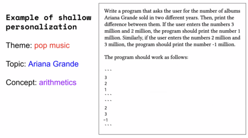
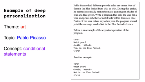
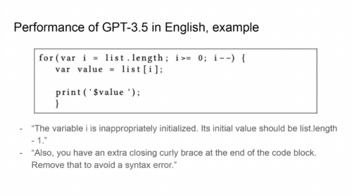
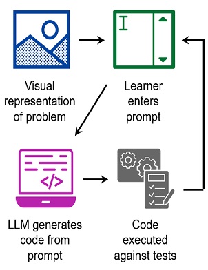
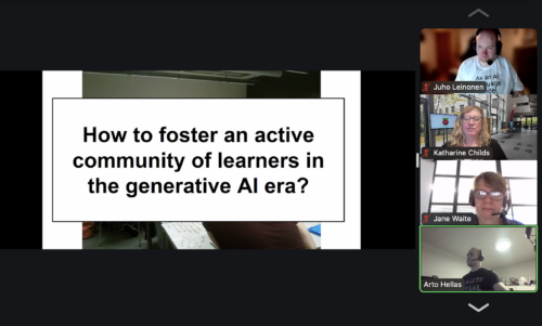


 Francisco Morillo is a Streaming Solutions Architect at AWS. Francisco works with AWS customers, helping them design real-time analytics architectures using AWS services, supporting Amazon Managed Streaming for Apache Kafka (Amazon MSK) and Amazon Managed Service for Apache Flink.
 Anusha Dasarakothapalli is a Principal Software Engineer for Amazon Managed Streaming for Apache Kafka (Amazon MSK) at AWS. She started her software engineering career with Amazon in 2015 and worked on products such as S3-Glacier and S3 Glacier Deep Archive, before transitioning to MSK in 2022. Her primary areas of focus lie in streaming technology, distributed systems, and storage.
 Shakhi Hali is a Principal Product Manager for Amazon Managed Streaming for Apache Kafka (Amazon MSK) at AWS. She is passionate about helping customers generate business value from real-time data. Before joining MSK, Shakhi was a PM with Amazon S3. In her free time, Shakhi enjoys traveling, cooking, and spending time with family.
 Digish Reshamwala is a Software Development Manager for Amazon Managed Streaming for Apache Kafka (Amazon MSK) at AWS. He started his career with Amazon in 2022 and worked on product such as AWS Fargate, before transitioning to MSK in 2024. Before joining AWS, Digish worked at NortonLifelLock and Symantec in engineering roles. He holds an MS degree from University of Southern California. His primary areas of focus lie in streaming technology and distributed computing.

 Minu Hong is a Senior Product Manager for Amazon Kinesis Data Streams at AWS. He is passionate about understanding customer challenges around streaming data and developing optimized solutions for them. Outside of work, Minu enjoys traveling, playing tennis, skiing, and cooking.
 Pratik Patel is a Senior Technical Account Manager and streaming analytics specialist. He works with AWS customers and provides ongoing support and technical guidance to help plan and build solutions using best practices and proactively helps in keeping customers’ AWS environments operationally healthy.
 Priyanka Chaudhary is a Senior Solutions Architect and data analytics specialist. She works with AWS customers as their trusted advisor, providing technical guidance and support in building Well-Architected, innovative industry solutions.


