Post Syndicated from original https://xkcd.com/2610/

Post Syndicated from original https://xkcd.com/2610/
Post Syndicated from original https://lwn.net/Articles/892272/
The Ubuntu 22.04 LTS release, codenamed “Jammy Jellyfish”, is now available. It comes in several editions (Desktop, Server, Cloud, and Core) and multiple flavors (Ubuntu Budgie, Kubuntu, Lubuntu, Ubuntu Kylin, Ubuntu MATE,
UbuntuStudio, and Xubuntu). Lots more information can be found in the release notes.
Ubuntu Desktop 22.04 LTS gains significant usability, battery and performance
improvements with GNOME 42. It features GNOME power profiles and streamlined
workspace transitions alongside significant optimisations which can double
the desktop frame rate on Intel and Raspberry Pi graphics drivers.Ubuntu 22.04 LTS is the first LTS release where the entire recent Raspberry
Pi device portfolio is supported, from the new Raspberry Pi Zero 2W to the
Raspberry Pi 4. Ubuntu 22.04 LTS adds Rust for memory-safe systems-level
programming. It also moves to OpenSSL v3, with new cryptographic algorithms
for elevated security.
Post Syndicated from Scott Rigney original https://aws.amazon.com/blogs/big-data/query-10-new-data-sources-with-amazon-athena/
When we first launched Amazon Athena, our mission was to make it simple to query data stored in Amazon Simple Storage Service (Amazon S3). Athena customers found it easy to get started and develop analytics on petabyte-scale data lakes, but told us they needed to join their Amazon S3 data with data stored elsewhere. We added connectors to sources including Amazon DynamoDB and Amazon Redshift to give data analysts, data engineers, and data scientists the ability to run SQL queries on data stored in databases running on-premises or in the cloud alongside data stored in Amazon S3.
Today, thousands of AWS customers from nearly every industry use Athena federated queries to surface insights and make data-driven decisions from siloed enterprise data—using a single AWS service and SQL dialect.
We’re excited to expand your ability to derive insights from more of your data with today’s release of 10 new data source connectors, which include some of the most widely used data stores on the market.
You can now use Athena to query and surface insights from 10 new data sources:
Today’s release greatly expands the number of data sources supported by Athena. For a complete list of supported data sources, see Using Athena Data Source Connectors.
To coincide with this release, we enhanced the Athena console to help you browse available sources and connect to your data in fewer steps. You can now search, sort, and filter the available connectors on the console, and then follow the guided setup wizard to connect to your data.
Just as before, we’ve open-sourced the new connectors to invite contributions from the developer community. For more information, see Writing a Data Source Connector Using the Athena Query Federation SDK.
With the breadth of data storage options available today, it’s common for data-driven organizations to choose a data store that meets the requirements of specific use cases and applications. Although this flexibility is ideal for architects and developers, it can add complexity for analysts, data scientists, and data engineers, which prevents them from accessing the data they need. To get around this, many users resort to workarounds that often involve learning new programming languages and database concepts or building data pipelines to prepare the data before it can be analyzed. Athena helps cut through this complexity with support for over 25 data sources and its simple-to-use, pay-as-you-go, serverless design.
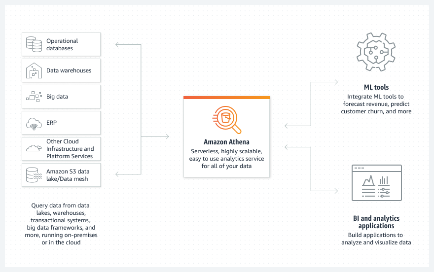
With Athena, you can use your existing SQL knowledge to extract insights from a wide range of data sources without learning a new language, developing scripts to extract (and duplicate) data, or managing infrastructure. Athena allows you to do the following:
To get started with federated queries for Athena, on the Athena console, choose Data Sources in the navigation pane, choose a data source, and follow the guided setup experience to configure your connector. After the connection is established and the source is registered with Athena, you can query the data via the Athena console, API, AWS SDK, and compatible third-party applications. To learn more, see Using Amazon Athena Federated Query and Writing Federated Queries.
You can also share a data source connection with team members, allowing them to use their own AWS account to query the data without setting up a duplicate connector. To learn more, see Enabling Cross-Account Federated Queries.
We encourage you to evaluate Athena and federated queries on your next analytics project. For help getting started, we recommend the following resources:
 Scott Rigney is a Senior Technical Product Manager with Amazon Web Services (AWS) and works with the Amazon Athena team based out of Arlington, Virginia. He is passionate about building analytics products that enable enterprises to make data-driven decisions.
 Jean-Louis Castro-Malaspina is a Senior Product Marketing Manager with Amazon Web Services (AWS) based in Hershey, Pennsylvania. He enjoys highlighting how customers use Analytics and Amazon Athena to unlock innovation. Outside of work, Jean-Louis enjoys spending time with his wife and daughter, running, and following international soccer.
 Suresh Akena is a Principal WW GTM Leader for Amazon Athena. He works with the startups, enterprise and strategic customers to provide leadership on large scale data strategies including migration to AWS platform, big data and analytics and ML initiatives and help them to optimize and improve time to market for data driven applications when using AWS.
Post Syndicated from Benjamin Menuet original https://aws.amazon.com/blogs/big-data/build-your-data-pipeline-in-your-aws-modern-data-platform-using-aws-lake-formation-aws-glue-and-dbt-core/
dbt has established itself as one of the most popular tools in the modern data stack, and is aiming to bring analytics engineering to everyone. The dbt tool makes it easy to develop and implement complex data processing pipelines, with mostly SQL, and it provides developers with a simple interface to create, test, document, evolve, and deploy their workflows. For more information, see docs.getdbt.com.
dbt primarily targets cloud data warehouses such as Amazon Redshift or Snowflake. Now, you can use dbt against AWS data lakes, thanks to the following two services:
In this post, you’ll learn how to deploy a data pipeline in your modern data platform using the dbt-glue adapter built by the AWS Professional Services team in collaboration with dbtlabs.
With this new open-source, battle-tested dbt AWS Glue adapter, developers can now use dbt for their data lakes, paying for just the compute they need, with no need to shuffle data around. They still have access to everything that makes dbt great, including the local developer experience, documentation, tests, incremental data processing, Git integration, CI/CD, and more.
The following diagram shows the architecture of the solution.
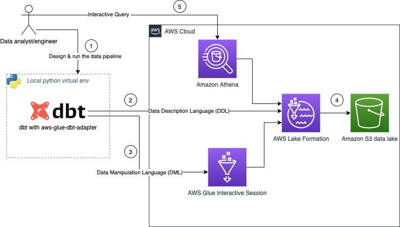
The steps in this workflow are as follows:
dbt-glue adapter uses Lake Formation to perform all structure manipulation, like creation of database, tables. or views.dbt-glue adapter uses AWS Glue interactive sessions as the backend for processing your data.For this post, you run a data pipeline that creates indicators based on NYC taxi data by following these steps:
us-east-1.For our use case, we use the data from the New York City Taxi Records dataset. This dataset is available in the Registry of Open Data on AWS (RODA), which is a repository containing public datasets from AWS resources.
The CloudFormation template creates the nyctaxi database in your AWS Glue Data Catalog and a table (records) that points to the public dataset. You don’t need to host the data in your account.
The CloudFormation template used by this project configures the AWS Identity and Access Management (IAM) role GlueInteractiveSessionRole with all the mandatory permissions.
For more details on permissions for AWS Glue interactive sessions, refer to Securing AWS Glue interactive sessions with IAM.
The CloudFormation stack deploys all the required infrastructure:
dbt-glue adapter.To create these resources, choose Launch Stack and follow the instructions:
![]()
To start working with the shell, complete the following steps:
cloudshell in the Find Services box and then choose the CloudShell option.
dbt and the dbt-glue adapter are compatible with Python versions 3.7, 3.8, and 3.9, check the version of Python:
aws-glue-session package:
The dbt CLI is a command-line interface for running dbt projects. It’s is free to use and available as an open source project. Install dbt and the dbt CLI with the following code:
For more information, refer to How to install dbt, What is dbt?, and Viewpoint.
Install the dbt adapter with the following code:
The dbt AWS Glue interactive session demo project contains an example of a data pipeline that produces metrics based on NYC taxi dataset. Clone the project with the following code:
This project comes with the following configuration example:
The following table summarizes the parameter options for the adaptor.
| Option | Description | Mandatory |
| project_name | The dbt project name. This must be the same as the one configured in the dbt project. | yes |
| type | The driver to use. | yes |
| query-comment | A string to inject as a comment in each query that dbt runs. | no |
| role_arn | The ARN of the interactive session role created as part of the CloudFormation template. | yes |
| region | The AWS Region were you run the data pipeline. | yes |
| workers | The number of workers of a defined workerType that are allocated when a job runs. | yes |
| worker_type | The type of predefined worker that is allocated when a job runs. Accepts a value of Standard, G.1X, or G.2X. | yes |
| schema | The schema used to organize data stored in Amazon S3. | yes |
| database | The database in Lake Formation. The database stores metadata tables in the Data Catalog. | yes |
| session_provisioning_timeout_in_seconds | The timeout in seconds for AWS Glue interactive session provisioning. | yes |
| location | The Amazon S3 location of your target data. | yes |
| idle_timeout | The AWS Glue session idle timeout in minutes. (The session stops after being idle for the specified amount of time.) | no |
| glue_version | The version of AWS Glue for this session to use. Currently, the only valid options are 2.0 and 3.0. The default value is 2.0. | no |
| security_configuration | The security configuration to use with this session. | no |
| connections | A comma-separated list of connections to use in the session. | no |
The objective of this sample project is to create the following four tables, which contain metrics based on the NYC taxi dataset:
This section demonstrates how to query the target table using Athena. To query the data, complete the following steps:
athena-dbt-glue-aws-blog.The following screenshot shows the results of this query.

To clean up your environment, complete the following steps in CloudShell:
This post demonstrates how AWS managed services are key enablers and accelerators to build a modern data platform at scale or take advantage of an existing one.
With the introduction of dbt and aws-glue-dbt-adapter, data teams can access data stored in your modern data platform using SQL statements to extract value from data.
To report a bug or request a feature, please open an issue on GitHub. If you have any questions or suggestions, leave your feedback in the comment section. If you need further assistance to optimize your modern data platform, contact your AWS account team or a trusted AWS Partner.
 Benjamin Menuet is a Data Architect with AWS Professional Services. He helps customers develop big data and analytics solutions to accelerate their business outcomes. Outside of work, Benjamin is a trail runner and has finished some mythic races like the UTMB.
 Armando Segnini is a Data Architect with AWS Professional Services. He spends his time building scalable big data and analytics solutions for AWS Enterprise and Strategic customers. Armando also loves to travel with his family all around the world and take pictures of the places he visits.
 Moshir Mikael is a Senior Practice Manager with AWS Professional Services. He led development of large enterprise data platforms in EMEA and currently leading the Professional Services teams in EMEA for analytics.
 Anouar Zaaber is a Senior Engagement Manager in AWS Professional Services. He leads internal AWS teams, external partners, and customer teams to deliver AWS cloud services that enable customers to realize their business outcomes.
Post Syndicated from Antje Barth original https://aws.amazon.com/blogs/aws/amazon-sagemaker-serverless-inference-machine-learning-inference-without-worrying-about-servers/
In December 2021, we introduced Amazon SageMaker Serverless Inference (in preview) as a new option in Amazon SageMaker to deploy machine learning (ML) models for inference without having to configure or manage the underlying infrastructure. Today, I’m happy to announce that Amazon SageMaker Serverless Inference is now generally available (GA).
Different ML inference use cases pose different requirements on your model hosting infrastructure. If you work on use cases such as ad serving, fraud detection, or personalized product recommendations, you are most likely looking for API-based, online inference with response times as low as a few milliseconds. If you work with large ML models, such as in computer vision (CV) applications, you might require infrastructure that is optimized to run inference on larger payload sizes in minutes. If you want to run predictions on an entire dataset, or larger batches of data, you might want to run an on-demand, one-time batch inference job instead of hosting a model-serving endpoint. And what if you have an application with intermittent traffic patterns, such as a chatbot service or an application to process forms or analyze data from documents? In this case, you might want an online inference option that is able to automatically provision and scale compute capacity based on the volume of inference requests. And during idle time, it should be able to turn off compute capacity completely so that you are not charged.
Amazon SageMaker, our fully managed ML service, offers different model inference options to support all of those use cases:
Amazon SageMaker Serverless Inference in More Detail
In a lot of conversations with ML practitioners, I’ve picked up the ask for a fully managed ML inference option that lets you focus on developing the inference code while managing all things infrastructure for you. SageMaker Serverless Inference now delivers this ease of deployment.
Based on the volume of inference requests your model receives, SageMaker Serverless Inference automatically provisions, scales, and turns off compute capacity. As a result, you pay for only the compute time to run your inference code and the amount of data processed, not for idle time.
You can use SageMaker’s built-in algorithms and ML framework-serving containers to deploy your model to a serverless inference endpoint or choose to bring your own container. If traffic becomes predictable and stable, you can easily update from a serverless inference endpoint to a SageMaker real-time endpoint without the need to make changes to your container image. Using Serverless Inference, you also benefit from SageMaker’s features, including built-in metrics such as invocation count, faults, latency, host metrics, and errors in Amazon CloudWatch.
Since its preview launch, SageMaker Serverless Inference has added support for the SageMaker Python SDK and model registry. SageMaker Python SDK is an open-source library for building and deploying ML models on SageMaker. SageMaker model registry lets you catalog, version, and deploy models to production.
New for the GA launch, SageMaker Serverless Inference has increased the maximum concurrent invocations per endpoint limit to 200 (from 50 during preview), allowing you to use Amazon SageMaker Serverless Inference for high-traffic workloads. Amazon SageMaker Serverless Inference is now available in all the AWS Regions where Amazon SageMaker is available, except for the AWS GovCloud (US) and AWS China Regions.
Several customers have already started enjoying the benefits of SageMaker Serverless Inference:
“Bazaarvoice leverages machine learning to moderate user-generated content to enable a seamless shopping experience for our clients in a timely and trustworthy manner. Operating at a global scale over a diverse client base, however, requires a large variety of models, many of which are either infrequently used or need to scale quickly due to significant bursts in content. Amazon SageMaker Serverless Inference provides the best of both worlds: it scales quickly and seamlessly during bursts in content and reduces costs for infrequently used models.” — Lou Kratz, PhD, Principal Research Engineer, Bazaarvoice
“Transformers have changed machine learning, and Hugging Face has been driving their adoption across companies, starting with natural language processing and now with audio and computer vision. The new frontier for machine learning teams across the world is to deploy large and powerful models in a cost-effective manner. We tested Amazon SageMaker Serverless Inference and were able to significantly reduce costs for intermittent traffic workloads while abstracting the infrastructure. We’ve enabled Hugging Face models to work out of the box with SageMaker Serverless Inference, helping customers reduce their machine learning costs even further.” — Jeff Boudier, Director of Product, Hugging Face
Now, let’s see how you can get started on SageMaker Serverless Inference.
For this demo, I’ve built a text classifier to turn e-commerce customer reviews, such as “I love this product!” into positive (1), neutral (0), and negative (-1) sentiments. I’ve used the Women’s E-Commerce Clothing Reviews dataset to fine-tune a RoBERTa model from the Hugging Face Transformers library and model hub. I will now show you how to deploy the trained model to an Amazon SageMaker Serverless Inference Endpoint.
Deploy Model to an Amazon SageMaker Serverless Inference Endpoint
You can create, update, describe, and delete a serverless inference endpoint using the SageMaker console, the AWS SDKs, the SageMaker Python SDK, the AWS CLI, or AWS CloudFormation. In this first example, I will use the SageMaker Python SDK as it simplifies the model deployment workflow through its abstractions. You can also use the SageMaker Python SDK to invoke the endpoint by passing the payload in line with the request. I will show you this in a bit.
First, let’s create the endpoint configuration with the desired serverless configuration. You can specify the memory size and maximum number of concurrent invocations. SageMaker Serverless Inference auto-assigns compute resources proportional to the memory you select. If you choose a larger memory size, your container has access to more vCPUs. As a general rule of thumb, the memory size should be at least as large as your model size. The memory sizes you can choose are 1024 MB, 2048 MB, 3072 MB, 4096 MB, 5120 MB, and 6144 MB. For my RoBERTa model, let’s configure a memory size of 5120 MB and a maximum of five concurrent invocations.
import sagemaker
from sagemaker.serverless import ServerlessInferenceConfig

serverless_config = ServerlessInferenceConfig(
	memory_size_in_mb=5120,
	max_concurrency=5
)
Now let’s deploy the model. You can use the estimator.deploy() method to deploy the model directly from the SageMaker training estimator, together with the serverless inference endpoint configuration. I also provide my custom inference code in this example.
endpoint_name="roberta-womens-clothing-serverless-1"

estimator.deploy(
	endpoint_name = endpoint_name,
	entry_point="inference.py",
	serverless_inference_config=serverless_config
)
SageMaker Serverless Inference also supports model registry when you use the AWS SDK for Python (Boto3). I will show you how to deploy the model from the model registry later in this post.
Let’s check the serverless inference endpoint settings and deployment status. Go to the SageMaker console and browse to the deployed inference endpoint:

From the SageMaker console, you can also create, update, or delete serverless inference endpoints if needed. In Amazon SageMaker Studio, select the endpoint tab and your serverless inference endpoint to review the endpoint configuration details.

Once the endpoint status shows InService, you can start sending inference requests.
Now, let’s run a few sample predictions. My fine-tuned RoBERTa model expects the inference requests in JSON Lines format with the review text to classify as the input feature. A JSON Lines text file comprises several lines where each individual line is a valid JSON object, delimited by a newline character. This is an ideal format for storing data that is processed one record at a time, such as in model inference. You can learn more about JSON Lines and other common data formats for inference in the Amazon SageMaker Developer Guide. Note that the following code might look different depending on your model’s accepted inference request format.
from sagemaker.predictor import Predictor
from sagemaker.serializers import JSONLinesSerializer
from sagemaker.deserializers import JSONLinesDeserializer

sess = sagemaker.Session(sagemaker_client=sm)

inputs = [
    {"features": ["I love this product!"]},
    {"features": ["OK, but not great."]},
    {"features": ["This is not the right product."]},
]

predictor = Predictor(
    endpoint_name=endpoint_name,
    serializer=JSONLinesSerializer(),
    deserializer=JSONLinesDeserializer(),
    sagemaker_session=sess
)

predicted_classes = predictor.predict(inputs)

for predicted_class in predicted_classes:
    print("Predicted class {} with probability {}".format(predicted_class['predicted_label'], predicted_class['probability']))
The result will look similar to this, classifying the sample reviews into the corresponding sentiment classes.
Predicted class 1 with probability 0.9495596289634705
Predicted class 0 with probability 0.5395089387893677
Predicted class -1 with probability 0.7887083292007446
You can also deploy your model from the model registry to a SageMaker Serverless Inference endpoint. This is currently only supported through the AWS SDK for Python (Boto3). Let me walk you through another quick demo.
Deploy Model from the SageMaker Model Registry
To deploy the model from the model registry using Boto3, let’s first create a model object from the model version by calling the create_model() method. Then, I pass the Amazon Resource Name (ARN) of the model version as part of the containers for the model object.
import boto3
import sagemaker

sm = boto3.client(service_name='sagemaker')
role = sagemaker.get_execution_role()
model_name="roberta-womens-clothing-serverless"

container_list =
	[{'ModelPackageName': <MODEL_PACKAGE_ARN>}]

create_model_response = sm.create_model(
    ModelName = model_name,
    ExecutionRoleArn = role,
    Containers = container_list
)
Next, I create the serverless inference endpoint. Remember that you can create, update, describe, and delete a serverless inference endpoint using the SageMaker console, the AWS SDKs, the SageMaker Python SDK, the AWS CLI, or AWS CloudFormation. For consistency, I keep using Boto3 in this second example.
Similar to the first example, I start by creating the endpoint configuration with the desired serverless configuration. I specify the memory size of 5120 MB and a maximum number of five concurrent invocations for my endpoint.
endpoint_config_name="roberta-womens-clothing-serverless-ep-config"

create_endpoint_config_response = sm.create_endpoint_config(
    EndpointConfigName = endpoint_config_name,
    ProductionVariants=[{
        'ServerlessConfig':{
            'MemorySizeInMB' : 5120,
            'MaxConcurrency' : 5
        },
        'ModelName':model_name,
        'VariantName':'AllTraffic'}])
Next, I create the SageMaker Serverless Inference endpoint by calling the create_endpoint() method.
endpoint_name="roberta-womens-clothing-serverless-2"

create_endpoint_response = sm.create_endpoint(
    EndpointName=endpoint_name,
    EndpointConfigName=endpoint_config_name)
Once the endpoint status shows InService, you can start sending inference requests. Again, for consistency, I choose to run the sample prediction using Boto3 and the SageMaker runtime client invoke_endpoint() method.
sm_runtime = boto3.client("sagemaker-runtime")
response = sm_runtime.invoke_endpoint(
    EndpointName=endpoint_name,
    ContentType="application/jsonlines",
    Accept="application/jsonlines",
    Body=bytes('{"features": ["I love this product!"]}', 'utf-8')
)

print(response['Body'].read().decode('utf-8'))
{"probability": 0.966135561466217, "predicted_label": 1}
How to Optimize Your Model for SageMaker Serverless Inference
SageMaker Serverless Inference automatically scales the underlying compute resources to process requests. If the endpoint does not receive traffic for a while, it scales down the compute resources. If the endpoint suddenly receives new requests, you might notice that it takes some time for the endpoint to scale up the compute resources to process the requests.
This cold-start time greatly depends on your model size and the start-up time of your container. To optimize cold-start times, you can try to minimize the size of your model, for example, by applying techniques such as knowledge distillation, quantization, or model pruning.
Knowledge distillation uses a larger model (the teacher model) to train smaller models (student models) to solve the same task. Quantization reduces the precision of the numbers representing your model parameters from 32-bit floating-point numbers down to either 16-bit floating-point or 8-bit integers. Model pruning removes redundant model parameters that contribute little to the training process.
Availability and Pricing
Amazon SageMaker Serverless Inference is now available in all the AWS Regions where Amazon SageMaker is available except for the AWS GovCloud (US) and AWS China Regions.
With SageMaker Serverless Inference, you only pay for the compute capacity used to process inference requests, billed by the millisecond, and the amount of data processed. The compute capacity charge also depends on the memory configuration you choose. For detailed pricing information, visit the SageMaker pricing page.
Get Started Today with Amazon SageMaker Serverless Inference
To learn more about Amazon SageMaker Serverless Inference, visit the Amazon SageMaker machine learning inference webpage. Here are SageMaker Serverless Inference example notebooks that will help you get started right away. Give them a try from the SageMaker console, and let us know what you think.
– Antje
Post Syndicated from Kareem Syed-Mohammed original https://aws.amazon.com/blogs/big-data/amazon-quicksight-1-click-public-embedding-available-in-preview/
Amazon QuickSight is a fully managed, cloud-native business intelligence (BI) service that makes it easy to connect to your data, create interactive dashboards, and share these with tens of thousands of users, either directly within a QuickSight application, or embedded in web apps and portals.
QuickSight Enterprise Edition now supports 1-click public embedding, a feature that allows you to embed your dashboards into public applications, wikis, and portals without any coding or development needed. Anyone on the internet can start accessing these embedded dashboards with up-to-date information instantly, without any server deployments or infrastructure licensing needed! 1-click public embedding allows you to empower your end-users with access to insights.
In this post, we walk you through the steps to use this feature, demonstrate the end-user experience, and share sample use cases.
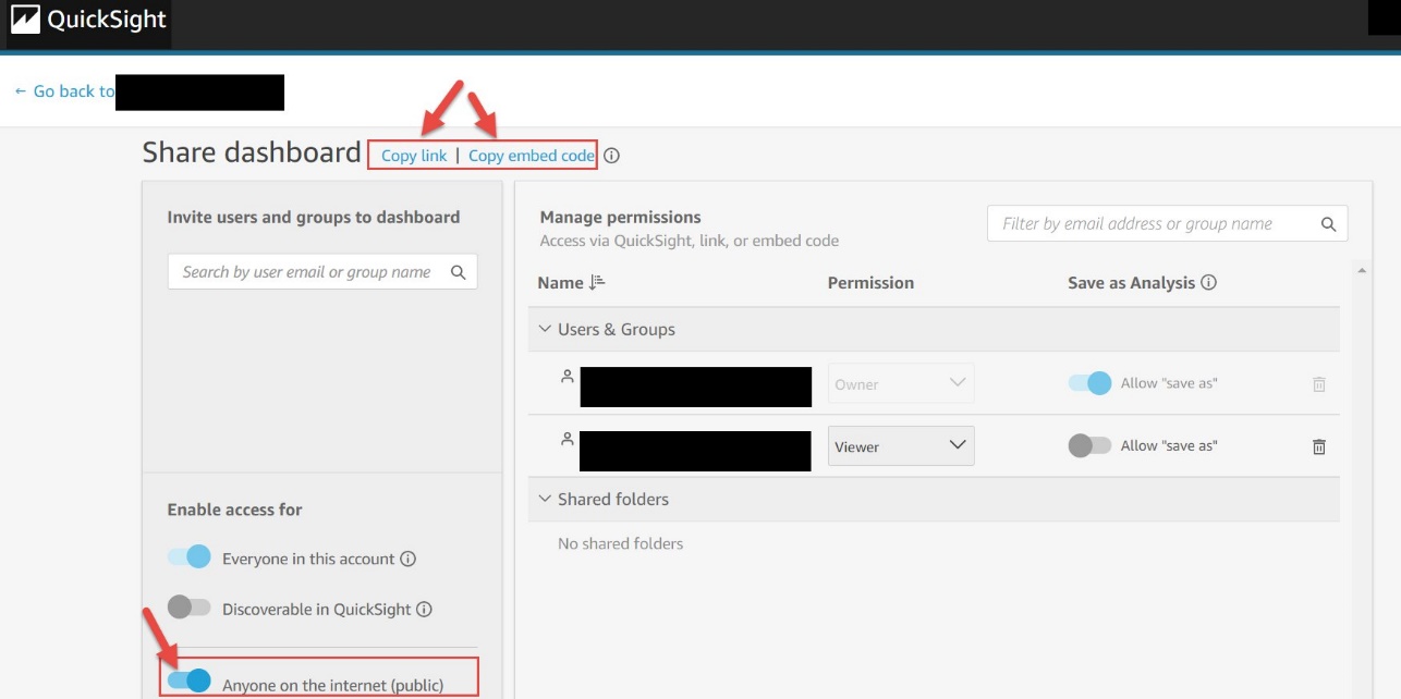
1-click public embedding requires an administrator of the QuickSight account to enable this feature and use session-based pricing. After you complete the prerequisites (see the following section), the 1-click embedding process involves three simple steps:
After you enable this policy, you can activate the account-level settings.


Enabling this setting doesn’t automatically enable all the dashboards to be accessed by anyone on the internet. It gives the ability for authors of the dashboards to individually enable the dashboard to be accessed by anyone on the internet via the share link or when embedded.
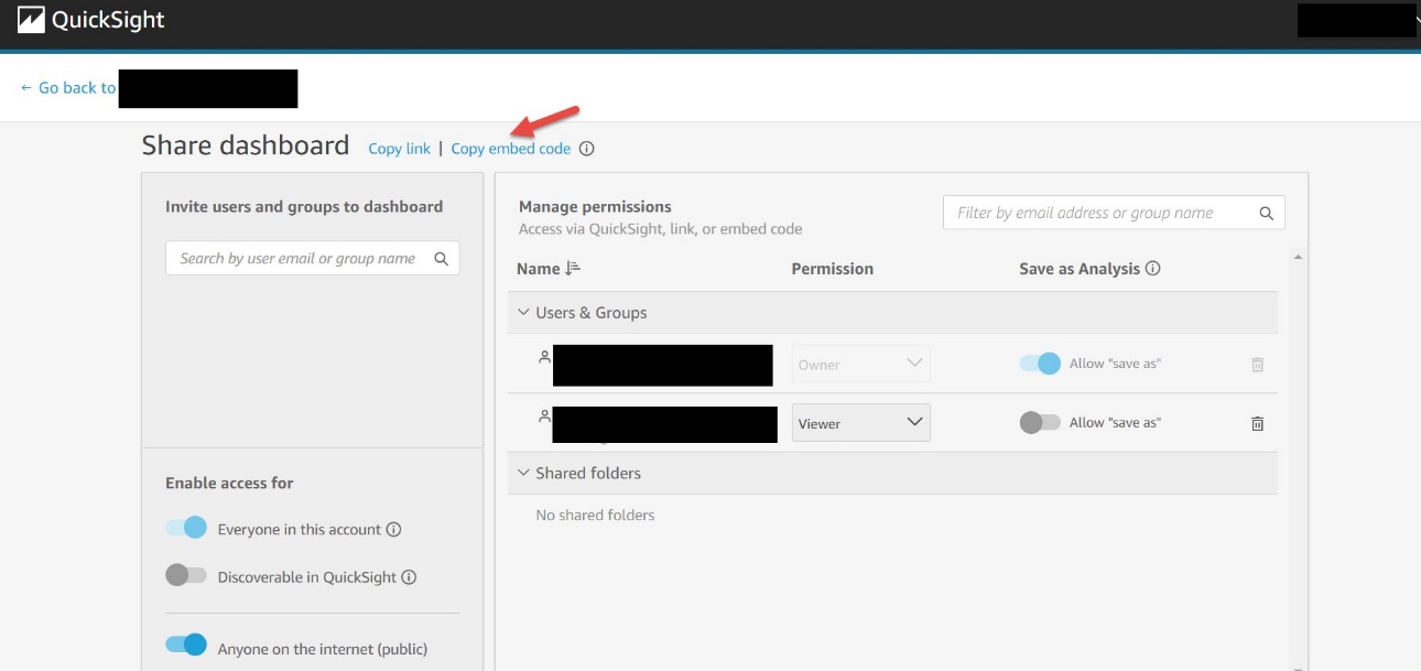
After you create a QuickSight dashboard, to enable public access, complete the following steps:
Only owners and co-owners of the dashboard can perform this action.
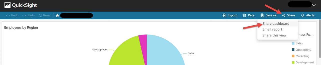

This setting allows you to share this dashboard with anyone on the internet via the share link or when embedded.
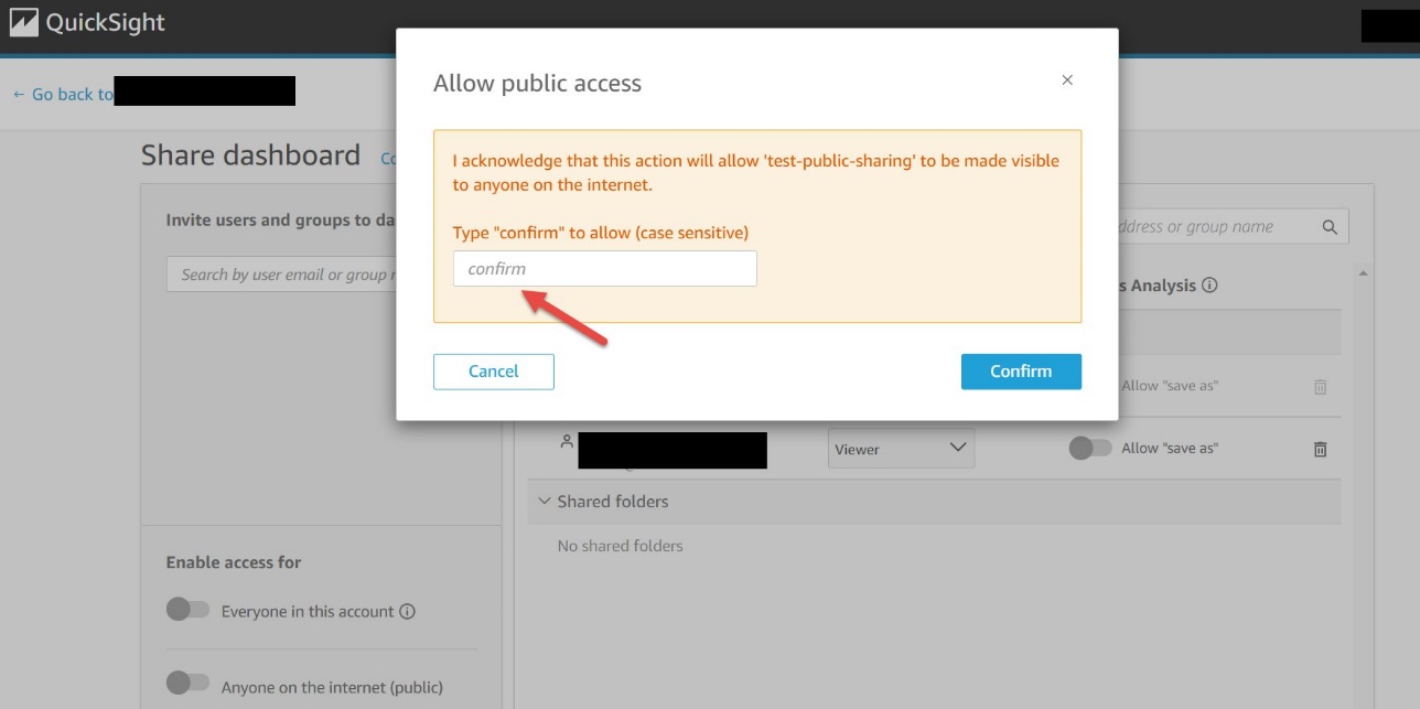
You now have the option to copy the link or the embed code to share the dashboard. Note that when this setting is enabled, the dashboard can only be accessed using the link or when embedded using the embed code.
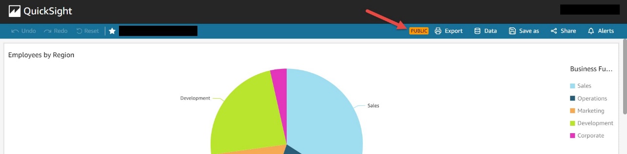
After you enable the dashboard for public access, you can see badges on the dashboard as follows.
The dashboard toolbar has a PUBLIC badge.
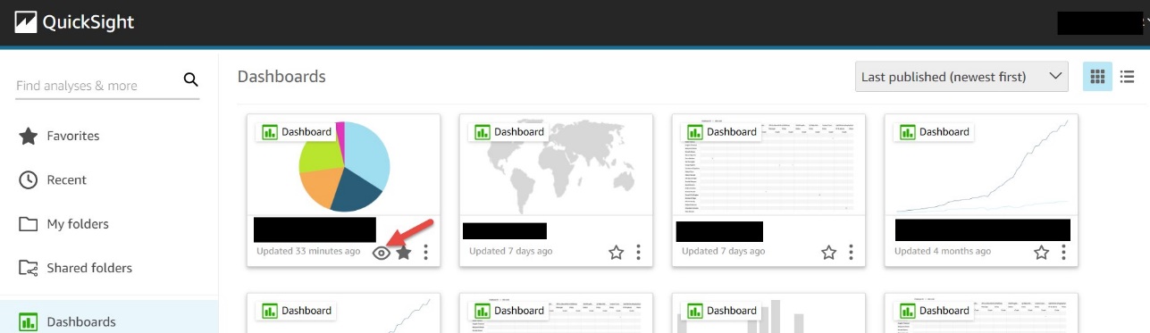
The dashboards grid view has an eye icon for each dashboard.
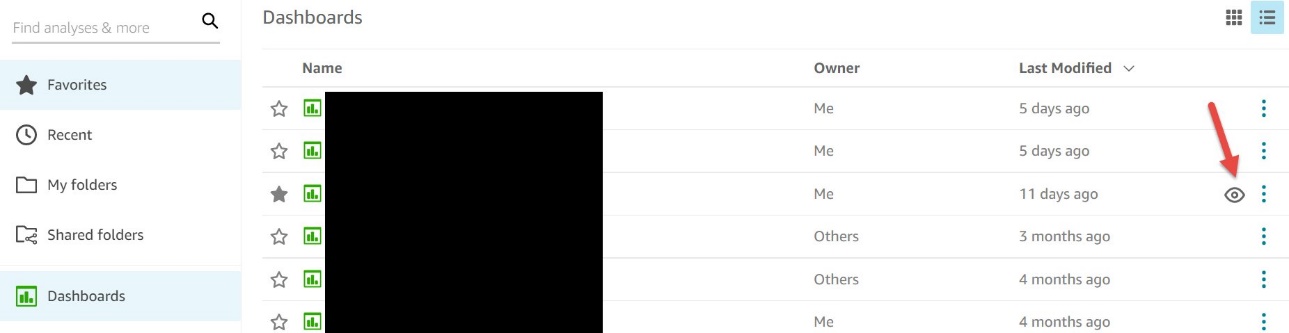
The dashboards list view has an eye icon for each dashboard.
You can disable the public access of your dashboards in two ways:
The domain where the dashboard is to be embedded must be allow listed in QuickSight. For instructions, see Adding domains for embedded users.
After you set your desired access to the dashboard, you can choose Copy embed code, which copies the embed code for that dashboard. This code embeds the dashboard when added to an internal application.
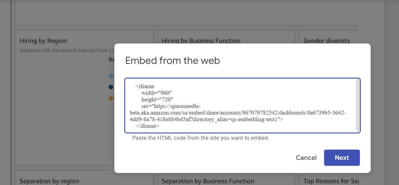
The copied embed code is similar to the following code:
To embed the dashboard in an HTML page, open the HTML of the page where you want to embed the dashboard and enter the copied embed code into the HTML code.
If your public-facing applications are built on Google Sites, to embed your dashboard, open the page on Google Sites, then choose Insert and Embed. A pop-up window appears with a prompt to enter a URL or embed code. Choose Embed code and enter the copied embed code in the text box.
Make sure to allow list the following domains in QuickSight when embedding in Google Sites: https://googleusercontent.com (enable subdomains), https://www.gstatic.com, and https://sites.google.com.
After you embed the dashboard in your application, anyone who can access your application can now access the embedded dashboard.

1-click public embedding enables you to embed your dashboards into public applications, wikis, and portals without any coding or development needed. In this section, we present two sample use cases.
For our first use case, a fictitious school district uses 1-click public embedding to report on the teachers’ enrollment in the district. They built a dashboard and used this feature to embed it on their public-facing site.

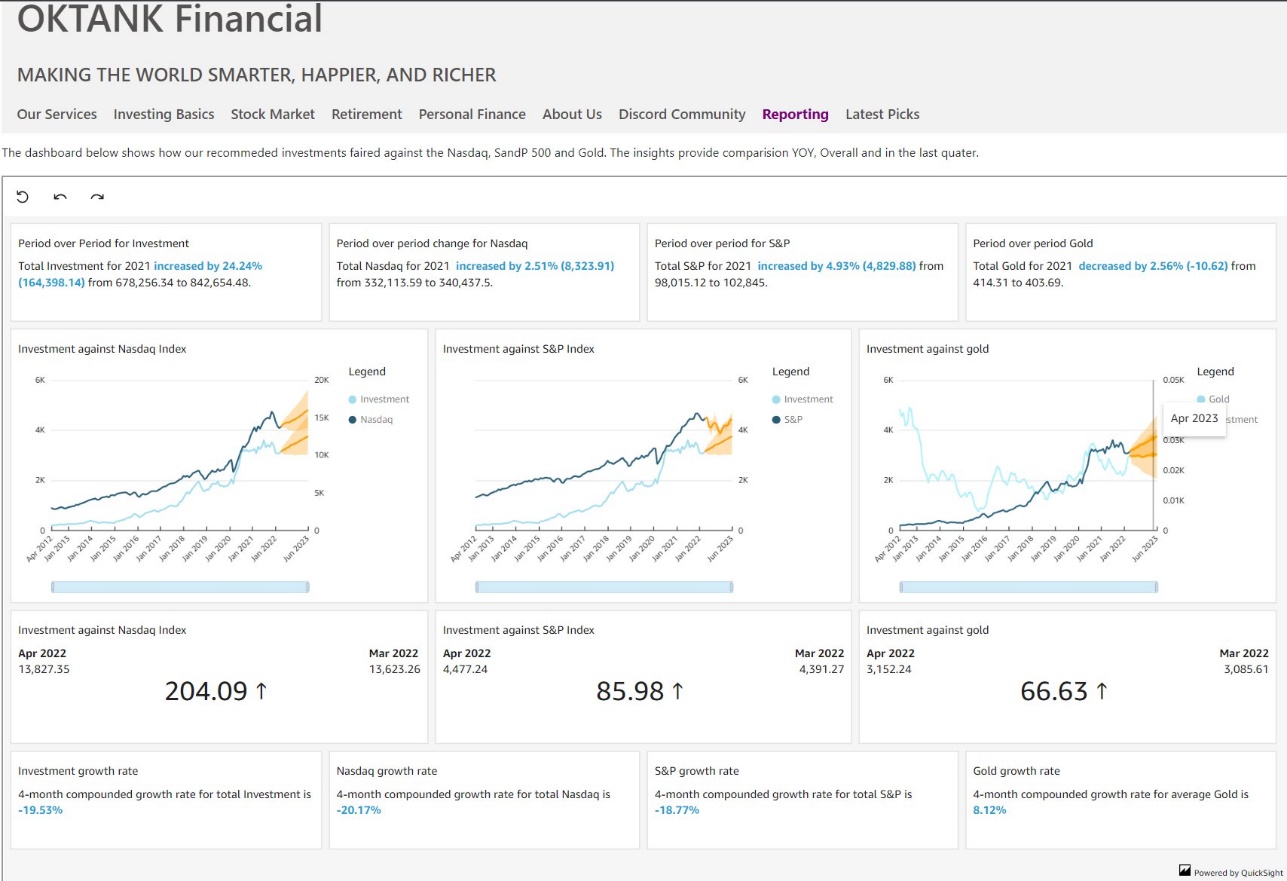
For our second use case, a fictitious fintech that provides investment solutions is using 1-click public embedding to show how their investment compares against other well-known indexes and commodities. They used this feature to add this comparison dashboard on their public-facing marketing pages.
To try out this feature, see Embed Amazon QuickSight dashboard in seconds. In this demo, you can change the dashboard between a logistics or sales dashboard by choosing Change Dashboard and entering the embed code for the dashboard you want to render on the site.
With 1-click public embedding, you can now embed rich and interactive QuickSight dashboards quickly and easily. Enable your end-users to dive deeper into their data through embedded dashboard with the click of a button—and with no infrastructure setup or management, scale to millions of users. 1-click public embedding is now in preview; to access this feature, please contact [email protected].
QuickSight also supports embedding in SaaS apps without any user management needed. For more information, refer to Embed multi-tenant dashboards in SaaS apps using Amazon QuickSight without provisioning or managing users.
To stay up to date on QuickSight embedded analytics, check out what’s new with the QuickSight User Guide.
 Kareem Syed-Mohammed is a Product Manager at Amazon QuickSight. He focuses on embedded analytics, APIs, and developer experience. Prior to QuickSight he has been with AWS Marketplace and Amazon retail as a PM. Kareem started his career as a developer and then PM for call center technologies, Local Expert and Ads for Expedia. He worked as a consultant with McKinsey and Company for a short while.
 Srikanth Baheti is a Specialized World Wide Sr. Solution Architect for Amazon QuickSight. He started his career as a consultant and worked for multiple private and government organizations. Later he worked for PerkinElmer Health and Sciences & eResearch Technology Inc, where he was responsible for designing and developing high traffic web applications, highly scalable and maintainable data pipelines for reporting platforms using AWS services and Serverless computing.-
Post Syndicated from Noritaka Sekiyama original https://aws.amazon.com/blogs/big-data/introducing-aws-glue-auto-scaling-automatically-resize-serverless-computing-resources-for-lower-cost-with-optimized-apache-spark/
Data created in the cloud is growing fast in recent days, so scalability is a key factor in distributed data processing. Many customers benefit from the scalability of the AWS Glue serverless Spark runtime. Today, we’re pleased to announce the release of AWS Glue Auto Scaling, which helps you scale your AWS Glue Spark jobs automatically based on the requirements calculated dynamically during the job run, and accelerate job runs at lower cost without detailed capacity planning.
Before AWS Glue Auto Scaling, you had to predict workload patterns in advance. For example, in cases when you don’t have expertise in Apache Spark, when it’s the first time you’re processing the target data, or when the volume or variety of the data is significantly changing, it’s not so easy to predict the workload and plan the capacity for your AWS Glue jobs. Under-provisioning is error-prone and can lead to either missed SLA or unpredictable performance. On the other hand, over-provisioning can cause underutilization of resources and cost overruns. Therefore, it was a common best practice to experiment with your data, monitor the metrics, and adjust the number of AWS Glue workers before you deployed your Spark applications to production.
With AWS Glue Auto Scaling, you no longer need to plan AWS Glue Spark cluster capacity in advance. You can just set the maximum number of workers and run your jobs. AWS Glue monitors the Spark application execution, and allocates more worker nodes to the cluster in near-real time after Spark requests more executors based on your workload requirements. When there are idle executors that don’t have intermediate shuffle data, AWS Glue Auto Scaling removes the executors to save the cost.
AWS Glue Auto Scaling is available with the optimized Spark runtime on AWS Glue version 3.0, and you can start using it today. This post describes possible use cases and how it works.
Traditionally, AWS Glue launches a serverless Spark cluster of a fixed size. The computing resources are held for the whole job run until it is completed. With the new AWS Glue Auto Scaling feature, after you enable it for your AWS Glue Spark jobs, AWS Glue dynamically allocates compute resource considering the given maximum number of workers. It also supports dynamic scale-out and scale-in of the AWS Glue Spark cluster size over the course of job. As more executors are requested by Spark, more AWS Glue workers are added to the cluster. When the executor has been idle without active computation tasks for a period of time and associated shuffle dependencies, the executor and corresponding worker are removed.
AWS Glue Auto Scaling makes it easy to run your data processing in the following typical use cases:
AWS Glue Auto Scaling is available with the optimized Spark runtime on Glue version 3.0. To enable Auto Scaling on the AWS Glue Studio console, complete the following steps:
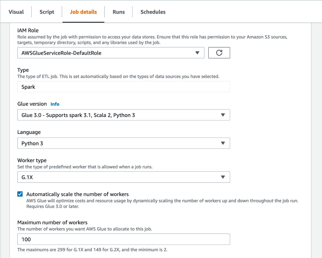
To enable Auto Scaling in the AWS Glue API or AWS Command Line Interface (AWS CLI), set the following job parameters:
--enable-auto-scalingtrueIn this section, we discuss three ways to monitor AWS Glue Auto Scaling: via Amazon CloudWatch metrics or Spark UI.
After you enable AWS Glue Auto Scaling, Spark dynamic allocation is enabled and the executor metrics are visible in CloudWatch. You can review the following metrics to understand the demand and optimized usage of executors in their Spark applications enabled with Auto Scaling:
glue.driver.ExecutorAllocationManager.executors.numberAllExecutorsglue.driver.ExecutorAllocationManager.executors.numberMaxNeededExecutors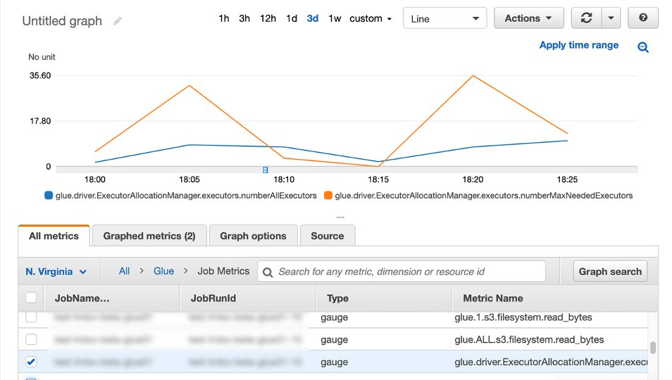
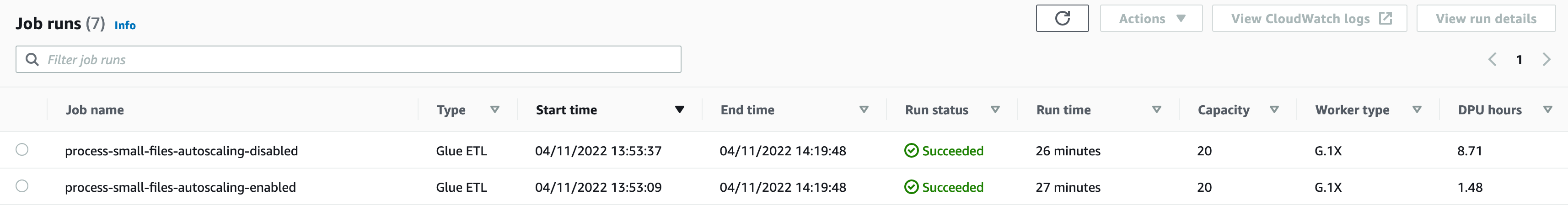
In the Monitoring page in AWS Glue Studio, you can monitor the DPU hours you spent for a specific job run. The following screenshot shows two job runs that processed the same dataset; one without Auto Scaling which spent 8.71 DPU hours, and another one with Auto Scaling enabled which spent only 1.48 DPU hours. The DPU hour values per job run are also available with GetJobRun API responses.
With the Spark UI, you can monitor that the AWS Glue Spark cluster dynamically scales out and scales in with AWS Glue Auto Scaling. The event timeline shows when each executor is added and removed gradually over the Spark application run.

In the following sections, we demonstrate AWS Glue Auto Scaling with two use cases: jobs with driver-heavy workloads, and jobs with multiple stages.
A typical workload for AWS Glue Spark jobs is to process many small files to prepare the data for further analysis. For such workloads, AWS Glue has built-in optimizations, including file grouping, a Glue S3 Lister, partition pushdown predicates, partition indexes, and more. For more information, see Optimize memory management in AWS Glue. All those optimizations execute on the Spark driver and speed up the planning phase on Spark driver to compute and distribute the work for parallel processing with Spark executors. However, without AWS Glue Auto Scaling, Spark executors are idle during the planning phase. With Auto Scaling, Glue jobs only allocate executors when the driver work is complete, thereby saving executor cost.
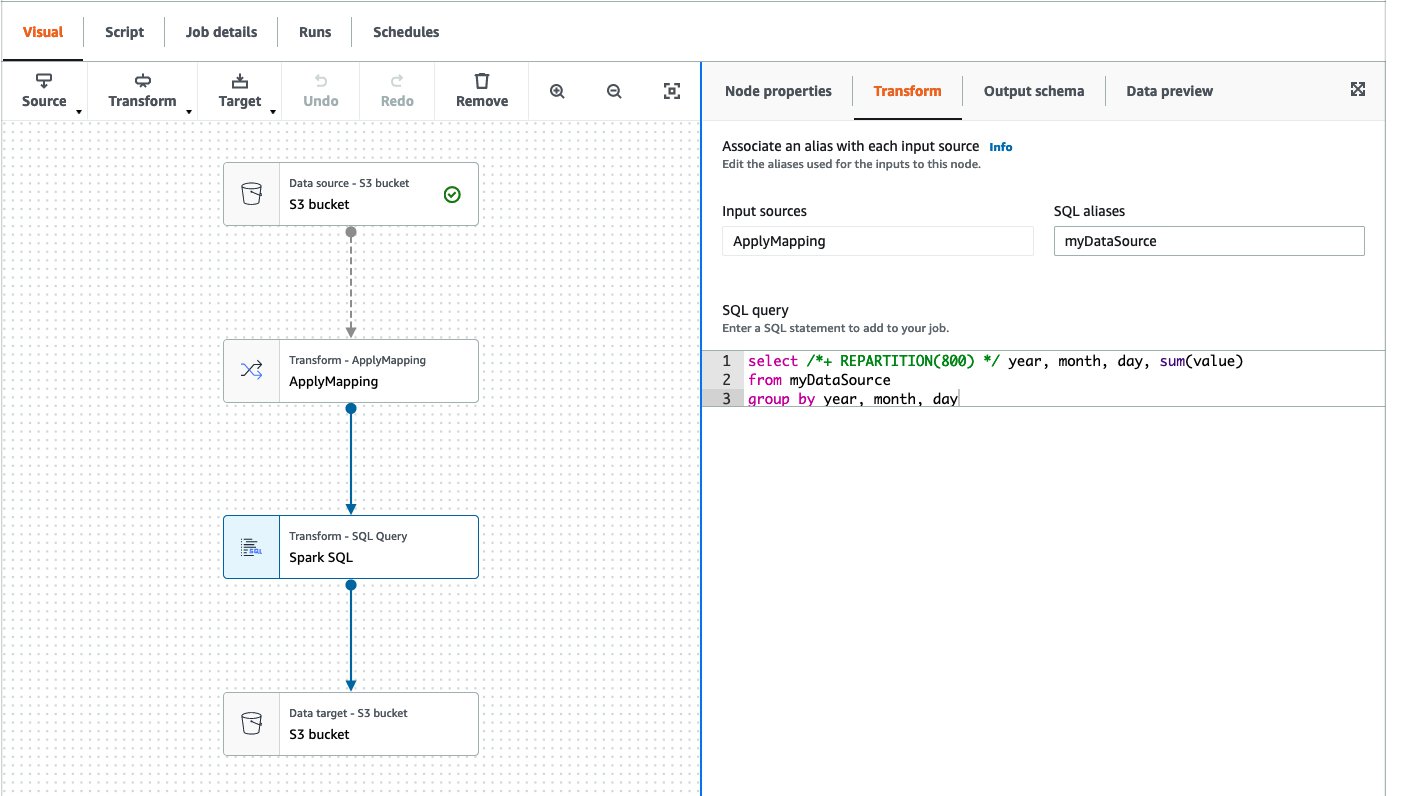
Here’s the example DAG shown in AWS Glue Studio. This AWS Glue job reads from an Amazon Simple Storage Service (Amazon S3) bucket, performs the ApplyMapping transformation, runs a simple SELECT query repartitioning data to have 800 partitions, and writes back to another location in Amazon S3.
The following screenshot shows the executor timeline in Spark UI when the AWS Glue job ran with 20 workers without Auto Scaling. You can confirm that all 20 workers started at the beginning of the job run.

In contrast, the following screenshot shows the executor timeline of the same job with Auto Scaling enabled and the maximum workers set to 20. The driver and one executor started at the beginning, and other executors started only after the driver finished its computation for listing 367,920 partitions on the S3 bucket. These 19 workers were not charged during the long-running driver task.
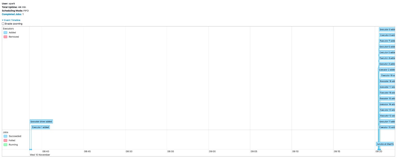
Both jobs completed in 44 minutes. With AWS Glue Auto Scaling, the job completed in the same amount of time with lower cost.
Another typical workload in AWS Glue is to read from the data store or large compressed files, repartition it to have more parallelism for downstream processing, and process further analytic queries. For example, when you want to read from a JDBC data store, you may not want to have many concurrent connections, so you can avoid impacting source database performance. For such workloads, you can have a small number of connections to read data from the JDBC data store, then repartition the data with higher parallelism for further analysis.
Here’s the example DAG shown in AWS Glue Studio. This AWS Glue job reads from the JDBC data source, runs a simple SELECT query adding one more column (mod_id) calculated from the column ID, performs the ApplyMapping node, then writes to an S3 bucket with partitioning by this new column mod_id. Note that the JDBC data source was already registered in the AWS Glue Data Catalog, and the table has two parameters, hashfield=id and hashpartitions=5, to read from JDBC through five concurrent connections.

The following screenshot shows the executor timeline in the Spark UI when the AWS Glue job ran with 20 workers without Auto Scaling. You can confirm that all 20 workers started at the beginning of the job run.

The following screenshot shows the same executor timeline in the Spark UI with Auto Scaling enabled with 20 maximum workers. The driver and two executors started at the beginning, and other executors started later. The first two executors read data from the JDBC source with fewer number of concurrent connections. Later, the job increased parallelism and more executors were started. You can also observe that there were 16 executors, not 20, which further reduced cost.

This post discussed AWS Glue Auto Scaling, which automatically resizes the computing resources of your AWS Glue Spark job capacity and reduce cost. You can start using AWS Glue Auto Scaling for both your existing workloads and future new workloads, and take advantage of it today! For more information about AWS Glue Auto Scaling, see Using Auto Scaling for AWS Glue. Migrate your jobs to Glue version 3.0 and get the benefits of Auto Scaling.
Special thanks to everyone who contributed to the launch: Raghavendhar Thiruvoipadi Vidyasagar, Ping-Yao Chang, Shashank Bhardwaj, Sampath Shreekantha, Vaibhav Porwal, and Akash Gupta.
 Noritaka Sekiyama is a Principal Big Data Architect on the AWS Glue team. He is passionate about architecting fast-growing data platforms, diving deep into distributed big data software like Apache Spark, building reusable software artifacts for data lakes, and sharing the knowledge in AWS Big Data blog posts. In his spare time, he enjoys taking care of killifish, hermit crabs, and grubs with his children.
 Bo Li is a Software Development Engineer on the AWS Glue team. He is devoted to designing and building end-to-end solutions to address customers’ data analytic and processing needs with cloud-based, data-intensive technologies.
 Rajendra Gujja is a Software Development Engineer on the AWS Glue team. He is passionate about distributed computing and everything and anything about data.
 Mohit Saxena is a Senior Software Development Manager on the AWS Glue team. His team works on distributed systems for efficiently managing data lakes on AWS and optimizes Apache Spark for performance and reliability.
Post Syndicated from Marcia Villalba original https://aws.amazon.com/blogs/aws/amazon-aurora-serverless-v2-is-generally-available-instant-scaling-for-demanding-workloads/
Today we are very excited to announce that Amazon Aurora Serverless v2 is generally available for both Aurora PostgreSQL and MySQL. Aurora Serverless is an on-demand, auto-scaling configuration for Amazon Aurora that allows your database to scale capacity up or down based on your application’s needs.
Amazon Aurora is a MySQL- and PostgreSQL-compatible relational database built for the cloud. It is fully managed by Amazon Relational Database Service (RDS), which automates time-consuming administrative tasks, such as hardware provisioning, database setup, patches, and backups.
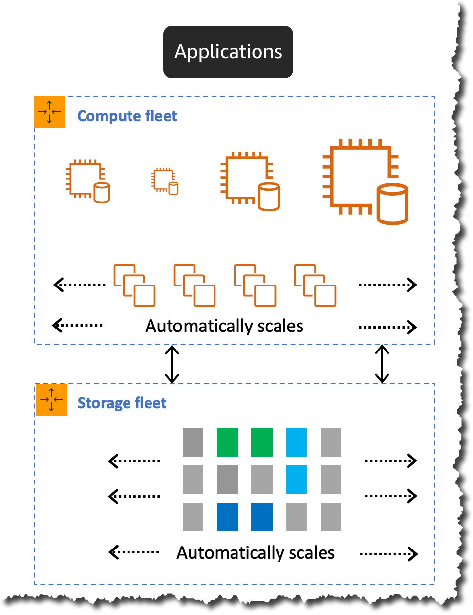
One of the key features of Amazon Aurora is the separation of compute and storage. As a result, they scale independently. Amazon Aurora storage automatically scales as the amount of data in your database increases. For example, you can store lots of data, and if one day you decide to drop most of the data, the storage provisioned adjusts.
However, many customers said that they need the same flexibility in the compute layer of Amazon Aurora since most database workloads don’t need a constant amount of compute. Workloads can be spiky, infrequent, or have predictable spikes over a period of time.
To serve these kinds of workloads, you need to provision for the peak capacity you expect your database will need. However, this approach is expensive as database workloads rarely run at peak capacity. To provision the right amount of compute, you need to continuously monitor the database capacity consumption and scale up resources if consumption is high. However, this requires expertise and often incurs downtime.
To solve this problem, in 2018, we launched the first version of Amazon Aurora Serverless. Since its launch, thousands of customers have used Amazon Aurora Serverless as a cost-effective option for infrequent, intermittent, and unpredictable workloads.
Today, we are making the next version of Amazon Aurora Serverless generally available, which enables customers to run even the most demanding workload on serverless with instant and nondisruptive scaling, fine-grained capacity adjustments, and additional functionality, including read replicas, Multi-AZ deployments, and Amazon Aurora Global Database.
Aurora Serverless v2 is launching with the latest major versions available on Amazon Aurora. Versions supported: Aurora PostgreSQL-compatible edition with PostgreSQL 13 and Aurora MySQL-compatible edition with MySQL 8.0.
Main features of Aurora Serverless v2
Aurora Serverless v2 enables you to scale your database to hundreds of thousands of transactions per second and cost-effectively manage the most demanding workloads. It scales database capacity in fine-grained increments to closely match the needs of your workload without disrupting connections or transactions. In addition, you pay only for the exact capacity you consume, and you can save up to 90 percent compared to provisioning for peak load.
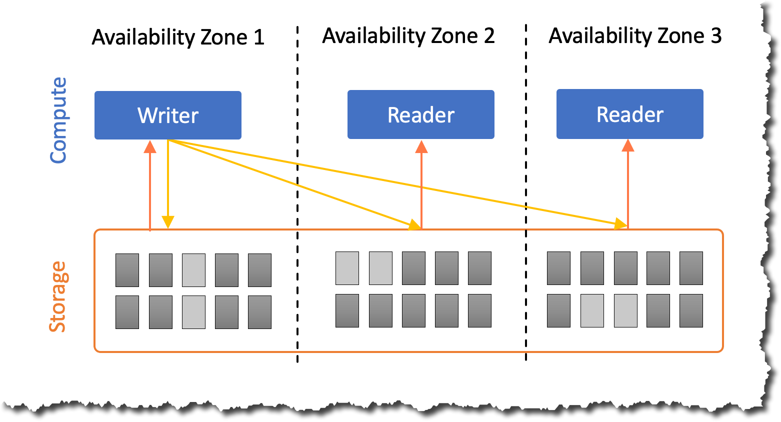
If you have an existing Amazon Aurora cluster, you can create an Aurora Serverless v2 instance within the same cluster. This way, you’ll have a mixed configuration cluster where both provisioned and Aurora Serverless v2 instances can coexist within the same cluster.
It supports the full breadth of Amazon Aurora features. For example, you can create up to 15 Amazon Aurora read replicas deployed across multiple Availability Zones. Any number of these read replicas can be Aurora Serverless v2 instances and can be used as failover targets for high availability or for scaling read operations.
Similarly, with Global Database, you can assign any of the instances to be Aurora Serverless v2 and only pay for minimum capacity when idling. These instances in secondary Regions can also scale independently to support varying workloads across different Regions. Check out the Amazon Aurora user guide for a comprehensive list of features.
How Aurora Serverless v2 scaling works
Aurora Serverless v2 scales instantly and nondisruptively by growing the capacity of the underlying instance in place by adding more CPU and memory resources. This technique allows for the underlying instance to increase and decrease capacity in place without failing over to a new instance for scaling.
For scaling down, Aurora Serverless v2 takes a more conservative approach. It scales down in steps until it reaches the required capacity needed for the workload. Scaling down too quickly can prematurely evict cached pages and decrease the buffer pool, which may affect the performance.
Aurora Serverless capacity is measured in Aurora capacity units (ACUs). Each ACU is a combination of approximately 2 gibibytes (GiB) of memory, corresponding CPU, and networking. With Aurora Serverless v2, your starting capacity can be as small as 0.5 ACU, and the maximum capacity supported is 128 ACU. In addition, it supports fine-grained increments as small as 0.5 ACU which allows your database capacity to closely match the workload needs.
Aurora Serverless v2 scaling in action
To show Aurora Serverless v2 in action, we are going to simulate a flash sale. Imagine that you run an e-commerce site. You run a marketing campaign where customers can purchase items 50 percent off for a limited amount of time. You are expecting a spike in traffic on your site for the duration of the sale.
When you use a traditional database, if you run those marketing campaigns regularly, you need to provision for the peak load you expect. Or, if you run them now and then, you need to reconfigure your database for the expected peak of traffic during the sale. In both cases, you are limited to your assumption of the capacity you need. What happens if you have more sales than you expected? If your database cannot keep up with the demand, it may cause service degradation. Or when your marketing campaign doesn’t produce the sales you expected? You are unnecessarily paying for capacity you don’t need.
For this demo, we use Aurora Serverless v2 as the transactional database. An AWS Lambda function is used to call the database and process orders during the sale event for the e-commerce site. The Lambda function and the database are in the same Amazon Virtual Private Cloud (VPC), and the function connects directly to the database to perform all the operations.
To simulate the traffic of a flash sale, we will use an open-source load testing framework called Artillery. It will allow us to generate varying load by invoking multiple Lambda functions. For example, we can start with a small load and then increase it rapidly to observe how the database capacity adjusts based on the workload. This Artillery load test runs on an Amazon Elastic Compute Cloud (Amazon EC2) instance inside the same VPC.
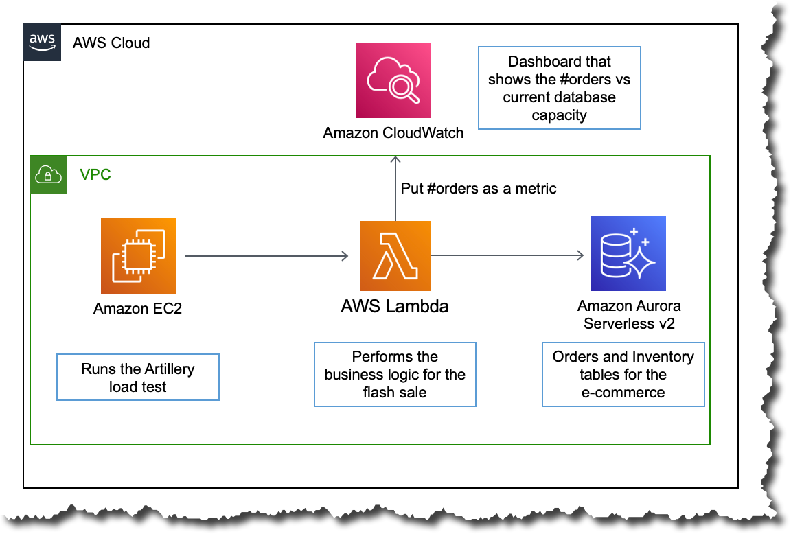
The following Amazon CloudWatch dashboard shows how the database capacity behaves when the order count increases. The dashboard shows the orders placed in blue and the current database capacity in orange.
At the beginning of the sale, the Aurora Serverless v2 database starts with a capacity of 5 ACUs, which was the minimum database capacity configured. For the first few minutes, the orders increase, but the database capacity doesn’t increase right away. The database can handle the load with the starting provisioned capacity.
However, around the time 15:55, the number of orders spikes to 12,000. As a result, the database increases the capacity to 14 ACUs. The database capacity increases in milliseconds, adjusting exactly to the load.
The number of orders placed stays up for some seconds, and then it goes dramatically down by 15:58. However, the database capacity doesn’t adjust exactly to the drop in traffic. Instead, it decreases in steps until it reaches 5 ACUs. The scaling down is done more conservatively to avoid prematurely evicting cached pages and affecting performance. This is done to prevent any unnecessary latency to spiky workloads, and also so the caches and buffer pools are not aggressively purged.

Get started with Aurora Serverless v2 with an existing Amazon Aurora cluster
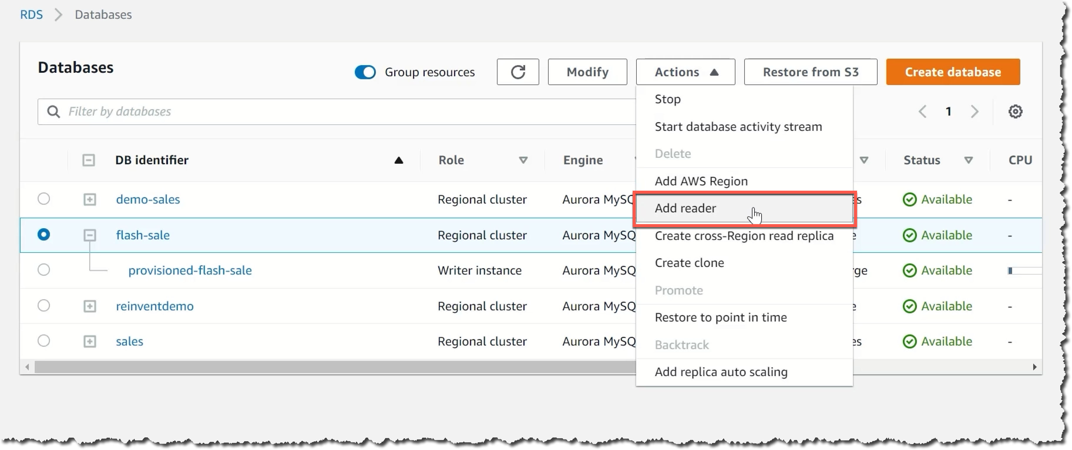
If you already have an Amazon Aurora cluster and you want to try Aurora Serverless v2, the fastest way to get started is by using mixed configuration clusters that contain both serverless and provisioned instances. Start by adding a new reader into the existing cluster. Configure the reader instance to be of the type Serverless v2.
Test the new serverless instance with your workload. Once you have confirmation that it works as expected, you can start a failover to the serverless instance, which will take less than 30 seconds to finish. This option provides a minimal downtime experience to get started with Aurora Serverless v2.

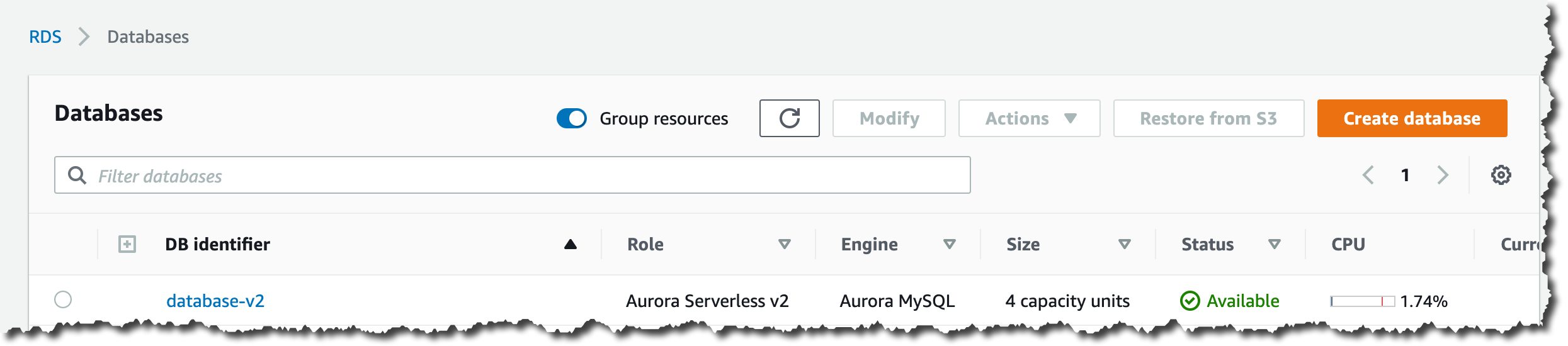
How to create a new Aurora Serverless v2 database
To get started with Aurora Serverless v2, create a new database from the RDS console. The first step is to pick the engine type: Amazon Aurora. Then, pick which database engine you want it to be compatible with: MySQL or PostgreSQL. Open the filters under Engine version and select the filter Show versions that support Serverless v2. Then, you see that the Available versions dropdown list only shows options that are supported by Aurora Serverless v2.

Next, you need to set up the database. Specify credential settings with a username and password for the administrator of the database.

Then, configure the instance for the database. You need to select what kind of instance class you want. This allocates the computational, network, and memory capacity for the database instance. Select Serverless.
Then, you need to define the capacity range. Aurora Serverless v2 capacity scales up and down within the minimum and maximum configuration. Here you can specify the minimum and maximum database capacity for your workload. The minimum capacity you can specify is 0.5 ACUs, and the maximum is 128 ACUs. For more information on Aurora Serverless v2 capacity units, see the Instant autoscaling documentation.

Next, configure connectivity by creating a new VPC and security group or use the default. Finally, select Create database.

Creating the database takes a couple of minutes. You know your database is ready when the status switches to Available.
You will find the connection details for the database on the database page. The endpoint and the port, combined with the user name and password for the administrator, are all you need to connect to your new Aurora Serverless v2 database.

Available Now!
Aurora Serverless v2 is available now in US East (Ohio), US East (N. Virginia), US West (N. California), US West (Oregon), Asia Pacific (Hong Kong), Asia Pacific (Mumbai), Asia Pacific (Seoul), Asia Pacific (Singapore), Asia Pacific (Sydney), Asia Pacific (Tokyo), Canada (Central), Europe (Frankfurt), Europe (Ireland), Europe (London), Europe (Paris), Europe (Stockholm), and South America (São Paulo).
Visit the Amazon Aurora Serverless v2 page for more information about this launch.
– Marcia
Post Syndicated from Steve Roberts original https://aws.amazon.com/blogs/aws/announcing-the-general-availability-of-aws-amplify-studio/
Amplify Studio is a visual interface that simplifies front- and backend development for web and mobile applications. We released it as a preview during AWS re:Invent 2021, and today, I’m happy to announce that it is now generally available (GA). A key feature of Amplify Studio is integration with Figma, helping designers and front-end developers to work collaboratively on design and development tasks. To stay in sync as designs change, developers simply pull the new component designs from Figma into their application in Amplify Studio. The GA version of Amplify Studio also includes some new features such as support for UI event handlers, component theming, and improvements in how you can extend and customize generated components from code.
You may be familiar with AWS Amplify, a set of tools and features to help developers get started faster with configuring various AWS services to support their backend use cases such as user authentication, real-time data, AI/ML, and file storage. Amplify Studio extends this ease of configuration to front-end developers, who can use it to work with prebuilt and custom rich user interface (UI) components for those applications. Backend developers can also make use of Amplify Studio to continue development and configuration of the application’s backend services.
Amplify Studio’s point-and-click visual environment enables front-end developers to quickly and easily compose user interfaces from a library of prebuilt and custom UI components. Components are themeable, enabling you to override Amplify Studio‘s default themes to customize components according to your own or your company’s style guides. Components can also be bound to backend services with no cloud or AWS expertise.
Support for developing the front- and backend tiers of an application isn’t all that’s available. From within Amplify Studio, developers can also take advantage of AWS Amplify Hosting services, Amplify‘s fully managed CI/CD and hosting service for scalable web apps. This service offers a zero-configuration way to deploy the application by simply connecting a Git repository with a built-in continuous integration and deployment workflow. Deployment artifacts can be exported to tools such as the AWS Cloud Development Kit (AWS CDK), making it easy to add support for other AWS services unavailable directly within Amplify Studio. In fact, all of the artifacts that are created in Amplify Studio can be exported as code for you to edit in the IDE of your choice.
You can read all about the original preview, and walk through an example of using Amplify Studio and Figma together, in this blog post published during re:Invent.
UI Event Handlers
Front-end developers are likely familiar with the concepts behind binding events on UI components to invoke some action. For example, selecting a button might cause a transition to another screen or populate some other field with data, potentially supplied from a backend service. In the following screenshot, we’re configuring an event handler for the onClick event on a Card component to open a new browser tab:
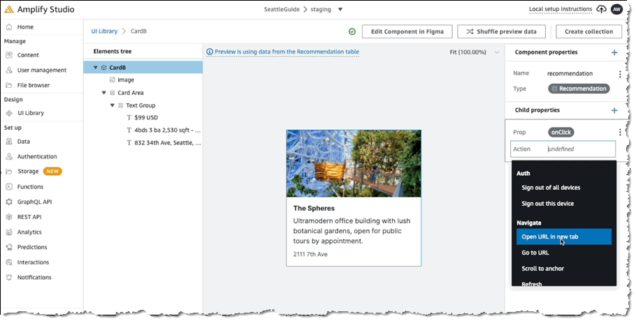
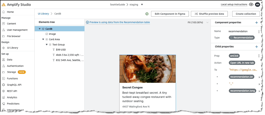
For the selected action we then define the settings, in this case to open a map view onto the location using the latitude and longitude in the card object’s model:
Extending Components with Code
When you pull your component designs from Figma into your project in Amplify Studio using the amplify pull command, generated JSX code and TypeScript definition files that map to the Figma designs are added to your project. While you could then edit the generated code, the next time you run the pull command, your changes would be overwritten.
Instead of requiring you to edit the generated code, Amplify Studio exposes mechanisms that enable you to extend the generated code to achieve the changes you need without risking losing those changes if the component code files get regenerated. While this was possible in the original preview, the GA version of Amplify Studio makes this process much simpler and more convenient. There are four ways to change generated components within Amplify Studio:
Collection type, and we want to control how (or even if) the items in the collection wrap when rendered. The Collection type exposes a wrap property which we can make use of:
<MyCustomCollection wrap={"nowrap"} />overrides prop. This prop enables you to supply an object containing multiple prop overrides, giving you full control over extending that generated code. In the following example, I’m changing the color prop belonging to the Title prop of my collection’s items to orange. As I mentioned, the settings object I’m using could contain other properties I want to override too:
<MyCustomCollectionItem overrides={{"Title": { color: "orange" } }} />overrideItems prop. You supply a function to this property, accepting parameters for the item and the item’s index in the collection. The output from the function is a set of override props to apply to that item. In the following example, I’m toggling the background color for a collection item depending on whether the item’s index is odd or even. Note that I’m also able to attach code to the item, in this case, an onClick handler that reports the ID of the item that was clicked:
<MyCustomCollection overrideItems={({ item, index })=>({
  backgroundColor: index % 2 === 0 ? 'white' : 'lightgray',
  onClick: () = alert(`You clicked item with id: ${item.id}`)
})} />ui channel. In your listener, you inspect the received events and take action on those of interest. You identify the events using names, which have a specific format, actions:[category]:[action_name]:[status]. You can find a list of all action event names in the documentation. In the following example, I’m attaching a listener in which I want to run some custom code when a new item in a DataStore has completed creation. In my code I need to inspect, in my listener, for an event with the name actions:datastore:create:finished:
import { Hub } from 'aws-amplify'
…
Hub.listen("ui", (capsule) => {
  if (capsule.payload.event === "actions:datastore:create:finished"){
      // An object has been created, do something in response
  }
});
Component Theming
To accompany the GA release of Amplify Studio, we’ve also released a Figma plugin that allows you to match UI components to your company’s brand and style. To enable it, simply install the Theme Editor plugin from the Figma community link. For example, let’s say I wanted to match Amazon’s brand colors. All I’d have to do is configure the primary color to the Amazon orange (#ff9900) color, and then all components will automatically reflect that primary color.
Get Started with AWS Amplify Studio Today
Visit the AWS Amplify Studio homepage to discover more features, whether you’re a backend or front-end developer, or both! It’s free to get started and designed to help simplify not only the configuration of backend services supporting your application but also the development of your application’s front end and the connections to those backend services. If you’re new to Amplify Studio, you’ll find a tutorial on developing a React-based UI and information on connecting your application to designs in Figma in the documentation.
Post Syndicated from Channy Yun original https://aws.amazon.com/blogs/aws/aws-iot-twinmaker-is-now-generally-available/
Last year at AWS re:Invent 2021, we introduced the preview of AWS IoT TwinMaker, a new AWS IoT service that makes it faster and easier to create digital twins of real-world systems and use them to monitor and optimize industrial operations.
A digital twin is a living digital representation of an individual physical system that is dynamically updated with data to mimic the true structure, state, and behavior of the physical system in order to drive business outcomes. Digital twins can be applied to a wide variety of use cases spanning the entire lifecycle of a system or asset, such as buildings, factories, industrial equipment, and production lines.

Many of our customers are still early in their digital twins journey. They are working hard to connect their data across disparate sources and be able to contextually visualize that data in a dashboard or an immersive environment in order to unlock their business value and outcomes.
Today at AWS Summit San Francisco, we announce the general availability of AWS IoT TwinMaker with new features, improvements, and the availability in additional AWS Regions. AWS IoT TwinMaker provides the tools to build digital twins using existing data from multiple sources, create virtual representations of any physical environment, and combine existing 3D models with real-world data. With AWS IoT TwinMaker, you can now harness digital twins to create a holistic view of your operations faster and with less effort.

AWS IoT TwinMaker has capabilities for each stage of the digital twin building process: collecting data from diverse data sources using connectors (components), connecting to data where it lives to represent your digital twins, and combining existing 3D visual models with real-world data using a scene composition tool, and building web-based applications using a plug-in for Grafana and Amazon Managed Grafana that you can use to create dashboards.
For example, Cognizant’s 1Facility solution uses AWS IoT TwinMaker to help improve the building monitoring experience by reducing the time to troubleshoot a building issue via 3D visualization and aggregating data from multiple sources in a connected building. To learn about more use cases, visit AWS IoT TwinMaker Customers.
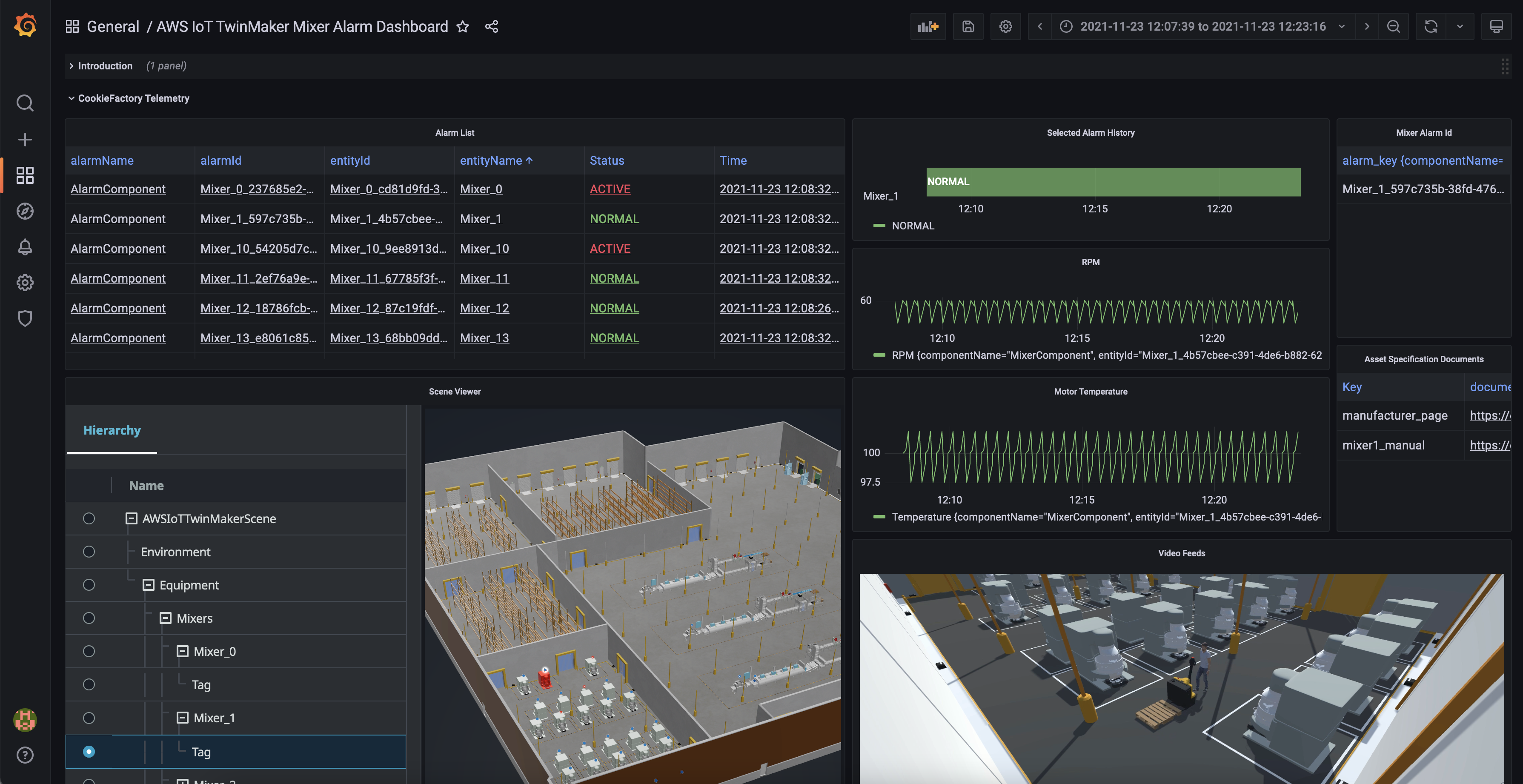
To get started with AWS IoT TwinMaker, refer to the step-by-step process for building your digital twin in Introducing AWS IoT TwinMaker. Also, you can test a fully built-out sample digital twin of a cookie factory complete with simulated data connectors from the GitHub repository. This sample code will guide you through the process of building a digital twin application and let you explore many of the features of AWS IoT TwinMaker.
New Features at the General Availability Launch
At this launch, we added some new features in AWS IoT TwinMaker:
Motion indicator – In preview, developers choose from two ways to represent data in a 3D scene: 1) tag, which can be used to bind an entity with a property and use simple rules to drive behavior like changing colors in near real time when certain conditions are met, and 2) model shader, used to change the color of the entire entity based on simple rules. Now there is a third option, motion indicator, to depict speed of motion in addition to tags (alerts) and color overlay (changing a model’s color).
There are three kinds of motion indicators for different use cases with different visuals, for example, LinearPlane (for conveyor belt), LinearCylinder (for tube), and CircularCylinder (for mixer). You can configure the motion speed and the background or foreground color of the indicator widget with either static values or with rules that will change according to different data input.
Scene templatization – With this new feature, all the data bindings such as for tags and model shaders are templatized. You can choose a template for the data binding in the console. For example, a tag can bind to each ${entityId}/${componentName}/AlarmStatus. When the operator selects the alarm for Mixer 1, the Mixer 3D Scene shows the information for Mixer 1; if the operator chooses Mixer 2, then the Mixer 3D Scene will show the information for Mixer 2.
More API improvements – We are making continuous improvements to user experience across the service based on usability feedback, including in AWS IoT TwinMaker APIs. Here are some API changes:
ExternalId filter – Added a new filter to ListEntities API to allow filtering by a property that is marked as isExternalId.CREATE update type – Added new property update type CREATE to let users explicitly state the intent of the update in an entity. Previously, there were only UPDATE and DELETE.More code samples – You can refer to more developer samples to get started with AWS IoT TwinMaker. These code packages, including new data connectors such as Snowflake, are distributed through our GitHub repository for the most common scenarios, with a goal to support and build a community of developers building digital twins with AWS IoT TwinMaker.
Now Available
AWS IoT TwinMaker is available in US East (N. Virginia), US West (Oregon), Europe (Ireland), and Asia Pacific (Singapore) Regions. Now, it is also available in Europe (Frankfurt) and Asia Pacific (Sydney) Regions.
As part of the AWS Free Tier, you can use up to 50 million data access API calls for free each month for your first 12 months using AWS. When your free usage expires, or if your application use exceeds the free tier, you simply pay the rates listed on the pricing page. To learn more about AWS IoT TwinMaker, refer to the product page and the documentation.
If you are looking for an AWS IoT TwinMaker partner to support your digital twin journey, visit the AWS IoT TwinMaker Partners page. Please send feedback to AWS re:Post for AWS IoT TwinMaker or through your usual AWS support contacts.
– Channy
Post Syndicated from Carlos Martín Nieto original https://github.blog/2022-04-21-improving-git-push-times-through-faster-server-side-hooks/
At GitHub, we relentlessly pursue performance. Join me now for the tale of how we dropped a P99 time by 95% on code that runs for every single Git push operation.
Every time you push to GitHub, we run a set of checks to validate your push before accepting it. If you ever tried to push an object larger than 100MB, you are already familiar with them, as these pre-receive hooks contain that logic. Similarly, they do other checks, such as verifying that LFS objects have been successfully uploaded. These hooks help keep our servers healthy and improve the user experience.
We recently rewrote these hooks from their original Ruby implementation into Go. This rewrite was something we had in mind for a while, but what really sold us on the effort was the potential performance improvement.
Today, we’ll talk about the history of these hooks, how we discovered that the performance was problematic, and how we went about safely replacing them.
We created the first hook in 2013 to warn users that a repository was renamed. The only action was a database check for a previous name and to send a warning to the user to update their remote URL. At the time, almost all of GitHub was part of one Ruby on Rails application, so it was the logical choice for hooks as well. As time passed, more and more functionality was added to the hooks, requiring additional configuration, exception reporting, and logging.
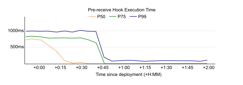
This meant that hooks imported the same dependencies as the Ruby application. Over time, the number of dependencies, and therefore startup time, only increased. In a Rails application, these dependencies are loaded only once at startup time, and then each request has them available, making the startup time not important for the user experience. However, these hooks are run as subprocesses underneath the Git executable, so they are loaded for each request, making the startup time critical to performance. When we investigated, loading these dependencies took a rather long time. Hooks took about 880 milliseconds to execute on average, and almost all of that time was spent loading dependencies. In addition, there are two sets of hooks: one with the new data under quarantine and a second set once the data is available in the repository. Especially with this double execution, this startup time significantly affects each push. An empty push could take more than two seconds, which was unacceptable.
Since the performance issues were related to startup time, we had a few options. We could reduce the number of dependencies, we could change the architecture so that hooks only started up once, or we could rewrite the hooks to run independently of the monolith. Rewrites and changing the architecture carry risk, so we tried the simplest alternative first.
Loading fewer dependencies while staying within the Rails monolith proved quite tricky. There were a lot of dependencies (more than 450 gems leading to over 1,000 require calls), and they were all quite tangled up in the app’s configuration, because they were not designed to be used outside of the GitHub Rails monolith. However, careful use of the debugger and strace revealed a few outliers that we could avoid loading when running the hooks. This removal dropped 350-400 milliseconds from the startup time.
While this was already a decent improvement for a small tweak, the startup time was still quite slow, and we weren’t satisfied yet. Additionally, new dependencies are frequently added to the Rails application, which means that the startup time would creep up again over time even if our hook code did not change.
We could not ignore the configuration from the Rails app as that is how we know how to connect to the database, send stats, etc. Some of that could be duplicated at the risk of having two parallel configuration paths that would almost certainly end up diverging.
To pass configuration along that only the app knows about, we were able to use an existing mechanism, which was already in use to pass along information, such as the name of a repository and whether it is over its quota. This comes alongside other information necessary to perform updates so it gets called for every push, and adding some more data there adds very little overhead. We identified the information necessary to perform the checks and added this information.
For the past few years, the Git Systems Team has been extracting more and more of our service code from the Rails monolith and rewriting it as a dedicated service written in Go. Based on this experience with Go, and given what we learned about the Ruby hooks, moving the hooks into this Go service seemed like a natural fit as well. Just extracting the hooks to run independently of the Rails apps would have removed most of the boot time, but Go gives us the last few milliseconds and lets us make them part of the service in which the backend code increasingly lives. We expected such a significant rewrite to be worth the risk, because afterwards the hooks should be much faster.
Further, as we commonly do for high-impact changes, we put these rewritten hooks behind a feature flag. This gave us the ability to enable them for individual repositories or groups of them. We started with a few internal GitHub repositories to confirm the effect in production.
The results were so impressive that we had to double check that the hooks were still running. It was hard to distinguish between really fast hooks and completely disabled hooks. The median time was now 10ms, compared to roughly 880ms when we started the project. This made pushes noticeably faster for everyone. We even got unprompted questions about whether pushing had become faster after someone noticed it on their own.
This is a project we had in mind for a long time. We had wanted to rewrite these hooks outside of the monolith to separate our area of responsibility better. However, merely having a better architecture often isn’t enough to make something a business priority. By tying the change to its impact on users we could prioritize this work. We came away with the dual benefits of a much better user experience and an architectural improvement.
This change has now been live on github.com for a couple of months, and has been shipped in GHES 3.4, so everyone now saves some time pushing to their GitHub repositories.
Post Syndicated from original https://lwn.net/Articles/892226/
The Debian project leader election has completed and Jonathan Carter has been reelected for his third term. For more information, see the Debian vote page. We looked at the candidates back in March.
Post Syndicated from Matt Granger original https://www.youtube.com/watch?v=V0x6buNL6hA
Post Syndicated from Molly Clancy original https://www.backblaze.com/blog/how-a-national-nonprofit-protects-field-staff-workstations/
Saving the environment is one of the most noble tasks anyone can undertake, but the thing about the environment is that it’s notoriously rough on laptops.
For the staff of The Wilderness Society, saving wild places means trekking out into said wild with boots firmly on the ground. Whether that means shutting down copper mines that would have otherwise devastated nearby waterways or helping create public transportation routes out to public lands, The Wilderness Society is a group constantly on the move. That doesn’t leave a lot of time for dealing with backups, particularly in the geographically far-flung areas in which The Wilderness Society researchers find themselves.
Data saved on staff laptops was regularly at risk, and The Wilderness Society needed a way to protect that data from threats both natural and otherwise. Director of Information Technology, Kristin Iden, shared how she:

Since 1935, The Wilderness Society has led the effort to permanently protect 109 million acres of wilderness in 44 states. They have been at the forefront of nearly every major public lands victory. Initiatives include climate change solutions, land and water conservation, and community-led conservation.
The urgency to put a solid workstation backup plan in place hit home for Kristin when her laptop was destroyed by a lightning strike. And yes, she’s aware of the irony. The IT director, one of the few who isn’t dragging their laptop across creation, is the one who lost data to natural disaster.
The Wilderness Society’s researchers find themselves all over the world as part of their mission to protect the environment. There are 14 offices from coast to coast, from Hallowell, Maine to Anchorage, Alaska. According to Kristin, “drop and destroy” events are not uncommon out in the field, whether it’s a laptop taking an accidental trip down a mountainside or into the waters of the Arctic Circle.
Add to that, as a nonprofit organization, The Wilderness Society always has to look at the bottom line. Their funding comes entirely from donors and sponsors, gifted with a purpose, and as much of it should go toward the mission as possible. In fact, Kristin had originally sought out a backup solution solely for executives as a way to save budget, but Backblaze’s affordability made it a no-brainer to extend backups out into the field.
“If somebody in the Arctic Circle drops and breaks their laptop, now I can get them back up and running within a couple of days. ”
—Kristin Iden, Director of Information Technology, The Wilderness Society

Kristin started with a beta test group of around 10% of the users, making sure to include a mix of field researchers, administrative workers, and executives. One important group to include in this mix was the handful of workers in truly remote regions of the country that have metered bandwidth. This obviously made regular backups difficult, but Kristin found a workaround by having them run the backup during weekly office visits.
The two members of the IT department are the sole administrators on the roughly 160 machines throughout the organization, an 80/20 mix of PC and Mac users. As such, they were able to roll out installation of Backblaze through Microsoft Intune, a mass deployment tool. The initial beta test went off without a hitch, and they took a phased approach to the remaining rollout—Backblaze was installed across the entire organization in groups of 30.

Kristin knew there was simply no way to prevent the inevitable destruction of user laptops out in the field. By focusing her efforts on finding the right backup solution, she was able to easily roll out to the entire organization a solution that protected their data from the rigors of nature.
Of paramount importance was simplifying the entire process for the users. They are, after all, doing the truly critical work of protecting the environment. Whether that means surveying wildlife in their native environment or working with lawmakers to craft bills that preserve nature, Kristin wanted their focus on the mission and not on their machine. With a lightweight client that doesn’t bog down machines and reliable backups she can use to provision new machines and recover data, Backblaze gave her that turnkey solution, and the peace of mind that followed.
“Admin tasks like backups are a time suck when you’re a two-person team minding 160 people running around the country trying to make sure the forests stay up. I don’t have time to babysit something constantly. With Backblaze, it just does its thing, and it lets me know when something’s not working. That’s exactly what I want out of every tool I use—just work, tell me when it isn’t, and make it easy to fix it. Backblaze just works everywhere we need it to.”
—Kristin Iden, Director of Information Technology, The Wilderness Society
Looking for a backup solution for your nonprofit organization or dispersed field staff? Learn more about Backblaze Business Backup for workstations.
The post How a National Nonprofit Protects Field Staff Workstations appeared first on Backblaze Blog | Cloud Storage & Cloud Backup.
Post Syndicated from Bria Grangard original https://blog.rapid7.com/2022/04/21/rapid7-named-a-visionary-in-2022-magic-quadrant-for-application-security-testing-second-year-in-a-row/

For the second year in a row, Rapid7 has been named a Visionary in the Gartner® 2022 Magic Quadrant for Application Security Testing. We believe we accomplished this by combining an industry-leading dynamic application security testing (DAST) solution with container and cloud security, security across the software development life cycle (SDLC), strategic partnerships, and a customer-centric approach that anticipates the needs of not just security teams but DevOps teams as well. All in a package that is easy to utilize and highly accurate.
We are proud of the approach we have taken to keeping applications and APIs safe and secure. We recognized early that while DAST is the bedrock of a strong application security program, it works best when combined with the core capabilities we have built into our platform that allow for teams across the company to work together, rather than be siloed and inefficient.
We offer support for developer stakeholders across the SDLC (pre- and post-production), actively moving left in the lifecycle, and ensuring that applications and APIs are secure throughout the development process. This means teams can work cross-functionally, saving time and resulting in stronger security protections baked into the applications themselves. Our Attack Replay feature allows developers to confirm a vulnerability on their own, without the need to run a scan, making it even easier to find and remediate risks at any point in the process.
“The product provides our developers with actionable solutions to security risks that was missed during development.”
– Infosec analyst via Gartner Peer Insights
At Rapid7, we are very proud of our history of innovative, modern, and forward-thinking vulnerability management solutions. However, it takes more than that to secure modern web applications. InsightAppSec integrates with the Insight platform, giving you a full view of your production environment. We have made a series of strategic investments and partnerships to expand the level and competency of our Insight platform, including those with Snyk and Checkmarx, which ensure that InsightAppSec is prepared to cover every level of your attack surface from every angle.
Our focus on cloud-native applications, in particular, means we have the tools to protect the most cutting-edge applications and to help those transitioning into the cloud — all with the ease and confidence that comes from our customer-centric approach to application security.
“In my opinion InsightAppSec approaches DAST the optimal way, with a cloud-based interface and the ability to spin up on-premises engines to perform scans. This means we’re not responsible for software updates, and the on-premises engines have an auto-update functionality that make them very low maintenance.”
– Sr. Software Security Engineer, IT Services via Gartner Peer Insights
At the heart of our capabilities is our world-class DAST. It’s powerful, it’s accurate, it’s streamlined, and it’s cloud-based. This allows for security teams to spin up scans quickly and easily. We frequently hear from customers that we provide the most reliable results. Our Universal Translator allows coverage and attacks to be developed in parallel and released to customers as they are available, and it lets users perform security testing for traditional applications and modern applications.
“Our experience with Rapid7 products has always been positive. InsightAppSec is a great solution for DAST scanning of web apps and API. It gives great results even in unauthenticated scans and has a great UI.”
– Cybersecurity Architect, Banking Industry via Gartner Peer Insights
We are truly excited to be recognized as a Visionary in the latest Magic Quadrant, but we’re more excited for the many plans we have to improve and grow our AppSec offerings. We have always sought to redefine what modern application security looks like and are grateful to our customers and partners for taking this exciting journey with us.
Source: Gartner, Magic Quadrant for Application Security Testing, Dale Gardner, Mark Horvath, Dionisio Zumerle, 18th April
Gartner and Magic Quadrant are registered trademarks of Gartner, Inc. and/or its affiliates in the U.S. and internationally and are used herein with permission. All rights reserved.
Gartner does not endorse any vendor, product or service depicted in its research publications and does not advise technology users to select only those vendors with the highest ratings or other designation. Gartner research publications consist of the opinions of Gartner’s Research & Advisory organization and should not be construed as statements of fact. Gartner disclaims all warranties, expressed or implied, with respect to this research, including any warranties of merchantability or fitness for a particular purpose.
Post Syndicated from Marcia Villalba original https://aws.amazon.com/blogs/aws/automatically-detect-operational-issues-in-lambda-functions-with-amazon-devops-guru-for-serverless/
Today we are announcing Amazon DevOps Guru for Serverless, a new capability for Amazon DevOps Guru. It allows developers to improve the operational performance and availability of serverless applications.
AWS pioneered the serverless computing space with the launch of AWS Lambda in 2014. Today, hundreds of thousands of customers are using AWS Lambda. Lambda allows you to configure many parameters for your functions, like memory allocation, provisioned concurrency, and timeouts. For many customers, finding the right balance between all those parameters to optimize the performance and availability of their functions is challenging.
In December 2020, we announced DevOps Guru, a fully managed AIOps (Artificial Intelligence for IT operations) service that automatically detects and alerts customers about application issues and helps them to improve their applications’ availability. Today, we are announcing DevOps Guru for Serverless, a new capability for DevOps Guru, to help developers using Lambda automatically detect anomalous behavior at the function level and use ML-powered recommendations to remediate any issues that were detected.
DevOps Guru for Serverless uses ML to automatically identify and analyze a wide range of performance and availability-related issues for Lambda functions, such as low provisioned concurrency or underutilization of memory. To use this capability, you don’t need to be a serverless or ML expert.
The reactive insights of this capability help you troubleshoot ongoing issues affecting serverless applications efficiently with actionable recommendations that help you identify and fix the root cause in the shortest time possible.
DevOps Guru for Serverless also provides proactive insights that help you identify a wider range of operational anomalies long before your serverless application performance is affected. It also gives you recommendations on how to resolve the root cause of the issues.
When an issue is detected, DevOps Guru for Serverless displays the finding in the DevOps Guru console and sends notifications using Amazon EventBridge or Amazon Simple Notification Service (Amazon SNS). This allows developers to automatically manage and take real-time action on the discovered issues.
DevOps Guru for Serverless Proactive Insights
DevOps Guru for Serverless enables developers to proactively detect application issues before an event that affects the customer occurs. For example, if provision concurrency is set too low for a Lambda function and traffic for this application is growing, DevOps Guru will detect the growing traffic and the application latency degradation and generate a proactive insight showing the issue.
ML algorithms create these insights from operational data and application metrics. An insight provides high-level information, severity, status, and a recommendation for how to solve this issue.
Nowadays, DevOps Guru for Serverless provides proactive insights for Lambda and Amazon DynamoDB. These are the operational issues and the proactive insights available today:
Get started with DevOps Guru for Serverless
To get started, navigate to the DevOps Guru console to enable the service for your Lambda-based applications, other supported resources, or your entire account.

For this demo, create a new Lambda function with provisioned concurrency of 1. You can do this from the AWS console or programmatically. After you create it, you can check on the function overview page that the provisioned concurrency is set to 1.

Add to the Lambda function a CloudWatch Event that triggers the function every minute. You can do that from the AWS console or programmatically. You can follow this tutorial to learn how to do it. Repeat that process five more times. Now the function will get triggered six times every minute from different events.
To trigger the proactive insight, you need to have six concurrent invocations of this Lambda function. To accomplish that, you need to ensure that the duration of each invocation is long enough. For this demo, you can make your function sleep for 30 seconds.
'use strict';

exports.handler = async (event) => {

    console.log('Sleep for 30 seconds')
    await new Promise(r => setTimeout(r, 30000));
    console.log('finish sleeping')

    return;
};
This configuration will trigger the proactive insight Lambda Provisioned Concurrency function limit breached for this function. You should see the insight in the console in three hours or less after the issue starts.
How to Check an Insight From the DevOps Guru Console
After a few hours, you can visit your DevOps Guru console, and you can verify that the proactive insight was triggered by exceeding the provisioned concurrency.

Select the Ongoing insight to see more details. The insight page opens, and it displays information relevant to the insight, metrics, events, and recommended actions for this issue.
Let’s examine this page in more detail. At the top of the page is the insight overview, with a description of what the insight is about and the severity of the issue. This is a proactive insight, so the user experience is not compromised by this issue. You also learn if the issue is ongoing and when it started. If the issue is not happening anymore, you can learn the end date for that insight. If you select the link for the affected applications, you can confirm all the Lambda functions that are affected by this insight.

The next information box contains information about the CloudWatch metrics related to the proactive insight. This graph shows the metric ProvisionedConcurrecySpilloverInvocations with the summary of all the invocations in the last hours that the provisioned concurrency spilled.

Relevant events are the next information box available on the page. These are AWS CloudTrail events that DevOps Guru uses combined with CloudWatch metrics and operational data to identify anomalous behavior that created the insight.

And finally on the page is the Recommendations information box, where DevOps Guru will output all the generated recommendations to help you address the issue. You can use the recommendations to learn the immediate steps you can take to remediate the issue.
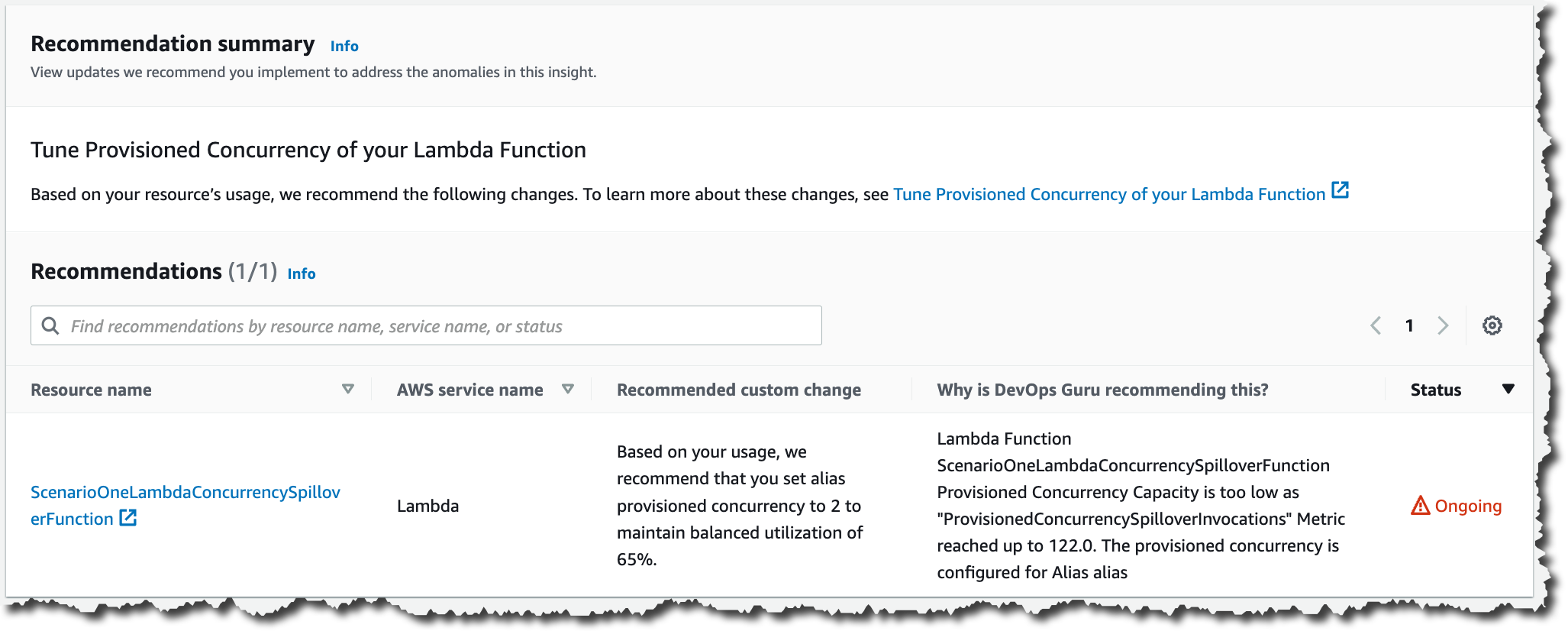
In this proactive insight, DevOps Guru recommends you tune the provision concurrency of your Lambda function. It tells you to which value to set it, based on the past utilization of your function. You can also find the reasoning on why DevOps Guru recommends this insight.
Pricing and Availability
DevOps Guru for Serverless is offered to customers at no additional charge.
DevOps Guru for Serverless is available in all AWS Regions where DevOps Guru is available, US East (Ohio), US East (N. Virginia), US West (Oregon), Asia Pacific (Singapore), Asia Pacific (Sydney), Asia Pacific (Tokyo), Europe (Frankfurt), Europe (Ireland), and Europe (Stockholm).
Learn more about DevOps Guru for Serverless and register for the hands-on workshop on May 10 to learn more about this new launch.
— Marcia
Post Syndicated from original https://lwn.net/Articles/890272/
The world of music and audio production is largely dominated by
proprietary software vendors. Among them, Steinberg stands out as a company
that created some of the most-used software, including the Cubase and Nuendo digital audio
workstations. Steinberg is also known as the creator of the VST plugin API
that, largely due to its licensing policy, has irritated developers enough to
inspire multiple attempts at creating an open-source alternative. Even now,
when the VST3 SDK is available under the
GPLv3 license, the way the company exercises its control over the SDK
keeps pushing developers away toward other open-source solutions.
This is an introduction to open-source plugin
APIs for musicians and sound engineers alike. It focuses on the options in
the larger ecosystem and how their shortcomings led to the creation of new
alternatives with liberal licensing.
Post Syndicated from original https://lwn.net/Articles/892214/
Security updates have been issued by Fedora (frr, grafana, gzip, and pdns), Oracle (java-11-openjdk), Red Hat (java-11-openjdk and kernel), Scientific Linux (java-11-openjdk), SUSE (dcraw, GraphicsMagick, gzip, kernel, nbd, netty, qemu, SDL, and xen), and Ubuntu (libinput, linux, linux-aws, linux-aws-5.13, linux-azure, linux-azure-5.13, linux-gcp, linux-gcp-5.13, linux-hwe-5.13, linux-kvm, linux-oracle, linux-oracle-5.13, linux-raspi, linux, linux-aws, linux-aws-hwe, linux-azure, linux-azure-4.15, linux-dell300x, linux-gcp, inux-gcp-4.15, linux-hwe, linux-kvm, linux-oracle, linux-snapdragon, linux, linux-aws, linux-azure, linux-azure-5.4, linux-azure-fde, linux-gcp, linux-gcp-5.4, linux-gke, linux-gke-5.4, linux-gkeop, linux-gkeop-5.4, linux-hwe-5.4, linux-ibm, linux-ibm-5.4, linux-kvm, linux-oracle, linux-oracle-5.4, linux-raspi, linux-raspi-5.4, and linux-oem-5.14).
Post Syndicated from Николай Марченко original https://bivol.bg/%D0%BC%D0%B8%D0%BD%D0%B8%D1%81%D1%82%D1%8A%D1%80%D1%8A%D1%82-%D0%BD%D0%B0-%D1%82%D1%80%D0%B0%D0%BD%D1%81%D0%BF%D0%BE%D1%80%D1%82%D0%B0-%D1%81%D0%B8-%D1%83%D1%80%D0%B5%D0%B4%D0%B8-%D0%BF%D1%80%D0%B5.html

Министърът на транспорта и съобщенията Николай Събев е злоупотребил със служебното положение, показа проверката на „Биволъ“ за личния му автомобил. Преди около месец личният му джип Mercedes–Benz GLE63AMG е включен…
Post Syndicated from original https://lwn.net/Articles/892161/
The OpenWrt 21.02.3
and 19.07.10
updates have been released. These updates contain some security fixes and
improved device support. It’s noting that this is the last 19.07 update:
OpenWrt 19.07.10 is the final release of the 19.07 release branch,
this branch is now end of life and we will not fix problems on this
branch any more, not even severe security problems. We encourage
all users still using OpenWrt 19.07 to upgrade to OpenWrt 21.02 or
more recent OpenWrt versions.
Router distributions are easy to forget about; now might be a good time to
check any relevant systems and, if needed, doing in upgrade.