Vanilla OS, a lightweight,
immutable operating system designed for developers and advanced users, has
been using Ubuntu as its base. However, a
recent announcement
has revealed that, in the upcoming Vanilla OS 2.0 Orchid release, the
project will be shifting to Debian unstable (Sid) as
its new base
operating system. Vanilla OS is making the switch due to Ubuntu’s changes to
its version of the GNOME desktop environment along with the distribution’s
reliance on the Snap packaging format.
The decision has generated a fair amount of interest and
discussion within the open-source community.
Data mesh is a new approach to data management. Companies across industries are using a data mesh to decentralize data management to improve data agility and get value from data. However, when a data producer shares data products on a data mesh self-serve web portal, it’s neither intuitive nor easy for a data consumer to know which data products they can join to create new insights. This is especially true in a large enterprise with thousands of data products.
This post shows how to use machine learning (ML) and Amazon Neptune to create automated recommendations to join data products and display those recommendations alongside the existing data products. This allows data consumers to easily identify new datasets and provides agility and innovation without spending hours doing analysis and research.
Background
The success of a data-driven organization recognizes data as a key enabler to increase and sustain innovation. It follows what is called a distributed system architecture. The goal of a data product is to solve the long-standing issue of data silos and data quality. Independent data products often only have value if you can connect them, join them, and correlate them to create a higher order data product that creates additional insights. A modern data architecture is critical in order to become a data-driven organization. It allows stakeholders to manage and work with data products across the organization, enhancing the pace and scale of innovation.
Solution overview
A data mesh architecture starts to solve for the decoupled architecture by decoupling the data infrastructure from the application infrastructure, which is a common challenge in traditional data architectures. It focuses on decentralized ownership, domain design, data products, and self-serve data infrastructure. This allows for a new way of thinking and new organizational elements—namely, a modern data community.
However, today’s data mesh platform contains largely independent data products. Even with well-documented data products, knowing how to connect or join data products is a time-consuming job. Data consumers spend hours, days, or months to understand and analyze the data. Identifying links or relationships between data products is critical to create value from the data mesh and enable a data-driven organization.
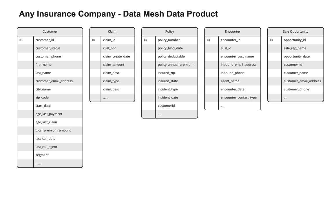
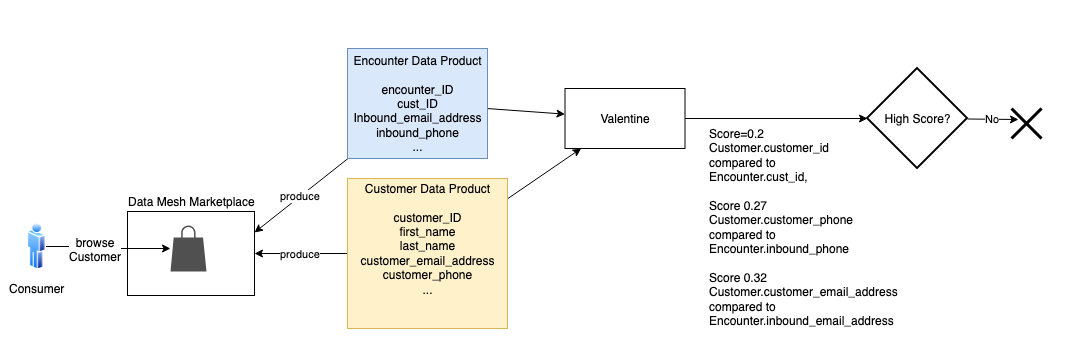
The solution in this post illustrates an approach to solving these challenges. It uses a fictional insurance company with several data products shared on their data mesh marketplace. The following figure shows the sample data products used in our solution.
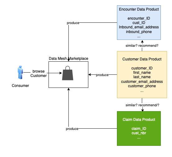
Suppose a consumer is browsing the customer data product in the data mesh marketplace. The consumer wonders if the customer data could be linked to claim, policy, or encounter data. Because these data products come from different lines of business (LOBs) or silos, it’s hard to know. A consumer would have to review each data product and do the necessary analysis and research to know this with any certainty.
To solve this problem, our solution uses ML and Neptune to create recommendations for the data consumer. The solution generates a list of data products, product attributes, and the associated probability scores to show join ability. This reduces the time to discover, analyze, and create new insights.
We use Valentine, a data science algorithm for comparing datasets, to improve data product recommendations. Neptune, the managed AWS graph database service, stores information about explicit connections between datasets, improving the recommendations.
Example use case
Let’s walk through a concrete example. Suppose a consumer is browsing the Customer data product in the data mesh marketplace. Customer is similar to the Policy and Encounter data products, but these products come from different silos. Their similarity to the Customer is hard to gauge. To expedite the consumer’s work, the mesh recommends how the Policy and Encounter products can be connected to the Customer product.
Let’s consider two cases. First, is Customer similar to Claim? The following is a sample of the data in each product.
Intuitively, these two products have lots of overlap. Every Cust_Nbr in Claim has a corresponding Customer_ID in Customer. There is no foreign key constraint in Claim that assures us it points to Customer. We think there is enough similarity to infer a join relationship.
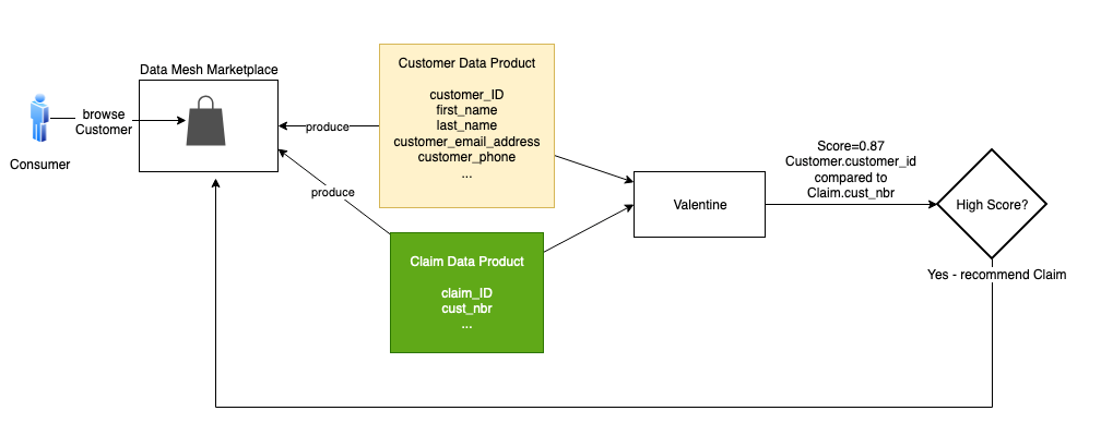
The data science algorithm Valentine is an effective tool for this. Valentine is presented in the paper Valentine: Evaluating Matching Techniques for Dataset Discovery (2021, Koutras et al.). Valentine determines if two datasets are joinable or unionable. We focus on the former. Two datasets are joinable if a record from one dataset has a link to a record in the other dataset using one or more columns. Valentine addresses the use case where data is messy: there is no foreign key constraint in place, and data doesn’t match perfectly between datasets. Valentine looks for similarities, and its findings are probabilistic. It scores its proposed matches.
This solution uses an implementation of Valentine available in the following GitHub repo. The first step is to load each data product from its source into a Pandas data frame. If the data is large, load a representative subset of it, at most a few million records. Pass the frames to the valentine_match() function and select the matching method. We use COMA, one of several methods that Valentine supports. The function’s result indicates the similarity of columns and the score. In this case, it tells us that the Customer_ID for Customer matches the Cust_Nbr for Claim, with a very high score. We then instruct the data mesh to recommend Claim to the consumer browsing Customer.
A graph database isn’t required to recommend Claim; the two products could be directly compared. But let’s consider Encounter. Is Customer similar to Encounter? This case is more complicated. Many encounters in the Encounter product don’t link to a customer. An encounter occurs when someone contacts the contact center, which could be by phone or email. The party may or may not be a customer, and if they are a customer, we may not know their customer ID during this encounter. Additionally, sometimes the phone or email they use isn’t the same as the one from a customer record in the Customer product.
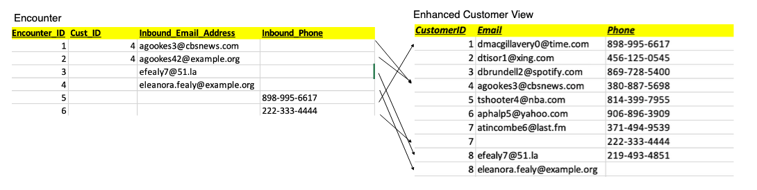
In the following sample encounter set, encounters 1 and 2 match to Customer_ID 4. Note that encounter 2’s inbound_email doesn’t exactly match the inbound_email in that customer’s record in the Customer product. Encounter 3 has no Customer_ID, but its inbound_email matches the customer with ID 8. Encounter 4 appears to refer to the customer with ID 8, but the email doesn’t match, and no Customer_ID is given. Encounter 5 only has Inbound_Phone, but that matches the customer with ID 1. Encounter 6 only has an Inbound_Phone, and it doesn’t appear to match any of the customers we’ve listed so far.
We don’t have a strong enough comparison to infer similarity.
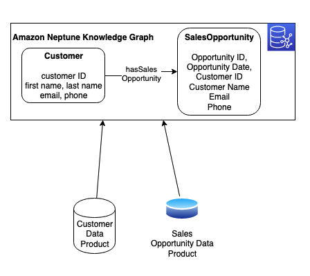
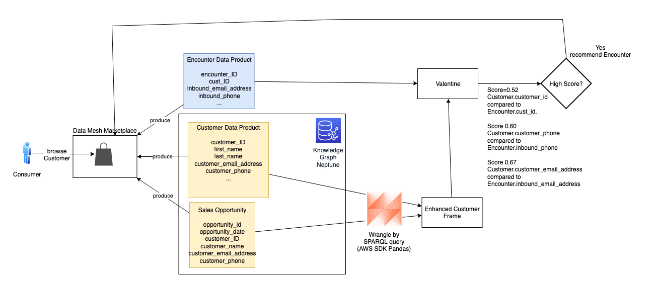
But we know more about the customer than the Customer product tells us. In the Neptune database, we maintain a knowledge graph that combines multiple products and links them through relationships. A knowledge graph allows us to combine data from different sources to gain a better understanding of a specific problem domain. In Neptune, we combine the Customer product data with an additional data product: Sales Opportunity. We ingest each product from its source into the knowledge graph and model a hasSalesOpportunity relationship between Customer and SalesOpportunity resources. The following figure shows these resources, their attributes, and their relationship.
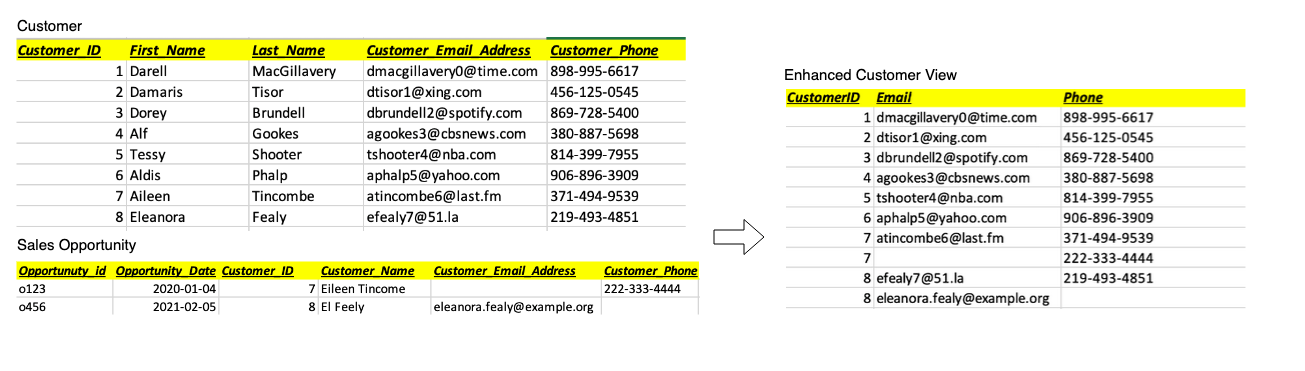
With the AWS SDK for Pandas, we combine this data by running a query against the Neptune graph. We use a graph query language (such as SPARQL) to wrangle a representative subset of customer and sales opportunity data into a Pandas data frame (shown as Enhanced Customer View in the following figure). In the following example, we enhance customers 7 and 8 with alternate phone or email contact data from sales opportunities.
We pass that frame to Valentine and compare it to Encounter. This time, two additional encounters match a customer.
The score meets our threshold, and is high enough to share with the consumer as a possible match. To the customer browsing Customer in the mesh marketplace, we present the recommendation of Encounter, along with scoring details to support the recommendation. With this recommendation, the consumer can explore the Encounter product with greater confidence.
Conclusion
Data-driven organizations are transitioning to a data product way of thinking. Utilizing strategies like data mesh generates value on a large scale. We took this a step further by creating a blueprint to create smart recommendations by linking similar data products using graph technology and ML. In this post, we showed how an organization can augment a data catalog with additional metadata by using ML and Neptune with an automated process.
This solution solves the interoperability and linkage problem for data products. Additionally, it gives organizations real-time insights, agility, and innovation without spending time on data analysis and research. This approach creates a truly connected ecosystem with simplified access to delight your data consumers. The current solution is platform agnostic; however, in a future post we will show how to implement this using data.all (open-source software) and Amazon DataZone.
Moira Lennox is a Senior Data Strategy Technical Specialist for AWS with 27 years’ experience helping companies innovate and modernize their data strategies to achieve new heights and allow for strategic decision-making. She has experience working in large enterprises and technology providers, in both business and technical roles across multiple industries, including health care live sciences, financial services, communications, digital entertainment, energy, and manufacturing.
Joel Farvault is Principal Specialist SA Analytics for AWS with 25 years’ experience working on enterprise architecture, data strategy, and analytics, mainly in the financial services industry. Joel has led data transformation projects on fraud analytics, claims automation, and data governance.
Mike Havey is a Solutions Architect for AWS with over 25 years of experience building enterprise applications. Mike is the author of two books and numerous articles. His Amazon author page
Many customers run big data workloads such as extract, transform, and load (ETL) on Apache Hive to create a data warehouse on Hadoop. Apache Hive has performed pretty well for a long time. But with advancements in infrastructure such as cloud computing and multicore machines with large RAM, Apache Spark started to gain visibility by performing better than Apache Hive.
Customers now want to migrate their Apache Hive workloads to Apache Spark in the cloud to get the benefits of optimized runtime, cost reduction through transient clusters, better scalability by decoupling the storage and compute, and flexibility. However, migration from Apache Hive to Apache Spark needs a lot of manual effort to write migration scripts and maintain different Spark job configurations.
In this post, we walk you through a solution that automates the migration from HiveQL to Spark SQL. The solution was used to migrate Hive with Oozie workloads to Spark SQL and run them on Amazon EMR for a large gaming client. You can also use this solution to develop new jobs with Spark SQL and process them on Amazon EMR. This post assumes that you have a basic understanding of Apache Spark, Hive, and Amazon EMR.
Solution overview
In our example, we use Apache Oozie, which schedules Apache Hive jobs as actions to collect and process data on a daily basis.
We migrate these Oozie workflows with Hive actions by extracting the HQL files, and dynamic and static parameters, and converting them to be Spark compliant. Manual conversion is both time consuming and error prone. To convert the HQL to Spark SQL, you’ll need to sort through existing HQLs, replace the parameters, and change the syntax for a bunch of files.
Instead, we can use automation to speed up the process of migration and reduce heavy lifting tasks, costs, and risks.
We split the solution into two primary components: generating Spark job metadata and running the SQL on Amazon EMR. The first component (metadata setup) consumes existing Hive job configurations and generates metadata such as number of parameters, number of actions (steps), and file formats. The second component consumes the generated metadata from the first component and prepares the run order of Spark SQL within a Spark session. With this solution, we support basic orchestration and scheduling with the help of AWS services like Amazon DynamoDB and Amazon Simple Storage Service (Amazon S3). We can validate the solution by running queries in Amazon Athena.
In the following sections, we walk through these components and how to use these automations in detail.
Generate Spark SQL metadata
Our batch job consists of Hive steps scheduled to run sequentially. For each step, we run HQL scripts that extract, transform, and aggregate input data into one final Hive table, which stores data in HDFS. We use the following Oozie workflow parser script, which takes the input of an existing Hive job and generates configurations artifacts needed for running SQL using PySpark.
Oozie workflow XML parser
We create a Python script to automatically parse the Oozie jobs, including workflow.xml, co-ordinator.xml, job properties, and HQL files. This script can handle many Hive actions in a workflow by organizing the metadata at the step level into separate folders. Each step includes the list of SQLs, SQL paths, and their static parameters, which are input for the solution in the next step.
The process consists of two steps:
The Python parser script takes input of the existing Oozie Hive job and its configuration files.
The script generates a metadata JSON file for each step.
The following diagram outlines these steps and shows sample output.
The Python script parses only HiveQL actions from the Oozie workflow.xml.
The Python script generates one file for each SQL statement and uses the sequence ID for file names. It doesn’t name the SQL based on the functionality of the SQL.
Run Spark SQL on Amazon EMR
After we create the SQL metadata files, we use another automation script to run them with Spark SQL on Amazon EMR. This automation script supports custom UDFs by adding JAR files to spark submit. This solution uses DynamoDB for logging the run details of SQLs for support and maintenance.
Architecture overview
The following diagram illustrates the solution architecture.
You can check on the DynamoDB console that the table dw-etl-pipelinelog is successfully created.
The log table has the following attributes.
Attributes
Type
Comments
job_run_id
String
partition_key
id
String
sort_key (UUID)
end_time
String
End time
error_description
String
Error in case of failure
expire
Number
Time to Live
sql_seq
Number
SQL sequence number
start_time
String
Start time
Status
String
Status of job
step_id
String
Job ID SQL belongs
The log table can grow quickly if there are too many jobs or if they are running frequently. We can archive them to Amazon S3 if they are no longer used or use the Time to Live feature of DynamoDB to clean up old records.
Run the first command to set the variable in case you have an existing bucket that can be reused. If not, create a S3 bucket to store the Spark SQL code, which will be run by Amazon EMR.
export s3_bucket_name=unique-code-bucket-name # Change unique-code-bucket-name to a valid bucket name
To create the source tables in the base database, run the DDLs present in the repo in the Athena query editor:
Run the ./sample_data/ddl/states_current.q file by modifying the S3 path to the bucket you created.
Run the ./sample_data/ddl/us_current.q file by modifying the S3 path to the bucket you created.
The ETL driver file implements the Spark driver logic. It can be invoked locally or on an EMR instance.
Launch an EMR cluster.
Make sure to select Use for Spark table metadata under AWS Glue Data Catalog settings.
Add the following steps to EMR cluster.
aws emr add-steps --cluster-id <<cluster id created above>> --steps 'Type=CUSTOM_JAR,Name="boto3",ActionOnFailure=CONTINUE,Jar=command-runner.jar,Args=[bash,-c,"sudo pip3 install boto3"]'
aws emr add-steps --cluster-id <<cluster id created above>> --steps 'Name="sample_oozie_job_name",Jar="command-runner.jar",Args=[spark-submit,--py-files,s3://unique-code-bucket-name-#####/framework/code.zip,s3://unique-code-bucket-name-#####/framework/etl_driver.py,--step_id,sample_oozie_job_name#step1,--job_run_id,sample_oozie_job_name#step1#2022-01-01-12-00-01,  --code_bucket=s3://unique-code-bucket-name-#####/DW,--metadata_table=dw-etl-metadata,--log_table_name=dw-etl-pipelinelog,--sql_parameters,DATE=2022-02-02::HOUR=12::code_bucket=s3://unique-code-bucket-name-#####]' # Change unique-code-bucket-name to a valid bucket name
The following table summarizes the parameters for the spark step.
The following table summarizes the script arguments.
Script Argument
Argument Description
deploy-mode
Spark deploy mode. Client/Cluster.
name <jobname>#<stepname>
Unique name for the Spark job. This can be used to identify the job on the Spark History UI.
py-files <s3 path for code>/code.zip
S3 path for the code.
<s3 path for code>/etl_driver.py
S3 path for the driver module. This is the entry point for the solution.
step_id <jobname>#<stepname>
Unique name for the step. This refers to the step_id in the metadata entered in DynamoDB.
job_run_id <random UUID>
Unique ID to identify the log entries in DynamoDB.
log_table_name <DynamoDB Log table name>
DynamoDB table for storing the job run details.
code_bucket <s3 bucket>
S3 path for the SQL files that are uploaded in the job setup.
metadata_table <DynamoDB Metadata table name>
DynamoDB table for storing the job metadata.
sql_parameters DATE=2022-07-04::HOUR=00
Any additional or dynamic parameters expected by the SQL files.
Validation
After completion of EMR step you should have data on S3 bucket for the table base.states_daily. We can validate the data by querying the table base.states_daily in Athena.
Congratulations, you have converted an Oozie Hive job to Spark and run on Amazon EMR successfully.
Solution highlights
This solution has the following benefits:
It avoids boilerplate code for any new pipeline and offers less maintenance of code
Onboarding any new pipeline only needs the metadata set up—the DynamoDB entries and SQL to be placed in the S3 path
Any common modifications or enhancements can be done at the solution level, which will be reflected across all jobs
DynamoDB metadata provides insight into all active jobs and their optimized runtime parameters
For each run, this solution persists the SQL start time, end time, and status in a log table to identify issues and analyze runtimes
It supports Spark SQL and UDF functionality. Custom UDFs can be provided externally to the spark submit command
Limitations
This method has the following limitations:
The solution only supports SQL queries on Spark
Each SQL should be a Spark action like insert, create, drop, and so on
In this post, we explained the scenario of migrating an existing Oozie job. We can use the PySpark solution independently for any new development by creating DynamoDB entries and SQL files.
Clean up
Delete all the resources created as part of this solution to avoid ongoing charges for the resources:
Stop the EMR cluster if it wasn’t a transient cluster:
aws emr terminate-clusters --cluster-ids <<cluster id created above>>
Conclusion
In this post, we presented two automated solutions: one for parsing Oozie workflows and HiveQL files to generate metadata, and a PySpark solution for running SQLs using generated metadata. We successfully implemented these solutions to migrate a Hive workload to EMR Spark for a major gaming customer and achieved about 60% effort reduction.
For a Hive with Oozie to Spark migration, these solutions help complete the code conversion quickly so you can focus on performance benchmark and testing. Developing a new pipeline is also quick—you only need to create SQL logic, test it using Spark (shell or notebook), add metadata to DynamoDB, and test via the PySpark SQL solution. Overall, you can use the solution in this post to accelerate Hive to Spark code migration.
About the authors
Vinay Kumar Khambhampati is a Lead Consultant with the AWS ProServe Team, helping customers with cloud adoption. He is passionate about big data and data analytics.
Sandeep Singh is a Lead Consultant at AWS ProServe, focused on analytics, data lake architecture, and implementation. He helps enterprise customers migrate and modernize their data lake and data warehouse using AWS services.
Amol Guldagad is a Data Analytics Consultant based in India. He has worked with customers in different industries like banking and financial services, healthcare, power and utilities, manufacturing, and retail, helping them solve complex challenges with large-scale data platforms. At AWS ProServe, he helps customers accelerate their journey to the cloud and innovate using AWS analytics services.
Съдебните атаки срещу две независими български медии – онлайн изданията “Биволъ” и Mediapool.bg са споменати в анализа на медийния пазар в България в международното изследване Project Oasis Europe. Едногодишният изследователски…
This blog post helps customers in mitigating distributed denial-of-service (DDoS) using AWS Shield Advanced, AWS WAF, and data science. We explore how to use these services along with machine learning (ML) to detect and mitigate DDoS attacks.
Bad actors conduct DDoS attacks using botnets. Through botnets, attackers look for zero-day vulnerabilities—specifically on network devices such as routers—and make these devices a part of their network. Bots speared around the world are waiting for instructions from control servers.
This post examines a real-world use case. Online payment solutions company Razorpay has a business-to-business (B2B) model where merchants invoke APIs for payments. Given the complex nature of B2B payments, the traffic patterns between small-scale merchants and large-scale merchants needs to be distinguished. This business model puts the company at risk for DDoS attacks, and here is how AWS helps them address this ongoing concern.
First, we will introduce an initial DDoS architecture approach and then how it was modified to meet specific Razorpay needs, as is possible for cross-industry client with varying requirements.
Basic DDoS recommendations
Let’s explore some out-of-the-box DDoS business solution recommendations for different resource categories:
Static websites:Amazon CloudFront is a content delivery network (CDN) service that is used to host static websites. The AWS WAF rate-limiting rule can be used to limit traffic on a CDN.
Dynamic websites: In this scenario, a standard WAF Rate Limit rule can be used on Application Load Balancer (ALB).
APIs with customer context: APIs receive these assets on behalf of other merchants (for example, an end-user places a food order from a food-delivery application, completes a payment, and the request is sent to api.razorpay.com. Razorpay understands that the end user is trying to make a payment toward the food app).
Figure 1 represents the difficulty levels and solutions for each resource category.
Figure 1. DDoS business solution resource category recommendations
DDoS response phases
We’ve discussed initial DDoS architectures, so now let’s explore the various DDoS response phases:
Phase 1– Automated inventory: Creating an automated inventory system capturing the list of APIs or websites exposed. The APIs are ranked by exposure and risk of an outage to create a list of assets that is ranked on the basis of risk.
Phase 2 – Bucketing assets into groups: Bucketing APIs and websites (static or dynamic) into groups. This phase also subgroups the assets into unauthenticated or authenticated, users and more. As we will discuss later in this post, most Razorpay APIs have a customer context requiring a multilayered defense mechanism.
Phase 3– Testing the solution: Simulating attack traffic to test the solution under different loads, origins, and more.
AWS DDoS solutions
AWS has two major out-of-the-box solutions when protecting against DDoS attacks: AWS Shield and AWS WAF.
AWS Shield has three important features for DDoS mitigation:
Alarms: Triggers an alarm when a DDoS attack is suspected, customized based on metrics such as total volume, error rates at the ALB, and response latency
Visibility: Provides top five important field values in real time, such as requesting client IPs, countries, user agents, referrer headers, and url routes to take action.
On-call support: Provides on-call support from the Shield Response team (SRT) to understand attack vectors and create AWS WAF rules based on insights.
AWS WAF has two rule types:
Blocking: Blocks requests matching expected variables, from individuals to a combination of fields such as IP, URL route, body, or country
Rate limiting: Tracks the rate of requests for each originating IP address, and triggers the rule action on IPs with rates that go over the limit. A scope-down statement can also be added to the rule, to only track and rate limit requests that match the scope-down statement. (We will soon discuss how Razorpay relies heavily on rate limiting it the AWS WAF and other microservice architecture solutions.)
Razorpay microservices protection architecture
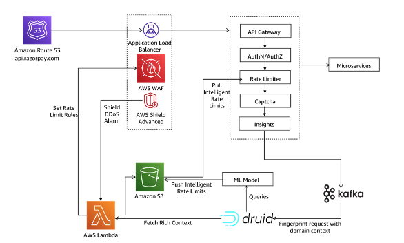
Razorpay has two main layers protecting their internal microservices. The request to payment API api.razorpay.com goes from Amazon Route 53 to ALB. AWS WAF and AWS Shield Advanced are deployed on ALB. Requests are then forwarded to microservices fronted by API Gateway as in Figure 2.
An API Gateway is a critical piece of infrastructure for microservice architectures. Razorpay is a B2B organization that performs actions on behalf of merchants. To achieve this—and understand context about the merchants and end-users alike—a custom API Gateway:
Works at a high scale with very low latency
Understands merchant context to provide authentication and authorization
Provides security features around malicious traffic
Razorpay uses a self-managed API gateway called Edge. The API Gateway is the first system on the ingress path to understand Razorpay domain context that prior layers cannot. Every request goes through multiple layers of logic at the API Gateway before being forwarded to respective services.
Razorpay Edge and AWS solution insights
As Edge performs multiple computations on each request, Razorpay generates insights for each request to build intelligence and prevent DDoS attacks. These events are fed into a time-series database in near real time and generate insights using machine learning (ML) models. The insights:
Identify malicious patterns: Generating confidence percentage that helps in defining further action, verifies consumer authenticity, and serves the request. It also blocks malicious requests at the edge.
Derive pattern-based rate limits: Deriving rate limits based on a larger set of data—including consumer and IP address—by looking at weekly and monthly patterns. Once this information is available at Razorypay Edge, it can perform various operations to ensure only legit requests reach the service layer. Let’s explore the request flow to understand each stage’s contribution toward DDoS handling, as in Figure 3.
Figure 3. Razorpay Edge request flow for DDoS handling
All Razorpay requests flow through API Gateway. Here are some key recommendations:
Based on feedback data available, the gateway checks if the given request pattern falls in the malicious category. If the confidence percentage is high for a malicious request, block the request. A block rule is applied at the AWS WAF layer. If the confidence percentage is low, use CAPTCHA to check user authenticity.
Apply rate limit on pre-existing data in the request object using feedback from an ML model.
Perform authentication/identification and authorization.
Apply rate limit on data derived from request object, also using feedback from a ML model.
Request user CAPTCHA verification if the request is identified as malicious with low confidence.
As a best practice, publish generated insights for each request to Apache Kafka out of the request flow to avoid latency impact and reduce blast radius.
Conclusion
In this post, you learned about addressing DDoS attacks with ML models.
Organizations can use the insights data generated by an API Gateway to identify request patterns, categorize the patterns into various buckets, and perform the following depending on category:
Send feedback to an API Gateway for immediate action
Update the rate limits for Edge-based historical patterns
Update WAF rule for blocking/reducing rate limits
As discussed, using AWS WAF and AWS Shield Advanced along with ML helps detect and mitigate DDoS attacks.
The desktop-oriented Solus distribution
has been through a difficult period; this post describes
the extensive changes that have been made in response.
Notably, innovation in the Linux ecosystem is presently centered
around the use of application sandboxing, containers and the
development of immutable operating systems with a well understood
Software Bill of Materials. Each of these concepts allow for a
degree of separation and stability when developing, testing and
certifying software and products.
The current Solus tooling, as well as the resulting packaging and
development experience, is somewhat ill-suited to this objective
and would most likely need a wholesale re-engineering of the tools
before this becomes feasible.
However, there is a more straightforward path for Solus: Rebasing
onto Serpent OS.
While the staffing crisis is real, our global MDR SOCs are thriving with top-notch analysts, DFIR talent, and no revolving doors (they like it here). In a high-pressure, high-stakes business, these are our lessons learned.
Measure your staffing performance meticulously and publicly
In an industry plagued by burnout, churn, and open jobs everywhere, be obsessed with your metrics to retain top talent. We do.
Last year, we grew our global Managed Detection and Response (MDR) teams by 68%
Our voluntary attrition for SOC analysts is under 5%
Since the start of Rapid7 MDR seven years ago, we’ve only lost about one to two analysts per year (as competition for cybersecurity talent went white-hot)
Rapid7 recruits talent from all over the world to join us in our state-of-the-art SOC locations. Each SOC has incredibly high retention rates.
We prioritize investments in training, competitive pay, project work and extracurricular activities, and ensuring analysts are doing the work they enjoy. The leadership team is in tune with job satisfaction and directly attacks any aspect of the analyst duties that causes friction.
Peter Drucker said it best: “Culture eats strategy for breakfast.”
According to a survey by Mimecast, 84% of security professionals are experiencing burnout due to the constant barrage of threats, the talent shortage, and other employees’ mistakes (as a result of burnout). And, while everyone battles “The Great Resignation” and our collective 5-year skills crisis, ZDNet reports it’s going to get worse. Nearly a third of the global cybersecurity workforce plans to leave the industry—not their jobs, but the entire industry—within two years.
To prevent burnout, we encourage a culture of friendship and after-hours socialization. People who work alongside friends help more and perform better. They trust one another. Like just about anyone in our line of work, Rapid7 MDR employees know they can go anywhere and do what they do. They also know we greatly appreciate the fact they choose to do it here.
A member of one of our SOC had his car in the shop for far too long due to a supply chain shortage of the missing part. There was only one thing to do for April Fool’s day:
As one member of the team stated, “we work at a place that crowdsourced a $700 prank!”
You don’t need budget for team-building consultants and “trust exercises.” Camaraderie is created in Slack channels and karaoke nights at the bar on the first floor of the Rapid7 Arlington , VA office.
Create a learning organization
We’ve heard it called “alphabet soup after your name.” While certifications are important, real-world experience and constant learning trumps a course any day of the week. And the best way for the SOC to learn? By doing first-hand and sharing those learnings with everyone. Here’s some of the lessons learned:
First, eliminate silos. Each of our MDR SOCs are composed of three tiers of analysts, working together on customer environments. There’s complete threat detection coverage, multiple layers of escalation and validation, and redundant knowledge. Additionally, the technology used by the SOC captures relevant details of the environment, detected threats, and analysis notes which are available to all analysts.
Second, train constantly. Rapid7 has a robust training program: a combination of external live training (SANS, Chris Sanders courses), self-paced learning (TCM malware analysis & forensics courses), as well as a robust internal security training program (modeled after specific incidents Rapid7 MDR has handled) to train our analysts quickly and effectively. All training is heavily focused on endpoint forensics, incident response, threat hunting, coding/scripting, and foundational security concepts. All analysts have the chance to attend external training every year. Internally, analysts learn from each other with weekly “lunch n’ learns” to level up their stills by learning from others around them and show off the latest threat they were able to thwart for our customers.
Third, we organized around learning in new ways. Over a year ago, Rapid7 merged our Incident Response Consulting Team with our MDR SOC to create an integrated team of Detection and Response experts. If an incident investigation appears to be major, analysts simply (and literally) swivel their chairs and tap Senior IR consultants and DFIR practitioners on the shoulder.
For major incidents, Rapid7’s TIDE Team (Threat Intelligence and Detections Engineering) is right there too. “We ride along with them and are watching what they’re discovering and we develop new detections,” says Eoin Miller, Manager of Detection and Response Services. “It helps not only that customer but any other customer that may be a current or future victim of that same attacker.”
Rapid7 MDR also created a “Tactical Operations” (TacOps) team, which is primarily used as a “farm system” for analyst development. Typically, Associate Analysts at other Security Operation Centers are relegated to Tier 1 roles, focusing on low severity alert triage with little exposure to actual malicious activity or complex investigations. Rapid7 takes a different approach by throwing these Associate Analysts into the deep end to deal with real, high priority threats (the things we know are evil), which accelerates their learning curve. They’re actually looking at malicious activity all day, not just hundreds of benign alerts.
Our Associate level analysts have even gone on to publish their work and were tapped to lead a technical malware deep dive on one of the most popular security webinars in the world (Ultimate IT Security). Not too shabby for “entry level” folks to be presenting to a broad audience after only a year working in our SOC. Not surprisingly, we focus on promoting from within, with many analysts taking on advanced roles in forensic analysis and IR.
Finally, we’ve reorganized our services organization to bring our penetration testing team SOC analysts under one roof. We feel the best way to learn (and improve our ability to detect and respond effectively) is to encourage collaboration and knowledge sharing between both our offensive-minded and defensive-minded security practitioners. Iron sharpens iron.
Never compromise your standards
MDR analyst candidates go through an initial technical assessment (live on phone responses) with our Talent Acquisition partners in order to pre-screen candidates before the live technical interview panel.
During the interview Technical Panel, our interviewers’ goal is to push the candidate to the edge of their knowledge. We ask a series of questions which are progressively more difficult using real-world scenarios: “If you see XYZ behavior, walk me through the process from start to finish:
What technology and methodology would you use?
What data are you looking for?
Deep dive into why and how you’re looking at it?
How do you come to the determination that the behavior is malicious or benign?
This allows us to question various tools and techniques used in the course of an investigation. We then hire based on the candidate’s knowledge, skill set, and culture fit.
Rapid7 has company core values. We’ve added to it with our “Culture Code for the MDR SOC.” Every organization and each SOC’s values are different. These are ours:
Ownership: Know what you’re responsible for and own it. We expect you to own your mission fully. Don’t make excuses, and don’t point fingers at others.
Customer-Centric: We are here for one reason—to deliver the managed security services our customers expect and deserve.
Passion and Purpose: Love what you do. While not everything you do every day is exciting, our team members genuinely enjoy their work and understand the importance of it.
Don’t Just ‘Turn The Wheel’: We’re not here just to handle alerts, run scans, perform hunts, or throw alerts over the fence for our customers to handle. We’re here to bring our security expertise to bear in the most effective way to better protect our customers at scale.
Risk Taking: Choosing not to take a risk is often the biggest risk. We will never fault someone for taking a well informed risk in order to better serve our customers.
Integrity: We never mislead customers or prospects or act against their best interests, and we are open and honest with our fellow Moose.
Never Done: This is not a clock-in / clock-out kind of job. While many days are predictable, others are not. Our North Star is customer outcomes, not time-based.
Glass Half Full: Security operations can be unforgiving—but we will remain positive and optimistic.
Have Fun: Get your job done, but have fun doing it.
We’re always looking for great security professionals to join our team. If the above piques your interest and you’re looking to join a part of something special, come check out our open Career opportunities.
When shopping for DDR4 memory modules, we typically look at the memory density and memory speed. For example a 32GB DDR4-2666 memory module has 32GB of memory density, and the data rate transfer speed is 2666 mega transfers per second (MT/s).
If we take a closer look at the selection of DDR4 memories, we will then notice that there are several other parameters to choose from. One of them is rank x organization, for example 1Rx8, 2Rx4, 2Rx8 and so on. What are these and does memory module rank and organization have an effect on DDR4 module performance?
In this blog, we will study the concepts of memory rank and organization, and how memory rank and organization affect the memory bandwidth performance by reviewing some benchmarking test results.
Memory rank
Memory rank is a term that is used to describe how many sets of DRAM chips, or devices, exist on a memory module. A set of DDR4 DRAM chips is always 64-bit wide, or 72-bit wide if ECC is supported. Within a memory rank, all chips share the address, command and control signals.
The concept of memory rank is very similar to memory bank. Memory rank is a term used to describe memory modules, which are small printed circuit boards with memory chips and other electronic components on them; and memory bank is a term used to describe memory integrated circuit chips, which are the building blocks of the memory modules.
A single-rank (1R) memory module contains one set of DRAM chips. Each set of DRAM chips is 64-bits wide, or 72-bits wide if Error Correction Code (ECC) is supported.
A dual-rank (2R) memory module is similar to having two single-rank memory modules. It contains two sets of DRAM chips, therefore doubling the capacity of a single-rank module. The two ranks are selected one at a time through a chip select signal, therefore only one rank is accessible at a time.
Likewise, a quad-rank (4R) memory module contains four sets of DRAM chips. It is similar to having two dual-rank memories on one module, and it provides the greatest capacity. There are two chip select signals needed to access one of the four ranks. Again, only one rank is accessible at a time.
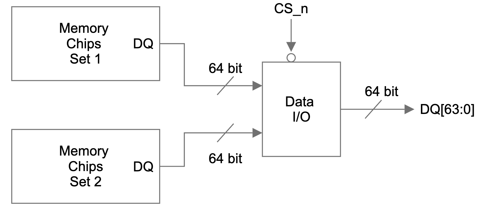
Figure 1 is a simplified view of the DQ signal flow on a dual-rank memory module. There are two identical sets of memory chips: set 1 and set 2. The 64-bit data I/O signals of each memory set are connected to a data I/O module. A single bit chip select (CS_n) signal controls which set of memory chips is accessed and the data I/O signals of the selected set will be connected to the DQ pins of the memory module.
Figure 1: DQ signal path on a dual rank memory module
Dual-rank and quad-rank memory modules double or quadruple the memory capacity on a module, within the existing memory technology. Even though only one rank can be accessed at a time, the other ranks are not sitting idle. Multi-rank memory modules use a process called rank interleaving, where the ranks that are not accessed go through their refresh cycles in parallel. This pipelined process reduces memory response time, as soon as the previous rank completes data transmission, the next rank can start its transmission.
On the other hand, there is some I/O latency penalty with multi-rank memory modules, since memory controllers need additional clock cycles to move from one rank to another. The overall latency performance difference between single rank and multi-rank memories depend heavily on the type of application.
In addition, because there are less memory chips on each module, single-rank modules produce less heat and are less likely to fail.
Memory depth and width
The capacity of each memory chip, or device, is defined as memory depth x memory width. Memory width refers to the width of the data bus, i.e. the number of DQ lines of each memory chip.
The width of memory chips are standard, they are either x4, x8 or x16. From here, we can calculate how many memory chips are in a 64-bit wide single rank memory. For example, with x4 memory chips, we will need 16 pieces (64 ÷ 4 = 16); and with x8 memory chips, we will only need 8 of them.
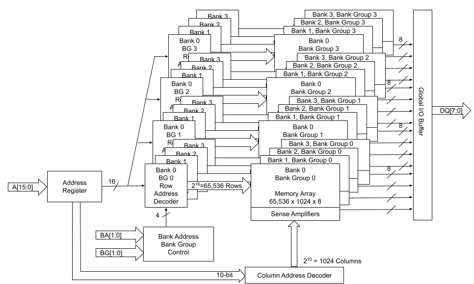
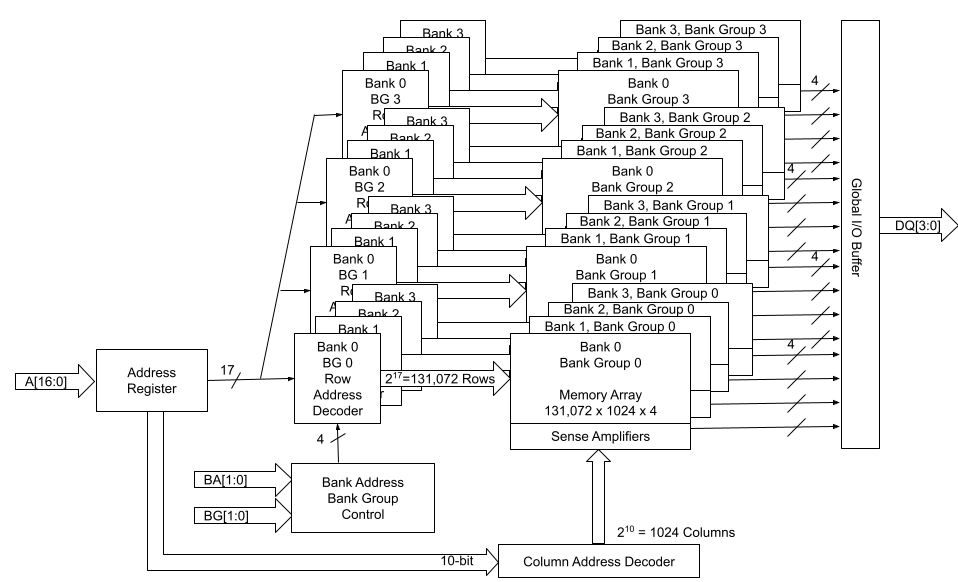
Let’s look at the following two high-level block diagrams of 1Gbx8 and 2Gbx4 memory chips. The total memory capacity for both of them is 8Gb. Figure 2 describes the 1Gb x8 configuration, and Figure 3 describes the 2Gbx4 configuration. With DDR4, both x4 and x8 devices have 4 groups of 4 banks. x16 devices have 2 groups of 4 banks.
We can think of each memory chip as a library. Within that library, there are four bank groups, which are the four floors of the library. On each floor, there are four shelves, each shelf is similar to one of the banks. And we can locate each one of the memory cells by its row and column addresses, just like the library book call numbers. Within each bank, the row address MUX activates a line in the memory array through the Row address latch and decoder, based on the given row address. This line is also called the word line. When a word line is activated, the data on the word line is loaded on to the sense amplifiers. Subsequently, the column decoder accesses the data on the sense amplifier based on the given column address.
Figure 2: 1Gbx8 block diagram
The capacity, or density of a memory chip is calculated as:
Memory Depth = Number of Rows * Number of Columns * Number of Banks
Total Memory Capacity = Memory Depth * Memory Width
In the example of a 1Gbx8 device as shown in Figure 2 above:
Figure 3 describes the function block diagram of a 2 Gb x 4 device.
Figure 3: 2Gbx4 Block Diagram
Number of Row Address Bits = 17
Total Number of Rows = 2 ^ 17 = 131072
Number of Column Address Bits = 10
Total Number of Columns = 2 ^ 10 = 1024
And the calculation goes:
Memory Depth = 131072 * 1024 * 16 = 2Gb
Total Memory Capacity = 2Gb* 4 = 8Gb
Memory module capacity
Memory rank and memory width determine how many memory devices are needed on each memory module.
A 64-bit DDR4 module with ECC support has a total of 72 bits for the data bus. Of the 72 bits, 8 bits are used for ECC. It would require a total of 18 x4 memory devices for a single rank module. Each memory device would supply 4 bits, and the total number of bits with 18 devices is 72 bits. For a dual rank module, we would need to double the amount of memory devices to 36.
If each x4 memory device has a memory capacity of 8Gb, a single rank module with 16 + 2 (ECC) devices would have 16GB module capacity.
8Gb * 16 = 128Gb = 16GB
And a dual rank ECC module with 36 8Gb (2Gb x 4) devices would have 32GB module capacity.
8Gb * 32 = 256Gb = 32GB
If the memory devices are x8, a 64-bit DDR4 module with ECC support would require a total of 9 x8 memory devices for a single rank module, and 18 x8 memory devices for a dual rank memory module. If each of these x8 memory devices has a memory capacity of 8Gb, a single rank module would have 8GB module capacity.
8Gb * 8 = 64Gb = 8GB
A dual rank ECC module with 18 8Gb (1Gb x 8) devices would have 16GB module capacity.
8Gb * 16 = 128Gb = 16GB
Notice that within the same memory device technology, for example 8Gb in our example, higher memory module capacity is achieved through using x4 device width, or dual-rank, or even quad-rank.
ACTIVATE timing and DRAM page sizes
Memory device width, whether it is x4, x8 or x16, also has an effect on memory timing parameters such as tFAW.
tFAW refers to Four Active Window time. It specifies a timing window within which four ACTIVATE commands can be issued. An ACTIVATE command is issued to open a row within a bank. In the block diagrams above we can see that each bank has its own set of sense amplifiers, thus one row can remain active per bank. A memory controller can issue four back-to-back ACTIVATE commands, but once the fourth ACTIVATE is done, the fifth ACTIVATE cannot be issued until the tFAW window expires.
The table below lists out the tFAW window lengths assigned to various DDR4 speeds and page sizes. Notice that under the same DDR4 speed, the bigger the page size, the longer the tFAW window is. For example, DDR4-1600 has a tFAW window of 20ns with 1/2KB page size. This means that within a bank, once a command to open a first row is issued, the controller must wait for 20ns, or 16 clock cycles (CK) before a command to open a fifth row can be issued.
The JEDEC memory standard specification for DDR4 tFAW timing varies by page sizes: 1/2KB, 1KB and 2KB.
Symbol
DDR4-1600
DDR4-1866
DDR4-2133
DDR4-2400
Four ACTIVATE windows for 1/2KB page size (minimum)
tFAW (1/2KB)
greater of 16CK or 20ns
greater of 16CK or 17ns
greater of 16CK or 15ns
greater of 16CK or 13ns
Four ACTIVATE windows for 1KB page size (minimum)
tFAW (1KB)
greater of 20CK or 25ns
greater of 20CK or 23ns
greater of 20CK or 21ns
greater of 20CK or 21ns
Four ACTIVATE windows for 2KB page size (minimum)
tFAW (2KB)
greater of 28CK or 35ns
greater of 28CK or 30ns
greater of 28CK or 30ns
greater of 28CK or 30ns
What is the relationship between page sizes and memory device width? Since we briefly compared two 8Gb memory devices earlier, it makes sense to take another look at those two in terms of page sizes.
Page size is the number of bits loaded into the sense amplifiers when a row is activated. Therefore page size is directly related to the number of bits per row, or number of columns per row.
Page Size = Number of Columns * Memory Device Width = 1024 * Memory Device Width
The table below shows the page sizes for each device width:
Device Width
Page Size (Kb)
Page Size (KB)
x4
4 Kb
1/2 KB
x8
8 Kb
1 KB
x16
16 Kb
2 KB
Among the three device widths, x4 devices have the shortest tFAW timing limit, and x16 devices have the longest tFAW timing limit. The difference in tFAW specification has a negative timing performance impact on devices with higher device width.
An experiment with 2Rx4 and 2Rx8 DDR4 modules
To quantify the impact on memory performance from different memory device widths, an experiment has been conducted on our Gen11 servers with AMD EPYC 7713 Rome CPU. The Rome CPU has 64 cores, supports 8 memory channels.
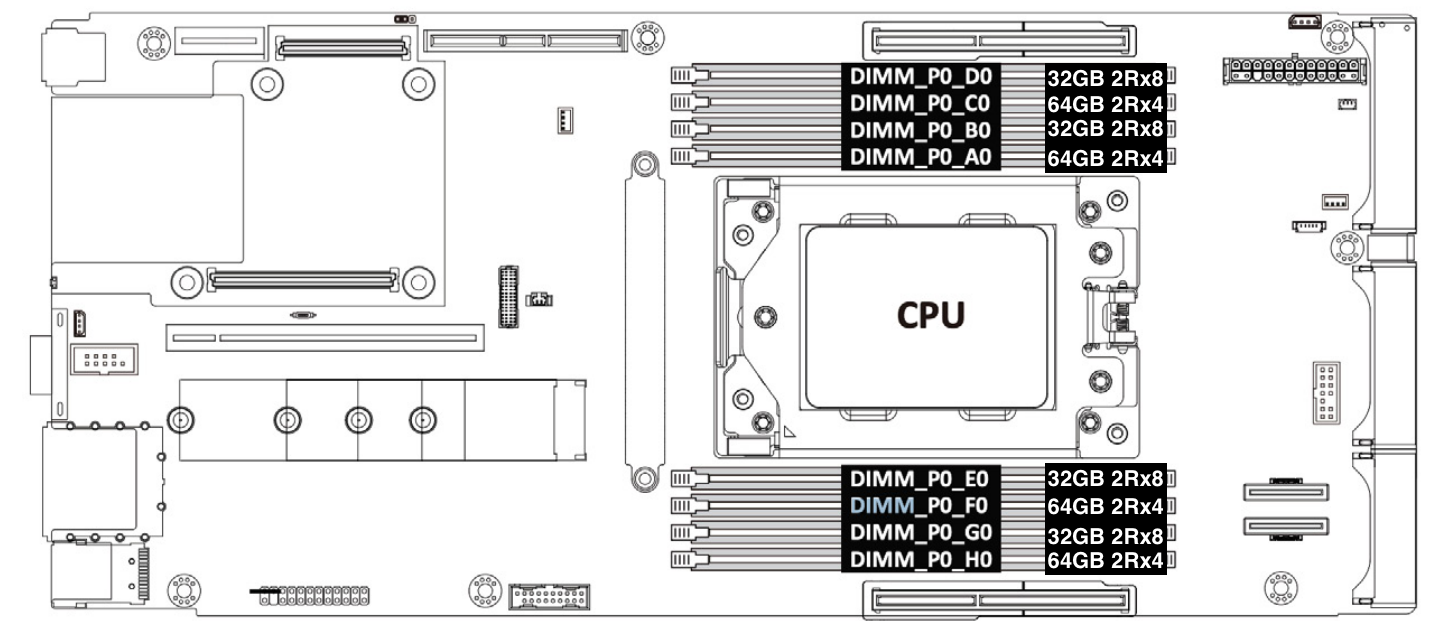
Our production Gen11 servers are configured with 1 DIMM populated in each memory channel. In order to achieve 6GB/core memory per core ratio, the total memory for the Gen11 system is 64 core * 6 GB/core = 384 GB. This is achieved by installing four pieces of 32GB 2Rx8 and four pieces of 64GB 2Rx4 memory modules.
Figure 5: Gen11 server memory configuration
To compare the bandwidth performance difference between 2Rx4 and 2Rx8 DDR4 modules, two test cases are needed. One with all 2Rx4 DDR4 modules, and another one with 2Rx8 DDR4 modules. Each test case populates eight pieces of 32GB 32Mbps DDR4 RDIMM memories in each memory channel (1DPC). As shown in the table below, the difference between the set up of the two test cases is: case A tests 2Rx4 memory modules, and case B tests 2Rx8 memory modules.
Test case
Number of DIMMs
Memory vendor
Part number
Memory size
Memory speed
Memory organization
A
8
Samsung
M393A4G43BB4-CWE
32GB
3200 MT/s
2Rx8
B
8
Samsung
M393A4K40EB3-CWECQ
32GB
3200 MT/s
2Rx4
Memory Latency Checker results
Memory Latency Checker is an Intel developed synthetic benchmarking tool. It measures memory latency and bandwidth, and how they vary with workloads of different read/write ratios, as well as stream triad. Stream triad is a memory benchmark workload that contains three operations: it first multiples a large 1D array with a scalar, then adds it to a second array, and assigns it to a third array.
2Rx8 32GB bandwidth (MB/s)
2Rx4 32GB bandwidth (MB/s)
Percentage difference
All reads
173,287
173,650
0.21%
3:1 reads-writes
154,593
156,343
1.13%
2:1 reads-writes
151,660
155,289
2.39%
1:1 reads-writes
146,895
151,199
2.93%
Stream-triad like
156,273
158,710
1.56%
The bandwidth performance difference in the All reads test case is not very significant, only 0.21%.
As the amount of writes increase, from 25% (3:1 reads-writes) to 50% (1:1 reads-writes), the bandwidth performance differences between test case A and test case B increase from 1.13% to 2.93%.
LMBench Results
LMBench is another synthetic benchmarking tool often used to study bandwidth performances of memory. Our LMBench bw_mem tests results are comparable to the results obtained from the MLC benchmark test.
2Rx8 32GB bandwidth (MB/s)
2Rx4 32GB bandwidth (MB/s)
Percentage difference
Read
170,285
173,897
2.12%
Write
73,179
76,019
3.88%
Read then write
72,804
74,926
2.91%
Copy
50,332
51,776
2.87%
The biggest bandwidth performance difference is with Write workload. The 2Rx4 test case has 3.88% higher write bandwidth than the 2Rx8 test case.
Summary
Memory organization and memory width has a slight effect on memory bandwidth performance. The difference is most obvious in write-heavy workloads than read-heavy workloads. But even in write-heavy workloads, the difference is less than 4% according to our benchmark tests.
Memory modules with x4 width require twice the number of memory devices on the memory module, as compared to memory modules with x8 width of the same capacity. More memory devices would consume more power. According to Micron’s measurement data, 2Rx8 32GB memory modules using 16Gb devices consume 31% less power than 2Rx4 32GB memory modules using 8Gb devices. The substantial power saving of using x8 memory modules may outweigh the slight bandwidth performance impact.
Our Gen11 servers are configured with a mix of 2Rx4 and 2Rx8 DDR4 modules. For our future generations, we may consider using 2Rx8 memory where possible, in order to reduce overall system power consumption, with minimal impact to bandwidth performance.
EFF has a good explainer on the problems with the new UN Cybercrime Treaty, currently being negotiated in Vienna.
The draft treaty has the potential to rewrite criminal laws around the world, possibly adding over 30 criminal offenses and new expansive police powers for both domestic and international criminal investigations.
The 2023 Linux Plumbers Conference (November 13-15, Richmond VA, USA) has
put out its calls for proposals for the
refereed track (due August 6) and the
microconference track (June 1). Proposals are also being accepted
for the kernel-summit track.
For developers seeking to create applications with terminal user
interfaces (TUIs), options have been relatively limited compared to the
vast number of graphical user interface (GUI) frameworks available. As a
result, many command-line applications reinvent the same user interface
elements. Textual aims to
remedy this: it’s a rapid-application-development framework for
Python TUI applications. Offering cross-platform support, Textual
incorporates layouts, CSS-like styles, and an expanding collection of
widgets.
Richard Brown has posted an
update on the status of the SUSE Adaptable Linux Platform (ALP) project
and what it means for the openSUSE distribution.
The ALP concept should be flexible enough that these openSUSE
Products will be able to leverage all the stuff SUSE is doing for
SUSE’s ALP Products, but then we (community) can add anything we
want. If we find it is not flexible enough, then we (SUSE) will
work to adapt it to make it possible for the community to build
what it wants.
So, if we the community want to build something like old Leap, that
should be totally technically feasible.
The collective thoughts of the interwebz
Manage Consent
To provide the best experiences, we use technologies like cookies to store and/or access device information. Consenting to these technologies will allow us to process data such as browsing behavior or unique IDs on this site. Not consenting or withdrawing consent, may adversely affect certain features and functions.
Functional
Always active
The technical storage or access is strictly necessary for the legitimate purpose of enabling the use of a specific service explicitly requested by the subscriber or user, or for the sole purpose of carrying out the transmission of a communication over an electronic communications network.
Preferences
The technical storage or access is necessary for the legitimate purpose of storing preferences that are not requested by the subscriber or user.
Statistics
The technical storage or access that is used exclusively for statistical purposes.The technical storage or access that is used exclusively for anonymous statistical purposes. Without a subpoena, voluntary compliance on the part of your Internet Service Provider, or additional records from a third party, information stored or retrieved for this purpose alone cannot usually be used to identify you.
Marketing
The technical storage or access is required to create user profiles to send advertising, or to track the user on a website or across several websites for similar marketing purposes.


 Moira Lennox is a Senior Data Strategy Technical Specialist for AWS with 27 years’ experience helping companies innovate and modernize their data strategies to achieve new heights and allow for strategic decision-making. She has experience working in large enterprises and technology providers, in both business and technical roles across multiple industries, including health care live sciences, financial services, communications, digital entertainment, energy, and manufacturing.
 Joel Farvault is Principal Specialist SA Analytics for AWS with 25 years’ experience working on enterprise architecture, data strategy, and analytics, mainly in the financial services industry. Joel has led data transformation projects on fraud analytics, claims automation, and data governance.
 Mike Havey is a Solutions Architect for AWS with over 25 years of experience building enterprise applications. Mike is the author of two books and numerous articles. His


 Vinay Kumar Khambhampati is a Lead Consultant with the AWS ProServe Team, helping customers with cloud adoption. He is passionate about big data and data analytics.
 Sandeep Singh is a Lead Consultant at AWS ProServe, focused on analytics, data lake architecture, and implementation. He helps enterprise customers migrate and modernize their data lake and data warehouse using AWS services.
 Amol Guldagad is a Data Analytics Consultant based in India. He has worked with customers in different industries like banking and financial services, healthcare, power and utilities, manufacturing, and retail, helping them solve complex challenges with large-scale data platforms. At AWS ProServe, he helps customers accelerate their journey to the cloud and innovate using AWS analytics services.