Summer has drawn to a close here in Utrecht, where I live in the Netherlands. In two weeks, I’ll be attending AWS Community Day 2025, hosted at the Kinepolis Jaarbeurs Utrecht on September 24. The single-day event will bring together over 500 cloud practitioners from across the Netherlands, featuring 25 breakout sessions across five technical tracks. The day will begin with virtual keynotes at 9:00 AM, followed by parallel breakout sessions focused on practical implementations of serverless architectures and container optimization strategies, providing valuable insights regardless of experience level.
Last year’s AWS Community Day Netherlands 2024 brought together a diverse group of cloud practitioners, speakers, and AWS enthusiasts who contributed to making the community-led conference a valuable knowledge-sharing platform. If you’re planning to attend, feel free to find me there to discuss AWS services or share your cloud implementation experiences!
Let’s look at last week’s new announcements.
Last week’s launches
AWS Transform assessments now includes detached storage analysis – AWS Transform has expanded its assessment capabilities to analyze on-premises detached storage infrastructure, helping customers determine migration total cost of ownership (TCO). The assessment now evaluates Storage Area Network (SAN), Network Attached Storage (NAS), file servers, object storage, and virtual environments, providing migration recommendations to appropriate AWS services including Amazon S3, Amazon EBS, and Amazon FSx. The tool delivers a comprehensive TCO comparison between current and AWS environments, along with performance and cost optimization recommendations. With storage accounting for up to 45% of total migration opportunities, this enhancement helps customers visualize various AWS migration options. AWS Transform assessment is available in US East (N. Virginia) and Europe (Frankfurt) Regions.
Amazon Bedrock introduces Global Cross-Region inference for Anthropic Claude Sonnet 4 – Anthropic’s Claude Sonnet 4 model in Amazon Bedrock now supports Global cross-Region inference, allowing inference requests to route to any supported commercial AWS Region for processing. This enhancement optimizes available resources and enables higher model throughput by distributing traffic across multiple Regions. Previously, you could select cross-Region inference profiles tied to specific geographies (US, EU, or APAC). The new Global cross-Region inference profile provides additional flexibility for generative AI use cases that don’t require geography-specific processing, helping manage unplanned traffic bursts and increase model throughput. For detailed implementation guidance, visit the Amazon Bedrock documentation.
Amazon Neptune Database adds Public Endpoints support – Amazon Neptune now supports Public Endpoints, enabling direct connections to Neptune databases from outside the VPC without complex networking configurations. This feature helps developers securely access their graph databases from development desktops without requiring VPN connections or bastion hosts, while maintaining security through IAM authentication, VPC security groups, and encryption in transit. Public Endpoints can be enabled for Neptune clusters running engine version 1.4.6 or above through the AWS Management Console, AWS CLI, or AWS SDK. The feature is available at no additional cost beyond standard Neptune pricing in all AWS Regions where Neptune Database is offered. Implementation details are available in the Amazon Neptune documentation.
ECS Exec now available in AWS Management Console – Amazon ECS now supports ECS Exec directly in the AWS Management Console, enabling secure, interactive shell access to running containers without requiring inbound ports or SSH key management. Previously available only through API, CLI, or SDKs, this feature streamlines troubleshooting by allowing container access directly from the console interface. You can enable ECS Exec when creating or updating services and standalone tasks, then connect to containers by selecting “Connect” on the task details page, which opens an interactive session through CloudShell. The console also displays the underlying AWS CLI command for use in local terminals. This feature is available in all AWS commercial Regions and documented in the ECS developer guide.
Organizational Notification Configurations for AWS User Notifications now generally available – AWS User Notifications now supports Organizational Notification Configurations, helping AWS Organizations users centrally configure and view notifications across their organization. Management accounts or delegated administrators can configure notifications for specific organizational units or all accounts in an organization. The service supports configuring notifications for any supported Amazon EventBridge event, such as console sign-ins without MFA, with notifications appearing in the admin’s Console Notifications Center and AWS Console Mobile Application. User Notifications supports up to five delegated administrators and is available in all AWS Regions where AWS User Notifications is offered. For implementation details, visit the AWS User Notifications user guide.
Upcoming AWS events Check your calendar and sign up for upcoming AWS events.
AWS Summits – Join free online and in-person events that bring the cloud computing community together to connect, collaborate, and learn about AWS. Register in your nearest city: Zurich (September 11), Los Angeles (September 17), and Bogotá (October 9).
AWS re:Invent 2025 – Join us in Las Vegas between December 1–5 as cloud pioneers gather from across the globe for the latest AWS innovations, peer-to-peer learning, expert-led discussions, and invaluable networking opportunities. Don’t forget to explore the event catalog.
AWS Community Days – Join community-led conferences that feature technical discussions, workshops, and hands-on labs led by expert AWS users and industry leaders from around the world: Baltic (September 10), Aotearoa (September 18), South Africa (September 20), Bolivia (September 20), Portugal (September 27).
AWS Summit season starts this week! These free events are now rolling out worldwide, bringing our cloud computing community together to connect, collaborate, and learn. Whether you prefer joining us online or in-person, these gatherings offer valuable opportunities to expand your AWS knowledge. I will be attending the Summit in Paris this week, the biggest cloud conference in France, and the London Summit at the end of the month. We will have a small podcast recording studio where I will interview French and British customers to produce new episodes for the AWS Developers Podcast and le podcast AWS en .
Register today!
But for now, let’s look at last week’s new announcements.
Last week’s launches At KubeCon London, we introduced the EKS Community Add-Ons Catalog, making it simpler for Kubernetes users to enhance their Amazon EKS clusters with powerful open-source tools. This catalog streamlines the installation of essential add-ons like metrics-server, kube-state-metrics, prometheus-node-exporter, cert-manager, and external-dns. By integrating these community-driven add-ons directly into the EKS console and AWS command line interface (AWS CLI), customers can reduce operational complexity and accelerate deployment while maintaining flexibility and security. This launch reflects AWS’s commitment to the Kubernetes community, providing seamless access to trusted open-source solutions without the overhead of manual installation and maintenance.
Amazon Q Developer now integrates with Amazon OpenSearch Service to enhance operational analytics by enabling natural language exploration and AI-assisted data visualization. This integration simplifies the process of querying and visualizing operational data, reducing the learning curve associated with traditional query languages and tools. During incident responses, Amazon Q Developer offers contextual summaries and insights directly within the alerts interface, facilitating quicker analysis and resolution. This advancement allows engineers to focus more on innovation by streamlining troubleshooting processes and improving monitoring infrastructure.
Amazon SES has introduced support for email attachments in its v2 APIs, enabling users to include files like PDFs and images directly in their emails without manually constructing MIME messages. This enhancement simplifies the process of sending rich email content and reduces implementation complexity. Amazon Simple Email Service (Amazon SES) supports attachments in all AWS Regions where the service is available.
Other AWS events Check your calendar and sign up for upcoming AWS events.
AWS GenAI Lofts are collaborative spaces and immersive experiences that showcase AWS expertise in cloud computing and AI. They provide startups and developers with hands-on access to AI products and services, exclusive sessions with industry leaders, and valuable networking opportunities with investors and peers. Find a GenAI Loft location near you and don’t forget to register.
(This survey is hosted by an external company. AWS handles your information as described in the AWS Privacy Notice. AWS will own the data gathered via this survey and will not share the information collected with survey respondents.)
One-time and complex queries are two common scenarios in enterprise data analytics. One-time queries are flexible and suitable for instant analysis and exploratory research. Complex queries, on the other hand, refer to large-scale data processing and in-depth analysis based on petabyte-level data warehouses in massive data scenarios. These complex queries typically involve data sources from multiple business systems, requiring multilevel nested SQL or associations with numerous tables for highly sophisticated analytical tasks.
However, combining the data lineage of these two query types presents several challenges:
Diversity of data sources
Varying query complexity
Inconsistent granularity in lineage tracking
Different real-time requirements
Difficulties in cross-system integration
Moreover, maintaining the accuracy and completeness of lineage information while providing system performance and scalability are crucial considerations. Addressing these challenges requires a carefully designed architecture and advanced technical solutions.
Amazon Athena offers serverless, flexible SQL analytics for one-time queries, enabling direct querying of Amazon Simple Storage Service (Amazon S3) data for rapid, cost-effective instant analysis. Amazon Redshift, optimized for complex queries, provides high-performance columnar storage and massively parallel processing (MPP) architecture, supporting large-scale data processing and advanced SQL capabilities. Amazon Neptune, as a graph database, is ideal for data lineage analysis, offering efficient relationship traversal and complex graph algorithms to handle large-scale, intricate data lineage relationships. The combination of these three services provides a powerful, comprehensive solution for end-to-end data lineage analysis.
In the context of comprehensive data governance, Amazon DataZone offers organization-wide data lineage visualization using Amazon Web Services (AWS) services, while dbt provides project-level lineage through model analysis and supports cross-project integration between data lakes and warehouses.
In this post, we use dbt for data modeling on both Amazon Athena and Amazon Redshift. dbt on Athena supports real-time queries, while dbt on Amazon Redshift handles complex queries, unifying the development language and significantly reducing the technical learning curve. Using a single dbt modeling language not only simplifies the development process but also automatically generates consistent data lineage information. This approach offers robust adaptability, easily accommodating changes in data structures.
By integrating Amazon Neptune graph database to store and analyze complex lineage relationships, combined with AWS Step Functions and AWS Lambda functions, we achieve a fully automated data lineage generation process. This combination promotes consistency and completeness of lineage data while enhancing the efficiency and scalability of the entire process. The result is a powerful and flexible solution for end-to-end data lineage analysis.
Architecture overview
The experiment’s context involves a customer already using Amazon Athena for one-time queries. To better accommodate massive data processing and complex query scenarios, they aim to adopt a unified data modeling language across different data platforms. This led to the implementation of both Athena on dbt and Amazon Redshift on dbt architectures.
AWS Glue crawler crawls data lake information from Amazon S3, generating a Data Catalog to support dbt on Amazon Athena data modeling. For complex query scenarios, AWS Glue performs extract, transform, and load (ETL) processing, loading data into the petabyte-scale data warehouse, Amazon Redshift. Here, data modeling uses dbt on Amazon Redshift.
Lineage data original files from both parts are loaded into an S3 bucket, providing data support for end-to-end data lineage analysis.
The following image is the architecture diagram for the solution.
This experiment uses the following data dictionary:
Source table
Tool
Target table
imdb.name_basics
DBT/Athena
stg_imdb__name_basics
imdb.title_akas
DBT/Athena
stg_imdb__title_akas
imdb.title_basics
DBT/Athena
stg_imdb__title_basics
imdb.title_crew
DBT/Athena
stg_imdb__title_crews
imdb.title_episode
DBT/Athena
stg_imdb__title_episodes
imdb.title_principals
DBT/Athena
stg_imdb__title_principals
imdb.title_ratings
DBT/Athena
stg_imdb__title_ratings
stg_imdb__name_basics
DBT/Redshift
new_stg_imdb__name_basics
stg_imdb__title_akas
DBT/Redshift
new_stg_imdb__title_akas
stg_imdb__title_basics
DBT/Redshift
new_stg_imdb__title_basics
stg_imdb__title_crews
DBT/Redshift
new_stg_imdb__title_crews
stg_imdb__title_episodes
DBT/Redshift
new_stg_imdb__title_episodes
stg_imdb__title_principals
DBT/Redshift
new_stg_imdb__title_principals
stg_imdb__title_ratings
DBT/Redshift
new_stg_imdb__title_ratings
new_stg_imdb__name_basics
DBT/Redshift
int_primary_profession_flattened_from_name_basics
new_stg_imdb__name_basics
DBT/Redshift
int_known_for_titles_flattened_from_name_basics
new_stg_imdb__name_basics
DBT/Redshift
names
new_stg_imdb__title_akas
DBT/Redshift
titles
new_stg_imdb__title_basics
DBT/Redshift
int_genres_flattened_from_title_basics
new_stg_imdb__title_basics
DBT/Redshift
titles
new_stg_imdb__title_crews
DBT/Redshift
int_directors_flattened_from_title_crews
new_stg_imdb__title_crews
DBT/Redshift
int_writers_flattened_from_title_crews
new_stg_imdb__title_episodes
DBT/Redshift
titles
new_stg_imdb__title_principals
DBT/Redshift
titles
new_stg_imdb__title_ratings
DBT/Redshift
titles
int_known_for_titles_flattened_from_name_basics
DBT/Redshift
titles
int_primary_profession_flattened_from_name_basics
DBT/Redshift
int_directors_flattened_from_title_crews
DBT/Redshift
names
int_genres_flattened_from_title_basics
DBT/Redshift
genre_titles
int_writers_flattened_from_title_crews
DBT/Redshift
names
genre_titles
DBT/Redshift
names
DBT/Redshift
titles
DBT/Redshift
The lineage data generated by dbt on Athena includes partial lineage diagrams, as exemplified in the following images. The first image shows the lineage of name_basics in dbt on Athena. The second image shows the lineage of title_crew in dbt on Athena.
The lineage data generated by dbt on Amazon Redshift includes partial lineage diagrams, as illustrated in the following image.
Referring to the data dictionary and screenshots, it’s evident that the complete data lineage information is highly dispersed, spread across 29 lineage diagrams. Understanding the end-to-end comprehensive view requires significant time. In real-world environments, the situation is often more complex, with complete data lineage potentially distributed across hundreds of files. Consequently, integrating a complete end-to-end data lineage diagram becomes crucial and challenging.
This experiment will provide a detailed introduction to processing and merging data lineage files stored in Amazon S3, as illustrated in the following diagram.
Prerequisites
To perform the solution, you need to have the following prerequisites in place:
The Lambda function for preprocessing lineage files must have permissions to access Amazon S3 and Amazon Redshift.
The Lambda function for constructing the directed acyclic graph (DAG) must have permissions to access Amazon S3 and Amazon Neptune.
Solution walkthrough
To perform the solution, follow the steps in the next sections.
Preprocess raw lineage data for DAG generation using Lambda functions
Use Lambda to preprocess the raw lineage data generated by dbt, converting it into key-value pair JSON files that are easily understood by Neptune: athena_dbt_lineage_map.json and redshift_dbt_lineage_map.json.
To create a new Lambda function in the Lambda console, enter a Function name, select the Runtime (Python in this example), configure the Architecture and Execution role, then click the “Create function” button.
Open the created Lambda function and on the Configuration tab, in the navigation pane, select Environment variables and choose your configurations. Using Athena on dbt processing as an example, configure the environment variables as follows (the process for Amazon Redshift on dbt is similar):
INPUT_BUCKET: data-lineage-analysis-24-09-22 (replace with the S3 bucket path storing the original Athena on dbt lineage files)
INPUT_KEY: athena_manifest.json (the original Athena on dbt lineage file)
OUTPUT_BUCKET: data-lineage-analysis-24-09-22 (replace with the S3 bucket path for storing the preprocessed output of Athena on dbt lineage files)
OUTPUT_KEY: athena_dbt_lineage_map.json (the output file after preprocessing the original Athena on dbt lineage file)
On the Code tab, in the lambda_function.py file, enter the preprocessing code for the raw lineage data. Here’s a code reference using Athena on dbt processing as an example (the process for Amazon Redshift on dbt is similar). The preprocessing code for Athena on dbt’s original lineage file is as follows:
import json
import boto3
import os

def lambda_handler(event, context):
    # Set up S3 client
    s3 = boto3.client('s3')

    # Get input and output paths from environment variables
    input_bucket = os.environ['INPUT_BUCKET']
    input_key = os.environ['INPUT_KEY']
    output_bucket = os.environ['OUTPUT_BUCKET']
    output_key = os.environ['OUTPUT_KEY']

    # Define helper function
    def dbt_nodename_format(node_name):
        return node_name.split(".")[-1]

    # Read input JSON file from S3
    response = s3.get_object(Bucket=input_bucket, Key=input_key)
    file_content = response['Body'].read().decode('utf-8')
    data = json.loads(file_content)
    lineage_map = data["child_map"]
    node_dict = {}
    dbt_lineage_map = {}

    # Process data
    for item in lineage_map:
        lineage_map[item] = [dbt_nodename_format(child) for child in lineage_map[item]]
        node_dict[item] = dbt_nodename_format(item)

    # Update key names
    lineage_map = {node_dict[old]: value for old, value in lineage_map.items()}
    dbt_lineage_map["lineage_map"] = lineage_map

    # Convert result to JSON string
    result_json = json.dumps(dbt_lineage_map)

    # Write JSON string to S3
    s3.put_object(Body=result_json, Bucket=output_bucket, Key=output_key)
    print(f"Data written to s3://{output_bucket}/{output_key}")

    return {
        'statusCode': 200,
        'body': json.dumps('Athena data lineage processing completed successfully')
    }
Merge preprocessed lineage data and write to Neptune using Lambda functions
Before processing data with the Lambda function, create a Lambda layer by uploading the required Gremlin plugin. For detailed steps on creating and configuring Lambda Layers, see the AWS Lambda Layers documentation.
Because connecting Lambda to Neptune for constructing a DAG requires the Gremlin plugin, it needs to be uploaded before using Lambda. The Gremlin package can be obtained from the Data Lineage Graph Construction GitHub repository.
Create a new Lambda function. Choose the function to configure. To the recently created layer, at the bottom of the page, choose Add a layer.
Create another Lambda layer for the requests library, similar to how you created the layer for the Gremlin plugin. This library will be used for HTTP client functionality in the Lambda function.
Choose the recently created Lambda function to configure. Connect to Neptune through Lambda to merge the two datasets and construct a DAG. On the Code tab, the reference code to execute is as follows:
import json
import boto3
import os
import requests
from botocore.auth import SigV4Auth
from botocore.awsrequest import AWSRequest
from botocore.credentials import get_credentials
from botocore.session import Session
from concurrent.futures import ThreadPoolExecutor, as_completed

def read_s3_file(s3_client, bucket, key):
    try:
        response = s3_client.get_object(Bucket=bucket, Key=key)
        data = json.loads(response['Body'].read().decode('utf-8'))
        return data.get("lineage_map", {})
    except Exception as e:
        print(f"Error reading S3 file {bucket}/{key}: {str(e)}")
        raise

def merge_data(athena_data, redshift_data):
    return {**athena_data, **redshift_data}

def sign_request(request):
    credentials = get_credentials(Session())
    auth = SigV4Auth(credentials, 'neptune-db', os.environ['AWS_REGION'])
    auth.add_auth(request)
    return dict(request.headers)

def send_request(url, headers, data):
    try:
        response = requests.post(url, headers=headers, data=data, timeout=30)
        response.raise_for_status()
        return response.text
    except requests.exceptions.RequestException as e:
        print(f"Request Error: {str(e)}")
        if hasattr(e.response, 'text'):
            print(f"Response content: {e.response.text}")
        raise

def write_to_neptune(data):
    endpoint = 'https://your neptune endpoint name:8182/gremlin'
    # replace with your neptune endpoint name

    # Clear Neptune database
    clear_query = "g.V().drop()"
    request = AWSRequest(method='POST', url=endpoint, data=json.dumps({'gremlin': clear_query}))
    signed_headers = sign_request(request)
    response = send_request(endpoint, signed_headers, json.dumps({'gremlin': clear_query}))
    print(f"Clear database response: {response}")

    # Verify if the database is empty
    verify_query = "g.V().count()"
    request = AWSRequest(method='POST', url=endpoint, data=json.dumps({'gremlin': verify_query}))
    signed_headers = sign_request(request)
    response = send_request(endpoint, signed_headers, json.dumps({'gremlin': verify_query}))
    print(f"Vertex count after clearing: {response}")

    def process_node(node, children):
        # Add node
        query = f"g.V().has('lineage_node', 'node_name', '{node}').fold().coalesce(unfold(), addV('lineage_node').property('node_name', '{node}'))"
        request = AWSRequest(method='POST', url=endpoint, data=json.dumps({'gremlin': query}))
        signed_headers = sign_request(request)
        response = send_request(endpoint, signed_headers, json.dumps({'gremlin': query}))
        print(f"Add node response for {node}: {response}")

        for child_node in children:
            # Add child node
            query = f"g.V().has('lineage_node', 'node_name', '{child_node}').fold().coalesce(unfold(), addV('lineage_node').property('node_name', '{child_node}'))"
            request = AWSRequest(method='POST', url=endpoint, data=json.dumps({'gremlin': query}))
            signed_headers = sign_request(request)
            response = send_request(endpoint, signed_headers, json.dumps({'gremlin': query}))
            print(f"Add child node response for {child_node}: {response}")

            # Add edge
            query = f"g.V().has('lineage_node', 'node_name', '{node}').as('a').V().has('lineage_node', 'node_name', '{child_node}').coalesce(inE('lineage_edge').where(outV().as('a')), addE('lineage_edge').from('a').property('edge_name', ' '))"
            request = AWSRequest(method='POST', url=endpoint, data=json.dumps({'gremlin': query}))
            signed_headers = sign_request(request)
            response = send_request(endpoint, signed_headers, json.dumps({'gremlin': query}))
            print(f"Add edge response for {node} -> {child_node}: {response}")

    with ThreadPoolExecutor(max_workers=10) as executor:
        futures = [executor.submit(process_node, node, children) for node, children in data.items()]
        for future in as_completed(futures):
            try:
                future.result()
            except Exception as e:
                print(f"Error in processing node: {str(e)}")

def lambda_handler(event, context):
    # Initialize S3 client
    s3_client = boto3.client('s3')

    # S3 bucket and file paths
    bucket_name = 'data-lineage-analysis' # Replace with your S3 bucket name
    athena_key = 'athena_dbt_lineage_map.json' # Replace with your athena lineage key value output json name
    redshift_key = 'redshift_dbt_lineage_map.json' # Replace with your redshift lineage key value output json name

    try:
        # Read Athena lineage data
        athena_data = read_s3_file(s3_client, bucket_name, athena_key)
        print(f"Athena data size: {len(athena_data)}")

        # Read Redshift lineage data
        redshift_data = read_s3_file(s3_client, bucket_name, redshift_key)
        print(f"Redshift data size: {len(redshift_data)}")

        # Merge data
        combined_data = merge_data(athena_data, redshift_data)
        print(f"Combined data size: {len(combined_data)}")

        # Write to Neptune (including clearing the database)
        write_to_neptune(combined_data)

        return {
            'statusCode': 200,
            'body': json.dumps('Data successfully written to Neptune')
        }
    except Exception as e:
        print(f"Error in lambda_handler: {str(e)}")
        return {
            'statusCode': 500,
            'body': json.dumps(f'Error: {str(e)}')
        }
Create Step Functions workflow
On the Step Functions console, choose State machines, and then choose Create state machine. On the Choose a template page, select Blank template.
In the Blank template, choose Code to define your state machine. Use the following example code:
{
  "Comment": "Daily Data Lineage Processing Workflow",
  "StartAt": "Parallel Processing",
  "States": {
    "Parallel Processing": {
      "Type": "Parallel",
      "Branches": [
        {
          "StartAt": "Process Athena Data",
          "States": {
            "Process Athena Data": {
              "Type": "Task",
              "Resource": "arn:aws:states:::lambda:invoke",
              "Parameters": {
                "FunctionName": "athena-data-lineange-process-Lambda", ##Replace with your Athena data lineage process Lambda function name
                "Payload": {
                  "input.$": "$"
                }
              },
              "End": true
            }
          }
        },
        {
          "StartAt": "Process Redshift Data",
          "States": {
            "Process Redshift Data": {
              "Type": "Task",
              "Resource": "arn:aws:states:::lambda:invoke",
              "Parameters": {
                "FunctionName": "redshift-data-lineange-process-Lambda", ##Replace with your Redshift data lineage process Lambda function name
                "Payload": {
                  "input.$": "$"
                }
              },
              "End": true
            }
          }
        }
      ],
      "Next": "Load Data to Neptune"
    },
    "Load Data to Neptune": {
      "Type": "Task",
      "Resource": "arn:aws:states:::lambda:invoke",
      "Parameters": {
        "FunctionName": "data-lineage-analysis-lambda" ##Replace with your Lambda function Name
      },
      "End": true
    }
  }
}
After completing the configuration, choose the Design tab to view the workflow shown in the following diagram.
Create scheduling rules with Amazon EventBridge
Configure Amazon EventBridge to generate lineage data daily during off-peak business hours. To do this:
Create a new rule in the EventBridge console with a descriptive name.
Set the rule type to “Schedule” and configure it to run once daily (using either a fixed rate or the Cron expression “0 0 * * ? *”).
Select the AWS Step Functions state machine as the target and specify the state machine you created earlier.
Query results in Neptune
On the Neptune console, select Notebooks. Open an existing notebook or create a new one.
In the notebook, create a new code cell to perform a query. The following code example shows the query statement and its results:
You can now see the end-to-end data lineage graph information for both dbt on Athena and dbt on Amazon Redshift. The following image shows the merged DAG data lineage graph in Neptune.
You can query the generated data lineage graph for data related to a specific table, such as title_crew.
The sample query statement and its results are shown in the following code example:
In this post, we demonstrated how dbt enables unified data modeling across Amazon Athena and Amazon Redshift, integrating data lineage from both one-time and complex queries. By using Amazon Neptune, this solution provides comprehensive end-to-end lineage analysis. The architecture uses AWS serverless computing and managed services, including Step Functions, Lambda, and EventBridge, providing a highly flexible and scalable design.
This approach significantly lowers the learning curve through a unified data modeling method while enhancing development efficiency. The end-to-end data lineage graph visualization and analysis not only strengthen data governance capabilities but also offer deep insights for decision-making.
The solution’s flexible and scalable architecture effectively optimizes operational costs and improves business responsiveness. This comprehensive approach balances technical innovation, data governance, operational efficiency, and cost-effectiveness, thus supporting long-term business growth with the adaptability to meet evolving enterprise needs.
With OpenLineage-compatible data lineage now generally available in Amazon DataZone, we plan to explore integration possibilities to further enhance the system’s capability to handle complex data lineage analysis scenarios.
If you have any questions, please feel free to leave a comment in the comments section.
About the authors
Nancy Wu is a Solutions Architect at AWS, responsible for cloud computing architecture consulting and design for multinational enterprise customers. Has many years of experience in big data, enterprise digital transformation research and development, consulting, and project management across telecommunications, entertainment, and financial industries.
Xu Feng is a Senior Industry Solution Architect at AWS, responsible for designing, building, and promoting industry solutions for the Media & Entertainment and Advertising sectors, such as intelligent customer service and business intelligence. With 20 years of software industry experience, currently focused on researching and implementing generative AI and AI-powered data solutions.
Xu Da is a Amazon Web Services (AWS) Partner Solutions Architect based out of Shanghai, China. He has more than 25 years of experience in IT industry, software development and solution architecture. He is passionate about collaborative learning, knowledge sharing, and guiding community in their cloud technologies journey.
Externalized authorization for custom applications is a security approach where access control decisions are managed outside of the application logic. Instead of embedding authorization rules within the application’s code, these rules are defined as policies, which are evaluated by a separate system to make an authorization decision. This separation enhances an application’s security posture by aligning with Zero Trust principles of continual real-time authorization, simplifies the management of security policies, and enables consistent policy enforcement across multiple applications. Amazon Verified Permissions is a scalable permissions management and fine-grained authorization service that you can use to externalize application authorization.
Two common access control models that you might consider when implementing your authorization system are role-based access control (RBAC) and attribute-based access control (ABAC). RBAC grants permissions to users based on their assigned roles within an organization, simplifying the management of access by grouping permissions into roles that correspond to job functions. ABAC grants permissions based on a set of attributes associated with users, resources, and the context, allowing for more fine-grained and dynamic authorization decisions. However, as systems become more complex and have more interconnected data—especially in environments like social networks, collaborative environments, and multi-tenant applications—the limitations of RBAC and ABAC become apparent. These models often fail to effectively capture the relationships between entities. Relationship-based access control (ReBAC) offers a more nuanced approach by using the relationships between users and resources to make decisions about permitted actions, thus addressing scenarios more efficiently than other models.
In this blog post, we show you how to implement ReBAC using Verified Permissions and Amazon Neptune, a managed, serverless graph database on AWS.
What is relationship-based access control?
The core principle of ReBAC is that authorization decisions are based on the relationships between the principal requesting access and the resource being accessed. These relationships can be of several types—ownership, collaboration, or membership relationships—that form hierarchical structures. Examples of ReBAC can be found in multiple domains, including social media sites, project management tools, and content management systems. For example, in a social media application, ReBAC can be used to control who can view, comment, or share a post based on the relationships between the poster, their connections, and the content itself.
Conceptually, roles are types of relationships, and relationships are subsets of attributes.
Benefits of ReBAC
In some types of applications, relationships change dynamically. For example, in a collaborative or social media application, relationships such as contributor or co-owner are continually being established between individual users and resources. Compared to traditional access control models, ReBAC offers the following benefits in these use cases.
Fine-grained access control – ReBAC grants access at the level of an individual resource based on a user’s relationship with that resource. For example, a user can update individual photo albums with which they have a contributor relationship.
Scalability and adaptability – Relationships can change dynamically. Access permissions are updated automatically when a relationship changes. For example, when the contributor relationship is removed, the user no longer has access.
Support for hierarchies – ReBAC can handle hierarchical relationships. For example, the contributor relationship can be inherited down through an album hierarchy, permitting the user to update photo albums that are members of the album with which they have the relationship.
Common relationship models in ReBAC
Here are some common relationship models, also shown in Figure 1, for consideration when building the application and its authorization system:
Resource ownership – Permissions to access or manipulate a resource are granted based on whether a user owns that resource. For example, you can delete a GitHub repository if you are the owner of the repository.
Resource hierarchies – Permissions to access or manipulate a resource are granted based on the permissions that a principal has for the parent resource. For example, a GitHub repository contributor can close issues that belong to that repository.
User hierarchies – These are similar to AWS Identity and Access Management (IAM) user groups. Principals that belong to a group will have the permissions granted to that group.
Figure 1: Common relationship models in ReBAC
In a relationship model, direct relationships represent clear, explicit links between users and resources, such as an employee owns their expense reports or a file is a member of a folder. These connections are straightforward and simply definable.
However, relationship models often extend beyond these direct links to include hierarchical structures. These create indirect relationships that are more complex in nature. For example, team managers might have access to all expense reports filed by their subordinates, even though they don’t directly own these reports. Similarly, folder owners might have access to all files within their subfolders, regardless of who created those files.
These indirect relationships are derived from a series of direct relationships. They form a relationship chain that, while not explicitly defined, is implied by the hierarchical structure. Because of their complexity and potential for far-reaching implications, these indirect relationships require careful consideration when designing an authorization system.
In this blog post, we focus on the implementation of the relationship models that use resource ownership and resource hierarchies, and relationship hierarchies in these models.
Example scenario
Consider a video application that allows users to manage and share videos of their pets. Alice and Bob are individual users within the environment and so they only have access permissions to their own directory or videos. Because Alice and Bob directly own their resources, they have direct OWNER relationships to these resources, represented as solid lines in Figure 2. aliceCatVideo.mp4 is a video resource stored in the aliceVideoDirectory directory. There is a MemberOf relationship between these resources.
Figure 2: Alice has direct relationship to resources that she has direct ownership
Charlie has direct OWNER relationship to the root directory petVideosDirectory. Because aliceVideoDirectory is a subdirectory of petVideosDirectory, Charlie inherits an OWNER relationship to aliceVideoDirectory and the video resource aliceCatVideo.mp4 inside. This indirect OWNER relationship is inherited through the MemberOf relationship between resources and is represented as dotted lines in Figure 3.
Figure 3: Charlie has indirect relationship to resources that inherited from the MemberOf relationship
When implementing access control for this scenario, both RBAC and ABAC offer distinct approaches. In RBAC, you might define roles such as OWNER and VIEWER, and grant Charlie full access to each resource through the OWNER role. While initially straightforward, this method can become inflexible as the application grows, potentially leading to role proliferation. For example, you might want to have separate roles to manage different resources (such as photos or videos) for each type of pet (such as cats or dogs). In ABAC, you might assign attributes such as OWNER and VIEWER and grant each user permissions to resources with specific attributes. This approach offers more flexibility, but fine-grained control can be more complex to set up and manage. As the application’s hierarchy becomes more intricate, both models face challenges in maintaining scalability while maintaining proper access control.
ReBAC addresses these limitations by implementing an access control model that uses direct and indirect relationships between principals and resources. In the example scenario, when Charlie requests access to the video resource aliceCatVideo.mp4, the application traverses the relationship graph in Neptune to retrieve the inherited OWNER relationship through the MemberOf relationship and make the authorization decision.
Overview of a ReBAC application
In this solution, relationship data is stored in Neptune. Prior to requesting an authorization decision from Verified Permissions, the application runs a Neptune query that traverses the relationship graph to retrieve the set of principals that have a specific relationship with the resource. The application then constructs an authorization request for Verified Permissions, using the results of this query to populate the entity data in the request.
In the Cedar schema, the resource has an attribute—named for the relationship—that contains the set of principals that have that relationship with the resource. In our sample application, entities of type Video have an attribute called OWNER, which contains the set of users that have an owner relationship, directly or indirectly, with a video. Each potential relationship is represented by a distinct resource attribute and requires a dedicated query to fetch the set of principals that have that relationship.
See the GitHub repository for the step-by-step walkthrough. In this post, we focus on the key concepts of the solution.
Architecture
Figure 4: Solution architecture
The solution architecture, as shown in Figure 4, includes the following:
The user authenticates with Amazon Cognito and obtains an access token and an ID token.
The user accesses the application through Amazon API Gateway with the provided token.
An application AWS Lambda function traverses the relationship graph in Neptune and returns the set of principals that have a specific relationship with the resource.
The application Lambda function constructs the requests by putting relationship data in the entities field and passes the requests to Verified Permissions. Verified Permissions acts as the policy decision point (PDP) and evaluates the Cedar policies to arrive at an authorization decision.
The application Lambda function acts as the policy enforcement point (PEP) to enforce the authorization decision returned by Verified Permissions by allowing or denying access to the API.
Data modelling and queries in Neptune
Relationships between entities are created and stored in Neptune as a property graph. A property graph is a set of vertices and edges with respective properties (key-value pairs). The vertices represent entities such as User, Directory, and Video in our example, and the edges represent directional relationships between vertices. Each edge has a label that denotes the type of relationship.
Neptune supports multiple graph query languages, including Gremlin, openCypher, and SPARQL, to access a graph. In this solution, we use Gremlin as the graph query language. For more information about Gremlin, see the documentation from Apache TinkerPop. You can use Neptune graph notebooks to work with a Neptune graph.
You can visualize the relationship graph (Figure 5) using the following query. We use elementMap() to include attributes to represent a vertex or an edge.
# Visualizing the relationship graph and extracting the attributes of each vertex and edge
%%gremlin -p v,oute,inv
g.V().outE().inV().path().by(elementMap('name','directoryId','videoId','ownerName','ownerId','userId','isPublic').order().by(keys))
Figure 5: Relationship graph in Neptune
The following code snippet shows how to add a vertex for entity and an edge for relationship in a relationship graph. Static attributes such as ownerId, ownerName, and isPublic are defined as properties of a vertex. In our example, we will define two relationships—MEMBEROF and OWNER—to denote the direct relationships between resources-to-resources and resources-to-users respectively.
It’s a best practice to assign universally unique identifiers (UUIDs) for all principal and resource identifiers. Another best practice is to not include personally identifying, confidential, or sensitive information as part of the unique identifier for your principals or resources.
To traverse the relationship graph to obtain the owner vertex of a resource vertex, you can use the following query. This query returns the vertex that has a direct OWNER relationship to the resource vertex aliceCatVideo.mp4.
# Retrieve the direct owner of a specific video
g.V().hasLabel('video').has('name', 'aliceCatVideo.mp4').in('OWNER').values(‘name’)
You can use the following query to discover inherited OWNER relationships through MemberOf relationships between resources. The query traverses the relationship graph starting from a video vertex and return the OWNER vertex of each resource vertex along the path to the root directory petVideosDirectory. It outputs the set of owners after deduplication. This query discovers the inherited OWNER in the file system hierarchy and includes them in the entities list of authorization requests.
# Retrieve the direct and transitive owners of a specific video
g.V().hasLabel('video').has('videoId',video_id).union(in('OWNER'),repeat(out('MEMBEROF')).until(has('name', 'petVideosDirectory')).in('OWNER')).dedup().values('userId').toList()
Cedar policy design
Verified Permissions uses the Cedar policy language to define fine-grained permissions. The default decision for an authorization response is DENY. The first policy permits a principal to perform actions in the action group OwnerActions on resources in petVideosDirectory only when the same principal is included in the set of resource owners.
// Resource owner and related persons can access the resources
permit (
	principal,
	action in [PetVideosApp::Action::"OwnerActions"],
	resource in PetVideosApp::Directory::<petVideosDirectory_UUID> )
when {
	resource has owner &&
	principal in resource.owner };
The second policy is an ABAC policy that permits a principal to perform actions in the action group PublicActions on resources in petVideosDirectory only when the resource has the static attribute isPublic and its value is true.
// Allow public access to the resources
permit (
	principal,
	action in [PetVideosApp::Action::"PublicActions"],
	resource in PetVideosApp::Directory::<petVideosDirectory_UUID> )
when {
	resource has isPublic &&
	resource.isPublic == true };
Implementing ReBAC using this Cedar design pattern in conjunction with a relationship graph requires the careful construction of queries. Verified Permissions will validate that the Cedar policies are correct, based on the Cedar schema, but cannot validate that the Neptune queries correctly traverse the graph to return the correct set of principals with the referenced relationship.
When designing your policies and queries, take account of the following guidelines.
Each Cedar policy governs the behaviors of a specific relationship, in this case OWNER. Use a distinct Cedar policy for each relationship in your use cases.
Define action groups for each relationship in your use cases.
Each new relationship referenced in a Cedar policy requires its own query, and the application needs to run this query if the relationship is relevant to the authorization request. Policy writers must collaborate closely with the application developer to help ensure that the application fetches all data that’s relevant to the authorization request.
Indirect relationships can be hard to intuit and prone to errors. The example here of an OWNER relationship inherited through the MEMBEROF relationship is relatively intuitive. However, we recommend avoiding policies that rely on indirect relationships that are derived from multiple different types of direct relationship.
Indirect relationships can be over-permissive when there is no permission boundary defined. In our example, the boundary for inherited relationship is defined at the root level of the directory (petVideosDirectory). Follow the least privilege principle to limit inherited relationship within a clearly defined permission boundary.
Use MEMBEROF to denote the parent relationship in your graph to align with Cedar policy terminology. However, remember that Verified Permissions cannot auto-discover the Neptune graph, so your queries will still need to be designed to traverse it correctly.
Authorization request to Verified Permissions
The following example shows the structure of an authorization request made to Verified Permissions. In the example, Amazon Cognito is used as the identity source of the Verified Permissions policy store. Cognito user ID claims are mapped to the user entity PetVideosApp::User. Tokens issued by Cognito are mapped to a principal ID in the format <user pool ID>|<sub> by Verified Permissions.
The following request was made for action ViewVideo to the video resource entity with UUID 878c101a-ca0e-4733-904d-af3f252abf50 (the video ID of aliceCatVideo.mp4) using the ID token of alice. The user IDs for alice and charlie were returned after traversing the relationship graph in Neptune to fetch users with the OWNER relationship and include these in the owner attribute in the entities field. The entities field is an array of attributes that Verified Permissions can examine when evaluating the policies. The resource hierarchy of this video resource was shown by including the parent directories (petVideosDirectory and aliceVideosDirectory) as the parent entities in the authorization request.
With reference to the Cedar policy <Resource owner and related persons can access the resources>, the following authorization request returns an ALLOW decision.
ReBAC policies are a great fit when you want to create access based on a relationship between the principal and the resource. However, there can be cases where an ABAC policy is a more intuitive expression of a business rule. For example, in the sample application, you might want to grant all principals permission to view any public resource.
With ReBAC, you would need to create a vertex public in the relationship graph, create MEMBEROF relationships between all public resources and this vertex, and then create a VIEWER relationship between all principals and the vertex public.
With Cedar, you can create a policy store that is a mix of ReBAC and ABAC policies, enabling you to express this access rule with a single ABAC policy that allows public access to resources, as described in the section Cedar Policy Design. This policy grants broad access on resources with the attribute isPublic set to true.
You can use the following Gremlin query to modify the static property isPublic of the video resource vertex bobDogVideo.mp4 to true.
# Set the property "isPublic" to "true" for a specific video
g.V().hasLabel('video').has('name','bobDogVideo.mp4').property(single,'isPublic',true)
You can verify the value of property isPublic of bobDogVideo.mp4 with the following Gremlin query.
# Verify the value of property "isPublic" of a specific video
g.V().hasLabel('video').has('name','bobDogVideo.mp4').values('isPublic')
The following authorization request is made to Verified Permissions using the principal alice after you have set the isPublic property of the video resource bobDogVideo.mp4. In the entities field, there is the attribute isPublic with true as the value.
With reference to the Cedar policy <Allow public access to the resources>, the following authorization request returns ALLOW.
In this post, we showed you what ReBAC is and its benefits and demonstrated the implementation of ReBAC using Amazon Verified Permissions and Amazon Neptune. We also reviewed Cedar policy design patterns and considerations, in addition to the authorization request structure for a ReBAC application. You also saw how to combine ReBAC policies with ABAC policies.
In this blog post, we will highlight how ZS Associates used multiple AWS services to build a highly scalable, highly performant, clinical document search platform. This platform is an advanced information retrieval system engineered to assist healthcare professionals and researchers in navigating vast repositories of medical documents, medical literature, research articles, clinical guidelines, protocol documents, activity logs, and more. The goal of this search platform is to locate specific information efficiently and accurately to support clinical decision-making, research, and other healthcare-related activities by combining queries across all the different types of clinical documentation.
ZS is a management consulting and technology firm focused on transforming global healthcare. We use leading-edge analytics, data, and science to help clients make intelligent decisions. We serve clients in a wide range of industries, including pharmaceuticals, healthcare, technology, financial services, and consumer goods. We developed and host several applications for our customers on Amazon Web Services (AWS). ZS is also an AWS Advanced Consulting Partner as well as an Amazon Redshift Service Delivery Partner. As it relates to the use case in the post, ZS is a global leader in integrated evidence and strategy planning (IESP), a set of services that help pharmaceutical companies to deliver a complete and differentiated evidence package for new medicines.
ZS uses several AWS service offerings across the variety of their products, client solutions, and services. AWS services such as Amazon Neptune and Amazon OpenSearch Service form part of their data and analytics pipelines, and AWS Batch is used for long-running data and machine learning (ML) processing tasks.
Clinical data is highly connected in nature, so ZS used Neptune, a fully managed, high performance graph database service built for the cloud, as the database to capture the ontologies and taxonomies associated with the data that formed the supporting a knowledge graph. For our search requirements, We have used OpenSearch Service, an open source, distributed search and analytics suite.
About the clinical document search platform
Clinical documents comprise of a wide variety of digital records including:
Study protocols
Evidence gaps
Clinical activities
Publications
Within global biopharmaceutical companies, there are several key personas who are responsible to generate evidence for new medicines. This evidence supports decisions by payers, health technology assessments (HTAs), physicians, and patients when making treatment decisions. Evidence generation is rife with knowledge management challenges. Over the life of a pharmaceutical asset, hundreds of studies and analyses are completed, and it becomes challenging to maintain a good record of all the evidence to address incoming questions from external healthcare stakeholders such as payers, providers, physicians, and patients. Furthermore, almost none of the information associated with evidence generation activities (such as health economics and outcomes research (HEOR), real-world evidence (RWE), collaboration studies, and investigator sponsored research (ISR)) exists as structured data; instead, the richness of the evidence activities exists in protocol documents (study design) and study reports (outcomes). Therein lies the irony—teams who are in the business of knowledge generation struggle with knowledge management.
ZS unlocked new value from unstructured data for evidence generation leads by applying large language models (LLMs) and generative artificial intelligence (AI) to power advanced semantic search on evidence protocols. Now, evidence generation leads (medical affairs, HEOR, and RWE) can have a natural-language, conversational exchange and return a list of evidence activities with high relevance considering both structured data and the details of the studies from unstructured sources.
Overview of solution
The solution was designed in layers. The document processing layer supports document ingestion and orchestration. The semantic search platform (application) layer supports backend search and the user interface. Multiple different types of data sources, including media, documents, and external taxonomies, were identified as relevant for capture and processing within the semantic search platform.
Document processing solution framework layer
All components and sub-layers are orchestrated using Amazon Managed Workflows for Apache Airflow. The pipeline in Airflow is scaled automatically based on the workload using Batch. We can broadly divide layers here as shown in the following figure:
Document Processing Solution Framework Layers
Data crawling:
In the data crawling layer, documents are retrieved from a specified source SharePoint location and deposited into a designated Amazon Simple Storage Service (Amazon S3) bucket. These documents could be in variety of formats, such as PDF, Microsoft Word, and Excel, and are processed using format-specific adapters.
Data ingestion:
The data ingestion layer is the first step of the proposed framework. At this later, data from a variety of sources smoothly enters the system’s advanced processing setup. In the pipeline, the data ingestion process takes shape through a thoughtfully structured sequence of steps.
These steps include creating a unique run ID each time a pipeline is run, managing natural language processing (NLP) model versions in the versioning table, identifying document formats, and ensuring the health of NLP model services with a service health check.
The process then proceeds with the transfer of data from the input layer to the landing layer, creation of dynamic batches, and continuous tracking of document processing status throughout the run. In case of any issues, a failsafe mechanism halts the process, enabling a smooth transition to the NLP phase of the framework.
Database ingestion:
The reporting layer processes the JSON data from the feature extraction layer and converts it into CSV files. Each CSV file contains specific information extracted from dedicated sections of documents. Subsequently, the pipeline generates a triple file using the data from these CSV files, where each set of entities signifies relationships in a subject-predicate-object format. This triple file is intended for ingestion into Neptune and OpenSearch Service. In the full document embedding module, the document content is segmented into chunks, which are then transformed into embeddings using LLMs such as llama-2 and BGE. These embeddings, along with metadata such as the document ID and page number, are stored in OpenSearch Service. We use various chunking strategies to enhance text comprehension. Semantic chunking divides text into sentences, grouping them into sets, and merges similar ones based on embeddings.
Agentic chunking uses LLMs to determine context-driven chunk sizes, focusing on proposition-based division and simplifying complex sentences. Additionally, context and document aware chunking adapts chunking logic to the nature of the content for more effective processing.
NLP:
The NLP layer serves as a crucial component in extracting specific sections or entities from documents. The feature extraction stage proceeds with localization, where sections are identified within the document to narrow down the search space for further tasks like entity extraction. LLMs are used to summarize the text extracted from document sections, enhancing the efficiency of this process. Following localization, the feature extraction step involves extracting features from the identified sections using various procedures. These procedures, prioritized based on their relevance, use models like Llama-2-7b, mistral-7b, Flan-t5-xl, and Flan-T5-xxl to extract important features and entities from the document text.
The auto-mapping phase ensures consistency by mapping extracted features to standard terms present in the ontology. This is achieved through matching the embeddings of extracted features with those stored in the OpenSearch Service index. Finally, in the Document Layout Cohesion step, the output from the auto-mapping phase is adjusted to aggregate entities at the document level, providing a cohesive representation of the document’s content.
Semantic search platform application layer
This layer, shown in the following figure, uses Neptune as the graph database and OpenSearch Service as the vector engine.
Semantic search platform application layer
Amazon OpenSearch Service:
OpenSearch Service served the dual purpose of facilitating full-text search and embedding-based semantic search. The OpenSearch Service vector engine capability helped to drive Retrieval-Augmented Generation (RAG) workflows using LLMs. This helped to provide a summarized output for search after the retrieval of a relevant document for the input query. The method used for indexing embeddings was FAISS.
OpenSearch Service domain details:
Version of OpenSearch Service: 2.9
Number of nodes: 1
Instance type: r6g.2xlarge.search
Volume size: Gp3: 500gb
Number of Availability Zones: 1
Dedicated master node: Enabled
Number of Availability Zones: 3
No of master Nodes: 3
Instance type(Master Node) : r6g.large.search
To determine the nearest neighbor, we employ the Hierarchical Navigable Small World (HNSW) algorithm. We used the FAISS approximate k-NN library for indexing and searching and the Euclidean distance (L2 norm) for distance calculation between two vectors.
Amazon Neptune:
Neptune enables full-text search (FTS) through the integration with OpenSearch Service. A native streaming service for enabling FTS provided by AWS was established to replicate data from Neptune to OpenSearch Service. Based on the business use case for search, a graph model was defined. Considering the graph model, subject matter experts from the ZS domain team curated custom taxonomy capturing hierarchical flow of classes and sub-classes pertaining to clinical data. Open source taxonomies and ontologies were also identified, which would be part of the knowledge graph. Sections and entities were identified to be extracted from clinical documents. An unstructured document processing pipeline developed by ZS processed the documents in parallel and populated triples in RDF format from documents for Neptune ingestion.
The triples are created in such a way that semantically similar concepts are linked—hence creating a semantic layer for search. After the triples files are created, they’re stored in an S3 bucket. Using the Neptune Bulk Loader, we were able to load millions of triples to the graph.
Neptune ingests both structured and unstructured data, simplifying the process to retrieve content across different sources and formats. At this point, we were able to discover previously unknown relationships between the structured and unstructured data, which was then made available to the search platform. We used SPARQL query federation to return results from the enriched knowledge graph in the Neptune graph database and integrated with OpenSearch Service.
Neptune was able to automatically scale storage and compute resources to accommodate growing datasets and concurrent API calls. Presently, the application sustains approximately 3,000 daily active users. Concurrently, there is an observation of approximately 30–50 users initiating queries simultaneously within the application environment. The Neptune graph accommodates a substantial repository of approximately 4.87 million triples. The triples count is increasing because of our daily and weekly ingestion pipeline routines.
Neptune configuration:
Instance Class: db.r5d.4xlarge
Engine version: 1.2.0.1
LLMs:
Large language models (LLMs) like Llama-2, Mistral and Zephyr are used for extraction of sections and entities. Models like Flan-t5 were also used for extraction of other similar entities used in the procedures. These selected segments and entities are crucial for domain-specific searches and therefore receive higher priority in the learning-to-rank algorithm used for search.
Additionally, LLMs are used to generate a comprehensive summary of the top search results.
The LLMs are hosted on Amazon Elastic Kubernetes Service (Amazon EKS) with GPU-enabled node groups to ensure rapid inference processing. We’re using different models for different use cases. For example, to generate embeddings we deployed a BGE base model, while Mistral, Llama2, Zephyr, and others are used to extract specific medical entities, perform part extraction, and summarize search results. By using different LLMs for distinct tasks, we aim to enhance accuracy within narrow domains, thereby improving the overall relevance of the system.
Fine tuning :
Already fine-tuned models on pharma-specific documents were used. The models used were:
PharMolix/BioMedGPT-LM-7B (finetuned LLAMA-2 on medical)
emilyalsentzer/Bio_ClinicalBERT
stanford-crfm/BioMedLM
microsoft/biogpt
Re ranker, sorter, and filter stage:
Remove any stop words and special characters from the user input query to ensure a clean query. Upon pre-processing the query, create combinations of search terms by forming combinations of terms with varying n-grams. This step enriches the search scope and improves the chances of finding relevant results. For instance, if the input query is “machine learning algorithms,” generating n-grams could result in terms like “machine learning,” “learning algorithms,” and “machine learning algorithms”. Run the search terms simultaneously using the search API to access both Neptune graph and OpenSearch Service indexes. This hybrid approach broadens the search coverage, tapping into the strengths of both data sources. Specific weight is assigned to each result obtained from the data sources based on the domain’s specifications. This weight reflects the relevance and significance of the result within the context of the search query and the underlying domain. For example, a result from Neptune graph might be weighted higher if the query pertains to graph-related concepts, i.e. the search term is related directly to the subject or object of a triple, whereas a result from OpenSearch Service might be given more weightage if it aligns closely with text-based information. Documents that appear in both Neptune graph and OpenSearch Service receive the highest priority, because they likely offer comprehensive insights. Next in priority are documents exclusively sourced from the Neptune graph, followed by those solely from OpenSearch Service. This hierarchical arrangement ensures that the most relevant and comprehensive results are presented first. After factoring in these considerations, a final score is calculated for each result. Sorting the results based on their final scores ensures that the most relevant information is presented in the top n results.
Final UI
An evidence catalogue is aggregated from disparate systems. It provides a comprehensive repository of completed, ongoing and planned evidence generation activities. As evidence leads make forward-looking plans, the existing internal base of evidence is made readily available to inform decision-making.
The following video is a demonstration of an evidence catalog:
Customer impact
When completed, the solution provided the following customer benefits:
The search on multiple data source (structured and unstructured documents) enables visibility of complex hidden relationships and insights.
Clinical documents often contain a mix of structured and unstructured data. Neptune can store structured information in a graph format, while the vector database can handle unstructured data using embeddings. This integration provides a comprehensive approach to querying and analyzing diverse clinical information.
By building a knowledge graph using Neptune, you can enrich the clinical data with additional contextual information. This can include relationships between diseases, treatments, medications, and patient records, providing a more holistic view of healthcare data.
The search application helped in staying informed about the latest research, clinical developments, and competitive landscape.
This has enabled customers to make timely decisions, identify market trends, and help positioning of products based on a comprehensive understanding of the industry.
The application helped in monitoring adverse events, tracking safety signals, and ensuring that drug-related information is easily accessible and understandable, thereby supporting pharmacovigilance efforts.
The search application is currently running in production with 3000 active users.
Customer success criteria
The following success criteria were use to evaluate the solution:
Quick, high accuracy search results: The top three search results were 99% accurate with an overall latency of less than 3 seconds for users.
Identified, extracted portions of the protocol: The sections identified has a precision of 0.98 and recall of 0.87.
Accurate and relevant search results based on simple human language that answer the user’s question.
Clear UI and transparency on which portions of the aligned documents (protocol, clinical study reports, and publications) matched the text extraction.
Knowing what evidence is completed or in-process reduces redundancy in newly proposed evidence activities.
Challenges faced and learnings
We faced two main challenges in developing and deploying this solution.
Large data volume
The unstructured documents were required to be embedded completely and OpenSearch Service helped us achieve this with the right configuration. This involved deploying OpenSearch Service with master nodes and allocating sufficient storage capacity for embedding and storing unstructured document embeddings entirely. We stored up to 100 GB of embeddings in OpenSearch Service.
Inference time reduction
In the search application, it was vital that the search results were retrieved with lowest possible latency. With the hybrid graph and embedding search, this was challenging.
We addressed high latency issues by using an interconnected framework of graphs and embeddings. Each search method complemented the other, leading to optimal results. Our streamlined search approach ensures efficient queries of both the graph and the embeddings, eliminating any inefficiencies. The graph model was designed to minimize the number of hops required to navigate from one entity to another, and we improved its performance by avoiding the storage of bulky metadata. Any metadata too large for the graph was stored in OpenSearch, which served as our metadata store for graph and vector store for embeddings. Embeddings were generated using context-aware chunking of content to reduce the total embedding count and retrieval time, resulting in efficient querying with minimal inference time.
The Horizontal Pod Autoscaler (HPA) provided by Amazon EKS, intelligently adjusts pod resources based on user-demand or query loads, optimizing resource utilization and maintaining application performance during peak usage periods.
Conclusion
In this post, we described how to build an advanced information retrieval system designed to assist healthcare professionals and researchers in navigating through a diverse range of medical documents, including study protocols, evidence gaps, clinical activities, and publications. By using Amazon OpenSearch Service as a distributed search and vector database and Amazon Neptune as a knowledge graph, ZS was able to remove the undifferentiated heavy lifting associated with building and maintaining such a complex platform.
If you’re facing similar challenges in managing and searching through vast repositories of medical data, consider exploring the powerful capabilities of OpenSearch Service and Neptune. These services can help you unlock new insights and enhance your organization’s knowledge management capabilities.
About the authors
Abhishek Pan is a Sr. Specialist SA-Data working with AWS India Public sector customers. He engages with customers to define data-driven strategy, provide deep dive sessions on analytics use cases, and design scalable and performant analytical applications. He has 12 years of experience and is passionate about databases, analytics, and AI/ML. He is an avid traveler and tries to capture the world through his lens.
Gourang Harhare is a Senior Solutions Architect at AWS based in Pune, India. With a robust background in large-scale design and implementation of enterprise systems, application modernization, and cloud native architectures, he specializes in AI/ML, serverless, and container technologies. He enjoys solving complex problems and helping customer be successful on AWS. In his free time, he likes to play table tennis, enjoy trekking, or read books
Kevin Phillips is a Neptune Specialist Solutions Architect working in the UK. He has 20 years of development and solutions architectural experience, which he uses to help support and guide customers. He has been enthusiastic about evangelizing graph databases since joining the Amazon Neptune team, and is happy to talk graph with anyone who will listen.
Sandeep Varma is a principal in ZS’s Pune, India, office with over 25 years of technology consulting experience, which includes architecting and delivering innovative solutions for complex business problems leveraging AI and technology. Sandeep has been critical in driving various large-scale programs at ZS Associates. He was the founding member the Big Data Analytics Centre of Excellence in ZS and currently leads the Enterprise Service Center of Excellence. Sandeep is a thought leader and has served as chief architect of multiple large-scale enterprise big data platforms. He specializes in rapidly building high-performance teams focused on cutting-edge technologies and high-quality delivery.
Alex Turok has over 16 years of consulting experience focused on global and US biopharmaceutical companies. Alex’s expertise is in solving ambiguous, unstructured problems for commercial and medical leadership. For his clients, he seeks to drive lasting organizational change by defining the problem, identifying the strategic options, informing a decision, and outlining the transformation journey. He has worked extensively in portfolio and brand strategy, pipeline and launch strategy, integrated evidence strategy and planning, organizational design, and customer capabilities. Since joining ZS, Alex has worked across marketing, sales, medical, access, and patient services and has touched over twenty therapeutic categories, with depth in oncology, hematology, immunology and specialty therapeutics.
Last week, Dr. Matt Wood, VP for AI Products at Amazon Web Services (AWS), delivered the keynote at the AWS Summit Los Angeles. Matt and guest speakers shared the latest advancements in generative artificial intelligence (generative AI), developer tooling, and foundational infrastructure, showcasing how they come together to change what’s possible for builders. You can watch the full keynote on YouTube.
Announcements during the LA Summit included two new Amazon Q courses as part of Amazon’s AI Ready initiative to provide free AI skills training to 2 million people globally by 2025. The courses are part of the Amazon Q learning plan. But that’s not all that happened last week.
Last week’s launches Here are some launches that got my attention:
LlamaIndex support for Amazon Neptune — You can now build Graph Retrieval Augmented Generation (GraphRAG) applications by combining knowledge graphs stored in Amazon Neptune and LlamaIndex, a popular open source framework for building applications with large language models (LLMs) such as those available in Amazon Bedrock. To learn more, check the LlamaIndex documentation for Amazon Neptune Graph Store.
AWS CloudFormation launches a new parameter called DeletionMode for the DeleteStack API — You can use the AWS CloudFormation DeleteStack API to delete your stacks and stack resources. However, certain stack resources can prevent the DeleteStack API from successfully completing, for example, when you attempt to delete non-empty Amazon Simple Storage Service (Amazon S3) buckets. The DeleteStack API can enter into the DELETE_FAILED state in such scenarios. With this launch, you can now pass FORCE_DELETE_STACK value to the new DeletionMode parameter and delete such stacks. To learn more, check the DeleteStack API documentation.
Mistral Small now available in Amazon Bedrock — The Mistral Small foundation model (FM) from Mistral AI is now generally available in Amazon Bedrock. This a fast-follow to our recent announcements of Mistral 7B and Mixtral 8x7B in March, and Mistral Large in April. Mistral Small, developed by Mistral AI, is a highly efficient large language model (LLM) optimized for high-volume, low-latency language-based tasks. To learn more, check Esra’s post.
New Amazon CloudFront edge location in Cairo, Egypt — The new AWS edge location brings the full suite of benefits provided by Amazon CloudFront, a secure, highly distributed, and scalable content delivery network (CDN) that delivers static and dynamic content, APIs, and live and on-demand video with low latency and high performance. Customers in Egypt can expect up to 30 percent improvement in latency, on average, for data delivered through the new edge location. To learn more about AWS edge locations, visit CloudFront edge locations.
Amazon OpenSearch Service zero-ETL integration with Amazon S3 — This Amazon OpenSearch Service integration offers a new efficient way to query operational logs in Amazon S3 data lakes, eliminating the need to switch between tools to analyze data. You can get started by installing out-of-the-box dashboards for AWS log types such as Amazon VPC Flow Logs, AWS WAF Logs, and Elastic Load Balancing (ELB). To learn more, check out the Amazon OpenSearch Service Integrations page and the Amazon OpenSearch Service Developer Guide.
Upcoming AWS events Check your calendars and sign up for these AWS events:
AWS Summits — It’s AWS Summit season! Join free online and in-person events that bring the cloud computing community together to connect, collaborate, and learn about AWS. Register in your nearest city: Dubai (May 29), Bangkok (May 30), Stockholm (June 4), Madrid (June 5), and Washington, DC (June 26–27).
AWS re:Inforce — Join us for AWS re:Inforce (June 10–12) in Philadelphia, PA. AWS re:Inforce is a learning conference focused on AWS security solutions, cloud security, compliance, and identity. Connect with the AWS teams that build the security tools and meet AWS customers to learn about their security journeys.
AWS Community Days — Join community-led conferences that feature technical discussions, workshops, and hands-on labs led by expert AWS users and industry leaders from around the world: Midwest | Columbus (June 13), Sri Lanka (June 27), Cameroon (July 13), New Zealand (August 15), Nigeria (August 24), and New York (August 28).
I am happy to announce the general availability of Amazon Neptune Analytics, a new analytics database engine that makes it faster for data scientists and application developers to quickly analyze large amounts of graph data. With Neptune Analytics, you can now quickly load your dataset from Amazon Neptune or your data lake on Amazon Simple Storage Service (Amazon S3), run your analysis tasks in near real time, and optionally terminate your graph afterward.
Graph data enables the representation and analysis of intricate relationships and connections within diverse data domains. Common applications include social networks, where it aids in identifying communities, recommending connections, and analyzing information diffusion. In supply chain management, graphs facilitate efficient route optimization and bottleneck identification. In cybersecurity, they reveal network vulnerabilities and identify patterns of malicious activity. Graph data finds application in knowledge management, financial services, digital advertising, and network security, performing tasks such as identifying money laundering networks in banking transactions and predicting network vulnerabilities.
Since the launch of Neptune in May 2018, thousands of customers have embraced the service for storing their graph data and performing updates and deletion on specific subsets of the graph. However, analyzing data for insights often involves loading the entire graph into memory. For instance, a financial services company aiming to detect fraud may need to load and correlate all historical account transactions.
Performing analyses on extensive graph datasets, such as running common graph algorithms, requires specialized tools. Utilizing separate analytics solutions demands the creation of intricate pipelines to transfer data for processing, which is challenging to operate, time-consuming, and prone to errors. Furthermore, loading large datasets from existing databases or data lakes to a graph analytic solution can take hours or even days.
Neptune Analytics offers a fully managed graph analytics experience. It takes care of the infrastructure heavy lifting, enabling you to concentrate on problem-solving through queries and workflows. Neptune Analytics automatically allocates compute resources according to the graph’s size and quickly loads all the data in memory to run your queries in seconds. Our initial benchmarking shows that Neptune Analytics loads data from Amazon S3 up to 80x faster than existing AWS solutions.
Neptune Analytics supports 5 families of algorithms covering 15 different algorithms, each with multiple variants. For example, we provide algorithms for path-finding, detecting communities (clustering), identifying important data (centrality), and quantifying similarity. Path-finding algorithms are used for use cases such as route planning for supply chain optimization. Centrality algorithms like page rank identify the most influential sellers in a graph. Algorithms like connected components, clustering, and similarity algorithms can be used for fraud-detection use cases to determine whether the connected network is a group of friends or a fraud ring formed by a set of coordinated fraudsters.
Neptune Analytics facilitates the creation of graph applications using openCypher, presently one of the widely adopted graph query languages. Developers, business analysts, and data scientists appreciate openCypher’s SQL-inspired syntax, finding it familiar and structured for composing graph queries.
Let’s see it at work As we usually do on the AWS News blog, let’s show how it works. For this demo, I first navigate to Neptune in the AWS Management Console. There is a new Analytics section on the left navigation pane. I select Graphs and then Create graph.
On the Create graph page, I enter the details of my graph analytics database engine. I won’t detail each parameter here; their names are self-explanatory.
Pay attention to Allow from public because, the vast majority of the time, you want to keep your graph only available from the boundaries of your VPC. I also create a Private endpoint to allow private access from machines and services inside my account VPC network.
In addition to network access control, users will need proper IAM permissions to access the graph.
Finally, I enable Vector search to perform similarity search using embeddings in the dataset. The dimension of the vector depends on the large language model (LLM) that you use to generate the embedding.
When I am ready, I select Create graph (not shown here).
After a few minutes, my graph is available. Under Connectivity & security, I take note of the Endpoint. This is the DNS name I will use later to access my graph from my applications.
I can also create Replicas. A replica is a warm standby copy of the graph in another Availability Zone. You might decide to create one or more replicas for high availability. By default, we create one replica, and depending on your availability requirements, you can choose not to create replicas.
Business queries on graph data Now that the Neptune Analytics graph is available, let’s load and analyze data. For the rest of this demo, imagine I’m working in the finance industry.
I have a dataset obtained from the US Securities and Exchange Commission (SEC). This dataset contains the list of positions held by investors that have more than $100 million in assets. Here is a diagram to illustrate the structure of the dataset I use in this demo.
I want to get a better understanding of the positions held by one investment firm (let’s name it “Seb’s Investments LLC”). I wonder what its top five holdings are and who else holds more than $1 billion in the same companies. I am also curious to know what are other investment companies that have a similar portfolio as Seb’s Investments LLC.
First, I want to know what the top five holdings are for Seb’s Investments LLC in this quarter and who else holds more than $1 billion in the same companies. In openCypher, it translates to the query hereafter. The $name parameter’s value is “Seb’s Investment LLC” and the $quarter parameter’s value is 2023Q4.
MATCH p=(h:Holder)-->(hq1)-[o:owns]->(holding)
WHERE h.name = $name AND hq1.name = $quarter
WITH DISTINCT holding as holding, o ORDER BY o.value DESC LIMIT 5
MATCH (holding)<-[o2:owns]-(hq2)<--(coholder:Holder)
WHERE hq2.name = '2023Q4'
WITH sum(o2.value) AS totalValue, coholder, holding
WHERE totalValue > 1000000000
RETURN coholder.name, collect(holding.name)
Then, I want to know what the other top five companies are that have similar holdings as “Seb’s Investments LLC.” I use the topKByNode() function to perform a vector search.
MATCH (n:Holder)
WHERE n.name = $name
CALL neptune.algo.vectors.topKByNode(n)
YIELD node, score
WHERE score >0
RETURN node.name LIMIT 5
This query identifies a specific Holder node with the name “Seb’s Investments LLC.” Then, it utilizes the Neptune Analytics custom vector similarity search algorithm on the embedding property of the Holder node to find other nodes in the graph that are similar. The results are filtered to include only those with a positive similarity score, and the query finally returns the names of up to five related nodes.
Pricing and availability Neptune Analytics is available today in seven AWS Regions: US East (Ohio, N. Virginia), US West (Oregon), Asia Pacific (Singapore, Tokyo), and Europe (Frankfurt, Ireland).
AWS charges for the usage on a pay-as-you-go basis, with no recurring subscriptions or one-time setup fees.
Pricing is based on configurations of memory-optimized Neptune capacity units (m-NCU). Each m-NCU corresponds to one hour of compute and networking capacity and 1 GiB of memory. You can choose configurations starting with 128 m-NCUs and up to 4096 m-NCUs. In addition to m-NCU, storage charges apply for graph snapshots.
Neptune Analytics is a new analytics database engine to analyze large graph datasets. It helps you discover insights faster for use cases such as fraud detection and prevention, digital advertising, cybersecurity, transportation logistics, and bioinformatics.
In today’s digital world, data is generated by a large number of disparate sources and growing at an exponential rate. Companies are faced with the daunting task of ingesting all this data, cleansing it, and using it to provide outstanding customer experience.
Typically, companies ingest data from multiple sources into their data lake to derive valuable insights from the data. These sources are often related but use different naming conventions, which will prolong cleansing, slowing down the data processing and analytics cycle. This problem particularly impacts companies trying to build accurate, unified customer 360 profiles. There are customer records in this data that are semantic duplicates, that is, they represent the same user entity, but have different labels or values. It’s commonly referred to as a data harmonization or deduplication problem. The underlying schemas were implemented independently and don’t adhere to common keys that can be used for joins to deduplicate records using deterministic techniques. This has led to so-called fuzzy deduplication techniques to address the problem. These techniques utilize various machine learning (ML) based approaches.
In this post, we look at how we can use AWS Glue and the AWS Lake Formation ML transform FindMatches to harmonize (deduplicate) customer data coming from different sources to get a complete customer profile to be able to provide better customer experience. We use Amazon Neptune to visualize the customer data before and after the merge and harmonization.
Overview of solution
In this post, we go through the various steps to apply ML-based fuzzy matching to harmonize customer data across two different datasets for auto and property insurance. These datasets are synthetically generated and represent a common problem for entity records stored in multiple, disparate data sources with their own lineage that appear similar and semantically represent the same entity but don’t have matching keys (or keys that work consistently) for deterministic, rule-based matching. The following diagram shows our solution architecture.
We use an AWS Glue job to transform the auto insurance and property insurance customer source data to create a merged dataset containing fields that are common to both datasets (identifiers) that a human expert (data steward) would use to determine semantic matches. The merged dataset is then used to deduplicate customer records using an AWS Glue ML transform to create a harmonized dataset. We use Neptune to visualize the customer data before and after the merge and harmonization to see how the transform FindMacthes can bring all related customer data together to get a complete customer 360 view.
To demonstrate the solution, we use two separate data sources: one for property insurance customers and another for auto insurance customers, as illustrated in the following diagram.
The data is stored in an Amazon Simple Storage Service (Amazon S3) bucket, labeled as Raw Property and Auto Insurance data in the following architecture diagram. The diagram also describes detailed steps to process the raw insurance data into harmonized insurance data to avoid duplicates and build logical relations with related property and auto insurance data for the same customer.
The workflow includes the following steps:
Catalog the raw property and auto insurance data, using an AWS Glue crawler, as tables in the AWS Glue Data Catalog.
Transform raw insurance data into CSV format acceptable to Neptune Bulk Loader, using an AWS Glue extract, transform, and load (ETL) job.
When the data is in CSV format, use an Amazon SageMaker Jupyter notebook to run a PySpark script to load the raw data into Neptune and visualize it in a Jupyter notebook.
Run an AWS Glue ETL job to merge the raw property and auto insurance data into one dataset and catalog the merged dataset. This dataset will have duplicates and no relations are built between the auto and property insurance data.
Create and train an AWS Glue ML transform to harmonize the merged data to remove duplicates and build relations between the related data.
Run the AWS Glue ML transform job. The job also catalogs the harmonized data in the Data Catalog and transforms the harmonized insurance data into CSV format acceptable to Neptune Bulk Loader.
When the data is in CSV format, use a Jupyter notebook to run a PySpark script to load the harmonized data into Neptune and visualize it in a Jupyter notebook.
Prerequisites
To follow along with this walkthrough, you must have an AWS account. Your account should have permission to provision and run an AWS CloudFormation script to deploy the AWS services mentioned in the architecture diagram of the solution.
Provision required resources using AWS CloudFormation:
To launch the CloudFormation stack that configures the required resources for this solution in your AWS account, complete the following steps:
Log in to your AWS account and choose Launch Stack:
Follow the prompts on the AWS CloudFormation console to create the stack.
When the launch is complete, navigate to the Outputs tab of the launched stack and note all the key-value pairs of the resources provisioned by the stack.
Verify the raw data and script files S3 bucket
On the CloudFormation stack’s Outputs tab, choose the value for S3BucketName. The S3 bucket name should be cloud360-s3bucketstack-xxxxxxxxxxxxxxxxxxxxxxxx and should contain folders similar to the following screenshot.
The following are some important folders:
auto_property_inputs – Contains raw auto and property data
merged_auto_property – Contains the merged data for auto and property insurance
output – Contains the delimited files (separate subdirectories)
Catalog the raw data
To help walk through the solution, the CloudFormation stack created and ran an AWS Glue crawler to catalog the property and auto insurance data. To learn more about creating and running AWS Glue crawlers, refer to Working with crawlers on the AWS Glue console. You should see the following tables created by the crawler in the c360_workshop_db AWS Glue database:
source_auto_address – Contains address data of customers with auto insurance
source_auto_customer – Contains auto insurance details of customers
source_auto_vehicles – Contains vehicle details of customers
source_property_addresses – Contains address data of customers with property insurance
source_property_customers – Contains property insurance details of customers
You can review the data using Amazon Athena. For more information about using Athena to query an AWS Glue table, refer to Running SQL queries using Amazon Athena. For example, you can run the following SQL query:
SELECT * FROM "c360_workshop_db"."source_auto_address" limit 10;
Convert the raw data into CSV files for Neptune
The CloudFormation stack created and ran the AWS Glue ETL job prep_neptune_data to convert the raw data into CSV format acceptable to Neptune Bulk Loader. To learn more about building an AWS Glue ETL job using AWS Glue Studio and to review the job created for this solution, refer to Creating ETL jobs with AWS Glue Studio.
Verify the completion of job run by navigating to the Runs tab and checking the status of most recent run.
Verify the CSV files created by the AWS Glue job in the S3 bucket under the output folder.
Load and visualize the raw data in Neptune
This section uses SageMaker Jupyter notebooks to load, query, explore, and visualize the raw property and auto insurance data in Neptune. Jupyter notebooks are web-based interactive platforms. We use Python scripts to analyze the data in a Jupyter notebook. A Jupyter notebook with the required Python scripts has already been provisioned by the CloudFormation stack.
Under the Customer360 folder, open the notebook explore_raw_insurance_data.ipynb.
Run Steps 1–5 in the notebook to analyze and visualize the raw insurance data.
The rest of the instructions are inside the notebook itself. The following is a summary of the tasks for each step in the notebook:
Step 1: Retrieve Config – Run this cell to run the commands to connect to Neptune for Bulk Loader.
Step 2: Load Source Auto Data – Load the auto insurance data into Neptune as vertices and edges.
Step 3: Load Source Property Data – Load the property insurance data into Neptune as vertices and edges.
Step 4: UI Configuration – This block sets up the UI config and provides UI hints.
Step 5: Explore entire graph – The first block builds and displays a graph for all customers with more than four coverages of auto or property insurance policies. The second block displays the graph for four different records for a customer with the name James.
These are all records for the same customer, but because they’re not linked in any way, they appear as different customer records. The AWS Glue FindMatches ML transform job will identify these records as customer James, and the records provide complete visibility on all policies owned by James. The Neptune graph looks like the following example. The vertex covers represents the coverage of auto or property insurance by the owner (James in this case) and the vertex locatedAt represents the address of the property or vehicle that is covered by the owner’s insurance.
Merge the raw data and crawl the merged dataset
The CloudFormation stack created and ran the AWS Glue ETL job merge_auto_property to merge the raw property and auto insurance data into one dataset and catalog the resultant dataset in the Data Catalog. The AWS Glue ETL job does the following transforms on the raw data and merges the transformed data into one dataset:
Changes the following fields on the source table source_auto_customer:
Changes policyid to id and data type to string
Changes fname to first_name
Changes lname to last_name
Changes work to company
Changes dob to date_of_birth
Changes phone to home_phone
Drops the fields birthdate, priority, policysince, and createddate
Changes the following fields on the source_property_customers:
Changes customer_id to id and data type to string
Changes social to ssn
Drops the fields job, email, industry, city, state, zipcode, netnew, sales_rounded, sales_decimal, priority, and industry2
After converting the unique ID field in each table to string type and renaming it to id, the AWS Glue job appends the suffix -auto to all id fields in the source_auto_customer table and the suffix -property to all id fields in the source_propery_customer table before copying all the data from both tables into the merged_auto_property table.
Verify the new table created by the job in the Data Catalog and review the merged dataset using Athena using below Athena SQL query:
SELECT * FROM "c360_workshop_db"."merged_auto_property" limit 10
For more information about how to review the data in the merged_auto_property table, refer to Running SQL queries using Amazon Athena.
Create, teach, and tune the Lake Formation ML transform
The merged AWS Glue job created a Data Catalog called merged_auto_property. Preview the table in Athena Query Editor and download the dataset as a CSV from the Athena console. You can open the CSV file for quick comparison of duplicates.
The rows with IDs 11376-property and 11377-property are mostly same except for the last two digits of their SSN, but these are mostly human errors. The fuzzy matches are easy to spot by a human expert or data steward with domain knowledge of how this data was generated, cleansed, and processed in the various source systems. Although a human expert can identify those duplicates on a small dataset, it becomes tedious when dealing with thousands of records. The AWS Glue ML transform builds on this intuition and provides an easy-to-use ML-based algorithm to automatically apply this approach to large datasets efficiently.
Create the FindMatches ML transform
On the AWS Glue console, expand Data Integrationand ETL in the navigation pane.
Under Data classification tools, choose Record Matching.
This will open the ML transforms page.
Choose Create transform.
For Name, enter c360-ml-transform.
For Existing IAM role, choose GlueServiceRoleLab.
For Worker type, choose G.2X (Recommended).
For Number of workers, enter 10.
For Glue version, choose as Spark 2.4 (Glue Version 2.0).
Keep the other values as default and choose Next.
For Database, choose c360_workshop_db.
For Table, choose merged_auto_property.
For Primary key, select id.
Choose Next.
In the Choose tuning options section, you can tune performance and cost metrics available for the ML transform. We stay with the default trade-offs for a balanced approach.
We have specified these values to achieve balanced results. If needed, you can adjust these values later by selecting the transform and using the Tune menu.
Review the values and choose Create ML transform.
The ML transform is now created with the status Needs training.
Teach the transform to identify the duplicates
In this step, we teach the transform by providing labeled examples of matching and non-matching records. You can create your labeling set yourself or allow AWS Glue to generate the labeling set based on heuristics. AWS Glue extracts records from your source data and suggests potential matching records. The file will contain approximately 100 data samples for you to work with.
On the AWS Glue console, navigate to the ML transforms page.
Select the transform c360-ml-transform and choose Train model.
Select I have labels and choose Browse S3 to upload labels from Amazon S3.
Two labeled files have been created for this example. We upload these files to teach the ML transform.
Navigate to the folder label in your S3 bucket, select the labeled file (Label-1-iteration.csv), and choose Choose. And Click “Upload labeling file from S3”.
A green banner appears for successful uploads.
Upload another label file (Label-2-iteration.csv) and select Append to my existing labels.
Wait for the successful upload, then choose Next.
Review the details in the Estimate quality metrics section and choose Close.
Verify that the ML transform status is Ready for use. Note that the label count is 200 because we successfully uploaded two labeled files to teach the transform. Now we can use it in an AWS Glue ETL job for fuzzy matching of the full dataset.
Before proceeding to the next steps, note the transform ID (tfm-xxxxxxx) for the created ML transform.
Harmonize the data, catalog the harmonized data, and convert the data into CSV files for Neptune
In this step, we run an AWS Glue ML transform job to find matches in the merged data. The job also catalogs the harmonized dataset in the Data Catalog and converts the merged [A1] dataset into CSV files for Neptune to show the relations in the matched records.
On the AWS Glue console, choose Jobs in the navigation pane.
Choose the job perform_ml_dedup.
On the job details page, expand Additional properties.
Under Job parameters, enter the transform ID you saved earlier and save the settings.
Choose Run and monitor the job status for completion.
Run the following query in Athena to review the data in the new table ml_matched_auto_property, created and cataloged by the AWS Glue job, and observe the results:
SELECT * FROM c360_workshop_db.ml_matched_auto_property WHERE first_name like 'Jam%' and last_name like 'Sanchez%';
The job has added a new column called match_id. If multiple records follow the match criteria, then all matching records have the same match_id.
Match IDs play a crucial role in data harmonization using Lake Formation FindMatches. Each row is assigned a unique integer match ID based on matching criteria such as first_name, last_name, SSN, or date_of_birth, as defined in the uploaded label file. For instance, match ID 25769803941 is assigned to all records that meet the match criteria, such as row 1, 2, 4, and 5 which share the same last_name, SSN, and date_of_birth. Consequently, the properties with ID 19801-property, 29801-auto, 19800-property, and 29800-auto all share the same match ID. It’s important to take note of the match ID because it will be utilized for Neptune Gremlin queries.
The output of the AWS Glue job also has created two files, master_vertex.csv and master_edge.csv, in the S3 bucket output/master_data. We use these files to load data into the Neptune database to find the relationship among different entities.
Load and visualize the harmonized data in Neptune
This section uses Jupyter notebooks to load, query, explore, and visualize the ML matched auto and property insurance data in Neptune. Complete the following steps:
Under the Customer360 folder, choose the notebook. explore_harmonized_insurance_data.ipynb.
Run Steps 1–5 in the notebook to analyze and visualize the raw insurance data.
The rest of the instructions are inside the notebook itself. The following is a summary of the tasks for each step in the notebook:
Step 1. Retrieve Config – Run this cell to run the commands to connect to Neptune for Bulk Loader.
Step 2. Load Harmonized Customer Data – Load the final vertex and edge files into Neptune.
Step 3. Initialize Neptune node traversals – This block sets up the UI config and provides UI hints.
Step 4. Exploring Customer 360 graph – Replace the Match_id25769803941 copied from the previous step into g.V('REPLACE_ME')( If its not replaced already ) and run the cell.
This displays the graph for four different records for a customer with first_name, and James and JamE are is now connected with the SameAs vertex. The Neptune graph helps connect different entities with match criteria; the AWS Glue FindMatches ML transform job has identified these records as customer James and the records show the Match_id is the same for them. The following diagram shows an example of the Neptune graph. The vertex covers represents the coverage of auto or property insurance by the owner (James in this case) and the vertex locatedAt represents the address of the property or vehicle that is covered by the owner’s insurance.
Clean up
To avoid incurring additional charges to your account, on the AWS CloudFormation console, select the stack that you provisioned as part of this post and delete it.
Conclusion
In this post, we showed how to use the AWS Lake Formation FindMatch transform for fuzzy matching data on a data lake to link records if there are no join keys and group records with similar match IDs. You can use Amazon Neptune to establish the relationship between records and visualize the connect graph for deriving insights.
We encourage you to explore our range of services and see how they can help you achieve your goals. For more data and analytics blog posts, check out AWS Blogs.
About the Authors
Nishchai JM is an Analytics Specialist Solutions Architect at Amazon Web services. He specializes in building Big-data applications and help customer to modernize their applications on Cloud. He thinks Data is new oil and spends most of his time in deriving insights out of the Data.
Varad Ram is Senior Solutions Architect in Amazon Web Services. He likes to help customers adopt to cloud technologies and is particularly interested in artificial intelligence. He believes deep learning will power future technology growth. In his spare time, he like to be outdoor with his daughter and son.
Narendra Gupta is a Specialist Solutions Architect at AWS, helping customers on their cloud journey with a focus on AWS analytics services. Outside of work, Narendra enjoys learning new technologies, watching movies, and visiting new places
Arun A K is a Big Data Solutions Architect with AWS. He works with customers to provide architectural guidance for running analytics solutions on the cloud. In his free time, Arun loves to enjoy quality time with his family
Data mesh is a new approach to data management. Companies across industries are using a data mesh to decentralize data management to improve data agility and get value from data. However, when a data producer shares data products on a data mesh self-serve web portal, it’s neither intuitive nor easy for a data consumer to know which data products they can join to create new insights. This is especially true in a large enterprise with thousands of data products.
This post shows how to use machine learning (ML) and Amazon Neptune to create automated recommendations to join data products and display those recommendations alongside the existing data products. This allows data consumers to easily identify new datasets and provides agility and innovation without spending hours doing analysis and research.
Background
The success of a data-driven organization recognizes data as a key enabler to increase and sustain innovation. It follows what is called a distributed system architecture. The goal of a data product is to solve the long-standing issue of data silos and data quality. Independent data products often only have value if you can connect them, join them, and correlate them to create a higher order data product that creates additional insights. A modern data architecture is critical in order to become a data-driven organization. It allows stakeholders to manage and work with data products across the organization, enhancing the pace and scale of innovation.
Solution overview
A data mesh architecture starts to solve for the decoupled architecture by decoupling the data infrastructure from the application infrastructure, which is a common challenge in traditional data architectures. It focuses on decentralized ownership, domain design, data products, and self-serve data infrastructure. This allows for a new way of thinking and new organizational elements—namely, a modern data community.
However, today’s data mesh platform contains largely independent data products. Even with well-documented data products, knowing how to connect or join data products is a time-consuming job. Data consumers spend hours, days, or months to understand and analyze the data. Identifying links or relationships between data products is critical to create value from the data mesh and enable a data-driven organization.
The solution in this post illustrates an approach to solving these challenges. It uses a fictional insurance company with several data products shared on their data mesh marketplace. The following figure shows the sample data products used in our solution.
Suppose a consumer is browsing the customer data product in the data mesh marketplace. The consumer wonders if the customer data could be linked to claim, policy, or encounter data. Because these data products come from different lines of business (LOBs) or silos, it’s hard to know. A consumer would have to review each data product and do the necessary analysis and research to know this with any certainty.
To solve this problem, our solution uses ML and Neptune to create recommendations for the data consumer. The solution generates a list of data products, product attributes, and the associated probability scores to show join ability. This reduces the time to discover, analyze, and create new insights.
We use Valentine, a data science algorithm for comparing datasets, to improve data product recommendations. Neptune, the managed AWS graph database service, stores information about explicit connections between datasets, improving the recommendations.
Example use case
Let’s walk through a concrete example. Suppose a consumer is browsing the Customer data product in the data mesh marketplace. Customer is similar to the Policy and Encounter data products, but these products come from different silos. Their similarity to the Customer is hard to gauge. To expedite the consumer’s work, the mesh recommends how the Policy and Encounter products can be connected to the Customer product.
Let’s consider two cases. First, is Customer similar to Claim? The following is a sample of the data in each product.
Intuitively, these two products have lots of overlap. Every Cust_Nbr in Claim has a corresponding Customer_ID in Customer. There is no foreign key constraint in Claim that assures us it points to Customer. We think there is enough similarity to infer a join relationship.
The data science algorithm Valentine is an effective tool for this. Valentine is presented in the paper Valentine: Evaluating Matching Techniques for Dataset Discovery (2021, Koutras et al.). Valentine determines if two datasets are joinable or unionable. We focus on the former. Two datasets are joinable if a record from one dataset has a link to a record in the other dataset using one or more columns. Valentine addresses the use case where data is messy: there is no foreign key constraint in place, and data doesn’t match perfectly between datasets. Valentine looks for similarities, and its findings are probabilistic. It scores its proposed matches.
This solution uses an implementation of Valentine available in the following GitHub repo. The first step is to load each data product from its source into a Pandas data frame. If the data is large, load a representative subset of it, at most a few million records. Pass the frames to the valentine_match() function and select the matching method. We use COMA, one of several methods that Valentine supports. The function’s result indicates the similarity of columns and the score. In this case, it tells us that the Customer_ID for Customer matches the Cust_Nbr for Claim, with a very high score. We then instruct the data mesh to recommend Claim to the consumer browsing Customer.
A graph database isn’t required to recommend Claim; the two products could be directly compared. But let’s consider Encounter. Is Customer similar to Encounter? This case is more complicated. Many encounters in the Encounter product don’t link to a customer. An encounter occurs when someone contacts the contact center, which could be by phone or email. The party may or may not be a customer, and if they are a customer, we may not know their customer ID during this encounter. Additionally, sometimes the phone or email they use isn’t the same as the one from a customer record in the Customer product.
In the following sample encounter set, encounters 1 and 2 match to Customer_ID 4. Note that encounter 2’s inbound_email doesn’t exactly match the inbound_email in that customer’s record in the Customer product. Encounter 3 has no Customer_ID, but its inbound_email matches the customer with ID 8. Encounter 4 appears to refer to the customer with ID 8, but the email doesn’t match, and no Customer_ID is given. Encounter 5 only has Inbound_Phone, but that matches the customer with ID 1. Encounter 6 only has an Inbound_Phone, and it doesn’t appear to match any of the customers we’ve listed so far.
We don’t have a strong enough comparison to infer similarity.
But we know more about the customer than the Customer product tells us. In the Neptune database, we maintain a knowledge graph that combines multiple products and links them through relationships. A knowledge graph allows us to combine data from different sources to gain a better understanding of a specific problem domain. In Neptune, we combine the Customer product data with an additional data product: Sales Opportunity. We ingest each product from its source into the knowledge graph and model a hasSalesOpportunity relationship between Customer and SalesOpportunity resources. The following figure shows these resources, their attributes, and their relationship.
With the AWS SDK for Pandas, we combine this data by running a query against the Neptune graph. We use a graph query language (such as SPARQL) to wrangle a representative subset of customer and sales opportunity data into a Pandas data frame (shown as Enhanced Customer View in the following figure). In the following example, we enhance customers 7 and 8 with alternate phone or email contact data from sales opportunities.
We pass that frame to Valentine and compare it to Encounter. This time, two additional encounters match a customer.
The score meets our threshold, and is high enough to share with the consumer as a possible match. To the customer browsing Customer in the mesh marketplace, we present the recommendation of Encounter, along with scoring details to support the recommendation. With this recommendation, the consumer can explore the Encounter product with greater confidence.
Conclusion
Data-driven organizations are transitioning to a data product way of thinking. Utilizing strategies like data mesh generates value on a large scale. We took this a step further by creating a blueprint to create smart recommendations by linking similar data products using graph technology and ML. In this post, we showed how an organization can augment a data catalog with additional metadata by using ML and Neptune with an automated process.
This solution solves the interoperability and linkage problem for data products. Additionally, it gives organizations real-time insights, agility, and innovation without spending time on data analysis and research. This approach creates a truly connected ecosystem with simplified access to delight your data consumers. The current solution is platform agnostic; however, in a future post we will show how to implement this using data.all (open-source software) and Amazon DataZone.
Moira Lennox is a Senior Data Strategy Technical Specialist for AWS with 27 years’ experience helping companies innovate and modernize their data strategies to achieve new heights and allow for strategic decision-making. She has experience working in large enterprises and technology providers, in both business and technical roles across multiple industries, including health care live sciences, financial services, communications, digital entertainment, energy, and manufacturing.
Joel Farvault is Principal Specialist SA Analytics for AWS with 25 years’ experience working on enterprise architecture, data strategy, and analytics, mainly in the financial services industry. Joel has led data transformation projects on fraud analytics, claims automation, and data governance.
Mike Havey is a Solutions Architect for AWS with over 25 years of experience building enterprise applications. Mike is the author of two books and numerous articles. His Amazon author page
A new week starts, and Spring is almost here! If you’re curious about AWS news from the previous seven days, I got you covered.
Last Week’s Launches Here are the launches that got my attention last week:
Amazon S3 – Last week there was AWS Pi Day 2023 celebrating 17 years of innovation since Amazon S3 was introduced on March 14, 2006. For the occasion, the team released many new capabilities:
Amazon S3 has also simplified private connectivity from on-premises networks: with private DNS for S3, on-premises applications can use AWS PrivateLink to access S3 over an interface endpoint, while requests from your in-VPC applications access S3 using gateway endpoints.
We released Mountpoint for Amazon S3, a high performance open source file client. Read more in the blog. Note that Mountpoint isn’t a general-purpose networked file system, and comes with some restrictions on file operations.
Amazon Neptune – Now offers a graph summary API to help understand important metadata about property graphs (PG) and resource description framework (RDF) graphs. Neptune added support for Slow Query Logs to help identify queries that need performance tuning.
Amazon OpenSearch Service – The team introduced security analytics that provides new threat monitoring, detection, and alerting features. The service now supports OpenSearchversion 2.5 that adds several new features such as support for Point in Time Search and improvements to observability and geospatial functionality.
AWS Lake Formation and Apache Hive on Amazon EMR – Introduced fine-grained access controls that allow data administrators to define and enforce fine-grained table and column level security for customers accessing data via Apache Hive running on Amazon EMR.
Happy New Year! As we kick off 2023, I wanted to take a moment to remind you of some 2023 predictions by AWS leaders for you to help prepare for the new year.
Five Tech Predictions for 2023 and Beyond by Dr. Wener Vogels, CTO of Amazon.com – Read how these technologies and trends will converge to help solve some of the hardest human problems.
Six Security Predictions in 2023 and Beyond by CJ Moses, CISO of Amazon Web Services – Learn about what we think is next for the security industry and some high-level pointers on how you can stay ahead.
You can also read the nine best things Amazon announced and AWS for Automotive at the Consumer Electronics Show (CES) 2023 in the last week to see the latest offerings from Amazon and AWS that are helping innovate at speed and create new customer experiences at the forefront of technology.
Last Year-End Launches We skipped two weeks since the last week in review on December 19, 2022. I want to pick some important launches from them.
AWS IoT Core support for Protocol Protobuf – You can now decode Protobuf encoded messages, a popular messaging format among IoT customers in industries to JavaScript Object Notation (JSON) format using the AWS IoT Core Rules Engine without the need to invoke a Lambda function to decode them.
Reserved Nodes for Amazon MemoryDB for Redis – Reserved nodes allow you to save up to 55 percent over On-Demand node prices in exchange for a usage commitment over a one- or three-year term. Reserved nodes are complementary to MemoryDB On-Demand nodes and give businesses flexibility to help reduce costs.
Last Week’s Launches As usual, let’s take a look at some launches from the last week that I want to remind you of:
Amazon S3 Encrypts New Objects by Default – Amazon S3 encrypts all new objects by default. Now, S3 automatically applies server-side encryption (SSE-S3) for each new object, unless you specify a different encryption option. There is no additional cost for default object-level encryption.
Amazon Aurora MySQL Version 3 Backtrack Support – Backtrack allows you to move your MySQL 8.0 compatible Aurora database to a prior point in time without needing to restore from a backup, and it completes within seconds, even for large databases.
Amazon EMR Serverless Custom Images – Amazon EMR Serverless now allows you to customize images for Apache Spark and Hive. This means that you can package application dependencies or custom code in the image, simplifying running Spark and Hive workloads.
Other AWS News Here are some other news items that you may find interesting in the new year:
AWS Collective on Stack Overflow – Please join the AWS Collective on Stack Overflow, which provides builders a curated space to engage and learn from this large developer’s community.
AWS Fundamentals Book – This upcoming AWS online book is intended to focus on AWS usage in the real world, and goes deeper with amazing per-service infographics.
AWS Security Events Workshops – AWS Customer Incident Response Team (CIRT) release five real-world workshops that simulate security events, such as server-side request forgery, ransomware, and cryptominer-based security events, to help you learn the tools and procedures that AWS CIRT uses.
Upcoming AWS Events Check your calendars and sign up for these AWS events in the new year:
AWS Builders Online Series on January 18 – This online conference is designed for you to learn core AWS concepts, and step-by-step architectural best practices, including demonstrations to help you get started and accelerate your success on AWS.
AWS Community Day Singapore on January 28 – Come and join AWS User Group Singapore’s first AWS Community Day, a community-led conference for AWS users. See Events for Developers to learn about developer events hosted by AWS and the AWS Community.
AWS Cloud Practitioner Essentials Day in January and February – This online workshop provides a detailed overview of cloud concepts, AWS services, security, architecture, pricing, and support. This course also helps you prepare for the AWS Certified Cloud Practitioner examination.
Amazon Neptune is a fully managed graph database service that makes it easy to build and run applications that work with highly connected datasets. With Neptune, you can use open and popular graph query languages to execute powerful queries that are easy to write and perform well on connected data. You can use Neptune for graph use cases such as recommendation engines, fraud detection, knowledge graphs, drug discovery, and network security.
Neptune has always been fully managed and handles time-consuming tasks such as provisioning, patching, backup, recovery, failure detection and repair. However, managing database capacity for optimal cost and performance requires you to monitor and reconfigure capacity as workload characteristics change. Also, many applications have variable or unpredictable workloads where the volume and complexity of database queries can change significantly. For example, a knowledge graph application for social media may see a sudden spike in queries due to sudden popularity.
Introducing Amazon Neptune Serverless Today, we’re making that easier with the launch of Amazon Neptune Serverless. Neptune Serverless scales automatically as your queries and your workloads change, adjusting capacity in fine-grained increments to provide just the right amount of database resources that your application needs. In this way, you pay only for the capacity you use. You can use Neptune Serverless for development, test, and production workloads and optimize your database costs compared to provisioning for peak capacity.
With Neptune Serverless you can quickly and cost-effectively deploy graphs for your modern applications. You can start with a small graph, and as your workload grows, Neptune Serverless will automatically and seamlessly scale your graph databases to provide the performance you need. You no longer need to manage database capacity and you can now run graph applications without the risk of higher costs from over-provisioning or insufficient capacity from under-provisioning.
With Neptune Serverless, you can continue to use the same query languages (Apache TinkerPop Gremlin, openCypher, and RDF/SPARQL) and features (such as snapshots, streams, high availability, and database cloning) already available in Neptune.
Let’s see how this works in practice.
Creating an Amazon Neptune Serverless Database In the Neptune console, I choose Databases in the navigation pane and then Create database. For Engine type, I select Serverless and enter my-database as the DB cluster identifier.
I can now configure the range of capacity, expressed in Neptune capacity units (NCUs), that Neptune Serverless can use based on my workload. I can now choose a template that will configure some of the next options for me. I choose the Production template that by default creates a read replica in a different Availability Zone. The Development and Testing template would optimize my costs by not having a read replica and giving access to DB instances that provide burstable capacity.
Finally, I choose Create database. After a few minutes, the database is ready to use. In the list of databases, I choose the DB identifier to get the Writer and Reader endpoints that I am going to use later to access the database.
Using Amazon Neptune Serverless There is no difference in the way you use Neptune Serverless compared to a provisioned Neptune database. I can use any of the query languages supported by Neptune. For this walkthrough, I choose to use openCypher, a declarative query language for property graphs originally developed by Neo4j that was open-sourced in 2015 and contributed to the openCypher project.
With a property graph I can represent connected data. In this case, I want to create a simple graph that shows how some AWS services are part of a service category and implement common enterprise integration patterns.
I use curl to access the WriteropenCypher HTTPS endpoint and create a few nodes that represent patterns, services, and service categories. The following commands are split into multiple lines in order to improve readability.
This is a visual representation of the nodes and their relationships for the graph created by the previous command. The type (such as Service or Pattern) and properties (such as name) are shown inside each node. The arrows represent the relationships (such as CONTAIN or IMPLEMENT) between the nodes.
Now, I query the database to get some insights. To query the database, I can use either a Writer or a Reader endpoint. First, I want to know the name of the service implementing the “Message Queue” pattern. Note how the syntax of openCypher resembles that of SQL with MATCH instead of SELECT.
There are many options now that I have this graph database up and running. I can add more data (services, categories, patterns) and more relationships between the nodes. I can focus on my application and let Neptune Serverless manage capacity and infrastructure for me.
Availability and Pricing Amazon Neptune Serverless is available today in the following AWS Regions: US East (Ohio, N. Virginia), US West (N. California, Oregon), Asia Pacific (Tokyo), and Europe (Ireland, London).
With Neptune Serverless, you only pay for what you use. The database capacity is adjusted to provide the right amount of resources you need in terms of Neptune capacity units (NCUs). Each NCU is a combination of approximately 2 gibibytes (GiB) of memory with corresponding CPU and networking. The use of NCUs is billed per second. For more information, see the Neptune pricing page.
Having a serverless graph database opens many new possibilities. To learn more, see the Neptune Serverless documentation. Let us know what you build with this new capability!
AWS re:Inforce returned to Boston last week, kicking off with a keynote from Amazon Chief Security Officer Steve Schmidt and AWS Chief Information Security officer C.J. Moses:
Be sure to take some time to watch this video and the other leadership sessions, and to use what you learn to take some proactive steps to improve your security posture.
Last Week’s Launches Here are some launches that caught my eye last week:
AWS Wickr uses 256-bit end-to-end encryption to deliver secure messaging, voice, and video calling, including file sharing and screen sharing, across desktop and mobile devices. Each call, message, and file is encrypted with a new random key and can be decrypted only by the intended recipient. AWS Wickr supports logging to a secure, customer-controlled data store for compliance and auditing, and offers full administrative control over data: permissions, ephemeral messaging options, and security groups. You can now sign up for the preview.
AWS Marketplace Vendor Insights helps AWS Marketplace sellers to make security and compliance data available through AWS Marketplace in the form of a unified, web-based dashboard. Designed to support governance, risk, and compliance teams, the dashboard also provides evidence that is backed by AWS Config and AWS Audit Manager assessments, external audit reports, and self-assessments from software vendors. To learn more, read the What’s New post.
GuardDuty Malware Protection protects Amazon Elastic Block Store (EBS) volumes from malware. As Danilo describes in his blog post, a malware scan is initiated when Amazon GuardDuty detects that a workload running on an EC2 instance or in a container appears to be doing something suspicious. The new malware protection feature creates snapshots of the attached EBS volumes, restores them within a service account, and performs an in-depth scan for malware. The scanner supports many types of file systems and file formats and generates actionable security findings when malware is detected.
Amazon Neptune Global Database lets you build graph applications that run across multiple AWS Regions using a single graph database. You can deploy a primary Neptune cluster in one region and replicate its data to up to five secondary read-only database clusters, with up to 16 read replicas each. Clusters can recover in minutes in the result of an (unlikely) regional outage, with a Recovery Point Objective (RPO) of 1 second and a Recovery Time Objective (RTO) of 1 minute. To learn a lot more and see this new feature in action, read Introducing Amazon Neptune Global Database.
Amazon Detective now Supports Kubernetes Workloads, with the ability to scale to thousands of container deployments and millions of configuration changes per second. It ingests EKS audit logs to capture API activity from users, applications, and the EKS control plane, and correlates user activity with information gleaned from Amazon VPC flow logs. As Channy notes in his blog post, you can enable Amazon Detective and take advantage of a free 30 day trial of the EKS capabilities.
AWS SSO is Now AWS IAM Identity Center in order to better represent the full set of workforce and account management capabilities that are part of IAM. You can create user identities directly in IAM Identity Center, or you can connect your existing Active Directory or standards-based identify provider. To learn more, read this post from the AWS Security Blog.
AWS Config Conformance Packs now provide you with percentage-based scores that will help you track resource compliance within the scope of the resources addressed by the pack. Scores are computed based on the product of the number of resources and the number of rules, and are reported to Amazon CloudWatch so that you can track compliance trends over time. To learn more about how scores are computed, read the What’s New post.
Amazon Macie now lets you perform one-click temporary retrieval of sensitive data that Macie has discovered in an S3 bucket. You can retrieve up to ten examples at a time, and use these findings to accelerate your security investigations. All of the data that is retrieved and displayed in the Macie console is encrypted using customer-managed AWS Key Management Service (AWS KMS) keys. To learn more, read the What’s New post.
AWS Control Tower was updated multiple times last week. CloudTrail Organization Logging creates an org-wide trail in your management account to automatically log the actions of all member accounts in your organization. Control Tower now reduces redundant AWS Config items by limiting recording of global resources to home regions. To take advantage of this change you need to update to the latest landing zone version and then re-register each Organizational Unit, as detailed in the What’s New post. Lastly, Control Tower’s region deny guardrail now includes AWS API endpoints for AWS Chatbot, Amazon S3 Storage Lens, and Amazon S3 Multi Region Access Points. This allows you to limit access to AWS services and operations for accounts enrolled in your AWS Control Tower environment.
Other AWS News Here are some other news items and customer stories that you may find interesting:
AWS Open Source News and Updates – My colleague Ricardo Sueiras writes a weekly open source newsletter and highlights new open source projects, tools, and demos from the AWS community. Read installment #122 here.
Growy Case Study – This Netherlands-based company is building fully-automated robot-based vertical farms that grow plants to order. Read the case study to learn how they use AWS IoT and other services to monitor and control light, temperature, CO2, and humidity to maximize yield and quality.
Cutting Cardboard Waste – Bin packing is almost certainly a part of every computer science curriculum! In the linked article from the Amazon Science site, you can learn how an Amazon Principal Research Scientist developed PackOpt to figure out the optimal set of boxes to use for shipments from Amazon’s global network of fulfillment centers. This is an NP-hard problem and the article describes how they build a parallelized solution that explores a multitude of alternative solutions, all running on AWS.
Upcoming Events Check your calendar and sign up for these online and in-person AWS events:
AWS Global Summits – AWS Global Summits are free events that bring the cloud computing community together to connect, collaborate, and learn about AWS. Registrations are open for the following AWS Summits in August:
IMAGINE 2022 – The IMAGINE 2022 conference will take place on August 3 at the Seattle Convention Center, Washington, USA. It’s a no-cost event that brings together education, state, and local leaders to learn about the latest innovations and best practices in the cloud. You can register here.
That’s all for this week. Check back next Monday for another Week in Review!
Data lineage is one of the most critical components of a data governance strategy for data lakes. Data lineage helps ensure that accurate, complete and trustworthy data is being used to drive business decisions. While a data catalog provides metadata management features and search capabilities, data lineage shows the full context of your data by capturing in greater detail the true relationships between data sources, where the data originated from and how it gets transformed and converged. Different personas in the data lake benefit from data lineage:
For data scientists, the ability to view and track data flow as it moves from source to destination helps you easily understand the quality and origin of a particular metric or dataset
Data platform engineers can get more insights into the data pipelines and the interdependencies between datasets
Changes in data pipelines are easier to apply and validate because engineers can identify a job’s upstream dependencies and downstream usage to properly evaluate service impacts
As the complexity of data landscape grows, customers are facing significant manageability challenges in capturing lineage in a cost-effective and consistent manner. In this post, we walk you through three steps in building an end-to-end automated data lineage solution for data lakes: lineage capturing, modeling and storage and finally visualization.
In this solution, we capture both coarse-grained and fine-grained data lineage. Coarse-grained data lineage, which often targets business users, focuses on capturing the high-level business processes and overall data workflows. Typically, it captures and visualizes the relationships between datasets and how they’re propagated across storage tiers, including extract, transform and load (ETL) jobs and operational information. Fine-grained data lineage gives access to column-level lineage and the data transformation steps in the processing and analytical pipelines.
Solution overview
Apache Spark is one of the most popular engines for large-scale data processing in data lakes. Our solution uses the Spline agent to capture runtime lineage information from Spark jobs, powered by AWS Glue. We use Amazon Neptune, a purpose-built graph database optimized for storing and querying highly connected datasets, to model lineage data for analysis and visualization.
The following diagram illustrates the solution architecture. We use AWS Glue Spark ETL jobs to perform data ingestion, transformation, and load. The Spline agent is configured in each AWS Glue job to capture lineage and run metrics, and sends such data to a lineage REST API. This backend consists of producer and consumer endpoints, powered by Amazon API Gateway and AWS Lambda functions. The producer endpoints process the incoming lineage objects before storing them in the Neptune database. We use consumer endpoints to extract specific lineage graphs for different visualizations in the frontend application. We perform ad hoc interactive analysis on the graph through Neptune notebooks.
We provide sample code and Terraform deployment scripts on GitHub to quickly deploy this solution to the AWS Cloud.
Data lineage capturing
The Spline agent is an open-source project that can harvest data lineage automatically from Spark jobs at runtime, without the need to modify the existing ETL code. It listens to Spark’s query run events, extracts lineage objects from the job run plans and sends them to a preconfigured backend (such as HTTP endpoints). The agent also automatically collects job run metrics such as the number of output rows. As of this writing, the Spline agent works only with Spark SQL (DataSet/DataFrame APIs) and not with RDDs/DynamicFrames.
The following screenshot shows how to integrate the Spline agent with AWS Glue Spark jobs. The Spline agent is an uber JAR that needs to be added to the Java classpath. The following configurations are required to set up the Spline agent:
spark.sql.queryExecutionListeners configuration is used to register a Spline listener during its initialization.
spark.spline.producer.url specifies the address of the HTTP server that the Spline agent should send lineage data to.
We build a data lineage API that is compatible with the Spline agent. This API facilitates the insertion of lineage data to Neptune database and graph extraction for visualization. The Spline agent requires three HTTP endpoints:
/status – For health checks
/execution-plans – For sending the captured Spark execution plans after the jobs are submitted to run
/execution-events – For sending the job’s run metrics when the job is complete
We also create additional endpoints to manage various metadata of the data lake, such as the names of the storage layers and dataset classification.
When a Spark SQL statement is run or a DataFrame action is called, Spark’s optimization engine, namely Catalyst, generates different query plans: a logical plan, optimized logical plan and physical plan, which can be inspected using the EXPLAIN statement. In a job run, the Spline agent parses the analyzed logical plan to construct a JSON lineage object. The object consists of the following:
A unique job run ID
A reference schema (attribute names and data types)
A list of operations
Other system metadata such as Spark version and Spline agent version
A run plan specifies the steps the Spark job performs, from reading data sources, applying different transformations, to finally persisting the job’s output into a storage location.
To sum up, the Spline agent captures not only the metadata of the job (such as job name and run date and time), the input and output tables (such as data format, physical location and schema) but also detailed information about the business logic (SQL-like operations that the job performs, such as join, filter, project and aggregate).
Data modeling and storage
Data modeling starts with the business requirements and use cases and maps those needs into a structure for storing and organizing our data. In data lineage for data lakes, the relationships between data assets (jobs, tables and columns) are as important as the metadata of those. As a result, graph databases are suitable to model such highly connected entities, making it efficient to understand the complex and deep network of relationships within the data.
Neptune is a fast, reliable, fully managed graph database service that makes it easy to build and run applications with highly connected datasets. You can use Neptune to create sophisticated, interactive graph applications that can query billions of relationships in milliseconds. Neptune supports three popular graph query languages: Apache TinkerPop Gremlin and openCypher for property graphs and SPARQL for W3C’s RDF data model. In this solution, we use the property graph’s primitives (including vertices, edges, labels and properties) to model the objects and use the gremlinpython library to interact with the graphs.
The objective of our data model is to provide an abstraction for data assets and their relationships within the data lake. In the producer Lambda functions, we first parse the JSON lineage objects to form logical entities such as jobs, tables and operations before constructing the final graph in Neptune.
The following diagram shows a sample data model used in this solution.
This data model allows us to easily traverse the graph to extract coarse-grained and fine-grained data lineage, as mentioned earlier.
Data lineage visualization
You can extract specific views of the lineage graph from Neptune using the consumer endpoints backed by Lambda functions. Hierarchical views of lineage at different levels make it easy for the end-user to analyze the information.
The following screenshot shows a data lineage view across all jobs and tables.
The following screenshot shows a view of a specific job plan.
The following screenshot shows a detailed look into the operations taken by the job.
The graphs are visualized using the vis.js network open-source project. You can interact with the graph elements to learn more about the entity’s properties, such as data schema.
Conclusion
In this post, we showed you architectural design options to automatically collect end-to-end data lineage for AWS Glue Spark ETL jobs across a data lake in a multi-account AWS environment using Neptune and the Spline agent. This approach enables searchable metadata, helps to draw insights and achieve an improved organization-wide data lineage posture. The proposed solution uses AWS managed and serverless services, which are scalable and configurable for high availability and performance.
For more information about this solution, see Github. You may modify the code to extend the data model and APIs.
About the Authors
Khoa Nguyen is a Senior Big Data Architect at Amazon Web Services. He works with large enterprise customers and AWS partners to accelerate customers’ business outcomes by providing expertise in Big Data and AWS services.
Krithivasan Balasubramaniyan is a Principal Consultant at Amazon Web Services. He enables global enterprise customers in their digital transformation journey and helps architect cloud native solutions.
Rahul Shaurya is a Senior Big Data Architect at Amazon Web Services. He helps and works closely with customers building data platforms and analytical applications on AWS.
This blog post is co-authored with Charles Crouspeyre and Angad Srivastava. Charles is Director at Accenture Applied Intelligence and ASEAN AI SME (Subject Matter Expert) and Angad is Data and Analytics Consultant at AWS and NLP (Natural Language Processing) expert. Together, they are the lead architects of the solution presented in this blog.
In this blog, you learn how Amazon Neptune as a graph database, combined with Amazon Elasticsearch Service (Amazon ES) for full text indexing helps you shorten risk analysis processes from weeks to minutes. We give a walk-through of the steps involved in creating this knowledge management solution, which includes natural language processing components.
The business problem
Our Energy customer needs to do a risk assessment before acquiring raw materials that will be processed in their equipment. The process includes assessing the inventory of raw materials, the capacity of storage units, analyzing the performance of the processing units, and quality assurance of the end product. The cycle time for a comprehensive risk analysis across different teams working in silos is more than 2 weeks, while the window of opportunity for purchasing is a couple of days. So, the customer either puts their equipment and personnel at risk or misses good buying opportunities.
The solution described in this blog helps our customer improve and speed up their decision making. This is done through an automated analysis and understanding of the documents and information they have gathered over the years. They use Natural Language Processing (NLP) to analyze and better understand the documents which is discussed later on in this blog.
Our customer has accumulated years of documents that were mostly in silos across the organization: emails, SharePoint, local computer, private notes, and more.
The data is so heterogenous and widespread that it became hard for our customer to retrieve the right information in a timely manner. Our objective was to create a platform centralizing all this information, and to facilitate present and future information retrieval. Making informed decisions on time helps our customer to purchase raw materials at a better price, increasing their margins significantly.
Overview of business solution
To understand the tasks involved, let’s look at the high-level platform workflow:
Figure 1: This illustration visualizes a 4-step process consisting of Hydrate, Analyze, Search and Feedback.
We can summarize our workflow as a 4-step process:
Hydrate: where we extract the information from multiple sources and do a first level of processing such as document scanning and natural language processing (NLP).
Analyze: where the information extracted from the hydration step is ingested and merged with existing information.
Search: where information is retrieved from the system based on user queries, by leveraging our knowledge graph and the concept map representation that we have created.
Feedback: where users can rate the results for the system as good or bad. The feedback is collected and used to update the Knowledge graph, to re-train our models or to improve our query matching layer.
High-level technical architecture
The following architecture consists of a traditional data layer, combined with a knowledge layer. The compute part of the solution is serverless. The database storage part requires long-running solutions.
Figure 2: A diagram visualizing the steps involved in data processing across two layers, the data layer and the knowledge layer and their implementations with AWS services.
The data layer of our application is similar to many common data analytics setups, and includes:
A knowledge query component, implemented with Lambda
A user interface, a custom implementation based on React
Where our solution really adds value, is the knowledge layer, which is what we will focus on in this blog. We created this specifically for our knowledge representation and management. This layer consists of the following:
The knowledge extraction block, where the raw text is extracted, analyzed and classified into facts and structured data. This is implemented using Amazon SageMaker and Amazon Comprehend.
The relationship, and knowledge extraction, and indexing, where the facts extracted earlier are analyzed and added to our knowledge graph. This is implemented with a combination of Neptune, Amazon S3, Amazon DocumentDB (with MongoDB compatibility) and Amazon ES. Neptune is used as a property graph, queried with the Gremlin graph traversal language.
The knowledge aggregator, where we leverage both our knowledge graph and business representation to extract facts to associate with the user query, and rank information based on their relevance. This is implemented leveraging Amazon ES.
The last component, the knowledge aggregator, is fundamental for our infrastructure. In general, when we talk about information retrieval system – a system designed to supply the right information in the hands of users at the right time – there are two common approaches:
Keyword-based search: take the user query and search for the presence of certain keywords from the query in the available documents.
Concept-based search: build a business-related taxonomy to extend the keyword-based search into a business-related concept-based search.
The downside of a keyword-based search is that it does not capture the complexity and specificity of the business domain in which the query occurs. Due to this limitation, we chose to go with a concept-based search approach as it allows us to inject a layer of business understanding to our ingestion and information retrieval.
Knowledge layer deep-dive
Because the value added from our solution is in the knowledge layer, let’s dive deeper into the details of this layer.
Figure 3: An architecture diagram of the knowledge layer of the solution, classified in 3 categories: ingestion, knowledge representation and retrieval
The architecture in Figure 3 describes the technical solution architecture broken down into 3 key steps. The 3 steps are:
Ingestion
Knowledge representation
Retrieval
Another way to approach the problem definition is by looking at the process flow for how raw data/information flows through the system to generate the knowledge layer. Figure 4 gives an example of how the information is broadly treated as it progresses the logical phases of the process flow.
Figure 4: An illustration of how information is extracted from an unstructured document, modeled as a graph and visualized in a business-friendly and concise format.
In this example, we can recognize a raw material of type “Champion” and detect a relationship between this entity and another entity of type “basic nitrogen”. This relationship is classified as the type “is characterized by”.
The facts in the parsed content are then classified into different categories of relevancy based on the contextual information contained in the text i.e., an important paragraph that mentions a potential issue will get classified as a key highlight with a high degree of relevancy.
This paragraph text is further analyzed to recognize and extract entities mentioned such as “Champion” and “basic nitrogen”; and to determine the semantic relationship between these entities based on the context of the paragraph i.e., “characterized by” and, “incompatibility due to low levels of basic nitrogen”.
There is a correlation between the different steps of the technical architecture versus the phases in the information analysis process. So we will present them together.
During the Ingestion step in the technical solution architecture, the aim is to process the incoming raw data in any format as defined in the Extract Information phase of the information analysis process flow.
Once the data ingestion has occurred, the next step is to capture the knowledge representation. The contextualize information phase of the information analysis process flow helps ensure that comprehensive and accurate knowledge representation occurs within the system.
The last step for the solution is to then facilitate retrieval of information by providing appropriate interfaces for interacting with the knowledge representation within the system. This is facilitated by the assemble information phase of the Information Analysis process.
To further understand the proposed solution, let us review the steps and the associated process flow phases.
Technical Architecture Step 1: Ingestion
Information comes in through the ingestion pipeline from various sources, such as websites, reports, news, blogs and internal data. Raw data enters the system either through automated API-based integrations with external websites or internal systems like Microsoft SharePoint, or can be ingested manually through AWS Transfer Family. Once a new piece of data has been ingested into the solution, it initiates the process for extracting information from the raw data.
Information Analysis Phase 1: Extract information
Once the information lands in our system, the knowledge representation process starts with our Lambda functions acting as the orchestrator between other components. Amazon SageMaker was initially used to create custom models for document categorization and classification of ingested unstructured files.
For example, an unstructured file that is ingested into our system gets recognized as a new email (one of the acceptable data sources) and is classified as “compatibility highlights” based on the email contents. But with improvements in the capabilities of Amazon Comprehend managed service, the need for custom model development, maintenance, and machine learning operations (MLOps) could be reduced. The solution now uses Amazon Comprehend with custom training for the initial step of document categorization and information extraction. Additionally, Amazon Comprehend was also used to create custom named-entity recognition models, that were trained to recognize custom raw materials and properties.
In this example, an unstructured pdf document is ingested into our system as illustrated in Figure 5.
Figure 5: Phase 1 – Information Extraction
Amazon Comprehend analyzes the unstructured document, classifies its contents and extracts a specific piece of information regarding a type of raw material called “Champion”. This has an inherent property called “low basic nitrogen” associated with it.
Knowledge representation is the process of extracting semantic relationships between the various information/data elements within a piece of raw data. It then incorporates it into the existing layers of knowledge already identified and stored. Based on the categorization of the document, the raw text is pre-processed and parsed into logical units. The parsed data is then analyzed in our NLP layer for content identification and fact classification.
The facts and key relationships deduced from the results of both Amazon Comprehend are returned back to the Lambda functions, which in-turn store the detected facts to the knowledge graph.
Information Analysis Phase 2: Contextualize information
Once the information is extracted from the document; our first step is to contextualize the information using our business representation in the form of a taxonomy. The system detects different parts and entities that the paragraph is composed of, and structures the information into our knowledge graph as illustrated in Figure 6.
Figure 6: Context based Knowledge Graph Generation
This data extraction process is repeated iteratively, so that the knowledge graph grows over time through the detection of new facts and relationships. When we ingest new data into our knowledge graph, we search our knowledge graph for similar entities. If a similar entity exists, we analyze the type of relationships and properties both entities have. When we observe sufficient similarities between the entities, we associate relationships from one entity to the other.
For example, a new entity “Crude A” which has the properties – level of basic nitrogen and level of sulfur is ingested. Next, we have “Champion”, as described above, which has similar levels of basic nitrogen and a property “risk” associated to it. Based on the existing knowledge graph, we can now infer that there is a high probability that “Crude A” has a similar risk associated to it as shown in Figure 7.
Figure 7: Crude Knowledge Graph Representation
The probability calculations can take multiple factors into consideration to make the process more accurate. This makes the structure of the knowledge graph quite dynamic and evolve automatically.
The complete raw data is also stored in Amazon ES as a secondary implementation to perform free form queries. This process helps ensure that all the relevant information for any extracted factoid associated with an entity in the knowledge graph is completely represented with the system. Some of this information may not exist in the knowledge graph because the document data extraction model can’t capture all the relevant information. One reason for such a problem to occur can be poor quality of the source document making automated reading of documents and data extraction difficult. Another reason can be the sophistication of the Amazon Comprehend models.
Technical Architecture Step 3: Retrieval
To retrieve information, the user query is analyzed by the Lambda function on the right side of Figure 3. Based on the analysis, key terms are identified from the user query for which a search needs to be performed. For example, if the query provided is “What is the likelihood of damage due to processing Champion in location A”, semantic analysis of the query will indicate that we are looking for relationships between entities Champion, any type of risks, any known incidents at location A and possible mitigations to reduce identified risks.
To address the query, the information then needs to compiled together from the existing knowledge graph as well as Amazon ES to provide a complete answer.
Information Analysis Phase 3: Assemble information
Figure 8 illustrates the output of Information assembly process.
Figure 8: “Champion” crude assembled information for property Nitrogen
Based on the facts available within the knowledge graph, we have identified that for “Champion” there is a possibility of damage occurring “due to increased pressure drop and loss of heat transfer” but this can be mitigated by “blending champion to meet basic nitrogen levels”.
In addition, say there was information available about “Crude B” that has been processed at “location A”. This also originated from “Brunei” and had similar “Nitrogen” and properties such as “Kerogen3”, “napthenic” and had a processing incident causing damage. We can then conclude by looking at the information stored within the knowledge graph and Amazon ES, that there are other possibilities for damage to occur due to processing of “Champion” at “Location A” as well.
Once all the relevant pieces of information have been collected, a sorted list of information is sent back to the user interface to be displayed.
Fact reconciliation
In reality, it is possible that new information contradicts existing information, which causes conflicts during ingestion. There are various ways to handle such contradictions, for example:
Figure 9: Visualizations of four illustrative ways to deal with contradictory new facts.
Assume the latest data is the most accurate, by looking at the timestamp of each data point. This makes it possible to update the list of facts in our knowledge graph
Analyze how new facts alter the properties or relationships of existing facts and update them or create a relationship between nodes
Calculate a reliability score for the available sources, to rank the fact based on who has provided them
Ask for end user feedback through the user interface
In our solution, we have mechanism 1, 2, and 4. Mechanisms 1 and 2 are implemented within the contextualize information phase of the information analysis process.
Mechanism 4 is implemented in the search results use interface where the user has a ‘thumbs up’ and ‘thumbs down’ button to classify the different search results as relevant or not. This information is then fed back into the Amazon Comprehend model, the knowledge graph as well as captured within Amazon ES to optimize subsequent search results.
Over time, mechanism 4 can be expanded to capture more detailed feedback including corrections to the search result instead of a simple yes/no feedback mechanism. Such enhancements to mechanism 4 and the implementation of Mechanism 3 can be a possible future enhancement for the solution proposed.
Conclusion
Our customer needed help to shorten their risk analysis process to make high-impact purchase decisions for raw materials. Our knowledge management solution helped them extract knowledge from their vast set of documents and make it available in knowledge graph format, for risk analysts to analyze. Knowledge graphs are a great way to handle this “domain specificity”. It helps extract information during the ingestion phase. It also helps contextualize queries during the retrieval phase.
The possibilities are endless. One thing is certain: we’d encourage you to use graph databases with Neptune supported by Amazon ES for your use cases with highly connected data!
Field Notes provides hands-on technical guidance from AWS Solutions Architects, consultants, and technical account managers, based on their experiences in the field solving real-world business problems for customers.
Machine learning (ML) is becoming more mainstream, but even with the increasing adoption, it’s still in its infancy. For ML to have the broad impact that we think it can have, it has to get easier to do and easier to apply. We launched Amazon SageMaker in 2017 to remove the challenges from each stage of the ML process, making it radically easier and faster for everyday developers and data scientists to build, train, and deploy ML models. SageMaker has made ML model building and scaling more accessible to more people, but there’s a large group of database developers, data analysts, and business analysts who work with databases and data lakes where much of the data used for ML resides. These users still find it too difficult and involved to extract meaningful insights from that data using ML.
This group is typically proficient in SQL but not Python, and must rely on data scientists to build the models needed to add intelligence to applications or derive predictive insights from data. And even when you have the model in hand, there’s a long and involved process to prepare and move data to use the model. The result is that ML isn’t being used as much as it can be.
To meet the needs of this large and growing group of builders, we’re integrating ML into AWS databases, analytics, and business intelligence (BI) services.
AWS customers generate, process, and collect more data than ever to better understand their business landscape, market, and customers. And you don’t just use one type of data store for all your needs. You typically use several types of databases, data warehouses, and data lakes, to fit your use case. Because all these use cases could benefit from ML, we’re adding ML capabilities to our purpose-built databases and analytics services so that database developers, data analysts, and business analysts can train models on their data or add inference results right from their database, without having to export and process their data or write large amounts of ETL code.
Machine Learning for database developers
At re:Invent last year, we announced ML integrated inside Amazon Aurora for developers working with relational databases. Previously, adding ML using data from Aurora to an application was a very complicated process. First, a data scientist had to build and train a model, then write the code to read data from the database. Next, you had to prepare the data so it can be used by the ML model. Then, you called an ML service to run the model, reformat the output for your application, and finally load it into the application.
Now, with a simple SQL query in Aurora, you can add ML to an enterprise application. When you run an ML query in Aurora using SQL, it can directly access a wide variety of ML models from Amazon SageMaker and Amazon Comprehend. The integration between Aurora and each AWS ML service is optimized, delivering up to 100 times better throughput when compared to moving data between Aurora and SageMaker or Amazon Comprehend without this integration. Because the ML model is deployed separately from the database and the application, each can scale up or scale out independently of the other.
In addition to making ML available in relational databases, combining ML with certain types of non-relational database models can also lead to better predictions. For example, database developers use Amazon Neptune, a purpose-built, high-performance graph database, to store complex relationships between data in a graph data model. You can query these graphs for insights and patterns and apply the results to implement capabilities such as product recommendations or fraud detection.
However, human intuition and analyzing individual queries is not enough to discover the full breadth of insights available from large graphs. ML can help, but as was the case with relational databases it requires you to do a significant amount of heavy lifting upfront to prepare the graph data and then select the best ML model to run against that data. The entire process can take weeks.
To help with this, today we announced the general availability of Amazon Neptune ML to provide database developers access to ML purpose-built for graph data. This integration is powered by SageMaker and uses the Deep Graph Library (DGL), a framework for applying deep learning to graph data. It does the hard work of selecting the graph data needed for ML training, automatically choosing the best model for the selected data, exposing ML capabilities via simple graph queries, and providing templates to allow you to customize ML models for advanced scenarios. The following diagram illustrates this workflow.
And because the DGL is purpose-built to run deep learning on graph data, you can improve accuracy of most predictions by over 50% compared to that of traditional ML techniques.
Machine Learning for data analysts
At re:Invent last year, we announced ML integrated inside Amazon Athena for data analysts. With this integration, you can access more than a dozen built-in ML models or use your own models in SageMaker directly from ad-hoc queries in Athena. As a result, you can easily run ad-hoc queries in Athena that use ML to forecast sales, detect suspicious logins, or sort users into customer cohorts.
Similarly, data analysts also want to apply ML to the data in their Amazon Redshift data warehouse. Tens of thousands of customers use Amazon Redshift to process exabytes of data per day. These Amazon Redshift users want to run ML on their data in Amazon Redshift without having to write a single line of Python. Today we announced the preview of Amazon Redshift ML to do just that.
Amazon Redshift now enables you to run ML algorithms on Amazon Redshift data without manually selecting, building, or training an ML model. Amazon Redshift ML works with Amazon SageMaker Autopilot, a service that automatically trains and tunes the best ML models for classification or regression based on your data while allowing full control and visibility.
When you run an ML query in Amazon Redshift, the selected data is securely exported from Amazon Redshift to Amazon Simple Storage Service (Amazon S3). SageMaker Autopilot then performs data cleaning and preprocessing of the training data, automatically creates a model, and applies the best model. All the interactions between Amazon Redshift, Amazon S3, and SageMaker are abstracted away and automatically occur. When the model is trained, it becomes available as a SQL function for you to use. The following diagram illustrates this workflow.
Rackspace Technology – a leading end-to-end multicloud technology services company, and Slalom – a modern consulting firm focused on strategy, technology, and business transformation are both users of Redshift ML in preview.
Nihar Gupta, General Manager for Data Solutions at Rackspace Technology says “At Rackspace Technology, we help companies elevate their AI/ML operationsthe seamless integration with Amazon SageMaker will empower data analysts to use data in new ways, and provide even more insight back to the wider organization.”
And Marcus Bearden, Practice Director at Slalom shared “We hear from our customers that they want to have the skills and tools to get more insight from their data, and Amazon Redshift is a popular cloud data warehouse that many of our customers depend on to power their analytics, the new Amazon Redshift ML feature will make it easier for SQL users to get new types of insight from their data with machine learning, without learning new skills.”
Machine Learning for business analysts
To bring ML to business analysts, we launched new ML capabilities in Amazon QuickSight earlier this year called ML Insights. ML Insights uses SageMaker Autopilot to enable business analysts to perform ML inference on their data and visualize it in BI dashboards with just a few clicks. You can get results for different use cases that require ML, such as anomaly detection to uncover hidden insights by continuously analyzing billions of data points, to do forecasting, to predict growth, and other business trends. In addition, QuickSight can also give you an automatically generated summary in plain language (a capability we call auto-narratives), which interprets and describes what the data in your dashboard means. See the following screenshot for an example.
Customers like Expedia Group, Tata Consultancy Services, and Ricoh Company are already benefiting from ML out of the box with QuickSight. These human-readable narratives enable you to quickly interpret the data in a shared dashboard and focus on the insights that matter most.
In addition, customers have also been interested in asking questions of their business data in plain language and receiving answers in near-real time. Although some BI tools and vendors have attempted to solve this challenge with Natural Language Query (NLQ), the existing approaches require that you first spend months in advance preparing and building a model on a pre-defined set of data, and even then, you still have no way of asking ad hoc questions when those questions require a new calculation that wasn’t pre-defined in the data model. For example, the question “What is our year-over-year growth rate?” requires that “growth rate” be pre-defined as a calculation in the model. With today’s BI tools, you need to work with your BI teams to create and update the model to account for any new calculation or data, which can take days or weeks of effort.
Last week, we announced Amazon QuickSight Q. ‘Q’ gives business analysts the ability to ask any question of all their data and receive an accurate answer in seconds. To ask a question, you simply type it into the QuickSight Q search bar using natural language and business terminology that you’re familiar with. Q uses ML (natural language processing, schema understanding, and semantic parsing for SQL code generation) to automatically generate a data model that understands the meaning of and relationships between business data, so you can get answers to your business questions without waiting weeks for a data model to be built. Because Q eliminates the need to build a data model, you’re also not limited to asking only a specific set of questions. See the following screenshot for an example.
Best Western Hotels & Resorts is a privately-held hotel brand with a global network of approximately 4,700 hotels in over 100 countries and territories worldwide. “With Amazon QuickSight Q, we look forward to enabling our business partners to self-serve their ad hoc questions while reducing the operational overhead on our team for ad hoc requests,” said Joseph Landucci, Senior Manager of Database and Enterprise Analytics at Best Western Hotels & Resorts. “This will allow our partners to get answers to their critical business questions quickly by simply typing and searching their questions in plain language.”
Summary
For ML to have a broad impact, we believe it has to get easier to do and easier to apply. Database developers, data analysts, and business analysts who work with databases and data lakes have found it too difficult and involved to extract meaningful insights from their data using ML. To meet the needs of this large and growing group of builders, we’ve added ML capabilities to our purpose-built databases and analytics services so that database developers, data analysts, and business analysts can all use ML more easily without the need to be an ML expert. These capabilities put ML in the hands of every data professional so that they can get the most value from their data.
About the Authors
Swami Sivasubramanian is Vice President at AWS in charge of all Amazon AI and Machine Learning services. His team’s mission is “to put machine learning capabilities in the hands on every developer and data scientist.” Swami and the AWS AI and ML organization work on all aspects of machine learning, from ML frameworks (Tensorflow, Apache MXNet and PyTorch) and infrastructure, to Amazon SageMaker (an end-to-end service for building, training and deploying ML models in the cloud and at the edge), and finally AI services (Transcribe, Translate, Personalize, Forecast, Rekognition, Textract, Lex, Comprehend, Kendra, etc.) that make it easier for app developers to incorporate ML into their apps with no ML experience required.
Previously, Swami managed AWS’s NoSQL and big data services. He managed the engineering, product management, and operations for AWS database services that are the foundational building blocks for AWS: DynamoDB, Amazon ElastiCache (in-memory engines), Amazon QuickSight, and a few other big data services in the works. Swami has been awarded more than 250 patents, authored 40 referred scientific papers and journals, and participates in several academic circles and conferences.
Herain Oberoi leads Product Marketing for AWS’s Databases, Analytics, BI, and Blockchain services. His team is responsible for helping customers learn about, adopt, and successfully use AWS services. Prior to AWS, he held various product management and marketing leadership roles at Microsoft and a successful startup that was later acquired by BEA Systems. When he’s not working, he enjoys spending time with his family, gardening, and exercising.
 AWS
AWS  en
en 


 Xu Feng is a Senior Industry Solution Architect at AWS, responsible for designing, building, and promoting industry solutions for the Media & Entertainment and Advertising sectors, such as intelligent customer service and business intelligence. With 20 years of software industry experience, currently focused on researching and implementing generative AI and AI-powered data solutions.
 Xu Da is a Amazon Web Services (AWS) Partner Solutions Architect based out of Shanghai, China. He has more than 25 years of experience in IT industry, software development and solution architecture. He is passionate about collaborative learning, knowledge sharing, and guiding community in their cloud technologies journey.


 Abhishek Pan is a Sr. Specialist SA-Data working with AWS India Public sector customers. He engages with customers to define data-driven strategy, provide deep dive sessions on analytics use cases, and design scalable and performant analytical applications. He has 12 years of experience and is passionate about databases, analytics, and AI/ML. He is an avid traveler and tries to capture the world through his lens.
 Gourang Harhare is a Senior Solutions Architect at AWS based in Pune, India. With a robust background in large-scale design and implementation of enterprise systems, application modernization, and cloud native architectures, he specializes in AI/ML, serverless, and container technologies. He enjoys solving complex problems and helping customer be successful on AWS. In his free time, he likes to play table tennis, enjoy trekking, or read books
 Kevin Phillips is a Neptune Specialist Solutions Architect working in the UK. He has 20 years of development and solutions architectural experience, which he uses to help support and guide customers. He has been enthusiastic about evangelizing graph databases since joining the Amazon Neptune team, and is happy to talk graph with anyone who will listen.
 Sandeep Varma is a principal in ZS’s Pune, India, office with over 25 years of technology consulting experience, which includes architecting and delivering innovative solutions for complex business problems leveraging AI and technology. Sandeep has been critical in driving various large-scale programs at ZS Associates. He was the founding member the Big Data Analytics Centre of Excellence in ZS and currently leads the Enterprise Service Center of Excellence. Sandeep is a thought leader and has served as chief architect of multiple large-scale enterprise big data platforms. He specializes in rapidly building high-performance teams focused on cutting-edge technologies and high-quality delivery.

 Build On Generative AI — Now streaming every Thursday, 2:00 PM US PT on


 Nishchai JM is an Analytics Specialist Solutions Architect at Amazon Web services. He specializes in building Big-data applications and help customer to modernize their applications on Cloud. He thinks Data is new oil and spends most of his time in deriving insights out of the Data.
 Varad Ram is Senior Solutions Architect in Amazon Web Services. He likes to help customers adopt to cloud technologies and is particularly interested in artificial intelligence. He believes deep learning will power future technology growth. In his spare time, he like to be outdoor with his daughter and son.
 Narendra Gupta is a Specialist Solutions Architect at AWS, helping customers on their cloud journey with a focus on AWS analytics services. Outside of work, Narendra enjoys learning new technologies, watching movies, and visiting new places
 Arun A K is a Big Data Solutions Architect with AWS. He works with customers to provide architectural guidance for running analytics solutions on the cloud. In his free time, Arun loves to enjoy quality time with his family
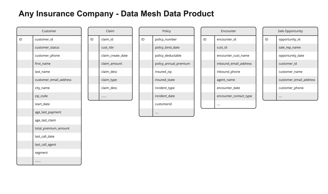
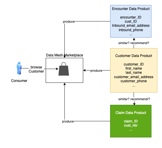

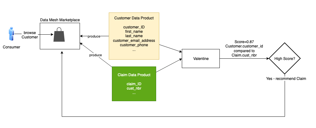
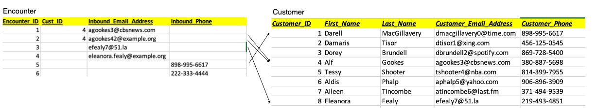
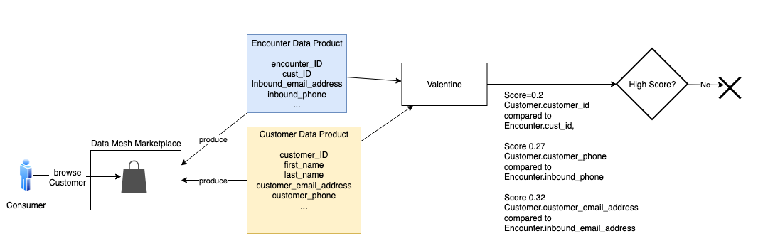
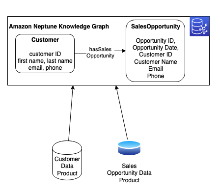
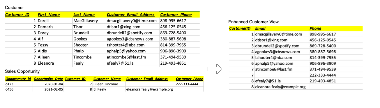
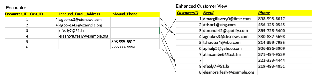
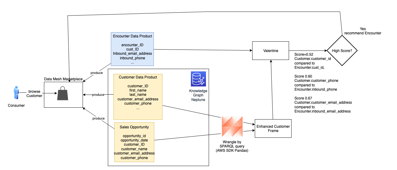
 Moira Lennox is a Senior Data Strategy Technical Specialist for AWS with 27 years’ experience helping companies innovate and modernize their data strategies to achieve new heights and allow for strategic decision-making. She has experience working in large enterprises and technology providers, in both business and technical roles across multiple industries, including health care live sciences, financial services, communications, digital entertainment, energy, and manufacturing.
 Joel Farvault is Principal Specialist SA Analytics for AWS with 25 years’ experience working on enterprise architecture, data strategy, and analytics, mainly in the financial services industry. Joel has led data transformation projects on fraud analytics, claims automation, and data governance.
 Mike Havey is a Solutions Architect for AWS with over 25 years of experience building enterprise applications. Mike is the author of two books and numerous articles. His
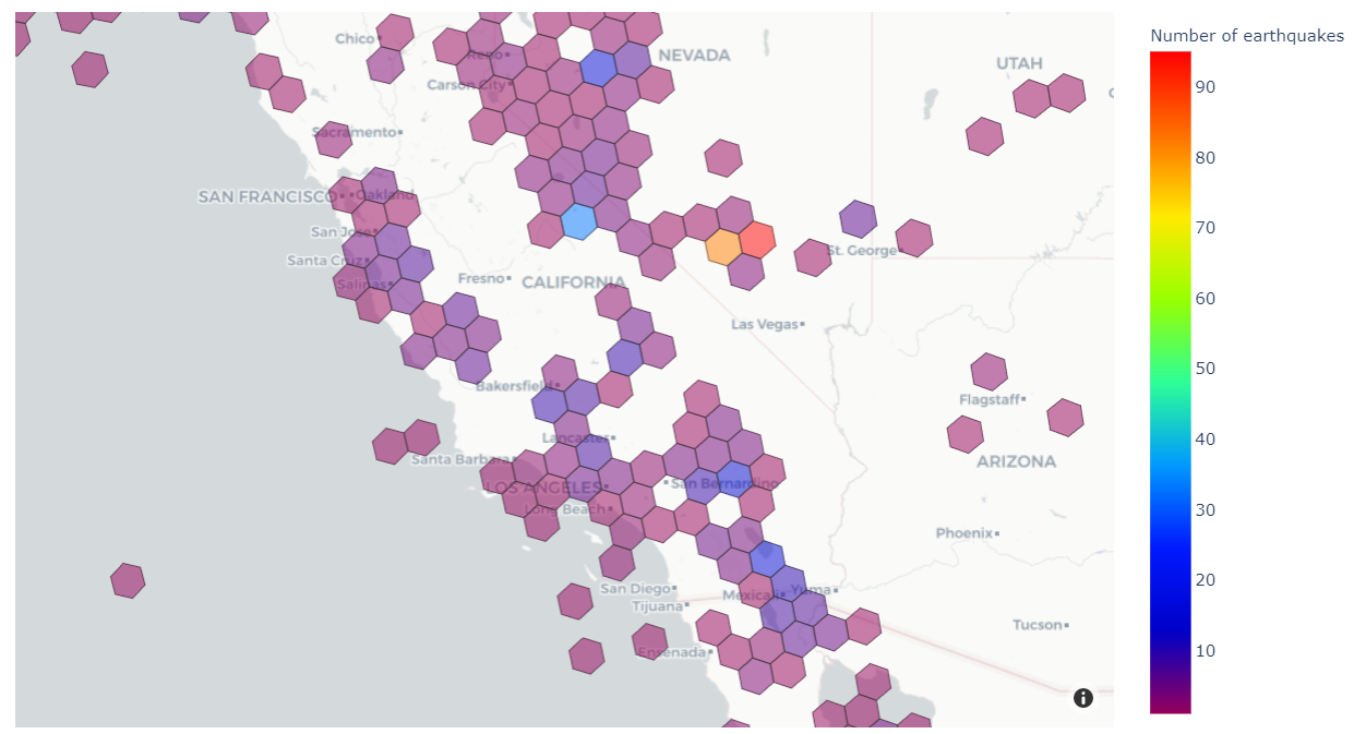


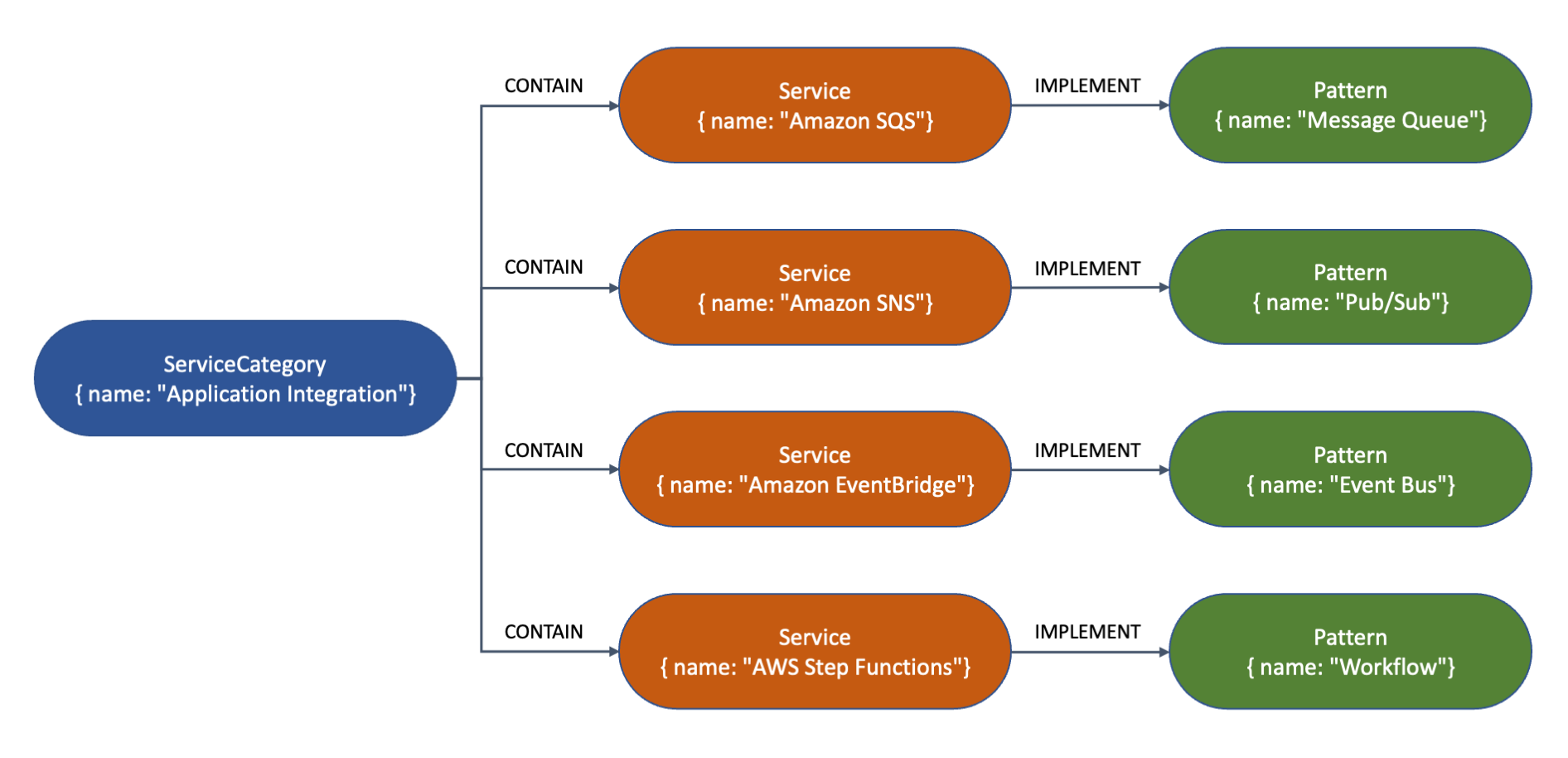
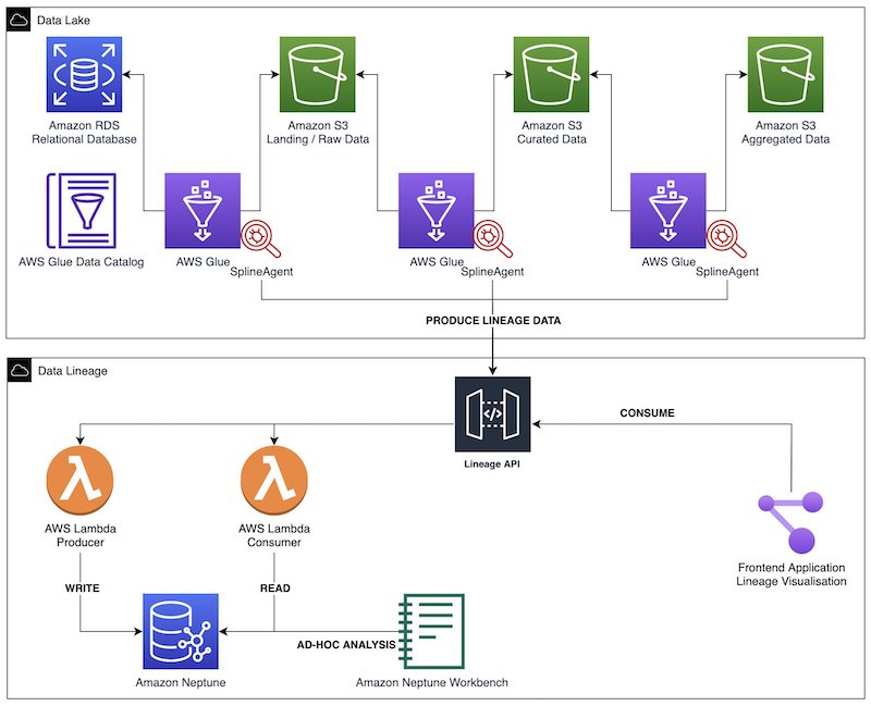
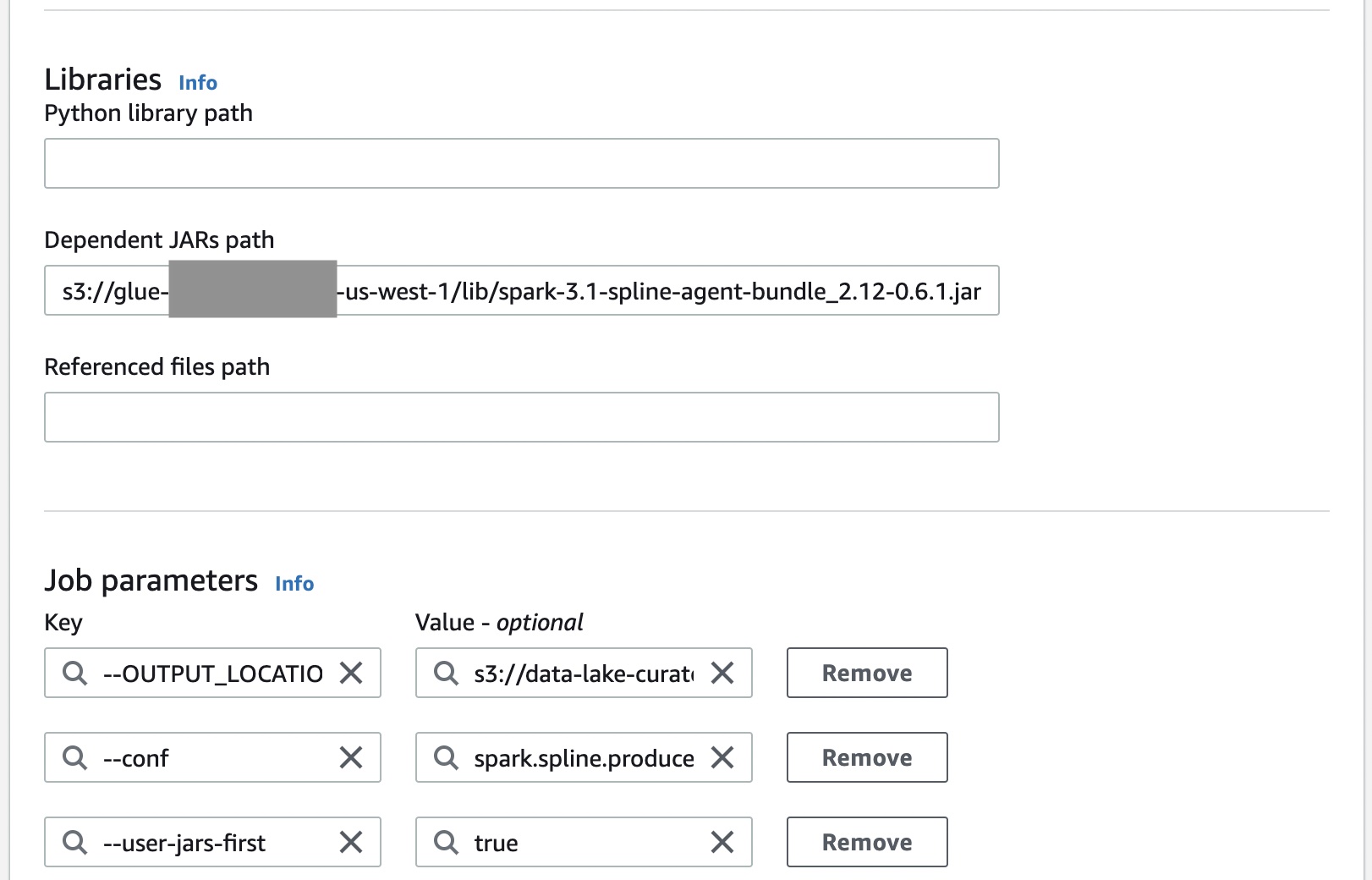
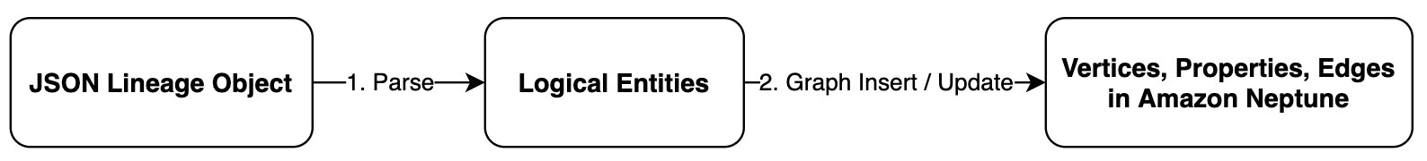

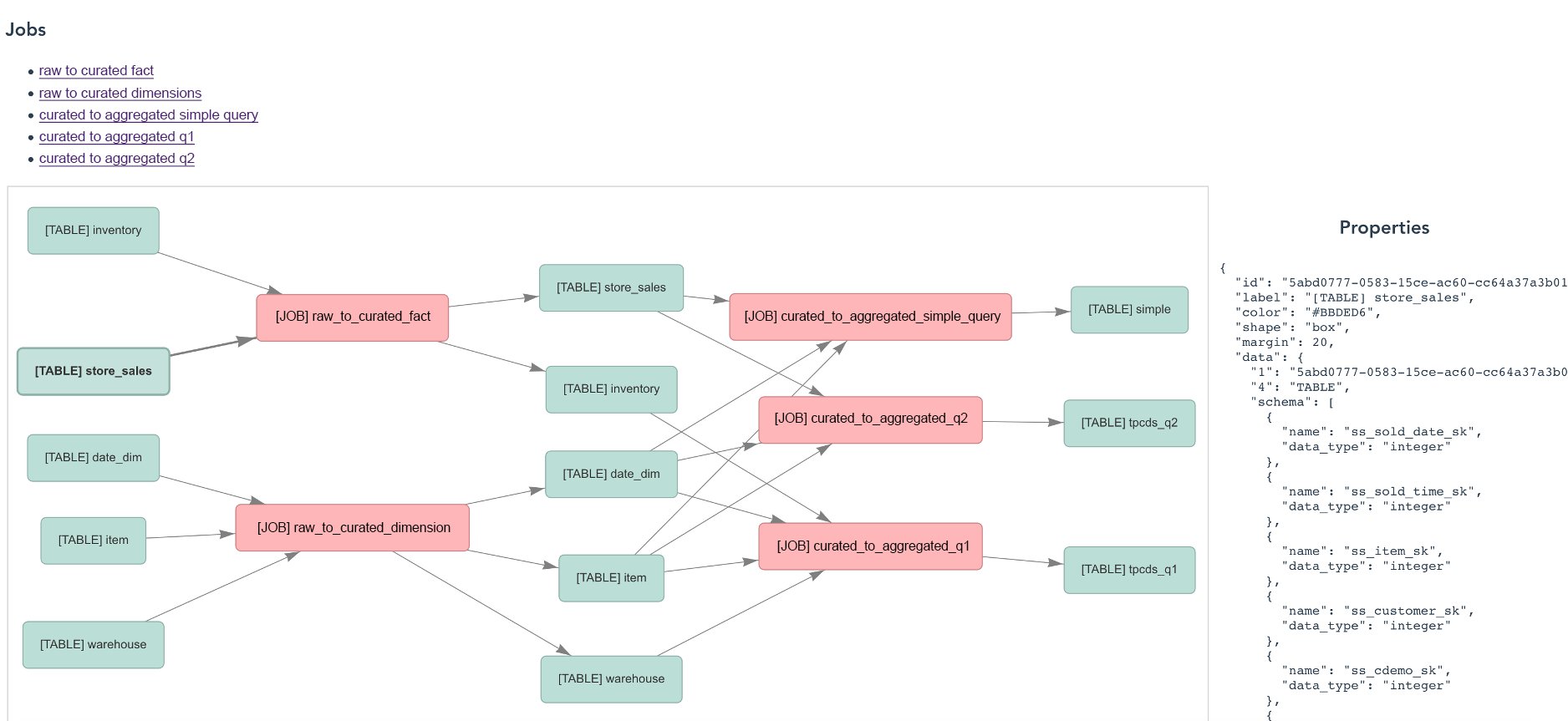

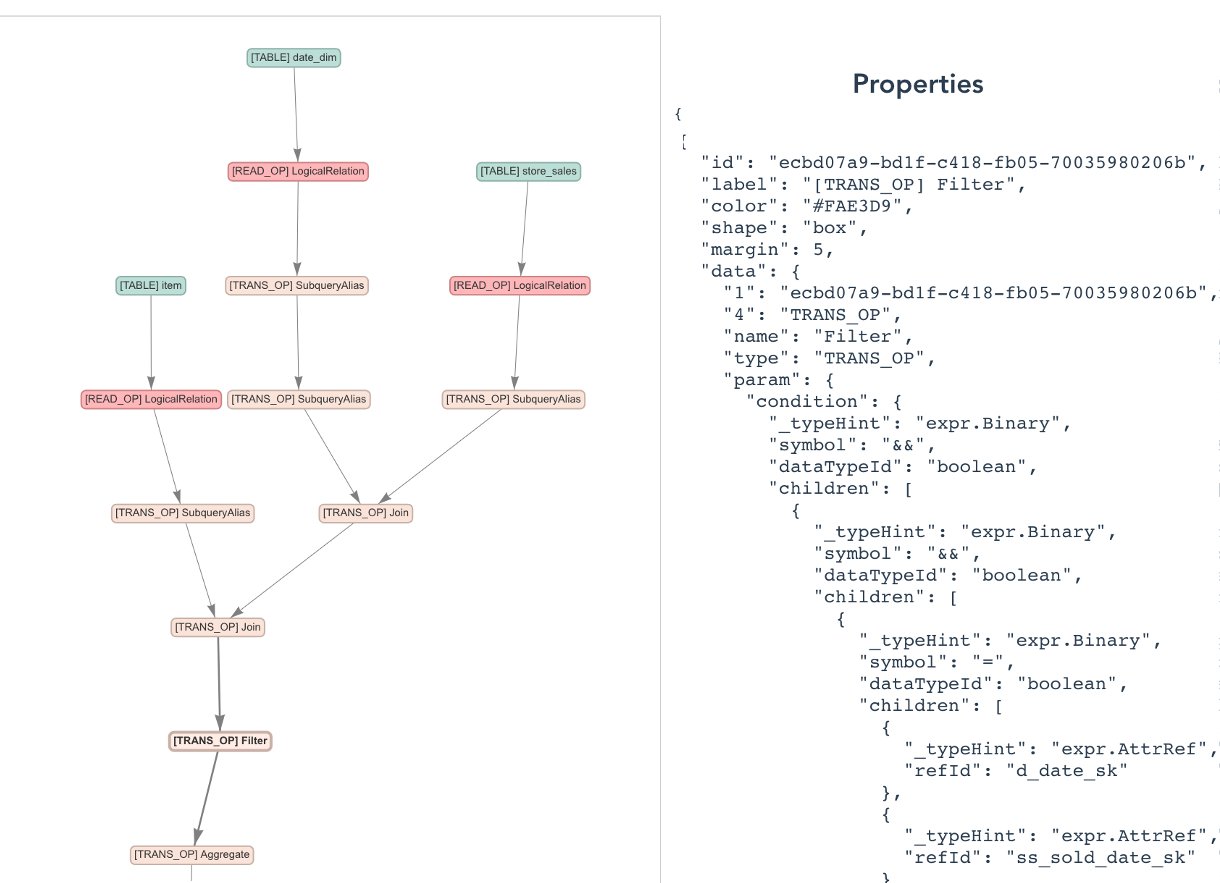


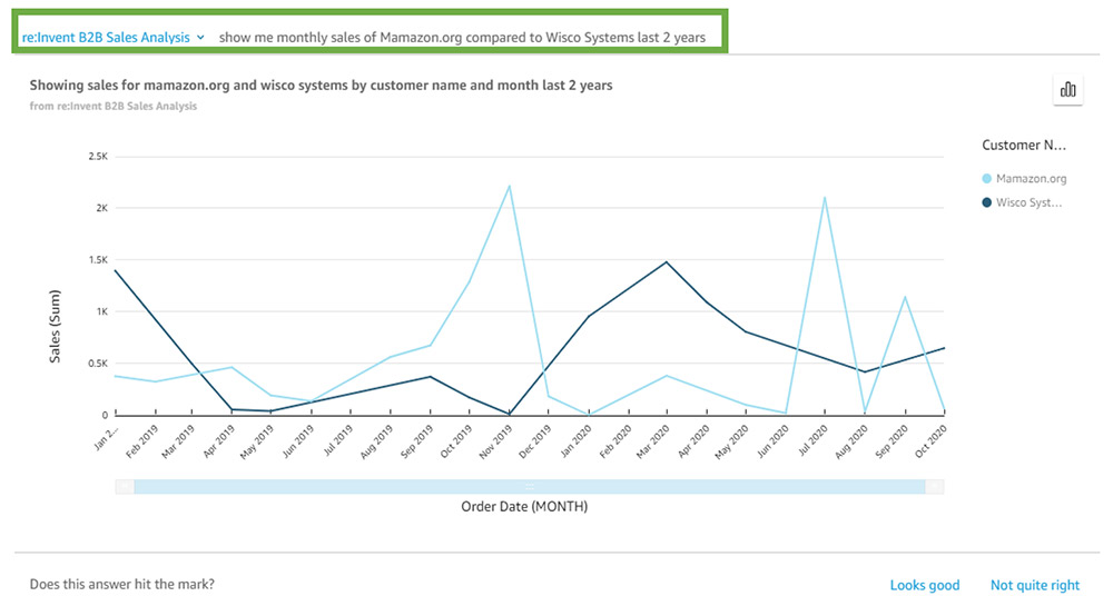

 Herain Oberoi leads Product Marketing for AWS’s Databases, Analytics, BI, and Blockchain services. His team is responsible for helping customers learn about, adopt, and successfully use AWS services. Prior to AWS, he held various product management and marketing leadership roles at Microsoft and a successful startup that was later acquired by BEA Systems. When he’s not working, he enjoys spending time with his family, gardening, and exercising.